Extraction of the CKM angle $\gamma$ from the new ”mixed ” system of $B^{+}\to\pi^{+}K^{0}$ and $B_{d}^{0}\to\pi^{0}K^{0}$ decays

Abstract

In this paper we try to extract the CKM angle $\gamma$ from the new ”mixed” system of $B^{+}\to\pi^{+}K^{0}$ and $B_{d}^{0}\to\pi^{0}K^{0}$ decays. We also made an update for the constraints on the angle $\gamma$ from the observables $R$ and $A_{0}$. In the parametrization, the $SU(2)$ isospin symmetry of strong interactions has been applied. We found the following results: (a) the measured value of $R$ is now very close to unit, the bound on the angle $\gamma$ from the measurement of $R$ is therefore not as promising as before, but some bounds on $\gamma$ can still be read off from $r-\gamma$ plane if $r$ could be fixed by using an additional input; (b) the measured $R_{1}$ implies a limit on the strong phase $\Delta_{1}$; (c) due to the contribution from the color allowed electroweak penguin, the minimal value of $R_{1}$ can be larger than unit. For $\epsilon_{1}=0.2$ and $R_{1}=1.2$, the range of $65^{\circ}\leq\gamma\leq 115^{\circ}$ will be excluded, such bounds on $\gamma$ are interesting and complimentary to the limits from global fit; (d) the dependences of extraction of $\gamma$ on the variation of parameters $\epsilon_{1}$, $\rho$, $r_{1}$ and strong phases are also studied.

PACS numbers: 13.25.Hw, 12.15.Hh, 12.15.Ji, 12.38.Bx

I Introduction

As is well known, one of the main goals of the B-factories is to measure the CKM angles $\alpha,\beta$ and $\gamma$[1, 2]. For the determination of the angle $\gamma$, $B\to\pi K,\pi\pi$ decay modes play a key role, and have been studied intensively in the literature [3, 4, 5, 6, 7]. Up to now, many two-body charmless B meson decays have been observed by CLEO, BaBar and Belle collaborations[8, 9, 10]. For the four $B\to K\pi$ decay modes considered here, the latest world average of the corresponding branching fractions are the following

$${\cal BR}(B\to\pi^{\pm}K^{\mp}) = (17.3\pm 1.5)\times 10^{-6},$$ (1)

$${\cal BR}(B^{\pm}\to\pi^{0}K^{\pm}) = (12.1\pm 1.7)\times 10^{-6},$$ (2)

$${\cal BR}(B^{\pm}\to\pi^{\pm}K^{0}) = (17.4\pm 2.6)\times 10^{-6},$$ (3)

$${\cal BR}(B\to\pi^{0}K^{0}) = (10.4\pm 1.7)\times 10^{-6},$$ (4)

The accuracy of the data is currently $10\%$ to $20\%$, and will be improved rapidly along with the progress of the experiments.

For the four $B\to K\pi$ decays, the isospin and $SU(3)$ flavor symmetries of strong interactions imply some important relations among their decay amplitudes [11]. Based on these amplitude relations, three combinations of CP-averaged $B\to\pi K$ branching ratios and the corresponding ”pseudo-asymmetries” have been considered [3, 4, 5, 6, 7] to probe the angle $\gamma$:

$$\left(\begin{array}[]{l}R\\ A_{0}\\ \end{array}\right) \equiv \frac{{\cal BR}(B_{d}^{0}\to\pi^{-}K^{+})\pm{\cal BR}(\overline{B_{d}^{0}}\to\pi^{+}K^{-})}{{\cal BR}(B^{+}\to\pi^{+}K^{0})+{\cal BR}(B^{-}\to\pi^{-}\overline{K^{0}})}$$ (7)

$$\left(\begin{array}[]{l}R_{c}\\ A_{0}^{c}\\ \end{array}\right) \equiv 2\frac{{\cal BR}(B^{+}\to\pi^{0}K^{+})\pm{\cal BR}(B^{-}\to\pi^{0}K^{-})}{{\cal BR}(B^{+}\to\pi^{+}K^{0})+{\cal BR}(B^{-}\to\pi^{-}\overline{K}^{0})},$$ (10)

$$\left(\begin{array}[]{l}R_{n}\\ A_{0}^{n}\\ \end{array}\right) \equiv \frac{1}{2}\frac{{\cal BR}(B_{d}^{0}\to\pi^{-}K^{+})\pm{\cal BR}(\overline{B_{d}^{0}}\to\pi^{+}K^{-})}{{\cal BR}(B_{d}^{0}\to\pi^{0}K^{0})+{\cal BR}(\overline{B_{d}^{0}}\to\pi^{0}\overline{K^{0}})},$$ (13)

where the factors of $2$ and $1/2$ have been introduced to absorb the $\sqrt{2}$ factors originating from the wavefunctions of $\pi^{0}$ meson. When CLEO firstly reported their observation of the decays $B_{d}\to\pi^{\pm}K^{\mp}$, $B^{\pm}\to\pi^{\pm}K$, the measured ratio $R=0.65\pm 0.40$ lead to an interesting bound on angle $\gamma$[3]. Since the measured $R$ is now very close to 1, however, the constraint on the angle $\gamma$ from this ”mixed” system is becoming weak now. For the possible constraints on $\gamma$ derived from the ”charged” and ”neutral” systems, one can see for example Refs.[6, 7] and references therein.

In this paper, we define and study a new ”mixed” system $B^{+}\to\pi^{+}K^{0}$ and $B_{d}^{0}\to\pi^{0}K^{0}$, to see if we can extract out or put some constraints on the angle $\gamma$ from the new observables, the ratio $R_{1}$ and the corresponding ”pseudo-asymmetry” $A_{1}$,

$$\left(\begin{array}[]{l}R_{1}\\ A_{1}\\ \end{array}\right) \equiv 2\frac{{\cal BR}(B_{d}^{0}\to\pi^{0}K^{0})\pm{\cal BR}(\overline{B}_{d}^{0}\to\pi^{0}\overline{K}^{0})}{{\cal BR}(B^{+}\to\pi^{+}K^{0})+{\cal BR}(B^{-}\to\pi^{-}\overline{K}^{0})}$$ (16)

We will also make an update for the constraint on the angle $\gamma$ from the observables $R$ and $A_{0}$.

Using the CP-averaged branching ratios as given in Eq.(4) one finds that

$$R = 0.99\pm 0.17,\ \ R_{1}=1.20\pm 0.36.$$ (17)

The central value of $R$ is very close to unit now.

This paper is organized as follows. In Sec.II, we present the general description of the $B\to\pi K$ decays, define the observables and make estimations about their magnitude. In Sec.III, we consider the new measured values of $R$ and $A_{0}$ to make an update for the bounds on $\gamma$ derived from the so-called ”mixed” system: $B^{+}\to\pi^{+}K^{0}$ and $B_{d}^{0}\to\pi^{+}K^{-}$ decay modes. In Sec.IV, we study the new ”mixed” system, $B^{+}\to\pi^{+}K^{0}$ and $B_{d}^{0}\to\pi^{0}K^{0}$ decays, to find the possible bounds on $\gamma$ from this new combination. The conclusions are included in the final section.

II General Description of $B\to\pi K$ decays

First of all, as illustrated in Fig.1, the Feynman diagrams contributing to the charmless $B\to\pi K$ decays can be classified as follows [11]:

• a color-favored ”tree” amplitude $T$ and a color-suppressed ”tree” amplitude $C$;

• a QCD penguin amplitude $P$;

• an color-allowed electroweak (EW) penguin amplitude $P_{EW}$, and a color-suppressed EW penguin amplitude $P^{C}_{EW}$;

• an annihilation amplitude ${\cal A}$.

The possible rescattering diagrams are not shown in Fig.1, one can see Fig.12 of Ref.[5] for some relevant rescattering diagrams.

Following Refs.[3, 11], the transition amplitudes for the four $B\to\pi K$ decays can be written as

$$A(B^{+}\to\pi^{+}K^{0}) = P+c_{d}P^{C}_{EW}+{\cal A}\;,$$ (18)

$$\sqrt{2}A(B^{+}\to\pi^{0}K^{+}) = -\left[P+T+C+P_{EW}+c_{u}P^{C}_{EW}+{\cal A}\right]\;,$$ (19)

$$A(B_{d}^{0}\to\pi^{-}K^{+}) = -\left[P+T+c_{u}P^{C}_{EW}\right]\;,$$ (20)

$$\sqrt{2}A(B_{d}^{0}\to\pi^{0}K^{0}) = \left[P-C\right]-\left[P_{EW}-c_{d}P^{C}_{EW}\right]\;$$ (21)

where $c_{u}=2/3$ and $c_{d}=-1/3$ are the up- and down-type quark charges, respectively. Because of the small ratio $|V_{us}V^{*}_{ub}|/|V_{ts}V^{*}_{tb}|\approx 0.02$, the four $B\to\pi K$ decays are dominated by the QCD penguin $P$. Because of the large top quark mass, we have also to care about the EW penguins. The overall EW penguin amplitude should be ${\cal O}(10\%)$ that of the gluonic penguin $P$, module group-theoretic factors[11]. The EW penguins contribute in the color-suppressed form to $B^{+}\to\pi^{+}K^{0}$ and $B_{d}^{0}\to\pi^{-}K^{+}$ decays and are hence expected to play a minor role, whereas they contribute to $B_{d}^{0}\to\pi^{0}K^{0}$ and $B^{+}\to\pi^{0}K^{+}$ decays in the color-allowed form and may compete with tree-diagram-like topologies. Approximately, the contribution from $P_{EW}^{C}$ should be smaller than its color-allowed counterpart $P_{EW}$ by a factor of $0.2$ and is at most a $5\%$ effect in $b\to s$ transition relative to the dominant QCD penguin contribution.

The relative sizes of the diagrams corresponding to the $\bar{b}\to\bar{u}u\bar{s}$ and $\bar{b}\to\bar{s}$ transitions at the quark level have been estimated[11]:

$$1 : |P|,$$ (22)

$${\cal O}(\lambda) : |T|,|P_{EW}|,$$ (23)

$${\cal O}(\lambda^{2}) : |C|,|P^{C}_{EW}|,$$ (24)

$${\cal O}(\lambda^{3}) : |A|,$$ (25)

where the parameter $\lambda=0.22$ is used as a measure of the approximate relative sizes of the various contributions. One can regard the above hierarchies as a simple estimation [11] since a modest enhancement or suppression due to hadronic matrix element for example can turn an effect of ${\cal O}(\lambda^{n})$ into an effect of ${\cal O}(\lambda^{n\pm 1})$.

In Refs.[5, 7], the decay amplitudes of $B\to\pi^{+}K^{0}$ and $\pi^{-}K^{+}$ have been parametrized as follows

$$A(B^{+}\to\pi^{+}K^{0}) \equiv {\cal P}=-\left(1-\frac{\lambda^{2}}{2}\right)\lambda^{2}A\left[1+\rho e^{i\theta}e^{i\gamma}\right]{\cal P}_{tc},$$ (26)

$$A(B_{d}^{0}\to\pi^{-}K^{+}) = -\left[{\cal P}+T+P_{EW}^{C}\right],$$ (27)

with

$${\cal P}_{tc} \equiv |{\cal P}_{tc}|e^{i\delta_{tc}}=\left(P_{t}-P_{c}\right)+\left(P_{EW}^{C(t)}-P_{EW}^{C(c)}\right),$$ (28)

$$\rho e^{i\theta} = \frac{\lambda^{2}R_{b}}{1-\lambda^{2}/2}\left[1-\left(\frac{{\cal P}_{uc}+{\cal A}}{{\cal P}_{tc}}\right)\right],$$ (29)

$$T \equiv |T|e^{i\delta_{T}}e^{i\gamma},$$ (30)

$$P_{EW}^{C} \equiv -|P_{EW}^{C}|e^{i\delta_{ew}},$$ (31)

where $P_{q}$ and $P_{EW}^{C(q)}$ ($q\in\{u,c,t\}$) denote contributions from QCD penguin and color-suppressed electroweak penguin topologies with internal q quarks, respectively. ${\cal P}_{uc}$ is similar to ${\cal P}_{tc}$ in Eq.(28), $\theta$, $\delta_{tc}$, $\delta_{T}$ and $\delta_{ew}$ are CP-conserving strong phases, and

$$A = 0.85\pm 0.04,\ \ \lambda=0.221\pm 0.002,\ \ R_{b}=0.38\pm 0.08$$ (32)

are the usual CKM factors[2].

The ratio $R$ and the corresponding ”pseudo-asymmetry” $A_{0}$ then take the form[5]

$$R = 1+r^{2}+\epsilon^{2}-2r\epsilon\cos{(\delta-\Delta)}\cos{\gamma}-\frac{2r}{\omega}\left[\cos{\delta}\cos{\gamma}+\rho\cos{(\delta-\theta)}\right]$$ (34)

$$+\frac{2\epsilon}{\omega}\left[\cos{\Delta}+\rho\cos{(\Delta-\theta)}\cos{\gamma}\right],$$

$$A_{0} = A_{+}+\frac{2r}{\omega}\sin{\delta}\sin{\gamma}+\frac{2\epsilon}{\omega}\rho\sin{(\Delta-\theta)}\sin{\gamma}+2r\epsilon\sin{(\delta-\Delta)}\sin{\gamma},$$ (35)

where $A_{+}$ measures the direct CP violation in the decay $B^{+}\to\pi^{+}K^{0}$

$$A_{+} \equiv \frac{BR({B}^{+}\to\pi^{+}K^{0})-BR({B}^{-}\to\pi^{-}0\overline{K^{0}})}{BR(B^{+}\to\pi^{+}K^{0})+BR(B^{-}\to\pi^{-}\overline{K^{0}})}$$ (36)

$$= -\frac{2\rho}{\omega^{2}}\sin\theta\sin\gamma$$ (37)

with

$$\omega=\sqrt{1+2\rho\cos{\theta}\cos{\gamma}+\rho^{2}}.$$ (38)

The parameters $r$ and $\epsilon$, as well as the CP-conserving strong phases $\delta$ and $\Delta$, have been defined as follows

$$r \equiv \frac{|T|}{\sqrt{<|{\cal P}|^{2}>}},\ \ \epsilon\equiv\frac{|P_{EW}^{C}|}{\sqrt{<|{\cal P}|^{2}>}},$$ (39)

$$\delta \equiv \delta_{T}-\delta_{tc},\ \ \Delta\equiv\delta_{ew}-\delta_{tc},$$ (40)

with

$$<|{\cal P}|^{2}>\equiv\frac{1}{2}\left(|{\cal P}|^{2}+|\overline{{\cal P}}|^{2}\right).$$ (41)

Here the $\overline{{\cal P}}$ is the CP-conjugate modes of ${\cal P}$ and obtained by performing the substitution $\gamma\to-\gamma$.

For the decay $B\to\pi^{0}K^{0}$, one parametrization presented in Ref.[7] is

$$\sqrt{2}A(B_{d}^{0}\to\pi^{0}K^{0}) \equiv P_{n}=-\left(1-\frac{\lambda^{2}}{2}\right)\lambda^{2}A\left[1+\rho_{n}e^{i\theta_{n}}e^{i\gamma}\right]{\cal P}_{tc}^{n},$$ (42)

where ${\cal P}_{tc}^{n}$ and $\rho_{n}e^{i\theta_{n}}$ take the form

$${\cal P}_{tc}^{n} \equiv |{\cal P}_{tc}^{n}|e^{i\delta_{tc}^{n}},$$ (43)

$$\rho_{n}e^{i\theta_{n}} = \frac{\lambda^{2}R_{b}}{1-\lambda^{2}}\left[1-\left(\frac{{\cal P}_{uc}-{\cal C}}{{\cal P}_{tc}^{n}}\right)\right]$$ (44)

By using the isospin symmetry of strong interactions for the $u$ and $d$ quarks and the decay amplitude relations as given in Eqs.(18,21), we here parametrize the $B\to\pi^{0}K^{0}$ decay in a new way

$$\sqrt{2}A(B_{d}^{0}\to\pi^{0}K^{0})\equiv P_{n}={\cal P}-C-P_{EW},$$ (45)

with

$$C\equiv|C|e^{i\delta_{c}}e^{i\gamma}\ \ \ P_{EW}\equiv-|P_{EW}|e^{i\delta^{\prime}_{ew}},$$ (46)

where the term $C$ denotes the contributions due to the color-suppressed ”tree” diagrams, the quantity $P_{EW}$ includes contributions from the color-allowed EW penguin topologies, and the $\delta_{c}$ and $\delta^{\prime}_{ew}$ denote CP-conserving strong phases.

If we define the observables

$$r_{1} \equiv \frac{|C|}{\sqrt{<|{\cal P}|^{2}>}},\ \ \ \ \epsilon_{1}\equiv\frac{|P_{EW}|}{\sqrt{<|{\cal P}|^{2}>}},$$ (47)

$$\delta_{1} \equiv \delta_{c}-\delta_{tc},\ \ \ \ \Delta_{1}\equiv\delta^{\prime}_{ew}-\delta_{tc}$$ (48)

we then find the expressions for $R_{1}$ and $A_{1}$

$$R_{1} = 1+r_{1}^{2}+\epsilon_{1}^{2}+\frac{2r_{1}}{\omega}\left[\cos{\delta_{1}}\cos{\gamma}+\rho\cos{(\delta_{1}-\theta)}\right]$$ (50)

$$-\frac{2\epsilon_{1}}{\omega}\left[\cos{\Delta_{1}}+\rho\cos{(\Delta_{1}-\theta)}\cos{\gamma}\right]-2r_{1}\epsilon_{1}\cos{(\delta_{1}-\Delta_{1})}\cos{\gamma}$$

$$A_{1} = A_{+}-\frac{2r_{1}}{\omega}\sin{\delta_{1}}\sin{\gamma}-\frac{2\epsilon_{1}}{\omega}\rho\sin{(\Delta_{1}-\theta)}\sin{\gamma}+2r_{1}\epsilon_{1}\sin{(\delta_{1}-\Delta_{1})}\sin{\gamma},$$ (51)

where the parameters $\rho$, $\theta$, $\omega$ and the CP asymmetry $A_{+}$ have been defined previously. In Eqs.(50,51), the electroweak penguin and rescattering effects are taken into account in a general way.

From the estimated hierarchy between the different diagrams as given in Eq.(25), we get to know that

$$r\approx\epsilon_{1}\approx 0.2,\ \ r_{1}\approx\epsilon\approx 0.04.$$ (52)

Evaluations based on the generalized factorization approach indicated that[3, 7]

$$r|_{fact}=0.16\pm 0.05,\ \ \epsilon|_{fact}=0.01-0.03.$$ (53)

By direct calculations in the generalized factorization approach we find numerically that

$$r=0.14-0.20,\ \ \epsilon=0.01-0.04,$$ (54)

and

$$r_{1}=0.001-0.04,\ \ \epsilon_{1}=0.07-0.15$$ (55)

in the case of neglected rescattering effects. Of course, above estimations may be affected severely by rescattering effects, which is unfortunately still unknown at present. A reliable theoretical evaluation of $\rho$ is indeed very difficult and requires insights into the dynamics of strong interactions. In Ref.[5], Fleischer studied the rescattering processes of the kind

$$B^{+} \to\{F_{c}^{(s)}\}\to\pi^{+}K^{0},$$ (56)

$$B^{+} \to\{F_{u}^{(s)}\}\to\pi^{+}K^{0},$$ (57)

where $F_{c}^{(s)}\in\{\overline{D^{0}}D_{s}^{+},\overline{D^{0}}D_{s}^{*+},\cdots\}$ and $F_{u}^{(s)}\in\{\pi^{0}K^{+},\pi^{0}K^{*+},\cdots\}$, and found that (a) $\rho\approx 0$ if rescattering processes of type (56) played the dominant role in $B^{+}\to\pi^{+}K^{0}$ decay; (b) $\rho={\cal O}(10\%)$ if (57) is dominant; and (c) $\rho={\cal O}(\lambda^{2}R_{b})\approx 0.04$ if both (56) and (57) were similarly important.

III Bounds on $\gamma$ from $R$ and $A_{0}$: an update

In Refs.[3, 5, 7], the strategies to extract the CKM angle $\gamma$ from the ratio $R$ have been studied. Because of the refinement of the measured $R$ and the first measurement of $A_{+}$, we here make an update for this approach.

Very recently, CLEO, BaBar and Belle collaboration reported their first measurement about the CP violating asymmetries of $B\to\pi^{+}K^{-},\pi^{+}K^{0}$ and $\pi^{0}K^{+}$ decays [9, 12], as listed in Table I. Although the measured CP-violating asymmetries of three $B\to\pi K$ decay modes have large uncertainty and therefore are still consistent with zero, we believe that they will be measured with a good accuracy within one or two years. From the measured $R$ and ${\cal A}_{CP}(B\pm\to\pi^{\pm}K^{\mp})$, we find that

$$A_{0}\equiv{\cal A}_{CP}({B^{\pm}\to\pi^{\pm}K^{\mp}})\cdot R=-0.12\pm 0.13.$$ (58)

A recent theoretical calculation based on PQCD approach predicted that ${\cal A}_{CP}(B_{d}^{0}\to\pi^{\pm}K^{\mp})\approx-0.19$ for $\gamma\sim 60^{\circ}$ [13], which is consistent with the experimental measurements. It is reasonable for us to assume that $|A_{0}|\lesssim 0.2$.

The ratio $R$ and the asymmetry $A_{0}$ as given in Eqs.(34,35) depend on seven parameters: $r$, $\epsilon$, $\gamma$, $\rho$ and CP-conserving strong phases $\theta$, $\delta$ and $\Delta$. Although parameters $r$ and $\epsilon$ can be fixed through theoretical arguments, the parameter $\rho$ is most possibly smaller than $0.15$, other four parameters still remain unknown.

In Fig.2 we show the dependence of $R$ on the angle $\gamma$ for $\rho=0.1$, $\epsilon=0.04$, $r=0.2$, while assuming $(\theta,\delta,\Delta)=0^{\circ}$ (curve 1), $90^{\circ}$ (curve 2) or $180^{\circ}$ (curve 3). The solid curve corresponds to the standard model prediction obtained by employing the generalized factorization approach and using the input parameters as specified in Ref.[14]. The band between two horizontal dots lines shows the experimental measurement: $R^{exp}=0.99\pm 0.17$. From this figure, one can see that

• The ratio $R$ in the generalized factorization approach has a similar dependence on $\gamma$ with the ratio $R$ as given in Eq.(34) in the case of $(\theta,\delta,\Delta)=0^{\circ}$.

• The ranges of $\gamma<45^{\circ}$ and $\gamma>120^{\circ}$ can be excluded for extreme values ($0^{\circ}$ or $180^{\circ}$) of three strong phases. But such constraint on $\gamma$ will disappear for $\theta=\delta=\Delta=90^{\circ}$. In other words, no bounds on $\gamma$ can be extracted directly from the $R-\gamma$ plane due to our ignorance of the strong phases.

As shown in Ref.[5], however, the observable $A_{0}$ allow us to eliminate the strong phase $\delta$ in the expression of $R$. By assuming both the parameter $r$ and the strong phase $\delta$ in the expression of $R$ as ”free” parameters, one found the minimal value of $R$ as follows [5]

$$R_{min}=\kappa\sin^{2}\gamma+\frac{1}{\kappa}\left(\frac{A_{0}}{2\sin\gamma}\right)^{2},$$ (59)

with

$$\kappa=\frac{1}{\omega}\left[1+2(\epsilon\omega)\cos\Delta+(\epsilon\omega)^{2}\right].$$ (60)

where $\omega$ has been given in Eq.(38). Now $R_{min}$ is independent of both $r$ and $\delta$, the effects of electroweak penguin and rescattering are included through the parameters $\epsilon$, $\rho$ and $\theta$ appeared in $\kappa$ and $\omega$. By comparing the plots of $R_{min}-\gamma$ with the measured $R$ as given in Eq.(17), one may draw the bounds on the CKM angle $\gamma$.

As a first approximation, we neglect the rescattering and electroweak penguin effects (i.e. setting $\rho=\epsilon=0$ ). The value of $R_{min}$ therefore depends on $A_{0}$ and $\gamma$ only. The $\gamma-$dependence of $R_{min}$ for $A_{0}=0,0.1,0.2,0.3$ and $0.4$ is shown in Fig.3, which is identical with the Fig.1 of Ref.[5]. From Fig.3 we get to know that if $R$ is found to be smaller than $1$, the values of $\gamma$ implying $R_{min}>R$ would be excluded. The current measured value of $R$ is unfortunately very close to unit, it is also unlikely to become smaller than $1$ when more B decay events are available. The bound on $\gamma$ from measurement of $R$ is therefore not as promising as three years ago.

For given $A_{0}$, the dependence of $r$ on the angle $\gamma$ is of the form [5]

$$r=\sqrt{\left(R+\cos^{2}\gamma\right)\pm 2\sqrt{\cos^{2}\gamma\left(R-\frac{A_{0}^{2}}{4\sin^{2}\gamma}\right)}}$$ (61)

in the case of $\rho=\epsilon=0$. Fig.4a show such dependence for $R=0.99$, and $A_{0}=0$ (solid curve), $0.1$ (dots curve), $0.2$ (short-dashed curve). Fig.4b shows the same dependence of $r$ on the angle $\gamma$ but for $R=0.65$ as being used in Ref.[5]. The contours as shown in Figs.(4a,4b) are rather different. For $R=0.65$, the value of $r$ can not be smaller than $0.2$. For $R=0.99$, $r\approx 0.15$ as indicated by theoretical calculations based on ”factorization” is natural. For given $R$ and $A_{0}$, the allowed ranges of $\gamma$ could be read off from the figures if the parameter $r$ can be fixed by using an additional input. For $|A_{0}|=0.2$, $R=0.99$ and $r=0.2$, for example, the regions

$$0^{\circ}\leq\gamma\leq 32^{\circ},\ \ 82^{\circ}\leq\gamma\leq 98^{\circ},\ \ and\ \ 150^{\circ}\leq\gamma\leq 180^{\circ}$$ (62)

should be excluded. The above constraints are consistent with the limit on $\gamma$ obtained from the global fit [15]: $43^{\circ}<\gamma<87^{\circ}$ at the 95% C.L.

For more details of $\rho$ and $\epsilon$ dependence of $R_{min}$, one can see the original papers[5, 7]. The new measurement of $R$ and $A_{0}$ do not affect previous discussions.

IV Bounds on $\gamma$ from $R_{1}$ and $A_{1}$

Analogous to the cases of $R$ and $A_{0}$[3, 5, 7], the observables $R_{1}$ and $A_{1}$ may also lead to interesting bounds on $\gamma$. By comparing the expressions of $R_{1}$ and $A_{1}$ with those of $R$ and $A_{0}$, we find three special features

• Between the observables $(R_{1},A_{1})$ and $(R,A_{0})$, there is a direct transformation relation: $r\to-r_{1}$ and $\epsilon\to-\epsilon_{1}$.

• The parameter $r_{1}$ which describes the contributions of ”color-suppressed” tree diagram is small in size: its ”factorized” value is $(r_{1})_{fact}=0.001-0.04$ and can be neglected.

• The parameter $\epsilon_{1}$ which describes the contributions of ”color-allowed” electroweak penguins, however, may be large in size as given in Eq.(55), and usually can not be neglected.

Like the ratio $R$ and the asymmetry $A_{0}$, $R_{1}$ and $A_{1}$ also depend on seven parameters: $r_{1}$, $\epsilon_{1}$, $\rho$, CKM angle $\gamma$ and the strong phases $\theta$, $\delta_{1}$ and $\Delta_{1}$ as defined in Eqs.(29,48). The parameters $r_{1}$ and $\epsilon_{1}$ can be fixed through theoretical arguments. If one can neglect or treat $\rho$ parameter and three strong phases properly, one may determine or put constraint on the angle $\gamma$ from the measured $R_{1}$.

In Fig.5 we show the general dependence of the ratio $R_{1}$ in Eq.(50) on the angle $\gamma$ for $\rho=0.1$, $r_{1}=0.04$, $\epsilon_{1}=0.1$, while assuming $(\theta,\delta_{1},\Delta_{1})=0^{\circ}$ (curve 1), $90^{\circ}$ (curve 2) or $180^{\circ}$ (curve 3). The solid curve corresponds to the standard model prediction of $R_{1}$ obtained by employing the generalized factorization approach and using the input parameters as specified in Ref.[14]. The band between two horizontal dots lines shows the data: $R_{1}^{exp}=1.20\pm 0.36$. Obviously no constraint on the angle $\gamma$ can be obtained by comparing the measured $R_{1}$ with the theory directly. It seems that the current data prefer large strong phases (curve 3).

In case of neglected rescattering and the color-suppressed tree diagrams, the expression of $R_{1}$ in Eq.(50) can be greatly reduced into the form

$$R_{1}=1+\epsilon_{1}^{2}-2\epsilon_{1}\cos\Delta_{1}.$$ (63)

Now it depends on two parameters only. If one can fix the value of $\epsilon_{1}$ from theoretical arguments, the measured $R_{1}$ will imply limits on the strong phase $\Delta_{1}$. In Fig.6 we show the dependence of $R_{1}$ on the strong phase $\Delta_{1}$ for various values of $\epsilon_{1}$. For given $\epsilon_{1}=0.2$, the lower limit on $\Delta_{1}$ can be read off directly from this figure

$$\Delta_{1}\geq 115^{\circ},$$ (64)

for $R_{1}=1.2$. In other words, the measured $R_{1}$ prefers $\Delta_{1}\geq 90^{\circ}$, i.e. $\cos\Delta_{1}<0$.

Following the same procedure of Ref.[5], one can eliminate the strong phase $\delta_{1}$ in Eq.(50) and find the minimal value of the ratio $R_{1}$. For this purpose, we rewrite Eq.(50) and Eq.(51) as

$$R_{1} = R_{0}+2r_{1}\left(\sl h\cos{\delta_{1}}+\sl k\sin{\delta_{1}}\right)+r_{1}^{2},$$ (65)

$$A = \left(B\sin{\delta}-C\cos{\delta}\right)r_{1},$$ (66)

where the quantities

$$R_{0} = 1-2\frac{\epsilon_{1}}{\omega}\left[\cos{\Delta}+\rho\cos{(\Delta_{1}-\theta)}\cos{\gamma}\right]+\epsilon_{1}^{2},$$ (67)

$$\sl h = \frac{1}{\omega}\left(\cos{\gamma}+\rho\cos{\theta}\right)-\epsilon_{1}\cos{\Delta_{1}}\cos{\gamma},$$ (68)

$$\sl k = \frac{\rho}{\omega}\sin{\theta}-\epsilon_{1}\sin{\Delta_{1}}\cos{\gamma},$$ (69)

$$A = \frac{A_{1}-A_{+}}{2\sin{\gamma}}+\frac{\epsilon_{1}\rho}{\omega}\sin{(\Delta_{1}-\theta)},$$ (70)

$$B = -\left(\frac{1}{\omega}-\epsilon_{1}\cos{\Delta_{1}}\right),$$ (71)

$$C = \epsilon_{1}\sin{\Delta_{1}},$$ (72)

are independent of $r_{1}$. From Eq.(66), we get

$$\sin{\delta_{1}} = \frac{AB\pm C\sqrt{(B^{2}+C^{2})r_{1}^{2}-A^{2}}}{(B^{2}+C^{2})r_{1}},$$ (73)

$$\cos{\delta_{1}} = \frac{-AC\pm B\sqrt{(B^{2}+C^{2})r_{1}^{2}-A^{2}}}{(B^{2}+C^{2})r_{1}},$$ (74)

and then eliminate the strong phase $\delta_{1}$ in Eq.(65):

$$R_{1}=R_{0}-AD\pm E\sqrt{(B^{2}+C^{2})r_{1}^{2}-A^{2}}+r_{1}^{2},$$ (75)

with

$$D=2\left(\frac{hC-kB}{B^{2}+C^{2}}\right),\ \ \ E=2\left(\frac{hB+kC}{B^{2}+C^{2}}\right)$$ (76)

Treating now $r_{1}$ in Eq.(75) as a free variable, we find the minimal value of $R_{1}$

$$(R_{1})_{min}=t\sin^{2}{\gamma}+\frac{1}{t}\left(\frac{A_{1}}{2\sin{\gamma}}\right)^{2}$$ (77)

with

$$t=\frac{1}{\omega^{2}}\left[1-2\epsilon_{1}\omega\cos{\Delta_{1}}+\epsilon_{1}^{2}\omega^{2}\right].$$ (78)

This is an exact formulae derived without any approximation. The effects of electroweak penguin and rescattering processes are included through the parameter $\epsilon_{1}$, $\rho$ and $\theta$, respectively.

For $B\to\pi^{+}K^{0}$ and $\pi^{+}K^{-}$ decays the EW penguin contributes in the ”color-suppressed” form only and therefore play a minor role. For $B\to\pi^{0}K^{0}$ decay, however, the ”color allowed” electroweak penguin is important and should be taken into account. This is the main difference between two sets of observables $(R,A_{0})$ and $(R_{1},A_{1})$. For $\rho=0$ and $\epsilon_{1}\neq 0$, the minimal value of $R_{1}$ will depend on the angle $\gamma$, the parameter $\epsilon_{1}$, the pseudo-asymmetry $A_{1}$ and the strong phase $\Delta_{1}$, as illustrated in Figs.(7,8,9).

Fig.7 shows the dependence of $(R_{1})_{min}$ on the angle $\gamma$ for $\rho=0$, $\epsilon_{1}=0.2$, $\Delta_{1}=180^{\circ}$ (maximal effect) and $|A_{1}|=0$, $0.2$ and $0.4$. From Fig.7, we find that

• Due to the contribution from the ”color allowed” electroweak penguin, the value of $(R_{1})_{min}$ can be larger than unit now:

  $$R_{1}\geq t\sin^{2}\gamma$$ (79)

  for $A_{1}=0$. Here the function $t$ is larger than unit if $\cos\Delta_{1}<0$. The values of $\gamma$ implying $(R_{1})_{min}>R_{1}$ would be excluded. Numerically, the ranges around $\gamma=90^{\circ}$, i.e.

  $$58^{\circ}\leq\gamma\leq 122^{\circ},$$ (80)

  $$65^{\circ}\leq\gamma\leq 115^{\circ},$$ (81)

  $$80^{\circ}\leq\gamma\leq 100^{\circ},$$ (82)

  would be excluded for $R_{1}=1,1.2$ and $1.4$, respectively. According to current experimental measurements, $R_{1}\approx 1.2$ is indeed natural, the corresponding bounds on the angle $\gamma$ are thus practical and interesting. Such bounds are also complimentary to the limits from global fit.

• Around $\gamma=90^{\circ}$, the bound on $\gamma$ is approximately independent of $A_{1}$. The excluded regions around $\gamma=0^{\circ}$ and $180^{\circ}$, however, depend on the values of $A_{1}$.

For the minimal value of $R_{1}$, the EW penguin contribution is included through $t=1-2\epsilon_{1}\cos\Delta_{1}+\epsilon_{1}^{2}$ in the case of $\rho=0$. Fig.8 shows the dependence of $(R_{1})_{min}$ on the angle $\gamma$ for $\rho=0$, $|A_{1}|=0.2$, $\Delta_{1}=180^{\circ}$, $\epsilon_{1}=0.05,0.10,0.15$ and $0.20$. It is easy to see that $(R_{1})_{min}$ has a moderate dependence on the value of $\epsilon_{1}$. Using $\epsilon_{1}=0.1$ and $R_{1}=1.20$, the range of $83^{\circ}\leq\gamma\leq 97^{\circ}$ could be excluded.

Fig.9 shows the dependence of $(R_{1})_{min}$ on the angle $\gamma$ for $\rho=0$, $|A_{1}|=0.2$, $\epsilon_{1}=0.2$, $\Delta_{1}=90^{\circ},120^{\circ}$, $150^{\circ}$ and $180^{\circ}$. Obviously, $(R_{1})_{min}$ and thus the bound on $\gamma$ has a strong dependence on phase $\Delta_{1}$. The bound given in Eq.(64) is the first limit on $\Delta_{1}$ from the measured $R_{1}$, but its uncertainty is also large. To get a reliable bound on $\gamma$ from this strategy, one has to determine the value of $\Delta_{1}$ with a reasonable accuracy.

Now we check the effects of the rescattering. For the minimal value of $R_{1}$, the rescattering effects are included through $\omega=\sqrt{1+2\rho\cos\theta\cos\gamma+\rho^{2}}$, and maximum for $\theta=0^{\circ}$ or $180^{\circ}$. In Fig.10 we show the dependence of $(R_{1})_{min}$ on the angle $\gamma$ for $\rho=0$, $0.1$, and $0.2$, while assuming $\epsilon_{1}=0.2$, $\Delta_{1}=180^{\circ}$, $|A_{1}|=0.2$, and $\theta=0^{\circ}$ or $180^{\circ}$. As shown in Fig.10, $(R_{1})_{min}$ has a weak dependence on $\rho$ only: its maximum around $\gamma=90^{\circ}$ is almost independent of $\rho$. The uncertainty of the bound on the angle $\gamma$ for a given $R_{1}$ is at most $10^{\circ}$ in the range of $\rho=0-0.2$.

According to the estimated hierarchy and direct calculation in generalized factorization approach, the parameter $r_{1}$ should be very small: $0\leq r_{1}\leq 0.04$. By treating the $\delta_{1}$ in Eq.(65) as a free parameter, on the other hand, one can also put the lower and upper bounds on $r_{1}$ from the measured $R_{1}$

$$(r_{1})_{min}^{max}=\left|\sqrt{R_{0}-t\sin^{2}\gamma}\pm\sqrt{R_{1}-t\sin^{2}\gamma}\right|.$$ (83)

where $R_{0}$ and $t$ have been given in Eqs.(67,78). Fig.11 shows the allowed regions of $r_{1}$ for $\rho=0$, $\epsilon_{1}=0.2$, $\Delta_{1}=180^{\circ}$ and for various values of $R_{1}$ corresponding to its currently allowed experimental range $R_{1}=1.20\pm 0.36$. From this figure, one can see that

• Small values of $R_{1}$ requires large values of $r_{1}$. For $R_{1}=0.84$, for example, the minimal value of $r_{1}$ is $0.28$, which is much larger than the theoretical estimations: $r_{1}\sim 0.04$. For $R_{1}\geq 1.2$, however, the minimal values of $r_{1}$ become compatible with the theoretical estimations.

• If $r_{1}$ could be fixed by using an additional input, the bounds on $\gamma$ can be read off directly from Fig.11. For $R_{1}=1.40$ and $r_{1}=0.05$, for example, the range of

  $$78^{\circ}\leq\gamma\leq 102^{\circ}$$ (84)

  could be excluded.

V Conclusions

In this paper we defined and studied a new ”mixed” system, $B^{+}\to\pi^{+}K^{0}$ and $B_{d}^{0}\to\pi^{0}K^{0}$ decays, to extract or constrain the CKM angle $\gamma$ from the measured ratio $R_{1}$ and the corresponding ”pseudo-asymmetry” $A_{1}$. We also made an update for the constraints on the angle $\gamma$ from the observables $R$ and $A_{0}$.

In the parameterization, the $SU(2)$ isospin symmetry of strong interactions for $u$ and $d$ quarks, the unitarity of the CKM matrix and the Wolfenstein parametrization of the CKM matrix have been applied. From the theoretical calculations and currently available experimental measurements, we found the following results:

• The measured value of $R$ is now very close to unit, the bound on the angle $\gamma$ from measurement of $R$ is therefore not as promising as three years ago. If $A_{0}$ is measured with good accuracy and $r$ can be fixed by theoretical arguments, however, some bounds on $\gamma$ are still possible. For $\rho=\epsilon=0$, $R=0.99$, $|A_{0}|=0.2$ and $r=0.2$, for example, the allowed regions of angle $\gamma$ can be read off from Fig.4

  $$30^{\circ}\leq\gamma\leq 82^{\circ},\ \ and\ \ 98^{\circ}\leq\gamma\leq 150^{\circ}.$$ (85)

• For $B_{d}^{0}\to\pi^{0}K^{0}$ decay, the color-allowed EW penguin play an important role. By direct calculations in the generalized factorization approach we find that

  $$r_{1}=0.001-0.04,\ \ \epsilon_{1}=0.07-0.15$$ (86)

  in the case of neglected rescattering effects, which agrees well with the estimated hierarchy of different Feynman diagrams.

• As shown in Fig.6, the measured $R_{1}$ implies a limit on the strong phase $\Delta_{1}$ in case of neglected rescattering and the color-suppressed tree diagrams. For given $\epsilon_{1}=0.2$ and $R_{1}=1.2$, the lower limit on $\Delta_{1}$ is $\Delta_{1}\geq 115^{\circ}$. This is the first limit on $\Delta_{1}$ from the measured $R_{1}$, but its uncertainty is still large.

• Due to the contribution from the ”color allowed” electroweak penguin, the minimal value of $R_{1}$ can be larger than unit, as illustrated in Fig.7. Using $\epsilon_{1}=0.2$ and $R_{1}=1.20$, the range of $65^{\circ}\leq\gamma\leq 115^{\circ}$ could be excluded, which is also approximately independent of $A_{1}$. These bounds on the angle $\gamma$ are interesting and complimentary to the limits from global fit.

• The bound on $\gamma$ has a moderate dependence on the value of $\epsilon_{1}$. Using $R_{1}=1.20$ and $\epsilon_{1}=0.1$, the range of $83^{\circ}\leq\gamma\leq 97^{\circ}$ could be excluded.

• The bound on $\gamma$ has a strong dependence on the strong phase $\Delta_{1}$. For $\Delta_{1}<90^{\circ}$, for example, the bound may disappear. To get a reliable bound on $\gamma$ from this strategy, one has to determine the value of $\Delta_{1}$ with a reasonable accuracy.

• The bound on $\gamma$ has a weak dependence on the rescattering effects only. The uncertainty of the bound on the angle $\gamma$ for a given $R_{1}$ is at most $10^{\circ}$ in the range of $\rho=0-0.2$.

• The bounds on $\gamma$ can be read off directly from $r_{1}-\gamma$ plane if $r_{1}$ could be fixed by using an additional input.

TABLE I.: Measurements of CP-violating asymmetry as reported by CLEO, BaBar and Belle Collaborations. The numbers in second entries are the ${\cal A}_{CP}$ at $90\%$ C.L. The last column lists the average.

Channel	CLEO	BaBar	Belle	Average
${\cal A}_{CP}(B^{\pm}\to\pi^{0}K^{\pm})$	$-0.29\pm 0.23$	$0.00\pm 0.18\pm 0.04$	$-0.06^{+0.22}_{-0.20}$	$-0.10\pm 0.12$
	$[-0.67,0.09]$	$[-0.30,0.30]$	$[-0.40,0.36]$
${\cal A}_{CP}(B\to\pi^{\mp}K^{\pm})$	$-0.04\pm 0.16$	$-0.19\pm 0.10\pm 0.03$	$0.04^{+0.19}_{-0.17}$	$-0.12\pm 0.08$
	$[-0.30,0.22]$	$[-0.35,-0.03]$	$[-0.25,0.37]$
${\cal A}_{CP}(B^{\pm}\to\pi^{\pm}K^{0})$	$+0.18\pm 0.24$	$-0.21\pm 0.18\pm 0.03$	$0.10^{+0.43}_{-0.34}$	$-0.05\pm 0.14$
	$[-0.22,0.56]$	$[-0.51,0.09]$	$[-0.53,0.82]$

FIG. 1.: Feynman diagrams contributing to $B\to K\pi$ decays. The $q$ denotes the $u$ or $d$ quarks.

FIG. 2.: The dependence of $R$ on $\gamma$ for $\rho=0.1$, $\epsilon=0.04$, $r=0.2$, while assuming $(\theta,\delta,\Delta)=0^{\circ}$ (curve 1 ), $90^{\circ}$ (curve 2) and $180^{\circ}$ (curve 3 ). The solid curve is the standard model prediction based on the generalized factorization approach. The band between two dots lines corresponds to the data: $R=0.99\pm 0.17$.

FIG. 3.: The dependence of $R_{min}$ on $\gamma$ for $|A_{0}|=0,0.1,0.2,0.3$ and $0.4$ in case of neglected EW penguin and rescattering effects.

FIG. 4.: The dependence of $r$ on the angle $\gamma$ for $R=0.99$ (a) and $0.65$ (b), and for $|A_{0}|=0$ (solid curve), $0.1$ (dots curve) and $0.2$ (short-dashed curve) in the case of $\rho=\epsilon=0$.

FIG. 5.: The dependence of $R_{1}$ on $\gamma$ for $\rho=0.1$, $r_{1}=0.04$, $\epsilon_{1}=0.1$, while assuming $(\theta,\delta,\Delta)=0^{\circ}$ (curve 1 ), $90^{\circ}$ (curve 2) and $180^{\circ}$ (curve 3 ). The solid curve is the standard model prediction of $R_{1}$ by employing the generalized factorization approach. The band between two dots lines corresponds to the data: $R_{1}=1.20\pm 0.36$.

FIG. 6.: The dependence of $R_{1}$ on the strong phase $\Delta_{1}$ for $\rho=r_{1}=0$, and $\epsilon_{1}=0.05,0.10,0.15$ and $0.2$.

FIG. 7.: The dependence of the minimal value of $R_{1}$ on the angle $\gamma$ for $\rho=0$, $\epsilon_{1}=0.2$, $\Delta_{1}=180^{\circ}$ and $|A_{1}|=0,0.2$ and $0.4$.

FIG. 8.: The dependence of the minimal value of $R_{1}$ on the angle $\gamma$ for $\rho=0$, $A_{1}=0.2$, $\Delta_{1}=180^{\circ}$, $\epsilon_{1}=0.05$, $0.10$, $0.15$ and $0.2$.

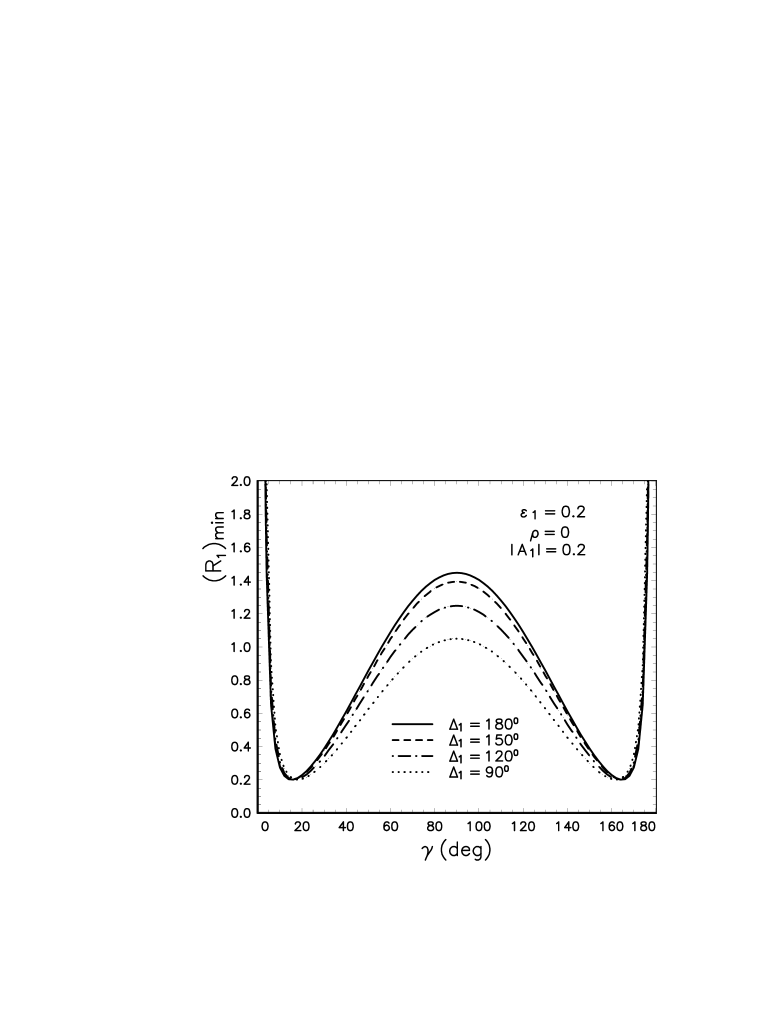
FIG. 9.: The dependence of the minimal value of $R_{1}$ on the angle $\gamma$ for $\rho=0$, $\epsilon_{1}=0.2$, $|A_{1}|=0.1$, $\Delta_{1}=0^{\circ}$, $45^{\circ}$, $90^{\circ}$, $135^{\circ}$ and $180^{\circ}$.

FIG. 10.: The rescattering effects on $(R_{1})_{min}$ for $\rho=0,0.10$ and $0.15$, while assuming $\epsilon_{1}=0.1$, $\Delta_{1}=180^{\circ}$, $|A_{1}|=0.2$, $\theta\in\{0^{\circ},180^{\circ}\}$. The curves for a given value of $\rho$ correspond to $\theta\in\{0^{\circ},180^{\circ}\}$ and show the maximum shift from $\rho=0$.

FIG. 11.: The allowed regions of the parameter $r_{1}$ for $\rho=0$, $\epsilon_{1}=0.2$, $\Delta=180^{\circ}$, and $R_{1}^{exp}=0.84,1.20,1.40$ and $1.56$.