The Proton Spin Problem
in the Chiral Bag Model

Hee-Jung Lee

Supervised by
Professor Dong-Pil Min

A Dissertation
Submitted to the Faculty of
Seoul National University
in Partial Fulfillment of
the Requirements for the Degree of
Doctor of Philosophy
Febrary 2002

Department of Physics
Graduate School
Seoul National University

Abstract

The flavor singlet axial charge has been a source of study in the last years due to its relation to the so called Proton Spin Problem. The relevant flavor singlet axial current is anomalous, i.e., its divergence contains a piece which is the celebrated $U_{A}(1)$ anomaly. This anomaly is intimately associated with the $\eta^{\prime}$ meson, which gets its mass from it. When the gauge degrees of freedom of QCD are confined within a volume as is presently understood, the $U_{A}(1)$ anomaly is known to induce color anomaly leading to “leakage” of the color out of the confined volume (or bag). For consistency of the theory, this anomaly should be cancelled by a boundary term. This “color boundary term” inherits part or most of the dynamics of the volume (i.e., QCD). In this thesis, we exploit this mapping of the volume to the surface via the color boundary condition to perform a complete analysis of the flavor singlet axial charge in the chiral bag model using the Cheshire Cat Principle. This enables us to obtain the hitherto missing piece in the axial charge associated with the gluon Casimir effect. The result is that the flavor singlet axial charge is small independent of the confinement (bag) size ranging from the skyrmion picture to the MIT bag picture, thereby confirming the (albeit approximate) Cheshire Cat phenomenon.


Key words : Flavor singlet axial charge, proton, spin, $U_{A}(1)$ anomaly, $\eta^{\prime}$ meson, gluon, Casimir effect
Student number : 95303-823

Chapter 1 Introduction

The constituent quark was proposed to explain the structure of the large number of hadrons being discovered in the sixties [2]. Soon thereafter deep inelastic scattering of leptons off protons was explained in terms of point-like constituents named partons [3]. The analysis of the data by means of sum rules led to the conclusion that there was an intimate relation between the partons and the elementary quarks. Various models have been developed to understand the structures of light hadrons and their interactions in terms of quarks [4]. They were built on the basis of low-energy hadron phenomenologies, particularly, (i) approximate $SU(3)$ flavor symmetry and its explicit breaking, (ii) Okubo-Zweig-Izuka (OZI) suppression rule for flavor changing processes [5], and (iii) chiral symmetry realization with its spontaneous breaking pattern.

The birth of Quantum Chromodynamics (QCD) and the proof that it is asymptotically free set the framework for an understanding of deep inelastic phenomena beyond the parton model [6]. However the fact that QCD confines does not allow a solution of the theory in the strong coupling regime and therefore new models had to be developed to describe hadron structure which realized the phenomenological principles mentioned before but in a manner compatible with the dynamical principles of the theory. This scheme of confined isolated quarks and gluons, has a strong relation to the valence quark model for hadrons [7]. The valence quark model was developed further to a non-relativistic quark model by De Rújula, Georgi and Glashow [8] initially and exploited phenomenologically by Isgur and Karl [9], and into a relativistic quark model framework by Chodos et al. and De Grand et al. known under the name of MIT bag model [10].

Although the MIT bag model was successful in describing the properties of the nucleons, it was not pertinent due to lack of the chiral symmetry. In order to incorporate chiral symmetry into the model, the pseudoscalar mesons had to be introduced in this framework [11]. The resulting scheme, the so called chiral bag model, was constructed with meson fields which are restricted to be outside the bag [12].

Chiral symmetry, a property of QCD with massless quarks, has been instrumental in the description of hadron phenomenology. So much so, that Skyrme realized its importance and wrote down, much before QCD, an effective theory for the strong interactions, in terms of pion fields only, describing a unified theory for baryons and mesons [13]. Only many years later his tremendous intuition was appreciated and his ideas justified from the point of view of QCD [14].

The chiral bag model incorporates in a unified description the statements above. It is defined by means of a QCD lagrangian inside the bag and by a Skyrme type theory outside, properly matched at the surface to preserve the classical and quantum symmetries. These formulation leads to a intriguing principle referred to as the Chesire Cat Principle (CCP) [15, 16]. The possibility of formulating a physical theory by means of equivalent field theories defined in terms of different field variables, leads to this construction principle for phenomenologically sensible and conceptually powerful models. This principle states, that physical observables obtained by means of equivalent theories defined in a certain space-time geometry, adequately matched at the boundaries, are independent of the geometry. In 1+1 dimensions fermionic theories are bosonizable [17] and the CCP can be made exact and transparent. In the real four-dimensional world, bosonization with a finite number of degrees of freedom is not exact. However based on the unproven “theorem” of Weinberg [18], it seems possible to argue that the CCP should hold also in four dimensions, albeit approximately.

Quantum Chromodynamics (QCD) is the theory of the hadronic phenomena [6]. At sufficiently low energies or long distances and for a large number of colors $N_{C}$, it can be described accurately by an effective field theory in terms of meson fields [14, 19]. In this regime, the color fermionic description of the theory is extremely complex due to confinement. However the implementation of the CCP in a two phase scenario called the Chiral Bag Model (CBM) has proven surprisingly powerful [20]. The CBM is defined by dividing space-time in two regions by a hypertube, that is, the evolving bag. In the interior of the tube, the dynamics is defined in terms of the microscopic QCD degrees of freedom, quarks and gluons. In the exterior, one assumes an equivalent dynamics in terms of meson fields, i.e., one that respects the symmetries of the original theory and the basic postulates of quantum field theory [18]. The two descriptions are matched by defining the appropriate boundary conditions which implement the symmetries and confinement [15, 20]. What this does effectively is to delegate all or part of the principal elements of the dynamics taking place inside (QCD) the bag to the boundary. We will see that this strategy works quite efficiently in the problem at hand. In this scenario the CCP states that the hadron physics should be approximately independent of the spatial size of the confinement region or the bag [15]. This realization of the principle has been tested in many instances in hadronic physics with fair success [16].

There is one case, however, where the realization of the CCP has not been as successful as in the other cases, namely, the calculation of the flavor singlet axial charge (FSAC) of the nucleon. Indeed in the previous results [21, 22, 23], the CCP was realized only partially as it seemed to fail at certain points such as for zero bag radius. It is the leitmotiv of this work to remove this apparent failure.

Experiments using polarized electrons on polarized targets were carried out at SLAC [24]. Further information came from the SLAC-Yale group with fascinating implications about the internal structure of the proton [25]. More recently, the European Muon Collaboration (EMC) obtained very extraordinary results by the scattering of a polarized muon beam with energy 100-200 GeV on a longitudinally polarized hydrogen target at CERN [26]. All these results point towards a new scenario in hadronic structure dominated by a quantum anomaly. To be more specific, the unexpectedly small asymmetry found by EMC implies a strong violation of the so-called Ellis-Jaffe sum rule [27] and therefore implies that the polarization of the proton is not carried exclusively by the valence quarks. This problem is called the Proton Spin Problem [28].

The EMC result and this problem are now believed to be resolved through the beautiful relation between the flavor singlet axial charge and the axial anomaly [29] [30]:

$$a^{0}(Q^{2})=\Delta\Sigma-N_{F}\frac{\alpha_{s}(Q^{2})}{2\pi}\Delta g(Q^{2}),$$ (1.1)

where $a^{0}(Q^{2})$ is the flavor singlet axial charge measured by EMC, $\Delta\Sigma$ the quark polarization, and $\Delta g(Q^{2})$ the gluon polarization.

The aim of this thesis is to show the full consistency of the CCP in the hadronic world for the case of the Proton Spin, which was not satisfactorily established in the previous results in this direction [21, 22, 23]111Note that in these papers, they have shown that the CCP holds for non-zero bag radii but it failed when the bag radius shrank to a point, implying that in the model studied, the pure skyrmion and the MIT bag did not have the equivalent structure required by the CCP..

In the CBM, the scenario of how the CCP is realized – which is the central issue of this thesis – is very intricate. As stated, the flavor singlet axial current is associated with the anomaly and effectively with the $\eta^{\prime}$ meson. Thus, besides the pion field of the conventional effective theories which accounts for spontaneously broken chiral symmetry, the correct treatment of the flavor singlet axial charge requires minimally the inclusion of a field describing the $\eta^{\prime}$ meson.

The intricacies of the hedgehog configuration and its relevance to the fractionation of baryon charge and other observables have been extensively discussed [31] and fairly well understood [32, 33]. They will be implemented in the present calculation without much details. Moreover the inclusion of the $\eta^{\prime}$ meson carries subtleties of its own. The vacuum fluctuations inside the bag, that induce the baryon number leakage into the skyrmion [31], also induce a color leakage if a coupling to a pseudoscalar isoscalar field is allowed [34]. This leakage would break color gauge invariance and confinement in the model unless it is cancelled. As suggested in [34], this color leakage can be prevented by introducing into the CBM Lagrangian a counter term of the form

$${\cal L}_{CT}=i\frac{g_{s}^{2}}{32\pi^{2}}\oint_{\Sigma}d\beta\ K^{\mu}n_{\mu}({{\rm Tr}}{{\rm ln}}U^{\dagger}-{{\rm Tr}}{{\rm ln}}U)$$ (1.2)

where $N_{F}$ is the number of flavors (here taken to be =3), $\beta$ is a point on a surface $\Sigma$, $n^{\mu}$ is the outward normal to the bag surface, $U$ is the $U(N_{F})$ matrix-valued field written as $U=e^{i\pi/f}e^{i\eta^{\prime}/f_{0}}$ and $K^{\mu}$ the properly regularized Chern-Simons current $K^{\mu}=\epsilon^{\mu\nu\alpha\beta}(G_{\nu}^{a}G_{\alpha\beta}^{a}-\frac{2}{3}g_{s}f^{abc}G_{\nu}^{a}G_{\alpha}^{b}G_{\beta}^{c})$ given in terms of the color gauge field $G^{a}_{\mu}$. Note that the counter term (1.2) manifestly breaks color gauge invariance (both large and small, the latter due to the bag), so the action of the chiral bag model with this term is not gauge invariant at the classical level but as shown in [34], when quantum fluctuations are calculated, there appears an induced anomaly term on the surface which exactly cancels this term. Thus gauge invariance is restored at the quantum level.

The equations of motion for the gluon and quark fields inside and the $\eta^{\prime}$ field outside are the same as in [21, 22]. However the boundary conditions on the surface with the inclusion of eq. (1.2) read [23]

$$\hat{\bf n}\cdot{\bf E}^{a}=-\frac{N_{F}g_{s}^{2}}{8\pi^{2}f}\hat{\bf n}\cdot{\bf B}^{a}\eta^{\prime}$$ (1.3)
$$\hat{\bf n}\times{\bf B}^{a}=\frac{N_{F}g_{s}^{2}}{8\pi^{2}f}\hat{\bf n}\times{\bf E}^{a}\eta^{\prime}$$ (1.4)

and

$$\frac{1}{2}\hat{\bf n}\cdot({\bar{\psi}}\mbox{\boldmath$\gamma$}\gamma_{5}\psi)=f\hat{\bf n}\cdot\partial\eta^{\prime}+\frac{N_{F}g_{s}^{2}}{16\pi^{2}}\hat{\bf n}\cdot K$$ (1.5)

where ${\bf E}^{a}$ and ${\bf B}^{a}$ are, respectively, the color electric and color magnetic fields. Here $\psi$ is the QCD quark field.

The full Casimir calculation of the gluon modes, which is highly subtle due to the p-wave structure of the $\eta^{\prime}$-field, has to be performed to get the CCP for the flavor singlet axial charge. Here we would like to side-step this technically difficult procedure by first assuming the CCP in evaluating the Casimir contribution with the color boundary conditions (1.3), (1.4) and (1.5) taken into account and check a posteriori that there is consistency between the assumption and the result.

The thesis is organized as follows: In Chapter 2, we introduce the Proton Spin Problem via the polarized deep inelastic scattering experiments and the relation between the spin dependent structure function, $g_{1}(x)$, and the flavor singlet axial charge. A general review of the chiral bag model is given in Chapter 3 for the next discussion. In Chapter 4, we review the axial anomaly and present its contribution to the flavor singlet axial charge. Moreover, we show a derivation of the color anomaly boundary condition. We address the various static contributions and calculate the Casimir effect to the flavor singlet axial charge in Chapter 5. Finally, we discuss our result in Chapter 6.

Chapter 2 Proton Spin Problem

Deep inelastic lepton-hadron scattering (DIS) has played an important role in understanding the internal structure of hadrons. The discovery of Bjorken scaling in the late nineteen sixties provided the basis for the idea that hadrons are made up of point-like constituents. The subsequent development of the Parton model played an essential role in linking the partons to the quarks via DIS sum rules. DIS was essential in the discovery of the missing constituents, identified as gluons, and therefore in assembling all different pieces of the hadronic puzzle into a coherent dynamical theory of quarks and gluons, Quantum Chromodynamics.

Polarized DIS, describes the collision of a longitudinally polarized lepton beam on a nucleonic target polarized either longitudinally or transversely to an arbitrary direction. It provides a more complete insight into the structure of the nucleon than unpolarized DIS. Whereas the latter probes the number density of partons with a fraction $x$ of the momentum of the parent nucleon, polarized DIS leads to more sophisticated information, namely it determines the number density of partons with given $x$ and given spin projection in a nucleon of definite polarization. 111We summarize here the conventions for the Dirac spinors. With four momentum $p^{\mu}=(E,{\bf p}),$ the Dirac spinors are normalized as; $$u^{\dagger}u=2E,\ \ v^{\dagger}v=2E,\ \ \bar{u}u=2M,\ \ \bar{v}v=-2M,$$ for both the massive and massless case. From these, the following relations can be derived $$\bar{u}(p)\gamma^{\mu}u(p)=2p^{\mu},\ \ \ \ \bar{v}(p)\gamma^{\mu}v(p)=2p^{\mu}.$$ Incorporating $\gamma_{5}$ matrix, for a fermion of mass $M$, there is the relation $$\bar{u}(p,S)\gamma^{\mu}\gamma_{5}u(p,S)=-\bar{v}(p,S)\gamma^{\mu}\gamma_{5}v(p,S)=2MS^{\mu},$$ with the covariant spin $S^{\mu}$ normalized $S_{\mu}S^{\mu}=-1$. Additionally, for massless fermion of helicity $\lambda=\pm 1/2$, the above relation is changed to $$\bar{u}(p,\lambda)\gamma^{\mu}\gamma_{5}u(p,\lambda)=-\bar{v}(p,\lambda)\lambda\gamma_{5}v(p,\lambda)=\lim_{M\rightarrow 0}2MS^{\mu}(\lambda)=4\lambda p^{\mu}.$$ Moreover, all states are normalized so that $$\langle P^{\prime}|P\rangle=(2\pi)^{3}2E\ \delta^{3}({\bf p^{\prime}}-{\bf p}).$$

In this chapter, we give a short review of polarized DIS, show the relation between the spin dependent structure function, $g_{1}(x)$, and the flavor singlet axial current, and discuss some relevant facts about the proton spin problem.

2.1 Polarized Deep Inelastic Scattering

In the laboratory frame the differential cross section for the polarized lepton-nucleon scattering has the form

$$\frac{d^{2}\sigma}{d\Omega dE^{\prime}}=\frac{1}{2M}\frac{\alpha^{2}}{q^{4}}\frac{E^{\prime}}{E}L_{\mu\nu}W^{\mu\nu},$$ (2.1)

where the four momenta of the incoming and the outgoing lepton with mass $m$ are $k=(E,{\bf k})$ and $k^{\prime}=(E^{\prime},{\bf k}^{\prime})$, respectively, and the four momentum for the nucleon is $P=(M,0)$. The momentum transfer is $q=k-k^{\prime}$ and $\alpha$ is the fine structure constant. In eq. (2.1) the leptonic tensor $L_{\mu\nu}$ is given by

$$L_{\mu\nu}=[\bar{u}(k^{\prime},s^{\prime})\gamma_{\mu}u(k,s)]^{*}[\bar{u}(k^{\prime},s^{\prime})\gamma_{\nu}u(k,s)],$$ (2.2)

where $s\ (s^{\prime})$ is the spin four vector of the incoming(outgoing) lepton such that $s\cdot k=0=s^{\prime}\cdot k^{\prime}$ and $s\cdot s=-1=s^{\prime}\cdot s^{\prime}$. $L_{\mu\nu}$ can be decomposed into symmetric ($S$) and antisymmetric ($A$) parts under ${\mu},{\nu}$ interchange;

$\displaystyle L_{\mu\nu}(k,s;k^{\prime}s^{\prime})$ $\displaystyle=$ $\displaystyle L_{\mu\nu}^{S}(k,k^{\prime})+iL_{\mu\nu}^{A}(k,s;k^{\prime})$ (2.3)
$\displaystyle+L_{\mu\nu}^{\prime S}(k,s;k^{\prime},s^{\prime})+iL_{\mu\nu}^{\prime A}(k;k^{\prime},s^{\prime}).$

Explicitly they become

$\displaystyle L_{\mu\nu}^{S}(k,k^{\prime})$ $\displaystyle=$ $\displaystyle k_{\mu}k^{\prime}_{\nu}+k^{\prime}_{\mu}k_{\nu}-g_{\mu\nu}(k\cdot k^{\prime}-m^{2}),$
$\displaystyle L_{\mu\nu}^{A}(k,s;k^{\prime})$ $\displaystyle=$ $\displaystyle m\epsilon_{\mu\nu\alpha\beta}s^{\alpha}(k-k^{\prime})^{\beta},$
$\displaystyle L_{\mu\nu}^{\prime S}(k,s;k^{\prime},s^{\prime})$ $\displaystyle=$ $\displaystyle(k\cdot s^{\prime})(k^{\prime}_{\mu}s_{\nu}+s_{\mu}k^{\prime}_{\nu}-g_{\mu\nu}k^{\prime}\cdot s)$ (2.4)
$\displaystyle-(k\cdot k^{\prime}-m^{2})(s_{\mu}s^{\prime}_{\nu}+s^{\prime}_{\mu}s_{\nu}-g_{\mu\nu}s\cdot s^{\prime})$
$\displaystyle+(k^{\prime}\cdot s)(s^{\prime}_{\mu}k_{\nu}+k_{\mu}s^{\prime}_{\nu}-(s\cdot s^{\prime})(k_{\mu}k^{\prime}_{\nu}+k^{\prime}_{\mu}k_{\nu}),$

and

$$L_{\mu\nu}^{\prime A}=m\epsilon_{\mu\nu\alpha\beta}s^{\prime\alpha}(k-k^{\prime})^{\beta}$$ (2.5)

where $m$ is the lepton mass [35]. Summation over $s^{\prime}$ leads to $2L_{\mu\nu}^{S}+2iL_{\mu\nu}^{A}$ . Summation of $L_{\mu\nu}$ over $s^{\prime}$ and averaging over $s$ gives the unpolarized leptonic tensor, $2L_{\mu\nu}^{S}$.

Due to the internal structure of hadrons, the hadronic tensor $W^{\mu\nu}$ is unknown and is defined in terms of four structure functions as [36] [37];

$$W_{\mu\nu}(q;P,S)=W_{\mu\nu}^{S}(q;P)+iW_{\mu\nu}^{A}(q;P,S)$$ (2.6)

with

$\displaystyle\frac{1}{2M}W_{\mu\nu}^{S}$ $\displaystyle=$ $\displaystyle\bigg{(}-g_{\mu\nu}+\frac{q_{\mu}q_{\nu}}{q^{2}}\bigg{)}W_{1}(p\cdot q,q^{2})$ (2.7)
$\displaystyle+\left[\bigg{(}P_{\mu}-\frac{P\cdot q}{q^{2}}q_{\mu}\bigg{)}\bigg{(}P_{\nu}-\frac{P\cdot q}{q^{2}}q_{\nu}\bigg{)}\right]\frac{W_{2}(P\cdot q,q^{2})}{M^{2}},$
$\displaystyle\frac{1}{2M}W_{\mu\nu}^{A}$ $\displaystyle=$ $\displaystyle\epsilon_{\mu\nu\alpha\beta}q^{\alpha}\bigg{[}MS^{\beta}G_{1}(P\cdot q,q^{2})$ (2.8)
$\displaystyle+\{(P\cdot q)S^{\beta}-(S\cdot q)P^{\beta}\}\frac{G_{2}(P\cdot q,q^{2})}{M}\bigg{]},$

where $S^{\mu}$ is the spin four vector of the nucleon. With these structures eq. (2.1) becomes

$$\frac{d^{2}\sigma}{d\Omega dE^{\prime}}=\frac{1}{2M}\frac{\alpha^{2}}{q^{4}}\frac{E^{\prime}}{E}\bigg{[}L_{\mu\nu}^{S}W^{\mu\nu,S}+L_{\mu\nu}^{\prime S}W^{\mu\nu,S}-L_{\mu\nu}^{A}W^{\mu\nu,A}-L_{\mu\nu}^{\prime A}W^{\mu\nu,A}\bigg{]}.$$ (2.9)

The individual terms inside the square brackets can be separately studied by considering cross-sections or differences between cross-sections with particular initial and final polarizations. Each of these terms is an observable quantity in terms of the spin-averaged structure functions $W_{1},\ W_{2}$ and of the spin-dependent structure functions $G_{1},\ G_{2}$. For example, while the unpolarized cross-section contains only $L_{\mu\nu}^{S}W^{\mu\nu,S}$

$\displaystyle\frac{d^{2}\sigma^{\rm unp}}{d\Omega dE^{\prime}}=\frac{1}{4}\sum_{s,s^{\prime},S}\frac{d^{2}\sigma}{d\Omega dE^{\prime}}=\frac{1}{2M}\frac{\alpha^{2}}{q^{4}}\frac{E^{\prime}}{E}\ 2L_{\mu\nu}^{S}W^{\mu\nu,S},$ (2.10)

the difference of cross-section with opposite target spins contains $L_{\mu\nu}^{A}W^{\mu\nu,A}$

$\displaystyle\sum_{s^{\prime}}\left[\frac{d^{2}\sigma}{d\Omega dE^{\prime}}(k,s,P,-S;k^{\prime},s^{\prime})-\frac{d^{2}\sigma}{d\Omega dE^{\prime}}(k,s,P,S;k^{\prime},s^{\prime})\right]$
$\displaystyle\hskip 56.9055pt=\frac{1}{2M}\frac{\alpha^{2}}{q^{4}}\frac{E^{\prime}}{E}\ 4L_{\mu\nu}^{A}W^{\mu\nu,A}.$ (2.11)

In the laboratory frame, the cross-section for the inelastic scattering of an unpolarized leptons on an unpolarized nucleon, can be written explicitly as

$$\frac{d^{2}\sigma^{\rm unp}}{d\Omega dE^{\prime}}=\frac{4\alpha^{2}E^{\prime 2}}{q^{4}}\bigg{(}2W_{1}\sin^{2}\frac{\theta}{2}+W_{2}\cos^{2}\frac{\theta}{2}\bigg{)},$$ (2.12)

where the lepton mass has been neglected. Here $\theta$ is the scattering angle of the lepton. This cross section provides information on the unpolarized structure functions $W_{1}(P\cdot q,q^{2})$ and $W_{2}(P\cdot q,q^{2})$. In the deep inelastic scattering regime, the Bjorken limit is defined by

$$-q^{2}=Q^{2}\rightarrow\infty,\hskip 28.45274pt\nu=E-E^{\prime}\rightarrow\infty,\hskip 28.45274ptx=\frac{Q^{2}}{2P\cdot q}=\frac{Q^{2}}{2M\nu}={\rm fixed},$$ (2.13)

and the structure functions obey, so called, scaling for fixed $x$ [38];

$\displaystyle\lim_{Q^{2}\rightarrow\infty}MW_{1}(P\cdot q,Q^{2})$ $\displaystyle=$ $\displaystyle F_{1}(x),$
$\displaystyle\lim_{Q^{2}\rightarrow\infty}\nu W_{2}(P\cdot q,Q^{2})$ $\displaystyle=$ $\displaystyle F_{2}(x),$ (2.14)

Similarly, from eq. (2.11), eq. (2.4), and eq. (2.5), the difference of the cross-sections with opposite target polarization can be written as;

$\displaystyle\frac{d^{2}\sigma^{s,S}}{d\Omega dE^{\prime}}-\frac{d^{2}\sigma^{s,-S}}{d\Omega dE^{\prime}}$ (2.15)
$\displaystyle\equiv$ $\displaystyle\sum_{s^{\prime}}\left[\frac{d^{2}\sigma}{d\Omega dE^{\prime}}(k,s,P,S;k^{\prime},s^{\prime})-\frac{d^{2}\sigma}{d\Omega dE^{\prime}}(k,s,P,-S;k^{\prime},s^{\prime})\right]$
$\displaystyle=$ $\displaystyle\frac{8m\alpha^{2}}{q^{4}}\frac{E^{\prime}}{E}\bigg{[}\bigg{(}q\cdot S)(q\cdot s)+Q^{2}(s\cdot S)\bigg{)}MG_{1}$
$\displaystyle\hskip 56.9055pt+Q^{2}\bigg{(}(s\cdot S)(P\cdot q)-(q\cdot S)(P\cdot s)\bigg{)}\frac{G_{2}}{M}\bigg{]}.$

This expression supplies information on the polarized structure functions $G_{1}(P\cdot q,q^{2})$ and $G_{2}(P\cdot q,q^{2})$. In the Bjorken limit, they are also known to obey the scaling,

$\displaystyle\lim_{Q^{2}\rightarrow\infty}\frac{(P\cdot q)^{2}}{\nu}G_{1}(P\cdot q,Q^{2})$ $\displaystyle=$ $\displaystyle g_{1}(x),$
$\displaystyle\lim_{Q^{2}\rightarrow\infty}\nu(P\cdot q)G_{2}(P\cdot q,Q^{2})$ $\displaystyle=$ $\displaystyle g_{2}(x).$ (2.16)

In terms of $g_{1,2}$ the expression for $W_{\mu\nu}^{A}$ can be written as

$$W_{\mu\nu}^{A}=\frac{2M}{P\cdot q}\epsilon_{\mu\nu\alpha\beta}q^{\alpha}\left[S^{\beta}g_{1}(x,Q^{2})+\bigg{(}S^{\beta}-\frac{S\cdot q}{P\cdot q}\ P^{\beta}g_{2}(x,Q^{2})\bigg{)}\right].$$ (2.17)

To get information on the polarized structure functions $G_{1},\ G_{2}$, we need to look at eq. (2.15) with particular spin configurations of the incoming leptons and the target nucleons. We consider firstly the case of longitudinally polarized leptons. The symbol, $\rightarrow(\leftarrow)$, denotes the spin of the initial lepton along (opposite) to the direction of motion and the nucleons at rest are polarized along ($S$) or opposite ($-S$) to an arbitrary direction $\hat{\bf S}$;

$$s^{\mu}_{\rightarrow}=-s^{\mu}_{\leftarrow}=\frac{1}{m}(|{\bf k}|,\hat{\bf k}E),$$

with $\hat{\bf k}=\frac{{\bf k}}{|{\bf k}|}$, and

$$S^{\mu}=(0,\hat{\bf S}).$$ (2.18)

Choosing the $z$-axis along the incoming lepton direction, we have

$\displaystyle k^{\mu}$ $\displaystyle=$ $\displaystyle(E,0,0,|{\bf k}|)\simeq E(1,0,0,1),$
$\displaystyle k^{\prime\mu}$ $\displaystyle=$ $\displaystyle(E^{\prime},{\bf k}^{\prime})\simeq E^{\prime}(1,\hat{\bf k^{\prime}})$
$\displaystyle=$ $\displaystyle E^{\prime}(1,\sin\theta\cos\phi,\sin\theta\sin\phi,\cos\theta),$
$\displaystyle\hat{\bf S}$ $\displaystyle=$ $\displaystyle(\sin\alpha\cos\beta,\sin\alpha\sin\beta,\cos\alpha).$ (2.19)

This kinematical scenario is depicted in Fig. 2.1

Refer to caption

Figure 2.1: The angles defining the kinematical and spin variables of the studied polarized cross section are shown

Substituting these vectors into eq. (2.15) yields

$\displaystyle\frac{d^{2}\sigma^{\rightarrow,S}}{d\Omega dE^{\prime}}-\frac{d^{2}\sigma^{\rightarrow,-S}}{d\Omega dE^{\prime}}=-\frac{4\alpha^{2}}{Q^{2}}\frac{E^{\prime}}{E}$
$\displaystyle\times\left[(E\cos\alpha+E^{\prime}\cos\Theta)MG_{1}+2EE^{\prime}(\cos\Theta-\cos\alpha)G_{2}\right]$ (2.20)

where $\Theta$ is the angle between the outgoing lepton direction, $\hat{\bf k^{\prime}}$, and $\hat{\bf S}$;

$\displaystyle\cos\Theta$ $\displaystyle=$ $\displaystyle\sin\theta\cos\phi\sin\alpha\cos\beta+\sin\theta\sin\phi\sin\alpha\sin\beta+\cos\theta\cos\alpha$ (2.21)
$\displaystyle=$ $\displaystyle\sin\theta\sin\alpha\cos\varphi+\cos\theta\cos\alpha.$

Here $\varphi$ is given by $\varphi=\beta-\phi$. For nucleons polarized along ($\Rightarrow$) the initial lepton direction of motion or opposite ($\Leftarrow$) to it, that is, $\alpha=0,\Theta=\theta$, eq. (2.20) gives

$$\frac{d^{2}\sigma^{\rightarrow,\Rightarrow}}{d\Omega dE^{\prime}}-\frac{d^{2}\sigma^{\rightarrow,\Leftarrow}}{d\Omega dE^{\prime}}=-\frac{4\alpha^{2}}{Q^{2}}\frac{E^{\prime}}{E}\left[(E+E^{\prime}\cos\theta)MG_{1}-Q^{2}G_{2}\right].$$ (2.22)

For transversely polarized nucleons, that is, when the spin of the nucleon is perpendicular to the direction of the incoming lepton, $\alpha=\pi/2$, and eq. (2.20) yields

$$\frac{d^{2}\sigma^{\rightarrow,\Uparrow}}{d\Omega dE^{\prime}}-\frac{d^{2}\sigma^{\rightarrow,\Downarrow}}{d\Omega dE^{\prime}}=-\frac{4\alpha^{2}}{Q^{2}}\frac{E^{\prime 2}}{E}\sin\theta\cos\varphi(MG_{1}+2EG_{2}).$$ (2.23)

In the case of $\varphi=\pi/2$, which corresponds to the nucleon spin being perpendicular to both vectors $\hat{\bf k}$ and $\ \hat{\bf k^{\prime}}$, the difference of cross-sections, eq. (2.23), vanishes. The value of such a difference has a maximum when $\varphi=0,\ {\rm or}\ \pi,$ that is, when the nucleon spin vector, which is perpendicular to $\hat{\bf k}$, lies in the plane determined by the two vectors $\hat{\bf k}$ and $\hat{\bf k^{\prime}}$.

Experimentally, the polarized structure functions $g_{1}$ and $g_{2}$ are determined by measuring two asymmetries

$$A_{\|}=\frac{d\sigma^{\rightarrow,\Leftarrow}-d\sigma^{\rightarrow,\Rightarrow}}{d\sigma^{\rightarrow,\Leftarrow}+d\sigma^{\rightarrow,\Rightarrow}},\hskip 28.45274ptA_{\perp}=\frac{d\sigma^{\rightarrow,\Downarrow}-d\sigma^{\rightarrow,\Uparrow}}{d\sigma^{\rightarrow,\Downarrow}+d\sigma^{\rightarrow,\Uparrow}},$$ (2.24)

where the abbreviation $d\sigma$ for $d^{2}\sigma/d\Omega dE^{\prime}$ has been introduced.

Using the fact that the denominator is simply twice the unpolarized cross-section, from eq. (2.12), eq. (2.22), and eq. (2.23), the asymmetries become

$\displaystyle A_{\|}$ $\displaystyle=$ $\displaystyle\frac{Q^{2}[(E+E^{\prime}\cos\theta)MG_{1}-Q^{2}G_{2}]}{2EE^{\prime}[2W_{1}\sin^{2}\frac{\theta}{2}+W_{2}\cos^{2}\frac{\theta}{2}]},$
$\displaystyle A_{\perp}$ $\displaystyle=$ $\displaystyle\frac{Q^{2}\sin\theta(MG_{1}+2EG_{2})}{2E[2W_{1}\sin^{2}\frac{\theta}{2}+W_{2}\cos^{2}\frac{\theta}{2}]}\cos\varphi.$ (2.25)

It is convenient to write the asymmetries $A_{\|}$ and $A_{\perp}$ in terms of the virtual Compton scattering asymmetries $A_{1,2}$ given by [7]

$$A_{1}=\frac{\sigma_{1/2}-\sigma_{3/2}}{\sigma_{1/2}+\sigma_{3/2}},\hskip 28.45274ptA_{2}=\frac{2\sigma^{TL}}{\sigma_{1/2}+\sigma_{3/2}},$$ (2.26)

where $\sigma_{1/2}$ and $\sigma_{3/2}$ are the virtual photon absorption cross sections for $\gamma^{*}(1)+N(-\frac{1}{2})$ and $\gamma^{*}(1)+N(\frac{1}{2})$ scatterings, respectively, and $\sigma^{TL}$ is the cross section for the interference between transverse and longitudinal virtual photon-nucleon scatterings. The asymmetries $A_{1,2}$ have the bounds

$$|A_{1}|\leq 1,\hskip 28.45274pt|A_{2}|\leq\sqrt{R},$$ (2.27)

where $R$ is the ratio of the longitudinal to transverse cross section, $R\equiv\sigma_{L}/\sigma_{T}$, with $\sigma_{T}\equiv(\sigma_{1/2}+\sigma_{3/2})/2$. The asymmetries can be written in terms of $A_{1,2}$ as

$$A_{\|}=D(A_{1}+\eta A_{2}),\hskip 28.45274ptA_{\perp}=D(A_{2}-\xi A_{1}),$$ (2.28)

where $D$ is a depolarization factor of the virtual photon, $\eta$ and $\xi$ depend only on kinematic variables [35]. The asymmetries $A_{1,2}$ in the virtual photon-nucleon scattering have relation to the polarized structure functions $g_{1}$ and $g_{2}$;

$$A_{1}=\frac{g_{1}-\gamma^{2}g_{2}}{F_{1}},\hskip 28.45274ptA_{2}=\frac{\gamma(g_{1}+g_{2})}{F_{1}}$$ (2.29)

with $\gamma\equiv Q/\nu=Q/(E-E^{\prime})=2Mx/\sqrt{Q^{2}}$ and $F_{1}$ in eq. (2.14). Since in the Bjorken limit $\gamma$ goes to zero, one obtains

$$g_{1}(x,Q^{2})\simeq F_{1}(x,Q^{2})\frac{A_{\|}}{D}=\frac{F_{2}(x,Q^{2})}{2x(1+R(x,Q^{2}))}\frac{A_{\|}}{D},$$ (2.30)

where $F_{2}(x,Q^{2})$ is the unpolarized structure function in the scaling regime and $R$ is given in terms of the unpolarized structure functions

$$R=\frac{W_{2}}{W_{1}}\bigg{(}1+\frac{\nu^{2}}{Q^{2}}\bigg{)}-1.$$ (2.31)

Note that the last result of the eq. (2.30) is from the fact that $R$ can be written in terms of the Bjorken scaling functions,

$$R=\frac{F_{2}(x)}{2xF_{1}(x)}-1.$$ (2.32)

in the limit $\frac{4M^{2}x^{2}}{Q^{2}}\rightarrow 0$.

Experimental results on the polarized structure functions $g_{1}(x)$ for the nucleon can be found in the Table 2.1. 222We have quoted this table from ref. [39].

Table 2.1: Experiments on the polarized structure functions $g_{1}^{p}(x,Q^{2}),~{}g_{1}^{n}(x,Q^{2})$ and $g_{1}^{d}(x,Q^{2})$.
Exper. Year Target $\langle Q^{2}\rangle$ $x$ range $\Gamma^{\rm target}_{1}$ Ref.
(GeV2) $=\int^{1}_{0}g_{1}^{\rm target}(x,\langle Q^{2}\rangle)dx$
E80/E130 1976/1983 $p$ $\sim 5$ $0.1<x<0.7$ $0.17\pm 0.05^{*}$ [40, 41]
EMC 1987 $p$ 10.7 $0.01<x<0.7$ $0.126\pm 0.010\pm 0.015^{\dagger}$ [26]
SMC 1993 $d$ 4.6 $0.006<x<0.6$ $0.023\pm 0.020\pm 0.015$ [42]
SMC 1994 $p$ 10 $0.003<x<0.7$ $0.136\pm 0.011\pm 0.011$ [43]
SMC 1995 $d$ 10 $0.003<x<0.7$ $0.034\pm 0.009\pm 0.006$ [44]
E142 1993 $n$ 2 $0.03<x<0.6$ $-0.022\pm 0.011$ [45]
E143 1994 $p$ 3 $0.03<x<0.8$ $0.127\pm 0.004\pm 0.010$ [46]
E143 1995 $d$ 3 $0.03<x<0.8$ $0.042\pm 0.003\pm 0.004$ [47]

Obtained by assuming a Regge behavior $A_{1}\propto x^{1.14}$ for small $x$.
Combined result of E80, E130 and EMC data. The EMC data alone give $\Gamma_{1}^{p}=0.123\pm 0.013\pm 0.019\,$.


2.2 The Structure Functions in the Parton Model

In the parton model the nucleon is regarded as a collection of almost free constituents, namely the partons, each carrying a fraction $x^{\prime}$ of the nucleon four momentum. Lepton-nucleon DIS can be understood as the incoherent sum of scatterings between the lepton and the spin-1/2 partons [7] [48]. We shall assume for our description that the charged partons are quarks and antiquarks, a statement which was proven historically a posteriori by studying the experimental structure function sum rules. The hadronic tensor $W_{\mu\nu}$ can be obtained in terms of the elementary quark tensor $w_{\mu\nu}$ as;

$\displaystyle W(q;P,S)$ $\displaystyle=$ $\displaystyle W_{\mu\nu}^{S}(q;P)+iW_{\mu\nu}^{A}(q;P,S)$ (2.33)
$\displaystyle=$ $\displaystyle\sum_{q,s}e_{q}^{2}\frac{1}{2P\cdot q}\int_{0}^{1}\frac{dx^{\prime}}{x^{\prime}}\delta(x^{\prime}-x)n_{q}(x^{\prime},s;S)w_{\mu\nu}(x^{\prime},q,s),$

where $n_{q}(x^{\prime},s;S)$ is the number density of quarks with charge $e_{q}$. Here $s$ is the spin of the quarks inside a nucleon with the spin $S$ and four momentum $P$, the sum runs over quarks and antiquarks, and $x$ is the Bjorken variable given in eq. (2.13). The quark tensor has the same form as the leptonic tensor, eq. (2.4) and eq. (2.5), with the replacements $k^{\mu}\rightarrow xP^{\mu}$ and $k^{\prime\mu}\rightarrow xP^{\mu}+q^{\mu}$. After summation over the unobserved final quark spin, $w_{\mu\nu}$ becomes

$$w_{\mu\nu}(x,q,s)=w_{\mu\nu}^{S}(x,q)+iw_{\mu\nu}^{A}(x,q,s)$$ (2.34)

with the quantities

$\displaystyle w_{\mu\nu}^{S}(x,q)$ $\displaystyle=$ $\displaystyle 2[2x^{2}P_{\mu}P_{\nu}+xP_{\mu}q_{\nu}+xq_{\mu}P_{\nu}-x(P\cdot q)g^{\mu\nu}]$
$\displaystyle w_{\mu\nu}^{A}(x,q,s)$ $\displaystyle=$ $\displaystyle-2m_{q}\epsilon_{\mu\nu\alpha\beta}s^{\alpha}q^{\beta},$ (2.35)

where the quark mass has been taken to be $m_{q}=xM$ for consistency.

Comparing these equations with the definition of the structure functions eq. (2.8), the unpolarized structure functions become

$\displaystyle F_{1}(x)$ $\displaystyle=$ $\displaystyle\frac{1}{2}\sum_{q}e^{2}_{q}q(x)$
$\displaystyle F_{2}(x)$ $\displaystyle=$ $\displaystyle x\sum_{q}e^{2}_{p}(x)=2xF_{1}(x),$ (2.36)

where the unpolarized quark density is defined by

$$q(x)=\sum_{s}n_{q}(x,s;S).$$ (2.37)

Similarly the polarized structure functions are obtained as

$\displaystyle g_{1}(x)$ $\displaystyle=$ $\displaystyle\frac{1}{2}\sum_{q}e^{2}_{q}\Delta q(x,S),$
$\displaystyle g_{2}(x)$ $\displaystyle=$ $\displaystyle 0,$ (2.38)

where $\Delta q(x,S)$ is the difference between the number density of quarks with the spin parallel ($s=S$) to the nucleon spin and those with the spin anti-parallel ($s=-S$);

$$\Delta q(x,S)=n_{q}(x,S;S)-n_{q}(x,-S;S).$$ (2.39)

It is known that in the parton model $\Delta q(x,S)$ cannot depend on the direction of the nucleon spin $S$, that is, $\Delta q(x,S)=\Delta q(x)$ [35].

2.3 Relation between the Spin Structure Function $g_{1}$ and the Flavor Singlet Axial Charge

From the previous analysis or from the operator product expansion (OPE) [37], the first moment of the polarized proton structure function defined by,

$$\Gamma_{1}^{p}(Q^{2})\equiv\int_{0}^{1}g_{1}^{p}(x,Q^{2})dx$$ (2.40)

can be connected to the flavor singlet axial current of the quarks by the relation

$$\Gamma_{1}^{p}(Q^{2})\equiv\int_{0}^{1}g_{1}^{p}(x,Q^{2})dx=\frac{1}{2}\sum_{q}e^{2}_{q}\Delta q(Q^{2})=\frac{1}{2}\sum_{q}e^{2}_{q}\langle p,S|\ \bar{q}\gamma_{\mu}\gamma_{5}q\ |p,S\rangle S^{\mu},$$ (2.41)

where $\Delta q$ is the net helicity of the quark flavor $q$ along the direction of the proton spin at momentum transfer $-Q^{2}$. In general, the form of $\Delta q$ depends on $Q^{2}$. For example, in the infinite momentum frame, it becomes

$$\Delta q=\int_{0}^{1}\Delta q(x)dx\equiv\int_{0}^{1}\bigg{[}q^{\uparrow}(x)+\bar{q}^{\uparrow}(x)-q^{\downarrow}(x)-\bar{q}^{\downarrow}(x)\bigg{]}dx.$$ (2.42)

2.4 The Proton Spin Problem

At the EMC energies $Q^{2}\leq 10.7{\rm GeV}^{2}$ [26], three light flavors are relevant and the first moment of the polarized proton structure function has the form

$$\Gamma_{1}^{p}(Q^{2})=\frac{1}{2}\bigg{(}\frac{4}{9}\Delta u(Q^{2})+\frac{1}{9}\Delta d(Q^{2})+\frac{1}{9}\Delta s(Q^{2})\bigg{)}.$$ (2.43)

In terms of the form factors 333Here we used the normalization of the spin vector of the proton: $$S^{\mu}S_{\mu}=-M^{2},$$ instead of the previous one. in the forward proton matrix elements of the renormalized axial currents [49], i.e.,

$\displaystyle\langle p,S|\ A_{\mu}^{3}\ |p,S\rangle=\frac{1}{2}a^{3}S_{\mu},\hskip 14.22636pt\langle p,S|\ A_{\mu}^{8}\ |p,S\rangle=\frac{1}{2\sqrt{3}}a^{8}S_{\mu},$
$\displaystyle\hskip 85.35826pt\langle p,S|\ A_{\mu}^{0}\ |p,S\rangle=a^{0}S_{\mu},$ (2.44)

with

$$A_{\mu}^{a}=\bar{\psi}\gamma_{\mu}\gamma_{5}\frac{\lambda^{a}}{2}\psi,\hskip 28.45274ptA_{\mu}^{0}=\bar{\psi}\gamma_{\mu}\gamma_{5}\psi,$$ (2.45)

the sum rule for the first moment is

$$\Gamma_{1}^{p}(Q^{2})=\frac{1}{12}C_{1}^{NS}(\alpha_{s}(Q^{2}))\bigg{(}a^{3}+\frac{1}{3}a^{8}\bigg{)}+\frac{1}{9}C_{1}^{S}(\alpha_{s}(Q^{2}))a^{0}(Q^{2}),$$ (2.46)

where $\alpha_{s}(Q^{2})$ is the perturbatively running QCD coupling constant and $C_{1}(\alpha_{s}(Q^{2}))$ are first moments of the Wilson coefficients of the singlet ($S$) and the non-singlet ($NS$) axial currents given by [50]

$\displaystyle C_{1}^{NS}$ $\displaystyle=$ $\displaystyle 1-\frac{\alpha_{s}}{\pi}-\frac{43}{12}\bigg{(}\frac{\alpha_{s}}{\pi}\bigg{)}^{2}-20.22\bigg{(}\frac{\alpha_{s}}{\pi}\bigg{)}^{3}$
$\displaystyle C_{1}^{S}$ $\displaystyle=$ $\displaystyle 1-\frac{\alpha_{s}}{\pi}-1.10\bigg{(}\frac{\alpha_{s}}{\pi}\bigg{)}^{2},$ (2.47)

up to ${\cal O}(\alpha_{s}^{3})$ for three quark flavors. Since there is no anomalous dimension associated with the axial-vector currents $A_{\mu}^{3}$ and $A_{\mu}^{8}$, the non-singlet form factors do not evolve with $Q^{2}$. The non-singlet form factors are related to the $SU(3)$ parameter $F$ and $D$ by

$$a^{3}=F+D,\hskip 28.45274pta^{8}=3F-D.$$ (2.48)

Their values [51] [52] are

$$F=0.463\pm 0.008,\hskip 14.22636ptD=0.804\pm 0.008,\hskip 14.22636pt\frac{F}{D}=0.576\pm 0.016$$ (2.49)

and from these $a^{3}=1.2670\pm 0.0035$. From the definitions, the form factors can be written in terms of the quark polarizations

$\displaystyle a^{0}(Q^{2})=\Delta u(Q^{2})+\Delta d(Q^{2})+\Delta s(Q^{2})\equiv\Sigma(Q^{2}),\hskip 14.22636pta^{3}=\Delta u(Q^{2})-\Delta d(Q^{2}),$
$\displaystyle\hskip 85.35826pta^{8}=\Delta u(Q^{2})+\Delta d(Q^{2})-2\Delta s(Q^{2}).$ (2.50)

Before the EMC measurement of the polarized structure functions, a prediction for $\Gamma_{1}^{p}$ known as the Ellis-Jaffe sum rule [27] was based on the assumption that the strange sea quark in the proton is unpolarized

$$\Gamma_{1}^{p}(Q^{2})=\frac{1}{12}a^{3}+\frac{5}{36}a^{8},$$ (2.51)

without QCD corrections. The measured result of EMC, $\Gamma_{1}^{p}=0.126\pm 0.010\pm 0.015$, is smaller than what was expected from the Ellis-Jaffe sum rule: $\Gamma_{1}^{p}=0.185\pm 0.003$ without QCD corrections and $\Gamma_{1}^{p}=0.171\pm 0.006$ with the leading-order correction. From eq. (2.48), eq. (2.50), and the EMC result, the quark polarizations are obtained as

$\displaystyle\Delta u(Q^{2})=0.77\pm 0.06,\hskip 14.22636pt\Delta d(Q^{2})=-0.49\pm 0.06,$
$\displaystyle\hskip 71.13188pt\Delta s(Q^{2})=-0.15\pm 0.06,$ (2.52)

and

$$\Delta\Sigma=0.14\pm 0.17$$ (2.53)

at $Q^{2}=10.7{\rm GeV}^{2}$. The results eq. (2.52) and eq. (2.53) reveal two surprising things: The strange quark sea has negative non-vanishing polarization, and the total contribution of quark helicities to the proton spin is small and consistent with zero. These facts raise some puzzles, for example, from where does the proton get its spin? why is there negative polarized strange sea quark? how is the total quark spin component small? These puzzles are sometimes (inappropriately) referred to as the proton spin problem (or crisis).

The proton spin problem arises from the fact that the experimental results seem to be in contradiction with the naive quark-model. The non-relativistic $SU(6)$ constituent quark model yields that $\Delta u=\frac{4}{3}$ and $\Delta d=-\frac{1}{3}$. Therefore, from these polarizations one gets $\Delta\Sigma=1$ and $g_{A}^{3}\ (=a^{3})=\frac{5}{3}$, which is larger than the measured value $1.2670\pm 0.0035$ [51]. In a relativistic quark model, the quark polarizations $\Delta u$ and $\Delta d$ are reduced by the same factor of $\frac{3}{4}$ to $1$ and $-\frac{1}{4}$, and $g_{A}^{3}$ is reduced to $\frac{5}{4}$ due to the presence of the lower component of the Dirac spinor. The reduction of the total quark spin $\Delta\Sigma$ to 0.75 requires that the orbital angular momentum of the quark, $L_{Q}$, contributes to the nucleon spin as required by the sum rule [53]

$$\frac{1}{2}=\frac{1}{2}\Delta\Sigma+L_{Q}.$$ (2.54)

Therefore, it is expected that in the relativistic quark model 3/4 of the proton spin arises from the quarks and the quark orbital angular momentum accounts for the rest of the spin. The MIT bag model, which is a relativistic model with QCD confinement incorporated via its boundary conditions, leads to the similar value: $\Delta\Sigma=2/3$. On the other hand, the Skyrme model for the baryons yields $\Delta\Sigma=0$ [54].

One way to understand the experimental value $\Delta\Sigma\sim 0.30$, which is smaller than the expectation of the quark models, is to introduce a negatively polarized quark sea. The quark polarization can be decomposed into valence and sea components, $\Delta q=\Delta q_{v}+\Delta q_{s}$. Then, the the total quark spin of the proton becomes

$$\Delta\Sigma=\Delta\Sigma_{v}+\Delta\Sigma_{s}=(\Delta u_{v}+\Delta d_{v})+(\Delta u_{s}+\Delta d_{s}+\Delta s_{s}).$$ (2.55)

The gluons can induce a quark sea polarization through the $U(1)_{A}$ anomaly [29], which cancels the spin from the valence quarks when the gluon has negative spin component [39].

Another way is to use the axial anomaly directly in calculating the flavor singlet axial current. In other words, the experimentally measured quantity is not merely the quark spin polarization $\Delta\Sigma$ but rather the singlet form factor (the flavor singlet axial charge), to which the gluons contribute through the axial anomaly as

$$a^{0}(Q^{2})=\Delta\Sigma-N_{F}\frac{\alpha_{s}(Q^{2})}{2\pi}\Delta g(Q^{2}),$$ (2.56)

where $\Delta g$ is the polarization of the gluons and $N_{F}$ the number of flavors [35]. These explanations, and possibly others, could be reconciled if one were to establish that they are gauge dependent statements, while the measured quantity is gauge-invariant [55]. Incorporating the gluons, the spin sum rule becomes [56]

$$\frac{1}{2}=\frac{1}{2}\Delta\Sigma+L_{Q}+\Delta g+L_{G}$$ (2.57)

with the orbital angular momentum of the gluon, $L_{G}$, and the integral of the polarized gluon distribution, $\Delta g$.

The analysis of the flavor singlet axial charge and the gluon spin in the chiral bag model will be discussed and compared with those of the MIT bag model in Chapter 5 after introducing anomalies in Chapter 4 .

Chapter 3 The chiral bag model

In this chapter we give a general overview of the chiral bag model as initially presented [57]. We review its definition in terms of quark, gluon and meson degrees of freedom. Here we shall be dealing with a Lagrangian that is classically gauge-invariant. We discuss the solution with this Lagrangian obtained by using the hedgehog ansatz, including the effects on the vacuum structure. Our discussion will incorporate the $\eta^{\prime}$ meson since it will be relevant for later purposes. It turns out that due to color anomaly, this theory is not gauge invariant at the quantum level. We avoid in here the complications arising from the quantum structure of the theory, relegating this subject to the next chapter.

3.1 Model Lagrangian

The chiral bag model is a field theoretic description of hadron structure whose aim is to represent QCD in the low energy regime. This description separates space-time into two regions by a surface, the bag, in which different effective realizations of the underlying theory, QCD, are used to represent the dynamics. The bag, which is closed in space, defines an interior region, conventionally called quark phase, which is described by means of quark and gluon fields. The exterior region, called mesonic phase, is defined by an effective mesonic field theory in accord with the requisites of Weinberg’s unproven theorem [18]. The bag, the surface separating the two phases, serves to connect the two types of degrees of freedom through boundary conditions, whose structure resembles the bosonization relations in two dimensions.

The motivation for this sophisticated description lies in the properties of the fundamental theory, QCD, which the model implements in a dynamical fashion. Let us be more precise:

(1) Color Confinement: the bag is responsible for confining the color degrees of freedom (quarks and gluons) and the boundary conditions on it implement the non perturbative character of this property. Despite the apparent weak interaction between these fields in the quark phase, the fact that they are represented by cavity modes satisfying the boundary conditions, confers them a non perturbative character very different from that of free Fock states, even in the case of an empty mesonic sector [10].

(2) Asymptotic freedom: It is known that quarks and gluons in QCD interact very weakly at large momentum transfers, i.e., short distances. This important property of the theory, associated with the negative sign of its $\beta$ function [58] is responsible for the slow logarithmic deviations from scaling in deep inelastic scattering. In the bag description it is implemented by the perturbative treatment of the interaction between quark and gluons in the interior region.

(3) Spontaneous broken chiral symmetry: Nature, and therefore QCD, realizes chiral symmetry in a spontaneously broken fashion, i.e. the flavor symmetry $SU_{L}(N_{f})\times SU_{R}(N_{f})$ of the currents is broken down to $SU_{V}(N_{f})$ by the vacuum. This phenomena is implemented by the mesonic effective theory outside, which incorporates the pseudoscalar mesons, the required Goldstone bosons in the chiral limit. Through the boundary conditions this phenomenon transfers to the interior. The ultimate objective of the model is to encompass both long-wavelength and short-wavelength regimes, with the Cheshire Cat principle defined below bridging the two regimes.

In this well defined scenario with a given chiral bag Lagrangian, the boundary plays a crucial role because it relates the degrees of freedom of the two phases in a manner which preserves all the symmetries and their realization.

The chiral bag model as described above can be implemented by the following Lagrangian density

$${\cal L}=({\cal L}_{Q}-B)\Theta_{B}+{\cal L}_{M}\bar{\Theta}_{B}+{\cal L}_{QM}\Delta_{B},$$ (3.1)

where ${\cal L}_{Q},{\cal L}_{M}$ and ${\cal L}_{QM}$ describe the dynamics for the quark and gluon fields inside the bag, the meson fields outside, and the interaction between the quark and meson phases at the bag surface, respectively. Here $\Theta_{B}$, which is needed to define the quark phase inside the bag only, it gives 1 inside the bag and zero outside, $\bar{\Theta}_{B}=1-\Theta_{B}$, and the bag delta function $\Delta_{B}$ is defined by $\Delta_{B}=-n^{\mu}\partial_{\mu}\Theta_{B}$ where $n^{\mu}$ represents the outward normal unit four vector. $B$ is the so called bag constant and corresponds to the energy density required for creating the bag in the QCD vacuum.

The Lagrangian density for the quark phase in case of $SU(3)$ flavor symmetry is given by

$${\cal L}_{Q}=\bar{\psi}\bigg{(}i\gamma^{\mu}\frac{1}{2}(\overrightarrow{\partial_{\mu}}-\overleftarrow{\partial_{\mu}})-M\bigg{)}\ \psi-g_{s}G^{a}_{\mu}\bar{\psi}\gamma^{\mu}\frac{\lambda^{a}_{c}}{2}\psi-\frac{1}{4}G^{a}_{\mu\nu}G^{a\mu\nu}$$ (3.2)

with

$\displaystyle G^{a}_{\mu\nu}$ $\displaystyle=$ $\displaystyle\partial_{\mu}G^{a}_{\nu}-\partial_{\nu}G^{a}_{\mu}-g_{s}f^{abc}G^{b}_{\mu}G^{c}_{\nu},$ (3.3)
$\displaystyle M$ $\displaystyle=$ $\displaystyle{\rm diag}\ (m_{u},m_{d},m_{s}).$ (3.4)

Here $\psi$ represents the quark fields, $G^{a}_{\mu}$ the gluon fields, $M$ the current quark mass matrix $m_{u}\simeq m_{d}\simeq 0,m_{s}\approx 150\ {\rm MeV}$. Asymptotic freedom is realized by allowing the interaction between the quark and gluon fields to be treated perturbatively with respect to the effective bagged QCD coupling constant $g_{s}$. The Lagrangian has the same form as that of QCD, but it is only meaningful in the weak coupling regime. The quark field is arranged into the fundamental representation of flavor $SU(3)$

$\displaystyle\psi=\left(\begin{array}[]{c}u\\ d\\ s\end{array}\right).$ (3.8)

$\lambda^{a}_{c}\ (a=1,2,\cdots,8)$ are the Gell-Mann matrices associated with color and we use the normalization ${\rm Tr}\lambda^{a}_{c}\lambda^{b}_{c}=2\delta^{ab}$.

The meson phase is described by the following Lagrangian density

$\displaystyle{\cal L}_{M}$ $\displaystyle=$ $\displaystyle\frac{f_{\pi}^{2}}{4}{\rm Tr}(\partial_{\mu}U^{\dagger}\partial^{\mu}U)+\frac{1}{32e^{2}}{\rm Tr}([U^{\dagger}\partial_{\mu}U,U^{\dagger}\partial_{\nu}U]^{2})+{\cal L}_{WZW}$ (3.9)
$\displaystyle-\sigma{\rm Tr}(M(U+U^{\dagger}-2))-\frac{f_{\pi}^{2}}{16N_{F}}m_{\eta^{\prime}}^{2}\bigg{(}{\rm Tr}({\rm ln}U-{\rm ln}U^{\dagger})\bigg{)}^{2},$

where the chiral field $U$ is of the form

$$U=\exp\bigg{(}i\frac{\eta^{\prime}}{f_{0}}+i\frac{\lambda\cdot\pi}{f_{\pi}}\bigg{)}$$ (3.10)

with $f_{0}=\sqrt{\frac{N_{F}}{2}}f_{\pi}$, and

$\displaystyle 2\sigma$ $\displaystyle=$ $\displaystyle\langle\bar{u}u\rangle_{0}=\langle\bar{d}d\rangle_{0}\simeq\langle\bar{s}s\rangle_{0}$ (3.11)
$\displaystyle\simeq-\frac{m_{\pi}^{2}f_{\pi}^{2}}{m_{u}+m_{d}}\simeq-\frac{m_{K}^{2}f_{\pi}^{2}}{m_{s}},$

where $\lambda^{a}\ (a=1,2,\cdots,8)$ are the Gell-Mann matrices associated with the flavor symmetry in this case, $f_{\pi}$ is the pion decay constant111Unless otherwise specified we assume $f_{\pi}\approx f_{K}$. The difference appears at higher order in the chiral counting., $m_{\pi}$, $m_{K}$ and $m_{\eta^{\prime}}$ represent the pion kaon and $\eta^{\prime}$ masses, respectively. The $\eta^{\prime}$ has been introduced by extending the chiral field $U$ from $SU(3)$, as appears in the chiral hyperbag [32], to $U(3)$. In this way the $\eta^{\prime}$ is decoupled from the other pseudoscalar mesons. It plays an important role in the flavor singlet axial charge [59] due to its flavor singlet structure. The second term in the above ${\cal L}_{M}$ is the one introduced by Skyrme to stabilize the embedded $SU(2)$ soliton solution. From an analysis of the nucleon axial form factor $g_{A}$ in the Skyrmion model [13], the parameter $e$ can be fixed to 4.75 throughout whole bag radius.

The last term, the so called Wess-Zumino-Witten term ${\cal L}_{WZW}$ [60], comes from the requirement that an effective theory should have the same symmetries and anomalies as the fundamental theory, at its validity scale. Its explicit form, which can only be written as an action, is

$$\Gamma_{WZW}=-i\frac{N_{c}}{240\pi^{2}}\int_{\bar{M}}d^{5}x\ \epsilon^{\mu\nu\lambda\rho\sigma}{\rm Tr}(U^{\dagger}\partial_{\mu}UU^{\dagger}\partial_{\nu}UU^{\dagger}\partial_{\lambda}UU^{\dagger}\partial_{\rho}UU^{\dagger}\partial_{\sigma}U),$$ (3.12)

where the integral is defined on the five dimensional manifold $\bar{M}=\bar{B}\times S^{1}\times[0,1]$ with $\bar{B}$, the three-space volume outside the bag, and $S^{1}$ the compactified time. The extension $[0,1]$ is needed to be able to write the Wess-Zumino-Witten term in a local form.

The interaction between the quark field and meson field on the bag surface is given by

$${\cal L}_{QM}=-\frac{1}{2}\bar{\psi}U_{5}\psi=-\frac{1}{2}(\bar{\psi}_{L}U\psi_{R}+\bar{\psi}_{R}U^{\dagger}\psi_{L})$$ (3.13)

with $\psi_{R,L}=\frac{1}{2}(1\pm\gamma_{5})$ and $U_{5}=\exp\bigg{(}i\gamma_{5}(\eta^{\prime}/f_{0}+\lambda\cdot\pi/f_{\pi})\bigg{)}$. This interaction provides quark confinement classically in a chirally invariant way. Note that no interactions between the gluon field and meson field appear at the classical level.

In case of massless quarks, this Lagrangian is invariant under flavor $SU_{L}(3)\times SU_{R}(3)$ transformations. Noether’s theorem gives the following conserved currents

$\displaystyle J_{\mu}^{a,R}$ $\displaystyle=$ $\displaystyle\frac{1}{2}\bar{\psi}(1+\gamma_{5})\gamma_{\mu}\frac{\lambda^{a}}{2}\psi\Theta_{B}$ (3.14)
$\displaystyle+\bigg{[}-\frac{i}{4}{\rm Tr}(\lambda^{a}U^{\dagger}\partial_{\mu}U)+\frac{i}{16e^{2}}{\rm Tr}([\lambda^{a},U^{\dagger}\partial^{\nu}U][U^{\dagger}\partial_{\mu}U,U^{\dagger}\partial_{\nu}U])$
$\displaystyle+\frac{N_{c}}{48\pi^{2}}\epsilon_{\mu\nu\rho\sigma}{\rm Tr}\bigg{(}\frac{\lambda^{a}}{2}U^{\dagger}\partial^{\nu}UU^{\dagger}\partial^{\rho}UU^{\dagger}\partial^{\sigma}U\bigg{)}\bigg{]}\bar{\Theta}_{B},$
$\displaystyle J_{\mu}^{a,L}$ $\displaystyle=$ $\displaystyle\frac{1}{2}\bar{\psi}(1-\gamma_{5})\gamma_{\mu}\frac{\lambda^{a}}{2}\psi\Theta_{B}$ (3.15)
$\displaystyle+\bigg{[}\frac{i}{4}{\rm Tr}(\lambda^{a}\partial_{\mu}U^{\dagger}U)-\frac{i}{16e^{2}}{\rm Tr}([\lambda^{a},\partial^{\nu}UU^{\dagger}][\partial_{\mu}UU^{\dagger},\partial_{\nu}UU^{\dagger}])$
$\displaystyle+\frac{N_{c}}{48\pi^{2}}\epsilon_{\mu\nu\rho\sigma}{\rm Tr}\bigg{(}\frac{\lambda^{a}}{2}\partial^{\nu}UU^{\dagger}\partial^{\rho}UU^{\dagger}\partial^{\sigma}UU^{\dagger}\bigg{)}\bigg{]}\bar{\Theta}_{B},$

where the index $a$ runs over $1,\cdots,8$. The vector and axial vector currents can be constructed from these currents as

$\displaystyle V_{\mu}^{a}$ $\displaystyle=$ $\displaystyle J_{\mu}^{a,R}+J_{\mu}^{a,L},$
$\displaystyle A_{\mu}^{a}$ $\displaystyle=$ $\displaystyle J_{\mu}^{a,R}-J_{\mu}^{a,L}.$ (3.16)

The baryon number current corresponding to the $U_{V}(1)$ symmetry of the Lagrangian is

$$B_{\mu}=\bar{\psi}\gamma_{\mu}\psi\Theta_{B}+\frac{1}{24\pi^{2}}\epsilon_{\mu\nu\lambda\rho}{\rm Tr}(U^{\dagger}\partial^{\nu}UU^{\dagger}\partial^{\lambda}UU^{\dagger}\partial^{\rho}U)\bar{\Theta}_{B}.$$ (3.17)

The last term corresponds to the topological winding number arising from the Wess-Zumino-Witten term after proper gauging [60]. The conservation of this term is a consequence of topology in case of the $SU(2)$ symmetry. The $U_{A}(1)$ symmetry of the Lagrangian yields a flavor singlet axial vector current of the form

$$A^{(0)}_{\mu}=\bar{\psi}\gamma_{5}\gamma_{\mu}\psi\Theta_{B}+2f_{\pi}\partial_{\mu}\eta^{\prime}(x)\bar{\Theta}_{B},$$ (3.18)

which is broken through the well known axial anomaly [29] providing the $\eta^{\prime}$ with its mass. Its role in the proton spin problem will be discussed in chapter 5.

The Hamiltonian, of the chiral bag model, can be derived from the Lagrangian and turns out to be

$\displaystyle H=\int_{B}d^{3}r\ \psi^{\dagger}\bigg{(}-i\mbox{\boldmath$\alpha$}\cdot\mbox{\boldmath$\nabla$}+\beta\bigg{)}\psi+\frac{1}{2}\int_{\partial B}d^{3}r\ \bar{\psi}U_{5}\psi$
$\displaystyle+\int_{\bar{B}}d^{3}r\bigg{[}\frac{f_{\pi}^{2}}{4}{\rm Tr}(\partial_{0}U^{\dagger}\partial_{0}U+\partial_{i}U^{\dagger}\partial_{i}U)$
$\displaystyle\hskip 56.9055pt+\frac{1}{32e^{2}}{\rm Tr}\bigg{(}2[U^{\dagger}\partial_{0}U,U^{\dagger}\partial_{i}U]^{2}-[U^{\dagger}\partial_{i}U,U^{\dagger}\partial_{j}U]^{2}\bigg{)}$
$\displaystyle\hskip 56.9055pt+\sigma{\rm Tr}(UM+M^{\dagger}U^{\dagger}-M-M^{\dagger})\bigg{]}+H_{WZW}.$ (3.19)

Finally, we should mention the magnitude of the quark-gluon coupling constant $g_{s}$, a parameter of the model. Although $g_{s}$ has a scale dependence, governed by the $\beta$ function, it is customary to take it at a fixed value throughout the volume, as corresponds to lowest order perturbation theory. The MIT group fixed $g_{s}$ by studying the masses of the proton and the delta in their model [10], and obtained $\alpha_{s}=g_{s}^{2}/4\pi=2.2$, which we will use for computational purposes.

3.2 The Hedgehog Solution

Our aim here is to describe a solution to the equations of motion of the model Lagrangian. Our first approximation will be to consider the bag as a static sphere of radius $R$. The symmetries of the Lagrangian are instrumental in finding the adequate solution. In the quark sector we recall that the up and down quark masses can be neglected since they are small, the strange quark mass is neither so small to be neglected nor so large to allow a heavy quark treatment. Moreover, the strange quark mass breaks not only chiral symmetry $SU_{L}(3)\times SU_{R}(3)$ down to $SU_{V}(3)$ but also the symmetry $SU(3)$ down to $SU_{V}(2)\times U_{Y}(1)$, i.e., $SU_{L}(3)\times SU_{R}(3)\rightarrow SU_{V}(2)\times U_{Y}(1)$.

The symmetry breaking scheme of the quark phase suggests that the meson phase can be described by the classical configuration of the chiral field $U_{0}$ which is the $SU(2)$ hedgehog solution embedded in $SU(3)$. The explicit form of $U_{0}$ is given by [61]

$$U_{0}=\exp(i\lambda_{i}\hat{r}_{i}\theta(r))=\left(\begin{array}[]{cc}e^{i\mbox{\boldmath$\tau$}\cdot\hat{\bf r}\theta(r)}&0\\ 0&1\end{array}\right),$$ (3.20)

where $\tau_{i}$ are the Pauli matrices. $\theta(r)$ is called the chiral angle. We do not include now the $\eta^{\prime}$ meson in our description, but we will do so later when its presence becomes relevant.

From the Lagrangian of eq. (3.1) and the above hedgehog ansatz, if the quark-gluon coupling is turned off, the quarks, in the spherical cavity approximation, satisfy the following equation of motion and boundary condition 222Eq. (3.22) yields the quark confinement condition, $i\bar{\psi}\mbox{\boldmath$\gamma$}\cdot\hat{\bf r}\psi=0$, as can be seen by using that eq. (3.22) is changed to $i\bar{\psi}\mbox{\boldmath$\gamma$}\cdot\hat{\bf r}=\bar{\psi}U_{5}$ under the hermitian conjugation.

$\displaystyle i\gamma^{\mu}\partial_{\mu}\psi|_{r=R}$ $\displaystyle=$ $\displaystyle 0,\ \ \ \ r<R,$ (3.21)
$\displaystyle in_{\mu}\gamma^{\mu}\psi|_{r=R}$ $\displaystyle=$ $\displaystyle U^{5}_{0}\psi|_{r=R}.\ \ \ \ \ r=R,$ (3.22)

The ansatz eq. (3.20), the equation of motion eq. (3.21), and the boundary condition eq. (3.22) for the quarks show that the strange quark is decoupled from the u and d quarks. In addition, due to the Pauli matrices of $SU(2)$ flavor space in the hedgehog ansatz, the u and d quarks form the multiplet of the grand spin operator ${\bf K}$ defined by

$${\bf K}={\bf J}+{\bf I},$$ (3.23)

where ${\bf J}$ is the total spin and ${\bf I}$ is the isospin. This is called the hedgehog quark state. Denoting the wave functions of the hedgehog quark state and the strange quark, respectively, by $\phi^{h}_{n}({\bf r})e^{-i\varepsilon_{n}t}$ and $\phi^{s}_{n}({\bf r})e^{-i\omega_{n}t}$ with the appropriate quantum number $n$, they satisfy the following equations of motion and boundary conditions

$\displaystyle-i\mbox{\boldmath$\alpha$}\cdot\mbox{\boldmath$\nabla$}\varphi^{h}_{n}({\bf r})$ $\displaystyle=$ $\displaystyle\varepsilon_{n}\varphi^{h}_{n}({\bf r}),\ \ \ \ \ \ \ \ \ r<R,$
$\displaystyle-i\mbox{\boldmath$\gamma$}\cdot\hat{\bf r}\varphi^{h}_{n}({\bf r})$ $\displaystyle=$ $\displaystyle e^{i\mbox{\boldmath$\tau$}\cdot\hat{\bf r}\theta_{s}}\varphi^{h}_{n}({\bf r}),\ \ \ \ \ r=R,$ (3.24)
$\displaystyle-i\mbox{\boldmath$\alpha$}\cdot\mbox{\boldmath$\nabla$}\varphi^{s}_{n}({\bf r})$ $\displaystyle=$ $\displaystyle\omega_{n}\varphi^{s}_{n}({\bf r}),\ \ \ \ \ \ \ \ \ r<R,$
$\displaystyle-i\mbox{\boldmath$\gamma$}\cdot\hat{\bf r}\varphi^{s}_{n}({\bf r})$ $\displaystyle=$ $\displaystyle\varphi^{s}_{n}({\bf r}),\ \ \ \ \ \ \ \ \ \ \ \ r=R,$ (3.25)

where $\theta_{s}\equiv\theta(R)$ and

$$\phi^{h}_{n}({\bf r})=\left(\begin{array}[]{c}\varphi^{h}_{n}({\bf r})\\ 0\end{array}\right),\ \ \ \phi^{s}_{n}({\bf r})=\left(\begin{array}[]{c}0\\ \varphi^{s}_{n}({\bf r})\end{array}\right),$$ (3.26)

have been used.

Incorporating the color degrees of freedom $|\alpha\rangle$, the quark field $\psi$ can be expanded in terms of these wave function as

$\displaystyle\psi({\bf r},t)$ $\displaystyle=$ $\displaystyle\sum_{n,\alpha,\ \varepsilon_{n}>0}\phi^{h}_{n}({\bf r})e^{-i\varepsilon_{n}t}|\alpha\rangle a_{n}^{\alpha}+\sum_{n,\alpha,\ \varepsilon_{n}<0}\phi^{h*}_{n}({\bf r})e^{i\varepsilon_{n}t}|\alpha\rangle b_{n}^{\alpha\dagger}$ (3.27)
$\displaystyle+\sum_{n,\alpha,\ \omega_{n}>0}\phi^{s}_{n}({\bf r})e^{-i\omega_{n}t}|\alpha\rangle c_{n}^{\alpha}+\sum_{n,\alpha,\ \omega_{n}<0}\phi^{s*}_{n}({\bf r})e^{i\omega_{n}t}|\alpha\rangle c_{n}^{\alpha\dagger}.$

$a\ (b^{\dagger})$ is the annihilation operator for the positive (negative) energy hedgehog quark and $c\ (d^{\dagger})$ the annihilation operator for the positive (negative) energy strange quark. The operators, $a,b,c,d,$ satisfy the usual anti-commutation rules:

$$\{a_{n}^{\alpha\dagger},a_{m}^{\alpha^{\prime}}\}=\{b_{n}^{\alpha\dagger},b_{m}^{\alpha^{\prime}}\}=\{c_{n}^{\alpha\dagger},c_{m}^{\alpha^{\prime}}\}=\{d_{n}^{\alpha\dagger},d_{m}^{\alpha^{\prime}}\}=\delta_{mn}\delta_{\alpha\alpha^{\prime}}$$ (3.28)

vanishing all other anti-commutators. The quark vacuum is defined by $a_{n}^{\alpha}|0\rangle=b_{n}^{\alpha}|0\rangle=c_{n}^{\alpha}|0\rangle=d_{n}^{\alpha}|0\rangle=0$, that is, all the negative energy eigenstates of the hedgehog and the strange quarks are filled with three different colors.

The hedgehog quark state has the following quantum number: $K$, the grand spin such that the eigenvalue of ${\bf K}^{2}$ is $K(K+1)$, $M_{K}$, the eigenvalue of third component of ${\bf K}$, $P$, the parity, and finally $n$, the radial quantum number. It is convenient to introduce additional quantities such as $\kappa=P(-1)^{K}$ and $\epsilon$, the sign of energy eigenvalue which makes the radial quantum number a positive integer. The hedgehog quark state will be denoted by $|\underline{m}\rangle$, i.e., $\underline{m}$ denotes the set of indices $\{K,M_{K},P,n,\kappa,\epsilon\}$.

The eigenstate $|K,M_{K}\rangle$ of ${\bf K}^{2}$ and $K_{z}$ can be constructed by a linear combination of the eigenstates of the total spin operator and the eigenstates of the isospin operator. With the help of the eigenstates of the total spin operator ${\bf J}={\bf L}+{\bf S}$, there are four combinations for ${\bf K}\neq 0$. Because of the parity, in terms of $|K,M_{K}\rangle_{i}$ given in the appendix, the wave function for the hedgehog quark state can be written as(i) for $\kappa=+1$

$\displaystyle\varphi^{h}_{\underline{m}}$ $\displaystyle=$ $\displaystyle\alpha N_{1}\left(\begin{array}[]{c}j_{K}(\varepsilon_{n}r)\\ i\mbox{\boldmath$\sigma$}\cdot\hat{\bf r}j_{K+1}(\varepsilon_{n}r)\end{array}\right)|K,M_{K}\rangle_{1}$ (3.34)
$\displaystyle+\beta N_{2}\left(\begin{array}[]{c}j_{K}(\varepsilon_{n}r)\\ -i\mbox{\boldmath$\sigma$}\cdot\hat{\bf r}j_{K-1}(\varepsilon_{n}r)\end{array}\right)|K,M_{K}\rangle_{2},$

and(ii) for $\kappa=-1$

$\displaystyle\varphi^{h}_{\underline{m}}$ $\displaystyle=$ $\displaystyle\alpha N_{1}\left(\begin{array}[]{c}j_{K+1}(\varepsilon_{n}r)\\ -i\mbox{\boldmath$\sigma$}\cdot\hat{\bf r}j_{K}(\varepsilon_{n}r)\end{array}\right)|K,M_{K}\rangle_{3}$ (3.40)
$\displaystyle+\beta N_{2}\left(\begin{array}[]{c}j_{K-1}(\varepsilon_{n}r)\\ i\mbox{\boldmath$\sigma$}\cdot\hat{\bf r}j_{K}(\varepsilon_{n}r)\end{array}\right)|K,M_{K}\rangle_{4},$

where $j_{K}(x)^{\prime}$s are the spherical Bessel functions, $N_{1},N_{2}$ the normalization constants:

$\displaystyle N_{1}$ $\displaystyle=$ $\displaystyle\bigg{(}\frac{1}{R^{3}}\frac{\Omega_{n}}{\Omega_{n}(j_{K}^{2}(\Omega_{n})+j_{K+1}^{2}(\Omega_{n}))-2(K+1)j_{K}(\Omega_{n})j_{K+1}(\Omega_{n})}\bigg{)}^{\frac{1}{2}},$
$\displaystyle N_{2}$ $\displaystyle=$ $\displaystyle\bigg{(}\frac{1}{R^{3}}\frac{\Omega_{n}}{\Omega_{m}(j_{K}^{2}(\Omega_{n})+j_{K-1}^{2}(\Omega_{n}))-2Kj_{K}(\Omega_{n})j_{K-1}(\Omega_{n})}\bigg{)}^{\frac{1}{2}},$ (3.41)

with $\Omega_{n}=\varepsilon_{n}R$, and $\alpha,\beta$ constants with the condition, $\alpha^{2}+\beta^{2}=1$.

Substituting these wave functions into the boundary condition eq. (3.24), the energy eigenvalue $\varepsilon_{n}$ and the constants $\alpha,\beta$ are determined by the linear equation

$\displaystyle\left(\begin{array}[]{cc}\kappa\bigg{(}1-\frac{\sin\theta_{s}}{2K+1}\bigg{)}j_{K+1}-\cos\theta_{s}j_{K}&-\sin\theta_{s}\frac{2\sqrt{K(K+1)}}{2K+1}j_{K-1}\\ -\sin\theta_{s}\frac{2\sqrt{K(K+1)}}{2K+1}j_{K+1}&\kappa\bigg{(}1+\frac{\sin\theta_{s}}{2K+1}\bigg{)}j_{K-1}+\cos\theta_{s}j_{K}\end{array}\right)$ (3.44)
$\displaystyle\hskip 113.81102pt\times\left(\begin{array}[]{c}\alpha N_{1}\\ \beta N_{2}\end{array}\right)=0.$ (3.47)

The energy eigenvalues are obtained from the determinant of this matrix which is of the form

$\displaystyle\cos\theta_{s}\{j_{K}^{2}(\Omega_{n})-j_{K+1}(\Omega_{n})j_{K-1}(\Omega_{n})\}-\kappa j_{K}(\Omega_{n})\{\ j_{K+1}(\Omega_{n})-j_{K-1}(\Omega_{n})\ \}$
$\displaystyle\hskip 142.26378pt+\frac{\sin\theta_{s}}{\Omega_{n}}j^{2}_{K}(\Omega_{n})=0,$ (3.48)

for an arbitrary $K>0$. The equation for $K=0$ is obtained simply by setting $j_{K-1}=0$:

$$\kappa\cos\theta_{s}j_{1}(\Omega_{n})-(1+\kappa\sin\theta_{s})j_{0}(\Omega_{n})=0.$$ (3.49)

In Fig. 3.1 the lowest energy level is drawn as a function of the chiral angle $\theta_{s}$ for $K=0$ of positive parity.

Refer to caption

Figure 3.1: The lowest energy level of the hedgehog quark state for $K=0$.

By the structure of the eq. (3.48), the energy levels are degenerate with respect to the quantum number $M_{K}$. For arbitrary $\theta_{s}$, the energy spectrum is asymmetric with respect to $\varepsilon_{n}=0$. The energy spectrum becomes though symmetric for specific values of the chiral angle, $\theta_{s}=n\pi$ and $\theta_{s}=n\pi+\pi/2$ with $(n=0,\pm 1,\pm 2,\cdots)$. The case $\theta_{s}=n\pi$ corresponds to the MIT bag model and all quark states have partners for negative energy. For $\theta_{s}=n\pi+\pi/2$, the energy spectrum is symmetric except for the zero-energy state. Furthermore, the symmetry of the Dirac equation and of the boundary condition give the energy spectrum the following symmetries

$$\varepsilon_{\underline{m}}(\theta_{s})=\varepsilon_{\underline{n}}(\pi+\theta_{s}),$$ (3.50)

where $\underline{m}=\{K,M_{K},P,n,\kappa,\epsilon\}$ and $\underline{n}=\{K,M_{K},-P,n,-\kappa,\epsilon\}$, and

$$\varepsilon_{\underline{m}}(\theta_{s})=-\varepsilon_{\underline{n}}(-\theta_{s}),$$ (3.51)

where $\underline{m}=\{K,M_{K},P,n,\kappa,\epsilon\}$ and $\underline{n}=\{K,M_{K},-P,n,-\kappa,-\epsilon\}$.

From the Lagrangian for the meson phase with the hedgehog ansatz (classical configuration), eq. (3.20),

$$U_{0}({\bf r})=\exp(i\lambda_{i}\cdot\hat{r}_{i}\theta(r)),$$ (3.52)

the equation of motion for $\theta(r)$ and the boundary condition are

$\displaystyle\bigg{(}1+\frac{2\sin^{2}\theta}{r^{2}}\bigg{)}\frac{d^{2}\theta}{dr^{2}}+\frac{2}{r}\frac{d\theta}{dr}-\frac{\sin 2\theta}{r^{2}}\left[1-\bigg{(}\frac{d\theta}{dr}\bigg{)}^{2}+\frac{2\sin^{2}\theta}{r^{2}}\right]=0,$
$\displaystyle\hskip 170.71652pt\ \ {\rm for}\ r>R,$ (3.53)
$\displaystyle\hskip 14.22636pt\frac{4\pi f_{\pi}}{e}(r^{2}+2\sin^{2}\theta)\frac{d\theta}{dr}=-\frac{1}{2}\langle{\rm H}|\int_{\partial B}d^{3}r\ \bar{\psi}\gamma_{5}\vec{\mbox{\boldmath$\tau$}}\cdot\hat{r}\vec{\mbox{\boldmath$\gamma$}}\cdot\hat{r}\psi\ |{\rm H}\rangle_{0},$
$\displaystyle\hskip 170.71652pt\ \ {\rm for}\ r=R.$ (3.54)

Substituting the hedgehog ansatz into the Hamiltonian eq. (3.19), the contribution from the meson phase becomes

$$E_{\rm meson}=\frac{2\pi f_{\pi}}{e}\int_{R}^{\infty}r^{2}dr\left\{\bigg{(}\frac{d\theta}{dr}\bigg{)}^{2}+2\frac{\sin^{2}\theta}{r^{2}}+\frac{\sin^{2}\theta}{r^{2}}\left[2\bigg{(}\frac{d\theta}{dr}\bigg{)}^{2}+\frac{\sin^{2}\theta}{r^{2}}\right]\right\},$$ (3.55)

where the mass terms have been omitted. Since for the static case $E_{M}=-L_{M}$, the minimization of the energy with respect to the variation of $\theta(r)$ leads also to the equations of motion.

The strange quark has the same energy spectrum as that of the MIT bag model since there is no classical configuration associated with the kaons. The strange quark states $|\overline{m}\rangle$ are described by four quantum numbers, $j$, the total spin such that the eigenvalue of ${\bf J}^{2}$ is $j(j+1)$, $m_{j}$, the eigenvalue of the third component of the total spin, $P$, the parity, and $n$, the radial quantum number and, for convenience, the two indices, $\kappa$, which has the value $\pm 1$ corresponding to $j=l\pm 1/2$, and $\epsilon$, the sign of the energy eigenvalue, i.e., $\overline{m}=\{j,m_{j},P,n,\kappa,\epsilon\}$.

Using the eigenstates $|j,m_{j}\rangle_{\kappa}$ of the total spin ${\bf J}$ appearing in the appendix as basis, the wave functions for the strange quark become

$\displaystyle({\rm i})\ {\rm for}\ \kappa=+1$ $\displaystyle\bigg{(}j=l+\frac{1}{2}\bigg{)}$ (3.58)
$\displaystyle\varphi^{s}_{\overline{m}}=N_{1}\left(\begin{array}[]{c}j_{l}(\omega_{n}r)\\ i\mbox{\boldmath$\sigma$}\cdot\hat{\bf r}j_{l+1}(\omega_{n}r)\end{array}\right)|j,m_{j}\rangle_{\kappa=+1},$

and

$\displaystyle({\rm ii})\ {\rm for}\ \kappa=-1$ $\displaystyle\bigg{(}j=l-\frac{1}{2}\bigg{)}$ (3.61)
$\displaystyle\varphi^{s}_{\overline{m}}=N_{2}\left(\begin{array}[]{c}j_{l}(\omega_{n}r)\\ -i\mbox{\boldmath$\sigma$}\cdot\hat{\bf r}j_{l-1}(\omega_{n}r)\end{array}\right)|j,m_{j}\rangle_{\kappa=-1},$

where $N_{1}$ and $N_{2}$ have the same form as those for the hedgehog states replacing $\Omega_{n}$ and $K$ by $X_{n}\ (=\omega_{n}R)$ and $l$, respectively. Using the boundary condition eq. (3.25), the energy eigenvalues are obtained from

$$j_{l+1}(X_{n})=+j_{l}(X_{n}),$$ (3.62)

for $\kappa=+1$, and

$$j_{l-1}(X_{n})=-j_{l}(X_{n}),$$ (3.63)

for $\kappa=-1$. The energy spectrum is degenerate with respect to the quantum number $m_{j}$ and has the property

$$X_{\overline{m}}=-X_{\overline{n}}$$ (3.64)

due to the invariance of the Dirac equation and the boundary condition eq. (3.25) under the CP-operation. Here $\overline{m}=\{j,m_{j},P,n,\kappa,\epsilon\}$ and $\overline{n}=\{j,m_{j},-P,n,-\kappa,-\epsilon\}$.

3.3 The Baryon Number Fractionization

As can be seen in Fig. 3.1, the energy level dives into the Dirac sea at $\theta_{s}=-\pi/2$. This means, that even if one has unit baryon number at $\theta_{s}=0$ by putting $N_{c}$ quarks into the bag, there can be a leakage of baryon number as $\theta_{s}$ varies. This fact brings to baryon number fractionization when only the quark phase is considered.

By filling up the valence quark states and all negative energy eigenstates with quarks of different colors, the $K=0$ ground state hedgehog baryon can be constructed as

$\displaystyle|{\rm H}_{0}\rangle=\left\{\begin{array}[]{ll}\frac{\epsilon^{\alpha_{1}\cdots\alpha_{N_{c}}}}{\sqrt{N_{c}!}}a_{0\alpha_{1}}^{\dagger}\cdots a_{0\alpha_{N_{c}}}^{\dagger}|0\rangle,&{\rm for}\ -\frac{\pi}{2}\leq\theta_{s}<0\\ |0\rangle,&{\rm for}\ -\pi\leq\theta_{s}<-\frac{\pi}{2},\end{array}\right.$ (3.67)

where $|0\rangle$ is the vacuum state defined by $a_{n}^{\alpha}|0\rangle=b_{n}^{\alpha}|0\rangle=c_{n}^{\alpha}|0\rangle=d_{n}^{\alpha}|0\rangle=0$ and the subscript “0” in the creation operator indicates that $K=0$. The baryon number is given by

$${\rm B}_{B}=\frac{1}{N_{c}}\langle{\rm H}_{0}|\int_{B}d^{3}r\ \psi^{\dagger}\psi\ |{\rm H}_{0}\rangle.$$ (3.68)

Applying Wick’s contraction leads to

$\displaystyle{\rm B}_{B}=\left\{\begin{array}[]{ll}1+{\rm B}_{{\rm vac}}&{\rm for}\ -\frac{\pi}{2}\leq\theta_{s}<0,\\ {\rm B}_{{\rm vac}}&{\rm for}\ -\pi\leq\theta_{s}<-\frac{\pi}{2}.\end{array}\right.$ (3.71)

While the usual vacuum cannot carry any baryon number, the quark vacuum of the hedgehog state can get an induced baryon number through a non-trivial polarization by the interaction with the meson phase outside the bag as first pointed out by Vento et al [62]. The induced baryon number of the hedgehog quark vacuum can be obtained by evaluating the regularized spectral asymmetry [63]

$\displaystyle{\rm B}_{{\rm vac}}$ $\displaystyle=$ $\displaystyle\lim_{\tau\rightarrow 0+}\bigg{(}-\frac{1}{2}\sum_{n}{\rm sign}(\varepsilon_{n})e^{-\tau|\varepsilon_{n}|}\bigg{)}$ (3.74)
$\displaystyle=$ $\displaystyle\left\{\begin{array}[]{ll}\frac{1}{\pi}(\theta_{s}-\sin\theta_{s}\cos\theta_{s})&-\frac{\pi}{2}\leq\theta_{s}\leq 0,\\ 1+\frac{1}{\pi}(\theta_{s}-\sin\theta_{s}\cos\theta_{s})&-\pi\leq\theta_{s}<-\frac{\pi}{2},\end{array}\right.$

where $\tau$ in the first line is introduced for regularization. The non-trivial vacuum polarization and the non-vanishing baryon number of the hedgehog quark vacuum result from the CP-symmetry breaking in the energy spectrum.

As discussed in the previous section, the baryon current, eq. (3.17), gets a contribution from the meson phase outside the bag through the Wess-Zumino-Witten term 333That is for $N_{f}=3$. For $N_{f}<3$, the argument is indirect as discussed in the previous section.. Substituting the classical configuration (hedgehog solution), eq. (3.20), into the meson part in eq. (3.17) yields the baryon number

$\displaystyle{\rm B}_{\bar{B}}$ $\displaystyle=$ $\displaystyle-\frac{1}{24\pi^{2}}\int_{\bar{B}}d^{3}r\epsilon_{0ijk}{\rm Tr}(U^{\dagger}\partial^{i}UU^{\dagger}\partial^{j}UU^{\dagger}\partial^{k}U)$ (3.75)
$\displaystyle=$ $\displaystyle-\frac{1}{\pi}(\theta_{s}-\sin\theta_{s}\cos\theta_{s}),$

where the condition $\theta(r\rightarrow\infty)=0$ has been used. Therefore, to get baryon number one, two quantities, $B_{B}$ and $B_{\bar{B}}$, should be added. In other words, although the quark is confined classically, the quantum fluctuations due to the hedgehog solution of the meson induce a leakage at the bag surface of baryon number so that there is a contribution to the baryon number from the outside region. That is

$${\rm B}={\rm B}_{B}+{\rm B}_{\bar{B}}=1.$$ (3.76)

This mechanism is known as the baryon number fractionization, and, as just seen, in the $SU(3)$ case it is identical to that previously studied for the $SU(2)$ model [32].

3.4 The Cheshire Cat Principle (CCP)

We have seen that the baryon number in the chiral bag model (CBM) arises from summing the contributions arising from the quark and meson phases. This is a particular case of a general statement, namely that for any observable ${\cal O}$ in the CBM its value arises from adding the contribution of both phases,

$${\cal O}={\cal O}_{B}+{\cal O}_{\bar{B}},$$ (3.77)

where ${\cal O}_{B}$ and ${\cal O}_{\bar{B}}$ are the contributions from the quark and meson phases, respectively. It may be recalled, that in the case of the baryon number, although each contribution independently depended on the bag radius $R$, its sum did not. This is because baryon charge is a topological quantity. It has been observed that this is a general trend, i.e., when a correct calculation for any observable is performed within the CBM, the result tends to be almost radius-independent over a sizeable range of $R$ [22] [64]. This statement has become known as the approximate Cheshire Cat Principle (CCP) [15] [16].

In order to understand the profound meaning of the CCP we have to recall some results from quantum field theories in 1+1 dimensions. In this case fermionic theories are exactly bosonizable, i.e., one can write for any fermionic theory a bosonic theory which leads exactly to the same S-matrix. Thus in 1+1 dimensions the Cheshire Cat Principle is an exact statement and its meaning very clear [65]. Let us divide space into two arbitrary regions. In one of them we describe the physics by means of a certain theory of fermions. In the other by its equivalent bosonic theory. The boundary conditions, which couple the two theories, arise from the bosonization rules associated with given symmetries. Any observable one calculates arises from the addition of the contribution of the two sectors and naturally it is independent on the position of the boundary. Thus the Cheshire Cat Principle is a corollary of exact bosonization and the proper definition of the boundary conditions. One can phrase this freedom in terms of a gauge symmetry

In four dimensions there is no exact bosonization technique known up to date. This is because one would in principle need infinitely many mesonic degrees of freedom to write a theory equivalent to a fermionic theory. Thus the CCP can, in general, be only an approximate statement. The exact CCP for the baryon number is a special case because of its topological character, i.e., from all possible mesons fields only the hedgehog carries baryon number. Therefore the CCP transforms from a corollary of exact bosonization in 1+1 dimensions to a predictive statement in 3+1 dimensions. It basically asserts the quality and indicates the limitation of our effective theories and calculations. The closer our theories represent the true theory in their corresponding regime and the better we perform our calculations, the larger will be the range of radius independence of our observables.

Many calculations have been performed for different observables and in all of them a certain degree of radius independence has been observed [66]. We will show in this thesis the realization of the CCP in a very complex physical scenario.

3.5 Collective Coordinate Quantization

We have studied the hedgehog solution for the ground state of the baryon in the previous section. This solution does not carry spin nor isospin and therefore does not correspond to any baryon of the spectrum. It can be regarded as a superposition of physical $B=1$ baryons with various spins and isospins constrained by the relation ${\bf K}={\bf J}+{\bf I}=0$ [67] [16]. In other words, the independent spin and isospin symmetries of the baryons are mixed up in the ${\bf K}$-symmetry of the hedgehog solution. By using the collective coordinate quantization method, this problem can be overcome and baryons with the appropriate quantum numbers can be obtained.

We shall consider firstly the $SU(2)$ case and then its extension to $SU(3)$ which contains the Wess-Zumino-Wess term .

The hedgehog solution is degenerate in energy with respect to an arbitrary constant rotation in $SU(2)$ space $A$, which transforms the fields as

$\displaystyle\psi$ $\displaystyle\rightarrow$ $\displaystyle\psi^{\prime}=A\psi,$
$\displaystyle U$ $\displaystyle\rightarrow$ $\displaystyle U^{\prime}=UAU^{\dagger},$ (3.78)

and which can be parameterized as

$$A=a_{0}+i{\bf a}\cdot\mbox{\boldmath$\tau$},$$ (3.79)

where the parameters are constrained by $a_{0}^{2}+{\bf a}^{2}=1$. Allowing $A$ to be time-dependent introduces three independent collective coordinates. Substituting these new fields into the Lagrangian leads to

$$L^{\prime}=L_{0}+L_{{\rm rot}}^{\rm quark}+L_{\rm rot}^{\rm meson},$$ (3.80)

where $L_{0}$ is the original Lagrangian and

$\displaystyle L_{\rm rot}^{\rm quark}$ $\displaystyle=$ $\displaystyle-\frac{1}{2}\int_{B}d^{3}r\ \psi^{\dagger}\mbox{\boldmath$\tau$}\cdot\mbox{\boldmath$\omega$}\psi,$
$\displaystyle L_{\rm rot}^{\rm meson}$ $\displaystyle=$ $\displaystyle\frac{1}{2}{\cal I}_{\rm meson}\mbox{\boldmath$\omega$}^{2}.$ (3.81)

Here $\omega$ represents a rotational velocity, which is defined by

$$\mbox{\boldmath$\omega$}=-i{\rm tr}\ [\mbox{\boldmath$\tau$}A^{\dagger}\partial_{0}A]=a_{0}\dot{{\bf a}}-{\bf a}\dot{a}_{0}+{\bf a}\times\dot{{\bf a}}$$ (3.82)

and ${\cal I}_{\rm meson}$ a moment of inertia arising from the meson phase due to the collective rotation, which is given by

$${\cal I}_{\rm meson}=\left\{\frac{8\pi}{3}\int_{R}^{\infty}r^{2}dr\sin^{2}\theta\left[f_{\pi}^{2}+\frac{1}{e^{2}}\bigg{(}\frac{d\theta}{dr}\bigg{)}^{2}+\frac{\sin^{2}\theta}{r^{2}}\right]\right\}.$$ (3.83)

Note in $L_{\rm rot}^{\rm meson}$, eq. (3.81), that the rotational effects associated with the hedgehog appear in the mesonic sector to second order in $\omega$, while in the quark phase in first order in $\omega$. The equation motion for the quark changes to

$$\bigg{(}i\not\partial-\frac{\gamma^{0}}{2}\mbox{\boldmath$\tau$}\cdot\mbox{\boldmath$\omega$}\bigg{)}\psi=0$$ (3.84)

with the boundary condition given by eq. (3.22). With the adiabatic assumption, i.e. slow rotation, the additional terms in the equation of motion can be treated perturbatively. The single quark eigenstate obtained by means of standard time independent perturbation theory is given by

$$\varphi_{n}(\vec{r})=\varphi_{n}^{(0)}+\frac{1}{2}\sum_{m}\frac{\langle m|\mbox{\boldmath$\tau$}\cdot\mbox{\boldmath$\omega$}|n\rangle}{\varepsilon_{m}^{0}-\varepsilon_{n}^{0}}\varphi_{m}^{(0)}(\vec{r})+\cdots,$$ (3.85)

where $\varphi_{m}^{(0)}$ represents the $n$-th eigenstate of the unperturbed equation with eigenenergy $\varepsilon_{m}^{0}$. The baryon state is also modified by the well known Thouless formula [68];

$$|{\rm H}\rangle=\exp\bigg{(}\sum_{p\not\in{\rm H}_{0},h\in{\rm H}_{0}}\frac{1}{2}\cdot\frac{\langle p|\mbox{\boldmath$\tau$}\cdot\mbox{\boldmath$\omega$}|h\rangle}{\varepsilon_{p}^{0}-\varepsilon_{h}^{0}}\cdot a_{p}^{\dagger}a_{h}|{\rm H}_{0}\rangle\bigg{)},$$ (3.86)

where $|{\rm H}_{0}\rangle$ is the unperturbed baryon state given by eq. (3.67) and $a_{p}^{\dagger}\ (a_{h})$ is the creation (annihilation) operator for a particle (hole) state. The energy of the system arises from both phases. The contribution from the quark phase can be calculated by taking the expectation value of the Hamiltonian operator with respect to the baryon state eq. (3.86);

$\displaystyle E_{\rm quark}$ $\displaystyle=$ $\displaystyle\left\langle\ \int_{B}d^{3}r\ \psi^{\dagger}\mbox{\boldmath$\alpha$}\cdot\frac{1}{i}\mbox{\boldmath$\nabla$}\psi\ \right\rangle$ (3.87)
$\displaystyle=$ $\displaystyle\frac{\langle{\rm H}|\ \int_{B}d^{3}r\ \psi^{\dagger}\mbox{\boldmath$\alpha$}\cdot\frac{1}{i}\mbox{\boldmath$\nabla$}\psi\ |{\rm H}\rangle}{\langle{\rm H}|{\rm H}\rangle}$
$\displaystyle=$ $\displaystyle E^{0}_{\rm quark}+\frac{1}{2}{\cal I}_{\rm quark}\mbox{\boldmath$\omega$}^{2}+\cdots,$

where the moment of inertia from the quark phase, ${\cal I}_{\rm quark}$, is defined by

$${\cal I}_{\rm quark}=\frac{1}{2}\sum_{p\not\in{\rm H}_{0},h\in{\rm H}_{0}}\frac{|\langle p|\tau_{z}|h\rangle|^{2}}{\varepsilon^{0}_{p}-\varepsilon^{0}_{h}}.$$ (3.88)

Here, only $\tau_{z}$ appears because we are choosing the axis of rotation along the $z$-direction. The contribution from the meson phase is obtained by substituting $U^{\prime}$ into the meson part of the Hamiltonian eq. (3.19);

$$E_{\rm meson}=E^{0}_{\rm meson}+\frac{1}{2}{\cal I}_{\rm meson}\mbox{\boldmath$\omega$}^{2},$$ (3.89)

where $E^{0}_{\rm meson}$ and ${\cal I}_{\rm meson}$ are given in eq. (3.55) and eq. (3.83), respectively. Including the volume energy, the energy of the baryon becomes up to second order in $\omega$

$\displaystyle E_{\rm baryon}$ $\displaystyle=$ $\displaystyle\bigg{(}E^{0}_{\rm quark}+E^{0}_{\rm meson}+\frac{4}{3}\pi R^{3}B\bigg{)}+\frac{1}{2}({\cal I}_{\rm quark}+{\cal I}_{\rm meson})\mbox{\boldmath$\omega$}^{2}$ (3.90)
$\displaystyle\equiv$ $\displaystyle E_{0}+\frac{1}{2}{\cal I}\mbox{\boldmath$\omega$}^{2}.$

Let us proceed to describe the Isospin and Spin in this formalism and see how they enter into the energy expression. Substituting the fields given in eq. (3.78) into the expressions, eq. (3.15) and eq. (3.16), of the vector current, replacing $\lambda_{a}$ by $\tau$ in the $SU(2)$ case, and integrating the time component of the current over space, we obtain the isospin in terms of the collective variables

$\displaystyle{\bf T}_{i}$ $\displaystyle=$ $\displaystyle\frac{1}{2}\left\langle\ \int_{B}d^{3}r\ \psi^{\dagger}\tau_{i}\psi\ \right\rangle+{\cal I}_{\rm meson}\omega_{i}$ (3.91)
$\displaystyle=$ $\displaystyle({\cal I}_{\rm quark}+{\cal I}_{\rm meson})\omega_{i}={\cal I}\omega_{i},$

where the expectation value for the quark fields has been taken with respect to $|{\rm H}\rangle$.

The conjugate momenta $\Pi_{\mu}\ (\mu=0,1,2,3)$ associated with the collective coordinates $a_{\mu}\ (\mu=0,1,2,3)$ can be derived from the Lagrangian, eq. (3.81), and yield

$\displaystyle\Pi_{0}$ $\displaystyle=$ $\displaystyle\frac{\partial L}{\partial\dot{a}_{0}}=2{\bf T}\cdot{\bf a},$
$\Pi$ $\displaystyle=$ $\displaystyle\frac{\partial L}{\partial\dot{\vec{\bf a}}}=2(-{\bf T}a_{0}+{\bf a}\times{\bf T}).$ (3.92)

These relations lead to an expression for the isospin in the form

$${\bf T}=\frac{1}{2}\bigg{(}{\bf a}\Pi_{0}-a_{0}\mbox{\boldmath$\Pi$}+{\bf a}\times\mbox{\boldmath$\Pi$}\bigg{)}.$$ (3.93)

Requiring the commutation relation

$$[a_{\mu},\Pi_{\nu}]=i\delta_{\mu\nu},$$ (3.94)

the quantum mechanical isospin operator can be represented as

$${\bf T}_{i}=\frac{i}{2}\bigg{(}a_{0}\frac{\partial}{\partial a_{i}}-a_{i}\frac{\partial}{\partial a_{0}}-\epsilon_{ijk}a_{j}\frac{\partial}{\partial a_{k}}\bigg{)}.$$ (3.95)

We now proceed with the description of spin. For ${\bf K}=0$ the space rotation turns opposite to the isospace rotation, therefore, the quantum mechanical spin operator can be built by replacing $\vec{\bf a}$ with its negative value

$${\bf J}_{i}=\frac{i}{2}\bigg{(}a_{i}\frac{\partial}{\partial a_{0}}-a_{0}\frac{\partial}{\partial a_{i}}-\epsilon_{ijk}a_{j}\frac{\partial}{\partial a_{k}}\bigg{)}.$$ (3.96)

With these results and the fact, $[{\bf J},{\bf T}]=0$, the energy of the baryon can be written, keeping in mind that ${\bf K}=0$, as

$$E_{\rm baryon}=E_{0}+\frac{{\bf T}^{2}}{2{\cal I}}=E_{0}+\frac{{\bf J}^{2}}{2{\cal I}},$$ (3.97)

This expression may be interpreted as the energy of the rotating top with the moment of inertia ${\cal I}$. Since we are concerned with the static case, this energy can be regarded as the mass of the baryon. In terms of the eigenvalues of the isospin and the spin, the mass becomes

$$M_{\rm baryon}=M_{0}+\frac{I(I+1)}{2{\cal I}}=M_{0}+\frac{J(J+1)}{2{\cal I}},$$ (3.98)

so that the corresponding masses of the nucleons and the $\Delta$s are

$\displaystyle M_{N}(I=J=1/2)$ $\displaystyle=$ $\displaystyle M_{0}+\frac{1}{2{\cal I}}\frac{3}{4},$
$\displaystyle M_{\Delta}(I=J=3/2)$ $\displaystyle=$ $\displaystyle M_{0}+\frac{1}{2{\cal I}}\frac{15}{4}.$ (3.99)

The extension to $SU(3)$ case is more complex. The hedgehog is sitting in $SU(2)$ and only the collective coordinates are extended. By replacing $A$ in eq. (3.78) by a $SU(3)$ matrix, eight collective variables $q_{\alpha}\ (\alpha=1,\cdots,8)$ are defined through the relation

$$\frac{i}{2}\lambda_{\alpha}\dot{q}_{\alpha}=-A^{\dagger}\partial_{0}A.$$ (3.100)

Substituting the fields $A\psi$ and $AUA^{\dagger}$ into the Lagrangian eq. (3.1), it becomes in terms of the collective variables

$$L=L_{Q}(A,\dot{A})+L_{M}(A,\dot{A})+L_{QM}-\frac{4}{3}\pi R^{3}B,$$ (3.101)

with

$\displaystyle L_{Q}$ $\displaystyle=$ $\displaystyle\int_{B}d^{3}r\ \bar{\psi}\bigg{(}i\not\partial+\frac{\gamma_{0}}{2}\lambda_{\alpha}\dot{q}_{\alpha}\bigg{)}\psi,$
$\displaystyle L_{M}$ $\displaystyle=$ $\displaystyle\frac{1}{2}{\cal I}_{\rm meson}\dot{q}_{i}^{2}+\frac{1}{2}{\cal I^{\prime}}_{\rm meson}\dot{q}_{M}^{2}+\frac{N_{c}}{2\sqrt{3}}B_{\bar{B}}\dot{q}_{8}-M_{\rm meson}^{0},$
$\displaystyle L_{QM}$ $\displaystyle=$ $\displaystyle-\frac{1}{2}\int_{\partial B}d^{3}r\ \bar{\psi}U_{5}\psi\Delta_{B}.$ (3.102)

Here the static meson field $U({\bf r})=\exp(i\lambda_{i}\hat{r}_{i}\theta(r))$ has been integrated out to get the $L_{M}$. The index $i\ (M)$ in the $L_{M}$ runs $1,2,3\ (4,\cdots,7)$. The quantities ${\cal I}_{\rm meson},{\cal I^{\prime}}_{\rm meson}$, $B_{\bar{B}}$, and $M^{0}_{\rm meson}$ are given by

$\displaystyle{\cal I}_{\rm meson}$ $\displaystyle=$ $\displaystyle\frac{8\pi}{3}\int_{R}^{\infty}r^{2}dr\ \sin^{2}\theta\left\{f_{\pi}^{2}+\frac{1}{e^{2}}\left[\bigg{(}\frac{d\theta}{dr}\bigg{)}^{2}+\frac{\sin^{2}\theta}{r^{2}}\right]\right\},$
$\displaystyle{\cal I^{\prime}}_{\rm meson}$ $\displaystyle=$ $\displaystyle 2\pi\int_{R}^{\infty}r^{2}dr(1-\cos\theta)\left\{f_{\pi}^{2}+\frac{1}{4e^{2}}\left[\bigg{(}\frac{d\theta}{dr}\bigg{)}^{2}+\frac{2\sin^{2}\theta}{r^{2}}\right]\right\},$ (3.103)
$\displaystyle{\rm B}_{\bar{B}}$ $\displaystyle=$ $\displaystyle-\frac{1}{\pi}[\theta_{s}-\sin\theta_{s}\cos\theta_{s}],$
$\displaystyle M_{\rm meson}^{0}$ $\displaystyle=$ $\displaystyle 4\pi\int_{R}^{\infty}r^{2}dr\left\{\frac{f_{\pi}^{2}}{2}\left[\bigg{(}\frac{d\theta}{dr}\bigg{)}^{2}+\frac{2\sin^{2}\theta}{r^{2}}\right]+\frac{\sin^{2}\theta}{2e^{2}r^{2}}\left[2\bigg{(}\frac{d\theta}{dr}\bigg{)}^{2}+\frac{\sin^{2}\theta}{r^{2}}\right]\right\}.$

The ${\cal I}_{\rm meson}$ and ${\cal I^{\prime}}_{\rm meson}$ are the meson contributions to the moments of inertia. Note that in case of $R=0$, they are just the moments of inertia of the standard $SU(3)$ Skyrmion [13] [69]. The $B_{\bar{B}}$ is the baryon number carried by the meson arising from the Wess-Zumino-Witten term. Since the change of the meson field by the collective rotation occurs to second order in the time derivative of $A$, $\theta(r)$ has been substituted by $\theta_{0}(r)$, the value which minimizes the energy(mass) $M_{\rm meson}^{0}$ in eq. (3.5).

For the quark field, the effect of the collective rotation appears in first order, as did in the $SU(2)$ case. Replacing $\mbox{\boldmath$\tau$}\cdot\mbox{\boldmath$\omega$}$ in the $SU(2)$ case by $\lambda_{\alpha}\dot{q}_{\alpha}$ gives the equation of motion in the form of

$$\bigg{(}i\not\partial+\frac{\gamma_{0}}{2}\lambda_{\alpha}\dot{q}_{\alpha}\bigg{)}\psi=0$$ (3.104)

and the boundary condition

$$-i\mbox{\boldmath$\gamma$}\cdot\hat{\bf r}\psi=U_{5}\psi.$$ (3.105)

Assuming an adiabatic collective rotation, the change in the single quark eigenstate can be calculated by standard time-independent perturbation theory. Taking the wave functions of eq. (3.26) as the unperturbed solutions, the single quark eigenstates are given by

$\displaystyle\phi_{n}^{h}(\vec{r})$ $\displaystyle=$ $\displaystyle\phi_{n}^{0h}(\vec{r})+\sum_{m\neq n}\frac{\left\langle\underline{m}|\frac{\lambda_{i}}{2}\dot{q}_{i}|\underline{n}\right\rangle}{\varepsilon_{m}^{0}-\varepsilon_{n}^{0}}\phi_{m}^{0h}(\vec{r})+\sum_{m\neq n}\frac{\left\langle\overline{m}|\frac{\lambda_{M}}{2}\dot{q}_{M}|\underline{n}\right\rangle}{\omega_{m}^{0}-\varepsilon_{n}^{0}}+{\cal O}(\dot{q}^{2}),$
$\displaystyle\phi_{n}^{s}(\vec{r})$ $\displaystyle=$ $\displaystyle\phi_{n}^{0s}(\vec{r})+\sum_{m\neq n}\frac{\left\langle\underline{m}|\frac{\lambda_{M}}{2}\dot{q}_{M}|\overline{n}\right\rangle}{\varepsilon_{m}^{0}-\omega_{n}^{0}},$ (3.106)

where $\underline{m}$ denotes the hedgehog state and $\overline{n}$ the strange state, respectively. As mentioned, $i=1,2,3$ and $M=4,5,6,7.$ Note that $\lambda_{8}$ does not contribute to these perturbations of the wave functions because $\phi_{m}^{0h}$ and $\phi_{m}^{0s}$ are the eigenstates of $\lambda_{8}$ with eigenvalues $\frac{1}{\sqrt{3}}$ and $-\frac{2}{\sqrt{3}}$, respectively. The effect of $\lambda_{8}$ is only to shift the eigenvalues of the quark fields. The perturbation modifies the ground state in a form analogous to eq. (3.86)

$\displaystyle|{\rm H}\rangle$ $\displaystyle=$ $\displaystyle\exp\bigg{(}\sum_{\varepsilon_{m}^{0}>0,\varepsilon_{n}^{0}<0}\frac{1}{2}\cdot\frac{\langle\underline{m}|\lambda_{i}\dot{q}_{i}|\underline{n}\rangle}{\varepsilon_{m}^{0}-\varepsilon_{n}^{0}}a_{m}^{\dagger}b_{n}^{\dagger}+\sum_{\varepsilon_{m}^{0}>0,\omega_{n}^{0}<0}\frac{1}{2}\cdot\frac{\langle\underline{m}|\lambda_{M}\dot{q}_{M}|\overline{n}\rangle}{\varepsilon_{m}^{0}-\omega_{n}^{0}}a_{m}^{\dagger}d_{n}^{\dagger}$ (3.107)
$\displaystyle\hskip 42.67912pt+\sum_{\omega_{m}^{0}>0,\varepsilon_{n}^{0}<0}\frac{1}{2}\cdot\frac{\langle\overline{m}|\lambda_{M}\dot{q}_{M}|\underline{n}\rangle}{\omega_{m}^{0}-\varepsilon_{n}^{0}}c_{m}^{\dagger}b_{n}^{\dagger}+\sum_{\varepsilon_{m}^{0}>0}\frac{1}{2}\cdot\frac{\langle\underline{m}|\lambda_{i}\dot{q}_{i}|v\rangle}{\varepsilon_{m}^{0}-\varepsilon_{v}^{0}}a_{m}^{\dagger}a_{v}$
$\displaystyle\hskip 42.67912pt+\sum_{\omega_{m}^{0}>0}\frac{1}{2}\cdot\frac{\langle\underline{m}|\lambda_{M}\dot{q}_{M}|v\rangle}{\omega_{m}^{0}-\varepsilon_{v}^{0}}c_{m}^{\dagger}a_{v}\bigg{)}|{\rm H}_{0}\rangle,$

where $|{\rm H}_{0}\rangle$ is defined by eq. (3.67) and $|v\rangle$ stands for the valence quark state.

The Hamiltonian in terms of the collective variables can be obtained from the Lagrangian eq. (3.101) as follows. The canonical momenta $\mbox{\boldmath$\Pi$}_{\alpha}\ (\alpha=1,\cdots,8)$ conjugate to $q_{\alpha}$ are

$\displaystyle\mbox{\boldmath$\Pi$}_{\alpha}=\frac{\partial L}{\partial\dot{q}_{\alpha}}$ $\displaystyle=$ $\displaystyle\frac{1}{2}\int_{B}d^{3}r\ \psi^{\dagger}\lambda_{\alpha}\psi+{\cal I}_{\rm meson}\dot{q}_{i}\delta_{i\alpha}$ (3.108)
$\displaystyle+{\cal I^{\prime}}_{\rm meson}\dot{q}_{M}\delta_{M\alpha}+\frac{N_{c}}{2\sqrt{3}}B_{\bar{B}}\delta_{8\alpha}.$

Here the quark field operator should be taken as the expectation value with respect to the rotated hedgehog ground state $|{\rm H}\rangle$ of eq. (3.107) by consistency with the classical meson sector. Then, the canonical momenta are written as

$$\mbox{\boldmath$\Pi$}_{\alpha}=({\cal I}_{\rm quark}+{\cal I}_{\rm meson})\dot{q}_{i}\delta_{i\alpha}+({\cal I^{\prime}}_{\rm quark}+{\cal I^{\prime}}_{\rm meson})\dot{q}_{M}\delta_{M\alpha}+\frac{\sqrt{3}}{2}\delta_{8\alpha},$$ (3.109)

where the following expectation value for the quark field operator has been used

$$\frac{1}{2}\langle{\rm H}|\int_{B}d^{3}r\ \psi^{\dagger}\lambda_{\alpha}\psi\ |{\rm H}\rangle={\cal I}_{\rm quark}\dot{q}_{i}\delta_{i\alpha}+{\cal I^{\prime}}_{\rm quark}\dot{q}_{M}\delta_{M\alpha}+\frac{\sqrt{3}}{2}Y_{R}\delta_{8\alpha}$$ (3.110)

where the following definitions apply

$\displaystyle{\cal I}_{\rm quark}$ $\displaystyle=$ $\displaystyle\frac{3}{2}\cdot\sum_{\varepsilon_{m}^{0}>0,\varepsilon_{n}^{0}<0}\frac{|\langle\underline{m}|\lambda_{3}|\underline{n}\rangle|^{2}}{\varepsilon_{m}^{0}-\varepsilon_{n}^{0}}+\frac{3}{2}\cdot\sum_{m,\varepsilon_{m}^{0}>\varepsilon_{v}}\frac{|\langle\underline{m}|\lambda_{3}|v\rangle|^{2}}{\varepsilon_{m}^{0}-\varepsilon_{v}^{0}},$
$\displaystyle{\cal I^{\prime}}_{\rm quark}$ $\displaystyle=$ $\displaystyle\frac{3}{2}\cdot\sum_{\varepsilon_{m}^{0}>0,\omega_{n}^{0}<0}\frac{|\langle\underline{m}|\lambda_{4}|\overline{n}\rangle|^{2}}{\varepsilon_{m}^{0}-\omega_{n}^{0}}+\frac{3}{2}\cdot\sum_{\omega_{m}^{0}>0,\varepsilon_{n}^{0}<0}\frac{|\langle\overline{m}|\lambda_{4}|\underline{n}\rangle|^{2}}{\omega_{m}^{0}-\varepsilon_{n}^{0}}$
$\displaystyle+\frac{3}{2}\cdot\sum_{m,\omega_{m}^{0}>0}\frac{|\langle\underline{m}|\lambda_{4}|v\rangle|^{2}}{\omega_{m}^{0}-\varepsilon_{v}^{0}},$
$\displaystyle Y_{R}$ $\displaystyle=$ $\displaystyle 1-B_{\bar{B}}.$ (3.111)

We have summed over $N_{c}=3$ colors. By taking the expectation value of the quark operator with respect to $|{\rm H}\rangle$, the classical Hamiltonian is obtained as

$\displaystyle H$ $\displaystyle=$ $\displaystyle(M_{\rm quark}^{0}+M_{\rm meson}^{0})+\frac{1}{2}({\cal I}_{\rm quark}+{\cal I}_{\rm meson})\dot{q}_{i}^{2}+\frac{1}{2}({\cal I^{\prime}}_{\rm quark}+{\cal I^{\prime}}_{\rm meson})\dot{q}_{M}^{2}$ (3.112)
$\displaystyle=$ $\displaystyle M_{0}+\frac{\mbox{\boldmath$\Pi$}_{i}^{2}}{2{\cal I}}+\frac{\mbox{\boldmath$\Pi$}_{M}^{2}}{2{\cal I^{\prime}}}$

with $M^{0}=M_{\rm quark}^{0}+M_{\rm meson}^{0},\ {\cal I}={\cal I}_{\rm quark}+{\cal I}_{\rm meson},$ and ${\cal I^{\prime}}={\cal I^{\prime}}_{\rm quark}+{\cal I^{\prime}}_{\rm meson}.$ Quantization of the Hamiltonian can be done by promoting the canonical momenta to a quantum mechanical operator,

$$\tilde{H}=M_{0}+\frac{1}{2}\bigg{(}\frac{1}{{\cal I}}-\frac{1}{{\cal I^{\prime}}}\bigg{)}\tilde{\bf J}^{2}+\frac{1}{2{\cal I^{\prime}}}(\tilde{\bf C}_{2}^{2}-\tilde{Y}_{R}^{2}),$$ (3.113)

where $\tilde{\bf C}_{2}^{2}$ is the quadratic Casimir operator for flavor $SU(3)$, $\tilde{\bf J}^{2}$ the corresponding one for the spin of $SU(2)$, and $\tilde{Y}_{R}$ the “right” hypercharge operator, needed to represent the Wess-Zumino-Witten constraint, namely that physical states obey

$$\tilde{Y}_{R}|{\rm phys}\rangle=|{\rm phys}\rangle.$$ (3.114)

The eigenstates of the Hamiltonian can be written in terms of the Wigner$-D$ functions [61] as

$\displaystyle\Phi_{a,b}^{(p,q)}$ $\displaystyle=$ $\displaystyle\sqrt{{\rm dim}(p,q)}\langle a|D^{(p,q)}(A)|b\rangle,$ (3.115)
$\displaystyle|a\rangle=|II_{3};Y\rangle,$
$\displaystyle|b\rangle=|I^{\prime}I^{\prime}_{3};Y^{\prime}\rangle,$

where $(p,q)$ label the irreducible representation of $SU(3)$, $D^{(p,q)}(A)$ the corresponding element, $|a\rangle$ and $|b\rangle$ the basis on which $D(A)$ act, $I$ the isospin of the baryon, $I_{3}$ the third component, $Y$ the hypercharge and the primed quantities are the right isospin, right hypercharge etc. With this collective-coordinate wave function and $|{\rm H}\rangle$ eq. (3.107), the baryon is described by the wave function of the form

$$|{\rm B}\rangle=\Phi_{a,b}^{(p,q)}\otimes|{\rm H}\rangle.$$ (3.116)

The mass formula from eq. (3.113) and eq. (5.50) is

$\displaystyle M(p,q;II_{3}Y:JJ_{3})$ $\displaystyle=$ $\displaystyle M_{0}+\frac{1}{2}\bigg{(}\frac{1}{{\cal I}}-\frac{1}{{\cal I^{\prime}}}\bigg{)}J(J+1)$ (3.117)
$\displaystyle+$ $\displaystyle\frac{1}{2{\cal I^{\prime}}}\bigg{(}\frac{1}{3}\left\{p^{2}+pq+q^{2}+3(p+q)\right\}-\frac{3}{4}\bigg{)},$

which yields the mass formulas for the baryon octet and decuplet

$\displaystyle M_{8}$ $\displaystyle=$ $\displaystyle M_{0}+\frac{3}{8{\cal I}}+\frac{3}{4{\cal I^{\prime}}},$
$\displaystyle M_{10}$ $\displaystyle=$ $\displaystyle M_{0}+\frac{15}{8{\cal I}}+\frac{3}{4{\cal I^{\prime}}}.$ (3.118)

Since the quark masses are ignored, all the particles in the baryon octet (decuplet) have the same mass.

3.6 The Gluons

The treatment of the non-perturbative interaction between the pseudoscalar mesons and the quarks has been discussed in the previous sections. The chiral bag model contains besides the quarks and the octet pseudoscalar mesons other degrees of freedom, namely gluons and $\eta^{\prime}$ meson, which we will incorporate in a perturbative fashion.

The gluons appear in two ways, as produced by the quark sources and through the vacuum properties of the cavity, i.e. the so called vacuum fluctuation.

Let ${\bf E}^{a}$ and ${\bf B}^{a}$ be the color electric and magnetic fields, respectively. The index $a$ denotes the gluon color and runs from 1 to 8. They satisfy generalized Maxwell equations for $r<R$,

$\displaystyle\mbox{\boldmath$\nabla$}\cdot{\bf E}^{a}$ $\displaystyle=$ $\displaystyle J^{0,a},$ (3.119)
$\displaystyle\mbox{\boldmath$\nabla$}\times{\bf E}^{a}$ $\displaystyle=$ $\displaystyle 0,$ (3.120)
$\displaystyle\mbox{\boldmath$\nabla$}\cdot{\bf B}^{a}$ $\displaystyle=$ $\displaystyle 0,$ (3.121)
$\displaystyle\mbox{\boldmath$\nabla$}\times{\bf B}^{a}$ $\displaystyle=$ $\displaystyle{\bf J}^{a},$ (3.122)

with the boundary conditions due to confinement at the bag surface $r=R$,

$\displaystyle\hat{\bf r}\cdot{\bf E}^{a}$ $\displaystyle=$ $\displaystyle 0,$ (3.123)
$\displaystyle\hat{\bf r}\times{\bf B}^{a}$ $\displaystyle=$ $\displaystyle 0,$ (3.124)

where $J^{\mu,a}$ is the color charge current given by

$$J^{\mu,a}=g_{s}\bar{\psi}\gamma^{\mu}\frac{\lambda^{a}_{c}}{2}\psi.$$ (3.125)

The boundary conditions resemble the case of the perfect conductor in electrodynamics, but the roles of ${\bf E}^{a}$ and ${\bf B}^{a}$ are interchanged due to the structure of the QCD vacuum [70].

The solution of Maxwell equations, for example, eqs. (3.119) and (3.120), can be written as

$${\bf E}^{a}({\bf r})=\mbox{\boldmath$\nabla$}\int_{B}d^{3}r\ G({\bf r},{\bf r^{\prime}})J^{0,a}({\bf r^{\prime}}),$$ (3.126)

with a proper static cavity propagator which satisfies the boundary condition [71] [72]. Since all the valence quarks 444In case of $-\pi\leq\theta_{s}<-\frac{\pi}{2}$, there is no valence quark. In this case, the quarks which occupy the lowest energy $K^{P}=0^{+}$ state are taken as valence quarks even though they are in the negative energy sea. have the same quantum numbers except for color, the color charge density operator, $J^{0,a}_{\rm val}$, and the current operator, ${\bf J}^{a}_{\rm val}$, can be written in the form

$\displaystyle J_{\rm val}^{0,a}$ $\displaystyle=$ $\displaystyle g_{s}\phi^{\dagger}_{v}({\bf r})\phi_{v}({\bf r})\sum_{\alpha\beta}\langle\alpha|\frac{\lambda^{a}_{c}}{2}|\beta\rangle a^{\dagger}_{\alpha}a_{\beta},$
$\displaystyle{\bf J}_{\rm val}^{a}$ $\displaystyle=$ $\displaystyle g_{s}\phi^{\dagger}_{v}({\bf r})\mbox{\boldmath$\alpha$}\phi_{v}({\bf r})\sum_{\alpha\beta}\langle\alpha|\frac{\lambda^{a}_{c}}{2}|\beta\rangle a^{\dagger}_{\alpha}a_{\beta},$ (3.127)

where $|\alpha\rangle$ and $|\beta\rangle\ (\alpha,\beta=1,\cdots,N_{c})$ denote the color states and $\phi_{v}({\bf r})$ is the spatial, spin, and flavor wave function.

With the help of eq. (3.106), $\phi_{v}({\bf r})$ becomes

$$\phi_{v}({\bf r})=\phi_{v}^{0h}({\bf r})+\frac{\dot{q}_{i}}{2}\cdot\sum_{n,\varepsilon_{n}^{0}>\varepsilon_{v}^{0}}\frac{\langle n|\lambda_{i}|v\rangle}{\varepsilon_{n}^{0}-\varepsilon_{v}^{0}}\phi_{n}^{0h}+\frac{\dot{q}_{M}}{2}\cdot\sum_{m,\omega_{m}^{0}>\varepsilon_{v}^{0}}\frac{\langle n|\lambda_{M}|v\rangle}{\omega_{m}^{0}-\varepsilon_{v}^{0}}\phi_{m}^{0s},$$ (3.128)

up to the lowest order in the collective variables, $\dot{q}_{a}$. Here $\phi_{v}^{0h}$ is the unperturbed hedgehog quark state with $K^{P}=0^{+}$ and $M_{K}=0$ in the lowest energy level. Because of the matrix element $\langle n|\lambda_{i}|v\rangle\ (\langle m|\lambda_{M}|v\rangle)$, the summation over $n\ (m)$ is restricted to the hedgehog quark states with $K^{P}=1^{+}$ and $M_{K}=0,\pm 1$ (strange quark states with $K^{P}=j^{P}=\frac{1}{2}^{+}$ and $m_{j}=\pm\frac{1}{2}$). The conditions in the summation are necessary to be consistent with the particle-hole picture.

Substituting the explicit wave functions to $\phi_{v}^{0h},\phi_{n}^{0h},$ and $\phi_{m}^{0s}$ leads to

$\displaystyle J_{\rm val}^{0,a}({\bf r})$ $\displaystyle=$ $\displaystyle g_{s}\frac{\rho^{\prime}(r)}{4\pi r^{2}}\sum_{\alpha,\beta}\langle\alpha|\frac{\lambda^{a}_{c}}{2}|\beta\rangle a^{\dagger}_{\alpha}a_{\beta},$
$\displaystyle{\bf J}_{\rm val}^{a}({\bf r})$ $\displaystyle=$ $\displaystyle-g_{s}\frac{3}{4\pi}(\hat{\bf r}\times{\bf S})\frac{\mu^{\prime}(r)}{r^{3}}\sum_{\alpha,\beta}\langle\alpha|\frac{\lambda^{a}_{c}}{2}|\beta\rangle a^{\dagger}_{\alpha}a_{\beta},$ (3.129)

where ${\bf S}$ is the spin for ${\bf K}=0$ defined by

$${\bf S}_{i}=-{\cal I}\dot{q}_{i}$$ (3.130)

in terms of collective variables $q_{i}\ (i=1,2,3)$ and of the moment of inertia ${\cal I}$ given in eq. (3.112). The quantities $\rho^{\prime}(r)$ and $\mu^{\prime}(r)$ are given by

$\displaystyle\rho^{\prime}(r)$ $\displaystyle=$ $\displaystyle N^{2}r^{2}(j_{0}^{2}(\ \varepsilon_{v}^{0}r)+j_{1}(\varepsilon_{v}^{0}r)\ ),$ (3.131)
$\displaystyle\mu^{\prime}(r)$ $\displaystyle=$ $\displaystyle\frac{r^{3}}{3{\cal I}}\sum_{n,\varepsilon_{n}^{0}>0}\frac{\tilde{\mu}_{n}}{\varepsilon_{n}^{0}-\varepsilon_{v}^{0}}\left\{\begin{array}[]{l}\sqrt{\frac{1}{2}}\alpha N_{1}N(\ j_{0}(\varepsilon_{v}^{0}r)j_{1}(\varepsilon_{n}^{0}r)-j_{1}(\varepsilon_{v}^{0}r)j_{2}(\varepsilon_{n}^{0}r)\ )\\ -\beta N_{2}N(\ j_{0}(\varepsilon_{v}^{0}r)j_{1}(\varepsilon_{n}^{0}r)+j_{1}(\varepsilon_{v}^{0}r)j_{0}(\varepsilon_{n}^{0}r)\ )\end{array}\right\},$ (3.134)

where the sum in $\mu^{\prime}(r)$ runs over all positive energy eigenstates of $K^{P}=1^{+}$, $\varepsilon_{n}^{0}$ is the energy of the $n$-th eigenstate, and

$$\tilde{\mu}_{n}=N\beta N_{2}\int_{0}^{R}r^{2}dr(\ j_{0}(\varepsilon_{v}^{0}r)j_{0}(\varepsilon_{n}^{0}r)+j_{1}(\varepsilon_{v}^{0}r)j_{2}(\varepsilon_{n}^{0}r)\ ).$$ (3.135)

Here $N,\ \alpha N_{1}$ and $\beta N_{2}$ are the normalization constants for the wave functions as appeared in eq. (3.41);

$\displaystyle N^{-2}$ $\displaystyle=$ $\displaystyle\int_{0}^{R}r^{2}dr(\ j_{0}^{2}(\varepsilon_{v}^{0}r)+j_{1}^{2}(\varepsilon_{v}^{0}r)\ ),$
$\displaystyle N^{-2}_{1}$ $\displaystyle=$ $\displaystyle\int_{0}^{R}r^{2}dr(\ j_{1}^{2}(\varepsilon_{n}^{0}r)+j_{2}^{2}(\varepsilon_{n}^{0}r)\ ),$
$\displaystyle N^{-2}_{2}$ $\displaystyle=$ $\displaystyle\int_{0}^{R}r^{2}dr(\ j_{0}^{2}(\varepsilon_{n}^{0}r)+j_{1}^{2}(\varepsilon_{n}^{0}r)\ ).$ (3.136)

Note that the color charge current can have a non-vanishing value due to the perturbation in the valence quark by the collective rotation. The color charge current does not get any contribution from the strange quark.

Following the refs. [10] and [73], the color electric and magnetic fields have the form

$\displaystyle{\bf E}^{a}_{\rm val}$ $\displaystyle=$ $\displaystyle g_{s}\frac{\rho(r)}{4\pi r^{2}}\hat{\bf r}\sum_{\alpha,\beta}\langle\alpha|\frac{\lambda^{a}_{c}}{2}|\beta\rangle a^{\dagger}_{\alpha}a_{\beta},$ (3.137)
$\displaystyle{\bf B}^{a}_{\rm val}$ $\displaystyle=$ $\displaystyle g_{s}\left\{\frac{{\bf S}}{4\pi}\bigg{(}2M(r)+\frac{\mu(R)}{R^{3}}-\frac{\mu(r)}{r^{3}}\bigg{)}+\frac{3\hat{\bf r}}{4\pi}(\hat{\bf r}\cdot{\bf S})\frac{\mu(r)}{r^{3}}\right\}\sum_{\alpha,\beta}\langle\alpha|\frac{\lambda^{a}_{c}}{2}|\beta\rangle a^{\dagger}_{\alpha}a_{\beta},$

with

$\displaystyle\rho(r)$ $\displaystyle=$ $\displaystyle\int_{0}^{r}dr^{\prime}\rho^{\prime}(r^{\prime}),$
$\displaystyle\mu(r)$ $\displaystyle=$ $\displaystyle\int_{0}^{r}dr^{\prime}\mu^{\prime}(r^{\prime}),$
$\displaystyle M(r)$ $\displaystyle=$ $\displaystyle\int_{r}^{R}dr^{\prime}\frac{\mu^{\prime}(r^{\prime})}{r^{\prime 3}}.$ (3.138)

These fields are of the same form as those of the MIT bag model [10] except for the numerical details due to the modification of the valence quark wave function by the chiral boundary condition.

It is well known that the color electric field given by eq. (3.6) does not satisfy the boundary condition eq. (3.123) dynamically. One can have it satisfied by imposing that hadrons are color singlet states only at the level of expectation values [10]. However, it is quite unnatural that while the color magnetic field in eq. (3.6) and all the other multi-pole electric fields automatically satisfy the boundary condition [73], the monopole part requires an additional prescription. Here an alternative choice is proposed to make the monopole electric field satisfy the boundary condition. Suppose that a sphere of radius $\varepsilon\ll R$ around the origin is excluded so that the $\delta$ function term associated with the equation for the electric field, eq. (3.119), is not present. Then, the most general solution for this field is given by eq. (3.6) where now

$$\rho(r)=\int_{\lambda}^{r}dr^{\prime}\rho^{\prime}(r^{\prime}),$$ (3.139)

with an arbitrary $\lambda$. The confinement boundary condition, eq. (3.123), can be satisfied if $\lambda=R$ [22]. Because of the singularity of the field at the origin which introduces an additional $\delta$ source in eq. (3.119), this function is not a solution to the initial problem. However, if one is willing to accept that the electric field is discontinuous, i.e., zero at the origin, and assumes this function away from the origin, then all dynamical requirements will be satisfied. This solution satisfies the boundary conditions at the price of relaxing the continuity of the electric field inside the cavity. We classify the solutions of the electric field as; (solution I) if $\lambda=0$ and (solution II) if $\lambda=R$.

We now enter the description for the Casimir effect. The vacuum fluctuation of the abelianized gluon fields is described by the time dependent Maxwell equations without any sources

$\displaystyle\hskip 19.91684pt\mbox{\boldmath$\nabla$}\cdot{\bf E}^{a}=0,\hskip 28.45274pt\mbox{\boldmath$\nabla$}\cdot{\bf B}^{a}=0,$
$\displaystyle\mbox{\boldmath$\nabla$}\times{\bf E}^{a}=-\frac{\partial{\bf B}^{a}}{\partial t},\hskip 28.45274pt\mbox{\boldmath$\nabla$}\times{\bf B}^{a}=\frac{\partial{\bf E}^{a}}{\partial t}$ (3.140)

and satisfy the MIT confinement boundary conditions eq. (3.123) and eq. (3.124). The classical eigenmodes of the abelianized gluons can be classified by the total spin quantum number $(J,M)$ given by the vector sum of the orbital angular momentum ${\bf L}$ and the spin S,

$${\bf J}={\bf L}+{\bf S},$$ (3.141)

and the radial quantum number $n$. There are two kinds of classical eigenmodes according to their relations between the parity and the total spin; (i) M-mode with the parity $P=-(-1)^{J}$ and (ii) E-mode with the parity $P=-(-1)^{J+1}$. Here the extra minus sign is due to the negative intrinsic parity of the gluon.

It is convenient to introduce the vector potentials, $G_{\mu}^{a}$, and choose the Coulomb gauge condition;

$$G_{0}^{a}=0\hskip 28.45274pt{\rm and}\hskip 28.45274pt\mbox{\boldmath$\nabla$}\cdot{\bf G}^{a}=0.$$ (3.142)

Then, the electric field and the magnetic field are obtained in terms of the vector potential through the relations

$\displaystyle{\bf E}^{a}$ $\displaystyle=$ $\displaystyle-\frac{\partial{\bf G}^{a}}{\partial t},$
$\displaystyle{\bf B}^{a}$ $\displaystyle=$ $\displaystyle\mbox{\boldmath$\nabla$}\times{\bf G}^{a}.$ (3.143)

Omitting the color index, from Maxwell equations eq. (3.140), the solutions become

$\displaystyle{\rm(i)\ M-modes}:$ $\displaystyle{\bf G}^{M}_{n,J,M}={\cal N}_{M}j_{J}(\omega_{n}r){\bf Y}_{J,J,M}(\hat{\bf r}),$ (3.144)
$\displaystyle{\rm(ii)\ E-modes}:$ $\displaystyle{\bf G}^{E}_{n,J,M}={\cal N}_{E}\bigg{[}-\sqrt{\frac{J}{2J+1}}j_{J+1}(\omega_{n}r){\bf Y}_{J,J+1,M}(\hat{\bf r})$ (3.145)
$\displaystyle\hskip 56.9055pt+\sqrt{\frac{J+1}{2J+1}}j_{J-1}(\omega_{n}r){\bf Y}_{J,J-1,M}(\hat{\bf r})\bigg{]},$

where ${\bf Y}_{J,l,M}(\hat{\bf r})$ are the vector spherical harmonics of the total spin $J$ carrying the orbital angular momentum $l$. The energy eigenvalues are determined by the MIT boundary conditions eq. (3.123) and eq. (3.124) as

$\displaystyle{\rm(i)\ M-modes}:$ $\displaystyle X_{n}j^{\prime}_{J}(X_{n})+j_{J}(X_{n})=0,$ (3.146)
$\displaystyle{\rm(ii)\ E-modes}:$ $\displaystyle j_{J}(X_{n})=0,$ (3.147)

where $X_{n}=\omega_{n}R$. The normalization constants ${\cal N}_{M,E}$ will be specified below.

The field operator ${\bf G}({\bf r},t)$ is expanded in terms of the classical eigenmodes in the form of

$${\bf G}({\bf r},t)=\sum_{\{\nu\}}\bigg{(}a_{\{\nu\}}{\bf G}_{\{\nu\}}({\bf r})e^{-i\omega_{n}t}+a^{\dagger}_{\{\nu\}}{\bf G}^{*}_{\{\nu\}}({\bf r})e^{i\omega_{n}t}\bigg{)},$$ (3.148)

where $\{\nu\}$ denotes the quantum number set $(n,J,M,\lambda=E\ {\rm or}\ M).$

The normalization constants ${\cal N}_{M,E}$ are determined in such way that the free gluon Hamiltonian operator

$$H=\frac{1}{2}\int_{B}d^{3}r({\bf E}\cdot{\bf E}+{\bf B}\cdot{\bf B})$$ (3.149)

becomes

$$H=\sum_{\{\nu\}}\omega_{\{\nu\}}a^{\dagger}_{\{\nu\}}a_{\{\nu\}},$$ (3.150)

when eq. (3.148) is substituted into eq. (3.149). It leads to a normalization condition for the classical eigenmodes given by

$$\int_{B}d^{3}r\ {\bf G}^{*}_{\{\nu\}}\cdot{\bf G}_{\{\mu\}}=\frac{1}{2\omega_{\{\nu\}}}\delta_{\{\nu\}\{\mu\}}.$$ (3.151)

Then the normalization constants are determined explicitly

$\displaystyle{\cal N}_{M}$ $\displaystyle=$ $\displaystyle\{\ X_{n}R^{2}[\ j_{J}^{2}(X_{n})-j_{J-1}(X_{n})j_{J+1}(X_{n})\ ]\ \}^{-1/2},$ (3.152)
$\displaystyle{\cal N}_{E}$ $\displaystyle=$ $\displaystyle\{\ X_{n}R^{2}j_{J-1}^{2}(X_{n})\ \}^{-1/2}.$ (3.153)

3.7 The $\eta^{\prime}$ Meson

The $\eta^{\prime}$ field is incorporated in the Lagrangian eq. (3.1) by allowing the $U$ field to be $U(3)$ valued. Since the $\eta^{\prime}$ cannot have any topological structure, it satisfies the usual Klein-Gordon equation of motion

$$(\partial_{0}^{2}-\nabla^{2}+m_{\eta^{\prime}}^{2})\eta^{\prime}=0.$$ (3.154)

Moreover, the $\eta^{\prime}$ field decouples from the pseudoscalar octet meson fields. However, there is some secondary coupling between them via the quark-$\eta^{\prime}$ interaction on the bag surface. Notice that the introduction of $\eta^{\prime}$ field modifies the quark boundary condition to

$$-i\mbox{\boldmath$\gamma$}\cdot\hat{\bf r}\psi=\exp\bigg{(}i\gamma_{5}(\eta^{\prime}/f_{0}+\lambda_{i}\hat{r}_{i}\theta_{s})\bigg{)}\psi,$$ (3.155)

which shows how the $\eta^{\prime}$ field can affect the quark fields directly and the hedgehog solution indirectly. Assuming its effect to be small, however, the possible modification of the hedgehog solution by the $\eta^{\prime}$ field will be not considered. As in the gluon case the $\eta^{\prime}$ field will be treated perturbatively.

The boundary condition for $\eta^{\prime}$ field arises from the continuity of the flavor singlet axial current on the bag surface,

$$\langle{\rm H}|\ \hat{\bf r}\cdot\bar{\psi}\mbox{\boldmath$\gamma$}\gamma_{5}\psi\ |{\rm H}\rangle=\langle{\rm H}|\ \hat{\bf r}\cdot(2f_{\pi}\mbox{\boldmath$\nabla$}\eta^{\prime})\ |{\rm H}\rangle.$$ (3.156)

Before collective coordinate quantization, the hedgehog solution cannot have a flavor singlet axial current, so that the $\eta^{\prime}$ field is identically zero. When the hedgehog solution is rotated by the collective rotation, the matrix element of the flavor singlet axial current is linear in the spin operator. Thus, in order to satisfy the boundary condition eq. (3.156), the $\eta^{\prime}$ field should be linear in the spin operator. One possible static solution of the Klein-Gordon equation with this constraint is

$$\eta^{\prime}=C{\bf S}\cdot\mbox{\boldmath$\nabla$}\bigg{(}\frac{e^{-m_{\eta^{\prime}}r}}{r}\bigg{)}=-C({\bf S}\cdot\hat{\bf r})\bigg{(}\frac{1+m_{\eta^{\prime}}r}{r^{2}}\bigg{)}e^{-m_{\eta^{\prime}}r},$$ (3.157)

where the constant $C$ can be determined by the boundary condition eq. (3.156).

Chapter 4 Anomalies

4.1 Preliminary Remarks

Symmetries and their corresponding conservation laws play an important role in describing the fundamental forces of nature. However, it might turn out that a certain conservation law or symmetry, which is valid in the classical level, is violated at the quantum level. This phenomenon is known as the anomaly. If the symmetry so violated is a local gauge symmetry, then such an anomaly must be cancelled at the quantum level. This is the so-called anomaly cancellation for gauge theories. We will see below that this is relevant in our development. If the symmetry is however global, then the anomaly can and does manifest itself in observables. A well known example is the $U_{A}(1)$ anomaly. To see a role of $U_{A}(1)$ anomaly in QCD, let’s consider the QCD Lagrangian with the three light quarks

$${\cal L}=i\bar{\psi}\gamma^{\mu}D_{\mu}\psi-\bar{\psi}m\psi-\frac{1}{2}G_{\mu\nu}G^{\mu\nu},$$ (4.1)

where $D_{\mu}=\partial_{\mu}-ig_{s}\frac{\lambda^{a}_{c}}{2}G_{\mu}^{a}$ is the covariant derivative and $\lambda^{a}_{c}$’s are the Gell-Mann matrices for the color structure. If we take the current quark masses to be equal, the QCD Lagrangian is invariant under the global transformation $\exp(i\lambda^{a}\theta^{a}/2)$ in flavor space. Besides this symmetry, when the current quarks are massless, the QCD Lagrangian is also invariant under the global axial transformation $\exp(i\gamma^{5}\lambda^{a}\theta^{a}/2)$ in flavor space. In other words, the QCD Lagrangian has the chiral symmetry $SU_{L}(N_{F})\times SU_{R}(N_{F})$ with $N_{F}$ flavors. Through the spontaneously symmetry breaking mechanism, the real symmetry of QCD becomes $SU_{V}(N_{F})$ and a pseudoscalar octet of Goldstone bosons appear.

There are two additional global symmetries in the massless QCD Lagrangian. One is the global $U(1)$ symmetry which corresponds to the conservation of the baryon number. The other is a global axial transformation $U_{A}(1)$. The $U_{A}(1)$ symmetry requires parity doublets in the hadron spectrum which are never seen. Therefore, it should be broken and there be the accompanying Goldstone boson. The only known candidate for this particle is $\eta^{\prime}$. However $\eta^{\prime}$ is too heavy to be regarded as the Goldstone boson. This is known as the $U_{A}(1)$ problem. The resolution of this problem may be in the fact that the $U_{A}(1)$ is not a physical symmetry, i.e. the $U_{A}(1)$ symmetry is broken explicitly due to a quantum effect, the so called $U_{A}(1)$ anomaly. In addition to the $U_{A}(1)$ problem, without the existence of the $U_{A}(1)$ anomaly, the process $\pi_{0}\rightarrow 2\gamma$ cannot be understood [74].

We have been discussing, in the previous chapters, two phase scenarios in which the theory is described differently in each phase. We next show that in them the realization of the symmetries is more complex than in conventional field theory. The presence of two phases generates two sorts of anomalies, one global and the other local. The global symmetry involved is the $U_{V}(1)$ corresponding to the baryon number and the local one is the local QCD color anomaly. Both should be conserved in a realistic theory. We described above how the baryon number is conserved in the two-phase picture. When considered on its own, the bag boundary induces the baryon charge to leak from the interior which can be interpreted as an effect of an induced axial current on the surface which leads to an anomaly in the $U_{V}(1)$ current. This baryon charge leaked from the bag interior is picked up by the hedgehog pion that lives outside of the bag in such a way that the total baryon charge is preserved [16].

As explained below, the bag boundary induces the color charge to leak out also. In contrast to the baryon charge case, there is no topological field outside to absorb the color charge accumulated on the surface, this charge must be cancelled by a boundary condition. We will find that this requires the presence of a surface term that violates the local color symmetry. This means that that the classical action violates the gauge invariance which is rectified only at the quantum level. The way anomaly figures in this case is opposite to the global case mentioned above where a symmetry which is manifest at the classical level gets broken at the quantum level. In this chapter, the first section is devoted to a derivation of the $U_{A}(1)$ anomaly in QED, to understand how it is generated by using the Schwinger’s model in (1+1) dimension, and to extension of the $U_{A}(1)$ anomaly to the non-abelian anomaly. In the next section, the relation between the $U_{A}(1)$ anomaly and the flavor singlet axial charge, introduced previously, is described. The discussion on the color anomaly follows and completes this chapter.

4.2 Axial anomaly in QED

There are many methods to obtain the $U_{A}(1)$ anomaly [75]. Here, the method of taking the divergence of the axial vector current of QED in the position space is considered since this method will be used again in the discussion that follows. It is well known that operator products at the same space-time point are singular. So the axial vector current consisting of two fermion field operators

$$j_{5}^{\mu}(x)=\bar{\psi}(x)\gamma^{\mu}\gamma_{5}\psi(x)$$ (4.2)

may be singular. The regularization of this current leads to the anomaly [75]. The point splitting method may be used to regularize the current operator. In this regularization the operators are separated by a small vector $\epsilon^{\mu}$ in the following way:

$$j_{5}^{\mu}(x,\epsilon)=\bar{\psi}(x+\epsilon/2)\gamma^{\mu}\gamma_{5}\psi(x-\epsilon/2)\exp\bigg{(}ie\int_{x-\epsilon/2}^{x+\epsilon/2}dy^{\nu}A_{\nu}(y)\bigg{)}$$ (4.3)

and the regularized axial vector current is defined as

$$j_{5{\rm reg}}^{\mu}(x)=\lim_{\epsilon\rightarrow 0}j_{5}^{\mu}(x,\epsilon).$$ (4.4)

Here, the exponential of the gauge field is introduced to keep gauge invariance. $\epsilon$ should be sent to zero after all the calculations have been performed. The Dirac equations

$\displaystyle(i\not\partial-m+e\not A)\psi=0,$
$\displaystyle\bar{\psi}(i\not\partial+m-e\not A)=0$ (4.5)

yield the divergence of the point-split axial vector current

$$\partial_{\mu}j_{5}^{\mu}=2imP(x,\epsilon)-iej_{5}^{\mu}(x,\epsilon)\epsilon^{\nu}(\partial_{\nu}A_{\mu}(x)-\partial_{\mu}A_{\nu}(x)),$$ (4.6)

where the definition of the point-split pseudoscalar density

$$P(x,\epsilon)=\bar{\psi}(x+\epsilon/2)\gamma_{5}\psi(x-\epsilon/2)\exp\bigg{(}ie\int_{x-\epsilon/2}^{x+\epsilon}dy^{\nu}A_{\nu}(y)\bigg{)}$$ (4.7)

has been introduced. Naively taking the limit $\epsilon\rightarrow 0$ would yield the classical (partial) conservation law,

$$\partial_{\mu}j_{5}^{\mu}=2im\bar{\psi}\gamma_{5}\psi$$ (4.8)

leading to the exact conservation in the massless limit. However, this procedure is incorrect since the operator $j_{5}^{\mu}(x,\epsilon)$ is singular. Let’s consider the vacuum expectation value of the second term with non-vanishing $\epsilon$:

$\displaystyle\epsilon^{\nu}\langle 0|j_{5}^{\mu}(x,\epsilon)|0\rangle$ (4.9)
$\displaystyle=$ $\displaystyle\epsilon^{\nu}{\rm tr}\bigg{(}\gamma_{5}\gamma^{\mu}S(x-\epsilon/2,x+\epsilon/2)\bigg{)}\exp\bigg{(}ie\int_{x-\epsilon/2}^{x+\epsilon/2}dy^{\rho}A_{\rho}(y)\bigg{)},$

where the fermion propagator in the external field $A_{\rho}$ has been introduced as

$$S(x-\epsilon/2,x+\epsilon/2)=\langle 0|{\rm T}\psi(x-\epsilon/2)\bar{\psi(x+\epsilon/2)}|0\rangle.$$ (4.10)

The fermion propagator can be expanded in powers of $A_{\rho}$

$$S(x-\epsilon/2,x+\epsilon/2)=S_{0}(-\epsilon)+ie\int d^{4}z\ S_{0}(x-\epsilon/2-z)\not A(z)S_{0}(z-x-\epsilon/2)+\cdots,$$ (4.11)

where $S_{0}(x)$ is the free fermion propagator. The first free term vanishes because of the properties of the Dirac trace. Since the degree of divergence in the expansion decreases, only the linear term in $A_{\rho}$ survives. In momentum space the fermion propagator has the following representation

$$S(x-\epsilon/2,x+\epsilon/2)\simeq-ie\int(dq)e^{-iqx}\int(dp)e^{ip\epsilon}\frac{1}{\not p-m}\not A(q)\frac{1}{\not p-\not q-m},$$ (4.12)

where the abbreviation, $(dp)=\frac{d^{4}p}{(2\pi)^{4}}$, has been used. Substituting this representation into eq. (4.9) gives

$\displaystyle\epsilon^{\nu}\langle 0|j_{5}^{\mu}(x,\epsilon)|0\rangle=-ie\int(dq)e^{-iqx}A_{\lambda}(q)\int(dp)\epsilon^{\nu}e^{ip\epsilon}$
$\displaystyle\hskip 28.45274pt\cdot\ {\rm tr}\frac{\gamma_{5}\gamma^{\mu}(\not p+m)\gamma^{\lambda}(\not p-\not q+m)}{(p^{2}-m^{2})(\ (p-q)^{2}-m^{2}\ )}\exp\bigg{(}ie\int_{x-\epsilon/2}^{x+\epsilon/2}dy^{\rho}A_{\rho}(y)\bigg{)}.$ (4.13)

Because of $\gamma_{5}$, the trace generates a linear divergent term,

$\displaystyle\epsilon^{\nu}\langle 0|j_{5}^{\mu}(x,\epsilon)|0\rangle=4e\varepsilon^{\mu\alpha\lambda\beta}\int(dq)e^{-iqx}q_{\beta}A_{\lambda}(q)$ (4.14)
$\displaystyle\cdot\epsilon^{\nu}\int(dp)e^{ip\epsilon}\frac{p_{\alpha}}{(p^{2}-m^{2})(\ (p-q)^{2}-m^{2}\ )}\exp\bigg{(}ie\int_{x-\epsilon/2}^{x+\epsilon/2}dy^{\rho}A_{\rho}(y)\bigg{)},$

where the trace of $\gamma$ matrices, ${\rm tr}\gamma_{5}\gamma^{\mu}\gamma^{\alpha}\gamma^{\lambda}\gamma^{\beta}=-4i\varepsilon^{\mu\alpha\lambda\beta}$, has been performed with the convention $\varepsilon^{0123}=-\varepsilon_{0123}=1$. For the limit $\epsilon\rightarrow 0$, the integral over $p$ becomes

$\displaystyle\int(dp)e^{ip\epsilon}\frac{p_{\alpha}}{(p^{2}-m^{2})(\ (p-q)^{2}-m^{2}\ )}$ $\displaystyle\rightarrow$ $\displaystyle\int(dp)\frac{p_{\alpha}}{p^{4}}e^{ip\epsilon}$ (4.15)
$\displaystyle=$ $\displaystyle\frac{\partial}{i\partial\epsilon^{\alpha}}\int(dp)\frac{e^{ip\epsilon}}{p^{4}}$
$\displaystyle=$ $\displaystyle-\frac{1}{8\pi^{2}}\frac{\epsilon_{\alpha}}{\epsilon^{2}},$

with the help of the following integral

$$\int(dp)\frac{e^{ip\epsilon}}{p^{4}}=-\frac{i}{16\pi^{2}}{\rm ln}\epsilon^{2}.$$ (4.16)

The symmetrization

$$\lim_{\epsilon\rightarrow 0}\frac{\epsilon^{\mu}\epsilon^{\nu}}{\epsilon^{2}}=\frac{g^{\mu\nu}}{4}$$ (4.17)

leads to

$\displaystyle-ie\epsilon^{\nu}\langle 0|j_{5}^{\mu}(x,\epsilon)|0\rangle|_{\epsilon\rightarrow 0}(\partial_{\nu}A_{\mu}(x)-\partial_{\mu}A_{\nu}(x))$
$\displaystyle=-\frac{e^{2}}{2\pi^{2}}\varepsilon^{\mu\alpha\lambda\beta}\partial_{\beta}A_{\lambda}(x)F_{\nu\mu}(x)\lim_{\epsilon\rightarrow 0}\frac{\epsilon^{\nu}\epsilon_{\alpha}}{\epsilon^{2}}$
$\displaystyle=-\frac{e^{2}}{16\pi^{2}}\varepsilon^{\alpha\beta\mu\nu}F_{\alpha\beta}F_{\mu\nu},$ (4.18)

Collecting the results and using the fact that the pseudoscalar $P(x,\epsilon)$ is regular, the divergence of the regularized axial vector current has the form of

$$\partial_{\mu}j_{5{\rm reg}}^{\mu}(x)=2imP(x)-\frac{e^{2}}{16\pi^{2}}\varepsilon^{\alpha\beta\mu\nu}F_{\alpha\beta}F_{\mu\nu}.$$ (4.19)

This equation, which expresses the non-conservation of the axial vector current even for case of the massless fermion, is known as Adler-Bell-Jackiw anomaly. 111When we apply the point-split regularization to the vector current, the term $\epsilon^{\nu}{\rm tr}(\gamma^{\mu}S(x-\epsilon/2,x+\epsilon/2))$ appears in the divergence of the vector current. Although ${\rm tr}(\gamma^{\mu}S(x-\epsilon/2,x+\epsilon/2))$ is quadratically divergent, due to the symmetric structure as in eq.(4.17), there remains only a logarithmic divergence so that the divergence of the vector current vanishes. It was proved that this anomaly is correct to all orders in perturbation theory for QED [76].

As we have seen in deriving the axial anomaly, the Dirac vacuum (or sea) plays a crucial role. To see how the axial anomaly is generated from the Dirac sea [77], let’s consider 2-dimensional QED, the Schwinger’s model, for simplicity. The Schwinger’s model is composed of one massless fermion coupled to an abelian gauge field. The corresponding Lagrangian reads

$${\cal L}=\bar{\psi}(i\not\partial+\not A)\psi-\frac{1}{4}F_{\mu\nu}F^{\mu\nu}.$$ (4.20)

We assume that the fermion has unit charge. In two dimensions, we choose the Dirac matrices as

$$\gamma^{0}=\sigma_{2},\ \ \ \ \ \gamma^{1}=i\sigma_{1},\ \ \ \ \ \gamma^{5}=\gamma^{0}\gamma^{1}=\sigma_{3},$$ (4.21)

where the $\sigma_{i}$’s denote the usual Pauli matrices. From the fact that there is no mass term in the Lagrangian, chirality is a good quantum number. Therefore, the two component Dirac spinor has the form of

$$\psi=\left(\begin{array}[]{c}\psi_{L}\\ \psi_{R}\\ \end{array}\right),$$ (4.22)

where $\psi_{L,R}$ are the eigenstates of $\gamma_{5}$, i.e. $\gamma_{5}\psi_{L,R}=\pm\psi_{L,R}$. Classically, there are two conserved currents:

$$j^{\mu}=\bar{\psi}\gamma^{\mu}\psi,\ \ \ \ \ \ \ \ \ j_{5}^{\mu}=\bar{\psi}\gamma^{\mu}\gamma_{5}\psi,$$ (4.23)

as in four dimensions. To see the quantum effect on these currents, let’s assume that the system has a finite length $L$ and satisfies the boundary conditions

$\displaystyle A_{\mu}(t,x=0)$ $\displaystyle=$ $\displaystyle A_{\mu}(t,x=L),$
$\displaystyle\psi(t,x=0)$ $\displaystyle=$ $\displaystyle-\psi(t,x=L).$ (4.24)

In addition to these assumptions, we choose the Coulomb gauge so that $A_{0}$ can be neglected and $A_{1}$ is independent of $x$. Then, with the above $\gamma$ matrices, the Dirac equation becomes

$$\left[i\frac{\partial}{\partial t}+\sigma_{3}\bigg{(}\frac{\partial}{\partial x}-A_{1}\bigg{)}\right]\psi=0.$$ (4.25)

According to the boundary conditions the fermion wave function can be expanded into the Fourier series

$$\psi(t,x)=\frac{1}{\sqrt{L}}\sum_{k}u(k)e^{-iE_{k}t}\exp\left[i\frac{2\pi}{L}\bigg{(}k+\frac{1}{2}\bigg{)}x\right]$$ (4.26)

which yields the following energy eigenvalue for the $L-$ and $R-$fermion eigenstates

$\displaystyle E_{k}^{L}$ $\displaystyle=$ $\displaystyle\frac{2\pi}{L}\bigg{(}k+\frac{1}{2}\bigg{)}+A_{1},$
$\displaystyle E_{k}^{R}$ $\displaystyle=$ $\displaystyle-\frac{2\pi}{L}\bigg{(}k+\frac{1}{2}\bigg{)}-A_{1},$ (4.27)

with $k=0,\pm 1,\pm 2,\cdots$. Each type of the fermion has an infinite tower of energy levels. For $A_{1}=0$ the energy levels for $L-$ and $R-$fermions are degenerate. If $A_{1}$ is not zero, the levels split; the energy of the $L-$levels increases whereas that of the $R-$levels decreases. For $A_{1}=2\pi/L$, the original level structure is reproduced exactly as it should be because of gauge invariance. 222If $A_{1}$ changes by the finite value, $\frac{2\pi}{L}$, from $A_{1}=0$, the Wilson loop, $$\exp\bigg{(}i\int_{0}^{L}dxA_{1}(x)\bigg{)},$$ has the same value as that of $A_{1}=0$. Therefore, $A_{1}=\frac{2\pi}{L}$ is equivalent to $A_{1}=0$ under a gauge transformation.

Now suppose that the system is in the vacuum state in which all negative energy levels are filled up and all positive levels empty with $A_{1}=0$. Increasing the value of $A_{1}$ from 00 to $\frac{2\pi}{L}$ produces a $L-$particle and a $R-$hole. This situation is shown in Fig. 4.1.

Refer to caption

Figure 4.1: Shift of the energy levels of the fermion due to a change of $A_{1}$.

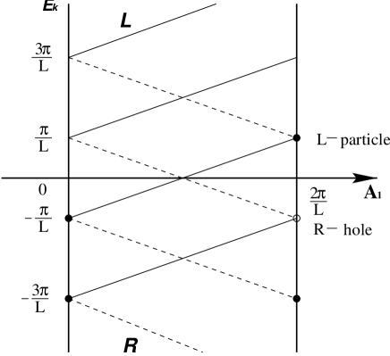
Because the electric charges of the particle and the hole are opposite, the total electric charge vanishes under the change of $A_{1}$:

$$Q(t)=\int dx\ j^{0}(t,x)=Q_{L}+Q_{R}=0,$$ (4.28)

where $Q_{L,R}$ are defined by

$$Q_{L,R}=\int dx\ \bar{\psi}_{L,R}\gamma_{0}\psi_{L,R}=\int dx\ \psi^{\dagger}_{L,R}\psi_{L,R}.$$ (4.29)

Consequently the vector current is conserved. On the contrary, the axial charges can have a non-vanishing value 333In Fujikawa’s method [78], a nontrivial Jacobian appears in the path integral measure of the fermion field when a chiral transformation is performed. Using the eigenstates of the Dirac equation as basis, we can construct the Jacobian which contains the term $$\sum_{n}\psi_{n}^{\dagger}(x)\gamma_{5}\psi_{n}(x),$$ which is equal to the difference of the zero modes of each chirality once the volume integration is performed. The Atiyah-Singer’s index theorem gives the following result: $$\sum_{n,{\rm zero}}\int d^{4}x\ \psi_{n}^{\dagger}(x)\gamma_{5}\psi_{n}(x)=\frac{e^{2}}{16\pi^{2}}\int d^{4}x\ F_{\mu\nu}\tilde{F}^{\mu\nu}$$ in the QED of the (3+1) dimensions. according to its definition:

$$Q_{5}=\int dx\ j_{5}^{0}(t,x)=Q_{L}-Q_{R}=2.$$ (4.30)

We can rewrite this expression as follows:

$$\Delta Q_{5}=\frac{L}{\pi}\Delta A_{1}$$ (4.31)

and per unit time

$$\frac{\Delta Q_{5}}{\Delta t}=\frac{L}{\pi}\frac{\Delta A_{1}}{\Delta t}.$$ (4.32)

Using its definition, we obtain the relation for the axial current

$$\partial_{0}j_{5}^{0}=\frac{1}{\pi}\partial_{0}A_{1}$$ (4.33)

and finally we can write the anomaly for Schwinger’s model in a Lorentz invariant form

$$\partial_{\mu}j_{5}^{\mu}=\frac{1}{\pi}\varepsilon_{\mu\nu}\partial^{\mu}A^{\nu}=\frac{1}{2\pi}\varepsilon_{\mu\nu}F^{\mu\nu}.$$ (4.34)

For the explicit calculation that we will perform in the next chapter, we consider the flavor singlet axial current in QCD. It has the same anomaly equation except for the appropriate group theoretic factor. Applying the same regularization as in the preceding discussion and with gluon fields, $G_{\mu}=\frac{\lambda^{a}}{2}G^{a}_{\mu}$, where $\frac{\lambda^{a}}{2}$’s are the Gell-Mann matrices, the flavor singlet axial current, $A^{0}_{\mu}$, satisfies the following anomaly equation: 444From now on, the notation, $G^{a}_{\mu\nu}$ for the gauge field strength will be used for non-abelian case.

$\displaystyle\partial^{\mu}A_{\mu}^{0}$ $\displaystyle=$ $\displaystyle-\frac{N_{F}\alpha_{s}}{2\pi}\ {\rm Tr}{\bf G}_{\mu\nu}\tilde{\bf G}^{\mu\nu}$ (4.35)
$\displaystyle=$ $\displaystyle-\frac{N_{F}\alpha_{s}}{4\pi}\ \sum_{a}\ G_{\mu\nu}^{a}\tilde{G}^{\mu\nu}_{a},$

where the trace of the Gell-Mann matrices, ${\rm Tr}\bigg{(}\frac{\lambda}{2}\frac{\lambda^{b}}{2}\bigg{)}=\frac{\delta^{ab}}{2},$ has been used in the last line and $N_{F}$ is the flavor number of quark.

4.3 Application of the $U_{A}(1)$ anomaly to the flavor singlet axial charge

As discussed in Chapter 2, the flavor singlet axial anomaly supplies the key to understand the proton spin problem. In this section we give the relation between the flavor singlet axial charge and the singlet axial anomaly. From eq. (4.35) and the fact that $G_{\mu\nu}^{a}\tilde{G}^{\mu\nu}_{a}$ can be written in terms of the Chern-Simons current, $K^{\mu}$ as

$$\frac{1}{2}G_{\mu\nu}^{a}\tilde{G}^{\mu\nu}_{a}=\partial_{\mu}K^{\mu},$$ (4.36)

with the definition of $K^{\mu}$

$$K^{\mu}=\epsilon^{\mu\nu\rho\sigma}G_{\nu}^{a}\bigg{(}G^{a}_{\rho\sigma}-\frac{g_{s}}{3}f_{abc}G_{\rho}^{b}G_{\sigma}^{c}\bigg{)},$$ (4.37)

where $f_{abc}$ is the structure constant of QCD, we can define the following conserved axial vector current for massless quarks (in the chiral limit):

$$\tilde{A}_{\mu}^{0}=A_{\mu}^{0}-N_{F}\frac{\alpha_{s}}{2\pi}K_{\mu}.$$ (4.38)

In the gauge, 555The gluon spin and orbital angular are not separately gauge invariant and hence a choice of gauge is necessary. More detail is given in the next chapter $G^{a}_{0}(x)=0$, the gluon spin spin operator, $\hat{\bf S}^{g}$, becomes

$$\hat{\bf S}^{g}_{i}=-\epsilon_{ijk}G^{j}_{a}\partial^{0}G_{a}^{k}.$$ (4.39)

Moreover, in this gauge, the cubic term vanishes for the spatial components of $K_{\mu}$. Thus, one finds the relation,

$$K_{i}=-\hat{\bf S}^{g}_{i},$$ (4.40)

and its forward proton matrix element,

$$\langle p,S|K^{\mu}|p,S\rangle=-S^{\mu}\Delta g,$$ (4.41)

where $S^{\mu}$ is the proton spin and $\Delta g$ is the net helicity of the gluon along the proton spin.

Due to the conservation of $\tilde{A}_{\mu}^{0}$ in the chiral limit, its forward proton matrix elements are independent of the renormalization scale and the form factor, $\tilde{a}^{0}$, defined through the matrix element

$$\langle p,S|\tilde{A}_{\mu}^{0}|p,S\rangle=\tilde{a}^{0}S_{\mu}$$ (4.42)

should correspond with the value in the quark-model, i.e., $\tilde{a}^{0}=\Delta\Sigma.$ From eq. (4.38) and eq. (4.41), therefore, one has the scale dependent flavor singlet axial charge in terms of $\Delta\Sigma$ and $\Delta g$ as:

$$a^{0}(Q^{2})=\Delta\Sigma-N_{F}\frac{\alpha_{s}}{2\pi}\Delta g(Q^{2}),$$ (4.43)

as given in Chapter 2.

Finally, let’s consider the gauge dependence of the Chern-Simons current. For an abelian case like QED, the gauge transformation,

$$A_{\mu}(x)\rightarrow A_{\mu}(x)+\partial_{\mu}\Lambda(x),$$ (4.44)

induces the change in the Chern-Simon current

$$K_{\mu}(x)\rightarrow K_{\mu}(x)-\frac{1}{2}[\partial_{\mu}\Lambda(x)]\epsilon_{\mu\nu\rho\sigma}F^{\rho\sigma}(x).$$ (4.45)

While the Chern-Simons current changes, its forward proton matrix element (or expectation value) does not since the expectation value of $F^{\rho\sigma}$ vanishes due to the derivatives in the definition of the field strength. Thus, the flavor singlet axial charge is gauge invariant for the abelian case.

On the other hand, for the non-abelian case as in QCD, the situation is more subtle. Under

$$G_{\mu}(x)\rightarrow U(x)G_{\mu}(x)U^{-1}(x)+\frac{i}{g_{s}}(\partial_{\mu}U(x))U^{-1}(x),$$ (4.46)

with the definition, $G_{\mu}=G_{\mu}^{a}\frac{\lambda_{c}^{a}}{2}$, the change of the Chern-Simons current becomes

$\displaystyle K_{\mu}$ $\displaystyle\rightarrow$ $\displaystyle K_{\mu}+\frac{2i}{g_{s}}\epsilon_{\mu\nu\rho\sigma}\partial^{\nu}{\rm Tr}(G^{\alpha}U^{-1}\partial^{\beta}U)$ (4.47)
$\displaystyle+\frac{2}{3g_{s}^{2}}\epsilon_{\mu\nu\rho\sigma}{\rm Tr}\{U^{-1}(\partial^{\nu}U)U^{-1}(\partial^{\alpha}U)U^{-1}(\partial^{\sigma}U)\}.$

The second term is a total divergence so that does not contribute to the forward proton matrix element. Although the third term can also be shown to be a divergence [79], but it cannot be discarded because of the non-trivial topological structure [80] of QCD. As a result, its forward proton matrix element is not gauge invariant. To avoid these problems in our discussion, we will treat gluons as abelianized fields in the next discussions.

4.4 Color anomaly in the chiral bag model [34] [16]

In the previous chapter, the boundary conditions for the confined gluons in the chiral bag model have been given as

$$\hat{\bf r}\cdot{\bf E}^{a}=0,\hskip 28.45274pt\hat{\bf r}\times{\bf B}^{a}=0$$ (4.48)

with $\hat{\bf r}$ the outward unit vector normal to the bag surface and $a$ the color index. These conditions mean that the color electric fields, ${\bf E}^{a}$, point along the surface, while the color magnetic fields, ${\bf B}^{a}$, are orthogonal to the surface. These are the usual MIT bag boundary conditions. We will show that the leakage of the color charge resulting from the $\eta^{\prime}$ field at the bag surface, as discussed at the beginning of this chapter, makes these boundary conditions change. As a result, the color electric field has a component normal to the bag surface and the color magnetic field a component along the surface.

The boundary condition for the quarks due to $\eta^{\prime}$ field at the bag surface is given by

$$(i\mbox{\boldmath$\gamma$}\cdot\hat{\bf r}+e^{i\gamma_{5}\eta(\beta)})\psi=0,$$ (4.49)

where $\eta=\eta^{\prime}/f_{\eta^{\prime}}\equiv\eta^{\prime}/f_{0}$ and $\beta$ is a point on the surface. At the classical level this boundary condition makes the color current of the quark, confined inside the bag, to have no leakage outside. As a result, the color charge of the bag is a constant in time,

$\displaystyle\langle 0|\dot{Q}^{a}|0\rangle$ $\displaystyle=$ $\displaystyle-\int_{\Sigma}d\beta\ \langle 0|{\bf j}^{a}\cdot\hat{\bf r}|0\rangle$ (4.50)
$\displaystyle=$ $\displaystyle-g_{s}\oint_{\Sigma}d\beta\ \langle 0|\ \bar{\psi}\mbox{\boldmath$\gamma$}\cdot\hat{\bf r}\frac{\lambda^{a}}{2}\psi\ |0\rangle=0,$

where we have made use of the quasi-abelian approximation for simplicity and $\Sigma=\partial B$. Once the calculation is completed, we will extract the non-abelian structure by inspection.

The quantum correction to $\dot{Q}^{a}$ due to the $\eta$ can be obtained by introducing the gauge invariant point-splitting regularization to the color current operator as before. If we use a point-splitting in time direction and choose the temporal gauge condition, $G_{0}^{a}=0$, the regularized color current operator in the quasi-abelian approximation at the surface becomes

$\displaystyle{\bf j}^{a}_{\rm reg}(\beta)$ $\displaystyle=$ $\displaystyle g_{s}\bar{\psi}(\beta+\epsilon/2)\mbox{\boldmath$\gamma$}\ \frac{\lambda^{a}}{2}\exp\bigg{(}ig_{s}\int_{\beta-\frac{1}{2}\epsilon}^{\beta+\frac{1}{2}\epsilon}dz^{\mu}G_{\mu}(z)\bigg{)}\psi(\beta-\epsilon/2)$ (4.51)
$\displaystyle=$ $\displaystyle g_{s}\bar{\psi}(\beta+\epsilon/2)\mbox{\boldmath$\gamma$}\ \frac{\lambda^{a}}{2}\psi(\beta-\epsilon/2).$

Then, we have

$$\dot{Q}^{a}\equiv\langle 0|\dot{Q}^{a}|0\rangle=-g_{s}\lim_{\epsilon\rightarrow 0}\oint_{\Sigma}d\beta\ \langle 0|\ \bar{\psi}(\beta+\epsilon/2)\mbox{\boldmath$\gamma$}\cdot\hat{\bf r}\frac{\lambda^{a}}{2}\psi(\beta-\epsilon/2)\ |0\rangle$$ (4.52)

as the regularized expression. Using the boundary condition, eq. (4.49), the effect of the $\eta$ appears explicitly as

$\displaystyle\dot{Q}^{a}$ $\displaystyle=$ $\displaystyle g_{s}\lim_{\epsilon\rightarrow 0}\oint_{\Sigma}d\beta\ \langle 0|\ \bar{\psi}(\beta+\epsilon/2)\mbox{\boldmath$\gamma$}\cdot\hat{\bf r}\frac{\lambda^{a}}{2}e^{-i\gamma_{5}\eta(\beta+\epsilon/2)}e^{i\gamma_{5}\eta(\beta-\epsilon/2)}\psi(\beta-\epsilon/2)\ |0\rangle$ (4.53)
$\displaystyle=$ $\displaystyle-i\frac{g_{s}}{2}\lim_{\epsilon\rightarrow 0}\epsilon\oint_{\Sigma}d\beta\ \langle 0|\ \bar{\psi}(\beta+\epsilon/2)\mbox{\boldmath$\gamma$}\cdot\hat{\bf r}\frac{\lambda^{a}}{2}\gamma_{5}\psi(\beta-\epsilon/2)\ |0\rangle\dot{\eta}(\beta),$

where the relation

$\displaystyle e^{-i\gamma_{5}\eta(\beta+\epsilon/2)}e^{i\gamma_{5}\eta(\beta-\epsilon/2)}$ $\displaystyle=$ $\displaystyle e^{-i\gamma_{5}(\eta(\beta+\epsilon/2)-\eta(\beta-\epsilon/2))}e^{-\frac{1}{2}[\eta(\beta+\epsilon/2),\ \eta(\beta-\epsilon/2)]}$ (4.54)
$\displaystyle\simeq$ $\displaystyle 1-i\gamma_{5}\dot{\eta}(\beta)\epsilon$

up to $O(\epsilon)$, and point splitting in the time direction, have been used. Rewriting the vacuum expectation values in terms of the components gives

$$\dot{Q}^{a}=-i\frac{g_{s}}{2}\lim_{\epsilon\rightarrow 0}\epsilon\oint_{\Sigma}d\beta\ {\rm Tr}\bigg{(}\gamma_{5}\vec{\gamma}\cdot\hat{\bf r}\frac{\lambda^{a}}{2}S^{+}(\beta-\epsilon/2;\beta+\epsilon/2)\bigg{)}\dot{\eta}(\beta),$$ (4.55)

where $S^{+}(\beta,\beta^{\prime})$ is defined by

$$S^{+}(\beta,\beta^{\prime})=\lim_{(x,x^{\prime})\rightarrow(\beta,\beta^{\prime})}S(x,x^{\prime})$$ (4.56)

from the confined fermion propagator $S(x,x^{\prime})$. The multiple reflection expansion method [81] produces the relation

$$S^{+}(\beta-\epsilon/2;\beta+\epsilon/2)=\frac{1}{4}(1+\mbox{\boldmath$\gamma$}_{E}\cdot\hat{\bf r}U_{5})S(\beta-\epsilon/2;\beta+\epsilon/2)(3-U_{5}\mbox{\boldmath$\gamma$}_{E}\cdot\hat{\bf r})$$ (4.57)

in Euclidean space. 666The $\gamma$ matrices of Euclidean space are related to those of Minkowski space according to the rules: ${\bf x}_{E}={\bf x},x_{4}=ix_{0},\mbox{\boldmath$\gamma$}_{E}=-i\mbox{\boldmath$\gamma$},\gamma_{4}=\gamma_{0},\ {\rm and}\ \gamma_{5}=-\gamma^{1}_{E}\gamma^{2}_{E}\gamma^{3}_{E}\gamma^{4}$ so that all $\gamma_{\mu}$ become the hermitian matrices. The boundary conditions for the quark due to $\eta$ becomes $$\mbox{\boldmath$\gamma$}_{E}\cdot\hat{\bf r}\psi=U_{5}\psi\ \ {\rm and}\ \ \bar{\psi}\mbox{\boldmath$\gamma$}_{E}\cdot\hat{\bf r}=-\bar{\psi}U_{5}.$$ From these, the confined fermion propagator satisfies the boundary conditions $$U_{5}(\alpha)S(\alpha,x^{\prime})=\mbox{\boldmath$\gamma$}_{E}\cdot\hat{\bf r}S(\alpha,x^{\prime})\ \ {\rm and}\ \ S(x,\alpha)U_{5}(\alpha)=-S(x,\alpha)\mbox{\boldmath$\gamma$}_{E}\cdot\hat{\bf r}$$ for any vector $\alpha$ on the boundary. Here $U_{5}=e^{i\gamma_{5}\eta}$. Assuming that $\eta$ on the bag surface does not depend on the location, but only on time, 777One can generalize the result to a variation with a space-time dependent $\eta(x,t)$ by replacing the ordinary derivative by a functional derivative. we have

$\displaystyle\frac{dQ^{a}}{d\eta}$ $\displaystyle=$ $\displaystyle-i\frac{g_{s}}{2}\lim_{\epsilon\rightarrow 0}\epsilon\oint_{\Sigma}d\beta\ {\rm Tr}\bigg{(}\gamma_{5}\mbox{\boldmath$\gamma$}\cdot\hat{\bf r}\frac{\lambda^{a}}{2}S^{+}(\beta-\epsilon/2;\beta+\epsilon/2)\bigg{)}$ (4.58)
$\displaystyle=$ $\displaystyle\frac{g_{s}}{2}\lim_{\epsilon\rightarrow 0}\epsilon\oint_{\Sigma}d\beta_{E}\ {\rm Tr}\bigg{(}\gamma_{5}\frac{\lambda^{a}}{2}(\mbox{\boldmath$\gamma$}_{E}\cdot\hat{\bf r}+U_{5})S(\beta-\epsilon/2;\beta+\epsilon/2)\bigg{)}$
$\displaystyle=$ $\displaystyle g_{s}\lim_{\epsilon\rightarrow 0}\epsilon\int_{\Sigma}d\beta_{E}\ {\rm Tr}\bigg{(}\gamma_{5}\frac{\lambda^{a}}{2}\mbox{\boldmath$\gamma$}_{E}\cdot\hat{\bf r}S(\beta-\epsilon/2;\beta+\epsilon/2)\bigg{)}.$

Here the eq. (4.57) and the boundary condition of the confined propagator in the footnote have been used in order to get the last result. Because of the structure of the $\gamma$ matrices in eq. (4.58) the singular contribution arises from the first order term in the gluon interaction in the perturbative expansion of the confined fermion propagator. In the Minkowski space the confined fermion propagator is

$$S(\beta-\epsilon/2;\beta+\epsilon/2)\sim\int_{B}d^{4}x\ S_{0}(\beta-\epsilon/2-x)(-ig_{s}\gamma\cdot G^{b}(x)\lambda^{b}/2)S_{0}(x-\beta-\epsilon/2),$$ (4.59)

where $S_{0}(x,x^{\prime})$ is the free fermion propagator. Substituting this result into the eq. (4.58) leads to the integral in momentum space,

$\displaystyle\frac{dQ^{a}}{d\eta}$ $\displaystyle=$ $\displaystyle-ig_{s}\lim_{\epsilon\rightarrow 0}\epsilon\oint_{\Sigma}d\beta\ {\rm Tr}\bigg{(}\gamma_{5}\mbox{\boldmath$\gamma$}\cdot\hat{\bf r}\frac{\lambda^{a}}{2}S(\beta-\epsilon/2;\beta+\epsilon/2)\bigg{)}$ (4.60)
$\displaystyle=$ $\displaystyle g_{s}^{2}\lim_{\epsilon\rightarrow 0}\epsilon\oint_{\Sigma}d\beta\ {\rm Tr}\bigg{(}\gamma_{5}\mbox{\boldmath$\gamma$}\cdot\hat{\bf r}\frac{\lambda^{a}}{2}\frac{\lambda^{b}}{2}\int(dq)\ G^{b}_{\alpha}(q)e^{iq\cdot(\beta+\epsilon/2)}$
$\displaystyle\hskip 99.58464pt\cdot\ \int(dp)\frac{1}{\not p}\gamma^{\alpha}\frac{1}{\not p-\not q}e^{ip\cdot\epsilon}\bigg{)}.$

From the relations

$${\rm Tr}(\gamma^{5}\gamma^{i}\gamma^{\beta}\gamma^{\alpha}\gamma^{\sigma})=-4i\epsilon^{i\beta\alpha\sigma},\hskip 28.45274pt{\rm Tr}\bigg{(}\frac{\lambda^{a}}{2}\frac{\lambda^{b}}{2}\bigg{)}=\frac{\delta^{ab}}{2}$$ (4.61)

and the fact that for the limit $\epsilon\rightarrow 0$ the integral over $p$ becomes

$$\int(dp)\frac{p_{\beta}}{p^{4}}e^{ip\cdot\epsilon}=-\frac{1}{8\pi^{2}}\frac{\epsilon_{\beta}}{\epsilon^{2}},$$ (4.62)

we arrive at the final result in the form of a surface integral

$$\frac{dQ^{a}}{d\eta}=-\frac{g_{s}^{2}}{4\pi^{2}}\epsilon^{0i\alpha\sigma}\oint_{\Sigma}d\beta\ \hat{\bf r}_{i}\partial_{\alpha}G^{a}_{\sigma}(\beta).$$ (4.63)

We can write this result in terms of the color magnetic fields in the quasi–abelian case as:

$$\frac{dQ^{a}}{d\eta}=N_{F}\frac{g_{s}^{2}}{4\pi^{2}}\oint_{\partial B}d\beta\ {\bf B}^{a}\cdot\hat{\bf r},$$ (4.64)

when there are $N_{F}$ massless quarks. Note that eq. (4.64) has been obtained with unconstraint radiated gluon. Since we consider a confine theory, there should be the additional factor of 1/2 in the final result by making gluon confined only inside the bag. Then, the result becomes

$$\frac{dQ^{a}}{d\eta}=N_{F}\frac{g_{s}^{2}}{8\pi^{2}}\oint_{\partial B}d\beta\ {\bf B}^{a}\cdot\hat{\bf r}.$$ (4.65)

Eq. (4.65) means that color charge disappears from the bag due to the time variation of the $\eta$ field which is the artifact of the effective approach as ours. In other words, the color charge confined at the classical level leaks out at the quantum level. A simple way to remedy this problem is to introduce a surface term of the following type as a counter term in the action to remove the artifact:

$$S_{\rm CT}\sim-N_{F}\frac{g_{s}^{2}}{8\pi^{2}}\oint_{\partial B}d\beta\ G_{0}^{a}{\bf B}^{a}\cdot\hat{\bf r}\eta(\beta).$$ (4.66)

Chiral invariance, covariance, and general gauge transformation properties allow us to rewrite eq. (4.66) in a general form

$$S_{\rm CT}=i\frac{g_{s}^{2}}{32\pi^{2}}\oint_{\partial B}d\beta\ K^{\mu}n_{\mu}{\rm Tr}({\rm ln}U^{\dagger}-{\rm ln}U),$$ (4.67)

where $K^{\mu}$ is the Chern-Simons current defined by

$$K^{\mu}=\epsilon^{\mu\nu\alpha\beta}\bigg{(}G^{a}_{\nu}G^{a}_{\alpha\beta}-\frac{1}{3}g_{s}f^{abc}G^{a}_{\nu}G^{b}_{\alpha}G^{c}_{\beta}\bigg{)}$$ (4.68)

and $n_{\mu}$ is the outward unit four vector normal to the bag surface. Here, $U=e^{i\eta^{\prime}/f_{0}}e^{i\pi/f}$ as given in the previous chapter. This counter term describes that the colorless $\eta$ field outside the bag interacts with gluons at the bag surface by the help of quarks. We expect that this term may be generated naturally in the effective action of the chiral bag model as the interaction term between the neutral pion and photons in the effective action of QED [82].

Note that eq. (4.67) is not gauge invariant on the bag surface because of the Chern-Simons current. Thus at the classical level, the Lagrangian is not gauge invariant. However, at the quantum level, the invariance is restored by the cancellation between the anomalous term, eq. (4.65), and the surface term, eq. (4.67).

Including this color anomaly phenomenon, the action for the chiral bag given in the previous chapter is generalized to

$\displaystyle S$ $\displaystyle=$ $\displaystyle S_{B}+S_{\bar{B}}+S_{\partial B}$
$\displaystyle S_{B}$ $\displaystyle=$ $\displaystyle\int_{B}d^{4}x\bigg{(}\bar{\psi}i\not D\psi-\frac{1}{2}{\rm Tr}G_{\mu\nu}G^{\mu\nu}\bigg{)},$
$\displaystyle S_{\bar{B}}$ $\displaystyle=$ $\displaystyle\frac{f_{\pi}^{2}}{4}\int_{\bar{B}}\bigg{(}{\rm Tr}\partial_{\mu}U^{\dagger}\partial^{\mu}U+\frac{1}{4N_{F}}m_{\eta^{\prime}}^{2}[{\rm Tr}({\rm ln}U^{\dagger}-{\rm ln}U)]^{2}\bigg{)}+\cdots+S_{WZW},$
$\displaystyle S_{\partial B}$ $\displaystyle=$ $\displaystyle\frac{1}{2}\oint_{\partial B}d\Sigma^{\mu}\left\{n_{\mu}\bar{\psi}U_{5}\psi+i\frac{g_{s}^{2}}{16\pi^{2}}K_{\mu}{\rm Tr}({\rm ln}U^{\dagger}-{\rm ln}U)\right\}.$ (4.69)

From the presence of the Chern-Simons term in the surface action, the boundary conditions for gluon fields at classical level are affected. In place of the MIT conditions eq. (4.48), we have instead

$\displaystyle\hat{\bf r}\cdot{\bf E}^{a}$ $\displaystyle=$ $\displaystyle-\frac{N_{F}g_{s}^{2}}{8\pi^{2}f_{0}}\hat{\bf r}\cdot{\bf B}^{a}\eta^{\prime},$
$\displaystyle\hat{\bf r}\times{\bf B}^{a}$ $\displaystyle=$ $\displaystyle\frac{N_{F}g_{s}^{2}}{8\pi^{2}f_{0}}\hat{\bf r}\times{\bf E}^{a}\eta^{\prime}.$ (4.70)

The fact that the color electric field can have a radial component contrary to the MIT conditions plays an important role on the proton spin problem. Besides, the $\eta^{\prime}$ mass can be estimated by using these boundary conditions and the axial anomaly [83].

Chapter 5 Flavor singlet axial charge in the chiral bag model

In this chapter, we present the calculation of the Flavor Singlet Axial Charge (FSAC) in the chiral bag model scenario and demonstrate how the Cheshire Cat Principle [15, 16] operates for the observables that are not topological as baryon charge discussed in a previous chapter. In order to do so we need a specific formulation of the model through its equations of motion and boundary conditions. We should stress that although we are truncating the model, the model itself is quite general and represents low-energy dynamics of QCD.

We recall that the equations of motion have been shown in Chapter 3 and the color boundary conditions have been introduced in Chapter 4. Our calculation will be carried out in the static spherical cavity approximation, that is, our bag, polarized along $z-$direction, is a static sphere of radius $R$ dividing two regions of space in which the theory is implemented by QCD for $r<R$, and by an effective meson theory for $r>R$. Besides, we treat, throughout the calculation, the gluons as abelian fields, i.e., we work in the lowest order approximation to QCD in perturbation theory.

First we calculate the various static contributions to this observable, and then, after considering the gluon spin, we proceed to include the Casimir contribution which arises due to the change in the boundary conditions of gluons associated to the color anomaly.

5.1 The formalism

To obtain the FSAC, we need to calculate the matrix elements of the flavor singlet axial current. According to the Cheshire Cat Principle (CCP) discussed in Chapter 3, the flavor singlet current appears in the chiral bag model as the sum of two terms, one coming from the interior of the bag and the other from the outside, populated among others by the $\eta^{\prime}-$meson 111From now on we will omit the prime and write simply $\eta$ for this meson.

$$A^{0}_{\mu}=A^{0}_{\mu,B}\Theta_{B}+A^{0}_{\mu,\bar{B}}\bar{\Theta}_{B}.$$ (5.1)

Here, $\Theta_{B}$ and $\bar{\Theta}_{B}$ are defined, as before, as $\Theta_{B}=\theta(R-r)$ and $\bar{\Theta}_{B}=1-\Theta_{B}$, with $R$ being the radius of the bag. We demand that the $U_{A}(1)$ anomaly is given in the model by

$$\partial_{\mu}A^{0}_{\mu}=-\frac{\alpha_{s}N_{F}}{4\pi}\sum_{a}G_{\mu\nu}^{a}\tilde{G}^{\mu\nu,a}\Theta_{B}+2f_{\pi}m_{\eta}^{2}\eta\bar{\Theta}_{B}.$$ (5.2)

Our task is to construct a FSAC in the chiral bag model that is gauge-invariant and consistent with this anomaly equation. Our basic assumption is that in the nonperturbative sector outside of the bag, the only relevant $U_{A}(1)$ degree of freedom is the massive $\eta$ field. This assumption allows us to write

$$A^{0}_{\mu,\bar{B}}=A^{0}_{\mu,\eta}=2f_{\pi}\partial^{\mu}\eta$$ (5.3)

with its divergence given by

$$\partial^{\mu}A^{0}_{\mu,\eta}=2f_{\pi}m_{\eta}^{2}\eta.$$ (5.4)

The immediate question to ask is: what is the gauge-invariant and regularized $A^{0}_{\mu,B}$ such that the anomaly equation, eq. (5.2), is satisfied? To address this question, we rewrite the current, eq. (5.1), absorbing the theta functions, as

$$A^{0}_{\mu}=A^{0}_{\mu,B_{Q}}+A^{0}_{\mu,B_{G}}+A^{0}_{\mu,\eta}$$ (5.5)

such that

$\displaystyle\partial^{\mu}(A^{0}_{\mu,B_{Q}}+A^{0}_{\mu,\eta})$ $\displaystyle=$ $\displaystyle 2f_{\pi}m_{\eta}^{2}\eta\bar{\Theta}_{B},$ (5.6)
$\displaystyle\partial^{\mu}A^{0}_{\mu,B_{G}}$ $\displaystyle=$ $\displaystyle\frac{\alpha_{s}N_{F}}{\pi}\sum_{a}{\bf E}^{a}\cdot{\bf B}^{a}\Theta_{B},$ (5.7)

where the relation $G_{\mu\nu}^{a}\tilde{G}^{\mu\nu,a}=-4{\bf E}^{a}\cdot{\bf B}^{a}$ has been used. The sub-indices $Q$ and $G$ signal that these currents are written in terms of quark and gluon fields respectively. In writing eq. (5.6), we have ignored the up and down quark masses. Going to the static situation, appropriate to our discussion, eq. (5.7) can be written as

$$\mbox{\boldmath$\nabla$}\cdot{\bf A}^{0}_{B_{G}}=\frac{\alpha_{s}N_{F}}{\pi}\sum_{a}{\bf E}^{a}\cdot{\bf B}^{a}\Theta_{B}.$$ (5.8)

We should stress that since we are dealing with an interacting theory, there is no unique way to separate the different contributions from the gluon, quark and $\eta$ components. In particular, the separation we adopt, (5.6) and (5.7), is non-unique although the sum is free of ambiguities. We find, however, that this separation leads to a natural partition of the contributions in the framework of the bag description for confinement we use.

5.2 The quark contribution

The quark current is given by

$$A^{\mu}_{B_{Q}}=\bar{\psi}\gamma^{\mu}\gamma_{5}\psi$$ (5.9)

where $\psi$ should be understood to be the bagged quark field, which means that the quark field is a cavity mode before turning on the quark-gluon interaction. The quark current contribution to the FSAC is given by

$$a^{0}_{B_{Q}}=\langle{\rm P}|\int_{B}d^{3}r\bar{\psi}\gamma_{3}\gamma_{5}\psi\ |{\rm P}\rangle$$ (5.10)

with the proton state, $|{\rm P}\rangle$, given by eq. (3.116).

The calculation of this type of matrix elements in the chiral bag model is nontrivial due to the baryon charge leakage between the interior and the exterior through the Dirac sea. But we know how to do this in an unambiguous way. A complete account of such calculations can be found in [22, 32, 33]. The leakage produces an $R$ dependence, as shown in Fig. 5.1, which would otherwise not be there in the matrix element, eq. (5.10). It is worth stressing that, as seen in the Fig. 5.1, for zero radius, that is, in the pure skyrmion scenario for the proton this matrix element vanishes. The contribution grows as a function of $R$ towards the pure MIT result that technically is reached for infinite radius. The result of this calculation was presented in refs. [22, 21]. No new ingredient has been added.

Refer to caption

Figure 5.1: Various contributions to the flavor singlet axial current of the proton as a function of bag radius : (a) quark contribution $a^{0}_{B_{Q}}$; (b) $\eta^{\prime}$ contribution $a^{0}_{\eta}$ and (c) the sum.

5.3 The meson current $A^{\mu}_{\eta}$

We can get the $\eta$ field contribution in terms of the quark contribution. From the boundary condition eq. (3.156) for the $\eta$ field,

$$\langle{\rm P}|\ \hat{\bf r}\cdot(\bar{\psi}\mbox{\boldmath$\gamma$}\gamma_{5}\psi)\ |{\rm P}\rangle=\langle{\rm P}|\ \hat{\bf r}\cdot(2f_{\pi}\mbox{\boldmath$\nabla$}\eta)\ |{\rm P}\rangle,\hskip 14.22636pt{\rm at}\ r=R,$$ (5.11)

and the fact that the bagged current, $\bar{\psi}\mbox{\boldmath$\gamma$}\gamma_{5}\psi$, is divergenceless for massless quarks, we have the following identity:

$$\langle{\rm P}|\int_{\partial B}d^{2}s\ \hat{\bf r}\cdot(r_{3}2f_{\pi}\mbox{\boldmath$\nabla$}\eta)\ |{\rm P}\rangle=\langle{\rm P}|\int_{B}d^{3}r(\bar{\psi}\gamma_{3}\gamma_{5}\psi)\ |{\rm P}\rangle.$$ (5.12)

Substituting $\eta$ field given by

$$\eta=C{\bf S}\cdot\mbox{\boldmath$\nabla$}\bigg{(}\frac{e^{-m_{\eta}r}}{r}\bigg{)},$$ (5.13)

where ${\bf S}$ is the proton spin operator, into the left hand side leads to

$$\langle{\rm P}|\int_{\partial B}d^{2}s\ \hat{\bf r}\cdot(r_{3}2f_{\pi}\mbox{\boldmath$\nabla$}\eta)\ |{\rm P}\rangle=Cf_{\pi}\frac{8\pi}{3}S_{3}[2(1+y_{\eta})+y_{\eta}^{2}]e^{-y_{\eta}}.$$ (5.14)

Here

$$y_{\eta}\equiv m_{\eta}R.$$ (5.15)

Therefore $C$ is determined by

$$C=\frac{3}{4\pi f_{\pi}}[2(1+y_{\eta})+y_{\eta}^{2}]e^{y_{\eta}}\langle{\rm P}|\int_{B}d^{3}r(\bar{\psi}\gamma_{3}\gamma_{5}\psi)\ |{\rm P}\rangle.$$ (5.16)

Consequently, the $\eta$ contribution becomes

$$a^{0}_{\eta}=\langle{\rm P}|\int_{\bar{B}}d^{3}r2f_{\pi}\mbox{\boldmath$\nabla$}_{3}\eta\ |{\rm P}\rangle=\frac{1+y_{\eta}}{2(1+y_{\eta})+y_{\eta}^{2}}\langle{\bf P}|\int_{B}d^{3}r\bar{\psi}\gamma_{3}\gamma_{5}\psi\ |{\bf P}\rangle.$$ (5.17)

Thus we have the result that the $\eta$ contribution outside is entirely given in terms of the quark contribution inside and the $\eta$ mass.

In Fig. 5.1 we show the radial dependence of several contributions. We show the results of [22, 21], which arise from the charge leakage mechanism, and follow the quark distribution. We show also the contribution of the $\eta$ just calculated, by taking the quark current matrix element also from [22, 21]. Since the $\eta$ field has no topological structure, its contribution vanishes in the skyrmion limit. Our calculation illustrates how the dynamics of the exterior can be mapped onto that of the interior by the boundary conditions. We may summarize the analysis of these two contributions by stating that no trace of the CCP is apparent in Fig. 5.1. Thus if the CCP is to emerge, the only possibility one foresees, is that the gluons do the miracle!

5.4 The gluon current $A^{\mu}_{B_{G}}$

Understanding the FSAC and its implications in the present framework involves crucially the role of the gluon contribution, in particular its static properties and vacuum fluctuations, i.e., the Casimir effects. The calculation of the Casimir effects in the next section constitutes the principal aim of this work.

Since we have assigned the anomaly to the gluon fields, eq. (5.7), the gluonic axial current has the form

$$A^{0}_{\mu,B_{G}}=\frac{N_{F}\alpha_{s}}{4\pi}\epsilon_{\mu\nu\rho\lambda}A^{\nu a}(G^{\rho\lambda a}-\frac{1}{3}g_{s}f^{abc}A^{\rho b}A^{\lambda c}).$$ (5.18)

Note that this expression is not locally gauge invariant. In fact there is no gauge invariant dimension-3 vector operator with the gauge field alone.

With this gluonic axial current, the boundary condition, eq. (5.11), changes to

$$\langle{\rm P}|\ \hat{\bf r}\cdot({\bf A}^{0}_{B_{Q}}+{\bf A}^{0}_{B_{G}})\ |{\rm P}\rangle=\langle{\rm P}|\ \hat{\bf r}\cdot(2f_{\pi}\mbox{\boldmath$\nabla$}\eta)\ |{\rm P}\rangle,\hskip 14.22636pt{\rm at}\ r=R.$$ (5.19)

Using this boundary condition and the anomaly, eq. (5.8), the total FSAC of the proton can be constructed. Since the quark is a divergenceless field, we rewrite eq. (5.8) in the form

$$\mbox{\boldmath$\nabla$}\cdot({\bf A}^{0}_{B_{Q}}+{\bf A}^{0}_{B_{G}})=N_{F}\frac{\alpha_{s}}{\pi}\sum_{a}{\bf E}^{a}\cdot{\bf B}^{a}\Theta_{B}.$$ (5.20)

Integrating this equation with respect to the bag volume after multiplying ${\bf r}$, the matrix element for proton becomes

$\displaystyle\langle{\rm P}|\int_{B}d^{3}r({\bf A}^{0}_{B_{Q}}+{\bf A}^{0}_{B_{G}})\ |{\rm P}\rangle=-\langle{\rm P}|N_{F}\frac{\alpha_{s}}{\pi}\int_{B}d^{3}r\ \sum_{a}{\bf E}^{a}\cdot{\bf B}^{a}{\bf r}\ |{\rm P}\rangle$
$\displaystyle\hskip 150.79968pt+\langle{\rm P}|\int_{\partial B}d\mbox{\boldmath$\Sigma$}\cdot({\bf A}^{0}_{B_{Q}}+{\bf A}^{0}_{B_{G}}){\bf r}\ |{\rm P}\rangle.$ (5.21)

Using the boundary condition, eq. (5.19), we see that the second term yields the contribution from $\eta$ outside the bag. Therefore, we have

$\displaystyle\langle{\rm P}|\int_{B}d^{3}r({\bf A}^{0}_{B_{Q}}+{\bf A}^{0}_{B_{G}})+\int_{\bar{B}}d^{3}r{\bf A}^{0}_{\eta}\ |{\rm P}\rangle=-\langle{\rm P}|N_{F}\frac{\alpha_{s}}{\pi}\int_{B}d^{3}r\ \sum_{a}{\bf E}^{a}\cdot{\bf B}^{a}{\bf r}\ |{\rm P}\rangle$
$\displaystyle\hskip 179.25244pt-\langle{\rm P}|\int_{\bar{B}}d^{3}r(2f_{\pi}m_{\eta}^{2}\eta){\bf r}\ |{\rm P}\rangle,$ (5.22)

and, since there is no explicit coupling between gluons and the $\eta$ field at the tree level in the model Lagrangian, the first term on the right-hand side of the above equation may be considered as the gluonic contribution to the FSAC, namely

$$a^{0}_{G}=\langle{\rm P}|-\frac{N_{F}\alpha_{s}}{\pi}\int_{B}d^{3}r\ r_{3}\ \sum_{a}{\bf E}^{a}\cdot{\bf B}^{a}\ |{\rm P}\rangle.$$ (5.23)

This corresponds to the second term in eq. (4.43) in Chapter 4.

Let us proceed to calculate the gluonic contribution. We begin by dividing the gluon current into two terms according to their origin

$$A^{\mu}_{B_{G}}=A^{\mu}_{G,stat}+A^{\mu}_{G,vac}.$$ (5.24)

The first term arises from the quark and $\eta$ sources, while the second is associated with the properties of the vacuum of the model. One might worry that this contribution cannot be split in these two terms without double counting. That there is no cause for worry can be seen in several ways. Technically, it is easy to show it in terms of mode creation and annihilation operators. One can also show this intuitively by making the analogy to the condensate expansion in QCD [84], where the perturbative terms and the vacuum condensates enter additively to the lowest order.

Let us first describe the static term which effectively accounts for the mixing of the light quarks with the ${\bf E}^{a}\cdot{\bf B}^{a}$ of the anomaly. The boundary conditions for the gluon field corresponds in our approaximation to the original MIT one [10]. The source for it is the quark current that appears in the equations of motion after performing a perturbative expansion in the QCD coupling constant, i.e., the quark color current

$$g_{s}{\bar{\psi}}\gamma_{\mu}\lambda^{a}\psi$$ (5.25)

where the $\psi$ fields represent the lowest cavity modes. In this lowest mode approximation, the color electric and magnetic fields are given by

$${\bf E}^{a}=g_{s}\frac{\lambda^{a}}{4\pi}\frac{\hat{\bf r}}{r^{2}}\rho(r)$$ (5.26)
$${\bf B}^{a}=g_{s}\frac{\lambda^{a}}{4\pi}\left\{\frac{\mu(r)}{r^{3}}(3\hat{\bf r}\mbox{\boldmath$\sigma$}\cdot\hat{\bf r}-\mbox{\boldmath$\sigma$})+\bigg{(}\frac{\mu(R)}{R^{3}}+2M(r)\bigg{)}\mbox{\boldmath$\sigma$}\right\}$$ (5.27)

where $\rho$ is related to the quark density $\rho^{\prime}$ as222Note that the quark density that appears here is associated with the color charge, not with the quark number (or rather the baryon charge) that leaks due to the hedgehog pion.

$$\rho(r,\Gamma)=\int_{\Gamma}^{r}ds\rho^{\prime}(s)$$

and $\mu,M$ to the vector current density

$\displaystyle\mu(r)$ $\displaystyle=$ $\displaystyle\int_{0}^{r}ds\mu^{\prime}(s),$
$\displaystyle M(r)$ $\displaystyle=$ $\displaystyle\int_{r}^{R}ds\frac{\mu^{\prime}(s)}{s^{3}}.$

As considered in Chapter 3, the lower limit $\Gamma$ is taken to be zero in the MIT bag model $-$ in which case the boundary condition is satisfied only globally, that is, after averaging $-$ and $\Gamma=R$ in the so called monopole solution [22, 23] $-$ in which case, the boundary condition is satisfied locally.

Now we introduce the $\eta$ field. We perform the same calculation however with the color anomaly boundary conditions given in Chapter 4,

$$\hat{\bf r}\cdot{\bf E}^{a}=-\frac{N_{F}g_{s}^{2}}{8\pi^{2}f_{0}}\hat{\bf r}\cdot{\bf B}^{a}\eta(R),\hskip 28.45274pt\hat{\bf r}\times{\bf B}^{a}=\frac{N_{F}g_{s}^{2}}{8\pi^{2}f_{0}}\hat{\bf r}\times{\bf E}^{a}\eta(R).$$ (5.28)

In the approximation of keeping the lowest non-trivial term, the boundary conditions become

$$\hat{\bf r}\cdot{\bf E}_{stat}^{a}=-\frac{N_{F}g_{s}^{2}}{8\pi^{2}f_{0}}\hat{\bf r}\cdot{\bf B}^{a}_{g}\eta(R)$$ (5.29)
$$\hat{\bf r}\times{\bf B}_{stat}^{a}=\frac{N_{F}g_{s}^{2}}{8\pi^{2}f_{0}}\hat{\bf r}\times{\bf E}^{a}_{g}\eta(R).$$ (5.30)

Here ${\bf E}^{a}_{g}$ and ${\bf B}^{a}_{g}$ are the lowest order fields [22, 23] given by (5.26) and (5.27) and $\eta(R)$ is the $\eta$-meson field at the boundary. The $\eta$ field is given by

$$\eta({\bf r})=-\frac{g_{NN\eta}}{4\pi M}{\bf S}\cdot\hat{\bf r}\frac{1+m_{\eta}r}{r^{2}}e^{-m_{\eta}r}$$ (5.31)

where the coupling constant is determined from the surface conditions, eq. (5.16), the results of refs. [22, 23] and this expression for the $\eta$.

Note that the magnetic field is not affected by the new boundary conditions, since ${\bf E}^{a}_{g}$ points into the radial direction. The effect on the electric field is just a change in the charge, i.e.,

$$\rho_{stat}(r)=\rho(r,\Gamma)+\rho_{\eta}(R)$$ (5.32)

where

$$\rho_{\eta}(R)=\frac{N_{F}g_{s}^{2}}{64\pi^{3}M}\frac{g_{NN\eta}}{f}(1+y_{\eta})e^{-y_{\eta}}.$$ (5.33)

The contribution to the FSAC arising from these fields is determined from the expectation value of the anomaly

$$a^{0}_{G,stat}=\langle{\rm P}|-\frac{N_{F}\alpha_{s}}{\pi}\int_{B}d^{3}r\ r_{3}\ {\bf E}^{a}_{stat}\cdot{\bf B}^{a}_{stat}|{\rm P}\rangle.$$ (5.34)

The result of this contribution appears in Fig. 5.2 , where we show the MIT solution, the monopole one and the correction associated to both due to the color coupling333We have also investigated electric fields of the form $(\frac{A}{r^{2}}+Br)\hat{r}$, but the results do not change much with respect to the ones shown since the $B$ term tends to be small.. One sees that including the $\eta$ contribution in $\rho_{stat}(r)$ produces a non-negligible modification of the FSAC but does not modify the result qualitatively. What is most striking is the drastic difference between the effect of the MIT-like electric field and that of the monopole-like electric field: The former is totally incompatible with the Cheshire Cat property whereas the latter remains consistent independently of whether or not the $\eta$ contribution is included in $\rho_{stat}$.

Refer to caption

Figure 5.2: Dependence of $a_{G,stat}^{0}$ on the choice of $\Gamma$ and the boundary conditions as a function of bag radius : (a) with an MIT-like electric field without $\eta$ coupling, (b) with a monopole-like electric field without $\eta$ coupling, (c) with an MIT-like electric field with $\eta$ coupling, and (d) with a monopole-like electric field with $\eta$ coupling.

Before going to the $A_{G,vac}$, let’s consider the gluon spin to see another observable where the monopole solution seems to be favored by experiment.

5.5 The gluon spin in the chiral bag model [85]

In this section we study the gluon polarization contribution to the proton spin $\Gamma$, which is identical to $\Delta g$ in previous chapters, at the quark model renormalization scale in the chiral bag model. It is evaluated, as we will show later in detail, by taking the expectation value of the forward matrix element of a local gluon operator in the axial gauge ${\bf A}^{+}=0$ in the light cone frame. We show that the confining boundary condition for the color electric field plays an important role in the outcome. When a solution satisfying the boundary condition for the color electric field, the so called monopole solution, which is not the conventional one, but which we favor, is used, $\Gamma$ has a positive value for all bag radii and its magnitude is comparable to the quark spin polarization. This results in a significant reduction in the relative fraction of the proton spin carried by the quark spin, which is consistent with the small flavor singlet axial current measured in the EMC experiments.

As we have discussed in Chapter 2, the EMC experiment [26] revealed the surprising fact that less than 30% of the proton spin may be carried by the quark spin. This is at variance with what one expects from non-relativistic or relativistic constituent quark models. This discrepancy $-$ so called “the proton spin crisis” $-$ can be understood as an effect associated with the axial anomaly [29]. If we follow the argument [35] given in Chapter 2, the experimentally measured quantity is not merely the quark spin polarization $\Delta\Sigma$ but rather the flavor singlet axial charge, to which the gluons contribute through the axial anomaly. Therefore, to understand the proton spin crisis, the sign of the gluon contribution is crucial.

Although not directly observable, an equally interesting quantity related to the proton spin is the fraction of spin in the proton that is carried by the gluons. In Ref. [56], the gluon spin $\Gamma$ is introduced as

$$\textstyle\frac{1}{2}=\frac{1}{2}\Sigma+L_{Q}+\Gamma+L_{G},$$ (5.35)

where $L_{Q,G}$ is the orbital angular momentum of the corresponding constituent and $\Gamma$ is defined as the integral of the polarized gluon distribution in analogy to $\Sigma$. The spin of course is gauge-invariant but the individual components in eq. (5.35) may not be. $\Gamma$ can be expressed as a matrix element of products of the gluon vector potentials and field strengths in the nucleon rest frame and in the ${\bf A}^{+}=0$ gauge. When evaluated with the gluon fields responsible for the $N-\Delta$ mass splitting, $\Gamma$ turns out to be negative, $\Gamma\sim-0.1\alpha_{\mbox{\scriptsize{bag}}}$, in the MIT bag model and even more so in the non-relativistic quark model.

By contrast, there are several other calculations that give results with opposite sign. For example, the QCD sum rule calculation [86] yields a positive value $2\Gamma\sim 2.1\pm 1.0$ at 1 $\mbox{GeV}^{2}$. In Ref. [87], it is suggested that the negative $\Gamma$ of Ref. [56] could be due to neglecting “self-angular momentum.” The authors of [87] show that when self-interaction contributions are included, one obtains a positive value $\Gamma\sim+0.12$ in the Isgur-Karl quark model at the scale $\mu^{2}_{0}\approx 0.25\mbox{ GeV}^{2}$. Once the gluons contribute a significant fraction to the proton spin, due to the normalization eq. (5.35), the relative fraction of the proton spin lodged in the quark spin changes. Thus, the positive gluon spin seems to be consistent with the EMC experiment.

We address this issue in the chiral bag model and pay special attention to the confining boundary condition for the gluon fields.

Let us start by briefly reviewing how the gluon spin operator was derived in Ref. [56, 88]. From the Lagrangian

$${\cal L}=-\frac{1}{2}{\rm Tr}\bigg{(}{\bf G}^{\mu\nu}{\bf G}_{\mu\nu}\bigg{)}$$ (5.36)

with ${\bf G}^{\mu\nu}=\frac{\lambda^{a}}{2}G^{a\mu\nu}$, one gets the gluon angular momentum tensor

$$M^{\mu\nu\lambda}=2{\rm Tr}\bigg{(}x^{\nu}{\bf G}^{\mu\alpha}{{\bf G}_{\alpha}}^{\lambda}-x^{\lambda}{{\bf G}_{\mu\alpha}}^{\nu}\bigg{)}-(x^{\nu}g^{\mu\lambda}-x^{\lambda}g^{\mu\nu}){\cal L}.$$ (5.37)

Integrating by parts, we have

$\displaystyle M^{\mu\nu\lambda}$ $\displaystyle=$ $\displaystyle 2{\rm Tr}\bigg{(}-{\bf G}^{\mu\alpha}(x^{\nu}\partial^{\lambda}-x^{\lambda}\partial^{\nu}){\bf A}_{\alpha}+{\bf G}^{\mu\lambda}{\bf A}^{\nu}+{\bf G}^{\nu\mu}{\bf A}^{\lambda}$ (5.38)
$\displaystyle+\partial_{\alpha}(x^{\nu}{\bf G}_{\mu\alpha}{\bf A}^{\lambda}-x^{\lambda}{\bf G}_{\mu\alpha}{\bf A}^{\nu})+\frac{1}{4}{\bf G}^{\mu\nu}{\bf G}_{\mu\nu}(x^{\nu}g^{\mu\lambda}-x^{\lambda}g^{\mu\nu})\bigg{)}$

with ${\bf A}_{\mu}=\frac{\lambda^{a}}{2}A^{a}_{\mu}$. It seems reasonable to interpret the first term as the gluon orbital angular momentum contribution and the second as that of the gluon spin, while recalling that this is a gauge dependent statement. We will not consider the fourth term hereafter, since it contributes only to boosts. In Ref. [56, 88], the third term is also dropped as is done in the open space field theory. When finite space is involved, as in the bag model, dropping this term requires that the gluon fields satisfy boundary conditions on the surface of the region, as we next show. Let us express the gluon angular momentum operator in terms of the Poynting vector, i.e.,

$${\bf J}_{G}=2{\rm Tr}\int_{V}d^{3}r[{\bf r}\times({\bf E}\times{\bf B})].$$ (5.39)

Now doing the partial integration for ${\bf B}=\mbox{\boldmath$\nabla$}\times{\bf A}$, we have

$$J^{k}_{G}=2{\rm Tr}\left\{\int_{B}d^{3}r\bigg{(}{\bf E}^{l}({\bf r}\times\mbox{\boldmath$\nabla$})^{k}{\bf A}_{l}+({\bf E}\times{\bf A})^{k}\bigg{)}-\int_{\partial B}d^{2}r({\bf r}\cdot{\bf E})({\bf r}\times{\bf A})^{k}\right\}.$$ (5.40)

The surface term is essential to make the whole angular momentum operator gauge-invariant, but the surface term only vanishes, if the electric field satisfies the boundary condition on the surface,

$${\bf r}\cdot{\bf E}=0.$$ (5.41)

This is just the MIT boundary condition for gluon confinement. However, the static electric field traditionally used [10] does not satisfy this condition. Instead the color singlet nature of the hadron states is imposed to assure confinement globally.

We next show that the negative $\Gamma$ of Ref. [56] results if this procedure to confine color is imposed. To proceed, we choose the ${\rm A}^{+}=0$ gauge and write the gluon spin in a local form as

$$\Gamma=\langle{\rm P},\uparrow|2{\rm Tr}\int_{V}d^{3}x\bigg{(}({\bf E}\times{\bf A})^{3}+{\bf B}_{\perp}\cdot{\bf A}_{\perp}\bigg{)}|{\rm P},\uparrow\rangle,$$ (5.42)

where $\perp$ denotes the direction perpendicular to the proton spin polarization and the superscript $+$ indicates the light cone coordinates defined as $x^{\pm}=\frac{1}{\sqrt{2}}(x^{0}\pm x^{3})$. We shall evaluate this expression by incorporating the exchange of the static gluon fields between $i-$th and $j-$th quarks ($i\neq j$) which are responsible for the $N-\Delta$ mass splitting in the bag model.

As discussed in Chapter 3, in the chiral bag model, the static gluon fields are generated by the color charge and current distributions of the $i-$th valence quark given by [22]

$\displaystyle J^{0a}_{i}({\bf r})$ $\displaystyle=$ $\displaystyle\frac{g_{s}}{4\pi}{\rho(r)}\frac{\lambda^{a}_{i}}{2},$ (5.43)
$\displaystyle{\bf J}^{a}_{i}({\bf r})$ $\displaystyle=$ $\displaystyle\frac{g_{s}}{4\pi}3(\hat{\bf r}\times{\bf S})\frac{\mu^{\prime}(r)}{r^{3}}\frac{\lambda^{a}_{i}}{2},$ (5.44)

where $\rho(r)$ and $\mu^{\prime}(r)$ are, respectively, the quark number and current densities determined by the valence quark wave functions given in Chapter 3. They are very similar in form to those of the MIT bag model. There is, however, an essential difference, namely, that the spin in the chiral bag model is given by the collective rotation of the whole system while in the MIT bag it is given by a individual contribution of each constituent, i.e., there is no index $i$ in the spin operator in eq. (5.44).

The charge and current densities yield the color electric and magnetic fields as

$\displaystyle{\bf E}^{a}_{i}$ $\displaystyle=$ $\displaystyle\frac{g_{s}}{4\pi}\frac{Q(r)}{r^{2}}\frac{\lambda^{a}_{i}}{2}\hat{\bf r},$ (5.45)
$\displaystyle{\bf B}^{a}_{i}$ $\displaystyle=$ $\displaystyle\frac{g_{s}}{4\pi}\left\{{\bf S}\left(2M(r)+\frac{\mu(R)}{R^{3}}-\frac{\mu(r)}{r^{3}}\right)+3\hat{\bf r}(\hat{\bf r}\cdot{\bf S})\frac{\mu(r)}{r^{3}}\right\}\frac{\lambda^{a}_{i}}{2},$ (5.46)

where

$\displaystyle\mu(r)$ $\displaystyle=$ $\displaystyle\int^{r}_{0}dr^{\prime}\mu^{\prime}(r^{\prime}),$ (5.47)
$\displaystyle M(r)$ $\displaystyle=$ $\displaystyle\int^{R}_{r}dr^{\prime}\frac{\mu^{\prime}(r^{\prime})}{r^{\prime 3}}.$ (5.48)

The quantity $Q(r)$ can be determined from Maxwell’s equations. The most general solution can be written as

$$Q_{\lambda}(r)=4\pi\int^{r}_{\lambda}dr^{\prime}r^{\prime 2}\rho(r^{\prime}),$$ (5.49)

with an arbitrary $\lambda$. The standard procedure is to choose $\lambda=0$ so that the electric field is regular at the origin. This has been the adopted convention in the early days [10]. We will refer to this solution as $Q_{0}(r)$. However, $Q_{0}(r)$ does not satisfy the local boundary condition eq. (5.41), since it is normalized as $Q_{0}(R)=1$. In Ref. [10], the fact that hadrons are color singlet states, had to be imposed in order to justify the use of this solution.

Another solution, namely monopole solution presented in previous discussion, is obtained by setting $\lambda=R$ [22] and we will look for its consequences here. This choice satisfies the local boundary condition but requires the relaxation of the continuity of the electric fields inside the bag. It has been shown in [22], and will be shown here again, that these two solutions, $Q_{0}(r)$ and $Q_{R}(r)$, lead to dramatic differences for certain observables.

By using the static Green functions and the Coulomb gauge condition, one can obtain time-independent scalar and vector potentials from the charge and current densities, eqs. (5.43) and (5.44),

$\displaystyle\Phi^{a}_{i}({\bf r})$ $\displaystyle=$ $\displaystyle\frac{g_{s}}{4\pi}\frac{Q_{\lambda}(r)}{r}\frac{\lambda^{a}_{i}}{2},$ (5.50)
$\displaystyle{\bf U}^{a}_{i}({\bf r})$ $\displaystyle=$ $\displaystyle\frac{g_{s}}{4\pi}h(r)({\bf S}\times{\bf r})\frac{\lambda^{a}_{i}}{2},$ (5.51)

where

$$h(r)=\bigg{(}\frac{\mu(R)}{2R^{3}}+\frac{\mu(r)}{r^{3}}+M(r)\bigg{)}.$$ (5.52)

From these, the appropriate scalar and vector potentials satisfying the ${\bf A}^{+}=0$ gauge condition can be constructed:

$\displaystyle A^{a0}_{i}({\bf r})$ $\displaystyle=$ $\displaystyle\Phi^{a}_{i}({\bf r}),$
$\displaystyle{\bf A}^{a}_{i}({\bf r})$ $\displaystyle=$ $\displaystyle{\bf U}^{a}_{i}({\bf r})-\nabla\int_{0}^{z}d\zeta\ \Phi^{a}_{i}(x,y,\zeta),$ (5.53)

where the direction of the proton polarization is taken as that of the $z-$axis. Finally, we obtain

$\displaystyle\Gamma_{\lambda}$ $\displaystyle=$ $\displaystyle\sum_{i\neq j}\sum_{a=1}^{8}\langle{\rm P},\uparrow|\bigg{(}2\int_{V}d^{3}x({\bf E}^{a}_{i}\times{\bf U}^{a}_{j})^{3}$ (5.54)
$\displaystyle+\int_{\partial V}d^{2}s\hat{\bf z}\cdot\hat{\bf r}\bigg{(}U_{i}^{a1}({\bf x})\int_{0}^{z}d\zeta\ E_{i}^{a2}(x,y,\zeta)$
$\displaystyle-U_{i}^{a2}({\bf x})\int_{0}^{z}d\zeta\ E_{i}^{a1}(x,y,\zeta)\bigg{)}\bigg{)}|{\rm P},\uparrow\rangle$
$\displaystyle=$ $\displaystyle\frac{4}{3}\alpha_{s}\int_{0}^{R}rdr\ Q_{\lambda}(r)(h(R)-2h(r)),$

where $\alpha_{s}=g^{2}_{s}/4\pi$. The numerical factor in front of the final formula comes from the fact that $\sum_{a}\langle\lambda^{a}_{i}\lambda^{a}_{j}\rangle_{\mbox{\scriptsize baryon}}=-8/3$ for $i\neq j$ so that

$$\sum_{i\neq j}\sum_{a=1}^{8}\langle{\rm P},\uparrow|S_{3}\frac{\lambda_{i}^{a}}{2}\frac{\lambda_{j}^{a}}{2}|{\rm P},\uparrow\rangle=-2,$$ (5.55)

and the integration over angles yields $1/3$. It is different from 8/9 of the MIT bag model [56], which comes from the expectation value

$$\sum_{i\neq j}\sum_{a=1}^{8}\langle{\rm P},\uparrow|\sigma_{i}^{3}\frac{\lambda_{i}^{a}}{2}\frac{\lambda_{j}^{a}}{2}|{\rm P},\uparrow\rangle=-4/3.$$ (5.56)

It is interesting to note that, if we naively substitute the static gluon fields $\Phi^{a}_{i}$ and ${\bf U}^{a}_{i}$ of eqs. (5.50) and (5.51) satisfying the Coulomb gauge condition into the second term of eq. (5.40), we get

$$\Gamma^{\prime}=-\frac{4}{3}\alpha_{s}\int_{0}^{R}rdr\ Q_{\lambda}(r)h(r),$$ (5.57)

which is the same expression [22, 59] that was used in the previous section to evaluate the anomalous gluon contribution to the flavor singlet axial current $a_{0}$ with the extra factor $(-N_{F}\alpha_{s}/2\pi)$, i.e., $a_{0}=\Sigma-(N_{F}\alpha_{s}/2\pi)\Gamma^{\prime}_{\lambda}$. On the other hand, in Ref. [87], the gluon spin $\Gamma$ instead of $\Gamma^{\prime}$ is used for the anomaly correction term because the calculation is performed in the ${\rm A}^{+}=0$ gauge.

If the gluons can contribute to the proton spin, then the collective coordinate quantization scheme of the chiral bag model has to be modified to incorporate their contribution. That is because there is a natural sum rule namely that the total proton spin must come out to be $\frac{1}{2}$, whatever the various contributions are. In the chiral bag model, where the mesonic degrees of freedom also play an important role, the proton spin is described by the following contributions

$$\textstyle\frac{1}{2}=\frac{1}{2}\Sigma+L_{Q}+\Gamma+L_{G}+L_{M},$$ (5.58)

where $L_{M}$, the orbital angular momentum of the mesons, has to be added to eq. (5.35). The proton spin is generated by quantizing the collective rotation associated with the zero modes of the classical soliton solution of the model Lagrangian. To the collective rotation, each constituent responds with the corresponding moment of inertia. The moments of inertia of the quarks and mesons, ${\cal I}_{Q}$ and ${\cal I}_{M}$, have been extensively studied in the literature [32]. Substitution of the color electric and magnetic fields, given by eqs. (5.45) and (5.46) respectively, into eq. (5.39) defines a new moment of inertia of the static gluon fields with respect to the collective rotation as

$$\langle{\bf J}_{G}\rangle=-{\cal I}_{G}{\bf\omega},$$ (5.59)

where the expectation value is taken keeping only the exchange terms, and ${\bf\omega}$ is the classical angular velocity of the collective rotation.

We show in Figs. 5.7 (a) and (b) the gluon moment of inertia evaluated by using the color electric fields with $Q_{R}(r)$ and $Q_{0}(r)$. In the case of $Q_{R}(r)$, ${\cal I}_{G}$ is positive for all bag radii and comparable in size to ${\cal I}_{Q}$, the quark moment of inertia. On the other hand, $Q_{0}(r)$ results in a negative ${\cal I}_{G}$. This “negative” moment of inertia may appear to be bizarre but it may not be a problem from the conceptual point of view. The ${\cal I}_{G}$ defined by eq. (5.59) can be interpreted as the one-gluon exchange correction to the corresponding quantity of the quark phase, which is still positive anyway. The point is that the spin fractionizes in the same way as the moment of inertia does. This means that we have

$\displaystyle L_{Q}+\textstyle\frac{1}{2}\Sigma$ $\displaystyle=$ $\displaystyle\frac{{\cal I}_{Q}}{2({\cal I}_{Q}+{\cal I}_{G}+{\cal I}_{M})},$
$\displaystyle L_{G}+\Gamma$ $\displaystyle=$ $\displaystyle\frac{{\cal I}_{G}}{2({\cal I}_{Q}+{\cal I}_{G}+{\cal I}_{M})},$ (5.60)
$\displaystyle L_{M}$ $\displaystyle=$ $\displaystyle\frac{{\cal I}_{M}}{2({\cal I}_{Q}+{\cal I}_{G}+{\cal I}_{M})}.$

Each fraction as a function of the bag radius is presented in the small boxes inside each figure. Note in the case of adopting $Q_{R}(r)$ that at the large bag limit the proton spin is equally carried by quarks and gluons somewhat like the momentum of the proton. The negative ${\cal I}_{G}$ obtained with $Q_{0}(r)$, thus, yields a scenario where the gluons are anti-aligned with the proton spin.

The dashed and dash-dotted curves in Figs. 5.8 (a) and (b) show the values for $\Gamma_{\lambda}$ and $\Gamma^{\prime}_{\lambda}$. For comparison, we draw $\frac{1}{2}\Sigma$ by a solid curve. Note that, because of the difference in ${\cal I}_{G}$, even $\frac{1}{2}\Sigma$ is different according to which $Q_{\lambda}$ is used. Again, both $\Gamma_{0}$ and $\Gamma^{\prime}_{0}$ are anti-aligned with the proton spin. Note of course that the negative $\Gamma_{0}^{\prime}$ is apparently at variance with the general belief that the anomaly is to cure the proton spin problem.

To conclude, we show in Figs. 5.9 (a) and (b) the flavor-singlet axial current including the $U_{A}(1)$ anomaly given by

$$a_{0}=\Sigma-\frac{N_{F}\alpha_{s}}{2\pi}\Gamma^{\prime}_{\lambda}.$$ (5.61)

For simplicity, we neglect other contributions to $a_{0}$ studied in previous discussion. They show that the positive $\Gamma$ is consistent with the small $a_{0}$ measured in the EMC experiments. The radius dependence of each component may be viewed as gauge dependence both in color gauge symmetry and in the “Cheshire Cat” gauge symmetry discussed by Damgaard, Nielsen and Sollacher [90].

5.6 The Casimir effect on the FSAC due to the color anomaly

Finally we proceed to study the term $A_{G,vac}$, which arises from the so called Casimir effect associated with the anomaly. The vacuum in the cavity and the perturbative vacuum in free space are different due to the geometry of the cavity. This difference might lead to observable consequences and it has been considered for many observables and also for the quarks in our calculation [22, 32, 33], but never for the gluons. We proceed next to describe the Casimir effect for the FSAC.

The calculation of Casimir effects is in general complex and is plagued by divergences, which have to be properly taken care of. In order to clarify these issues we consider first the Casimir energy [91], which is well studied, and shows the structure of divergences.

In the canonical quantization formalism of field theories in infinite (free) space-time, vacuum energies are divergent. By the Wick’s normal ordering procedure, which is based on the fact that the physical measured energy is the difference between the state energy and the vacuum energy, which acts as the energy origin, these divergences disappear. However, when one considers a theory in a finite space region with a boundary, the vacuum is changed with respect to the free one, the change depending on the geometry of the region. The Casimir energy is defined as the difference between the vacuum energy in the presence of a boundary and that of free space [92].

For example, let us consider the case of the free massless scalar field $\phi$ in the region between two plates normal to the $z-$axis. The plates are separated by the distance $L$ with the left plate at $z=0.$ If one imposes Dirichlet (Neumann) boundary conditions, namely $\phi=0\ (\partial_{z}\phi=0)\ \mbox{\rm at the plates}$, one obtains from the Hamiltonian density, by direct summation of modes, the vacuum energy density as

$${\cal E}_{0}^{D,N}=\lim_{\Lambda\rightarrow\infty}\bigg{(}\frac{3\Lambda^{4}}{2\pi^{2}}\mp\frac{\Lambda^{3}}{4\pi L}-\frac{\pi^{2}}{1440L^{4}}\bigg{)},$$ (5.62)

where superscripts $D(N)$ and the negative (plus) sign in the second term denote the Dirichlet (Neumann) boundary condition. Here the cut-off $\Lambda$ has been introduced to treat the divergent summation. The first term is the divergent vacuum energy for infinite space-time corresponding to the limit $\Lambda\rightarrow\infty.$ Therefore, the Casimir energy has the form of

$${\cal E}_{\rm Cas}={\cal E}_{0}^{D,N}-{\cal E}_{0}=\mp\frac{\Lambda^{3}}{4\pi L}-\frac{\pi^{2}}{1440L^{4}}.$$ (5.63)

Although there is an ambiguity due to the first divergent term, the plates feel a well defined attractive force, which can be obtained from this energy density. On the other hand, if one uses dimensional regularization instead of the cut-off, the vacuum energy density does not have any divergent terms 444By fiat power divergences are “killed” in dimensional regularization. This is the power of dimensional regularization for renormalizable field theories but one should be aware of that power divergences play a physical role in effective field theories where the standard renormalizability requirement is not applicable. [93] and is given by,

$${\cal E}_{0}^{D,N}=-\frac{1}{12\pi L}\bigg{(}\frac{\pi}{L}\bigg{)}^{3}\zeta(-3)=-\frac{\pi^{2}}{1440L^{4}},$$ (5.64)

where the Riemann’s zeta function, defined by $\zeta(a)=\sum_{n=1}^{\infty}n^{-a}$, has been used. Thus, in this regularization scheme, the Casimir energy can be obtained without any ambiguity. With this result, it was pointed out  [94] that when electromagnetic fields confined between plates are considered, which can be regarded as two scalar fields, one with Dirichlet and one with Neumann boundary conditions, the vacuum energy density becomes

$${\cal E}_{0}^{D+N}=\frac{3\Lambda^{4}}{\pi^{2}}-\frac{\pi^{2}}{720L^{4}}$$ (5.65)

so that the Casimir energy has the same form as that obtained by dimensional regularization. However, this result is a special case. In general, it is known that divergences appear in the Casimir energy and depend on the regularization used [95].

Similarly, the Casimir effect on any physical observable, ${\cal O}$, may be defined by the difference between the vacuum expectation value of ${\cal O}$ with a boundary and that without boundary, i.e.,

$${\cal O}_{\rm Cas}=\langle 0|{\cal O}|0\rangle_{\rm boundary}-\langle 0|{\cal O}|0\rangle_{\rm free},$$ (5.66)

and has a similar structure of divergences to those of the Casimir energy.

The quantity that we wish to calculate is the gluonic vacuum contribution to the FSAC of the proton. It can be done by evaluating the expectation value

$$\langle 0_{B}|-\frac{N_{F}\alpha_{s}}{\pi}\int_{V}d^{3}r\ r_{3}({\bf E}^{a}\cdot{\bf B}^{a})|0_{B}\rangle$$ (5.67)

where $|0_{B}\rangle$ denotes the vacuum in the bag. Note that since the electric and magnetic fields are orthogonal to each other, there is no contribution from the MIT boundary conditions and free space. The standard way to evaluate this expectation value would be to expand the field operators in terms of the classical eigenmodes that satisfy the equations of motion and the color anomaly boundary conditions, eq. (5.28). Although well-defined, this approach is technically involved. We have not yet obtained any quantitative results to report. In here, we shall proceed in the opposite direction. Instead of arriving at the CCP as in the standard approach, we shall assume the CCP and evaluate the Casimir contribution with the expression that follows from the assumption. The idea goes as follows.

The CCP states that at low energy, hadronic phenomena do not discriminate between QCD degrees of freedom (quarks and gluons) on the one hand and meson degrees of freedom (pions, $\eta$,…) on the other, provided that all necessary quantum effects (e.g., quantum anomalies) are properly taken into account. If we consider the limit where the $\eta$ excitation is a long wavelength oscillation of zero frequency, the CCP asserts that it does not matter whether we choose to describe the $\eta$, in the interior of the infinitesimal bag, in terms of quarks and gluons or in terms of mesonic degrees of freedom. This statement, together with the color boundary conditions, leads to an extremely and useful local formula [83],

$${\bf E}^{a}\cdot{\bf B}^{a}\approx-\frac{N_{F}g_{s}^{2}}{8\pi^{2}}\frac{\eta}{f_{0}}\frac{1}{2}G^{2},$$ (5.68)

where only the term up to the first order in $\eta$ is retained in the right-hand side. Here we adapt this formula to the chiral bag model. This means that the couplings are to be understood as the average bag couplings and the gluon fields are to be expressed in the cavity vacuum through a mode expansion. In fact, by comparing the expression for the $\eta$ mass derived in [83] using eq. (5.68) with that obtained by Novikov et al [97] in QCD sum-rule method, we note that the matrix element of $G^{2}$ in (5.68) should be evaluated in the absence of light quarks. This means, in the bag model, the cavity vacuum. That the surface boundary condition can be interpreted as a local operator is a rather strong CCP assumption which while justifiable for small bag radius, can only be validated a posteriori by the consistency of the result. This procedure is the substitute to the condensates in the conventional discussion.

Substituting eq. (5.68) into eq. (5.67) we obtain

$\displaystyle\hskip-20.00003pt\langle 0_{B}|-\frac{N_{F}\alpha_{s}}{\pi}\int_{V}d^{3}rr_{3}({\bf E}^{a}\cdot{\bf B}^{a})|0_{B}\rangle$
$\displaystyle\approx\left(-\frac{N_{F}\alpha_{s}}{\pi}\right)\left(-\frac{N_{F}g^{2}}{8\pi^{2}}\right)\frac{y(R)}{f_{0}}\langle p|S_{3}|p\rangle\langle 0_{B}|\int_{V}d^{3}r\frac{1}{2}G^{2}r_{3}\hat{r}_{3}|0_{B}\rangle$
$\displaystyle\approx\left(-\frac{N_{F}\alpha_{s}}{\pi}\right)\left(-\frac{N_{F}g^{2}}{8\pi^{2}}\right)\frac{y(R)}{f_{0}}\langle p|S_{3}|p\rangle(N_{c}^{2}-1)$
$\displaystyle\hskip 30.00005pt\times\sum_{n}\int_{V}d^{3}r({\bf B}_{n}^{*}\cdot{\bf B}_{n}-{\bf E}_{n}^{*}\cdot{\bf E}_{n})r_{3}\hat{r}_{3},$ (5.69)

where we have used that $\eta$ has a structure like $({\bf S}\cdot\hat{\bf r})y(R)$. Since we are interested only in the first order perturbation, the field operator can be expanded by using MIT bag eigenmodes (the zeroth order solution). Thus, the summation runs over all the classical MIT bag eigenmodes. The factor $(N_{c}^{2}-1)$ comes from the sum over the abelianized gluons.

The next steps are the numerical calculations to evaluate the mode sum appearing in eq. (5.69): (i) introduction of the heat kernel regularization factor to classify the divergences appearing in the sum and (ii) subtraction of the ultraviolet divergences.

As given in Chapter 3, the classical eigenmodes of the (abelianized) gluons confined in the MIT bag can be classified by the total spin quantum numbers $(J,M)$ given by the vector sum of the orbital angular momentum ${\bf L}$ and the spin ${\bf S}$,

$${\bf J}\equiv{\bf L}+{\bf S},$$ (5.70)

and the radial quantum number $n$. In the Coulomb gauge there are two kinds of classical eigenmodes according to the relations between the parity and the total spin $J$:

(i) M-modes : $\displaystyle\pi=-(-1)^{J}$ (5.71)
$\displaystyle{\bf G}^{(M)}_{(n,J,M)}({\bf r})={\cal N}_{M}j_{J}(\omega_{n}r){\bf Y}_{J,J,M}(\hat{\bf r}),$
(ii) E-modes : $\displaystyle\pi=-(-1)^{J+1}$
$\displaystyle{\bf G}^{(E)}_{(n,J,M)}({\bf r})={\cal N}_{E}\left[-\sqrt{\frac{J}{2J+1}}j_{J+1}(\omega_{n}r){\bf Y}_{J,J+1,M}(\hat{\bf r})\right.$
$\displaystyle\hskip 90.00014pt\left.+\sqrt{\frac{J+1}{2J+1}}j_{J-1}(\omega_{n}r){\bf Y}_{J,J-1,M}(\hat{\bf r})\right],$

where ${\bf Y}_{J,\ell,M}$ is the vector spherical harmonics of the total spin $J$ composed of the angular momentum $\ell$ and $j_{\ell}(x)$ is the spherical Bessel functions. The energy eigenvalues are determined to satisfy the MIT boundary conditions as

(i) M-modes : (5.73)
$\displaystyle X_{n}j^{\prime}_{J}(X_{n})+j_{J}(X_{n})=0,$
(ii) E-modes : (5.74)
$\displaystyle j_{J}(X_{n})=0.$

From the results in Chapter 3, the normalization constants ${\cal N}_{M,E}$ are specified as:

$\displaystyle{\cal N}_{M}$ $\displaystyle=$ $\displaystyle\left[X_{n}R^{2}\left(j^{2}_{J}(X_{n})-j_{J-1}(X_{n})j_{J+1}(X_{n})\right)\right]^{-1/2},$ (5.75)
$\displaystyle{\cal N}_{E}$ $\displaystyle=$ $\displaystyle\left[X_{n}R^{2}j_{J-1}^{2}(X_{n})\right]^{-1/2}.$ (5.76)

The first step is to calculate the matrix elements

$$Q_{\{\nu\}}\equiv 2\int_{B}d^{3}r({\bf B}^{*}_{\{\nu\}}\cdot{\bf B}_{\{\nu\}}-{\bf E}^{*}_{\{\nu\}}\cdot{\bf E}_{\{\nu\}})x_{3}\hat{x}_{3}.$$ (5.77)

From eq. (5.71), we obtain

$\displaystyle{\bf E}_{\{\nu\}}({\bf r})$ $\displaystyle=$ $\displaystyle(+i\omega_{n}){\cal N}_{M}j_{J}(\omega_{n}r){\bf Y}_{J,J,M}(\hat{\bf r}),$ (5.78)
$\displaystyle{\bf B}_{\{\nu\}}({\bf r})$ $\displaystyle=$ $\displaystyle(+i\omega_{n}){\cal N}_{M}\left[-\sqrt{\frac{J}{2J+1}}j_{J+1}(\omega_{n}r){\bf Y}_{J,J+1,M}(\hat{\bf r})\right.$ (5.79)
$\displaystyle\hskip 80.00012pt\left.+\sqrt{\frac{J+1}{2J+1}}j_{J-1}(\omega_{n}r){\bf Y}_{J,J-1,M}(\hat{\bf r})\right],$

for the M-modes and the similar equations with ${\bf E}$ and ${\bf B}$ being interchanged for the E-modes.

We encounter in the calculation the following angular integrals

$$\int d\Omega{\bf Y}_{J,\ell,M}^{*}\cdot{\bf Y}_{J,\ell,M}\hat{r}_{3}^{2}.$$ (5.80)

By using that $\hat{x}_{3}^{2}=(4/3)\sqrt{\pi/5}Y_{20}+1/3$ and the Wigner-Eckart theorem, we obtain

$$\int d\Omega{\bf Y}_{J,\ell,M}^{*}\cdot{\bf Y}_{J,\ell,M}\hat{r}_{3}^{2}=c_{J,\ell}(J(J+1)-3M^{2})+\frac{1}{3},$$ (5.81)

where $c_{J,\ell}$ is a constant that depends only on $J$ and $\ell$. We have to perform the summation over $M$, which runs from $-J$ to $J$, which cancels the contribution of the first term, therefore we can take effectively 1/3 as the result of the integral.

Finally, we obtain the matrix elements for the M-modes as

$$Q^{(M)}_{n}=\frac{1}{3}\frac{\int^{X_{n}}_{0}x^{3}dx\left[j_{J}^{2}(x)-\frac{J}{2J+1}j_{J+1}^{2}(x)-\frac{J+1}{2J+1}j_{J-1}^{2}(x)\right]}{X_{n}^{3}\left[j^{2}_{J}(X_{n})-j_{J-1}(X_{n})j_{J+1}(X_{n})\right]}.$$ (5.82)

In the case of the E-mode, we obtain exactly the same formula except the minus sign in front of it. (Note that the formulas for the electric field and the magnetic field are interchanged.)

Refer to caption

Figure 5.3: $j_{J}(x)$ and $I(x)$ as a function of x.

We have found that the matrix elements for the E-mode vanish up to our numerical accuracy as shown in Fig. 5.3. Here, the solid line is the spherical Bessel function $j_{J}(x)$ and the dashed line is the integral

$$I(x)\equiv\int^{x}_{0}y^{3}dy\left[j_{J}^{2}(y)-\frac{J}{2J+1}j_{J+1}^{2}(y)-\frac{J+1}{2J+1}j_{J-1}^{2}(y)\right]$$ (5.83)

We see that the zeroes of $I(x)$ and $j(x)$ coincide, thus showing that $Q_{n}^{(E)}(X_{n})=0$. The analytic proof is given the appendix.

Refer to caption

Figure 5.4: Diverging properties of $S(\tau)$ as a function of the heat kernel regularization parameter $\tau$. All the magnetic modes up to $\omega_{n}R(\equiv X_{n})$=100 (solid circle), 150 (solid square), 200 (solid diamond) and 250 (solid triangle) are included in the sum.

In order to regularize the mode sum, we introduce a heat kernel factor $\exp(-\tau X_{n})$;

$$S(\tau)\equiv\sum_{n,J}(2J+1)Q^{(M)}_{n,J}e^{-\tau X_{n}},$$ (5.84)

where we have carried out the trivial sum over $M$ and the vanishing E-mode contribution is excluded.

Fig. 5.4 shows the numerical results of the sum up to $X_{max}$=100, 150, 200, 250 for the 40 values of $\tau$ from 0.0025 to 0.1 with the step 0.0025. We can see that below $\tau<0.06$ the convergence is poor. However, it is enough to see the presence of an $1/\tau^{2}$ divergence. If we fit the data above $\tau>0.06$, we obtain

$$S(\tau)=\frac{0.1061}{\tau^{2}}-\frac{0.0816}{\tau}+0.0478-0.0285\tau.$$ (5.85)

Apart from a possible logarithmic divergence, there are quadratic and linear divergences as we set $\tau$ equal to zero. We shall remove these divergences following a procedure commonly used in the Casimir problem [95]. A caveat on this procedure will be highlighted in the next chapter. Now if we neglect the logarithmic divergence, the best way to get rid of the quadratic and linear divergences is to evaluate

$$S(\tau)+2\tau S^{\prime}(\tau)+\frac{1}{2}\tau^{2}S^{\prime\prime}(\tau)=\sum_{n,J}(2J+1)Q_{n,J}(1-2\tau X_{n}+0.5\tau^{2}X_{n}^{2})e^{-\tau X_{n}}.$$ (5.86)

Fig. 5.5 show the results on this quantity for 80 values of $\tau$ ranging from 0.0025 to 1. We see that no serious divergences appear anymore. By fitting the convergent data with the above expressions for $\tau$, we obtain for the finite part of the sum 0.0478, from the cubic function fit, and 0.0456, from the quadratic one. These results are comparable to the finite term of the above naive fitting procedure (5.85), which yielded 0.0478.

Refer to caption

Figure 5.5: $S(\tau)-2\tau S^{\prime}(\tau)+\frac{1}{2}\tau^{2}S^{\prime\prime}(\tau)$ as a function of $\tau$. The finite term of $S(\tau)$ is extracted by fitting these quantities to a cubic and quadratic curves.

Once we have the numerical value on the mode sum, the gluon vacuum contribution to the FSAC can be evaluated simply as

$$a_{G,{\rm Cas}}^{0}=a_{G,vac}^{0}=-\frac{(2.10)^{2}}{2}\times\frac{8}{2}\times\frac{y(R)}{122\mbox{MeV}}\times(0.0478),$$ (5.87)

where $y(R)$ is related to $a^{0}_{B_{Q}}$ as

$$y(R)=-\frac{(1+m_{\eta}R)}{[2(1+m_{\eta}R)+(m_{\eta}R)^{2}](m_{\eta}R)^{2}}a^{0}_{B_{Q}}.$$ (5.88)

We have used $N_{F}=N_{c}=3$, $\alpha_{s}=2.2$, $f_{0}=\sqrt{N_{F}/2}f_{\eta^{\prime}}\sim 122$MeV and $m_{\eta}=958$ MeV.

Refer to caption

Figure 5.6: Various contributions to the flavor singlet axial current of the proton as a function of bag radius and comparison with the experiment: (a) quark plus $\eta$ contribution ($a^{0}_{B_{Q}}+a^{0}_{\eta}$), (b) the contribution of the static gluons due to quark source ($a^{0}_{G,stat}$), (c) the gluon vacuum contribution ($a^{0}_{G,vac}$), and (d) their sum ($a^{0}_{total})$. The shaded area corresponds to the range admitted by experiments.

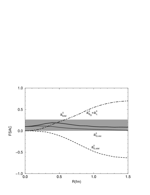
Our numerical results are given in Fig. 5.6. The quarkish component of the FSAC is given by the sum of the quark and $\eta$ contribution, $a^{0}_{B_{Q}}+a^{0}_{\eta}$ and the gluonic component by $a^{0}_{G,stat}+a^{0}_{G,vac}$. Both increase individually as the bag radius $R$ is increased but the sum remains small, $0<a^{0}_{total}<0.3$ for the whole range of radii.

Figure 5.7: The moment of inertia associated with the collective rotation as a function of the bag radius and the proton spin fraction carried by each constituents. In the calculation, we have used (a) the “confined” color electric field with $Q_{R}(r)$ and (b) the conventional one with $Q_{0}(r)$.

Refer to caption Refer to caption

Figure 5.8: The gluon spin $\Gamma$ as a function of the bag radius. (a) and (b) are obtained with the color electric fields explained in Fig. 5.7.

Refer to caption Refer to caption

Figure 5.9: The flavor singlet axial current $a_{0}$ as a function of the bag radius. (a) and (b) are obtained with the color electric fields explained in Fig. 5.7.

Refer to caption Refer to caption

Chapter 6 Discussion

This thesis deals with the description of hadronic phenomena from the perspective of QCD and low energy hadronic effective theories. The underlying goal has been the analysis of the realization of the Cheshire Cat principle in a realistic 3+1 dimensional scenario. We have reviewed in this thesis its formulation and have studied an extremely subtle case, namely the FSAC, an observable intimately related to the study of the spin of the proton, that lends support to the notion of the Cheshire Cat Principle in QCD governing strongly interacting systems. Before embarking onto the discussion of the results, let us stress that the consequences of quantum effects, through the chiral anomaly, the color anomaly and the Casimir phenomena have played a major role in the successful completion of this work.

In the previous chapter, we have considered various contributions to the FSAC of the proton. As presented in Fig. 5.2, the FSAC, which arises from the quarks, the $\eta^{\prime}$ meson and the (MIT or monopole) static gluons, fails to fulfill the Cheshire Cat Principle (CCP). For all cases the FSAC vanishes in the $R\rightarrow 0$ limit. The missing ingredient which is required to restore the principle is the Casimir effect that accounts for the fact that the modes are not free but strongly interacting via the boundary conditions of the cavity. The calculated Casimir contributions lead to a nonzero value of the FSAC even for zero bag radius.

Our numerical results are shown in Fig. 5.6. Standard MIT bag parameters were used for the calculation. The quarkish component of the FSAC is given by the sum of the quark and $\eta$ contributions, $a^{0}_{B_{Q}}+a^{0}_{\eta}$, and the gluonic component by $a^{0}_{G,stat}+a^{0}_{G,vac}$. Both contributions increase as the confinement size $R$ is increased but their sum remains small, $0<a^{0}_{total}<0.3$, for the whole range of radii, giving a value consistent with the experiment, $a^{exp}=a^{0}(\infty)=0.10^{+0.17}_{-0.10}$. It is remarkable that $a(R=0)\simeq a(R\approx 1.5\ {\rm fm})$, while each component can differ widely for the two extreme radii.

We have shown that the principal agent for the observed small FSAC in the proton, in the framework of the chiral bag model, is the CCP. It is the CCP that assures the cancellation between the different contributions: the quarkish and the gluonic. Note that the separation used by us is arbitrary and has no physical meaning, only the sum is physical.

For a small bag radius, both components are small, so the small net FSAC is inevitable. This is consistent with the observation that in the limit as $R\rightarrow 0$ we recover the skyrmion description, which gives vanishing FSAC at leading order, subject to small modification by matter fields at higher order. For a large bag radius – a limit that corresponds to the MIT bag model – both the quarkish and the gluonic contributions are separately large but they cancel each other. Our assertion is that this cancellation is mandated by the CCP. We should recall again that the separation between the quarkish component and the gluonic component adopted in eqs. (5.6) and (5.7) is entirely arbitrary although the sum is unique. Whether the different components by itself are large or small has no physical meaning. Only their sum does. Different separations would lead to different scenarios leading to the same small value. These different separations are analogs to gauge choices in gauge theories as suggested by some authors (see, e.g., [16]). It is tempting to speculate that in some limit, the FSAC is exactly zero and the the small nonzero value corresponds to a departure from this limit. Understanding this limit would allow a unique separation of the components.

One of the principal results of this thesis is that it is possible to have a nonzero value for the FSAC at $R=0$ and it is of the same size as that for large $R$. The reason for this nonzero value is intimately connected with the CCP, since it is the finite part of the gluon mode sum which normalizes the value of this contribution at the origin. Moreover, the color boundary condition provides us with a decreasing $\eta^{\prime}$ field contribution which changes softly as a function of $R$. While the effect of the surface color anomaly term is generally small for all radii, the finite nonzero value of the FSAC for $R=0$ is assured by the surface boundary term. Thus the violation of the CCP observed in the previous calculations at $R=0$ [22] [23] is neatly eliminated by the color anomaly boundary condition. More importantly, the monopole structure of the color electric field previously proposed is found to be required for the sign that comes with the important static gluonic contribution from the quark source. We believe that this cancellation is a manifestation in the bag scenario of the recently discovered one for $QCD$ [98]. The MIT configuration would strongly violate the CCP. We are thus led to the conclusion that the CCP requires the monopole configuration for the color electric field. Whether or not this configuration leaves undisturbed other – successful – phenomenology was discussed in [22].

In calculating the gluonic Casimir effect, we made the ab initio assumption that the CCP holds, an assumption which is expected to be valid for small bag radius. We then extended it, in accordance with the CCP, to all bag radii. We can justify this only à posteriori by showing that the CCP assumption is consistent with what one obtains. Note, however, that the gluonic Casimir effect is most significant for small $R$ where it is needed for the CCP and plays little role for large $R$. Thus our assumption is validated. It would of course be more satisfying if one could obtain the CCP as an output of the formalism, not put in as an input. To this end, we need to solve appropriate equations of motion for gluons to the color boundary conditions (4.70). Since the color anomaly boundary conditions are generated by the quantum effect of quark, it is necessary to consider an effective action for gluons which contains the quantum effect resulting from integrating out quark fields. Although gluons have been treated as abelianized (or Maxwell) fields in the previous chapter, we should give special care in the abelianization because of the nontrivial topological structure of the QCD [99]. Therefore, we need to construct an effective action for the bagged QCD and see there are additional corrections besides the Maxwell terms in the effective action.

We should mention a caveat left unspecified in Chapter 5 in regularizing this Casimir contribution. Since $a_{G,vac}^{0}$ vanishes when $\eta^{\prime}$ field is removed, the so-called “vacuum contribution” is duly subtracted in what we have computed. However, we have also explicitly subtracted quadratic and linear divergences appearing from the mode sum by resorting to a procedure used in most of Casimir-type calculation [100], which, as far as we know, is physically reasonable but has not yet been rigorously justified from the first principles 111It is found that the specific structure of the divergent terms depends on regularization schemes whereas that of the finite terms does not [94].. The same caveat applies to our calculation as it does to others. The finite term we have obtained might therefore be subject to additional finite corrections by procedures in the renormalization.

We should also stress that our result is at best qualitative. A better treatment (such as a more realistic gauge coupling constant running with the bag size, a more accurate calculation of $A^{vac}_{G}$, etc…) might modify our results quantitatively. Even so, we believe it to be quite robust that the overall FSAC is small, $\stackrel{{\scriptstyle<}}{{\sim}}0.3$ and that it is more or less independent of the confinement size.

Bibliography

  • [1]
  • [2] M. Gell-Mann and Y. Ne’eman, “The eightfold way,” (Benjamin, New York, 1964); G. Zweig, CERN Report no. 8182/TH 401.
  • [3] R. P. Feynman, “Photon-Hadron Interaction,” (W. A. Benjamin, New York, 1972).
  • [4] J. J. J. Kokkedee, “The Quark Model,” (W. A. Benjamin, New York 1969); D. B. Lichtenberg, “Unitary Symmetry and Elementary Particles,” (Academic Press, Inc. New York 1978).
  • [5] S. Okubo, Phys. Lett. 5 (1963) 163; G. Zweig, CERN Report no. 8419/TH 412; J. Iizuka, Prog. Theor. Phys. Suppl. 37-38 (1966) 21.
  • [6] T. Muta, “Foundations of Quantum ChromoDynamics,” (World Scientific, Singapore 1987); R. D. Field “Applications of perturbative $QCD$,” (Addison Wesley Pub. Co. 1989); F.J. Yndurain. “The Theory of the Quark and Gluon Interactions,” (Springer Verlag 1999
  • [7] F. E. Close, “An introduction to quarks and partons,” (Academic Press, London, 1979); R.F. Alvarez-Estrada, F. Fernández, J.L. Sánchez Gómez and V. Vento, “Model of Hadron Structure based on QCD,” Lecture Notes in Physics 259 (Springer Verlag Heidelberg 1986).
  • [8] A. de Rújula, H. Georgi and S.L. Glashow, Phys. Rev. D12 (1975) 147.
  • [9] N. Isgur and G. Karl, Phys. Lett. 72B (1977) 109; Phys. Lett. 74B (1978) 353; Phys. Rev. D 18 (1978) 4187; Phys. Rev. D 20 (1979) 1191.
  • [10] A. Chodos, R. L. Jaffe, K. Johnson, C. B. Thorn and V. Wesskopf, Phys. Rev. D9 (1974) 3471; A. Chodos, R. L. Jaffe, K. Johnson and C. B. Thorn, Phys. Rev. D10 (1974) 2559; T. DeGrand, R. L. Jaffe, K. Johnson and J. Kiskis, Phys. Rev. D12 (1975) 2060; P. Hasenfratz and J. Kuti, Phys. Rep. 40 (1978) 75.
  • [11] A. Chodos and C. B. Thorn, Phys. Rev. D12 (1975) 2733.
  • [12] G. E. Brown and M. Rho, Phys. Lett. 82B (1979) 177; G. E. Brown, M. Rho and V. Vento, Phys. Lett. 94B (1979) 383.
  • [13] T. H. R. Skyrme, Proc. R. Soc. London A260 (1961) 127; A262 (1961) 237.
  • [14] E. Witten, Nucl. Phys. B223 (1983) 422; Nucl. Phys. B223 (1983) 433.
  • [15] H.B. Nielsen and A. Wirzba, “Elementary Structure of Matter,” Springer Proceedings in Physics 26 (1988); Proc. on the fundamental structure of hadronic matter, Les Houches France (1987); S. Nadkarni, H.B. Nielsen and I. Zahed, Nucl. Phys. B253 (1985) 308; S. Nadkarni and H.B. Nielsen, Nucl. Phys. B263 (1986) 1; S.Nadkarni and I. Zahed, Nucl. Phys. B263 (1986) 23; R. Perry and M. Rho, Phys. Rev. D34 (1986) 1169.
  • [16] For detailed review, see, e.g., “Chiral Nuclear Dynamics,” by M.A. Nowak, M. Rho and I. Zahed (World Scientific Pub. Singapore, 1996) Chapter 8.
  • [17] S. Coleman, Phys. Rev. D11 (1975) 2088; S. Mandelstam, Phys. Rev. D11 (1975) 3026; A. Ferrando and V. Vento, Phys. Rev. D49 (1994) 3044.
  • [18] S. Weinberg, Physica 96A (1979) 327; “The Quantum Theory of Fields II,” (Cambridge Press, 1996); Nature 386 (1997) 234; H. Georgi, “Weak Interactions and Modern Particle Physics,” (The Benjamin/Cummings Pub. Co., Menlo Park, CA, 1984).
  • [19] T. H. R. Skyrme, Nucl. Phys. 31 (1962) 556; J. Gasser and H. Leutwyler, Ann. Phys. 158 (1984) 142.
  • [20] V. Vento, M. Rho, E.M. Nyman, J.H. Jun and G.E. Brown, Nucl. Phys. A345 (1980) 413; G.E. Brown, A.D. Jackson, M. Rho and V. Vento, Phys. Lett. B140 (1984) 285.
  • [21] B.-Y. Park, V. Vento, M. Rho and G. E. Brown, Nucl. Phys. A504 (1989) 829.
  • [22] B.-Y. Park and V. Vento, Nucl. Phys. A513 (1990) 413.
  • [23] M. Rho and V. Vento, Nucl. Phys. A662 (1997) 538.
  • [24] M. J. Alguard et al., Phys. Rev. Lett. 41 (1978) 70.
  • [25] G. Baum et al., Phys. Rev. Lett. 51 (1983) 1135.
  • [26] J. Ashman et al., Phys. Lett. B206 (1988) 364; Nucl. Phys. B328 (1989) 1.
  • [27] J. Ellis and R. L. Jaffe, Phys. Rev. D9 (1974) 1444; Phys. Rev. D10 (1974) 1669.
  • [28] A. V. Efremov and O. V. Terytaev, JINR Report E2-88-287 (1988); G. Altarelli and G. G. Ross, Phys. Lett. B212 (1988) 391; R. D. Carlitz, J. C. Collins and A. H. Mueller, Phys. Lett. B214 (1988) 229; R. D. Ball, “Perturbative Evolution of Polarized Structure Functions,” Erice 1995, Eds. B. Frois, V.W. Hughes and N. de Groot (World Scientific, Singapore 1997).
  • [29] A. Adler and W. A. Bardeen, Phys. Rev. 182 (1969) 1517; J. S. Bell and R. Jakiw, Nuovo. Cim. A51 (1967) 47; S. B. Treiman, R. W. Jackiw, B. Zumino, and E. Witten, in “Current algebra and anomalies,” (World Scientific, Singapore, 1996).
  • [30] G. ’t Hooft, Phys. Rep. 142 (1986) 357.
  • [31] M. Rho, A.S. Goldhaber, G.E. Brown, Phys. Rev. Lett. 51 (1983) 747; J. Goldstone and R.L. Jaffe, Phys. Rev. Lett. 51 (1983) 1518; G.E. Brown, A.D. Jackson, M. Rho and V. Vento, Phys. Lett. B140 (1984) 285; A.D. Jackson, L. Vepstas, E. Wüst and D. Kahana, Nucl. Phys. A462 (1987) 661.
  • [32] B.-Y. Park and M. Rho, Z. Phys. A331 (1988) 151.
  • [33] B.-Y. Park, Z. Phys. A331 (1988) 473.
  • [34] H. B. Nielsen, M. Rho, A. Wirzba and I. Zahed, Phys. Lett. B269 (1991) 389.
  • [35] M. Anselmino, A. Efremov, and E. Leader, Phys. Rep. 261 (1995) 1.
  • [36] S. D. Drell and j. D. Wallecka, Ann. Phys. 28 (1964) 18; J. D. Bjorken, Phys. Rev. 148 (1966) 1467;C. E. Carlson and Wu-ki Tung, Phys. Rev. D5 (1972) 721; A. J. G. Hey and J. E. Madular, Phys. Rev. D5 (1972) 2610.
  • [37] A. V. Manohar, “An introduction to spin dependent deep inelastic scattering,” hep-ph/9204208.
  • [38] J. D. Bjorken, Phys. Rev. 179 (1969) 1547.
  • [39] H.-Y. Cheng, Int. J. Mod. Phys. A11 (1996) 5109.
  • [40] M. J. Alguad et al, Phys. Rev. Lett. 37 (1976) 1261; Phys. Rev. Lett. 41 (1978) 70; G. Baum et al, Phys. Rev. Lett. 45 (1980) 2000.
  • [41] G. Baum et al, Phys. Rev. Lett. 51 (1983) 1135.
  • [42] B. Adeva et al, Phys. Lett. B302 (1993) 533.
  • [43] B. Adams et al, Phys. Lett. B329 (1994) 399; B339 (1994) 332(E).
  • [44] B. Adams et al, Phys. Lett. B357 (1995) 248.
  • [45] P. L. Anthony et al, Phys. Rev. Lett. 71 (1993) 959.
  • [46] K. Abe et al, Phys. Rev. Lett. 75 (1995) 25.
  • [47] K. Abe et al, Phys. Rev. Lett. 74 (1995) 346.
  • [48] T. -P. Cheng and L.-F. Li, “Gauge theory of elementary particle physics,” (Oxford University Press, New York, 1985).
  • [49] G. M. Shore, Nucl. Phys. B (Proc. Suppl.) 64 (1998) 167.
  • [50] S. A. Larin and J. A. M. Vermaseren, Phys. Lett. B259 (1991) 345; S. A. Larin, Phys. Lett. B334 (1994) 192.
  • [51] Paticle Data Group, Eur. J. Phys, C3 (1998) 1.
  • [52] Y. Goto et al, Phys.Rev. D62 (2000) 034017.
  • [53] L. M. Sehgal, Phys. Rev. D10 (1974) 1663.
  • [54] J. Schechter and H. Weigel, “The Skyrme Model for Baryons,” hep-ph/9907554.
  • [55] H. -Y. Cheng, “The proton spin puzzle: A status report,” hep-ph/0002157.
  • [56] R. L. Jaffe, Phys. Lett. B365 (1996) 359.
  • [57] For disccusion, see G. E. Brown and M. Rho, Comments part. Nucl. Phys. 18 (1988)1; A. Chodos and C. B. Thorn, Phys. Rev. D12 (1975) 2733.
  • [58] D. J. Gross, in ”Methods in field theory”, R. Balian and J. Zinn-Justin, eds. (North Holland, Amsterdam, 1976).
  • [59] T. Hatsuda and I. Zahed, Phys. Lett. B221 (1989) 173.
  • [60] J. Wess and B. Zumino, Phys. Lett. B37(1971) 95; E. Witten, Nucl. Phys. B223 (1983) 422.
  • [61] M. A. Nowak, P. O. Mazur and M. Praszalowicz, Phys. Lett. B147 (1984) 137; E. Guadagnini, Nucl. Phys. B236 (1985) 35.
  • [62] G. E. Brown, A. D. Jackson, M. Rho and V. Vento, Phys. Lett. B140 (1984) 285; M. Rho, A. S. Goldhaber and G. E. Brown, Phys. Rev. Lett. bf 51 (1983) 747.
  • [63] J. Goldstone and R. L. Jaffe, Phys. Rev. Lett. 51 (1983) 1518.
  • [64] A. Hosaka and H. Toki, Phys. Rep. 277 (1996) 65.
  • [65] R. J. Perry and M. Rho, Phys. Rev. D34 (1986) 1169.
  • [66] V. Vento, “The Cheshire Cat revisited” in Proceedings of the APCTP Workshop on Astro-Hadron Physics (World Scientific, Singapore, 1999).
  • [67] I. Zahed and G. E. Brown, Phys. Rep. 142 (1986) 1169; G. S. Adkins, in “Chiral Solitons,” ed. K. F. Liu (World Scientific, Singapre, 1987).
  • [68] D. Inglis, Phys. Rev. 96 (1954) 1059; D. J. Thouless and J. G. Valatin, Nucl. Phys. 31 (1962) 211.
  • [69] M. Praszalowicz, Phys. Lett. B158 (1985) 264; M. Chemtob, Nucl. Phys. B256 (1985) 600.
  • [70] T. D. Lee, “Particle physics and introduction to field theory,” (Harwood academic publishers, 1981).
  • [71] A. Maxwell and V. Vento, Nucl. Phys. A407 (1983) 882.
  • [72] T. D. Lee, Phys. Rev. D19 (1979) 1802.
  • [73] J. Wroldsen and F. Myhrer, Z. Phys. C25 (1984) 59.
  • [74] C. Itzyson and J. -B. Zuber, “Quantum field theory,” (McGraw-Hill, New York, 1980).
  • [75] T.-P. Cheng and L.-F. Li, “Gauge theory of elementary particle physics,” (Clarendon Press, Oxford, 1988): R. A. Bertlmann, “Anomalies in Quantum Field Theory,” (Clarendon Press, Oxford, 1996).
  • [76] A. Adler and W. A. Bardeen, Phys. Rev. 182 (1969) 1517.
  • [77] M. A. Shifman, Phys. Rep. 209 (1991) 341
  • [78] P. Ramond, “Field theory: A modern primer,” (Addison-Wesley Publishing Company, 1990).
  • [79] R. Jakiw, “Current algebra and anomalies,” (World scientific, Singapore, 1985).
  • [80] G. ’t Hoot, Phys. Rev. Lett. 37 (1976) 8; G. ’t Hoot, Phys. Rev. D29 (1976) 3432; C. Callan, R. Dashen, and D. Gross, Phys. Lett. B63 (1976) 334.
  • [81] T. H. Hansson and R. L. Jaffe, Phys. Rev. D28 (1983) 882.
  • [82] J. Schwinger, Phys. Rev. 82 (1951) 664; S. K. Blau, M. Visser and A. Wipf, Nucl. Phys. B 310 (1988) 16; I. J. R. Aitchison, C. M. Fraser, Phys. Rev. D 31 (1985) 2605.
  • [83] H. B. Nielsen, M. Rho, A. Wirzba, and I. Zahed, Phys. Lett. B281 (1992) 345.
  • [84] M.A. Shifman, in “Vacuum structure and QCD sum rules,” (North Holland, Amsterdam 1992); S. Narison, in “QCD spectral sum rules,” (World Scientific, Singapore 1989).
  • [85] H.-J. Lee, D.-P. Min, B.-Y. Park, M. Rho, and V. Vento, Phys. Lett. B491 (2000) 257.
  • [86] L. Mankiewicz, G. Piller and A. Saalfeld, Phys. Lett. B395 (1997) 318.
  • [87] V. Barone, T. Calarco and A. Drago, Phys. Lett. B431 (1998) 405.
  • [88] R. L. Jaffe and A. Manohar, Nucl. Phys. B337 (1990) 509.
  • [89] H.-J. Lee, D.-P. Min, B.-Y. Park, M. Rho and V. Vento, Nucl. Phys. A657 75.
  • [90] P.H. Damgaard, H.B. Nielsen and R. Sollacher, Nucl. Phys. B385 (1992) 227; Phys. Lett. B298 (1992) 132.
  • [91] H. B. G. Casimir, Proc. Kon. Ned. Akad. Wet. 51 (1948) 793.
  • [92] G. Plunien, B. Muller, and W. Greiner, Phys. Rep. 134 (1986) 87.
  • [93] S. Weinberg, “Quantum theory of fields II,” (Cambridge Univ. Press, New York, 1996).
  • [94] F. Ravndal, “Problems with the Casimir vacuum energy,” hep-ph/0009208.
  • [95] K. A. Milton, Ann. Phys. 115 (1978) 388; K. A. Milton, Phys. Rev. D22 (1980) 1441; 1444; D27 (1983) 439; I. Zahed et al, Ann. Phys. 165 (1985) 406; M. de Francia, Phys. Rev. D50 (1994) 2908; V. V. Nesterenko, Phys. Rev. D57 (1998) 1284.
  • [96] S. Forte, Proceedings of PANIC96, Williamsburg, May 1996 and SPIN96, Amsterdam, September 1996, hep-ph/9601238.
  • [97] V. A. Novikov, M.A. Shifman, A.I. Vainstein and V.I. Zakharov, Nucl. Phys. B 191 (1981) 301.
  • [98] N. Kochelev and V. Vento, hep-ph/9809238.
  • [99] Y. M. Cho, Phys. Rev. D21 (1980) 1080; Y. M. Cho, H. Lee, and D. G. Pak, hep-th/0104058.
  • [100] J. Schwinger, Lett. Math. Phys. 24 (1992) 59, 227; Proc. Natl. Acad. Sci. USA 89 (1992) 4091, 11118; K. A. Milton and Y. Jack Ng, Phys. Rev. E57 (1998) 5504.
  • [101] A. R. Edmonds, “Angular momentum in the quantum mechanics,” (Princeton Univ. press, 1957).
  • [102] G. B. Arfken and H. J. Weber, “Mathematical methods for physicists,” (Academic press, 1995).
  • [103] We thank Dr. Klaus Kirsten for providing us with this proof.
  • [104] G.N. Watson, “Theory of Bessel Functions,” (Cambridge University press, Cambridge, 1944).
  • [105] I.S. Gradshteyn and I.M. Ryzhik, “Table of Integrals, Series and Products,” (Academic Press, New York, 1965).

Appendix A Angular momentum basis of the wave functions for the strange and the hedgehog quarks

In this appendix, we present explicit expressions of the angular momentum basis for the strange quark (s-quark) wave functions, $|j,m_{j}\rangle_{\kappa}$, which are eigenstates of ${\bf J}^{2}$ and $J_{z}$, and those for the hedgehog quark (h-quark) wave functions, $|K,m_{K}\rangle_{i}$, which are eigenstates of ${\bf K}^{2}$ and $K_{z}$. Here $\kappa=\pm 1$ and $i$ runs over $1,2,3,4.$

The basis $|j,m_{j}\rangle_{\kappa}$ can be constructed by combining the orbital angular momentum basis $|l,m_{j}\rangle$ and the spin basis $|\frac{1}{2},m_{s}\rangle_{s}$, which are eigenstates of the orbital angular momentum operators ${\bf L}^{2}$ and $L_{z}$ and the spin operators ${\bf S}^{2}$ and $S_{z}$, respectively. According to the angular momentum sum rule, there are two types.

i) $j=l+\frac{1}{2}$ and $\kappa=1$:

$\displaystyle|j,m_{j}\rangle_{1}$ $\displaystyle=$ $\displaystyle\bigg{(}\frac{j+m_{j}}{2j}\bigg{)}^{\frac{1}{2}}|j,m_{j}-1/2\rangle|1/2,1/2\rangle_{s}$ (A.1)
$\displaystyle+\bigg{(}\frac{j-m_{j}}{2j}\bigg{)}^{\frac{1}{2}}|j,m_{j}-1/2\rangle|1/2,-1/2\rangle_{s},$

ii) $j=l-\frac{1}{2}$ and $\kappa=-1$:

$\displaystyle|j,m_{j}\rangle_{-1}$ $\displaystyle=$ $\displaystyle-\bigg{(}\frac{j-m_{j}+1}{2j+2}\bigg{)}^{\frac{1}{2}}|j,m_{j}-1/2\rangle|1/2,1/2\rangle_{s}$ (A.2)
$\displaystyle+\bigg{(}\frac{j+m_{j}+1}{2j+2}\bigg{)}^{\frac{1}{2}}|j,m_{j}-1/2\rangle|1/2,-1/2\rangle_{s}.$

The conventions of Edmonds [101] for the Clebsch-Gordan coefficients have been used. One can see that these two type of solutions have opposite parity for a given $j$.

Using the following identities [102],

$\displaystyle\cos\theta\ Y_{l}^{m}=\bigg{[}\frac{l-m+1}{2l+1}\cdot\frac{l+m+1}{2l+3}\bigg{]}^{\frac{1}{2}}Y_{l+1}^{m}+\bigg{[}\frac{l-m}{2l-1}\cdot\frac{l+m}{2l+1}\bigg{]}^{\frac{1}{2}}Y_{l-1}^{m},$ (A.3)
$\displaystyle\sin\theta\ e^{i\phi}Y_{l}^{m}=-\bigg{[}\frac{l+m+1}{2l+1}\cdot\frac{l+m+2}{2l+3}\bigg{]}^{\frac{1}{2}}Y_{l+1}^{m+1}+\bigg{[}\frac{l-m}{2l-1}\cdot\frac{l-m-1}{2l+1}\bigg{]}^{\frac{1}{2}}Y_{l-1}^{m+1}$
$\displaystyle\sin\theta\ e^{-i\phi}Y_{l}^{m}=\bigg{[}\frac{l-m+1}{2l+1}\cdot\frac{l-m+2}{2l+3}\bigg{]}^{\frac{1}{2}}Y_{l+1}^{m-1}+\bigg{[}\frac{l+m}{2l-1}\cdot\frac{l+m-1}{2l+1}\bigg{]}^{\frac{1}{2}}Y_{l-1}^{m-1},$

where $Y_{l}^{m}$ is the spherical harmonics, one can show that the above states satisfy,

$$\mbox{\boldmath$\sigma$}\cdot\hat{\bf r}\ |j,m_{j}\rangle_{\pm}=-|j,m_{j}\rangle_{\mp}.$$ (A.4)

The basis for the hedgehog quark, $|K,m_{K}\rangle_{i}$, can be obtained by combining the total angular momentum ${\bf J}$ and the isospin ${\bf I}$. In this case there are four types of states given by,

i) ${\rm i}=1\;\bigg{(}j=l+\frac{1}{2},\ K=j-\frac{1}{2}\bigg{)},$

$\displaystyle|K,m_{K}\rangle_{1}$ $\displaystyle=$ $\displaystyle-\bigg{(}\frac{K-m_{K}+1}{2K+2}\bigg{)}^{\frac{1}{2}}|j,m_{K}-1/2\rangle_{1}|1/2,+1/2\rangle_{t}$ (A.5)
$\displaystyle+\bigg{(}\frac{K+m_{K}+1}{2K+2}\bigg{)}^{\frac{1}{2}}|j,m_{K}+1/2\rangle_{1}|1/2,-1/2\rangle_{t},$

ii) ${\rm i}=2\;\bigg{(}j=l-\frac{1}{2},\ K=j+\frac{1}{2}\bigg{)},$

$\displaystyle|K,m_{K}\rangle_{2}$ $\displaystyle=$ $\displaystyle\bigg{(}\frac{K+m_{K}}{2K}\bigg{)}^{\frac{1}{2}}|j,m_{K}-1/2\rangle_{-1}|1/2,+1/2\rangle_{t}$ (A.6)
$\displaystyle+\bigg{(}\frac{K-m_{K}}{2K}\bigg{)}^{\frac{1}{2}}|j,m_{K}+1/2\rangle_{-1}|1/2,-1/2\rangle_{t},$

iii) ${\rm i}=3\;\bigg{(}j=l-\frac{1}{2},\ K=j-\frac{1}{2}\bigg{)},$

$\displaystyle|K,m_{K}\rangle_{3}$ $\displaystyle=$ $\displaystyle-\bigg{(}\frac{K-m_{K}+1}{2K+2}\bigg{)}^{\frac{1}{2}}|j,m_{K}-1/2\rangle_{-1}|1/2,+1/2\rangle_{t}$ (A.7)
$\displaystyle+\bigg{(}\frac{K+m_{K}+1}{2K+2}\bigg{)}^{\frac{1}{2}}|j,m_{K}+1/2\rangle_{-1}|1/2,-1/2\rangle_{t},$

iv) ${\rm i}=4\;\bigg{(}j=l+\frac{1}{2},\ K=j-\frac{1}{2}\bigg{)},$

$\displaystyle|K,m_{K}\rangle_{4}$ $\displaystyle=$ $\displaystyle\bigg{(}\frac{K+m_{K}}{2K}\bigg{)}^{\frac{1}{2}}|j,m_{K}-1/2\rangle_{1}|1/2,+1/2\rangle_{t}$ (A.8)
$\displaystyle+\bigg{(}\frac{K-m_{K}}{2K}\bigg{)}^{\frac{1}{2}}|j,m_{K}+1/2\rangle_{1}|1/2,-1/2\rangle_{t},$

where the subscript $t$ has been used to label states in the isospace.

Since $K=l$ for $i=1,2$ and $K=l-1$ for $i=3,4$, one can check that $|K,m_{K}\rangle_{1}$ and $|K,m_{K}\rangle_{2}$ have parity $(-1)^{K}$, whereas $|K,m_{K}\rangle_{3}$ and $|K,m_{K}\rangle_{4}$ have parity $-(-1)^{K}$.

Using the identity eq. (A), one can show that the states $|K,m_{K}\rangle_{i}$ satisfy the relation

$$\mbox{\boldmath$\sigma$}\cdot\hat{\bf r}\ |K,m_{K}\rangle_{i}=-|K,m_{K}\rangle_{i+2}.$$ (A.9)

Besides, applying the operator $\mbox{\boldmath$\tau$}\cdot\hat{\bf r}$ to $|K,m_{K}\rangle_{i}$ where $\tau$ are the Pauli matrices in isospace, we have the following relations;

$\displaystyle\mbox{\boldmath$\tau$}\cdot\hat{\bf r}\ |K,m_{K}\rangle_{1}=\frac{2j-2K}{2K+1}\ |K,m_{K}\rangle_{3}-2\frac{\sqrt{K(K+1)}}{2K+1}\ |K,m_{K}\rangle_{4},$ (A.10)
$\displaystyle\mbox{\boldmath$\tau$}\cdot\hat{\bf r}\ |K,m_{K}\rangle_{2}=\frac{2j-2K}{2K+1}\ |K,m_{K}\rangle_{4}-2\frac{\sqrt{K(K+1)}}{2K+1}\ |K,m_{K}\rangle_{3},$ (A.11)
$\displaystyle\mbox{\boldmath$\tau$}\cdot\hat{\bf r}\ |K,m_{K}\rangle_{3}=\frac{2j-2K}{2K+1}\ |K,m_{K}\rangle_{1}-2\frac{\sqrt{K(K+1)}}{2K+1}\ |K,m_{K}\rangle_{2},$ (A.12)
$\displaystyle\mbox{\boldmath$\tau$}\cdot\hat{\bf r}\ |K,m_{K}\rangle_{4}=\frac{2j-2K}{2K+1}\ |K,m_{K}\rangle_{2}-2\frac{\sqrt{K(K+1)}}{2K+1}\ |K,m_{K}\rangle_{1},$ (A.13)

where we have used the fact that $K$ in $|K,m_{K}\rangle_{1,3}$ is $j-{1\over 2}$ and $K$ in $|K,m_{K}\rangle_{2,4}$ is $j+\frac{1}{2}$. These relations have been used to get the energy levels for the hedgehog quarks.

Appendix B Proof that the sum over E-modes is zero

We have shown that the contribution of E-modes to the Casimir effect of the FSAC vanishes numerically in Chapter 5. In this appendix, we show an analytical proof of this result [103]. Let’s consider $I(x)$ given in Chapter 5;

$\displaystyle I(x)=\int_{0}^{x}dy\,\,y^{3}\left[j_{J}^{2}(y)-\frac{J}{2J+1}j_{J+1}^{2}(y)-\frac{J+1}{2J+1}j_{J-1}^{2}(y)\right],$

and the boundary condition for the E-modes

$$j_{J}(X_{n})=0,$$ (B.1)

where $X_{n}=\omega_{n}R$. To prove $I(X_{n})=0$, it is convenient to use formulae of the Bessel functions rather than the spherical Bessel functions. From the definition

$\displaystyle j_{l}(x)=\sqrt{\frac{\pi}{2x}}J_{l+1/2}(x),$

we can rewrite $I(x)$ in terms of the Bessel functions

$\displaystyle I(x)=\frac{\pi}{2}\int_{0}^{x}dy\,\,y^{2}\left[J^{2}_{J+1/2}(y)-\frac{J}{2J+1}J^{2}_{J+3/2}(y)-\frac{J+1}{2J+1}J^{2}_{J-1/2}(y)\right],$ (B.2)

and the boundary condition

$\displaystyle J_{J+1/2}(X_{n})=0.$ (B.3)

Using the following formula by Schafheitlin [104];

$\displaystyle(\mu+2)\int_{0}^{z}dx\,\,x^{\mu+2}J_{\nu}^{2}(x)=(\mu+1)\left(\nu^{2}-\frac{(\mu+1)^{2}}{4}\right)\int_{0}^{z}dx\,\,x^{\mu}J_{\nu}^{2}(x)$
$\displaystyle+\frac{1}{2}\left[z^{\mu+1}\left(zJ_{\nu}^{\prime}(z)-\frac{1}{2}(\mu+1)J_{\nu}(z)\right)^{2}+z^{\mu+1}\left(z^{2}-\nu^{2}+\frac{1}{4}(\mu+1)^{2}\right)J_{\nu}^{2}(z)\right].$

we can arrange $I(x)$ in terms of Bessel functions, its derivatives and simpler integrals with a lower power in $y$.

In the next step, we use the recursion relations of the Bessel functions in order to write $I(x)$ in terms of the Bessel functions with an index $J+\frac{1}{2}$. In addition, to get more useful expressions, we decompose $I(x)$ into the three terms

$\displaystyle I_{1}(x)$ $\displaystyle=$ $\displaystyle\frac{\pi}{2}\int_{0}^{x}dy\,\,y^{2}J_{J+1/2}^{2}(y)$ (B.5)
$\displaystyle I_{2}(x)$ $\displaystyle=$ $\displaystyle-\frac{\pi}{2}\frac{J}{2J+1}\int_{0}^{x}dy\,\,y^{2}J_{J+3/2}^{2}(y)$ (B.6)
$\displaystyle I_{3}(x)$ $\displaystyle=$ $\displaystyle-\frac{\pi}{2}\frac{J+1}{2J+1}\int_{0}^{x}dy\,\,y^{2}J_{J-1/2}^{2}(y).$ (B.7)

Using Schafheitlin’s formula (B) and eq. (B.3), we have immediately

$\displaystyle I_{1}(X_{n})=\frac{\pi}{4}\left\{\frac{1}{2}X_{n}^{3}J_{J+1/2}^{\prime 2}(X_{n})+J(J+1)\int_{0}^{X_{n}}dy\,\,J_{J+1/2}^{2}(y)\right\}$ (B.8)

The second expression has a more complicated form in terms of Bessel functions, i.e.

$\displaystyle I_{2}(X_{n})$ $\displaystyle=$ $\displaystyle-\frac{\pi}{4}\frac{J}{2J+1}\left\{\right.[J^{2}+3J+2]\int_{0}^{X_{n}}dy\,\,J_{J+3/2}^{2}(y)$
$\displaystyle+\frac{1}{2}X_{n}^{3}J_{J+3/2}^{\prime 2}(X_{n})-\frac{1}{2}X_{n}^{2}J_{J+3/2}^{\prime}(X_{n})J_{J+3/2}(X_{n})$
$\displaystyle\left.+\frac{1}{2}X_{n}\left[X_{n}^{2}-J^{2}-3J-\frac{7}{4}\right]J_{J+3/2}^{2}(X_{n})\right\}.$

From the recursion relation of the Bessel functions [105], one gets

$\displaystyle J_{J+3/2}(y)=-J^{\prime}_{J+1/2}(y)+\frac{J+1/2}{y}J_{J+1/2}(y),$

which yields by the boundary condition eq. (B.3)

$\displaystyle J_{J+3/2}(X_{n})=-J^{\prime}_{J+1/2}(X_{n}).$

Similarly

$\displaystyle J_{J+3/2}^{\prime}(y)=-\frac{J+3/2}{y}J_{J+3/2}(y)+J_{J+1/2}(y),$

which means

$\displaystyle J_{J+3/2}^{\prime}(X_{n})=\frac{J+3/2}{X_{n}}J_{J+1/2}^{\prime}(X_{n})$

So finally the following form for $I_{2}(X_{n})$ is obtained,

$\displaystyle I_{2}(X_{n})=-\frac{\pi}{4}\frac{J}{2J+1}\left\{J_{J+1/2}^{\prime 2}(X_{n})\left[\frac{1}{2}X_{n}^{3}+\frac{1}{2}X_{n}J+X_{n}\right]\right.$
$\displaystyle+[J^{2}+3J+2]\int_{0}^{X_{n}}dy\,\,\left[J_{J+1/2}^{\prime 2}(y)-\frac{2J+1}{y}J_{J+1/2}(y)J_{J+1/2}^{\prime}(y)\right.$
$\displaystyle\left.\left.\hskip 113.81102pt+\frac{(J+1/2)^{2}}{y^{2}}J_{J+1/2}^{2}(y)\right]\right\}.$

For $I_{3}$ an intermediate result after applying Schafheitlin’s reduction formula (B.3) reads,

$\displaystyle I_{3}(X_{n})$ $\displaystyle=$ $\displaystyle-\frac{\pi}{4}\frac{J+1}{2J+1}\left\{[J^{2}-J]\int_{0}^{X_{n}}dy\,\,J_{J-1/2}^{2}(y)\right.$
$\displaystyle+\frac{1}{2}X_{n}^{3}J_{J-1/2}^{\prime 2}(X_{n})-\frac{1}{2}X_{n}^{2}J_{J-1/2}^{\prime}(X_{n})J_{J-1/2}(X_{n})+\frac{1}{8}X_{n}J_{J-1/2}^{2}(X_{n})$
$\displaystyle\left.+\frac{1}{2}X_{n}(X_{n}^{2}-J^{2}+J)J_{J-1/2}^{2}(X_{n})\right\}.$

Using this time

$\displaystyle J_{J-1/2}(X_{n})$ $\displaystyle=$ $\displaystyle J_{J+1/2}^{\prime}(X_{n})$
$\displaystyle J_{J-1/2}^{\prime}(X_{n})$ $\displaystyle=$ $\displaystyle\frac{J-1/2}{X_{n}}J_{J+1/2}^{\prime}(X_{n})$

it can be rewritten in the form

$\displaystyle I_{3}(X_{n})$ $\displaystyle=$ $\displaystyle-\frac{\pi}{4}\frac{J+1}{2J+1}\left\{{J_{J+1/2}^{\prime}}^{2}(X_{n})\left[\frac{1}{2}X_{n}^{3}-\frac{1}{2}X_{n}J+\frac{1}{2}X_{n}\right]\right.$
$\displaystyle+[J^{2}-J]\int_{0}^{X_{n}}dy\,\,\left[J_{J+1/2}^{\prime 2}(y)+\frac{2J+1}{y}J_{J+1/2}^{\prime}(y)J_{J+1/2}(y)\right.$
$\displaystyle\left.\left.\hskip 113.81102pt+\frac{(J+1/2)^{2}}{y^{2}}J_{J+1/2}^{2}(y)\right]\right\}.$

Before actually adding up all three pieces, it is better to have a further consideration. The integrals involve three different types of terms, namely $J_{J+1/2}^{\prime 2}$, $J_{J+1/2}J_{J+1/2}^{\prime}$ and $J_{J+1/2}^{2}$. However, these are not independent from each other due to the differential equation they fulfill. The differential equation for the Bessel functions reads

$\displaystyle\frac{d^{2}J_{J+1/2}(y)}{dy^{2}}+\frac{1}{y}\frac{dJ_{J+1/2}(y)}{dy}+\left(1-\frac{(J+1/2)^{2}}{y^{2}}\right)J_{J+1/2}(y)=0,$

and therefore we have

$\displaystyle\int_{0}^{X_{n}}dy\,\,J_{J+1/2}^{\prime 2}(y)$ $\displaystyle=$ $\displaystyle-\int_{0}^{X_{n}}dy\,\,J_{J+1/2}(y)\frac{d^{2}}{dy^{2}}J_{J+1/2}(y)$
$\displaystyle=$ $\displaystyle\int_{0}^{X_{n}}\left\{\frac{1}{y}J_{J+1/2}(y)J_{J+1/2}^{\prime}(y)+\left[1-\frac{(J+1/2)^{2}}{y^{2}}\right]J_{J+1/2}^{2}(y)\right\}.$

Using this identity, $I_{2}(X_{n}),I_{3}(X_{n})$ simplify to,

$\displaystyle I_{2}(X_{n})$ $\displaystyle=$ $\displaystyle-\frac{\pi}{4}\frac{J}{2J+1}\left\{J_{J+1/2}^{\prime 2}(X_{n})\left[\frac{1}{2}X_{n}^{3}+\frac{1}{2}X_{n}J+X_{n}\right]\right.$
$\displaystyle\left.+[J^{2}+3J+2]\int_{0}^{X_{n}}dy\left[J_{J+1/2}^{2}(y)-\frac{2J}{y}J_{J+1/2}(y)J_{J+1/2}^{\prime}(y)\right]\right\}$
$\displaystyle I_{3}(X_{n})$ $\displaystyle=$ $\displaystyle-\frac{\pi}{4}\frac{J+1}{2J+1}\left\{J_{J+1/2}^{\prime 2}(X_{n})\left[\frac{1}{2}X_{n}^{3}-\frac{1}{2}X_{n}J+\frac{1}{2}X_{n}\right]\right.$
$\displaystyle\left.+[J^{2}-J]\int_{0}^{X_{n}}dy\left[J_{J+1/2}^{2}(y)+\frac{2J+2}{y}J_{J+1/2}(y)J_{J+1/2}^{\prime}(y)\right]\right\}.$

Collecting the results, we have

$\displaystyle I(X_{n})$ $\displaystyle=$ $\displaystyle\frac{\pi}{4}\left\{2J(J+1)\int_{0}^{X_{n}}dy\,\,\frac{1}{y}J_{J+1/2}(y)J_{J+1/2}^{\prime}(y)-\frac{X_{n}}{2}J_{J+1/2}^{\prime 2}(X_{n})\right\}.$

In the final step, we use the recursion relation again to rewrite the derivative of the Bessel function in the first term of the equation above in terms of the Bessel function as,

$\displaystyle J_{J+1/2}^{\prime}(y)=\frac{1}{2}\left(J_{J-1/2}(y)-J_{J+3/2}(y)\right),$

and the integral formula [105]

$$\int dy\frac{1}{y}J_{p}(\alpha y)J_{q}(\alpha y)=\alpha y\frac{J_{p-1}(\alpha y)J_{q}(\alpha y)-J_{p}(\alpha y)J_{q-1}(\alpha y)}{p^{2}-q^{2}}-\frac{J_{p}(\alpha y)J_{q}(\alpha y)}{p+q}.$$ (B.13)

Then, the first term becomes

$\displaystyle\int_{0}^{X_{n}}dy\,\,\frac{1}{y}J_{J+1/2}(y)J_{J+1/2}^{\prime}(y)=\frac{1}{4J(J+1)}X_{n}J_{J+1/2}^{\prime 2}(X_{n}),$

and can be cancelled by the second term. Therefore, we have the final result

$\displaystyle I(X_{n})=0.$ (B.14)

Acknowledgments

First of all, I wish to tender my gratitude with my whole heart to Prof. Dong-Pil Min and Prof. Mannque Rho for their guidance, suggestions, encouragement, and helps throughout my graduate years. I would like to thank Prof. Vicente Vento for his concerns. How can I forget many discussions with him, his kindness during the stay in Spain, and suggestions on this manuscript! And I also wish to thank Prof. Byung-Yoon Park for his comments and helps during the collaborations.

I wish to give my thank to Prof. Yongmin Cho and Prof. Hee Sung Song for their critiques and suggestions on this manuscript.

I feel grateful to members of Nuclear Theory Group in Seoul National University, Gwan Soo Shin, Joon-Il Kim, Byoung-Uk Sohn, and Young-Ho Song. We had many useful discussions on the contemporary Nuclear Physics. My colleagues in room 27-318A and 316, Zaeyoung Ghim, Bumseok Kyae, Jung-Tay Yee, Ishwaree Neupane, Seong Chan Park, Dong-Won Jung, Won Suk Bae, O-Kab Kwon, Chaehyun Yu, Ju-Ho Kim, Jong Dae Park, Sangheon Yi, and Hyun Min Lee, gave me much information and pleasure in my life. My thanks also goes to them.

I indebted to my family for their love and prayer in silence during graduate years. I dedicate my thesis to my parents, specially to my father in Heaven.