Analysis of $B\rightarrow K^{*}\ell^{+}\ell^{-}$ decays at large recoil

Chuan-Hung Chena and C. Q. Gengb,c

a Institute of Physics, Academia Sinica

Taipei, Taiwan 115, Republic of China

bDepartment of Physics, National Tsing Hua University

Hsinchu, Taiwan 300, Republic of China

c Theory Group, TRIUMF

4004 Wesbrrok Mall, Vancouver, B.C. V6T 2A3, Canada

Abstract

We study the exclusive decays of $B\to K^{*}\ell^{+}\ell^{-}$ within the framework of the perturbative QCD (PQCD). We obtain the form factors for the $B\to K^{*}$ transition in the large recoil region, where the PQCD for heavy $B$ meson decays is reliable. We find that our results for the form factors at $q^{2}=0$ are consistent with those from most of the other QCD models in the literature. Via the decay chain of $B\rightarrow K^{*}(K\pi)\ell^{+}\ell^{-}$, we obtain many physical observables related to the different helicity combinations of $B\rightarrow K^{*}\ell^{+}\ell^{-}$. In particular, we point out that the T violating effect suppressed in the standard model can be up to $O(10\%)$ in some CP violating models with new physics.

Key words: B decays, perturbative QCD, CP violation

1 Introduction

There has been an enormous progress for flavor physics since the CLEO observation [1] of the radiative $b\to s\gamma$ decay. Recently, the decay modes of $B\to K\ell^{+}\ell^{-}\ (\ell=e,\mu)$ have been observed [2] at the Belle detector in the KEKB $e^{+}e^{-}$ storage ring with the branching ratio of $Br(B\to K\ell^{+}\ell^{-})=(0.75^{+0.25}_{-0.21}\pm 0.09)\times 10^{-6}$, while the standard model (SM) expectation is around $0.5\times 10^{-6}$ [3]. We remark that the decay has not yet been seen at the BaBar detector in the PEP-II B factory [4]. Experimental searches at the B-factories for $B\to K^{*}\ell^{+}\ell^{-}$ are also within the theoretical predicted ranges [5]. It is known that the study of flavor change neutral currents (FCNCs) in these B decays provides us with information on not only the Cabibbo-Kobayashi-Maskawa (CKM) quark-mixing matrix elements [6] in the SM but also new physics such as supersymmetry (SUSY).

On the other hand, via $B$ decays such as $B\to J/\Psi\,K$, we can test whether the unique phase in the CKM matrix is indeed the origin of CP violation (CPV). In general, CP asymmetries (CPAs) in $B$ decays are defined by $a_{CP}\propto\Gamma-\bar{\Gamma}$ and $A_{CP}(t)\propto\Gamma(t)-\bar{\Gamma}(t)$, called direct CPA or CP-odd observable and time dependent CPA, respectively. The former needs both weak CP violating and strong phases, while the latter contains not only a non-zero CP-odd phase but also the $B-\bar{B}$ mixing. We note that the present world average for $a_{CP}^{\Psi K}$ is $0.79\pm 0.12$ [7, 8] comparing with the SM prediction of $0.70\pm 0.10$ [8]. In the decays of $B\to K^{*}\ell^{+}\ell^{-}$, CPAs such as $a_{CP}$ are small even with weak phases being $O(1)$ due to the smallness of strong phases [10].

To study CPV in $B\to K^{*}\ell^{+}\ell^{-}$, one can also define some T-odd observables by momentum correlations, such as the well known triple momentum correlations [9]. These observables do not require strong phases in contrast to the CPA of $a_{CP}$. In the absence of final state interactions, these T-odd observables are T violating and thus CP violating by virtue of the CPT theorem. In the decays of $B\rightarrow K^{*}\ell^{+}\ell^{-}$ ($\ell=e,\mu$, and $\tau$), the spin $s$ can be the polarized lepton, $s_{\ell},$ or the $K^{*}$ meson, $\epsilon^{*}(\lambda)$. For the polarized lepton, since the T-odd polarization is normally associated with the lepton mass, we expect that this type of T violating effects is suppressed and less than $1\%$ for the light lepton modes [11]. Although the $\tau$ mode can escape from the suppression, the corresponding branching ratio (BR) of $O(10^{-7})$ is about one order smaller than those of $e$ and $\mu$ modes. In this paper, we concentrate on the decay chain of $B\to K^{*}\ell^{+}\ell^{-}\to K\pi\ell^{+}\ell^{-}$ and give a systematic study on various possible physical observables, especially the T-odd ones.

It is known that one of the main theoretical uncertainties in studying exclusive hadron decays arises from the calculations of matrix elements. At the large momentum transfer $(q^{2})$ region, Lepage and Brodsky (LB) [12] have developed an approach based on the perturbative QCD (PQCD). In the LB formalism, the nonperturbative part is included in the hadron wave functions and the transition amplitude is factorized into the convolution of hadron wave functions and the hard amplitude of valence quarks. However, with the LB approach, it has been pointed out that the perturbative evaluation of the pion form factor suffers a non-perturbative enhancement in the end-point region with a momentum fraction $x\to 0$ [13]. If so, the hard amplitude is characterized by a low scale and the expansion in terms of a large coupling constant $\alpha_{s}$ is not reliable. Furthermore, more serious end-point (logarithmic) singularities are observed in the $B\to\pi$ transition form factors [14, 15] from the twist-2 (leading-twist) contribution. The singularities become linear while including the twist-3 (next-to-leading twist) wave function [16]. Because of these singularities, it was claimed that even at the low $q^{2}$ form factors are dominated by soft dynamics and not calculable in the PQCD [17].

Following the concept of the PQCD, if the spectator quark inside the $B$ meson with a momentum of $O(\bar{\Lambda})$, where $\bar{\Lambda}=M_{B}-m_{b}$ and $m_{b}$ is the $b$ quark mass, wants to catch up the outgoing quark with an energy of $O(M_{B}/2)$ to form a hadron, it should obtain a large energy from $b$ or the daughter of it. That is, hard gluons actually play an essential role in the $B$ meson with large energy released decays. Therefore, relevant decay amplitudes should be calculable perturbatively. It is clear that to deal with the problem of singularities is the main part of the PQCD. In order to handle these singularities, the strategy of including $k_{T}$, the transverse momentum of the valence-quark [18], and threshold resummation [19, 20] have been proposed [21]. It has been shown that the singularities do not exist in a self-consistent PQCD analysis [21]. In the literature, the applications of this PQCD approach to the processes of $B\rightarrow PP$, such as $B\rightarrow K\pi$ [22], $B\rightarrow\pi\pi$ [23], $B\rightarrow KK$ [24], $B\rightarrow K\eta^{(\prime)}$ [25] and $B_{s}\rightarrow KK$ [26], as well as that of $B\rightarrow VP$, such as $B\rightarrow\phi\pi$ [27], $B\rightarrow\phi K$ [28], $B\rightarrow\rho(\omega)\pi$ [29] and $B\rightarrow\rho(\omega)K$ [30], have been studied and found that they are consistent with the experimental data. In this paper, to calculate the matrix elements of relevant current operators, we adopt the PQCD factorization formalism as

$$\langle V|{\cal O}_{k}|B\rangle = \int[dx]\int\left[\frac{d^{2}\vec{b}}{4\pi}\right]\Phi_{V}^{*}(x_{2},\vec{b}_{2})\,T_{k}(\{x\},\{\vec{b}\},M_{B})\Phi_{B}(x_{1},\vec{b}_{1})$$ (1)

$$\times S_{t}\left(\{x\}\right)\displaystyle{e^{-\displaystyle{S\left(\{x\},\{\vec{b}\},M_{B}\right)}}}\;$$

where $\Phi_{V}^{*}\ (\Phi_{B})$ is the wave function of $V\ (B)$ meson, $T_{k}$ is the hard scattering amplitude dictated by relevant current operators, the exponential factor is the Sudakov factor [31, 32], and $S_{t}(x)$ [33, 34] expresses the threshold resummation factor.

The paper is organized as follows. In Sec. II, we study the form factors of the $B\to K^{*}$ transition in the framework of the PQCD. In Sec. III, we write the angular distributions and define the physical observables for the decays of $B\to K^{*}\ell^{+}\ell^{-}$. In Sec. IV, we present the numerical analysis. We also compare our results with those in other QCD models. We give our conclusions in Sec. V.

2 Form factors in $B\rightarrow K^{*}$

For decays with the $B\rightarrow K^{*}$ transition, the $B$ meson momentum $p_{1}$ and the $K^{*}$ meson momentum $p_{2}$ and polarization vector $\epsilon$ in the $B$ meson rest frame and the light-cone coordinate are taken as

$$p_{1} = \frac{M_{B}}{\sqrt{2}}(1,1,\vec{0}_{\bot}),\ \ \ p_{2}={\frac{M_{B}}{\sqrt{2}\eta}}(\eta^{2},r_{K^{*}}^{2},\vec{0}_{\bot}),$$

$$\epsilon_{L} = {\frac{1}{\sqrt{2}r_{K^{*}}\eta}}(\eta^{2},-r_{K^{*}}^{2},\vec{0}_{\bot}),\ \ \ \epsilon_{T}(\pm)={\frac{1}{\sqrt{2}}}(0,0,1,\pm i)$$ (2)

with $\eta\approx 1-q^{2}/M_{B}^{2}$ and $r_{K^{*}}=M_{K^{*}}/M_{B}$, while those for the spectators of $B$ and $K^{*}$ sides are expressed by

$$k_{1}=\left(0,x_{1}{M_{B}\over\sqrt{2}},\vec{k}_{1\bot}\right)\ \ {\rm and}\ \ k_{2}=\left(x_{2}{M_{B}\over\sqrt{2}}\eta,0,\vec{k}_{2\bot}\right),$$ (3)

respectively. In our calculations, we will neglect the small contributions from $m_{u,d,s}$ and $\bar{\Lambda}$ as well as $M^{2}_{K^{*}}$ due to the on-shell condition of the valence-quark preserved. From the results in Ref. [35], the $K^{*}$ meson distribution amplitude up to twist-3 can be derived as follows:

$$\langle K^{*}(p,\epsilon_{L})|\bar{s}(z)_{j}d(0)_{l}|0\rangle = {1\over\sqrt{2N_{c}}}\int^{1}_{0}dxe^{ixp\cdot z}\{M_{K^{*}}[\not{\epsilon}_{L}]_{lj}\phi_{K^{*}}(x)+[\not{\epsilon}_{L}\not{p}]_{lj}\phi^{t}_{K^{*}}(x)$$

$$+M_{K^{*}}[I]_{lj}\phi^{s}_{K^{*}}(x)\},$$

$$\langle K^{*}(p,\epsilon_{T})|\bar{s}(z)_{j}d(0)_{l}|0\rangle = {1\over\sqrt{2N_{c}}}\int^{1}_{0}dxe^{ixp\cdot z}\{M_{K^{*}}[\not{\epsilon}_{T}]_{lj}\phi_{K^{*}}^{v}(x)+[\not{\epsilon}_{T}\not{p}]_{lj}\phi^{T}_{K^{*}}(x)$$ (4)

$$+{M_{K^{*}}\over p\cdot n_{-}}i\varepsilon_{\mu\nu\rho\sigma}[\gamma_{5}\gamma^{\mu}]_{lj}\epsilon^{\nu}_{T}p^{\rho}n^{\sigma}_{-}\phi^{a}_{K^{*}}(x)\},$$

where $n_{-}=(0,1,\vec{0}_{\bot})$ and $\phi_{K^{*}}(x)$ and $\phi^{T}_{K^{*}}(x)$ are the twist-2 wave functions for the longitudinal and transverse components of the $K^{*}$ polarization, respectively, while the remaining wave functions belong to the twist-3 ones with their explicit expressions given below.

2.1 Power counting

To show the $B\rightarrow K^{*}$ form factors, we first discuss the twist-3 contributions in the PQCD approach. As an illustration, we take the integrand of twist-2, the hard gluon exchange in the B meson side, to be

$$I^{tw2}={\phi^{T}_{K^{*}}(x_{2})M^{2}_{B}\over[x_{1}x_{2}M^{2}_{B}+|\vec{k}_{2\bot}-\vec{k}_{1\bot}|^{2}][x_{2}M^{2}_{B}+|\vec{k}_{2\bot}|^{2}]}$$ (5)

where the first term in the denominator is the propagator of the exchanged hard gluon while the second one is that of the internal b-quark. As studied in Ref. [21], introducing $k_{\bot}$ degrees of freedom will bring large double logarithms of $\alpha_{s}\ln^{2}(k_{\bot}/M_{B})$ through radiative corrections. In order to improve the perturbative expansion, these effects should be resummed, called $k_{\bot}$ resummation [31, 32]. Consequently, the Sudakov form factor introduced will suppress the region of $k^{2}_{\bot}\sim O(\bar{\Lambda}^{2})$. According to the analysis of Ref. [34], via the Sudakov suppression, the average $<k^{2}_{2\bot}>$ is of $O(\bar{\Lambda}M_{B})$ for $M_{B}\sim 5$ GeV. Hence, with including $k_{\bot}$ resummation effects, Eq. (5) becomes

$$I^{tw2}={\phi^{T}_{K^{*}}(x_{2})M^{2}_{B}\over[x_{1}x_{2}M^{2}_{B}+O(\bar{\Lambda}M_{B})][x_{2}M^{2}_{B}+O(\bar{\Lambda}M_{B})]}.$$ (6)

Since the fraction momentum $x_{1}$ is of $O(\bar{\Lambda}/M_{B})$ and $\phi^{T}_{K^{*}}(x_{2})\propto x_{2}(1-x_{2})$, it is easy to see that at the end-point $I^{tw2}$ behaves like

$$I^{tw2}\sim{1\over\bar{\Lambda}M_{B}}.$$ (7)

On the other hand, the integrand of twist-3 is expressed as

$$I^{tw3}={r_{K^{*}}\phi^{a}_{K^{*}}(x_{2})M^{2}_{B}\over[x_{1}x_{2}M^{2}_{B}+O(\bar{\Lambda}M_{B})][x_{2}M^{2}_{B}+O(\bar{\Lambda}M_{B})]}\,.$$ (8)

From Ref. [35], we find that the twist-3 wave function $\phi^{a}_{K^{*}}$ at the end-point is a constant so that

$$I^{tw3} \longrightarrow {r_{K^{*}}\over\bar{\Lambda}^{2}}=\frac{M_{K^{*}}}{\bar{\Lambda}}{1\over\bar{\Lambda}M_{B}}$$ (9)

as $x_{2}\rightarrow\bar{\Lambda}/M_{B}$. Hence, the power behavior of $I^{tw3}$ in $M_{B}$ is the same as that of $I^{tw2}$. We note that since the twist-3 one contains the most serious singularity (linear divergence), the contribution from a higher twist wave function, such as that of twist-4, should be the same as that of twist-3 at most. However, by the definition of the twist wave function, we know that the twist-4 one is associated with a factor of $r^{2}_{K^{*}}$, and its contribution should be one power suppressed by $r_{K^{*}}$ than that of twist-3 so that it belongs to a higher power contribution in our consideration. In our analysis, its effect will be neglected.

2.2 Form Factors

We parametrize the $B\rightarrow K^{*}$ transition form factors with various types of interacting vertices as follows:

$$\left\langle K^{*}(p_{2},\epsilon)\right|V_{\mu}\left|\bar{B}(p_{1})\right\rangle = i\frac{V(q^{2})}{M_{B}+M_{K^{*}}}\varepsilon_{\mu\alpha\beta\rho}\epsilon^{*\alpha}P^{\beta}q^{\rho},$$

$$\left\langle K^{*}(p_{2},\epsilon)\right|A_{\mu}\left|\bar{B}(p_{1})\right\rangle = 2M_{K^{*}}A_{0}(q^{2})\frac{\epsilon^{*}\cdot q}{q^{2}}q_{\mu}+\left(M_{B}+M_{K^{*}}\right)A_{1}(q^{2})\left(\epsilon_{\mu}^{*}-\frac{\epsilon^{*}\cdot q}{q^{2}}q_{\mu}\right)$$

$$-A_{2}(q^{2})\frac{\epsilon^{*}\cdot q}{M_{B}+M_{K^{*}}}\left(P_{\mu}-\frac{P\cdot q}{q^{2}}q_{\mu}\right),$$

$$\left\langle K^{*}(p_{2},\epsilon)\right|T_{\mu\nu}q^{\nu}\left|\bar{B}(p_{1})\right\rangle = -iT_{1}(q^{2})\varepsilon_{\mu\alpha\beta\rho}\epsilon^{*\alpha}P^{\beta}q^{\rho},$$

$$\left\langle K^{*}(p_{2},\epsilon)\right|T_{\mu\nu}^{5}q^{\nu}\left|\bar{B}(p_{1})\right\rangle = T_{2}(q^{2})\left(\epsilon_{\mu}^{*}P\cdot q-\epsilon^{*}\cdot qP_{\mu}\right)+T_{3}(q^{2})\epsilon^{*}\cdot q\left(q_{\mu}-\frac{q^{2}}{P\cdot q}P_{\mu}\right)\,,$$ (10)

where $P=p_{1}+p_{2}$, $q=p_{1}-p_{2}$, $V_{\mu}=\ \bar{s}\ \gamma_{\mu}\ b$, $A_{\mu}=\bar{s}\ \gamma_{\mu}\gamma_{5}\ b$, $T_{\mu\nu}=\bar{s}\ i\sigma_{\mu\nu}b$, and $T_{\mu\nu}^{5}=\bar{s}\ i\sigma_{\mu\nu}\gamma_{5}\ b$. According to the PQCD factorization formalism shown in Eq. (1), the components of form factors defined in Eq. (10) up to twist-3 wave functions are given by

$$V(q^{2}) = (1+r_{K^{*}})8\pi C_{F}M_{B}^{2}\int_{0}^{1}[dx]\int_{0}^{\infty}b_{1}db_{1}b_{2}db_{2}\ \phi_{B}(x_{1},b_{1})$$ (11)

$$\times\Big{\{}\Big{[}\phi_{K^{*}}^{T}(x_{2})-r_{K^{*}}(x_{2}\phi_{K^{*}}^{v}(x_{2})-(\frac{2}{\eta}+x_{2})\phi_{K^{*}}^{a}(x_{2}))\Big{]}$$

$$\times E(t_{e}^{(1)})h(x_{1},x_{2},b_{1},b_{2})$$

$$+r_{K^{*}}\Big{[}\phi_{K^{*}}^{v}(x_{2})+\phi_{K^{*}}^{a}(x_{2})\Big{]}E(t_{e}^{(2)})h(x_{2},x_{1},b_{2},b_{1})\Big{\}},$$

$$A_{0}(q^{2}) = 8\pi C_{F}M_{B}^{2}\int_{0}^{1}[dx]\int_{0}^{\infty}b_{1}db_{1}b_{2}db_{2}\ \phi_{B}(x_{1},b_{1})$$ (12)

$$\times\Big{\{}\Big{[}(1+\eta x_{2})\phi_{K^{*}}(x_{2})+r_{K^{*}}((1-2x_{2})\phi_{K^{*}}^{t}(x_{2})$$

$$+(\frac{2}{\eta}-1-2x_{2})\phi_{K^{*}}^{s}(x_{2}))\Big{]}E(t_{e}^{(1)})h(x_{1},x_{2},b_{1},b_{2})$$

$$+2r_{K^{*}}\phi_{K^{*}}^{s}(x_{2})E(t_{e}^{(2)})h(x_{2},x_{1},b_{2},b_{1})\Big{\}}\,,$$

$$A_{1}(q^{2}) = \frac{8\pi C_{F}M_{B}^{2}\eta}{1+r_{K^{*}}}\int_{0}^{1}[dx]\int_{0}^{\infty}b_{1}db_{1}b_{2}db_{2}\ \phi_{B}t(x_{1},b_{1})$$ (13)

$$\times\Big{\{}\Big{[}\phi_{K^{*}}^{T}(x_{2})+r_{K^{*}}((\frac{2}{\eta}+x_{2})\phi_{K^{*}}^{v}(x_{2})-x_{2}\phi_{K^{*}}^{a}(x_{2}))\Big{]}$$

$$\times E(t_{e}^{(1)})h(x_{1},x_{2},b_{1},b_{2})$$

$$+r_{K^{*}}\Big{[}\phi_{K^{*}}^{v}(x_{2})+\phi_{K^{*}}^{a}(x_{2})\Big{]}E(t_{e}^{(2)})h(x_{2},x_{1},b_{2},b_{1})\Big{\}},$$

$$A_{2}(q^{2}) = \frac{(1+r_{K^{*}})^{2}}{\eta}A_{1}(q^{2})-\frac{1+r_{K^{*}}}{\eta}2r_{K^{*}}A_{0}(q^{2})$$ (14)

$$-\frac{1+r_{K^{*}}}{\eta}32r_{K^{*}}\pi C_{F}M_{B}^{2}\int_{0}^{1}[dx]\int_{0}^{\infty}b_{1}db_{1}b_{2}db_{2}\ \phi_{B}(x_{1},b_{1})$$

$$\times((\frac{1}{\eta}-1)\phi_{K^{*}}^{t}(x_{2})-(\frac{1}{\eta}-1)\phi_{K^{*}}^{s}(x_{2}))E(t_{e}^{(1)})h(x_{1},x_{2},b_{1},b_{2})\,,$$

$$T_{1}(q^{2}) = 8\pi C_{F}M_{B}^{2}\int_{0}^{1}[dx]\int_{0}^{\infty}b_{1}db_{1}b_{2}db_{2}\ \phi_{B}(x_{1},b_{1})$$ (15)

$$\times\Big{\{}\Big{[}(1+\eta x_{2})\phi_{K^{*}}^{T}(x_{2})+r_{K^{*}}((1-2x_{2})\phi_{K^{*}}^{v}(x_{2})$$

$$+(\frac{2}{\eta}-1-2x_{2})\phi_{K^{*}}^{a}(x_{2}))\Big{]}E(t_{e}^{(1)})h(x_{1},x_{2},b_{1},b_{2})$$

$$+r_{K^{*}}\Big{[}\phi_{K^{*}}^{v}(x_{2})+\eta\phi_{K^{*}}^{a}(x_{2})\Big{]}E(t_{e}^{(2)})h(x_{2},x_{1},b_{2},b_{1})\Big{\}},$$

$$T_{2}(q^{2}) = 8\pi C_{F}M_{B}^{2}\int_{0}^{1}[dx]\int_{0}^{\infty}b_{1}db_{1}b_{2}db_{2}\phi_{B}(x_{1},b_{1})$$ (16)

$$\times\Big{\{}\Big{[}(1+\eta x_{2})\phi_{K^{*}}^{T}(x_{2})+r_{K^{*}}(2-\eta(1+2x_{2}))\phi_{K^{*}}^{v}(x_{2})$$

$$+r_{K^{*}}\eta(1-2x_{2})\phi_{K^{*}}^{a}(x_{2})\Big{]}E(t_{e}^{(1)})h(x_{1},x_{2},b_{1},b_{2})$$

$$+r_{K^{*}}\eta\Big{[}\phi_{K^{*}}^{v}(x_{2})+\phi_{K^{*}}^{a}(x_{2})\Big{]}E(t_{e}^{(2)})h(x_{2},x_{1},b_{2},b_{1})\Big{\}},$$

$$T_{3}(q^{2}) = 8\pi C_{F}M_{B}^{2}\int_{0}^{1}dx_{1}dx_{2}\int_{0}^{\infty}b_{1}db_{1}b_{2}db_{2}\ \phi_{B}(x_{1},b_{1})$$ (17)

$$\times\Big{\{}\Big{[}(1+\eta x_{2})\phi_{K^{*}}^{T}(x_{2})+r_{K^{*}}\Big{(}\frac{2}{\eta}-(1+2x_{2})\Big{)}\phi_{K^{*}}^{v}(x_{2})$$

$$+r_{K^{*}}((1-2x_{2}))\phi_{K^{*}}^{a}(x_{2})-\frac{2r_{K^{*}}}{\eta}(\phi_{K^{*}}(x_{2})$$

$$+r_{K^{*}}(\frac{2}{\eta}+x_{2})\phi_{K^{*}}^{t}(x_{2})-r_{K^{*}}x_{2}\phi_{K^{*}}^{s}(x_{2}))\Big{]}E(t_{e}^{(1)})h(x_{1},x_{2},b_{1},b_{2})$$

$$+r_{K^{*}}\Big{[}\phi_{K^{*}}^{v}(x_{2})+\phi_{K^{*}}^{a}(x_{2})-\frac{2r_{K^{*}}}{\eta}\phi_{K^{*}}^{s}(x_{2})\Big{]}E(t_{e}^{(2)})h(x_{2},x_{1},b_{2},b_{1})\Big{\}}.$$

The evolution factor is given by

$$E\left(t\right)=\alpha_{s}\left(t\right)\exp\left(-S_{B}\left(t\right)-S_{K^{*}}\left(t\right)\right)\,,$$ (18)

where explicit expressions of the Sudakov exponents $S_{B(K^{*})}$ can be found in Ref. [24]. The hard function of $h$ is written as

$$h(x_{1},x_{2},b_{1},b_{2}) = S_{t}(x_{2})K_{0}\left(\sqrt{x_{1}x_{2}\eta}M_{B}b_{1}\right)$$ (19)

$$\times\left[\theta(b_{1}-b_{2})K_{0}\left(\sqrt{x_{2}\eta}M_{B}b_{1}\right)I_{0}\left(\sqrt{x_{2}\eta}M_{B}b_{3}\right)\right.$$

$$\left.+\theta(b_{2}-b_{1})K_{0}\left(\sqrt{x_{2}\eta}M_{B}b_{2}\right)I_{0}\left(\sqrt{x_{2}\eta}M_{B}b_{1}\right)\right]$$

where the threshold resummation effect is described by [34]

$$S_{t}(x)={2^{1+2c}\Gamma(\frac{3}{2}+c)\over\sqrt{\pi}\Gamma(1+c)}[x(1-x)]^{c}.$$

The hard scales $t^{(1,2)}$ are chosen to be

$$t^{(1)} = \max(\sqrt{M_{B}^{2}\eta x_{2}},1/b_{1},1/b_{2})\,,$$

$$t^{(2)} = \max(\sqrt{M_{B}^{2}\eta x_{1}},1/b_{1},1/b_{2})\,.$$

For the $K^{*}$ meson distribution amplitudes, we adopt the results given in Ref. [35] and explicitly we have

$$\phi_{K^{*}}(x) = \frac{3f_{K^{*}}}{\sqrt{2N_{c}}}x(1-x)[1+0.57(1-2x)+0.1(5(1-2x)^{2}-1)],$$

$$\phi_{K^{*}}^{t}(x) = \frac{f_{K^{*}}^{T}}{2\sqrt{2N_{c}}}[0.3(1-2x)(3(1-2x)^{2}+10(1-2x)-1)$$

$$+0.06(1-2x)^{2}(5(1-2x)^{2}-3)+0.21(3-30(1-2x)^{2}+35(1-2x)^{4})$$

$$+0.36(1-2(1-2x)(1+\ln(1-x)))],$$

$$\phi_{K^{*}}^{s}(x) = \frac{3f_{K^{*}}^{T}}{2\sqrt{2N_{c}}}[(1-2x)(1+0.2(1-2x)+0.6(10x^{2}-10x+1))$$

$$-0.4x(1-x)+0.12(1-6x-2\ln(1-x))],$$

$$\phi_{K^{*}}^{T}(x) = \frac{3f_{K^{*}}^{T}}{\sqrt{2N_{c}}}x(1-x)[1+0.60(1-2x)+0.06(5(1-2x)^{2}-1)],$$

$$\phi_{K^{*}}^{v}(x) = \frac{f_{K^{*}}}{2\sqrt{2N_{c}}}[\frac{3}{4}(1+(1-2x)^{2}+0.44(1-2x)^{3})+0.20(3(1-2x)^{2}-1)$$

$$+0.11(3-30(1-2x)^{2}+35(1-2x)^{4})+0.48(2x+\ln(1-x))],$$

$$\phi_{K^{*}}^{a}(x) = \frac{3f_{K^{*}}}{4\sqrt{2N_{c}}}[(1-2x)(1+0.19(1-2x)+0.81(10x^{2}-10x+1))$$ (20)

$$-1.14x(1-x)+0.16(1-6x-2\ln(1-x))]\,.$$

From Eqs. (14)-(16), at $q^{2}=0$ we obtain the identities

$$A_{2}(0) = (1+r_{K^{*}})^{2}A_{1}(0)-2r_{K^{*}}(1+r_{K^{*}})A_{0}(0),$$

$$T_{1}(0) = T_{2}(0),$$ (21)

which are consistent with the leading order model-independent relation [16, 36, 37, 38, 39, 40]

$$A_{2}(0) = {1+r_{K^{*}}\over 1-r_{K^{*}}}A_{1}(0)-{2r_{K^{*}}\over 1-r_{K^{*}}}A_{0}(0)\,.$$ (22)

We note that due to the parametrization of Eq. (10), there are terms proportional to $r^{2}_{K^{*}}$ in Eqs. (11), (13) and (14). In order to guarantee that only $r_{K^{*}}$ dependence appears in the left-handed sides of Eq. (10), those with $r^{2}_{K^{*}}$ should not be dropped.

3 Angular distributions and physical observables

3.1 Effective Hamiltonians and Decay Amplitudes

The effective Hamiltonians of $b\rightarrow s\ \ell^{+}\ell^{-}$ are given by [41]

$${\cal H}=\frac{G_{F}\alpha\lambda_{t}}{\sqrt{2}\pi}\left[H_{1\mu}L^{\mu}+H_{2\mu}L^{5\mu}\right]$$ (23)

with

$$H_{1\mu} = C_{9}(\mu)\bar{s}\gamma_{\mu}(\mu)P_{L}b\ -\frac{2m_{b}}{q^{2}}C_{7}(\mu)\bar{s}i\sigma_{\mu\nu}q^{\nu}P_{R}b\,,$$

$$H_{2\mu} = C_{10}\bar{s}\gamma_{\mu}P_{L}b\,,$$

$$L^{\mu} = \bar{\ell}\gamma^{\mu}\ell\,,$$

$$L^{5\mu} = \bar{\ell}\gamma^{\mu}\gamma_{5}\ell\,,$$ (24)

where $\lambda_{t}=V_{tb}V_{ts}^{*}$ and $C_{9}(\mu)$, $C_{10}$ and $C_{7}(\mu)$ are the Wilson coefficients (WCs) and their expressions can be found in Ref. [41] for the SM. Since the operator associated with $C_{10}$ is not renormalized under QCD, it is the only one with the $\mu$ scale free. Besides the short-distance (SD) contributions, the main effect on the branching ratios comes from cc̄ resonant states such as $\Psi,\Psi^{\prime}\,,etc.,$ $i.e.$, the long-distance (LD) contributions. In the literature [42, 43, 44, 45, 46], it has been suggested by combining the FA and the vector meson dominance (VMD) approximation to estimate LD effects for the $B$ decays. With including the resonant effect (RE) and absorbing it to the related WC, we obtain the effective WC of $C_{9}$ as

$$C_{9}^{eff}=C_{9}\left(\mu\right)+\left(3C_{1}\left(\mu\right)+C_{2}\left(\mu\right)\right)\left(h\left(x,s\right)+\frac{3}{\alpha^{2}}\sum_{j=\Psi,\Psi^{\prime}}k_{j}\frac{\pi\Gamma\left(j\rightarrow l^{+}l^{-}\right)M_{j}}{q^{2}-M_{j}^{2}+iM_{j}\Gamma_{j}}\right)\,,$$ (25)

where $h(x,s)$ describes the one-loop matrix elements of operators $O_{1}=\bar{s}_{\alpha}\gamma^{\mu}P_{L}b_{\beta}\ \bar{c}_{\beta}\gamma_{\mu}P_{L}c_{\alpha}$ and $O_{2}=\bar{s}\gamma^{\mu}P_{L}b\ \bar{c}\gamma_{\mu}P_{L}c$ [41], $M_{j}$ ($\Gamma_{j}$) are the masses (widths) of intermediate states, and the factors $k_{j}$ are phenomenological parameters for compensating the approximations of FA and VMD and reproducing the correct branching ratios $Br\left(B\rightarrow J/\Psi X\rightarrow l^{+}l^{-}X\right)=Br\left(B\rightarrow J/\Psi X\right)$ $\times$ $Br\left(J/\Psi\rightarrow l^{+}l^{-}\right)$. For simplicity, we neglect the small WCs and take $k_{j}=-1/\left(3C_{1}\left(\mu\right)+C_{2}\left(\mu\right)\right)$. It is clear that the uncertainty related to this assumption can be large [47]. Moreover, it is questionable whether one can include both quark-level calculations with $c\bar{c}$-loop and resonances in Eq. (25). However, since we are only interested in physics behind the various observables at the large recoil we shall not discuss the uncertainties arising from Eq. (25).

Combining Eqs. (10) and (23), the transition amplitudes for $B\rightarrow K^{*}\ell^{+}\ell^{-}$ ($\ell=\mu,\ e$) can be written as

$${\cal M}_{K^{*}}^{(\lambda)}=\frac{G_{F}\alpha\lambda_{t}}{2\sqrt{2}\pi}\left\{{\cal M}_{1\mu}^{(\lambda)}L^{\mu}+{\cal M}_{2\mu}^{(\lambda)}L^{5\mu}\right\}$$ (26)

with

$${\cal M}_{1\mu}^{(\lambda)} = ih_{1}\varepsilon_{\mu\nu\alpha\beta}\epsilon^{*\nu}(\lambda)P^{\alpha}q^{\beta}+h_{2}\epsilon_{\mu}^{*}(\lambda)+h_{3}\epsilon^{*}\cdot qP_{\mu},$$

$${\cal M}_{2\mu}^{(\lambda)} = ig_{1}\varepsilon_{\mu\nu\alpha\beta}\epsilon^{*\nu}(\lambda)P^{\alpha}q^{\beta}+g_{2}\epsilon_{\mu}^{*}(\lambda)+g_{3}\epsilon^{*}\cdot qP_{\mu},$$ (27)

$$h_{1} = {V^{9}(q^{2})\over m_{B}+m_{K^{*}}}+\frac{2m_{b}}{q^{2}}(\mu)T^{7}_{1}(q^{2}),$$

$$h_{2} = -(m_{B}+m_{K^{*}})A^{9}_{1}(q^{2})-\frac{2m_{b}}{q^{2}}P\cdot qT^{7}_{2}(q^{2}),$$

$$h_{3} = {A^{9}_{2}(q^{2})\over m_{B}+m_{K^{*}}}+\frac{2m_{b}}{q^{2}}\Big{(}T^{7}_{2}(q^{2})+\frac{q^{2}}{P\cdot q}T^{7}_{3}(q^{2})\Big{)},$$

$$g_{1} = C_{10}{V(q^{2})\over m_{B}+m_{K^{*}}},$$

$$g_{2} = -C_{10}(m_{B}+m_{K^{*}})A_{1}(q^{2})\,,$$

$$g_{3} = C_{10}{A_{2}(q^{2})\over m_{B}+m_{K^{*}}}\,,$$ (28)

where the form factors associated with superscripts denote the relevant WCs convoluted with hard amplitudes and wave functions, described by

$$F^{k}(q^{2})=\int[dx][db]\Phi^{*}_{K^{*}}(x_{2},\vec{b}_{2})C_{k}(t)T_{\mu}(\{x\},\{\vec{b}\},M_{B})\Phi_{B}(x_{1},\vec{b}_{1})S_{t}(\{x\})e^{-S(\{x\},\{\vec{b}\},M_{B})}.$$ (29)

It is worth to mention that for the convenient in the PQCD formalism, Eq. (29) can be written as $F^{k}\approx C_{k}(t_{0})\,F$ with F being the form factor and $t_{0}=\sqrt{\bar{\Lambda}M_{B}}$.

3.2 Angular Distributions

In the literature, there are a lot of discussions on $B\rightarrow K^{*}\ell^{+}\ell^{-}$ decays. However, most of them have been concentrated on the differential decay rates and lepton polarization and forward-backward asymmetries. It is known that the differential decay rates have large uncertainties from not only hadronic matrix elements but also the parametrizations of LD effects, and the lepton polarization asymmetries are hard to be observed due to the difficulties of measuring lepton polarizations. Therefore, to test the SM and search for new physics in $B\rightarrow K^{*}\ell^{+}\ell^{-}$, it is necessary to find some other physical observables which have less theoretical uncertainties but measurable experimentally, similar to the zero positions in the forward-backward asymmetries [38, 48]. It is found that if one considers the decay chain of $B\rightarrow K^{*}\ell^{+}\ell^{-}\rightarrow(K\pi)\ell^{+}\ell^{-}$, via the study of different angular distributing components, we can analyze (a) contributions from both longitudinal and transverse parts of the $K^{*}$ polarization, (b) T-even (CP conserved) effects from the mixings of longitudinal and transverse polarizations of $K^{*}$, and (c) T-odd effects from the mixings in (b). We note that some T-odd effects are suppressed in the SM and thus, measuring these effects could indicate CP violation from new physics [49].

To understand dynamical dependence in T-odd terms of $\varepsilon_{\mu\nu\alpha\beta}q^{\mu}\epsilon^{*\nu}(\lambda)p_{\ell}^{\alpha}P^{\beta}$, it is inevitable to investigate the processes of $B\rightarrow K^{*}\ell^{+}\ell^{-}\rightarrow(K\pi)\ell^{+}\ell^{-}$ so that the polarization $\lambda$ and $\lambda^{\prime}$ in the differential decay rates, written as $d\Gamma\propto H(\lambda,\lambda^{\prime})$ ${\cal M}_{K^{*}}^{(\lambda)}$ ${\cal M}_{K^{*}}^{(\lambda^{\prime})\dagger}$ with $H(\lambda,\lambda^{\prime})\equiv\epsilon(\lambda)\cdot p_{K}$ $\epsilon^{*}(\lambda^{\prime})\cdot p_{K}$, can be different. From Eq. (26), we see that ${\cal M}_{2\mu}^{(\lambda)}$ only depends on $C_{10}$. Clearly, T violating effects can not be generated from ${\cal M}_{2\mu}^{(\lambda)}{\cal M}_{2\mu^{\prime}}^{(\lambda^{\prime})\dagger}$, but induced from ${\cal M}_{1\mu}^{(\lambda)}{\cal M}_{1\mu^{\prime}}^{(\lambda^{\prime})\dagger}$ as well as ${\cal M}_{1\mu}^{(\lambda)}{\cal M}_{2\mu^{\prime}}^{(\lambda^{\prime})\dagger}$. This can be understood as follows: firstly, for the ${\cal M}_{1\mu}^{(\lambda)}{\cal M}_{1\mu^{\prime}}^{(\lambda^{\prime})\dagger}TrL^{\mu}L^{\mu^{\prime}}$ part with $TrL^{\mu}L^{\mu^{\prime}}\sim(p_{\ell^{-}}^{\mu}p_{\ell^{+}}^{\mu^{\prime}}+p_{\ell^{-}}^{\mu^{\prime}}p_{\ell^{+}}^{\mu}-g^{\mu\mu^{\prime}}p_{\ell^{-}}\cdot p_{\ell^{+}})$, the relevant T-odd terms can be roughly expressed by

$${\cal M}_{1\mu}^{(\lambda)}{\cal M}_{1\mu^{\prime}}^{(\lambda^{\prime})\dagger}TrL^{\mu}L^{\mu^{\prime}} \propto Z_{1}{Im}h_{1}h_{3}^{*}\epsilon(0)\cdot q\varepsilon_{\mu\nu\alpha\beta}q^{\mu}\epsilon^{*\nu}(\pm)p_{\ell^{+}}^{\alpha}P^{\beta}$$ (30)

$$+Z_{2}{Im}h_{1}h_{2}^{*}\epsilon(0)\cdot p_{\ell^{+}}\varepsilon_{\mu\nu\alpha\beta}q^{\mu}\epsilon^{*\nu}(\pm)p_{\ell^{+}}^{\alpha}P^{\beta}$$

$$+Z_{3}{Im}h_{1}h_{2}^{*}\epsilon(\mp)\cdot p_{\ell^{+}}\varepsilon_{\mu\nu\alpha\beta}q^{\mu}\epsilon^{*\nu}(\pm)p_{\ell^{+}}^{\alpha}P^{\beta}$$

where $Z_{i}\ (i=1,2,3)$ are functions of kinematic variables. From Eq. (28), one gets ${Im}h_{1}h_{2}^{*}\sim{Im}h_{1}h_{3}^{*}\sim{Im}C_{9}^{eff}(\mu)C_{7}(\mu)$ . We note that, as shown in Eq. (30), the T-odd observables could be non-zero if the processes involve strong phases or absorptive parts even without CP violating phases. By means of Eq. (25), $C_{9}^{eff}(\mu)$ includes the absorptive parts such that the results of Eq. (30) do not vanish in the SM. Secondly, for ${\cal M}_{1\mu}^{(\lambda)}{\cal M}_{2\mu^{\prime}}^{(\lambda^{\prime})\dagger}TrL^{\mu}L^{5\mu^{\prime}}$, one gets

$$({\cal M}_{1\mu}^{(\lambda)}{\cal M}_{2\mu^{\prime}}^{(\lambda^{\prime})\dagger}+{\cal M}_{2\mu}^{(\lambda)}{\cal M}_{1\mu^{\prime}}^{(\lambda^{\prime})\dagger})TrL^{\mu}L^{5\mu^{\prime}}\propto({Im}h_{2}g_{3}^{*}-{Im}h_{3}g_{2}^{*})\varepsilon_{\mu\nu\alpha\beta}q^{\mu}\epsilon^{*\nu}(\pm)p_{\ell^{+}}^{\alpha}P^{\beta}$$ (31)

where $TrL^{\mu}L^{5\mu^{\prime}}=-4i\varepsilon^{\mu\mu^{\prime}\alpha\beta}q_{\alpha}p_{l^{+}\beta}$ has been used. From Eq. (28), we find that ${Im}h_{2}g_{3}^{*}-{Im}h_{3}g_{2}^{*}$ is only related to ${Im}C_{7}(\mu)C_{10}^{*}$ and the dependence of ${Im}C_{9}(\mu)C_{10}^{*}$ is canceled in Eq. (31). For the decays of $b\rightarrow s\ell^{+}\ell^{-}$, since the absorptive parts in $C_{7}(\mu)$ and $C_{10}$ are not expected, a non-vanishing value of ${Im}C_{7}(\mu)C_{10}^{*}$ indicates pure weak CP violating effects.

In order to derive the whole differential decay rates with the $K^{*}$ polarization, we choose that $K^{*}$ helicities are $\epsilon(0)=(|\vec{p}_{K^{*}}|,0,0,E_{K^{*}})/M_{K^{*}}$ and $\epsilon(\pm)=(0,1,\pm i,0)/\sqrt{2}$, the positron lepton momentum $p_{\ell^{+}}=\sqrt{q^{2}}(1,\sin\theta_{\ell},0,\cos\theta_{\ell})/2$ with $E_{K^{*}}=(M_{B}^{2}-M_{K^{*}}^{2}-q^{2})/2\sqrt{q^{2}}$ and $|\vec{p}_{K^{*}}|=\sqrt{E_{K^{*}}^{2}-M_{K^{*}}^{2}}$ in the $q^{2}$ rest frame, and the $K$ meson momentum $p_{K}=(1,\sin\theta_{K}\cos\phi,\sin\theta_{K}\sin\phi,\cos\theta_{K})M_{K^{*}}/2$ in the $K^{*}$ rest frame where $\phi$ denotes the relative angle of the decaying plane between $K\pi$ and $\ell^{+}\ell^{-}$. From Eq. (26), the differential decay rates of $B\rightarrow K^{*}\ell^{+}\ell^{-}\rightarrow(K\pi)\ell^{+}\ell^{-}$ as functions of angles $\theta_{\ell}$, $\theta_{K}$ and $\phi$ are given by

$$\frac{d\Gamma}{d\cos\theta_{K}d\cos\theta_{\ell}d\phi dq^{2}} = \frac{3\alpha_{em}^{2}G_{F}^{2}|\lambda_{t}|^{2}|\vec{p}|}{2^{14}\pi^{6}M_{B}^{2}}Br(K^{*}\rightarrow K\pi)$$ (32)

$$\times\Big{\{}4\cos^{2}\theta_{K}\sin^{2}\theta_{\ell}\sum_{i=1,2}|{\cal M}_{i}^{0}|^{2}$$

$$+\sin^{2}\theta_{K}(1+\cos^{2}\theta_{\ell})\sum_{i=1,2}(|{\cal M}_{i}^{+}|^{2}+|{\cal M}_{i}^{-}|^{2})$$

$$-\sin 2\theta_{K}\sin 2\theta_{\ell}\Big{[}\cos\phi\sum_{i=1,2}{Re}({\cal M}_{i}^{+}+{\cal M}_{i}^{-}){\cal M}_{i}^{0*}$$

$$+\sin\phi\sum_{i=1,2}{Im}({\cal M}_{i}^{+}-{\cal M}_{i}^{-}){\cal M}_{i}^{0*}\Big{]}$$

$$-2\sin^{2}\theta_{K}\sin^{2}\theta_{\ell}\Big{[}\cos 2\phi\sum_{i=1,2}{Re}({\cal M}_{i}^{+}{\cal M}_{i}^{-*})+\sin 2\phi\sum_{i=1,2}{Im}({\cal M}_{i}^{+}{\cal M}_{i}^{-*})\Big{]}$$

$$-2\sin^{2}\theta_{K}\cos\theta_{\ell}\Big{[}2{Re}{\cal M}_{1}^{+}{\cal M}_{2}^{+*}-2{Re}{\cal M}_{1}^{-}{\cal M}_{2}^{-*}\Big{]}$$

$$+2\sin 2\theta_{K}\sin\theta_{\ell}\Big{[}\cos\phi({Re}{\cal M}_{1}^{0}({\cal M}_{2}^{+*}-{\cal M}_{2}^{-*})+{Re}({\cal M}_{1}^{+}-{\cal M}_{1}^{-}){\cal M}_{2}^{0*})$$

$$+\sin\phi({Im}{\cal M}_{1}^{0}({\cal M}_{2}^{+*}+{\cal M}_{2}^{-*})-{Im}({\cal M}_{1}^{+}+{\cal M}_{1}^{-}){\cal M}_{2}^{0*})\Big{]}\Big{\}}$$

with

$$|\vec{p}| = \sqrt{E^{\prime 2}-M^{2}_{K^{*}}}\,,$$

$$E^{\prime} = {M^{2}_{B}+M^{2}_{K^{*}}-q^{2}\over 2M_{B}}\,,$$

$${\cal M}_{a}^{0} = \sqrt{q^{2}}(\frac{E_{K^{*}}}{M_{K^{*}}}f_{2}+2t|p_{K^{*}}|\sqrt{q^{2}}\frac{|p_{K^{*}}|}{M_{K^{*}}}f_{3})\,,$$

$${\cal M}_{a}^{\pm} = \sqrt{q^{2}}(\pm 2|p_{K^{*}}|\sqrt{q^{2}}f_{1}+f_{2}t)\,,$$ (33)

where $a=1(2)$ while $f_{i}=h_{i}$ $(g_{i})$ ($i=1$, $2$, $3$). The polarization components ${\cal M}_{a}^{0}$ and ${\cal M}_{a}^{\pm}$ in Eq. (33) clearly represent the longitudinal and transverse polarizations, and can be easily obtained from Eq. (28), respectively. We note that other distributions for the $K^{*}$ polarization and CP asymmetries are discussed in Refs. [50] and [51] and the photon polarization in $B\to K^{*}\gamma\to(K\pi)(l^{+}l^{-})$ is studied in Ref. [52].

From Eqs. (30) and (31), we know that ${Im}({\cal M}_{i}^{+}-{\cal M}_{i}^{-}){\cal M}_{i}^{0*}$ and ${Im}({\cal M}_{i}^{+}{\cal M}_{i}^{-*})$ are from ${\cal M}_{1\mu}^{(\lambda)}{\cal M}_{1\mu^{\prime}}^{(\lambda^{\prime})\dagger}TrL^{\mu}L^{\mu^{\prime}}$, while ${Im}{\cal M}_{1}^{0}({\cal M}_{2}^{+*}+{\cal M}_{2}^{-*})-{Im}({\cal M}_{1}^{+}+{\cal M}_{1}^{-}){\cal M}_{2}^{0*}$ is induced by ${\cal M}_{1\mu}^{(\lambda)}{\cal M}_{2\mu^{\prime}}^{(\lambda^{\prime})\dagger}TrL^{\mu}L^{5\mu^{\prime}}$. Integrating the angular dependence in Eq. (32), we obtain

$$\frac{d\Gamma(B\rightarrow K^{*}\ell^{+}\ell^{-}\rightarrow(K\pi)\ell^{+}\ell^{-})}{dq^{2}} = Br(K^{*}\rightarrow K\pi)\frac{\alpha_{em}^{2}G_{F}^{2}|V_{tb}V_{ts}^{*}|^{2}|\vec{p}|}{3\times 2^{8}\pi^{5}M_{B}^{2}}$$

$$\times[\sum_{i=1,2}(|{\cal M}_{i}^{0}|^{2}+|{\cal M}_{i}^{+}|^{2}+|{\cal M}_{i}^{-}|^{2})]$$

$$= \frac{d\Gamma(B\rightarrow K^{*}\ell^{+}\ell^{-})}{dq^{2}}Br(K^{*}\rightarrow K\pi)\,,$$

which conforms the well known equality of

$$Br\left(B\rightarrow K^{*}\ell^{+}\ell^{-}\rightarrow\,K\pi\ell^{+}\ell^{-}\right)=Br\left(\,B\rightarrow\,K^{*}\,\ell^{+}\,\ell^{-}\right)Br(K^{*}\rightarrow K\pi).$$

It is interesting to note that by integrating out $\theta_{\ell}$ and $\phi$ in Eq. (32), we have that

$${d\Gamma\over dq^{2}dcos\theta_{K}} = \frac{G_{F}^{2}\alpha^{2}|\lambda_{t}|^{2}|\vec{p}|}{2^{10}\pi^{5}m_{B}^{2}}Br(K^{*}\rightarrow K\pi)\Big{\{}2\cos^{2}\theta_{K}\sum_{i=1,2}|{\cal M}_{i}^{0}|^{2}$$ (34)

$$+\sin^{2}\theta_{K}\sum_{i=1,2}\Big{(}|{\cal M}_{i}^{+}|^{2}+|{\cal M}_{i}^{-}|^{2}\Big{)}\Big{\}}\,,$$

which allow us to define normalized longitudinal and transverse polarizations of $K^{*}$ by

$${\cal P}_{L}(q^{2}) = {\sum_{i=1,2}|{\cal M}_{i}^{0}|^{2}\over\sum_{\lambda}\sum_{i}|{\cal M}_{i}^{\lambda}|^{2}},$$

$${\cal P}_{T}(q^{2}) = {\sum_{i=1,2}|{\cal M}_{i}^{+}|^{2}+|{\cal M}_{i}^{-}|^{2}\over\sum_{\lambda}\sum_{i}|{\cal M}_{i}^{\lambda}|^{2}}\,,$$ (35)

respectively.

3.3 Physical Observables

From Eq. (32), it is clear that there are 9 different helicity combinations in the amplitudes. As we will show next, among them, 6 are T-even and 3 T-odd. If each component can be extracted from the angular distribution, we should have 9 physical observables, which can be measured separately in $B\rightarrow K^{*}\ell^{+}\ell^{-}$ decays. To archive the purpose, we will propose some proper momentum correlation operators, so that each component of Eq. (32) can be singled out and measurable experimentally. In the following discussions, we use the $K^{*}$ rest frame. The coordinates of relevant momenta are choosing as follows:

$$p_{B} = (\gamma M_{B},0,0,-\gamma\beta M_{B}),\ p_{\ell^{+}}=E_{\ell^{+}}(p_{\ell^{+}}^{0},\sin\theta_{\ell},0,p_{\ell^{+}}^{3}),$$

$$p_{\ell^{+}}^{0} = \gamma^{2}(1+\beta^{2}-2\beta\cos\theta_{\ell}),\ p_{\ell^{+}}^{3}=\gamma^{2}((1+\beta^{2})\cos\theta_{\ell}-2\beta),$$

$$\beta = \frac{|\vec{p}|}{E^{\prime}},\ \gamma=\frac{1}{\sqrt{1-\beta^{2}}},$$

$$E_{K} = \omega_{K}={\frac{M_{K^{*}}}{2}},\ E_{\ell^{+}}=\omega_{\ell^{+}}={\frac{\sqrt{q^{2}}}{2}}\,,$$ (36)

where $\beta$ and $\gamma$ are the usual Lorentz transformation factors. From Eq. (36), we have

$$\sin\theta_{\ell} = \frac{\vec{p}_{\ell^{+}}\times\vec{p}_{B}}{|\vec{p}_{B}|\omega_{\ell^{+}}}\,,$$

$$\sin\theta_{K} = \frac{\vec{p}_{B}\times\vec{p}_{K}}{|\vec{p}_{B}|\omega_{K}}\,,$$

$$\cos\phi = \frac{(\vec{p}_{B}\times\vec{p}_{K})\cdot(\vec{p}_{\ell^{+}}\times\vec{p}_{B})}{|\vec{p}_{B}\times\vec{p}_{K}||\vec{p}_{\ell^{+}}\times\vec{p}_{B}|}\,,$$

$$\sin\phi = |\vec{p}_{B}|\frac{\vec{p}_{K}\cdot(\vec{p}_{B}\times\vec{p}_{\ell^{+}})}{|\vec{p}_{B}\times\vec{p}_{K}||\vec{p}_{B}\times\vec{p}_{\ell^{+}}|}\,.$$ (37)

To relate the above angles to those in Eq. (37), we use momentum correlations denoted by ${\cal O}_{i}$ and define the physical observables by

$$\langle{\cal O}_{i}\rangle \equiv \int{\cal O}_{i}\omega_{i}(u_{\theta_{K}},v_{\theta_{\ell}}){\frac{d\Gamma}{dq^{2}}}$$ (38)

where $\omega_{i}(u_{\theta_{K}},v_{\theta_{\ell}})$ are sign functions, $i.e.$,

$$\omega_{i}(u_{\theta_{K}},v_{\theta_{\ell}}) = {\frac{u_{\theta_{K}}v_{\theta_{\ell}}}{|u_{\theta_{K}}v_{\theta_{\ell}}|}}$$ (39)

with $u_{\theta_{i}}$ being $\sin\theta_{i}$ or $\cos\theta_{i}$. The asymmetries ${\cal A}_{i}$ and statistical significances $\varepsilon_{i}$ of ${\cal O}_{i}$ are given by

$${\cal A}_{i}(q^{2}) = {\frac{<{\cal O}_{i}>}{\int{\frac{d\Gamma}{dq^{2}}}}}\,,$$

$$\varepsilon_{i}(q^{2}) = {\frac{<{\cal O}_{i}>}{\sqrt{\int{\frac{d\Gamma}{dq^{2}}}\cdot\int{\cal O}_{i}^{2}{\frac{d\Gamma}{dq^{2}}}}}}\,.$$ (40)

We can also define the integrated asymmetries and statistical significances by

$$\bar{{\cal A}}_{i} = {\frac{\int{\cal O}_{i}\omega_{i}(u_{\theta_{K}},v_{\theta_{\ell}})d\Gamma}{\int d\Gamma}}\,,$$

$$\bar{\varepsilon}_{i} = {\frac{\int{\cal O}_{i}\omega_{i}(u_{\theta_{K}},v_{\theta_{\ell}})d\Gamma}{\sqrt{\int d\Gamma\cdot\int{\cal O}_{i}^{2}d\Gamma}}}\,.$$ (41)

The numbers of $B$ mesons required to observe the effects at the $n\,\sigma$ level are given by

$$N_{i} = {\frac{n^{2}}{BR\cdot A_{i}^{2}}}\,,$$ (42)

where $A_{i}$ represent the asymmetries or the statistical significances and $BR$ the branching ratios of $B\to K\pi\ell^{+}\ell^{-}$.

To study the various parts of the angular distributions in Eq. (32), we use nine operators ${\cal O}_{i}\ (i=1,2,\cdots,9)$ and sign functions $\omega_{i}$ as follows:

$${\cal O}_{1} = 4\frac{|\vec{p}_{\ell^{+}}\times\vec{p}_{B}|^{2}}{|\vec{p}_{B}|^{2}\omega_{\ell^{+}}^{2}}-3\frac{|\vec{p}_{B}\times\vec{p}_{K}|^{2}}{|\vec{p}_{B}|^{2}\omega_{K}^{2}}\,,$$

$$\omega_{1} = \omega_{1}(\sin\theta_{K},\sin\theta_{\ell})\,,$$ (43)

$${\cal O}_{2} = 2\frac{|\vec{p}_{B}\times\vec{p}_{K}|^{2}}{|\vec{p}_{B}|^{2}\omega_{K}^{2}}-\frac{|\vec{p}_{\ell^{+}}\times\vec{p}_{B}|^{2}}{|\vec{p}_{B}|^{2}\omega_{\ell^{+}}^{2}}\,,$$

$$\omega_{2} = \omega_{1}\,,$$ (44)

$${\cal O}_{3} = \frac{(\vec{p}_{B}\times\vec{p}_{K})\cdot(\vec{p}_{\ell^{+}}\times\vec{p}_{B})}{|\vec{p}_{B}\times\vec{p}_{K}||\vec{p}_{\ell^{+}}\times\vec{p}_{B}|}\,,$$

$$\omega_{3} = \omega_{3}(\cos\theta_{K},\cos\theta_{\ell})\,,$$ (45)

$${\cal O}_{4} = \frac{[(\vec{p}_{B}\times\vec{p}_{K})\cdot(\vec{p}_{\ell^{+}}\times\vec{p}_{B})]^{2}}{|\vec{p}_{B}\times\vec{p}_{K}|^{2}|\vec{p}_{\ell^{+}}\times\vec{p}_{B}|^{2}}-|\vec{p}_{B}|^{2}\frac{(\vec{p}_{B}\cdot\vec{p}_{\ell^{+}}\times\vec{p}_{K})^{2}}{|\vec{p}_{B}\times\vec{p}_{K}|^{2}|\vec{p}_{\ell^{+}}\times\vec{p}_{B}|^{2}}\,,$$

$$\omega_{4} = \omega_{1}\,,$$ (46)

$${\cal O}_{5} = 1\,,$$

$$\omega_{5} = \omega_{5}(\sin\theta_{K},\cos\theta_{\ell})\,,$$ (47)

$${\cal O}_{6} = {\cal O}_{3}\,,$$

$$\omega_{6} = \omega_{6}(\cos\theta_{K},\sin\theta_{\ell})\,,$$ (48)

$${\cal O}_{7} = |\vec{p}_{B}|\frac{\vec{p}_{K}\cdot(\vec{p}_{B}\times\vec{p}_{\ell^{+}})}{|\vec{p}_{B}\times\vec{p}_{K}||\vec{p}_{B}\times\vec{p}_{\ell^{+}}|}\,,$$

$$\omega_{7} = \omega_{7}(\cos\theta_{K},\cos\theta_{\ell})\,,$$ (49)

$${\cal O}_{8} = |\vec{p}_{B}|\frac{(\vec{p}_{B}\cdot\vec{p}_{\ell^{+}}\times\vec{p}_{K})(\vec{p}_{B}\times\vec{p}_{K})\cdot(\vec{p}_{\ell^{+}}\times\vec{p}_{B})}{|\vec{p}_{B}\times\vec{p}_{K}|^{2}|\vec{p}_{\ell^{+}}\times\vec{p}_{B}|^{2}}\,,$$

$$\omega_{8} = \omega_{1}\,,$$ (50)

$${\cal O}_{9} = {\cal O}_{7}\,,$$

$$\omega_{9} = \omega_{6}\,.$$ (51)

It is clear that the first six operators ${\cal O}_{i}\ (i=1-6)$ in Eqs. (43)-(48) are T-even observables, whereas the last three ${\cal O}_{j}\ (i=7-9)$ T-odd ones. We remark that the operators and sign functions in Eqs. (43)-(51) are the simplest ones to discuss the momentum correlations.

From Eqs. (32), (40), and (43)-(51), we find that

$${\cal A}_{1}(q^{2}) = 4\cdot{\frac{32\pi}{9\Gamma_{0}}}\sum_{i=1,2}|{\cal M}_{i}^{0}|^{2}\,,$$

$${\cal A}_{2}(q^{2}) = {\frac{64\pi}{9\Gamma_{0}}}\sum_{i=1,2}(|{\cal M}_{i}^{+}|^{2}+|{\cal M}_{i}^{-}|^{2})\,,$$

$${\cal A}_{3}(q^{2}) = -{\frac{16\pi}{9\Gamma_{0}}}\sum_{i=1,2}Re({\cal M}_{i}^{+}+{\cal M}_{i}^{-}){\cal M}_{i}^{0*}\,,$$

$${\cal A}_{4}(q^{2}) = -2\cdot{\frac{16\pi}{9\Gamma_{0}}}\sum_{i=1,2}Re({\cal M}_{i}^{+}{\cal M}_{i}^{-*})\,,$$

$${\cal A}_{5}(q^{2}) = -2\cdot{\frac{8\pi}{9\Gamma_{0}}}(2Re{\cal M}_{1}^{+}{\cal M}_{2}^{+*}-2Re{\cal M}_{1}^{-}{\cal M}_{2}^{-*})\,,$$

$${\cal A}_{6}(q^{2}) = 2\cdot{\frac{2\pi^{2}}{3\Gamma_{0}}}(Re{\cal M}_{1}^{0}({\cal M}_{2}^{+*}-{\cal M}_{2}^{-*})+Re({\cal M}_{1}^{+}-{\cal M}_{1}^{-}){\cal M}_{2}^{0*})\,,$$

$${\cal A}_{7}(q^{2}) = -{\frac{16\pi}{9\Gamma_{0}}}\sum_{i=1,2}Im({\cal M}_{i}^{+}-{\cal M}_{i}^{-}){\cal M}_{i}^{0*}\,,$$

$${\cal A}_{8}(q^{2}) = -2\cdot{\frac{8\pi}{9\Gamma_{0}}}\sum_{i=1,2}Im({\cal M}_{i}^{+}{\cal M}_{i}^{-*})\,,$$

$${\cal A}_{9}(q^{2}) = 2\cdot{\frac{2\pi^{2}}{3\Gamma_{0}}}(Im{\cal M}_{1}^{0}({\cal M}_{2}^{+*}+{\cal M}_{2}^{-*})-Im({\cal M}_{1}^{+}+{\cal M}_{1}^{-}){\cal M}_{2}^{0*})\,,$$ (52)

where $\Gamma_{0}=64\pi/9\sum_{\lambda}\sum_{i}|{\cal M}_{i}^{\lambda}|^{2}$. We note that the asymmetry ${\cal A}_{1(2)}$ in Eq. (52) is related to the longitudinal (transverse) polarization of $K^{*}$ in Eq. (35). We can also evaluate $\varepsilon_{i}(q^{2})$ similar to those in Eq. (52) except the denominators due to $\int{\cal O}_{i}^{2}d\Gamma/dq^{2}$.

4 Numerical Analysis

In our numerical analysis, we use $f_{B}=0.19$, $f_{K^{*}}=0.21$, $f^{T}_{K^{*}}=0.17$, $M_{B}=5.28$, $M_{K^{*}}=0.892$, $m_{b}=4.8\ GeV$, $\lambda_{t}=0.04$, $\alpha_{em}=1/129$, and $c=0.4$, and we take the $B$ meson wave function as

$$\phi_{B}(x,b)=N_{B}x^{2}(1-x)^{2}\exp\Big{[}-\frac{1}{2}(\frac{xM_{B}}{\omega_{B}})^{2}-\frac{\omega_{B}^{2}b^{2}}{2}\Big{]},$$ (53)

where $\omega_{B}$ is the shape parameter [53] and $N_{B}$ is determined by the normalization of the $B$ meson wave function, given by

$$\int_{0}^{1}dx\phi_{B}(x,0) = {f_{B}\over 2\sqrt{2N_{c}}}.$$ (54)

Since the PQCD can be only applied to the outgoing particle of carrying a large energy, where a small coupling constant $\alpha_{s}$ expansion is reliable, we only perform our numerical analysis in $q^{2}\leq 10\ GeV^{2}$.

4.1 form factors

In Table 1,

Table 1: Form factors for $B\to K^{*}$ at $q^{2}=0$ in various QCD models.

Model	$V(0)$	$A_{0}(0)$	$A_{1}(0)$	$A_{2}(0)$	$T_{1}(0)$	$T_{3}(0)$
LEET [37]	$0.36\pm 0.04$		$0.27\pm 0.03$		$0.31\pm 0.02$
QM [39]	$0.44$	$0.45$	$0.36$	$0.32$	$0.39$	$0.27$
LCSR [38]	$0.399$	$0.412$	$0.294$	$0.246$	$0.334$	$0.234$
LFQM [40]	$0.35$	$0.32$	$0.26$	$0.23$	$0.32$	$0.21$
PQCD (I)	$0.355$	$0.407$	$0.266$	$0.202$	$0.315$	$0.207$
(II)	$0.332$	$0.381$	$0.248$	$0.189$	$0.294$	$0.193$

we show the form factors parametrized in Eq. (10) with (I) $\omega_{B}=0.40\ GeV$ and (II) $\omega_{B}=0.42\ GeV$ at $q^{2}=0$. As comparisons, in the table we also give results from the light cone sum rule (LCSR) [38], quark model (QM) [39], and light front quark model (LFQM) [40]. Since in the large energy effective theory (LEET) seven independent form factors in Eq. (10) can be reduced to two in the small $q^{2}$ region [36], in Table 1, we only show $T_{1}(0)$, $V(0)$, and $A_{1}(0)$ [37] extracted by combining the LEET and the experimental data on $B\rightarrow K^{*}\gamma$.

In our following numerical analysis, we only take the minimal results in the LCSR, which are consistent with those from the extraction of the LEET, as the representation of the LCSR. From Table 1, we find that our results from the PQCD agree with those from all other models except the QM.

It is interesting to point out that the decay branching ratio (BR) of $B\rightarrow\phi K^{0*}$ is found to be $1.7\ (1.5)\times 10^{-5}$ for $\omega_{B}=0.40\ (0.42)$ [54], comparing with the recent BELLE’s result of $1.3^{+0.64}_{-0.52}\pm 0.21\times 10^{-5}$ [55]. Here, the overwhelming contributions to BRs of $B\rightarrow\phi K^{*}$ are from the longitudinal parts, where the form factor $A_{0}$ plays an essential role. We remark that $A_{0}$ does not appear in our present analysis due to the light lepton mass neglected. However, one can obtain the value of $A_{0}$ if more accurate measurements on the modes of $B\rightarrow\phi K^{*}$ are available in the near future. After getting $A_{0}(0)$ and $A_{1}(0)$ , we can find $A_{2}(0)$ from the identity in Eq. (2.2). Furthermore, by using the relations among the form factors in the HQET [37], one can easily get $T_{3}(0)$ as well. In sum, in terms of the measurements of $B\rightarrow\phi K^{*}$ and $B\rightarrow K^{*}\gamma$ together with the HQET and LEET, all form factors at $q^{2}=0$ for $B\rightarrow K^{*}$ can be extracted model-independently.

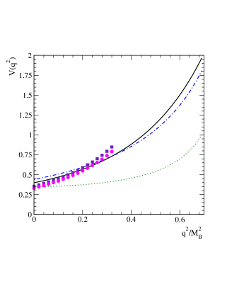
Figure 1: Form factor for $V(q^{2})$ as a fuction of $q^{2}/M_{B}^{2}$. The curve with squares (circles) stands for the PQCD calculation with $\omega_{B}=0.40\ (0.42)$ and the solid curve denotes the minimal values in the LCSR [38], while the dash-dotted and dotted ones represent the results of the QM and LFQM, respectively.

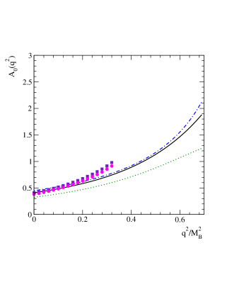
Figure 2: Same as Figure 1 but for $A_{0}(q^{2})$.

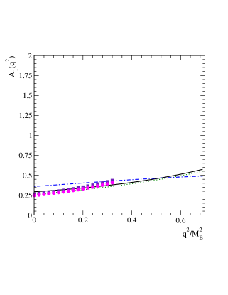
Figure 3: Same as Figure 1 but for $A_{1}(q^{2})$.

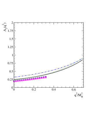
Figure 4: Same as Figure 1 but for $A_{2}(q^{2})$.

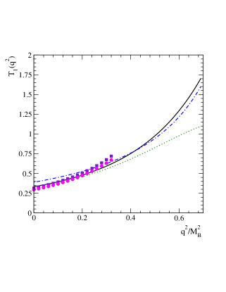
Figure 5: Same as Figure 1 but for $T_{1}(q^{2})$.

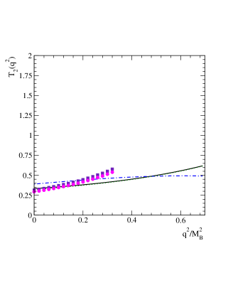
Figure 6: Same as Figure 1 but for $T_{2}(q^{2})$.

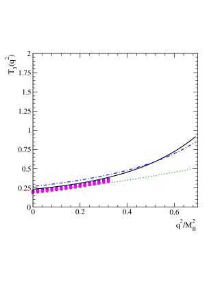
Figure 7: Same as Figure 1 but for $T_{3}(q^{2})$.

In Figures 1-7, we display the form factors $V(q^{2})$, $A_{0,1,2}(q^{2})$, and $T_{1,2,3}(q^{2})$ as functions of $s=q^{2}/M_{B}^{2}$, in the LCSR, QM, LFQM, PQCD (I), and PQCD (II), representing by the solid, dash-dotted, dotted, square and circle curves, respectively.

4.2 Differential decay rates

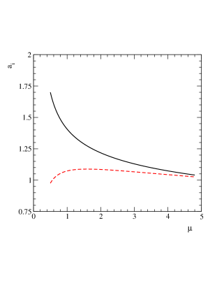
Figure 9: Wilson coefficients as a function of $\mu$ normalized by themselves at $\mu=m_{b}$. The solid and dashed curves are for $a_{7}=C_{7}(\mu)/C_{7}(m_{b})$ and $a_{9}=C_{9}(\mu)/C_{9}(m_{b})$, respectively.

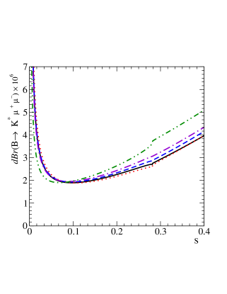
Figure 10: Differential decay rate of $B\to K^{*}\mu^{+}\mu^{-}$ for different $\mu$ scales. The dotted, dashed, dash-dotted, double-dot-dashed curves stand for $\mu=1.3$, $1.5$, $1.7$, and $5.0$ GeV, respectively, while the solid one expresses the result of the full PQCD formalism.

We now present the dilepton invariant mass distributions for $B\to K^{*}\ell^{+}\ell^{-}$ by integrating all angular dependence in the phase space. The distribution for the decay mode with a muon pair in various QCD approaches is shown in Figure 8, where (a) and (b) represent the results with and without resonant effects, respectively. From the figures, we find that the PQCD results are consistent with the minimal ones in the LCSR approach due to similar form factors in the lower $q^{2}$ region in both models. Here, we have set that all WCs are involved at the $m_{b}$ scale for all QCD approaches except the PQCD one. As emphasized in Sec. III, in the PQCD formalism WCs should be convoluted with hard parts and meson wave functions of $B$ and $K^{*}$. Due to the hard gluon exchange, with the momentum squared, $|k_{\bot}|^{2}$, being off-shellness in magnitude of $O(\bar{\Lambda}M_{B})$, dominated in the fast recoil region, the PQCD approach involves a lower scale [26, 22]. As a consequence, even using the concept of the naive factorization, where the decay amplitude is expressed by the product of the WC and the corresponding form factor, the typical scale $t_{0}$ in the PQCD should be much less than $M_{B}$ or $M_{B}/2$. To illustrate the scale dependent on the WCs, we display the $C_{7}(\mu)$ and $C_{9}(\mu)$, renormalized by themselves at $m_{b}$, as functions of $\mu$-scale in Figure 9. In Figure 10, we show the decay rate of $B\to K^{*}\mu^{+}\mu^{-}$ with the relevant WCs fixed at $t_{0}=1.3$, $1.5$, $1.7$ and $5.0$ GeV, respectively. From the figure, we find that the result with $t_{0}=1.3$ GeV is compatible with that from the formal PQCD approach. Similar conclusion is also expected for the electron mode.

4.3 Physical observables

Because the numerical values of ${\cal A}_{i}(q^{2})$ are similar to $\varepsilon_{i}(q^{2})$, in the following numerical calculations, without loss of generality we concentrate on $\varepsilon_{i}(q^{2})$. Moreover, we will not discuss the contributions from ${\cal O}_{3,4,7,8}$ since they are very small.

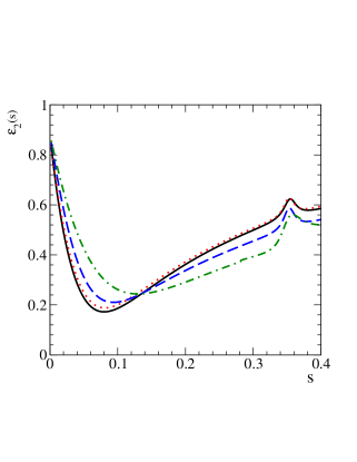
Figure 12: Same as Figure 11 but for $\varepsilon_{2}(q^{2})$.

In Figures 11 and 12, we show the statistical significances of ${\cal O}_{1}$ and ${\cal O}_{2}$, related to the longitudinal and transverse polarizations of $K^{*}$, in various QCD approaches, respectively. From these figures, we see that the differences among different QCD approaches are insignificant, $i.e.$, they are not sensitive to hadronic effects so that they can be used as good candidates to test the SM as well as search for new physics.

In Figures 13 and 14, we display $\varepsilon_{5}(s)$ and $\varepsilon_{6}(s)$ as functions of $s=q^{2}/M_{B}^{2}$, which correspond to the angular distributions of $\cos\theta_{\ell}$ and $\sin 2\theta_{K}$ in Eq. (32) and depend both on $ReC^{eff}_{9}C^{*}_{10}$ and $ReC_{7}C^{*}_{10}$, respectively. From the figures, we see that the zero points of $\varepsilon_{5}$ and $\varepsilon_{6}$ in the PQCD are quite different from others. Hence, by measuring these distributions, especially those zero points, we can distinguish the PQCD results from other QCD models.

To show T violating effects, we concentrate on the T-odd operator of ${\cal O}_{9}$ and consider new CP violating sources beyond the CKM. In the SM, the contribution to $\varepsilon_{9}$ is less than $O(1\%)$. As illustrations, in Figures 15 and 16, we present our results by taking (i) $ImC_{7}=0.25$ and (ii) $ImC_{7}=0.25$ and $ImC_{10}=-0.20$ with the others being the same as those in the SM, respectively. One possible origin of having these imaginary parts is from SUSY where there are many CP violating sources. It is interesting to see that the CP violating effect in Figure 16 can be as large as $30\%$ in these models with new physics. We emphasize that a measurement of such effect is a clear indication of new physics as contrast with the decay rates for which one could not distinguish the non-standard effect due to the large uncertainties in various QCD models as shown in Figure 8. Finally, we note that unlike $\varepsilon_{9}$, $\varepsilon_{7,8}$ receive contributions from the absorptive parts in $C_{9}^{eff}(\mu)$ in the SM and they conserve CP. On the other hand, they are much smaller than $\varepsilon_{9}$ in new physics models such as the ones in (i) and (ii). Due to the uncertainty in the form of $C_{9}^{eff}(\mu)$ in Eq. (25), we shall not discuss them further.

5 Conclusions

We have studied the exclusive decays of $B\to K^{*}\ell^{+}\ell^{-}$ within the framework of the PQCD. We have obtained the form factors for the $B\to K^{*}$ transition in the large recoil region, where the PQCD for heavy $B$ meson decays is reliable. We have found that the form factors at $q^{2}=0$ are consistent with those from most of the other QCD models, in particular, the LEET combined with the HQET and the experimental data on $B\rightarrow K^{*}\gamma$. We have related the angle distributions in the decay chains of $B\rightarrow K^{*}(K\pi)\ell^{+}\ell^{-}$ with 9 physical observables due to the different helicity combinations in $B\rightarrow K^{*}\ell^{+}\ell^{-}$. In particular, we have shown that the T-odd observable can be used to test the SM and search for new physics, which is $<O(1\%)$ and up to $O(10\%)$, respectively. Finally, we remark that to measure such an $10\%$ CP violating effect experimentally at the $1\,\sigma$ level, for example, in $B\to K\pi\mu^{+}\mu^{-}$ one need at least $7.7\times 10^{7}\ B\bar{B}$, which is accessible in the current B factories at KEK and SLAC.

Acknowledgments

We would like to thank K. Hagiwara, W.S. Hou, Y.Y. Keum, and H.N. Li for useful discussions. This work was supported in part by the National Science Council of the Republic of China under Contract Nos. NSC-90-2112-M-001-069 and NSC-90-2112-M-007-040 and the National Center for Theoretical Science.

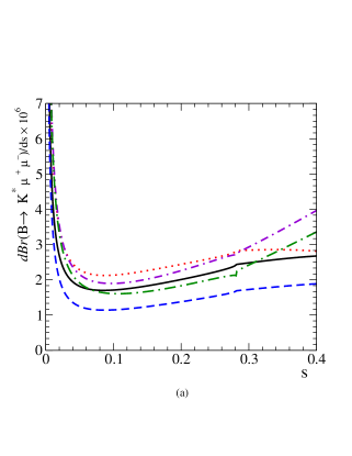
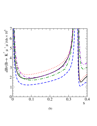
Figure 8: Differential decay rate of $B\to K^{*}\mu^{+}\mu^{-}$ as a function of $s=q^{2}/M^{2}_{B}$. The solid, dotted, and dashed curves stand for the results of the LCSR, QM, and LFQM; the upper and lower dash-dotted ones are those from the PQCD (I) and (II), and (a) and (b) represent the results with and without resonant effects, respectively.

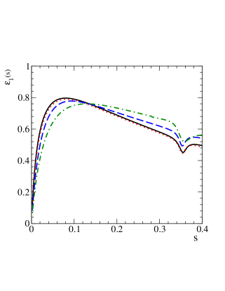
Figure 11: Statistical significance $\varepsilon_{1}(q^{2})$ of ${\cal O}_{1}$ as a function of $s=q^{2}/M^{2}_{B}$. The solid, dotted, dashed, and dash-dotted curves stand for the results of the LCSR, QM, LFQM, and PQCD (I), respectively.

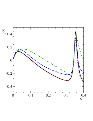
Figure 13: Same as Figure 11 but for $\varepsilon_{5}(q^{2})$.

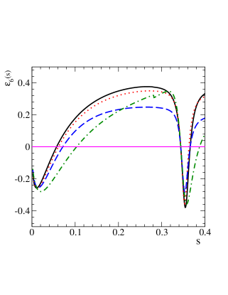
Figure 14: Same as Figure 11 but for $\varepsilon_{6}(q^{2})$.

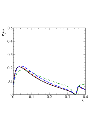
Figure 15: Same as Figure 11 but for $\varepsilon_{9}(q^{2})$ and with $ImC_{7}=0.25$.

Figure 16: Same as Figure 11 but for $\varepsilon_{9}(q^{2})$ and with $ImC_{7}=0.25$ and $ImC_{10}=-2.0$.

References

- [1] CLEO Collaboration, M. S. Alam et. al., Phys. Rev. Lett. 74, 2885 (1995).
- [2] Belle Collaboration, K. Abe et. al., Phys. Rev. Lett. 88, 021801 (2002).
- [3] C.H. Chen and C.Q. Geng, Phys. Rev. D63, 114025 (2001).
- [4] BaBar Collaboration, B. Aubert et. al., hep-ex/0201008.
- [5] Belle Collaboration, H. Yamamoto, talk presented at the fifth KEK topical conference, Nov. 20-22, 2001.
- [6] N. Cabibbo, Phys. Rev. Lett. 10, 531 (1963); M. Kobayashi and T. Maskawa, Prog. Theor. Phys. 49, 652 (1973).
- [7] BABAR Collaboration, B. Aubert et al., Phys. Rev. Lett. 87, 091801 (2001); BELLE Collaboration, A. Abashian et al., Phys. Rev. Lett. 87, 091802 (2001).
- [8] For a recent review, see E. Lunghi and D. Wyler, hep-ph/0109149; and references therein.
- [9] C.H. Chen, C.Q. Geng and J.N. Ng, Phys. Rev. D65, 091502(2002).
- [10] F. Krüger and E. Lunghi, Phys. Rev. D63, 014013 (2000).
- [11] C.Q. Geng and C.P. Kao, Phys. Rev. D57, 4479 (1998); C.H. Chen and C.Q. Geng, Phys. Rev. D64 074001 (2001).
- [12] G.P. Lepage and S.J. Brodsky, Phys. Lett. B87, 359 (1979); Phys. Rev. D22, 2157 (1980).
- [13] N. Isgur and C.H. Llewellyn-Smith, Nucl. Phys. B317, 526 (1989).
- [14] A. Szczepaniak, E. M. Henley, and S. Brodsky, Phys. Lett. B243, 287 (1990).
- [15] R. Akhoury, G. Sterman and Y.P. Yao, Phys. Rev. D50, 358 (1994).
- [16] M. Beneke and T. Feldmann, Nucl. Phys. B592, 3 (2000).
- [17] A. Khodjamirian and R. Ruckl, Phys. Rev. D58, 054013 (1998).
- [18] H.N. Li and G. Sterman, Nucl. Phys. B381, 129 (1992).
- [19] G. Sterman, Phys. Lett. B179, 281 (1986); Nucl. Phys. B 281, 310 (1987).
- [20] S. Catani and L. Trentadue, Nucl. Phys. B327, 323 (1989); Nucl. Phys. B353, 183 (1991).
- [21] H.N. Li, Phys. Rev. D64, 014019 (2001); H.N. Li, hep-ph/0102013.
- [22] Y.Y. Keum, H.N. Li, and A.I. Sanda, Phys. Lett. B504, 6 (2001); Phys. Rev. D63, 054008 (2001).
- [23] C.D. L, K. Ukai, and M.Z. Yang, Phys. Rev. D 63, 074009 (2001).
- [24] C.H. Chen and H.N. Li, Phys. Rev. D63, 014003 (2001).
- [25] E. Kou and A.I. Sanda, Phys. Lett. B525, 240 (2002).
- [26] C.H. Chen, Phys. Lett. B520, 33 (2001).
- [27] B. Melic, Phys. Rev. D59, 074005 (1999).
- [28] C.H. Chen, Y.Y. Keum and H.N. Li, Phys. Rev. D64, 112002 (2001); S. Mishima, Phys. Lett. B521, 252 (2001).
- [29] C.D. L and M.Z. Yang, Eur. Phys. J. C23, 275 (2002).
- [30] C.H. Chen, Phys. Lett. B525, 56 (2002).
- [31] J.C. Collins and D.E. Soper, Nucl. Phys. B193, 381 (1981).
- [32] J. Botts and G. Sterman, Nucl. Phys. B325, 62 (1989).
- [33] H.N. Li, arXiv:hep-ph/0102013.
- [34] T. Kurimoto, H.N. Li, and A.I. Sanda, Phys. Rev. D65, 014007 (2002).
- [35] P. Ball et. al., Nucl. Phys. B529, 323 (1998).
- [36] J. Charles et. al, Phys. Rev. D60, 014001 (1999).
- [37] G. Burdman and G. Hiller, Phys. Rev. D63, 113008 (2001); arXiv:hep-ph/0112063.
- [38] A. Ali et. al., Phys. Rev. D61, 074024 (2000).
- [39] D. Melikhov and B. Stech, Phys. Rev. D62, 014006 (2000).
- [40] H. Y. Cheng et. al., Phys. Rev. D55, 1559 (1997); C.Q. Geng, C.W. Hwang, C.C. Lih, W.M. Zhang, Phys. Rev. D64, 114024 (2001).
- [41] G. Buchalla, A. J. Buras and M. E. Lautenbacher, Rev. Mod. Phys 68, 1230 (1996).
- [42] N.G. Deshpande, J. Trampetic and K. Panose, Phys. Rev. D39, 1462 (1989).
- [43] C.S. Lim, T. Morozumi, and A.T. Sanda, Phys. Lett. B218, 343 (1989).
- [44] A. Ali, T. Mannel, and T. Morozumi, Phys. Lett. B273, 505 (1991).
- [45] P.J. O’Donnell and K.K.K. Tung, Phys. Rev. D43, R2067 (1991).
- [46] F. Krüger and L.M. Sehgal, Phys. Lett. B380, 199 (1996).
- [47] Z. Ligeti and M. B. Wise, Phys. Rev. D 53, 4937 (1996).
- [48] G. Burdman, Phys. Rev. D 57, 4254 (1998).
- [49] C.H. Chen and C.Q. Geng, arXiv:hep-ph/0205306, to appear in Phys. Rev. D.
- [50] C.S. Kim et. al., Phys. Rev. D62, 034013 (2000); C. S. Kim, Y. G. Kim and C. D. Lü, ibid. D 64, 094014 (2001); T. M. Aliev et. al., Phys. Lett. B511, 49 (2001); Q. S. Yan et. al., Phys. Rev. D 62, 094023 (2000).
- [51] F. Kruger et. al., Phys. Rev. D 61, 114028 (2000) [Erratum-ibid. D 63, 019901 (2000)].
- [52] Y. Grossman and D. Pirjol, JHEP 0006, 029 (2000).
- [53] M. Bauer and M. Wirbel, Z. Phys. C 42, 671 (1998).
- [54] C.H. Chen, Y.Y. Keum and H.N. Li, arXiv:hep-ph/0204166.
- [55] BELLE Collaboration, H. Yamamoto, talk presented at the fifth KEK topical conference, Nov. 20-22, 2001.