Study of relativistic bound states for scalar theories in Bethe-Salpeter and Dyson-Schwinger formalism

Abstract

The Bethe-Salpeter equation for Wick-Cutkosky like models is solved in dressed ladder approximation. The bare vertex truncation of the Dyson-Schwinger equations for propagators is combined with the dressed ladder Bethe-Salpeter equation for the scalar S-wave bound state amplitudes. With the help of spectral representation the results are obtained directly in Minkowski space. We give a new analytic formula for the resulting equation simplifying the numerical treatment. The bare ladder approximation of Bethe-Salpeter equation is compared with the one with dressed ladder. The elastic electromagnetic form factors is calculated within the relativistic impulse approximation.

I Introduction

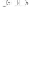
Figure 1: Diagramatical representation of the BSE for the bound state vertex function.

In the Quantum Field Theory the two body bound state is described by the three-point bound state vertex function or, equivalently, by Bethe-Salpeter (BS) amplitudes, both of them are solutions of the corresponding (see Fig. 1) covariant four-dimensional Bethe-Salpeter equations (BSE)BETHE . Up to now most of the studies were restricted to the case when irreducible interaction kernel is approximated by (sum of) single particle exchanges. In this so called ladder approximation the scattering matrix is given by the sum of the generated ladders. It is known, that such approximation is not sufficient when more realistic models are considered ROBERTS , SMEKAL , SCHMIDT . To move beyond this approximation one is in practice confined to the use of some phenomenological Ansatze. (In hadronic physic, these Ansatze are very often made already at the level of two point correlators. For modeling of the gluon propagator in the context of BSE and Dyson-Schwinger equations (SDE), see for instance MARIS ).

Here we are considering some simple scalar models. An extensive review of BS studies in scalar theories (with at most cubic and non-derivative interaction) can be found in Ref. Nakan , SETO . The various improvements of simple ladder kernel have been considered, in particular, including the self-energy effects KUSAK3 , AHLIG or contributions from crossed box diagrams THEUSL . The study of the influence on the bound state spectrum following from the infinite resummation of certain ladder and crossed-box diagrams can be found in the paper TJON2 . Furthermore, there is a number of interesting papers on the solution of Wick-Cutkosky models (with zero mass of the exchanged particle). These solutions employ various effective techniques like the point form of relativistic quantum mechanics DEPLANK , variational calculations DAREWYCH or the light front dynamics MILLER .

The standard approach to determine the spectrum and the BS vertex makes use of partial wave decomposition which reduces four-dimensional integral equation into the two-dimensional one. The alternative more recently exploited treatment is based on the $O(4)$ hyperspherical expansion TJON . In this approach the BSE is transformed into an infinite set of one-dimensional integral equations. Notable advantage of this approach is a good numerical convergence and easy identification of excited bound states spectra.

Very often, the ladder BSE’s are solved with the help of the so-called Wick rotation WICK . However, the backward analytical continuation is quite difficult even for the ladder approximation, while for more complicated cases its proper implementation is unclear or at least highly non-trivial.

In this work we follow the method of solving the BSE directly in Minkowski space KUSAK3 , KUSAK1 , FULTON , in which the problems associated with Wick rotation do not arise. The method is based on utilization of generalized spectral representation for n-point Green functions in quantum field theory NAKANATO . In this treatment the BSE written in momentum space is converted into a real integral equation for a real weight function with number of independent variables dependent on details of the model. We extend the earlier work KUSAK3 first to the case with unequal masses of constituents. This then allows us to treat the ladder BSE in which all propagators (of constituents and of the exchanged particle) are fully dressed. This is achieved by the implementation of Lehmann representation of the propagator:

$$G(p^{2}) = \int\limits d\omega\,\tilde{\sigma}(\omega)D(p;\omega)\,,$$

$$D(p;\omega)=\frac{1}{p^{2}-\omega+i\epsilon}\quad \quad\tilde{\sigma}(\omega)=R\,\delta(\omega-m^{2}_{pole})+\sigma(\omega)\,.$$ ; (1)

where $\sigma(\omega)$, which is a smooth function, nonzero above a threshold, is determined by the Dyson-Schwinger equations (DSE). In the pole term we can take $R=1$, a choice corresponding to the conventional on-shell renormalization scheme ($G$ has a unit residuum when momentum approaches a simple pole at physical mass).

To account for the effect of self-energy we transform the momentum BSE to the form suitable for complementary solution together with the appropriate DSE for propagators. Note here, that the perturbative one loop contribution has been already considered in KUSAK3 and certain Euclidian version of this problem has also been investigated AHLIG . In qualitative agreement with AHLIG we have found that the critical value of coupling gives the domain of applicability of BSE (at least in its ladder approximation). The couplings below critical one allow only solutions for relatively weakly bound states. It is even more interesting that the effect of the propagator dressing on bound state spectra is rather small. In comparison with the bare ladder approximation the same binding energy is then achieved with the coupling smaller by about several per cents, even for values of the coupling close to the critical one.

Clearly, when we take some or even all particle propagators dressed, the number of spectral integrations increases. Note here, that up to the rather exotic case of massless Wick-Cutkosky model the appropriate solution is not known analytically but must be found numerically. Mainly due to this reason we re-formulate the equation obtained by Kusaka et al KUSAK3 and we offer the solution where the appropriate integral kernel is free of any additional numerical integration (see Appendix of Ref. KUSAK3 for the original solution). The elimination of this numerical integration then not only improves numerical accuracy but also reasonably decreases the CPU time.

To see explicitly the effect of radiative corrections we compare the derssed BSE results with its bare ladder approximation. We set the parameters of our model to that used in Refs. TJON and KUSAK1 , to compare the bare ladder solutions to those obtained before in KUSAK3 , TJON , KUSAK1 .

Having solved equations for spectral functions, one can determine the BS amplitudes in an arbitrary reference frame. This makes this technique suitable for calculations of response to an external fields. In section IV. we briefly introduce the formulas defining the elastic charge form factor $G(Q^{2})$ in relativistic impulse approximation (RIA). Although the elastic form factor represents a simple dynamical observable, its Minkowskian calculation represents nontrivial task. For this purpose we consider the (massive) Wick-Cutkosky model given by Lagrangian gauged as follows:

$${\cal L} = (D^{\mu}\phi_{1})^{+}D_{\mu}\phi_{1}+\frac{1}{2}\partial_{\mu}\phi_{2}\partial^{\mu}\phi_{2}+\frac{1}{2}\partial_{\mu}\phi_{3}\partial^{\mu}\phi_{3}-\frac{1}{4}F_{\mu\nu}F^{\mu\nu}-V(\phi_{i})\,,$$

$$V(\phi_{i}) = \left(m_{1}^{2}+g\phi_{3}\right)\phi_{1}^{+}\phi_{1}+\left(\frac{m_{2}^{2}}{2}+{g\over 2}\,\phi_{3}\right)\phi^{2}_{2}+\frac{1}{2}m_{3}^{2}\phi_{3}^{2}\,,$$ (2)

where covariant derivative is $D_{\mu}=\partial_{\mu}-ieA_{\mu}$. In our form factor calculations the effects of scalar dressing was not taken into account, since it would significantly increase computational complexity of the problem. Furthermore, it is assumed that $e<<g$ which implies that the interaction of the charged particle field $\phi_{1}$ with the electromagnetic field can be treated perturbatively. As in Ref. AHLIG , we have chosen the same coupling constant for interaction of the field $\phi_{3}$ with the fields $\phi_{1}$ and $\phi_{2}$. The form factors were calculated for several sets of masses of constituent and exchanged particles.

II Dressed Ladder Bethe-Salpeter Equation

The BS amplitude for bound state $(\phi_{1},\phi_{2})$ in momentum space is defined through the Fourier transform of

$$\langle 0|T\phi_{1}(x_{1})\phi_{2}(x_{2})|P\rangle=e^{-iP\cdot X}\langle 0|T\phi_{1}(\eta_{2}x)\phi_{2}(-\eta_{1}x)|P\rangle=e^{-iP\cdot X}\int{d^{4}p\over(2\pi)^{4}}e^{-ip\cdot x}\Phi(p,P)\ ,$$ (3)

where $X\equiv\eta_{1}x_{1}+\eta_{2}x_{2}$ and $x\equiv x_{1}-x_{2}$, so that $x_{1}=X+\eta_{2}x$, $x_{2}=X-\eta_{1}x$. Here $p_{1,2}$ are the four-momenta of particles corresponding to the fields $\phi_{1,2}$ that constitute the bound state $(\phi_{1},\phi_{2})$. The total and relative momenta are then given as $P=p_{1}+p_{2}$ and $p=(\eta_{2}p_{1}-\eta_{1}p_{2})$, respectively, and $P^{2}=M^{2}$, where $M$ is mass of the bound state. Finally, $P\cdot X+p\cdot x=p_{1}\cdot x_{1}+p_{2}\cdot x_{2}$. From now on we will put $\eta_{1}=\eta_{2}=1/2$, which corresponds to the usual separation of center of mass motion for equal mass case, but can be also employed for unequal masses (although $X$ is then not the coordinate of the center of mass).

Introducing the BS vertex function $\Gamma=iG_{1}^{-1}G_{2}^{-1}\Phi$, the homogeneous BSE for S-wave bound state reads

$$\Gamma(p,P)=i\int{d^{4}k\over(2\pi)^{4}}\,V(p,k;P)G_{1}(k+P/2)G_{2}(-k+P/2)\Gamma(k,P)\,.$$ (4)

The bound states appear as poles of the scattering matrix. The normalization condition for the BS vertex function follows from the requirement that the pole appropriate to a given bound state is a simple one:

$$2iP^{\mu}\ = \int\frac{d^{4}p}{(2\pi)^{4}}\int\frac{d^{4}k}{(2\pi)^{4}}\bar{\Gamma}(k,P)\left[(2\pi)^{4}\delta^{4}(p-k)\left(\frac{\partial}{\partial P_{\mu}}G_{1}(p_{1})G_{2}(p_{2})\right)\right.$$ (5)

$$\left.+i\,G_{1}(p^{\prime}_{1})G_{2}(p^{\prime}_{2})\,\left(\frac{\partial}{\partial P_{\mu}}V(p,k;P)\right)\,G_{1}(p_{1})G_{2}(p_{2})\,\right]\,\Gamma(p,P)\,,$$

where $\bar{\Gamma}(p,P)$ is the conjugate of $\Gamma(p,P)$ and $p_{1,2}=\pm p+P/2,p^{\prime}_{1,2}=\pm k+P/2$ (for the details see e.g. Ref. Nakan ).

In this work we do not solve the BSE with most general irreducible scattering kernel $V$ (the most general structure of the kernel $V$ written in terms of its Perturbation Theory Integral Representation (PTIR) can be found in Ref. KUSAK3 or NAKANATO ). Here we restrict ourselves to the case of dressed ladder approximation with $\phi_{3}$-exchange, in which $V(p,k;P)=g^{2}G_{3}(t)$, where $t$ denotes the usual Mandelstam variable $t=(p-k)^{2}$. Note that for the bound state of particles $(\phi_{1},\phi_{2})$ only the $t$-channel interaction above is effective, whereas for the bound state of $(\phi_{i},\phi_{i}),i=1,2$ one has to consider also possible $u$ and $s$ channel diagrams. In the present work we study the case $(\phi_{1},\phi_{2})$ due to its simplicity and leave the other cases for discussion elsewhere. Let us also recall that in the (dressed) ladder approximation, defined by the exchange of chargeless scalar $\phi_{3}$, the photon coupling to $\phi_{1}$ alone (one particle current, or in other words RIA) is by itself gauge invariant, when taken between the corresponding solutions of BSE. And the normalization condition (5) in this approximation reduces to the condition $G(Q^{2})=1$. We will solve the BSE for massive constituents ($m_{1,2}>0$) and $m_{3}\geq 0$, the invariant mass of the bound state satisfies $0\leq P^{2}<(m_{1}+m_{2})^{2}$.

Taking the dressed kernel and the full propagators of constituent particles into account, the rhs of BSE (4) can be written as

$$ig^{2}\prod_{i=1}^{3}\int d\alpha_{i}\,\tilde{\sigma}(\alpha_{i})\int{d^{4}k\over(2\pi)^{4}}D(k+P/2;\alpha_{1})D(-k+P/2;\alpha_{2})D(k-p;\alpha_{3})\Gamma(k,P)\,.$$ (6)

The interesting unequal-mass ladder case of Ref. FUKUI is also described by Eq.(6), although $\eta_{1}=\eta_{2}=1/2$ and $p$ and $k$ are not relative momenta. Since the dependence on momenta in (6) is explicit, one might always re-scale $\Gamma(p,P)$ to proper relative momentum.

The integral representation for the BS vertex function may be written as NAKANATO

$$\Gamma(p,P)=\int\limits_{-1}^{1}dz\,\int\limits_{\alpha_{min}(z)}^{\infty}d\alpha\,\,\frac{\rho^{[n]}(\alpha,z)}{[\alpha-(p^{2}+zp\cdot P+P^{2}/4)-i\epsilon]^{n}}\,\,.$$ (7)

The positive integer $n$ represents a free parameter without clear physical meaning. One can take advantage of this freedom of choice to pick up $n$ so that the numerical solutions of integral equations for spectral functions are made more stable. The spectral functions $\rho^{[n]}(\alpha,z)$ for different $n$ can be related by integration over $\alpha$ by parts. Kusaka et al KUSAK3 choose $n=2$ for their numerical solution of the BSE, we adopt the same value in this paper.

The bare (symmetric) Wick-Cutkosky model corresponds to the choice: $\alpha_{1}=\alpha_{2}=m^{2}$, the exchanged boson is massless ($\alpha_{3}=0$) and no radiative corrections are considered. This model is particularly interesting because it is the only example of the nontrivial BSE which is solvable exactly WICK . For this model, there is no freedom in choice of $n$ and (for the S-wave bound state) the expression (7) reduces to the one dimensional PTIR:

$$\Gamma(p,P)=\int\limits_{-1}^{1}dz\,\frac{\rho(z)}{m^{2}-(p^{2}+zp\cdot P+P^{2}/4)-i\epsilon}\,\,.$$ (8)

Using a technique similar to the one used in ref. KUSAK3 , the BSE can be converted to the following real integral equation for the real spectral function:

$$\rho^{[n]}(\alpha^{\prime},z^{\prime})=\lambda\int\limits_{-1}^{1}dz\int\limits_{\alpha_{min}(z)}^{\infty}d\alpha\,\,V^{[n]}(\alpha^{\prime},z^{\prime};\alpha,z)\,\rho^{[n]}(\alpha,z)\,,$$ (9)

where we denoted $\lambda=g^{2}/(4\pi)^{2}$. The derivation is presented in the Appendix A, where the explicit expressions for particular choices $n=1,2$ are given. The central results of this work are expressions obtained for $V^{[n]}$, which are simpler that the ones presented in Ref. KUSAK3 . No additional integration is required which decreases the computer time necessary for numerical calculation. Besides, our formulas hold also for unequal masses of the constituents. The extension (together with above mentioned simplification) to the case of more complicated scattering kernel is not so straightforward, but we believe that it is possible. Note also, that due to the property of solid harmonic with respect to the integration over the momentum the presented procedure can easily be generalized for the bound state with non-zero spin (here, the total orbital momentum)KUSAK3 .

A bound state with equal composite masses is described by the vertex function $\Gamma$ which is symmetric under the transformation $P\cdot p\rightarrow-P\cdot p$. In terms of the weight function this symmetry reads $\rho(\alpha,z)=\rho(\alpha,-z)$. However, there are solutions that do not respect this symmetry even in the case of equal masses. These are usually called ghost solutions and the appropriate amplitudes have a negative norm. Such solutions are often considered to be nonphysical and it is supposed that they point at inner inconsistency in description of relativistic bound states within the BS formalism, at least in the ladder approximation. At this place, it is important to mention that the Lagrangian (I) describes the models that are a subset of theories with potentials unbounded from below and in very strict sense they are discarded due to the vacuum instability. On the other hand one can assume, at least for sufficiently small couplings the existence of local minima of the potentials is sufficient to support of the existence of ground state of the theory. While in the large coupling regime, say for $g/m>>1$ no reasonable physics can be learned from the perturbation theory and/or from equation like ladder BS by itself. To conclude, we note that such ideas are supported by at least two facts. The ghost BS solutions do appear only for a large value of $\lambda$. Furthermore, from the Dyson-Schwinger study we know that the scalar theory studied here makes sense only up to the certain critical coupling, see e.g. AHLIG , SUPER .

The important question arises, what is the validity of the full theory when renormalization is properly taken into account. Although the quantitative answer lies beyond the approximations used in this article and requires more careful investigation, we make a simple attempt to find the domain in which self-consistent solutions of the BSE and Dyson-Schwinger equations (within the framework of reasonable approximations) exist. Furthermore, we inquire an influence of scalar propagator dressing on the solution of the BSE for the bound states.

III Dressing propagators by the Dyson-Schwinger equations

The solution of the DSE for the scalar models with the help of spectral decomposition will be discussed in detail in our forthcoming paper SUPER . Here we give only brief presentation of the DSE in bare vertex approximation, their renormalization, re-arrangement in terms of the spectral function and some properties of solutions, important for our further discussion of the BSE. In this section we assume $m_{3}<m_{1}+m_{2}$, so that the propagator of the exchanged particle $\Phi_{3}$ has an isolated physical pole.

By dressing of the scalar propagators in our study of BSE we mean only the dressing due to the “strong” interaction between scalars, the coupling to the electromagnetic field is neglected. Let us now write the strong interaction part of our Lagrangian (I) in terms of bare, unrenormalized quantities (fields and coupling constants), labeled by subscript ”0”:

$${\cal L}_{strong}=-g_{01}\,\phi_{01}^{+}\phi_{01}\phi_{03}-{g_{02}\over 2}\,\phi_{02}^{2}\phi_{03}\,.$$ (10)

In the previous section we have chosen the strength of of both couplings to be the same. Here, we distinguish the bare couplings, anticipating that they are renormalized by different amounts (see below).

The kinetic terms are parametrized by the unrenormalized masses $m_{0i}$. These masses undergo the infinite mass renormalization

$$m_{0i}^{2}=m_{i}^{2}-\delta m^{2}_{i}\,,\quad i=1,2,3\,.$$ (11)

To re-scale the residuum of the full propagators to unity, we will complement the infinite mass renormalization by the finite (since the model is superrenormalizable) renormalization of the fields and coupling constants

$$\phi_{0i}=\sqrt{Z_{i}}\,\phi_{i}\,,\quad i=1,2,3\,,\quad\quad g_{0i}=\frac{1}{Z_{i}\sqrt{Z_{3}}}\,g_{i},\quad i=1,2\,.$$ (12)

That is, we will employ below the on shell renormalization scheme in which the propagators have unit residua when momentum approaches its mass shell value $p^{2}\rightarrow m^{2}$.

In this paper we consider the Dyson-Schwinger equations in the simplest approximation in which the proper vertices are replaced by the bare ones $\Gamma_{oi}=g_{oi}$. Then, the DSE in their unrenormalized form read

$$G_{0i}^{-1}\left(p\right) = p^{2}-m_{0i}^{2}-\Pi_{0i}(p^{2})\,,\quad\quad i=1,2,3$$

$$\Pi_{0i}(p^{2}) = i\,g_{0i}^{2}\int\frac{d^{4}q}{\left(2\pi\right)^{4}}\,G_{03}\left(p-q\right)G_{0i}\left(q\right)\,,\quad\quad\quad i=1,2$$

$$\Pi_{03}(p^{2}) = i\int\frac{d^{4}q}{\left(2\pi\right)^{4}}\,\sum_{i=1,2}g_{0i}^{2}G_{0i}\left(p-q\right)G_{0i}\left(q\right)\,,$$ (13)

where $G_{0}(p)$ is the Fourier transform of the full unrenormalized propagator $G_{0i}(x-y)=$ $<0|T\phi_{0i}(x)\phi_{0i}(y)|>$ and $\Pi_{0i}$ is the corresponding self-energy.

Under the field strength renormalization the propagators scale like $G_{0i}=Z_{i}G_{i}$. Multiplying the equations for $G_{0i}^{-1}$ in (III), defining $\Pi_{i}=Z_{i}\Pi_{0i}$ and making use of (12), one gets the re-scaled DSE

$$G_{i}^{-1}(p^{2}) = Z_{i}(p^{2}-m_{0i}^{2})-\Pi_{i}(p^{2})\,,$$

$$\Pi_{i}(p^{2}) = i\,g_{i}^{2}\int\frac{d^{4}q}{\left(2\pi\right)^{4}}\,G_{3}\left(p-q\right)G_{i}\left(q\right)\,,\quad\quad\quad i=1,2$$

$$\Pi_{3}(p^{2}) = ig^{2}\int\frac{d^{4}q}{\left(2\pi\right)^{4}}\,\sum_{i=1,2}G_{i}\left(p-q\right)G_{i}\left(q\right)\,.$$ (14)

The renormalization of proper self-energies proceeds by double subtraction:

$$\Pi_{iR}(p^{2})=\Pi_{i}(p^{2})-\Pi_{i}(m^{2})-(p^{2}-m_{i}^{2})\,\frac{d\Pi_{i}(p^{2})}{dp^{2}}|_{p^{2}=m_{i}^{2}}\,\,.$$ (15)

Identifying the appropriate renormalization constants (11,12)

$$\delta m^{2}_{i}=\Pi_{i}(m_{i}^{2})/Z_{i}\,,\quad\quad Z_{i}=1+\frac{d\Pi_{i}(p^{2})}{dp^{2}}|_{p^{2}=m_{i}^{2}}\,,$$ (16)

we can immediately write the full propagator in terms of finite physical quantities

$$G_{i}^{-1}\left(p\right)=p^{2}-m_{i}^{2}-\Pi_{iR}(p^{2})\,,\quad i=1,2,3\,.$$ (17)

The DSE for the renormalized self-energies are given by (14) and subtraction (15).

For the purpose of our BS calculation, we now fix the renormalized couplings and masses as follows

$$g_{1}=g_{2}\equiv g;\quad m_{1}=m_{2}\equiv m;\quad m_{3}=\frac{m}{2}$$ (18)

where $g$ is coupling constant from (I). That is, we will compare the solutions of the BSE for the bare and dressed ladder kernel taken for the same numerical value of unrenormalized and renormalized coupling constant, respectively. The masses are fixed to allow comparison with some of the results of Refs. KUSAK1 ; KUSAK3 ; TJON .

Now, it is straightforward task to evaluate the spectral representation of the renormalized self-energy. Lehmann representation (with unit residuum) for $G_{i}$ reads:

$$G_{i}(p^{2})=\int_{0}^{\infty}ds\frac{\tilde{\sigma}(s)}{p^{2}-s+i\epsilon}\,,\quad\quad\tilde{\sigma}(s)=\delta(m_{i}^{2}-s)+\sigma(s)\,,$$ (19)

Notice that functions $\sigma_{i},i=1,2$, have the thresholds at $m_{i,th}=(m_{i}+m_{3})^{2}=2.25m^{2}$, whereas the function $\sigma_{3}$ has the threshold at $m_{3,th}=(m_{1}+m_{2})^{2}=4m^{2}$. Analogously, for the for self-energies:

$$\Pi_{iR}(p^{2})=\int_{m_{i,th}}^{\infty}d\alpha\,\frac{\rho_{\pi i}(\alpha)}{p^{2}-\alpha+i\epsilon}\frac{(p^{2}-m^{2})^{2}}{(\alpha-m^{2})^{2}}\,.$$ (20)

The spectral representation for $\Pi_{R}$ explicitly satisfies $\Pi_{R}(m^{2})=\Pi_{R}^{\prime}(m^{2})=0$ following from (15). Rewriting now the relation between $G$ and $\Pi$ in the form $G=D+D\Pi G$ ($D$ being the free propagator with the physical mass) and taking its imaginary part, we arrive to the first relation between the spectral functions $\sigma$ and $\rho$:

$$\sigma_{i}(\omega)=\frac{\rho_{\pi_{i}}(\omega)}{(\omega-m_{i}^{2})^{2}}+(\omega-m_{i}^{2})\,P\int{d\alpha\over\omega-\alpha}\left[\frac{\sigma_{i}(\omega)\rho_{\pi_{i}}(\alpha)}{(\alpha-m_{i}^{2})^{2}}+\frac{\sigma_{i}(\alpha)\rho_{\pi_{i}}(\omega)}{(\omega-m_{i}^{2})^{2}}\right]\,,\quad i=1,2,3\,,$$ (21)

where $P\int$ stands for principal value integration. All the functions in (21) are positive and regular above the perturbative thresholds and identically equal to zero elsewhere.

Substituting the spectral representations (19) into the DSEs (14), making the subtraction as in (15) and comparing to the lhs in the form of (20), one gets after lengthy algebra:

$$\rho_{\pi_{i}}(\omega) = \lambda\,\int d\alpha\,d\beta\,B(\alpha,\beta;\omega)\tilde{\sigma}_{3}(\alpha)\tilde{\sigma}_{i}(\beta)\,,\quad\quad i=1,2\,,$$

$$\rho_{\pi_{3}}(\omega) = \lambda\,\sum_{i=1,2}\int d\alpha\,d\beta\,B(\alpha,\beta;\omega)\tilde{\sigma}_{i}(\alpha)\tilde{\sigma}_{i}(\beta)\,,$$ (22)

where $\lambda=g^{2}/(4\pi)^{2}$ and the function $B(\alpha,\beta;\omega)$ is related to the Källen function $\lambda$ as follows:

$$B(\alpha,\beta,\omega) = \frac{\sqrt{\lambda(\alpha,\beta,\omega)}}{\omega}\,\Theta\left(\omega-(\sqrt{\alpha}+\sqrt{\beta})^{2}\right)\,,$$

$$\lambda(\alpha,\beta,\omega) = \alpha^{2}+\beta^{2}+\omega^{2}-2\alpha\beta-2\alpha\omega-2\beta\omega,.$$ (23)

Before the numerical treatment the explicit integration- separating the $\delta$-function parts of Lehmann weights $\tilde{\sigma}$- has to be performed.

Equations (21,III) constitute the closed system of integral equations for spectral functions which can be solved numerically by iterations without any additional approximation. So obtained dressed propagators have been used when solving the Bethe-Salpeter equation. The results are discussed in the section V. Before leaving this section we review some important features of our solutions of DSE.

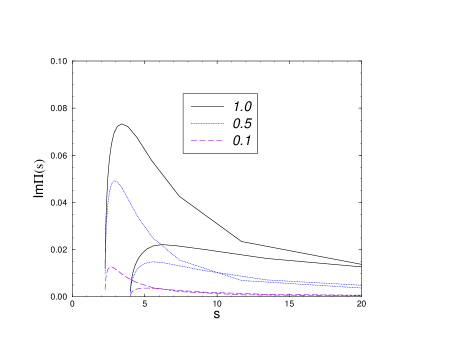
Figure 2: The imaginary part of the renormalized propagators for different values of coupling $\tilde{\lambda}$, calculated from the DSE in bare vertex approximation. Upper curves are for particles $\Phi_{1,2}$ (which have identical self-energies, lower ones for particle $\Phi_{3}$ .)

The behavior of the imaginary parts of propagators– the Lehmann functions $\sigma_{i}(\alpha)$– for fields $\Phi_{1,2,3}$ is shown at Fig. 2.

The renormalization constant $Z_{i}$ are calculated from the relation

$$Z_{i}=1-\int d\alpha\,\frac{\rho_{i}(\alpha)}{(\alpha-m_{i}^{2})^{2}}\,.$$ (24)

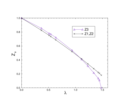
Figure 3: The dependence of field strength renormalization constants on the coupling $\tilde{\lambda}$.

From the Fig.3 we can see that the field renormalization constant $Z_{1,2}$ changes sign from positive to negative at some critical point $\tilde{\lambda}_{crit}=g_{crit}^{2}/(4\pi m)^{2}\simeq 1.5\pm 0.1$, where the error reflects the difficulty of making the numerical estimate of the value for which the solution cannot be found and the dimensionless coupling is defined as $\tilde{\lambda}=\lambda/m^{2}$ . We did not find any numerical solutions of DSE for couplings larger than $\tilde{\lambda}_{crit}$. It is reasonable to suppose that the quanta associated with the fields $\phi_{1,2}$ do not describe physical particles when $\tilde{\lambda}>\tilde{\lambda}_{crit}$.

IV Elastic Electromagnetic Form Factor

The electromagnetic form factors parameterize the response of bound systems to external electromagnetic field. The calculation of these observables within the BS framework proceeds along the Mandelstam’s formalism MANDEL . For the elastic scattering on the S-wave bound state, ($P_{i}^{2}=P_{f}^{2}=M^{2}$) the current conservation implies the parameterization of the current matrix element $G^{\mu}$ in terms of the single real form factor $G(Q^{2})$

$$G^{\mu}(P_{f},P_{i})=G(Q^{2})(P_{i}+P_{f})^{\mu}\,.$$ (25)

The elastic electromagnetic form factor $G(Q^{2})$ depends only on the square of photon incoming momentum $q$ and we use the usual SLAC convention $Q^{2}=-q^{2}$, so that $Q^{2}$ is positive for elastic kinematics.

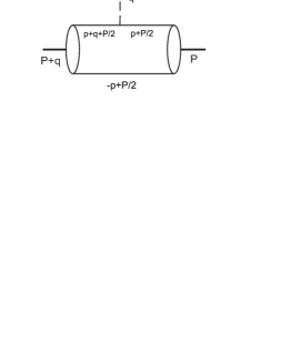
Figure 4: Diagrammatic representation of the e.m.  current bound state matrix element.

The matrix element of the current in relativistic impulse approximation (RIA) is diagrammatically depicted in Fig. 4. In this paper we are not taking into account the dressing of the scalar propagators when calculating the charge form factor. Then, the matrix element is given in terms of the BS vertex functions as

$$G^{\mu}(P+q,P) = i\,\int\frac{d^{4}k}{(2\pi)^{4}}\,\bar{\Gamma}(k+\frac{q}{2},P+q)$$ (26)

$$\left[D(p_{f};m_{1}^{2})j_{1}^{\mu}(p_{f},p_{i})D(p_{i};m_{1}^{2})\,D(-k+P/2;m_{2}^{2})\right]\Gamma(k,P)\,,$$

where we denote $P=P_{i}$ and $j_{1}^{\mu}$ represents one-body current for particle $\phi_{1}$, which for the bare particle reads $j_{1}^{\mu}(p_{f},p_{i})=p_{f}^{\mu}+p_{i}^{\mu}$, where $p_{i},p_{f}$ is initial and final momentum of charged particle inside the loop in Fig. 4, i.e., $p_{i}=k+P/2,p_{f}=q+k+P/2$.

We have already mentioned in the previous section, that if the vertex functions $\Gamma$ are solution of the BSE with a kernel corresponding to exchange of single chargeless particle, the RIA defined above is by itself gauge invariant and the normalization condition for the BS amplitudes is equivalent to the normalization $G(0)=1$.

The main result of this paper, as far as charge form factor is concerned, is re-writing of the rhs of Eq. (26) directly in terms of the spectral weights of the bound state vertex function. It allows the evaluation of the form factor by calculating the integral of nonsingular expression, without having to reconstruct the vertex functions $\Gamma(p,P)$ from their spectral representation. The derivation of this integral involves some lengthy algebra and is relegated to Appendix B.

V Numerical Results

V.1 Bare Ladder BSE

We have solved the bare ladder BSE for symmetric ($m_{1}=m_{2}=m$) scalar theory with bare ladder kernel

$$V(p,k,P)=V(p-k)=\frac{g^{2}}{(p-k)^{2}-m^{3}_{2}}\,,$$ (27)

and bare constituent propagators $G_{i}(p_{i})=D_{i}(p_{i},m_{i})$ by iterations of the integral equation for spectral functions. The standard procedure was followed: after fixing the bound state mass ($P^{2}$) we looked for the solution by iterating spectral function for fixed dimensionless ”coupling strength” $\tilde{\lambda}\equiv g^{2}/((4\pi\,)^{2}m^{2})$. If the iterations failed– measure being both the difference of the rhs and lhs of the integral equation and deviation of the auxiliary normalization integral from pre-defined value– we were changing $\tilde{\lambda}$ (halving intervals of successive guesses) till the solution was found.

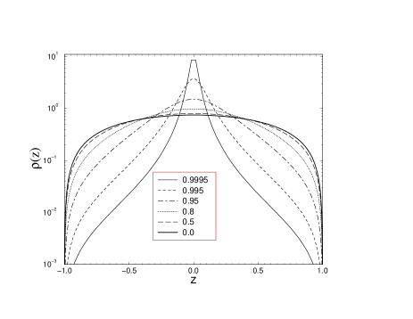
Figure 5: The spectral function $\rho(z)$ of the bound-state vertex in the Wick-Cutkosky model for several values of $\eta=\sqrt{P^{2}}/2m$ .

In case of Wick-Cutkosky model the one dimensional integral equation (A.1) was solved. Although the solution of this one-dimensional integral equation could be found by the inversion of its discretized form, we have tested the iteration procedure (used later also for massive exchange). The equation was discretized by numerical Gauss integration, it appear that it is sufficient to take 40 Gauss point (though the number cited in Table 1 are obtained with 98 points). It is known Nakan that $P^{2}=0$ corresponds to $\tilde{\lambda}=2$ from which our result slightly deviates in the fifth digit. We have also reproduced (up to four published digits) all results for Wick-Cutkosky model from TJON . In the Fig.5 the weight functions are plotted against spectral variable $z$ for several fractions of binding $\eta=\sqrt{P^{2}}/2m$ .

For the massive scalar exchange the two-dimensional integral equations (54,57) were solved. We have found (in agreement with KUSAK3 ) that numerical errors are about one order of magnitude bigger for $n=1$, hence $n=2$ is preferable and only the results with this choice are discussed below.

For numerical solution we discretize integration variables $\alpha$ and $z$ using Gauss-Legendre quadratures (with tangent mapping from $<-1,+1>\rightarrow<\alpha_{min},\infty>$ for $\alpha$ ). The equation (57) is solved on the net of $N=N_{z}*N_{\alpha}$ points which are spread on the rectangle $(-1,+1)*(\alpha_{min},\infty)$. The value $\alpha_{min}$ is given by the support of the spectral function (see the appendix A). We have not optimized the grid during the iteration procedure as it was done in the study KUSAK3 . Instead, we have solved the equation for several different numbers of grid points while keeping fixed the ratio of $N_{\alpha}/N_{z}$ and then extrapolated the results to the “ideal” case with $N_{\alpha}=N_{z}=\infty$. Examples of numerical convergence for some cases of bound states are presented in the Table 2. In the Table 1 we compare our results for $m_{3}=m/2$ with those of ref. KUSAK3 .

Below we show the dependence of charge form factor on the parameters of the model: on the range of interaction characterized by the inverse mass of exchanged meson $m_{3}$ and on the strength of forces which bind the particles together. To calculate the form factors we first have to solve the BSE for chosen sets of parameters. We vary the parameters as follows:

1. First we solve the BSE for several bound state masses $P^{2}$ keeping the ratio $m_{3}/m$ fixed

2. Then we vary the mass of the exchanged meson, keeping the masses of all studied bound states fixed (our choice is $\eta=\sqrt{P^{2}}/(2m)=0.5$) and determining the corresponding coupling strengths $\tilde{\lambda}$.

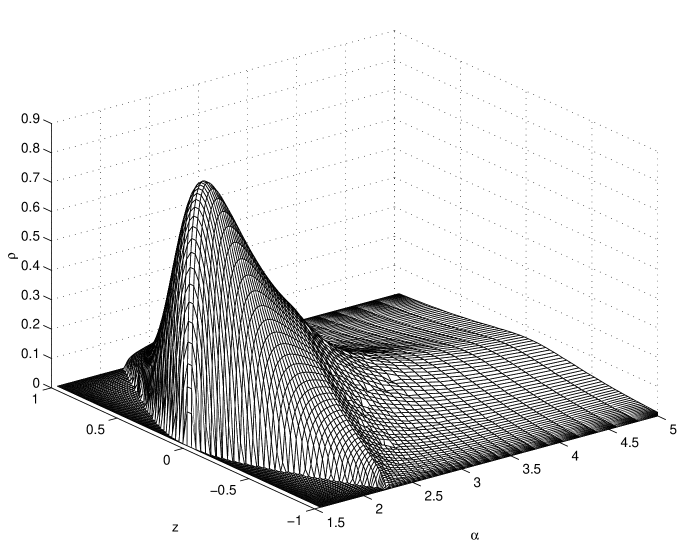
Figure 6: The re-scaled weight function $\tilde{\rho}(\alpha,z)$ of the bound-state vertex for $\eta=0.95$ calculated in bare ladder approximation. The mass of the exchanged boson $m_{3}=0.5m$.

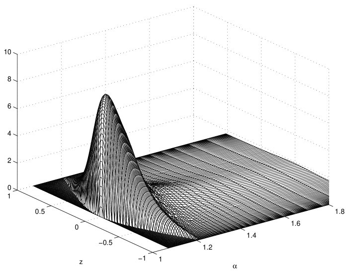
Figure 7: The same as in previous figure, but for $m_{3}=0.1m$ and $\eta=0.95$.

Where the independent numbers were available TJON , they agree with our results (see Table 3). If the mass of exchanged particle becomes small (but nonzero) the convergence of our numerical procedure becomes somewhat poorer and more sensitive to the initial guess. For illustration the weight functions $\tilde{\rho}^{[2]}$ is plotted in figs.(6,7) for two different values of exchanged mass.

V.2 Dressed Ladder BSE

In this subsection we finally discuss numerical solutions of the BSE including the dressing of the propagators. We introduce the dressing by two steps, switching it on first only for the exchanged particle and in the second step also for constituents. We should point out that since the solution of the DSEs in the bare vertex approximation (by which we dress the propagators) breaks down for coupling constants larger that $\tilde{\lambda}_{crit}=1.5$ we can consider to only rather weakly bound states: for the bare BSE $\tilde{\lambda}=1.5$ corresponds to $\eta=\sqrt{P^{2}}/(2m)\simeq 0.78$.

The propagator dressing of the exchanged particle in the one loop approximation was already considered in the Ref. KUSAK3 . We go beyond the one loop approximation and determine the continuum part of Lehmann weight $\sigma_{3}$ from the DSE (21) with the same value of the coupling constant. That is, we insert into Eq. (9 ) the dressed kernel

$$G_{3}(p-q)=\int_{0}^{\infty}d\omega\frac{\tilde{\sigma}_{3}(\omega)}{(p-q)^{2}-\omega+i\epsilon}$$ (28)

with the pole situated at $m_{3}=m/2$. As noted above, the constituent propagators are at this stage left undressed in the BSE, although they all self-energies have been taken fully into account in DSEs. The integration over $\omega$ (28) in the BSE kernel was performed using Gaussian quadrature with 16 points. Including the kernel self energy slightly decreases (by at most few per cent) the mass of the bound state, even for $\tilde{\lambda}\simeq\tilde{\lambda}_{crit.}$.

Let us point out, that the kernel of Eq. (9) in the dressed ladder kernel approximation is free of any singularities. The accuracy of the numerical solution is comparable to the the bare ladder case. For example, we $\tilde{\lambda}=0.734$ for $\eta=0.95$ for the grid of $32*32$ points and $\lambda=0.749(0.752)$ for the grid of $64*64(96*96)$, the convergence is similar to to the case of bare ladder (see the Tab.1). The extrapolated (to very large grid) values of $\lambda^{\prime}s$ for fractional binding $\eta=0.999,0.99,0.97,0.95$ are showed in Fig.8.

In the next step we have included the self energies of the constituents. As we shall see the effect is relatively small for $\tilde{\lambda}<<\tilde{\lambda}_{crit}$, but increases rapidly as $\tilde{\lambda}\rightarrow 1$. As in the previous case the Lehmann weights have been calculated from the DSEs solved for the same value of the coupling. As the first guess we have used the solution of the BSE linearized in $\tilde{\sigma}(\alpha)$, i.e. with only one propagator dressed. This guess is rather close to the exact solution for $\eta\leq 0.9$.

The constituent particle in a weakly bound system ($\eta\simeq 1$) live near their mass shell. Therefore, one can naively assume that the values of coupling for such weakly bound state should not be strongly affected by dressing of constituent propagators. For deeper bound states we have found that the effect of the dressing of constituents is much larger than that due to the dressing of the kernel (exchanged particle) Fig.8. The couplings for fully dressed BSE are not determined with the same high accuracy as those for the bare ladder BSE, since the grids are not optimalized for very different ratios of $\alpha$’s which appear in the kernel of the BSE.

V.3 Charge form factor

Various form factors are extensively studied in scalar theories like Wick-Cutkosky model (see for example AMGHAR ). In these studies the dependence of the form factor on the binding and on the range of the “strong” interaction has been considered, therefore we perform a similar calculations in our formalism.

In the approach adopted in this paper (employing the spectral representations in the Minkowski space), the bound states masses and corresponding vertex functions can be obtained with good accuracy and in reasonable CPU time. Unfortunately, the calculation of the scalar form factor as outlined in appendix B leads to more complicated results (68,69). Even if one would be able to perform analytically all additional Feynman integrations, the formula (69) still involves the four-dimensional integration over the spectral variables. We are taking also the integrals over four Feynman variables numerically with the help of Gauss-Legendre quadrature, taking the number of points for each of them equal to the one for spectral variable $z$. Since relatively small number of integration points (from 16 to 40) was taken for each integration, the presented results have to be viewed rather as an estimate of form factor behavior. One can always refine the grids at the expense of longer CPU time.

We have also compared our results to choose obtained in the Gross (spectator) formalism, choosing the ”scalar deuteron” parameters (see ORDEN ). In analogy with the real deuteron, the parameters are chosen as: $m_{3}/m=138/938.9,\eta=(2*938.9-2.3)/2*938.9\simeq 0.9988$. The bound state vertex functions were found by solution of the Gross and BS equations. All phenomenological form factors introduced in ORDEN have been ”switched off” (the limit $\Lambda^{\prime}s\rightarrow\infty$ are taken in the “strong” form factors) when calculating the Gross wave function and the bound state current. The e.m form factors were calculated in the spectator RIA and as described in appendix B (using the grid $32^{8}$), respectively.

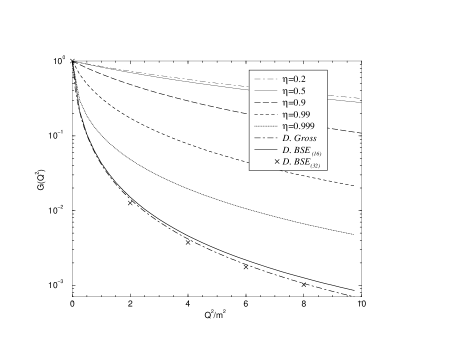
Figure 9: The behavior of the elastic electromagnetic form factors for various bound states characterized by $\eta$. The mass of exchanged particle is fixed to be $m_{3}=0.5m$, except for the scalar deuteron case (D.), which is calculated for comparison using two different grids.

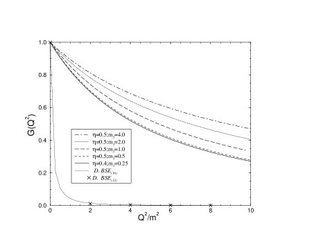
Figure 10: Variation of the elastic electromagnetic form factors with the mass of the exchanged particle while $\eta=0.5$ is fixed. The cases $\eta=0.4$, $m_{3}=0.25m$ and the scalar deuteron are included for comparison.

The form factors for several bound states listed in the Tables 1 and 3 are presented in Figs.9 and 10, respectively. In Fig.9 the ratio of the exchanged and constituent mass is kept constant $m_{3}/m=0.5$ and the mass of the bound state $M=\sqrt{P^{2}}$ is varied. In agreement with physical expectations one sees that as the bound state become more tight the elastic form factor increases. (For the infinitely bound point system is should be equal to unity, even our deepest bound state are of course still only approaching this value.) We put into the same plot for comparison also the scalar deuteron result. How the form factror changes with the mass of the exchanged particle is shown in Fig.10. We included several states for which $M=m$, bound by the one-boson-exchange potential of the range $r=1/m_{3}$, which is varied. Two other systems, first with $\eta=0.4;m_{3}=0.25$ and the scalar deuteron, are added for comparison. From both figure we can conclude that the behavior of form factor is determined by the strength of the interaction and its range rather differently for various $M$. The range of the interaction is more significant for a weaker ones. This agrees with conclusions of ref. THEUSL , which have also compared our results for small exchanged mass $\eta=0.8,m_{3}=0.15m$ with Wick-Cutkosky model prediction for $\eta=0.784,m_{3}=0$ (Tables 2 and 1 of THEUSL , respectively), and found only slight difference in the range $Q^{2}=(0,100m^{2})$.

VI Concluding Remarks

The spectral representation was employed for solving the Bethe-Salpeter equation in (3+1) Minkowski space. The new analytical formula for the integral equation kernel has been derived.

The method is efficient solving both the bare and dressed ladder BSE. Solution of Dyson-Schwinger equations for propagators leads to appearance of critical value of the coupling constant, beyond which the solution collapses. This restricts substantially the region in which the effects of dressing can be studied. Since the coupling is rather weak, the dressing leads only to moderate decrease of the bound state masses: even close to the critical value of the coupling the fractional binding of the bound state of the dressed BSE is smaller than the corresponding one for the bare BSE by at most 15 per cents. As an example of application of the obtained vertex functions, we calculated the elastic electromagnetic form factor.

To further develop the method, it would be interesting to extend it to more complicated BS kernel: trying to include the cross boxed contributions, $s$ and $u$ channel interactions etc. It is already known that the “spectral” approach used here is suitable even for more complicated systems, for scalar QED see Ref. FULTON . One of our future goals is to manage the complication due to fermionic degrees of freedom.

Appendix A Kernel Functions

In this appendix the real integral equation for the BS vertex weight is derived in detail. The PTIR form for scalar bound-state vertex reads

$$\Gamma(p,P)=\int\limits_{-1}^{1}dz\,\int\limits_{\alpha_{min}(z)}^{\infty}d\alpha\,\,\frac{\rho^{[n]}(\alpha,z)}{[F(\alpha,z;p,P)]^{n}}\quad,$$ (29)

where $\rho^{[n]}(\alpha,z)$ is the real PTIR weight function for the bound state vertex function, and $n$ is a dummy parameter. The function $F$ is given by NAKANATO

$$F(\alpha,z;p,P)=\alpha-(p^{2}+zp\cdot P+P^{2}/4)-i\epsilon=\alpha-f(p,P,z)-i\epsilon\quad.$$ (30)

The support of $\rho^{[n]}(\alpha,z)$ can be determined in general (see NAKANATO ) for arbitrary interaction. In our case of one-boson-exchange interaction kernel one gets a bit higher $\alpha_{min}$ KUSAK3 . We discuss our treatment of the lower bounds below.

The following procedure is straightforward but a bit exhaustive. The rhs of the BSE (4) with the kernel given by the exchange of the single (dressed) particle $\Phi_{3}$ has to be re-written in the form allowing to extract the integral equation for the spectral function $\rho^{[n]}(\alpha,z)$. The integrand contains the two “constituent” propagators, the denominator $F(\alpha,z,k,P)$ from the spectral representation of $\Gamma(k,P)$ and the propagator of the exchanged particle (all other factors will be skipped for a while for the sake of briefness).

Using the Feynman parameterization technique we first write

$$D(k+P/2;\alpha_{1})D(-k+P/2;\alpha_{2})=\frac{1}{2}\int\limits_{-1}^{1}\frac{d\eta}{[M^{2}-f(k,P,\eta)-i\epsilon]^{2}}\,,$$

$$M^{2}(\eta)=\frac{\alpha_{1}+\alpha_{2}}{2}+\frac{\alpha_{1}-\alpha_{2}}{2}\,\eta\,.$$ (31)

Next the denominator of (29) is added:

$$\frac{D(k+P/2;\alpha_{1})D(-k+P/2;\alpha_{2})}{[F(\alpha,z;k,P)]^{n}}=\frac{\Gamma(n+2)}{2\Gamma(n)}\,\int\limits_{-1}^{1}d\eta\int\limits_{0}^{1}dt\frac{(1-t)t^{n-1}}{[R-f(k,P,z^{\prime})-i\epsilon]^{n+2}}\,,$$

$$R=\alpha t+(1-t)M^{2}\,,$$ (32)

where $z^{\prime}=tz+(1-t)\eta$. Now, we include the propagator of the exchanged particle, the integral over $d^{4}k$ and factors $ig^{2}$, defining:

$$I_{DDDF}=ig^{2}\,\int\frac{d^{4}k}{(2\pi)^{4}}\frac{D(k+P/2;\alpha_{1})D(-k+P/2;\alpha_{2})D(p-k;\alpha_{3})}{[F(\alpha,z,p,P)]^{n}}$$ (33)

$$\hskip 56.9055pt=-ig^{2}\,\frac{\Gamma(n+3)}{2\Gamma(n)}\,\int\limits_{-1}^{1}d\eta\int\limits_{0}^{1}dt\,(1-t)t^{n-1}\int\limits_{0}^{1}dx\,x^{n+1}\,I_{k}\,,$$

$$I_{k}=\int\frac{d^{4}k}{(2\pi)^{4}}\left[-k^{2}+2k\cdot Q-(1-x)p^{2}-\frac{x}{4}P^{2}+(1-x)\alpha_{3}+xR-i\epsilon\right]^{-(n+3)}$$

$$\hskip 56.9055pt=\frac{i}{(4\pi)^{2}}\frac{\Gamma(n+1)}{\Gamma(n+3)}\frac{1}{x^{n+1}(1-x)^{n+1}}\,\frac{1}{[A-f(k,P,z^{\prime})-i\epsilon]^{n+1}}$$

$$A=\frac{R}{1-x}+\frac{\alpha_{3}}{x}-\frac{x}{(1-x)}\,S\,,$$ (34)

where $Q=(1-x)p-xz^{\prime}P/2$ and $S=\frac{1-z^{\prime 2}}{4}P^{2}$. Since $z^{\prime}$ lies in the interval $<-1,+1>$, $0\leq S<(m_{1}+m_{2})^{2}/4$. Interchanging the integrals over $\eta$ and $t$ with the help of:

$$\int\limits_{-1}^{1}d\eta\int\limits_{0}^{1}dt=\int\limits_{-1}^{1}dz^{\prime}\left[\int_{0}^{T_{+}}\frac{dt}{1-t}\,\Theta(z-z^{\prime})+\int_{0}^{T_{-}}\frac{dt}{1-t}\,\Theta(z^{\prime}-z)\right]\,,$$

$$T_{\pm}=\frac{1\pm z^{\prime}}{1\pm z}\quad\quad\mbox{and}\quad\quad z^{\prime}=tz+(1-t)\eta\,,$$ (35)

and introducing $\lambda=g^{2}/(4\pi)^{2}$ we get

$$I_{DDDF}=\lambda\,\frac{n}{2}\int\limits_{-1}^{1}dz^{\prime}\int\limits_{0}^{1}\frac{dx}{(1-x)^{n+1}}\sum_{s=\pm}\Theta(s(z-z^{\prime}))\int\limits_{0}^{T_{s}}\frac{dt\,t^{n-1}}{[F(A,z^{\prime},p,P)]^{n+1}}\,,$$ (36)

Let us separate the $t$ dependence of $F(A,z^{\prime};p,P)$. First we substitute for $\eta$ into the definition of $M^{2}$, which yields

$$(1-t)M^{2}=-t\left(\frac{\alpha_{1}+\alpha_{2}}{2}+\frac{\alpha_{1}-\alpha_{2}}{2}z\right)+\frac{\alpha_{1}+\alpha_{2}}{2}+\frac{\alpha_{1}-\alpha_{2}}{2}\,z^{\prime}\,.$$

Next, we introduce the notation (indicating explicitly the $t$-dependence of $A$ and $R$):

$$A(t)\equiv\frac{R(t)}{1-x}+\frac{\alpha_{3}}{x}-\frac{x}{1-x}\,S=\frac{R(t)-S}{1-x}+\frac{\alpha_{3}}{x}+S\,,$$ (37)

$$R(t)\equiv\alpha t+(1-t)M^{2}=J(\alpha,z)t+\frac{\alpha_{1}+\alpha_{2}}{2}+\frac{\alpha_{1}-\alpha_{2}}{2}\,z^{\prime}$$ (38)

$$J(\alpha,z)\equiv\ \alpha-\frac{\alpha_{1}+\alpha_{2}}{2}-\frac{\alpha_{1}-\alpha_{2}}{2}\,z\,,$$ (39)

in which the $t-$dependence of $F(A(t),z^{\prime},p,P)$ reads

$$F(A(t),z^{\prime};p,P)=\frac{J(\alpha,z)}{1-x}\,t+F(A(0),z^{\prime};p,P)\,.$$

Since t-dependence of $F(A(t),z^{\prime};p,P)$ is linear, the integral over $t$ can be taken:

$$\int\frac{dt\,t^{n-1}}{F(A(t),z^{\prime};p,P)^{n+1}}=\frac{t^{n}}{n\,F(A(0),z^{\prime};p,P)\,[F(A(t),z^{\prime};p,P)]^{n}}\,.$$

and hence

$$I_{DDDF}=\frac{\lambda}{2}\,\int\limits_{-1}^{1}dz^{\prime}\int\limits_{0}^{1}\frac{dx}{(1-x)^{n+1}}\sum_{s=\pm}\frac{\Theta(s(z-z^{\prime}))\,T_{s}^{n}}{F(A(0),z^{\prime};p,P)\,[F(A(T_{s}),z^{\prime};p,P)]^{n}}\,.$$ (40)

Using this result, the BSE can be written as follows:

$$\int\limits_{-1}^{1}dz^{\prime}\,\int\limits_{\alpha_{min}(z^{\prime})}^{\infty}d\alpha^{\prime}\,\,\frac{\rho^{[n]}(\alpha^{\prime},z^{\prime})}{[F(\alpha^{\prime},z^{\prime},p,P)]^{n}}=\left[\int\limits\sigma\right]^{3}\int d\alpha\int dz\rho^{[n]}(\alpha,z)\,I_{DDDF}\,.\,$$ (41)

$$\left[\int\limits\sigma\right]^{3}\equiv\int\limits_{\alpha_{1,min}}^{\infty}d\alpha_{1}\,\tilde{\sigma}_{1}(\alpha_{1})\int\limits_{\alpha_{2,min}}^{\infty}d\alpha_{2}\,\tilde{\sigma}_{2}(\alpha_{2})\int\limits_{\alpha_{3,min}}^{\infty}d\alpha_{3}\,\tilde{\sigma}_{3}(\alpha_{3})\,,$$ (42)

where $\tilde{\sigma}({\alpha_{i}})$ are the Lehmann functions of the dressed propagators, reducing to the $\delta$-function if the dressing is neglected. Obviously, the rhs is still not quite in the desired form, both $F(A(0),z^{\prime},p,P)$ and $F(A(T_{s}),z^{\prime},p,P)^{n}$ are functions of momenta $p$ and $P$.

Below we re-write the kernel as a sum of several fractions, which after substitution $\alpha^{\prime}=A(T),T=0,T_{\pm}$ would allow to use the uniqueness theorem NAKANATO and extract the BSE in the spectral form. This is possible only if the integrals over $\alpha^{\prime}$ on both right and left hand sides of 41 are taken over the same intervals. To show this it is first necessary to prove that $R(T)-S>0$, for $T=0,T_{\pm}$, since the functions $A(T)\rightarrow+\infty$ for $x\rightarrow 0$ and $x\rightarrow 1$ they have on for $0<x<1$ the minimum equal to:

$$A_{min}(T)=\left(\sqrt{R(T)-S}+m_{3}\right)^{2}+S=R(T)+m^{2}_{3}+2m_{3}\,\sqrt{(R(T)-S)}\,.$$ (43)

next, one has to show that these lower bounds are not in conflict with the lower bound for $\alpha^{\prime}$ (and the same lower bound for $\alpha$). It is simple for the undressed equal mass case, when the condition above taken for $T=0$ actually defines the lower bound for $\alpha$ in the following form

$$\alpha\geq\left(\sqrt{m^{2}-S(z^{\prime})}+m_{3}\right)^{2}+S(z^{\prime})\,,$$ (44)

and the same for $\alpha,z\rightarrow\alpha^{\prime},z^{\prime}$. Since $R(T_{\pm})$ depend also on $\alpha$ and $z$ and since for the equal mass case $R(T_{\pm})\geq R(0)$, the next two constrains clearly conform with the lower bound for $\alpha^{\prime}$ and one can extract from them the upper bound for the integration over $\alpha$:

$$\alpha\leq m^{2}+\frac{1}{T_{\pm}}\,\left[\left(\sqrt{\alpha^{\prime}-S(z^{\prime})}-m_{3}\right)^{2}+S(z^{\prime})-m^{2}\right]\,,$$ (45)

(compare to eq.(A6) of KUSAK3 , where one bracket seems to be misplaced). For the unequal mass case or for the dressed propagators this analysis is much more complicated, mostly due to the fact that now for some combination of parameters it can occur $R(T_{\pm})<R(0)$. The necessary condition $R(T)-S>0$ can again be proven in this case (though after much longer algebra), ensuring that the common lower bound for $\alpha$’s exists. But we could not resolve the conditions (43) analytically, they are treated numerically.

Now, let so go back to eq. (41) and proceed by considering first the simple case of the symmetric Wick-Cutkosky model.

A.1 The Wick-Cutkosky Model

In this model the constituents have the same masses $m_{1}=m_{2}=m$ and the mass of the exchanged particle is zero (all propagator dressings are neglected). Then for the S-wave ground state vertex function, the spectral function depends only on variable $z$ and the denominator enters with power $n=1$ (8):

$$\rho^{[n]}(\alpha,z)\rightarrow\delta(\alpha-m^{2})\rho(z)\,,$$ (46)

and in $I_{DDDF}$ we replace

$$n\rightarrow 1\,,\quad\quad M^{2}\rightarrow m^{2}\,,\quad\quad R(t)\rightarrow m^{2}\,,\quad\quad J(\alpha,z)\rightarrow 0\,,$$

$$A(t)\rightarrow A=\frac{m^{2}}{1-x}-\frac{x}{1-x}\,S\,,$$

$$I_{DDDF}\rightarrow\frac{\lambda}{2}\,\int\limits_{-1}^{1}dz^{\prime}\sum_{s=\pm}\Theta(s(z-z^{\prime}))\,T_{s}\,\int_{0}^{1}\frac{dx}{[m^{2}-xS-(1-x)f(p,P,z^{\prime})-i\epsilon]^{2}}\,.$$

Taking the integral over $x$ we find (recall that for equal masses $0\leq S<m^{2}$):

$$I_{DDDF}\rightarrow\frac{\lambda}{2}\,\int\limits_{-1}^{1}dz^{\prime}\sum_{s=\pm}\frac{\Theta(s(z-z^{\prime}))\,T_{s}}{m^{2}-S}\,\frac{1}{m^{2}+f(p,P,z^{\prime})-i\epsilon}\,.$$

Comparing both sides of the BSE and using the uniqueness theorem NAKANATO , we get the well-known (see e.g. Nakan ) integral equation for $\rho^{[1]}(z)$:

$$\rho(z^{\prime}) = \lambda\int\limits_{-1}^{1}dzV^{[1]}(z^{\prime},z)\,\rho(z)\,,$$ (47)

$$V^{[1]}(z^{\prime},z) = \sum_{s=\pm}\,\frac{\Theta(s(z-z^{\prime}))\,T_{s}}{2(m^{2}-S)}\,.$$

Although its solution is known analytically even for exited states, the energy spectrum still has to be found numerically (up to the $P^{2}=0$ corresponding to $\lambda=2$). For the purpose of numerical treatment, this equation is usually rewritten in the form:

$$\frac{\rho(z^{\prime})}{\lambda} = V_{0}(z^{\prime})-\int\limits_{-1}^{1}dz\rho(z)V_{\pm}(z^{\prime},z)$$

$$V_{0}(z^{\prime})=\frac{1}{2(m^{2}-S)}\quad \quad V_{\pm}(z^{\prime},z)=\frac{\frac{z^{\prime}-z}{1-z}\Theta(z^{\prime}-z)+\frac{z-z^{\prime}}{1+z}\Theta(z-z^{\prime})}{2(m^{2}-S)}\,\,$$ ;

where the temporary auxiliary normalization condition $\int dz\rho(z)=1$ was imposed (i.e., if used in further application, the vertex function would have to be re-normalized in accordance to (5)).

A.2 The BSE for $n=1$

We will now bring eqs. (40,41) to the desired form for the particular choice $n=1$. For the numerical solution this value is not the most suitable one. But since the formal manipulations are in this case the simplest, we treat it first for methodical reasons.

For $n=1$ the integrand of (40) can be decomposed into the sum of simpler fractions with the help of

$$\sum_{s=\pm}\frac{\Theta(s(z-z^{\prime}))\,T_{s}}{F(A(0),z^{\prime};p,P)\,F(A(T_{s}),z^{\prime};p,P)}=\frac{1-x}{J(\alpha,z)}\,\sum_{T}\frac{1}{F(A(T),z^{\prime};p,P)}\,,$$ (48)

where we have introduced a shorthand notation

$$\sum_{T}f(T)=f(0)-\theta(z-z^{\prime})f(T_{+})-\theta(z^{\prime}-z)f(T_{-})\,.$$ (49)

Notice that the lhs of (48) is nonsingular for $J(\alpha,z)=0$, so when this happens the rhs behaves like $0/0$, which calls for some caution in the numerics. So, the integral $I_{DDDF}$ now reads

$$I_{DDDF}(n=1)=\frac{\lambda}{2J(\alpha,z)}\,\sum_{T}\int\limits_{0}^{1}\frac{dx}{(1-x)F(A(T),z^{\prime};p,P)}\,.$$ (50)

In the last step we introduce the spectral variable $\alpha^{\prime}=A(T)$ and use the dependence of $A(T)$ on $x$ to convert the integration over $x$ into integral over $\alpha^{\prime}$. Picking up explicitly the $x$-dependence of $A(T)$ we can write:

$$g(x) \equiv A(T)=\frac{R(T)-S}{1-x}+\frac{\alpha_{3}}{x}+S\,,$$

$$g^{\prime}(x) = \frac{R(T)-S}{(1-x)^{2}}-\frac{\alpha_{3}}{x^{2}}=\frac{1}{1-x}\left(A-\frac{\alpha_{3}}{x^{2}}-S\right)\,,$$

$$\delta(\alpha^{\prime}-g(x)) = \sum_{i=\pm}\frac{1}{|g^{\prime}(x_{i})|}\,\delta(x-x_{i})\,,\quad\quad g(x_{\pm})=\alpha^{\prime}\,,$$

$$x_{\pm}(T) = \frac{\alpha^{\prime}-\alpha_{3}-R(T)\pm\sqrt{D}}{2(\alpha^{\prime}_{S})}\,,\quad D=(R(T)-\alpha^{\prime}+\alpha_{3})^{2}-4\alpha_{3}(R(T)-S)\,.$$

$$g^{\prime}(x_{\pm}) = \left(g(x_{\pm})-\frac{\alpha_{3}}{x_{\pm}^{2}}-S\right)\frac{1}{1-x_{\pm}}=\frac{E(x_{\pm},S,\alpha^{\prime})}{1-x_{\pm}}\,,$$

$$E(x_{\pm},S,\alpha^{\prime}) = \alpha^{\prime}-\frac{\alpha_{3}}{x_{\pm}^{2}}-S\,.$$ (51)

With the help of these relations we get

$$\sum_{T}\int\limits_{0}^{1}\frac{dx}{(1-x)F(A(T),z^{\prime};p,P)}=\int\limits_{\alpha_{min}^{\infty}}\frac{d\alpha^{\prime}}{F(\alpha^{\prime},z^{\prime};p,P)}\,\sum_{T}\,\sum_{i=\pm}\frac{\theta(x_{i}(T))\theta(1-x_{i}(T))\theta(D)}{|E(x_{i}(T),S,\alpha^{\prime})|}\,.$$

Using this result in (41), one gets from the uniqueness theorem the integral equation for the BSE structure function is obtained:

$$\rho^{[1]}(\alpha^{\prime},z^{\prime}) = \lambda\,\left[\int\limits\sigma\right]^{3}\int dz\int d\alpha\,V^{(1)}(\alpha,z,\alpha^{\prime},z^{\prime})\,\rho^{[1]}(\alpha,z)\,,$$ (52)

$$V^{(1)}(\alpha,z,\alpha^{\prime},z^{\prime}) = \frac{1}{2J(\alpha,z)}\,\sum_{T}\,\sum_{i=\pm}\frac{\theta(x_{i}(T))\theta(1-x_{i}(T))\theta(D)}{|E(x_{\pm}(T),S,\alpha^{\prime})|}\,.$$ (53)

Notice, that $x_{\pm}(T)$ depend on $\alpha^{\prime},z^{\prime}$ (which are fixed from the lhs), $\alpha_{1},\alpha_{2},\alpha_{3}$ (which are fixed when the dressing is neglected), $P^{2}$ in $S$ (which is given by the binding energy of the system) and for $T\neq 0$ also on $\alpha,z$ (through $J(\alpha,z)$ in $R(T_{\pm})$). This allows to recast the integral equation into the form more convenient for numerical treatment.

A.2.1 BSE without propagator dressing (for $n=1$)

If the propagator dressing is omitted, $\alpha_{i}\rightarrow m_{i}^{2}$ and the corresponding BSE for the spectral function reads

$$\rho^{[1]}(\alpha^{\prime},z^{\prime}) = \lambda\,\int dz\int d\alpha\,V^{[1]}(\alpha^{\prime},z^{\prime},\alpha,z)\rho^{[1]}(\alpha,z)\,,$$

$$V^{[1]}(\alpha^{\prime},z^{\prime},\alpha,z) = \frac{1}{2J(\alpha,z)}\,\sum_{T}\,\sum_{i=\pm}\frac{\theta(x_{i}(T))\theta(1-x_{i}(T))\theta(D)}{|E(x_{i}(T),S,\alpha^{\prime})|}$$

As mentioned above, for $T=0$ the kernel depends on $\alpha$ and $z$ only through $J(\alpha,z)$, hence it is convenient to pick up this case from the sum over $T$ and re-scaling

$$\rho^{[1]}(\alpha,z) = J(\alpha,z)\,\tilde{\rho}^{[1]}(\alpha,z)\,,$$

$$V^{[1]}(\alpha^{\prime},z^{\prime},\alpha,z) = \frac{J(\alpha^{\prime},z^{\prime})}{J(\alpha,z)}\,\tilde{V}^{[1]}(\alpha^{\prime},z^{\prime},\alpha,z)\,,$$

and imposing the auxiliary normalization

$$\int dz\int\alpha\,\tilde{\rho}^{[1]}(\alpha,z)=1\,,$$

rewrite the BSE in the non-homogenous form:

$$\tilde{\rho}^{[1]}(\alpha^{\prime},z^{\prime}) = \lambda\,\tilde{V}_{0}^{[1]}(\alpha^{\prime},z^{\prime})-\lambda\,\int dz\int\alpha\,\sum_{s=\pm}\tilde{V}_{s}^{[1]}(\alpha^{\prime},z^{\prime},\alpha,z)\,\tilde{\rho}^{[1]}(\alpha,z)\,,$$ (54)

$$\tilde{V}_{0}^{[1]}(\alpha^{\prime},z^{\prime}) = \frac{1}{2J(\alpha^{\prime},z^{\prime})}\,\sum_{i=\pm}\left[\frac{\theta(x_{i}(T))\theta(1-x_{i}(T))\theta(D)}{|E(x_{\pm}(T),S,\alpha^{\prime})|}\right]_{T=0}\,,$$

$$\tilde{V}_{s}^{[1]}(\alpha^{\prime},z^{\prime},\alpha,z) = \frac{\theta(s(z-z^{\prime}))}{2J(\alpha^{\prime},z^{\prime})}\,\sum_{i=\pm}\left[\frac{\theta(x_{i}(T))\theta(1-x_{i}(T))\theta(D)}{|E(x_{\pm}(T),S,\alpha^{\prime})|}\right]_{T=T_{s}}\,.$$

The $\theta$ functions in the kernel impose the proper bounds on $\alpha$ and ensure that the rhs contributes only for $\alpha^{\prime}$ from the support of $\tilde{\rho}^{[1]}(\alpha^{\prime},z^{\prime})$.

A.3 BSE for $n=2$

Now, we would first describe the necessary modifications for the choice $n=2$ which was used in actual numerical calculations in this paper. Going back to (40) we can for this case write:

$$\sum_{s=\pm}\frac{\Theta(s(z-z^{\prime}))\,T_{s}^{2}}{F(A(0),z^{\prime},p,P)\,F(A(T_{s}),z^{\prime},p,P)^{2}}=$$

$$\hskip 85.35826pt\frac{1-x}{J(\alpha,z)}\,\sum_{T}\left[\frac{T}{[F(A(T),z^{\prime};p,P)]^{2}}+\frac{1-x}{J(\alpha,z)}\,\frac{1}{F(A(T),z^{\prime};p,P)}\right]\,.$$

Then, the integral $I_{DDDF}$ can be cast into form:

$$I_{DFFF} = \frac{\lambda}{2J(\alpha,z)}\,\int_{-1}^{1}dz^{\prime}\int_{0}^{1}\,\frac{dx}{(1-x)^{2}}\,\sum_{T}\left[\frac{T}{[F(A(T),z^{\prime};p,P)]^{2}}+\frac{1-x}{J(\alpha,z)}\,\frac{1}{F(A(T),z^{\prime};p,P)}\right]$$

$$= \frac{\lambda}{2J(\alpha,z)}\,\int_{-1}^{1}dz^{\prime}\sum_{T}\,\frac{dx}{[F(A(T),z^{\prime};p,P)]^{2}}\,\left[\frac{T}{(1-x)^{2}}-\frac{\ln{(1-x)}}{J(\alpha,z)}\frac{dA(T)}{dx}\right]$$

$$= \frac{\lambda}{2J(\alpha,z)}\,\int_{-1}^{1}dz^{\prime}\int_{\alpha_{min}}^{\infty}\frac{d\alpha^{\prime}}{[F(\alpha^{\prime},z^{\prime};p,P)]^{2}}\,\sum_{T}\,\sum_{i=\pm}\,\theta(x_{i})\theta(1-x_{i})\theta(D)$$

$$\hskip 56.9055pt\left[\frac{T}{(1-x_{i})|E(x_{i},S,\alpha^{\prime})|}-\frac{\mbox{sgn}(E(x_{i},S,\alpha^{\prime})\ln{(1-x_{i})}}{J(\alpha,z)}\right]\,,$$

where we have first integrated the second term of the sum over $T$ by parts (to increase the power of $F(A(T),z^{\prime};p,P)$, the boundary term vanishes when $x\rightarrow 0,1$) and then introduced the integration over $\alpha^{\prime}$ as in the previous section.

Now, we can use the uniqueness theorem of PTIR NAKANATO and identify the BS weight function on the right-hand side of BSE:

$$\rho^{[2]}(\alpha^{\prime},z^{\prime}) = \lambda\,\int\limits_{-1}^{1}dz\int\limits_{-\infty}^{\infty}d\alpha\,V^{[2]}(\alpha^{\prime},z^{\prime};\alpha,z)\rho^{[2]}(\alpha,z)\,,$$ (55)

$$V^{[2]}(\alpha^{\prime},z^{\prime};\alpha,z) = \left[\int\sigma\right]^{3}\sum_{T}\sum_{i=\pm}\frac{\theta(x_{i})\theta(1-x_{i})\theta(D)}{2J(\alpha,z)^{2}}$$ (56)

$$\hskip 14.22636pt\left\{\frac{TJ(\alpha,z)}{(1-x_{i})|E(x_{i},S,\alpha^{\prime})|}-\mbox{sgn}\left(E(x_{i},S,\alpha^{\prime})\right)\ln(1-x_{i})\right\}.$$

Before treating the general case with fully dressed propagator we consider in the next subsection the pure ladder BSE.

A.3.1 BSE without propagator dressing (for $n=2)$

In this case we can proceed in a way very similar to the undressed BSE for $n=1$, only with different re-scaling factor

$$\rho^{[2]}(\alpha,z) = J(\alpha,z)^{2}\,\tilde{\rho}^{[2]}(\alpha,z)\,,$$

$$V^{[2]}(\alpha^{\prime},z^{\prime},\alpha,z) = \frac{J(\alpha^{\prime},z^{\prime})^{2}}{J(\alpha,z)^{2}}\,\tilde{V}^{[2]}(\alpha^{\prime},z^{\prime},\alpha,z)\,.$$

Imposing the auxiliary normalization

$$\int dz\int\alpha\,\tilde{\rho}^{[2]}(\alpha,z)=1\,,$$

we can write

$$\tilde{\rho}^{[2]}(\alpha^{\prime},z^{\prime}) = \lambda\,\tilde{V}_{0}^{[2]}(\alpha^{\prime},z^{\prime})-\lambda\,\int dz\int\alpha\,\sum_{s=\pm}\tilde{V}_{s}^{[2]}(\alpha^{\prime},z^{\prime},\alpha,z)\,\tilde{\rho}^{[2]}(\alpha,z)\,,$$ (57)

$$\tilde{V}_{0}^{[2]}(\alpha^{\prime},z^{\prime}) = \left.-\sum_{i=\pm}\frac{\theta(x_{i})\theta(1-x_{i})\theta(D)}{2J(\alpha^{\prime},z^{\prime})^{2}}{\mbox{sgn}}\left(E(x_{i},S,\alpha^{\prime})\right)\ln(1-x_{i})\right|_{x_{i}=x_{i}(T=0)}\,$$

$$\tilde{V}_{s}^{[2]}(\alpha^{\prime},z^{\prime},\alpha,z) = \frac{\theta(s(z-z^{\prime}))}{2J(\alpha^{\prime},z^{\prime})^{2}}\,\sum_{i=\pm}\theta(x_{i})\theta(1-x_{i})\theta(D)\,$$

$$\hskip 14.22636pt\left\{\frac{T_{s}J(\alpha,z)}{(1-x_{i})|E(x_{i},S,\alpha^{\prime})|}-{\mbox{sgn}}\left(E(x_{i},S,\alpha^{\prime})\right)\ln(1-x_{i})\right\}_{x_{i}=x_{i}(T_{s})}\,.$$

A.3.2 Dressed ladder BSE for $n=2$

When the all self-energies are taken into account the function $J(\alpha,z)$ do not factorize and numerically convenient redefinition (A.3.1) can not be used. Nevertheless, we can still separate from the integral over spectral variables $\alpha_{i}$ and the sum over $T$ the term which depends on $\alpha$ and $z$ only through $J(\alpha,z)$, namely the part for which $\tilde{\sigma}_{i}\rightarrow\delta(\alpha_{i}-m_{i}^{2})$ and $T=0$. Explicitly, using the notation

$${\cal V}(\alpha^{\prime},z^{\prime},\alpha,z,T,\alpha_{1},\alpha_{2},\alpha_{3}) = \sum_{i=\pm}\frac{\theta(x_{i})\theta(1-x_{i})\theta(D)}{2J(\alpha,z)^{2}}\,$$

$$\left\{\frac{TJ(\alpha,z)}{(1-x_{i})|E(x_{i},S,\alpha^{\prime})|}-{\mbox{sgn}}\left(E(x_{i},S,\alpha^{\prime})\right)\ln(1-x_{i})\right\}_{x_{i}=x_{i}(T)}\,,$$

and imposing the normalization condition

$$1=\int\limits_{-1}^{1}dz\int\limits_{-\infty}^{\infty}d\alpha\frac{\rho^{[2]}(\alpha,z)}{J(\alpha,z)^{2}}\,,$$

the BSE can be re-written as

$$\rho^{[2]}(\alpha^{\prime},z^{\prime}) = \lambda\,V_{0}^{[2]}(\alpha^{\prime},z^{\prime})+\lambda\,\int dz\int d\alpha\,\sum_{T}V_{T}^{[2]}(\alpha^{\prime},z^{\prime},\alpha,z)\,\rho^{[2]}(\alpha,z)\,,$$

$$V_{0}^{[2]}(\alpha^{\prime},z^{\prime}) = -\frac{1}{2}\int d\alpha_{3}\,\tilde{\sigma}(\alpha_{3})\sum_{s=\pm}\sum_{i=\pm}\theta(x_{i})\theta(1-x_{i})\theta(D)\,{\mbox{sgn}}\left(E(x_{i},S,\alpha^{\prime})\right)\ln(1-x_{i})\,,$$

$$V_{T}^{[2]}(\alpha^{\prime},z^{\prime},\alpha,z) = \int d\alpha_{3}\,\tilde{\sigma}(\alpha_{3})\int d\alpha_{1}d\alpha_{2}\,$$

$$\left[\delta_{1}\delta_{2}(1-\delta_{T,0})+\delta_{1}\sigma_{2}+\sigma_{1}\delta_{2}+\sigma_{1}\sigma_{2}\right]\,{\cal V}(\alpha^{\prime},z^{\prime},\alpha,z,T,\alpha_{1},\alpha_{2},\alpha_{3})\,,$$

where in $V_{0}^{[2]}(\alpha^{\prime},z^{\prime})$ we take $x_{i}=x_{i}(T=0)$, $\alpha_{1}=m_{1}^{2}$, $\alpha_{2}=m_{2}^{2}$ and in the last term $\delta_{i}=\delta(\alpha_{i}-m_{i}^{2})$ and $\sigma_{i}=\sigma(\alpha_{i}-m_{i}^{2}),i=1,2$.

Appendix B Elastic Electromagnetic Form Factor

In this Appendix we derive the expression for the elastic electromagnetic form factor $G(Q^{2})$. The relevant matrix element is diagrammatically depicted in the Fig.4 and the starting equation for the e.m. matrix element is given by (26). The labeling of momenta corresponds to the Fig.4: $q$ is a virtual photon incoming momentum and we put $Q^{2}=-q^{2}>0$, $P_{i}=P$ and $P_{f}=P+q$ are the total momenta of bound state in in- and out-state, respectively. For simplicity, we will consider the equal mass case: $m_{1}^{2}=m_{2}^{2}=m^{2}$.

The form factor $G(Q^{2})$ can easily be extracted from its definition (25). After multiplying by $P_{i}+P_{f}$ we get

$$G(Q^{2})=\frac{G_{\mu}(P+q,P)(2P+q)^{\mu}}{e(2P+q)^{2}}\quad,$$ (58)

The matrix element is evaluated between on-shell states of appropriate composite scalar, i.e. $P^{2}=(P+q)^{2}=M^{2}$ which implies

$$2P.q+q^{2}=0$$ (59)

The one body current $j_{\mu}$ reads

$$j^{\mu}(p_{f},p_{i})=(P+2k+q)^{\mu}\quad.$$ (60)

Using (59) one can simplify

$$(2P+q)^{2} = 4M^{2}+Q^{2}\,,$$

$$(2P+q)\cdot((2k+q+P) = 2k\cdot(2P+q)+2M^{2}+\frac{Q^{2}}{2}\,$$

$$\frac{(2P+q)\cdot((2k+q+P)}{(2P+q)^{2}} = \frac{1}{2}\left(1+\frac{4k\cdot(2P+q)}{4M^{2}+Q^{2}}\right)\,.$$

Taking this into account we can write:

$$G(Q^{2}) = \frac{i}{2}\,\int\frac{d^{4}k}{(2\pi)^{4}2}\,\left(\prod_{i=1}^{3}D_{i}\right)\,\left(\bar{\Gamma}\Gamma\right)\,\left[1+\frac{4k\cdot(2P+q)}{4M^{2}+Q^{2}}\right]\quad,$$ (61)

$$\prod_{i=1}^{3}D_{i} = D(k+\frac{P}{2};m^{2})D(-k+\frac{P}{2};m^{2})D(k+q+\frac{P}{2};m^{2})\,\,,$$ (62)

$$\bar{\Gamma}\Gamma = \bar{\Gamma}(k+\frac{q}{2},P+q)\Gamma(k,P)\,.$$ (63)

Now, we will express $G(Q^{2})$ in terms of spectral functions of the bound state vertex functions $\Gamma$, re-writing first the product of the propagators with the help of the Feynman parametrization.

For the product of the propagators one gets:

$$\prod_{i=1}^{3}D_{i} = D(k+q+\frac{P}{2})\,\,\frac{1}{2}\int\limits_{-1}^{1}d\eta\frac{1}{\left[k^{2}+\eta k\cdot P+\frac{P^{2}}{4}-m^{2}+i\epsilon\right]^{2}}$$ (64)

$$= \int\limits_{0}^{1}ds\int\limits_{2s-1}^{1}dy\frac{1}{[k^{2}+\frac{M^{2}}{4}-m^{2}-\frac{s}{2}Q^{2}+2sk\cdot q+yk\cdot P+i\epsilon]^{3}}$$

where the substitution $y=s+(1-s)\eta$ has been used and relations $P\cdot q=Q^{2}/2$ and $P^{2}=M^{2}$ has been replaced used.

Next step we combine PTIR (for $n=2$) of the product of the bound state vertex functions.

$$\int\limits_{0}^{\infty}d\alpha_{1}d\alpha_{2}\int\limits_{-1}^{1}dz_{1}dz_{2}\rho^{[2]}(\alpha_{1},z_{1})\rho^{[2]}(\alpha_{2},z_{2})\left\{\int\limits_{0}^{1}dx\frac{\Gamma(4)}{\Gamma(2)\Gamma(2)}\frac{x(1-x)}{G^{4}}\right\}$$

$$G = k^{2}+\frac{M^{2}}{4}+(z_{1}+x(z_{2}-z_{1}))k\cdot P+x(1+z_{2})k\cdot q-x(1+z_{2})\frac{Q^{2}}{4}$$ (65)

$$-(1-x)\alpha_{1}-x\alpha_{2}+i\epsilon\,.$$

Making use of the Feynman variable $t$ for matching (64) with the term in large brackets of (B), the relation for the form factor (61) can be rewritten as

$$I(Q^{2}) = -\frac{i}{2}\frac{\Gamma(7)}{\Gamma(3)}\,\int\limits_{0}^{1}ds\int\limits_{2s-1}^{1}dy\int\limits_{0}^{1}dx\,x(1-x)\,\int\limits_{0}^{1}dt\,t^{3}(1-t)^{2}$$

$$\int\frac{d^{4}k}{(2\pi)^{4}}\,\frac{\left[1+4\frac{(2P+q).k}{(2P+q)^{2}}\right]}{\left[c-k^{2}-k\cdot(aP+bq)-i\epsilon\right]^{7}}$$

$$a = t[z_{1}+x(z_{2}-z_{1})]+(1-t)y\,,$$

$$b = tx(1+z_{2})t+2s(1-t)\,,$$

$$c = b\,\frac{Q^{2}}{4}-\frac{M^{2}}{4}+(1-t)m^{2}+t(1-x)\alpha_{1}+tx\alpha_{2}\,.$$ (66)

where we have omitted the vertex weight functions and the $\alpha,z$’s integrals (exactly the pre-factor in front of the large bracket in (B)). Integration over the momentum $k$ (with the shift $k+(aP+bq)/2\rightarrow k$ then yields

$$-\frac{i}{2}\,\frac{\Gamma(7)}{\Gamma(3)}\,\int\frac{d^{4}k}{(2\pi)^{4}}\,\frac{1+\frac{2k\cdot(2P+q)}{4M^{2}+Q^{2}}}{\left[c-k^{2}-k\cdot(aP+bq)-i\epsilon\right]^{7}}=\frac{\Gamma(5)}{4(4\pi)^{2}}\,\frac{1-\frac{4(Pa+qb).(2P+q)}{4M^{2}+Q^{2}}}{\left[c+\frac{1}{4}(Pa+qb)^{2}\right]^{5}}$$ (67)

This relation can be further simplified using (59) in both the numerator and the denominator

$$I(Q^{2}) = \frac{\Gamma(4)}{(4\pi)^{2}}\,\int\limits_{0}^{1}dt\int\limits_{0}^{1}dx\int\limits_{0}^{1}dy\int\limits_{0}^{\frac{1+y}{2}}ds\,\,\frac{x(1-x)t^{3}(1-t)^{2}(1-a)}{\left[\frac{Q^{2}}{4}b(b-a-1)-r\right]^{5}}$$ (68)

$$r = -(1-a^{2})\frac{M^{2}}{4}+(1-t)m^{2}+t(1-x)\alpha_{1}+tx\alpha_{2}\quad,$$

$$a = t[z_{1}+x(z_{2}-z_{1})]+(1-t)y\,,$$

$$b = tx(1+z_{2})t+2s(1-t)\,,$$

It can be shown that for $Q^{2}\geq 0$ the denominator is nonzero. The function $I(Q^{2})$ can be easily calculated numerically. Including the missing pre-factors the elastic electromagnetic form factor is given by:

$$G(Q^{2}) = \int_{0}^{\infty}d\alpha_{1}d\alpha_{2}\int_{-1}^{1}dz_{1}dz_{2}\,\rho^{[2]}(\alpha_{1},z_{1})\rho^{[2]}(\alpha_{2},z_{2})\,I(Q^{2})\quad.$$ (69)

TABLE 1. Dimensioneless coupling $\tilde{\lambda}=g^{2}/(4\pi m)^{2}$ as a function of fraction of binding $\eta=\sqrt{P^{2}}/2m$ for two cases of exchanged mass $m_{3}$. The case $m_{3}/m=0$ is the Wick-Cutkosky model. The second case $m_{3}/m=0.5$ is compared with the result obtained by Kusaka et al KUSAK3 .

TABLE 3. Dimensioneless coupling $\tilde{\lambda}=g^{2}/(4\pi m)^{2}$ for several selections of $m_{3}/m=$ and fraction of binding $\eta=\sqrt{P^{2}}/2m$, compared to the results of ref. TJON .

Figure 8: The eigenvalues $\tilde{\lambda}$ calculated for the bare BSE, with dressed kernel $V$ and for dressed ladder BSE. Beyond the critical value of coupling $\tilde{\lambda}_{crit}=1.5$ only the bare solution is available.

References

- (1) H. Bethe and E. Salpeter, Phys. Rev. 84,1232 (1951); Y. Nambu, Prog. Theor. Phys. 5, 614 (1950).
- (2) C.D. Roberts and A.G. Williams, Dyson-Schwinger Equations and their Application to Hadronic Physics, Prog. Part. Nuc. Phys. 33 (Pergamon Press, Oxford,) 1994.
- (3) R. Alkofer, L. von Smekal, Phys. Rep. 353, 281 (2001).
- (4) C.D. Roberts, S.M. Schmidt, Prog. Part. Nucl. Phys. 45S1, 103 (2000).
- (5) P. Maris and P.C. Tandy, Phys. Rev. C 62, 055204 (2000); (nucl-th/0005015).
- (6) N. Nakanishi, Suppl. Prog. Theor. Phys. 43, (1969).
- (7) N. Seto, Suppl. Prog. Theor. Phys. 95, 25 (1988).
- (8) K. Kusaka, K. Simpson , A.G. Williams, Phys. Rev. D 56, 5071 (1997).
- (9) S. Ahlig, R. Alkofer, Ann. Phys. 275, 113 (1999).
- (10) L. Theussl, B. Desplanques, Few Body Syst. 30, 5 (2001).
- (11) T. Nieuwenhuis and J.A. Tjon, Phys. Rev. Lett. 77, 814 (1996).
- (12) B. Desplanques, L. Theussl, Eur. Phys. J. A 13, 461 (2002); (nucl-th/0102060).
- (13) B. Ding, J. Darewych, J. Phys. G 26, 907 (2000).
- (14) J.R. Cooke and G.A. Miller, Phys. Rev. C 62, (2000); M. Mangin-Brinet and J. Carbonell, Phys. Lett. B 474, 237 (2000).
- (15) T. Nieuwenhuis and J.A. Tjon, Few Body Syst. 21,167 (1996).
- (16) G.C. Wick, Phys. Rev. 96, 1124 (1954).
- (17) K. Kusaka and A.G. Williams, Phys. Rev. D 51, 7026 (1995).
- (18) G. Feldman and T. Fulton, Phys. Rev. D 8, 3616 (1973).
- (19) N. Nakanishi, Graph Theory and Feynman Integrals, eds. Gordon and Breach, New York, 1971.
- (20) I. Fukui and N. Setoh, Prog. Theor. Phys. 95, 433 (1996) ; I. Fukui and N. Setoh, Prog. Theor. Phys. 101, 1335 (1999); (hep-ph/9901364).
- (21) V. Šauli, J. Adam , in preparation, preliminary version reported at XVIIth European Conference on Few-Body Physics, September 11-16, 2000, Evora, Portugal, Nuc. Phys. A 689, 467c (2001).
- (22) S. Mandelstam, Proc. Roy. Soc. A 233, 248 (1955).
- (23) A. Amghar, B. Desplanques, L. Theussl, nucl-th/0202046
- (24) J.W. Van Orden, Czech. J. Phys. 45, 181 (1995).
- (25) J. Adam, V. Šauli, in proceedings of 7th Conference, “Mesons and Light Nuclei ’98”, Prague-Pruhonice, Czech Republic, August 31–September 4, 1998, edts. J. Adam et al, World Scientific, 1998, p. 391; (hep-ph/0110090).