[ CERN-TH/2001-332 IFIC/01-65 hep-ph/0111432

On the Effect of $\theta_{13}$ on the Determination of Solar Oscillation Parameters at KamLAND

Abstract

If the solution to the solar neutrino puzzle falls in the LMA region, KamLAND should be able to measure with good precision the corresponding oscillation parameters after a few years of data taking. Assuming a positive signal, we study their expected sensitivity to the solar parameters ($\theta_{12}$,$\Delta m^{2}_{21}$) when considered in the framework of three–neutrino mixing after taking into account our ignorance on the mixing angle $\theta_{13}$. We find a simple “scaling” dependence of the reconstructed $\theta_{12}$ range with the value of $\theta_{13}$ while the $\Delta m^{2}_{12}$ range is practically unaffected. Our results show that the net effect is approximately equivalent to an uncertainty on the overall neutrino flux normalization of up to $\sim$ 10%.

]

The Sudbury Neutrino Observatory (SNO) measurement on the charged current reaction for solar neutrino absorption in deuterium [1] has provided an important piece of information in the path to solve the solar neutrino problem (SNP) [2, 3, 4, 5, 6]. In particular, all the post-SNO global analysis [7, 8, 9, 10, 11] have shown that the inclusion of the SNO results have further strengthen the case for solar neutrino oscillations with large mixing angles with best fit in the region with larger $\Delta m^{2}$, LMA. Unfortunately, the LMA region is broad in mixing and mass splitting due to the uncertainties in the solar fluxes and the lack of detailed data in the low energy range.

This situation will be improved in the very near future, in particular, if LMA is the right solution to the SNP. If Nature has arranged things favourably, the SNO measurements of the day-night asymmetry and the neutral to charged current ratio could help to identify and constrain the LMA solution [11]. Furthermore, the terrestrial experiment, KamLAND [12], should be able to identify the oscillation signal and significantly constrain the region of parameters for the LMA solution.

The KamLAND reactor neutrino experiment, which is to start taking data very soon, is sensitive to the LMA region of the solar neutrino parameter space. After a few years of data taking, it should be capable of either excluding the entire LMA region or, not only establishing $\nu_{e}\leftrightarrow\nu_{\rm other}$ oscillations, but also measuring the oscillation parameters $(\tan^{2}\theta_{12},\Delta m^{2}_{21})$ with unprecedented precision [13, 14, 15, 16, 17, 18]. Previous analysis of the attainable accuracy in the determination of the oscillation parameters at KamLAND have studied the effect of the time dependent fuel composition, the knowledge of the flux uncertainty, the role of the geological neutrinos as well as the combined analysis of solar and KamLAND data. These studies have been performed in the simplest two-neutrino oscillation scheme or equivalently for three-neutrino oscillations assuming a small fixed value of $\theta_{13}$ [13, 14, 15, 16, 17, 18].

In this letter, we revisit the problem of how the precision to which KamLAND should be able to measure the solar oscillation parameters, $\Delta m_{12}^{2}$ and $\theta_{12}$, is affected by our ignorance on the exact value of the mixing angle $\theta_{13}$. At present our most precise information on this parameter comes from the negative results from the CHOOZ reactor experiment [19], which, when combined with the results from the atmospheric neutrino experiments [20] results into a 3$\sigma$ upper bound $\sin^{2}\theta_{13}\lesssim 0.06$[21, 22]. To address this question we study how the reconstructed range of $\Delta m_{12}^{2}$ and $\theta_{12}$ depends on the value of the mixing angle $\theta_{13}$. We conclude that the reconstructed $\Delta m_{12}^{2}$ is very mildly affected by the value of $\theta_{13}$, while the $\theta_{12}$ range scales with $\theta_{13}$ in a simple way. We determine the reconstructed region of solar parameters obtained from a given signal once $\theta_{13}$ is left free to vary below the present bound. We find that the net effect is approximately equivalent to that of an uncertainty on the overall neutrino flux normalization of up to $\sim$ 10% and it should be taken into account once enough statistics is accumulated.

KamLAND is a reactor neutrino experiment located at the old Kamiokande site in the Kamioka mine in Japan. It is sensitive to the $\bar{\nu}_{e}$ flux from some 10+ reactors which are located “nearby.” The distances from the different reactors to the experimental site vary from slightly more than 80 km to over 800 km, while the majority (roughly 80%) of the neutrinos travel from 140 km to 215 km. KamLAND “sees” the antineutrinos by detecting the total energy deposited by recoil positrons, which are produced via $\bar{\nu}_{e}+p\rightarrow e^{+}+n$. The total visible energy corresponds to $E_{e^{+}}+m_{e}$, where $E_{e^{+}}$ is the total energy of the positron and $m_{e}$ the electron mass. The positron energy, on the other hand, is related to the incoming antineutrino energy $E_{e^{+}}=E_{\nu}-1.293$ MeV up to corrections related to the recoil momentum of the daughter neutron (1.293 MeV is the neutron–proton mass difference). KamLAND is expected to measure the visible energy with a resolution which is expected to be better than $\sigma(E)/E=10\%/\sqrt{E}$, for $E$ in MeV [12, 17].

The antineutrino spectrum which is to be measured at KamLAND depends on the power output and fuel composition of each reactor (both change slightly as a function of time), and on the cross section for $\bar{\nu}_{e}+p\rightarrow e^{+}+n$. For the results presented here we will follow the flux and the cross section calculations and the statistical procedure described in Ref. [18]. We use one “KamLAND-year” as the amount of time it takes KamLAND to see 800 events with visible energy above 1.22 MeV. This is roughly what is expected after one year of running (assuming a fiducial volume of 1 kton), if all reactors run at (constant) $78\%$ of their maximal power output [12]. We assume a constant chemical composition for the fuel of all reactors (explicitly, 53.8% of ²³⁵U, 32.8% of ²³⁹Pu, 7.8% of ²³⁸U, and 5.6% of ²⁴¹Pu, see [13, 23]).

The shape of the energy spectrum of the incoming neutrinos can be derived from a phenomenological parametrisation, obtained in [24],

$$\frac{{\rm d}N_{\bar{\nu}_{e}}}{{\rm d}E_{\nu}}\propto e^{a_{0}+a_{1}E_{\nu}+a_{2}E^{2}_{\nu}},$$ (1)

where the coefficients $a_{i}$ depend on the parent nucleus. The values of $a_{i}$ for the different isotopes we used are tabulated in [24, 16]. These expressions are very good approximations of the (measured) reactor flux for values of $E_{\nu}\gtrsim 2$ MeV.

The cross section for $\bar{\nu}_{e}+p\rightarrow e^{+}+n$ has been computed including corrections related to the recoil momentum of the daughter neutron in [25]. We used the hydrogen/carbon ratio, r=1.87, from the proposed chemical mixture (isoparaffin and pseudocumene) [12]. It should be noted that the energy spectrum of antineutrinos produced at nuclear reactors has been measured with good accuracy at previous reactor neutrino experiments (see [12] for references). For this reason, we will first assume that the expected (unoscillated) antineutrino energy spectrum is known precisely. Some of the effects of uncertainties in the incoming flux on the determination of oscillation parameters have been studied in [16], and are supposedly small.

In order to simulate events at KamLAND, we need to compute the expected energy spectrum for the incoming reactor antineutrinos for different values of the neutrino oscillation parameters mass-squared differences and mixing angles. In the framework of three-neutrino mixing the $\nu_{e}$ survival probability depends on the two relevant mass differences and the three-mixing angles but it can be simplified if we take into account that:
– Matter effects are completely negligible at KamLAND-like baselines.
– As observed in [14], for $\Delta m^{2}\gtrsim 3\times 10^{-4}$ eV², the determination of $\Delta m^{2}$ is rather ambiguous. This is due to the fact that if $\Delta m^{2}$ is too large, the KamLAND energy resolution is not sufficiently high to resolve the oscillation lengths associated with these values of $\Delta m^{2}$ and $E_{\nu}$. This allows us to consider the higher $\Delta m^{2}_{23}$ and $\Delta m^{2}_{13}$ to be averaged.

Thus, the relevant (energy dependent) electron antineutrino survival probability at KamLAND is

$$P(\bar{\nu}_{e}\leftrightarrow\bar{\nu}_{e}) = \sin^{4}\theta_{13}+\cos^{4}\theta_{13}$$ (3)

$$\left[1-\sum_{i}f_{i}\sin^{2}2\theta_{12}\sin^{2}\left(\frac{1.27\Delta m^{2}_{21}L_{i}}{E_{\nu}}\right)\right],$$

where $L_{i}$ is the distance of reactor $i$ to KamLAND in $km$, $E_{\nu}$ is in GeV and $\Delta m^{2}_{12}$ is in eV², while $f_{i}$ is the fraction of the total neutrino flux which comes from reactor $i$ (see [12]).

From Eq. (3) we can easily derive the effect of the nonzero $\theta_{13}$. The energy independent term contains the factor $\sin^{4}\theta_{13}+\cos^{4}\theta_{13}$ while the energy dependent term contains $\cos^{4}\theta_{13}$. Thus the shape of the spectrum (this is, the ratio of the energy dependent versus the energy independent term) is only modified by a factor $\frac{\cos^{4}\theta_{13}}{\sin^{4}\theta_{13}+\cos^{4}\theta_{13}}\sim 1-\sin^{4}\theta_{13}$. Given the present bound we conclude that $\theta_{13}$ does not affect significantly the shape of the spectrum which is the most relevant information in the determination of $\Delta m^{2}_{12}$. Conversely, the overall spectrum normalization is scaled by $\cos^{4}\theta_{13}\sim 1-2\sin^{2}\theta_{13}$ and this factor introduces an non-negligible effect.

In order to quantify the effect of this term we have simulated the KamLAND signal corresponding to some points in the parameter space (see Table I). Following the approach in Ref. [18] our simulated data sets are analysed via a standard $\chi^{2}$ function,

$$\chi^{2}(\theta_{12},\Delta m_{12}^{2},\theta_{13})=$$ (4)

$$\sum_{j=1}^{N_{\rm bin}}\frac{\left(N_{j}(\overline{\theta_{12}},\overline{\Delta m}_{12}^{2},\overline{\theta_{13}}))-T_{j}(\theta_{12},\Delta m_{12}^{2},\theta_{13})\right)^{2}}{\left(\sqrt{N_{j}}\right)^{2}}+N_{\rm d.o.f},$$ (5)

where $N_{j}(\overline{\theta_{12}},\overline{\Delta m}_{12}^{2},\overline{\theta_{13}})$ is the number of simulated events in the $j$-th energy bin which would correspond to the parameters $\overline{\theta_{12}}$ $\overline{\Delta m}_{12}^{2}$ $\overline{\theta_{13}}$ (see first column in Table I for the values of the 5 simulated points). $T_{j}(\theta_{12},\Delta m_{12}^{2},\theta_{13})$ is the theoretical prediction for the number of events in the $j$-th energy bin as a function of the oscillation parameters. $N_{\rm bin}=12$ is the total number of bins (binwidth is 0.5 MeV), and the added constant, $N_{\rm d.o.f}$, is the number of degrees of freedom. This is included in order to estimate the statistical capabilities of an average experiment. An alternative option would be not to include the $N_{\rm d.o.f}$ term but to include random statistical fluctuations in the simulated data as done in Ref.[13]. We have verified that our results are not quantitatively affected by the choice of simulation procedure. The fit is first done for visible energies $1.22<E_{vis}<7.22$ MeV. Note that we assume statistical errors only, and do not include background induced events. This seems to be a reasonable assumption, given that KamLAND is capable of tagging the $\bar{\nu}_{e}$ by looking for a delayed $\gamma$ signal due to the absorption of the recoil neutron. There still remains, however, the possibility of irreducible backgrounds from geological neutrinos in the lower energy bins ($E_{vis}\lesssim 2.6$ MeV) [17, 18]. To verify how this possible background may affect the effect here studied we have repeated the analysis discarding the three lower energy bins i.e. considering only events with visible energies $2.72<E_{vis}<7.22$ MeV.

We have generated the signal for the five points in parameter space listed in Table I. For the sake of concreteness we have chosen the five points with different values of $\overline{\Delta m}_{12}^{2}$ and $\tan^{2}\overline{\theta_{12}}$ distributed within the 3$\sigma$ allowed LMA region from the present analysis of the solar data [11] and with $\overline{\theta_{13}}=0$. For each of the simulated points we obtained the reconstructed region of parameters in the plane $\Delta m^{2}_{12}$ $\tan^{2}\theta_{12}$ by finding the minimum $\chi^{2}$ and then calculating the confidence level (CL) for two degrees of freedom assuming three KamLAND-years of simulated data. The number of expected events corresponding to each of the simulated points with $1.22<E_{vis}<7.22$ MeV is given in Table I and in Table II for $2.72<E_{vis}<7.22$ MeV. We have repeated this procedure for the same five simulated signals under different assumptions for the value of the reconstructed $\theta_{13}$.

In Fig. 1(a) we show the allowed regions in the $(\tan^{2}\theta_{12},\Delta m^{2}_{12})$ plane assuming that we know a priory that $\theta_{13}=0$ (which is the simulated value). In other words in our minimization procedure we fix $\theta_{13}=0$ in $T_{j}$ and the only fitted parameters are $\tan^{2}\theta_{12}$ and $\Delta m^{2}_{12}$. This case corresponds to the usual two-neutrino analysis. Given our $\chi^{2}$ prescription the best fit reconstructed point corresponds exactly with the simulated point. The shown regions correspond to 1$\sigma$, 2$\sigma$ and 3$\sigma$ for 2 d.o.f ($\Delta\chi^{2}=2.30$, 6.18 and 11.83 respectively). Similar regions are obtained if $\theta_{13}$ if different from zero but assumed to be known so that its value in the simulated number of events and in the reconstructed one is kept to be the same and constant. In the fourth column in Table I we list the 3$\sigma$ allowed range for $\tan^{2}\theta_{12}$ for each of the five simulated points. Table II contains the corresponding results from the “conservative” analysis in which the three first bins have been removed. The main effect is a decrease in the statistics which translates into slightly larger ranges. We only list the reconstructed range in the first octant but, as shown in the figure, due to the negligible matter effects, the results from KamLAND will give us a degeneracy in $\theta_{12}$ and an equivalent range is obtained in the second octact corresponding to $\tan^{2}\theta_{12}\rightarrow 1/\tan^{2}\theta_{12}$. Solar data will be able to select the allowed region in the first octant and we show the 3$\sigma$ contours of the LMA region from the latest analysis. As discussed in Ref. [18], if the mixing angle is far enough from maximal mixing, the allowed region is clearly separated from the mirror one.

In order to illustrate the effect of the unknown $\theta_{13}$ we have repeated this exercise but now using a different value of $\theta_{13}$ for the simulated point and the reconstructed ones. In Fig. 1(b) we show the reconstructed regions in $(\tan^{2}\theta_{12},\Delta m^{2}_{12})$ corresponding to the same five generated points (which are marked by stars in the figure) but using $\theta_{13}=12.6^{\circ}(\sin^{2}\theta_{13}=0.048)$ in the calculation of the expected number of events $T_{j}$. From the figure we see that best fit reconstructed points (which are marked by squares in the figure) as well as the allowed regions are shifted in mixing angle with respect to the ones in Fig. 1(a) while $\Delta m^{2}_{12}$ remains practically unaffected. In tables I and II we list the reconstructed ranges of $\tan^{2}\theta_{23}$ for this academic case.

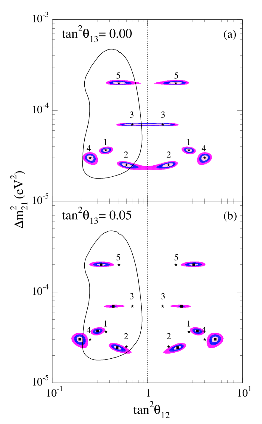
FIG. 1.: (a) Regions of the $(\Delta m^{2}_{21}\times\tan^{2}\theta_{12})$-parameter space allowed by three KamLAND-years of simulated data at the 1$\sigma$, 2$\sigma$ and 3$\sigma$ CL, for different input values of $\overline{\Delta m}^{2}_{21}$ and $\tan^{2}\overline{\theta_{12}}$ ($\overline{\theta_{13}}=0$) and assuming $\theta_{13}=0$. The stars indicate the best fit points (corresponding also to the simulated signals). (b) Regions of the $(\Delta m^{2}_{21}\times\tan^{2}\theta_{12})$-parameter space allowed by three KamLAND-years of simulated data at the 1$\sigma$, 2$\sigma$ and 3$\sigma$ CL for $\theta_{13}=12.6^{\circ}(\sin^{2}\theta_{13}=0.048)$. The stars indicate the points used to simulate the signal (with fixed $\overline{\theta_{13}}=0$) while the squares indicate the reconstructed best fit point (with fixed $\theta_{13}=12.6^{\circ}$).

The observed shift can be easily understood as follows. From Eq. (3), the total number of events is equal for different $\theta_{13}$ with the condition

$$1-\alpha\times\sin^{2}2\theta_{12}=\cos^{4}\theta_{13}(1-\alpha\times\sin^{2}2\theta^{\prime}_{12})\,,$$ (6)

where $\alpha$ is a number coming from all the detailed integration of the oscillating phase factor which depends mainly on $\Delta m^{2}_{12}$ and which, for completeness, we also list in Table I. For example for the simulated point (1), $\tan^{2}\overline{\theta_{12}}=0.37$, $\overline{\Delta m}_{12}^{2}=3.7\times 10^{-5}$ eV² and $\overline{\theta_{13}}=0$, the 3$\sigma$ reconstructed range, $0.31\leq\tan^{2}\theta_{12}\leq 0.43$, for $\theta_{13}=0$ is shifted using the above relation with $\alpha=0.65$ to $0.25\leq\tan^{2}\theta_{12}\leq 0.35$ for $\tan^{2}\theta_{13}=0.05$ which precisely coincides with the values listed in the 5th column of table I. Strictly speaking this scaling is slightly violated due to the change of the spectral shape with the change from $\theta_{12}$ to $\theta^{\prime}_{12}$ which also worsens the $\chi^{2}_{min}$ for the reconstructed point.

Let us finally consider which are the allowed regions in the parameter space $(\tan^{2}\theta_{12},\Delta m^{2}_{21})$ taking into account that we just know that $\theta_{13}$ is below some limit. In order to do so one must integrate over $\theta_{13}$ in the allowed range, or what is equivalent, for each pair $(\tan^{2}\theta_{12},\Delta m^{2}_{21})$ we must minimize $\chi^{2}(\theta_{12},\Delta m^{2}_{21},\tan^{2}\theta_{13})$ with respect to $\theta_{13}$ (restricted to be below the present bound). Notice that, below the bound, we used a flat probability distribution for $\theta_{13}$ to keep the analysis just KamLAND-dependent. In the future, the combined analysis of solar, atmospheric and CHOOZ results with KamLAMD data will allow us to include the probability distribution for $\theta_{13}$. In Fig. 2 we shown the allowed regions for such $\theta_{13}$-free analysis, where free means allowed to vary below its 3$\sigma$ limit, $\theta_{13}\leq 13.8^{\circ}$ ($\sin^{2}\theta_{13}\leq 0.057)$). As seen by comparing Fig. 2 with Fig. 1 the reconstructed regions are enlarged and roughly correspond to the overlap of the allowed regions for the different fixed values of $\theta_{13}$. Given our signal generating procedure the best fit reconstructed point corresponds to the simulated point in $(\tan^{2}\theta_{12}$, $\Delta m^{2}_{21})$ and $\theta_{13}=0$. The reconstructed ranges can be read from the last column in Tables I and Tables II. Also comparing the results in both tables one sees that the presence of this effect is not quantitatively affected by not including in the fit the data from the lowest energy bins. The main effect being a decrease in the statistics which translates into slightly larger ranges.

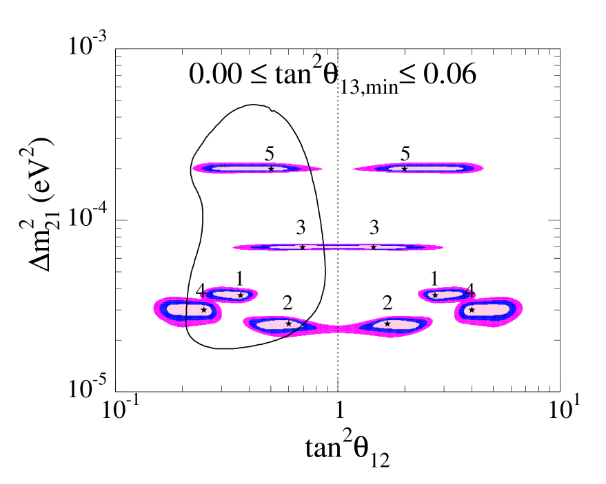
FIG. 2.: 1$\sigma$, 2$\sigma$ and 3$\sigma$ CL allowed regions of the $(\Delta m^{2}_{21}\times\tan^{2}\theta_{12})$-parameter space when $\theta_{13}$ is left free to vary in the allowed range ($\theta_{13}<13.8^{\circ}(\sin^{2}\theta_{13}=0.057)$). The regions are obtained for three KamLAND-years of simulated data and for the same five simulated signals as Fig.1(a). The stars indicate the best fit points (corresponding also to the simulated points).

Signal $\equiv$ ($\tan^{2}\overline{\theta_{12}},\overline{\Delta m}^{2}_{21},\overline{\theta_{13}}$)	$N_{ev}$	$\alpha$	$\theta_{13}=0$	$\theta_{13}=12.6^{\circ}(0.048)$	$\theta_{13}<13.8^{\circ}(0.057)$
1 $\equiv$ (0.37,3.7$\times 10^{-5}$,0)	1022	0.65	[0.31,0.43]	[0.25,0.35]	[0.24,0.43]
2 $\equiv$ (0.60,2.5$\times 10^{-5}$,0)	802	0.65	[0.48,1.00]	[0.39,0.68]	[0.38,1.00]
3 $\equiv$ (0.70,7.0$\times 10^{-5}$,0)	1335	0.56	[0.47,1.00]	[0.35,0.57]	[0.34,1.00]
4 $\equiv$ (0.25,3.0$\times 10^{-5}$,0)	1237	0.65	[0.21,0.30]	[0.16,0.24]	[0.15,0.30]
5 $\equiv$ (0.50,2.0$\times 10^{-4}$,0)	1321	0.44	[0.37,0.85]	[0.25,0.44]	[0.22,0.85]

TABLE I.: Reconstructed ranges for $\tan^{2}\theta_{12}$ at 3 $\sigma$ (in the first octant) for different $\theta_{13}$ ($\sin^{2}\theta_{13}$ in parenthesis) cases for the simulated points listed in the first column. See text for details.

Signal $\equiv$ ($\tan^{2}\overline{\theta_{12}},\overline{\Delta m}^{2}_{21},\overline{\theta_{13}}$)	$N_{ev}$	$\alpha$	$\theta_{13}=0$	$\theta_{13}=12.6^{\circ}(0.048)$	$\theta_{13}<13.8^{\circ}(0.057)$
1 $\equiv$ (0.37,3.7$\times 10^{-5}$,0)	756	0.65	[0.31,0.44]	[0.25,0.36]	[0.24,0.44]
2 $\equiv$ (0.60,2.5$\times 10^{-5}$,0)	695	0.72	[0.41,1.00]	[0.35,1.00]	[0.34,1.00]
3 $\equiv$ (0.70,7.0$\times 10^{-5}$,0)	1167	0.52	[0.44,1.00]	[0.32,0.59]	[0.31,1.00]
4 $\equiv$ (0.25,3.0$\times 10^{-5}$,0)	1004	0.65	[0.20,0.42]	[0.15,0.68]	[0.14,1.00]
5 $\equiv$ (0.50,2.0$\times 10^{-4}$,0)	1090	0.44	[0.36,1.00]	[0.24,0.46]	[0.22,1.00]

TABLE II.: Same as table 1 after removing the lower energy bins from the fit (therefore including only events with $2.72<E_{vis}<7.22$ MeV).

We have studied the role of $\theta_{13}$ in the hypothetical case of perfect knowledge of the overall flux normalization and fuel composition. Comparing our results with the expected degradation on the parameter determination associated with the uncertainty on those two assumptions  [16], we note that the reconstructed ranges obtained in the $\theta_{13}$-free case are very close to those obtained in the analysis with perfect knowledge of $\theta_{13}$ but where the overall flux normalization is unknown by about $\sim$ 10%. As mentioned above, the role of $\theta_{13}$ is essentially the change of the normalization. This is a larger normalization error that the 3% expected one in the theoretical calculation of the flux from the reactors (induced from the $\beta$-spectroscopy experiment at the Goesgen reactor [26]). We also find that the uncertainty associated with $\theta_{13}$ has a larger impact on the determination of the mixing angle $\theta_{12}$ than the expected error associated with the fuel composition although, unlike this last one, it does not affect the determination of $\Delta m^{2}_{12}$.

Let us point out, that obviously, in order for this effect to become relevant it has to be larger than the expected statistical uncertainty on the overall flux normalization. If we repeat this exercise assuming only one KamLAND-years of simulated data, we find very little difference between the results corresponding to fixed $\theta_{13}=0$ and the free-$\theta_{13}$ analysis, as expected since the expected number of events would be of the order $\sim 400$ and the associated statistical uncertainty for the overall normalization would be comparable with the maximum effect associated to $\theta_{13}$.

Summarizing, the KamLAND reactor neutrino experiment, which is to start taking data very soon, is sensitive to the LMA region and should be able of measuring the solar oscillation parameters $(\tan^{2}\theta_{12},\Delta m^{2}_{21})$ with unprecedented precision. In this letter, we have addressed the question of the degradation on the determination of the oscillation parameters associated with our ignorance of the exact value of $\theta_{13}$. We have shown that the determination of $\Delta m_{12}^{2}$ is practically unaffected because the effect of $\theta_{13}$ on the shape of the spectrum is very small. The dominant effect is a shift in the overall flux normalization which implies that the reconstructed $\theta_{12}$ range scales with $\theta_{13}$ in a simple way. As a consequence the allowed region of solar parameters obtained from KamLAND signal will be broader in $\theta_{12}$. Comparing this effect with the ones from the expected uncertainties associated with the theoretical error on the overall flux normalization and the fuel composition, we find that, after enough statistics is accumulated, the uncertainty associated with $\theta_{13}$ may become the dominant source of degradation in the determination of the mixing angle $\theta_{12}$ at KamLAND.