ON BUILDING BETTER CONE JET ALGORITHMS

Abstract

We discuss recent progress in understanding the issues essential to the development of better cone jet algorithms.

An important facet of preparationsworkshops for Run II at the Tevatron, and for future data taking at the LHC, has been the study of ways in which to improve jet algorithms.  These algorithms are employed to map final states, both in QCD perturbation theory and in the data, onto jets.  The motivating idea is that these jets are the surrogates for the underlying energetic partons.  In principle, we can connect the observed final states, in all of their complexity, with the perturbative final states, which are easier to interpret and to analyze theoretically.  Of necessity these jet algorithms should be robust under the impact of both higher order perturbative and non-perturbative physics and the effects introduced by the detectors themselves.  The quantitative goal is a precision of order 1% in the mapping between theory and experiment.  In this note we will provide a brief summary of recent progress towards this goal.  A more complete discussion of our results will be provided elsewherelongpaper .  Here we will focus on cone jet algorithms, which have formed the basis of jet studies at hadron colliders.

As a starting point we take the Snowmass AlgorithmSnowmass , which was defined by a collaboration of theorists and experimentalists and formed the basis of the jet algorithms used by the CDF and DØ collaborations during Run I at the Tevatron.  Clearly jets are to be composed of either hadrons or partons that are, in some sense, nearby each other.  The cone jet defines nearness in an intuitive geometric fashion: jets are composed of hadrons or partons whose 3-momenta lie within a cone defined by a circle in $\left(\eta,\phi\right)$.  These are essentially the usual angular variables, where $\eta=\ln\left(\cot\,\theta/2\right)$ is the pseudorapidity and $\phi$ is the azimuthal angle. This idea of being nearby in angle can be contrasted with an algorithm based on being nearby in transverse momentum as illustrated by the so-called $k_{T}$ Algorithmktcluster that has been widely used at $e^{+}e^{-}$ and $ep$ colliders.  We also expect the jets to be aligned with the most energetic particles in the final state.  This expectation is realized in the Snowmass Algorithm by defining an acceptable jet in terms of a “stable” cone such that the geometric center of the cone is identical to the $E_{T\text{ }}$ weighted centroid.  Thus, if we think of a sum over final state partons or hadrons defined by an index $k$ and in the direction $\left(\eta_{k},\phi_{k}\right)$, a jet ($J$) of cone radius $R$ is defined by the following set of equations

$$k \in J:\left(\phi_{k}-\phi_{J}\right)^{2}+\left(\eta_{k}-\eta_{J}\right)^{2}\leq R^{2},$$

$$\phi_{J} =\sum_{k\in J}\frac{E_{T,k}\phi_{k}}{E_{T,J}},\quad\eta_{J}=\sum_{k\in J}\frac{E_{T,k}\eta_{k}}{E_{T,J}},$$ (1)

$$E_{T,J} =\sum_{k\in J}E_{T,k}.$$

In these expressions $E_{T}$ is the transverse energy ($\left|\overrightarrow{p}_{T}\right|$ for a massless 4-vector).  It is important to recognize that jet algorithms involve two distinct steps.  The first step is to identify the “members” of the jet, i.e., the calorimeter towers or the partons that make-up the stable cone that becomes the jet.  The second step involves constructing the kinematic properties that will characterize the jet, i.e., determine into which bin the jet will be placed.  In the original Snowmass Algorithm the $E_{T}$ weighted variables defined in Eq. 1 are used both to identify and bin the jet.

In a theoretical calculation one integrates over the phase space corresponding to parton configurations that satisfy the stability conditions.  In the experimental case one searches for sets of final state particles (and calorimeter towers) in each event that satisfy the constraint.  In practiceworkshops the experimental implementation of the cone algorithm has involved the use of various short cuts to minimize the search time.  In particular, Run I algorithms made use of seeds.  Thus one looks for stable cones only in the neighborhood of calorimeter cells, the seed cells, where the deposited energy exceeds a predefined limit.  Starting with such a seed cell, one makes a list of the particles (towers) within a distance $R$ of the seed and calculates the centroid for the particles in the list (calculated as in Eq. 1).  If the calculated centroid is consistent with the initial cone center, a stable cone has been identified.  If not, the calculated centroid is used as the center of a new cone with a new list of particles inside and the calculation of the centroid is repeated.  This process is iterated, with the cone center migrating with each repetition, until a stable cone is identified or until the cone centroid has migrated out of the fiducial volume of the detector.  When all of the stable cones in an event have been identified, there will typically be some overlap between cones.  This situation must be addressed by a splitting/merging routine in the jet algorithm.  This feature was not foreseen in the original Snowmass Algorithm.  Normally this involves the definition of a parameter $f_{merge}$, typically with values in the range $0.5\ \leq f_{merge}\leq 0.75,$ such that, if the overlap transverse energy fraction (the transverse energy in the overlap region divided by the smaller of the total energies in the two overlapping cones) is greater than $f_{merge}$, the two cones are merged to make a single jet. If this constraint is not met, the calorimeter towers/hadrons in the overlap region are individually assigned to the cone whose center is closer.  This situation yields 2 final jets.

The essential challenge in the use of jet algorithms is to understand the differences between the experimentally applied algorithms and the theoretically applied ones and hence understand the uncertainties.  This is the primary concern of this paper.  It has been known for some time that the use of seeds in the experimental algorithms means that certain configurations kept by the theoretical algorithm are likely to be missed by the experimental oneSDERsep .  At higher orders in perturbation theory the seed definition also introduces an undesirable (logarithmic) dependence on the seed $E_{T}$ cut (the minimum $E_{T}$ required to be treated as a seed cell)Seymour .  Various alternative algorithms are described in the Run II Workshop proceedingsworkshops for addressing this issue, including the Midpoint Algorithm and the Seedless Algorithm.  In the last year it has also been recognized that other final state configurations are likely to be missed in the data, compared to the theoretical result.  In this paper we will explain these new developments and present possible solutions.  To see that there is a problem, we apply representative jet algorithms to data sets that were generated with the HERWIG Monte CarloHerwig and then run through a CDF detector simulation.  As a reference we include in our analysis the JetClu AlgorithmJetClu , which is the algorithm used by CDF in Run I.  It employs both seeds and a property called “ratcheting”.  This latter term labels the fact that the Run I CDF algorithm (unlike the corresponding DØ algorithm) was defined so that calorimeter towers initially found in a cone around a seed continue to be associated with that cone, even as the center of the cone migrates due to the iteration of the cone algorithm.  Thus the final “footprint” of the cone is not necessarily a circle in $\left(\eta,\phi\right)$ (even before the effects of splitting/merging).  Since the cone is “tied” to the initial seed towers, this feature makes it unlikely that cones will migrate very far before becoming stable. We describe results from JetClu both with and without this ratcheting feature.  The second cone algorithm studied is the Midpoint Algorithm that, like the JetClu Algorithm, starts with seeds to find stable cones (but without ratcheting). The Midpoint Algorithm then adds a cone at the midpoint in $\left(\eta,\phi\right)$ between all identified pairs of stable cones separated by less than $2R$ and iterates this cone to test for stability.  This step is meant to ensure that no stable “mid-cones” are missed, compared to the theoretical result, due to the use of seeds.  Following the recommendation of the Run II Workshop, we actually use 4-vector kinematics for the Midpoint Algorithm and place the cone at the midpoint in $\left(y,\phi\right)$, where $y$ is the true rapidity.  The third cone algorithm is the Seedless Algorithm that places an initial trial cone at every point on a regular lattice in $\left(y,\phi\right)$, which is approximately as fine-grained as the detector.  It is not so much that this algorithm lacks seeds, but rather that the algorithm puts seed cones “everywhere”.  The Seedless Algorithm can be streamlined by imposing the constraint that a given trial cone is removed from the analysis if the center of the cone migrates outside of its original lattice cell during the iteration process.  The streamlined version still samples every lattice cell for stable cone locations, but is less computationally intensive.  Our experience with the streamlined version of this algorithm suggests that there can be problems finding stable cones with centers located very close to cell boundaries.  This technical difficulty is easily addressed by enlarging the distance that a trial cone must migrate before being discarded.  For example, if this distance is 60% of the lattice cell width instead of the default value of 50%, the problem essentially disappears with only a tiny impact on the required time for analysis.  In the JetClu Algorithm the value $f_{merge}=0.75$ was used (as in the Run I analyses), while for the other two cone algorithms the value $f_{merge}=0.5$ was used as suggested in the Workshop Proceedingsworkshops .   Finally, for completeness, we include in our analysis a sample $k_{T}$ Algorithm.

Starting with a sample of 250,000 events, which were generated with HERWIG 6.1 and run through a CDF detector simulation and which were required to have at least 1 initial parton with $E_{T}>200$ GeV, we applied the various algorithms to find jets with $R=0.7$ in the central region ($\left|\eta\right|<1$).  We then identified the corresponding jets from each algorithm by finding jet centers differing by $\Delta R<0.1$.  The plots in Fig. 1 indicate the average difference in $E_{T}$ for these jets as a function of the jet $E_{T}$.  (We believe that some features of the indicated structure, in particular the “knees” near $E_{T}=150$ GeV, are artifacts of the event selection process.)

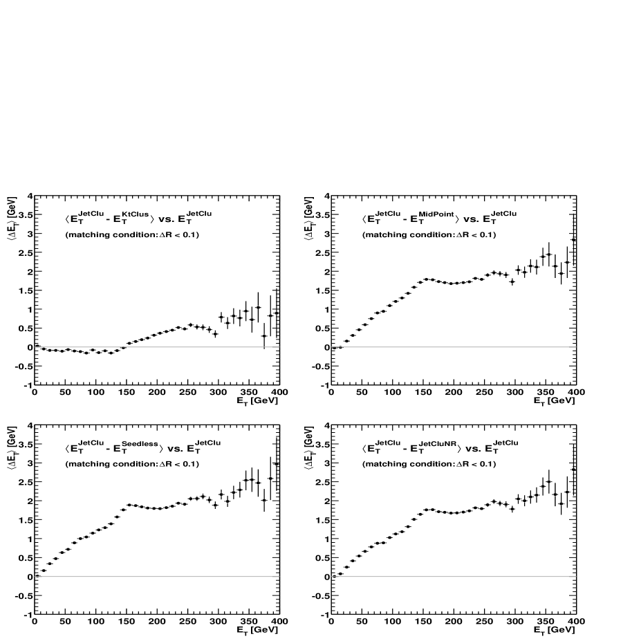
Figure 1: Difference of $E_{T}$ for matched jets found with various jet algorithms and compared to the JetClu CDF Run I algorithm.  The events studied were generated with HERWIG 6.1 and run through the CDF detector simulation.

From these results we can draw several conclusions.  First, the $k_{T}$ Algorithm identifies jets with $E_{T}$ values similar to those found by JetClu, finding slightly more energetic jets at small $E_{T}$ and somewhat less energetic jets at large $E_{T}$.  We will not discuss this algorithm further here except to note that DØ has applied it in a study of Run I dataD0 and in that analysis the $k_{T}$ Algorithm jets seems to exhibit slightly larger $E_{T}$ than expected from NLO perturbation theory. The cone algorithms, including the JetClu Algorithm without ratcheting, which is labeled JetCluNR, identify jets with approximately 0.5% to 1 % smaller $E_{T}$ values than those identified by the JetClu Algorithm (with ratcheting), with a corresponding approximately 5% smaller jet cross section at a given $E_{T}$ value.  We believe that this systematic shortfall can be understood as resulting from the smearing effects of perturbative showering and non-perturbative hadronization.

To provide insight into the issues raised by Fig. 1 we now discuss a simple, but informative analytic picture.  It will serve to illustrate the impact of showering and hadronization on the operation of jet algorithms.  We consider the scalar function $F\left(\overrightarrow{r}\right)$ defined as a function of the 2-dimensional variable $\overrightarrow{r}=\left(\eta,\phi\right)$ by the integral over the transverse energy distribution of either the partons or the hadrons/calorimeter towers in the final state with the indicated weight function,

$$F\left(\overrightarrow{r}\right) =\frac{1}{2}\int d^{2}\rho\times\left(R^{2}-\left(\overrightarrow{\rho}-\overrightarrow{r}\right)^{2}\right)\times\,\Theta\left(R^{2}-\left(\overrightarrow{\rho}-\overrightarrow{r}\right)^{2}\right)\times E_{T}\left(\overrightarrow{\rho}\right)$$ (2)

$$=\frac{1}{2}\sum_{i}E_{T,i}\times\left(R^{2}-\left(\overrightarrow{\rho_{i}}-\overrightarrow{r}\right)^{2}\right)\times\,\Theta\left(R^{2}-\left(\overrightarrow{\rho_{i}}-\overrightarrow{r}\right)^{2}\right).$$

The second expression arises from replacing the continuous energy distribution with a discrete set, $i=1$ to $N,$ of delta functions, representing the contributions of either a configuration of partons or a set of calorimeter towers (and hadrons).  Each parton direction or the location of the center of each calorimeter tower is defined in $\eta$, $\phi$ by $\rho_{i}=\left(\eta_{i},\phi_{i}\right)$, while the parton/calorimeter cell has a transverse energy (or $E_{T}$) content given by $E_{T,i}$.  This function is clearly related to the energy in a cone of size $R$ containing the towers whose centers lie within a circle of radius $R$ around the point $\overrightarrow{r}$.  More importantly it carries information about the locations of “stable” cones.  The points of equality between the $E_{T}$ weighted centroid and the geometric center of the cone correspond precisely to the maxima of $F$.  The gradient of this function has the form (note that the delta function arising from the derivative of the theta function cannot contribute as it is multiplied by a factor equal to its argument)

$$\overrightarrow{\nabla}F\left(\overrightarrow{r}\right)=\sum_{i}E_{T,i}\times\left(\overrightarrow{\rho_{i}}-\overrightarrow{r}\right)\times\Theta\left(R^{2}-\left(\overrightarrow{\rho_{i}}-\overrightarrow{r}\right)^{2}\right).$$ (3)

This expression vanishes at points where the weighted centroid coincides with the geometric center, i.e., at points of stability (and at minima of $F$, points of extreme instability).  The corresponding expression for the energy in the cone centered at $\overrightarrow{r}$ is

$$E_{C}\left(\overrightarrow{r}\right)=\sum_{i}E_{T,i}\times\Theta\left(R^{2}-\left(\overrightarrow{\rho_{i}}-\overrightarrow{r}\right)^{2}\right).$$ (4)

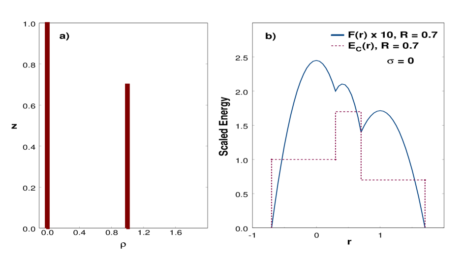
Figure 2: 2-Parton distribution: a) transverse energy distribution; b) distributions F(r) and E_C(r) in the perturbative limit of no smearing.

To more easily develop our understanding of these equations consider a simplified scenario (containing all of the interesting effects) involving 2 partons separated in just one angular dimension $\overrightarrow{\rho}\rightarrow\rho$ ($\overrightarrow{r}\rightarrow r$) with $\rho_{2}-\rho_{1}=d$.  It is sufficient to specify the energies of the 2 partons simply by their ratio, $z=E_{2}/E_{1}\leq 1$.  Now we can study what sorts of 2 parton configurations yield stable cones in this 2-D phase space specified by $0\leq z\leq 1$, $0\leq d\leq 2R$ (beyond $2R$ the 2 partons are surely in different cones).  As a specific example consider the case $\rho_{1}=0$, $\rho_{2}=d=1.0$ and $z=0.7$ with $R=0.7$ (the typical experimental value).  The underlying energy distribution is illustrated in Fig. 2a, representing a delta function at $\rho=0$ (with scaled weight 1) and another at $\rho=1.0$ (with scaled weight 0.7).  This simple distribution leads to the functions $F(r)$ and $E_{C}(r)$ indicated in Fig. 2b.  In going from the true energy distribution to the distribution $E_{C}(r)$ the energy is effectively smeared over a range given by $R$.  In $F(r)$ the distribution is further shaped by the quadratic factor $R^{2}-\left(\rho_{i}-r\right)^{2}$.  We see that $F(r)$ exhibits 3 local maxima corresponding to the expected stable cones around the two original delta functions ($r_{1}=0,r_{2}=1$), plus a third stable cone in the middle ($r_{3}=zd/\left(1+z\right)=0.41$ in the current case).  This middle cone includes the contributions from both partons as indicated by the magnitude of the middle peak in the function $E_{C}(r)$.  Note further that the middle cone is found at a location where there is initially no energy in Fig. 2a, and thus no seeds.  One naively expects that such a configuration is not identified as a stable cone by the experimental implementations of the cone algorithm that use seeds simply because they do not look for it.  Note also that, since both partons are entirely within the center cone, the overlap fractions are unity and the usual merging/splitting routine will lead to a single jet containing all of the initial energy ($1+z$).  This is precisely how this configuration was treated in the NLO perturbative analysis of the Snowmass AlgorithmEKS (i.e., only the leading jet, the middle cone, was kept).

Similar reasoning leads to Fig. 3a, which indicates the various 2 parton configurations found by the perturbative cone algorithm.  For $d<R$ one finds a single stable cone and a single jet containing both partons.  For $R<d<(1+z)R$ one finds 3 stable cones that merge to 1 jet, again with all of the energy.  For $d>(1+z)R$  we find 2 stable cones and 2 jets, each containing one parton, of scaled energies $1$ and $z$.  Thus, except in the far right region of the graph, the 2 partons are always merged to form a single jet.

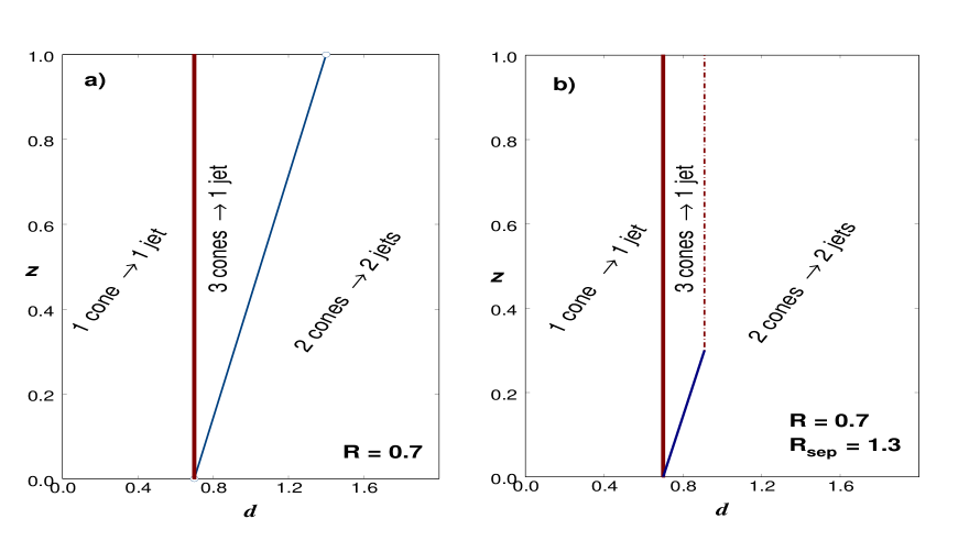
Figure 3: Perturbation Theory Structure: a) $R_{sep}=2$; b) $R_{sep}=1.3$.

We expect that the impact of seeds in experimental algorithms can be (crudely) simulated in the NLO calculationsSDERsep by including a parameter $R_{sep}$ such that stable cones containing 2 partons are not allowed for partons separated by $d>R_{sep}\times R$.  As a result cones are no longer merged in this kinematic region.  In the present language this situation is illustrated in Fig. 3b corresponding to $R_{sep}=1.3$, $R\times R_{sep}=0.91$.  This specific value for $R_{sep}$ was chosenSDERsep to yield reasonable agreement with the Run I data.  The conversion of much the 3 cones $\rightarrow$ 1 jet region to 2 cones $\rightarrow$ 2 jets has the impact of lowering the average $E_{T}$ of the leading jet and hence the jet cross section at a fixed $E_{T,J}$.  Parton configurations that naively produced jets with energy characterized by $1+z$ now correspond to jets of maximum energy 1.  This is just the expected impact of a jet algorithm with seeds.  Note that with this value of $R_{sep}$ the specific parton configuration in Fig. 2a will yield 2 jets (and not 1 merged jet) in the theoretical calculation.  As mentioned earlier this issue is to be addressed by the Midpoint and Seedless Algorithms in Run II.  However, as indicated in Fig. 1, neither of these two algorithms reproduces the results of JetClu.  Further, they both identify jets that are similar to JetClu without ratcheting.  Thus we expect that there is more to this story.

As suggested earlier, a major difference between the perturbative level, with a small number of partons, and the experimental level of multiple hadrons is the smearing that results from perturbative showering and nonperturbative hadronization.  For the present discussion the primary impact is that the starting energy distribution will be smeared out in the variable $r$.  We can simulate this effect in our simple model using gaussian smearing, i.e., we replace the delta functions in Eq. 2 with gaussians of width $\sigma$.  (Since this corresponds to smearing in an angular variable, we would expect $\sigma$ to be a decreasing function of $E_{T}$, i.e., more energetic jets are narrower.  We also note that this naive picture does not include the expected color coherence in the products of the showering/hadronization process.)  The first impact of this smearing is that some of the energy initially associated with the partons now lies outside of the cones centered on the partons.  This effect, typically referred to as “splashout” in the literature, is (exponentially) small in this model for $\sigma<R$.  Here we will focus on less well known but phenomenologically more relevant impacts of splashout. The distributions corresponding to Fig. 2b, but now with $\sigma=0.10$ (instead of $\sigma=0$), are exhibited in Fig. 4a.

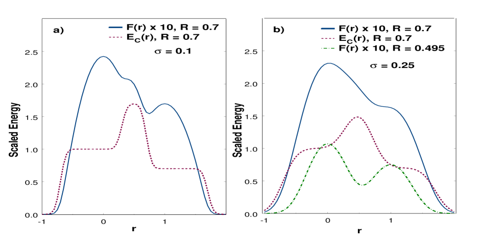
Figure 4: The distributions F(r) and E_C(r) for smearing width a) 0.1; b) 0.25.

With the initial energy distribution smeared by $\sigma$, the distribution $F(r)$ is now even more smeared and, in fact, we see that the middle stable cone (the maximum in the middle of Fig. 2b) has been washed out by the increased smearing.  Thus the cone algorithm applied to data (where such smearing is present) may not find the middle cone that is present in perturbation theory, not only due to the use of seeds but also due to this new variety of splashout correction, which renders this cone unstable.  Since, as a result of this splashout correction, the middle cone is not stable, this problem is not addressed by either the Midpoint Algorithm or the Seedless Algorithm.  Both algorithms may look in the correct place, but they look for stable cones.  This point is presumably part of the explanation for why both of these algorithms disagree with the JetClu results in Fig. 1.

Our studies also suggest a further impact of the smearing of showering/hadronization that was previously unappreciated.  This new effect is illustrated in Fig. 4b, which shows $F(r)$, still for $z=0.7$ and $d=1.0,$ but now for $\sigma=0.25$.  With the increased smearing the second stable cone, corresponding to the second parton, has now also been washed out, i.e., the right hand local maximum has also disappeared.  This situation is exhibited in the case of “data” by the lego plot in Fig. 5 indicating the jets found by the Midpoint Algorithm in a specific Monte Carlo event.  The Midpoint Algorithm does not identify the energetic towers (shaded in black) to the right of the energetic central jet as either part of that jet or as a separate jet, i.e., these obviously relevant towers are not found to be in a stable cone.  The iteration of any cone containing these towers invariably migrates to the nearby higher $E_{T}$ towers.

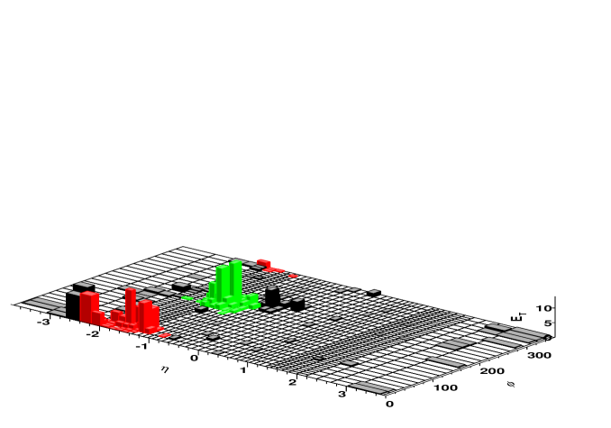
Figure 5: Result of applying the Midpoint Algorithm to a specific Monte Carlo event in the CDF detector.

In summary, we have found that the impact of smearing and splashout is expected to be much more important than simply the leaking of energy out of the cone.  Certain stable cone configurations, present at the perturbative level, can disappear from the analysis of real data due to the effects of showering and hadronization.  This situation leads to corrections to the final jet yields that are relevant to our goal of 1% precision in the mapping between perturbation theory and experiment.  Compared to the perturbative analysis of the 2-parton configuration, both the middle stable cone and the stable cone centered on the lower energy parton can be washed out by smearing.  Further, this situation is not addressed by either the Midpoint Algorithm or the Seedless Algorithm.  One possibility for addressing the missing middle cone would be to eliminate the stability requirement for the added midpoint cone in the Midpoint Algorithm.  However, if there is enough smearing to eliminate also the second (lower energy) cone, even this scenario will not help, as we do not find two cones to put a third cone between.  There is, in fact, a rather simple “fix” that can be applied to the Midpoint Algorithm to address this latter form of the splashout correction.  We can simply use 2 values for the cone radius $R$, one during the search for the stable cones and the second during the calculation of the jet properties.  As a simple example, the 3rd curve in Fig. 4b corresponds to using $R/\sqrt{2}=0.495$ during the stable cone discovery phase and $R=0.7$ in the jet construction phase.  Thus the $R/\sqrt{2}$ value is used only during iteration; the cone size is set to $R$ right after the stable cones have been identified and the larger cone size is employed during the splitting/merging phase.  By comparing Figs. 4b and 2b we see that the two outer stable cones in the perturbative case are in essentially the same locations as in the smeared case using the smaller cone during discovery.  The improved agreement between the JetClu results and those of the Midpoint Algorithm with the last “fix” (using the smaller $R$ value during discovering but still requiring cones to be stable) are indicated in Fig. 6.

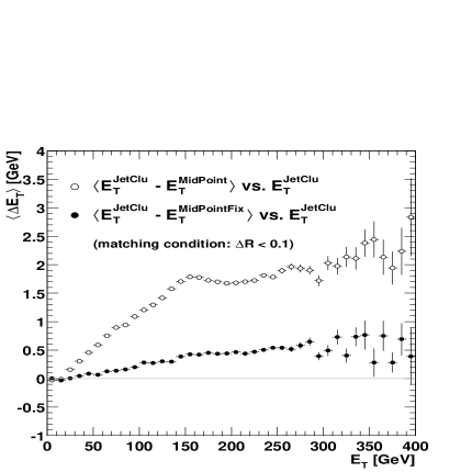
Figure 6: The difference in the $E_{T}$ of identified central jets for the JetClu and Midpoint Algorithms, both with and without the “fix” discussed in the text.  The events studied were generated with HERWIG 6.1 and run through the CDF detector simulation.

Clearly most, but not all, of the differences between the jets found by the JetClu and Midpoint Algorithms are removed in the fixed version of the latter.  The small $R$ “fix” suggested for the Midpoint Algorithm can also be employed for the Seedless Algorithm but, like the Midpoint Algorithm, it will still miss the middle (now unstable) cone.

Before closing this brief summary of our results, we should say a few more words about the Run I CDF algorithm that we used as a reference.  In particular, while ratcheting is difficult to simulate in perturbation theory, we can attempt to clarify how it fits into the current discussion.  As noted above, the JetClu Algorithm is defined so that calorimeter towers initially found around a seed stay with that cone, even as the center of the cone migrates due to the iteration of the cone algorithm.  For the simple scenario illustrated in Fig. 2a we assume that the locations of the partons are identified as seeds, even when smearing is present.  To include both ratcheting and the way it influences the progress of the stable cone search, we must define 2 scalar functions of the form of Eq. 2, one to simulate the search for a stable cone starting at $\rho=0$ and the second for the search starting at $\rho=1.0$.  The former function is defined to include the energy within the range $-R\leq\rho\leq+R$ independent of the value of $r$, while the second function is defined to always include the energy in the range $1.0-R\leq\rho\leq 1.0+R.$  Analyzing the two functions defined in this way suggests, as expected, that the search that begins at the higher energy seed will always find a stable cone at the location of that seed, independent of the amount of smearing.  (If the smearing is small, there is also a stable cone at the middle location but the search will terminate after finding the initial, nearby stable cone.)  The more surprising result arises from analyzing the second function, which characterizes the search for a stable cone seeded by the lower energy parton. In the presence of a small amount of smearing this function indicates stable cones at both the location of the lower energy parton and at the middle location.  Thus the corresponding search finds a stable cone at the position of the seed and again will terminate before finding the second stable cone.  When the smearing is large enough to wash out the stable cone at the second seed, the effect of ratcheting is to ensure that the search still finds a stable cone at the middle location suggested by the perturbative result, $r_{3}=z\rho/\left(1+z\right)$ (with a precision given by $\sigma\times e^{-\left(R/\sigma\right)^{2}}$).  This result suggests that the JetClu Algorithm with ratcheting always identifies either stable cones at the location of the seeds or finds a stable cone in the middle that can lead to merging (in the case of large smearing).  It is presumably just these last configurations that lead to the remaining difference between the JetClu Algorithm results and those of the “fixed” Midpoint Algorithm illustrated in Fig. 6.  We find that the jets found by the JetClu Algorithm have the largest $E_{T}$ values of any of the cone jet algorithms, although the JetClu Algorithm still does not address the full range of splashout corrections.

In conclusion, we have found that the corrections due to the splashout effects of showering and hadronization result in unexpected differences between cone jet algorithms applied to perturbative final states and applied to (simulated) data. With a better understanding of these effects, we have defined steps that serve to improve the experimental cone algorithms and minimize these corrections.  Further studies are required to meet the goal of 1% agreement between theoretical and experimental applications of cone algorithms.

- (1) G. C. Blazey, et al., Run II Jet Physics: Proceedings of the Run II QCD and Weak Boson Physics Workshop, hep-ex/0005012; P. Aurenche, et al., The QCD and Standard Model Working Group: Summary Report from Les Houches, hep-ph/0005114.
- (2) S.D. Ellis, J. Huston and M. Tönnesmann, in preparation.
- (3) J. E. Huth, et al., in Proceedings of Research Directions for the Decade: Snowmass 1990, July 1990, edited by E. L. Berger (World Scientific, Singapore, 1992) p. 134.
- (4) S.D. Ellis and D. Soper, Phys. Rev. D48, 3160 (1993); S. Catani, Yu.L. Dokshitzer and B.R. Webber, Phys. Lett. B285, 291 (1992); S. Catani, Yu.L. Dokshitzer, M.H. Seymour and B.R. Webber, Nucl. Phys. B406, 187 (1993).
- (5) S.D. Ellis, Z. Kunszt and D. Soper, Phys. Rev Lett. 69, 3615 (1992); S.D. Ellis in Proceedings of the 28th Rencontres de Moriond: QCD and High Energy Hadronic Interactions, March 1993, p. 235; B. Abbott, et al., Fermilab Pub-97-242-E (1997).
- (6) M.H. Seymour, Nucl. Phys. B513, 269 (1998).
- (7) G. Marchesini, B.R. Webber, G. Abbiendi, I.G. Knowles, M.H. Seymour, L. Stanco, Computer Phys. Commun. 67, 465 (1992) ; G. Corcella, I.G. Knowles, G. Marchesini, S. Moretti, K. Odagiri, P. Richardson, M.H. Seymour, B.R. Webber, JHEP 01, 010 (2001) [hep-ph/9912396].
- (8) F. Abe et al. (CDF Collaboration), Phys. Rev. D45, 1448 (1992).
- (9) DØ Collaboration, V.M. Abazov, et al., hep-ex/0106032.
- (10) S.D. Ellis, Z. Kunszt and D. Soper, Phys. Rev Lett. 69, 1496 (1992); Phys. Rev Lett. 64, 2121 (1990); Phys. Rev. D40, 2188 (1989); Phys. Rev. Lett. 62, 726 (1989).