On the Evolution of Abelian-Higgs String Networks

Abstract

We study the evolution of Abelian-Higgs string networks in large-scale numerical simulations in both a static and expanding background. We measure the properties of the network by tracing the motion of the string cores, for the first time estimating the rms velocity of the strings and the invariant string length, that is, the true network energy density. These results are compared with a velocity-dependent one scale model for cosmic string network evolution. This incorporates the contributions of loop production, massive radiation and friction to the energy loss processes that are required for scaling evolution. We use this analysis as a basis for discussing the relative importance of these mechanisms for the evolution of the network. We find that the loop distribution statistics in the simulations are consistent with the long-time scaling of the network being dominated by loop production. Making justifiable extrapolations to cosmological scales, these results appear to be consistent with the standard picture of local string network evolution in which loop production and gravitational radiation are the dominant decay mechanisms.

I Introduction

Vortex-string networks in three dimensions are important in a variety of contexts, whether in condensed matter physics or cosmology (for reviews see [1, 2, 3]). If we are to obtain a quantitative description of these networks, then we must develop an adequate understanding of their ‘scaling’ evolution as well as the decay mechanisms which maintain it. The Abelian-Higgs model, a relativistic version of the Ginsburg-Landau theory of superconductors, provides a convenient testbed for developing detailed models for this evolution. On the one hand, the relatively simple field theory can be studied directly in three-dimensional simulations. On the other, a straightforward reduction to a one-dimensional effective theory—the Nambu action—can also be studied numerically, though over a much wider dynamic range.

In a cosmological context, a rather simple ‘one-scale’ model of string evolution has emerged [4, 5] which appears to successfully describe the large-scale features of an evolving string network [6, 7], though with subtleties remaining on smaller scales. In this simple model, after an initial transient period, the average number of long strings in a horizon volume remains fixed as it expands, a rapid dilution made possible through re-connections resulting in loop production. The loops, in this standard picture, oscillate relativistically and decay through gravitational radiation. The subtlety here concerns the length scale at which small loop creation occurs and whether this is inherently scale-invariant [8, 9]. Even if this were not so, additional gravitational radiation back-reaction effects should act on the long string network, eliminating small wavelength modes and thus setting a minimum loop creation size which is scale-invariant[6, 8]. In any case, high resolution Nambu string simulations have found that large-scale network properties are relatively insensitive to this loop creation scale, below a minimum loop size [6, 7].

This standard picture for network evolution has been questioned on the basis of Abelian-Higgs field theory simulations [10], as well as the correspondence between the Nambu simulations and global field theory simulations [15, 16]. In the first case [10], the authors suggested that the primary energy loss mechanism by long strings is direct massive radiation, rather than loop creation (we denote this as the ‘scale-invariant massive radiation’ scenario). This is contrary to previous expectations that the presence of a large mass threshold will strongly suppress massive particle production for long wavelength oscillatory string modes, that is, those much larger than the string width [11, 12, 13, 14]. Evidence presented in support of this includes Smith-Vilenkin simulations in which scaling is observed only if strings are produced at the smallest available scales, the profusion of loops at resolution scale in other Nambu codes, field theory network simulations in which the loop density is observed to be low, and the study of large amplitude oscillations of a single string.

The primary purpose of this paper is to study an evolving string network and its decay mechanisms. This involves extensive large-scale numerical simulations of Abelian-Higgs string networks in flat and expanding backgrounds. Simulations in an expanding universe, in particular, are severely limited in dynamic range so we also explore a new “fat string” algorithm appropriate for gauged strings, which keeps the string width constant in comoving coordinates. For comparison with a theory that is known to be strongly radiating, we simulated global strings in an expanding background (studied previously by Yamaguchi and collaborators [15, 16]). Having characterised the initial scaling properties of an Abelian-Higgs network, we endeavour to model the dominant decay mechanisms using the velocity-dependent one-scale (VOS) model. In order to achieve this, we have developed a new suite of diagnostic tools to estimate both the (static) string length and the average rms velocity of the network. The latter is challenging and has not been attempted in previous work but it is important, first, if we are to estimate the true (invariant) string length and, secondly, because it can be used to distinguish between different network decay mechanisms. We find some reasonable best-fit parameters for the VOS model which are self-consistent across all backgrounds (flat or expanding) and, on this basis, we are able to eliminate a number of scenarios. Finally, we conclude with a qualitative study of loop production in these networks. We emphasise the care which must be exercised in trying to extrapolate these field theory simulation results by many orders of magnitude to cosmological scales.

II String network evolution

A Simulation methods

The work in this paper involves simulations of systems, in flat or FRW backgrounds, arising from the Abelian-Higgs Lagrangian:

$${\mathcal{L}}=D_{\mu}\phi^{*}D^{\mu}\phi-\frac{1}{4}F_{\mu\nu}F^{\mu\nu}-\frac{\lambda}{4}(|\phi|^{2}-\eta^{2})^{2},$$ (1)

which yields the corresponding equations of motion,

$$D_{\mu}D^{\mu}\phi = -\frac{\lambda\phi}{2}(|\phi|^{2}-\eta^{2}),$$ (2)

$$J^{\mu}\equiv\partial_{\nu}F^{\nu\mu} = 2e{\rm Im}(\phi^{*}D^{\mu}\phi).$$ (3)

Allowing for the rescaling of coordinates and the Higgs field, the only free parameter in the model is the ratio $\beta\equiv\lambda/2e^{2}$. The critial value $\beta=1$ is the well-known Bogomolyni limit in which the scalar and vector forces between like vortices cancel.

Following Moriarty et al. [28], it has become standard to simulate the dynamics of the abelian-Higgs model using an approach derived from lattice gauge theory. The Lagrangian density is transformed to a Hamiltonian one and discretised on a lattice of spacing $d$, in the gauge $A_{0}=0$. With this formalism the Higgs field variables are associated with the vertices of the simulation lattice, while the gauge fields are associated with the links. To evolve the initial configurations forward in time we use a leap-frog method, using centered derivatives for the time evolution. The configuration space and momentum space variables are interleaved, so that for a time-step of $ht$, they are offset by a time $ht/2$ with respect to each other. We imposed periodic boundary conditions on the string networks. We describe the specific numerical algorithms in much greater detail elsewhere [14], while here we focus on important modifications required for studying string networks in an expanding universe.

In a Friedmann-Robertson-Walker background with scalefactor $a(t)$, the evolution equations (2-3) take the following form

$$\phi^{\prime\prime}+2\frac{a^{\prime}}{a}\phi^{\prime}-D_{i}D_{i}\phi =-\beta a^{2}\phi(|\phi|^{2}-1)$$ (4)

$$\partial_{0}F_{0i} =2a^{2}{\rm Im}(\phi^{*}D_{i}\phi)+\partial_{j}F_{ji}.$$ (5)

Here, we have chosen comoving coordinates ${\bf x}$ (${\bf r}=a\,{\bf x}$) and conformal time $\tau$ ($dt=a\,d\tau$). The Hubble expansion has two separate effects, damping oscillations in the Higgs field and increasing the effective field masses in direct proportion to $a$. No damping applies to the Maxwell term. The equations (5) have previously been simulated in two dimensions using the Lorentz gauge to study vortex formation [32]. Here, we incorporate the effects of the expanding universe into the hamiltonian equations.

The difficulty of simulating (5) with vortex-strings in comoving coordinates is that there is an inevitable loss of dynamic range caused by the increase in the effective field masses as the universe expands. This can be avoided in a manner described for global fields in ref. [29] for the evolution of global domain walls in two dimensions (see also [30] and 3D global field theory implementations [31, 15]). The approach entails treating the coefficients in the field equations that depend on the scale-factor as coefficients in a systematic way. Applied to (5) this introduces new constant coefficients $r_{\phi},s_{\phi},r_{A},s_{A}$, with modified evolution equations

$$\phi^{\prime\prime}+r_{\phi}\frac{a^{\prime}}{a}\phi^{\prime}-D_{i}D_{i}\phi =-\beta a^{s_{\phi}}\phi(|\phi|^{2}-1),$$ (6)

$$\partial_{0}F_{0i}+r_{A}\frac{a^{\prime}}{a}F_{0i} =2a^{s_{A}}{\rm Im}(\phi^{*}D_{i}\phi)+\partial_{j}F_{ji}.$$ (7)

By choosing $s_{\phi}=s_{A}=0$, static solutions in flat space remain as solutions in the expanding universe. Regarding the expansion of the universe as an adiabatic parameter change to the equations of motion, $s_{\phi}$ and $s_{A}$ may be tuned so that the time behaviour of selected phenomena matches that in the expanding universe. For example, in the expanding universe the proper momentum of a moving straight brane decays as $a^{-1}$ so that the speed $v$ of a straight string goes as ${v}/{\sqrt{1-v^{2}}}\propto a^{-2}$. Matter fields behave as $\langle\phi-\phi_{0}\rangle\propto a^{-3}$. The simulations that have been performed used the values $r_{\phi}=2,r_{A}=0$, as inherited from the FRW Lagrangian equations (the Hamiltonian equations were written in a manifestly gauge invariant form). Note that with global strings it is clear that $r_{\phi}=2$ will reproduce the appropriate evolution and also the decay of the massless modes [31]. These remarks may not carry over to the gauged string case. Varying the relation $r_{\phi}$ and $s_{A}$ effectively changes the definition of the conserved current. From comments in ref. [29], the network simulation results are not expected to depend sensitively on $r_{\phi}$ and $r_{A}$, but this remains to be investigated in more detail numerically.

We have performed network simulations using periodic cubic lattices of side length 250 and greater. The principal physical parameter in each simulation was the initial correlation length. To establish a suitable network configuration we took an initial configuration with a flat initial power spectrum of fluctuations in the Higgs field, centred around zero, and zero gauge field. The spectra were cut off at large momenta. This improves the stability of the evolution at fixed amplitude, permitting acceleration of the system’s relaxation to a broken symmetry state by choosing a larger baseline power for the fluctuations. The modes cut out were of high enough wave number that they would, under exact dissipative evolution, decay exponentially.

Note that in contrast to other work [10, 15, 16], the simulated phase transition and relaxed initial conditions were usually achieved through pure gradient flow (first-order diffusive evolution). We describe the modifications required to achieve this elsewhere [14]. However, we note that creating these very quiescent initial conditions was a fairly costly process numerically, requiring a significant proportion of the total simulation time.

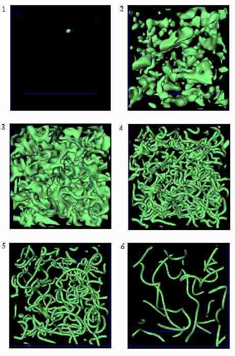
FIG. 1.: String network formation in the Abelian-Higgs model using gradient flow (diffusive) evolution. Given random initial phases, a symmetry-breaking phase transition occurs, strings form and then begin to evolve in a scale-invariant manner (the correlation length is $L\propto t^{1/2}$). This dissipative evolution is used to create the initial configuration for a string network with a specified $L$ for subsequent relativistic evolution.

Other feasible methods to set up the initial network include the imposition of a friction term in the second-order evolution equations, or alternating dissipative evolution with full dynamic evolution. However, using gradient flow ensured that the density of background radiation was minimal at a fixed inter-string spacing. In particular, it gave greater confidence in our subsequent discussion when we were able to eliminate friction as a primary network decay mechanism. As an aside, we note that the evolution of the network during gradient flow, as shown in Fig. 1, was consistent with a scaling law in which the correlation length grew as $L\propto t^{1/2}$ and the velocity decayed as $v\propto t^{-1/2}$. This scaling law is well-known from condensed matter physics and also predicted in this context in the velocity-dependent one-scale model [5] (see later).

After creating the initial configuration through gradient flow, each simulation was evolved using Hamiltonian dynamics as discussed previously. The Gauss constraint was satisfied initially as we start from rest, and was accurately preserved by the equations of motion. The time-steps were chosen to be sufficiently small to ensure the Hamiltonian to be conserved within 1 per cent over the course of each simulation. The choice of spatial lattice spacing was constrained by the desire to meet two conflicting criteria: (i) to simulate a volume which is orders of magnitude larger than the string width, and (ii) to accurately represent the continuum theory. We believe that a physical lattice spacing of $\Delta x=0.5$ ($\beta=1$) is close to the maximum that is reasonable given that at larger spacings there is a significant potential barrier associated with the lattice. Moreover, for oscillating strings of length $\approx 15$ we have observed greatly increased radiation using a larger lattice spacing [14].

There are three important parameters that determine the dynamic range of the simulations, once the size of the simulation grid and the initial physical separation of the strings have been determined. These are the lattice spacing in co-moving coordinates, and the starting and ending times for the simulations. These are determined by specifying the initial string scaling density $\rho t^{2}/\mu$, and requiring, at the end of the simulation, that the physical lattice spacing is 0.5, and that the causal horizon has just propagated to extend across the simulation box. Of course, for the ‘fat string’ algorithm described above, the string remains a fixed size in comoving coordinates, so the second constraint is circumvented.

B String density and velocity analysis

Here we describe in detail how we analyse the string network positions, lengths and velocities. In summary, to characterise the network configuration at a given point in time we assign positions of zeros of the Higgs field to lattice plaquettes according to the winding of the Higgs phase around each plaquette. This allows us to calculate correlation lengths and loop distribution statistics. When combined with similar data from a nearby time-step we can also estimate the velocity of each string segment. As we shall see, the procedure for calculating the velocities is relatively vulnerable to numerical normalisation errors due to uncertainty in the precise position of the string cores.

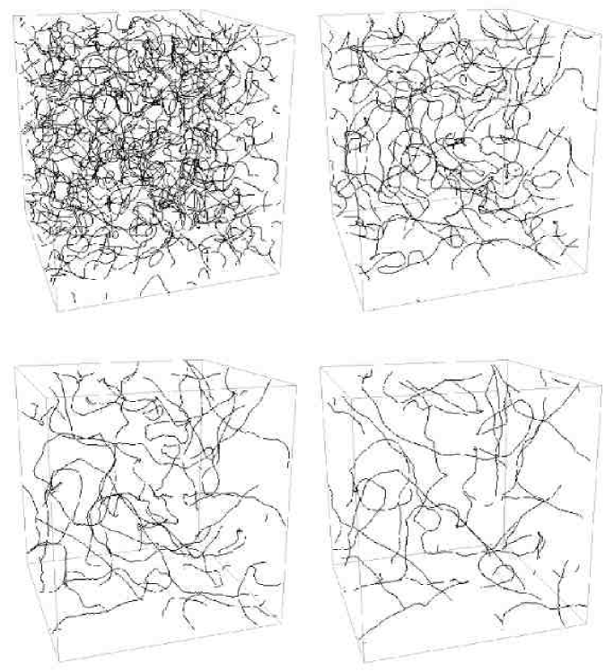
FIG. 2.: String network evolution during the radiation era. Positions for the string cores were found using phase information and the trajectories connected appropriately. Note that lattice discretisation effects have been reduced by smoothing. The respective times for the advancing evolution are the conformal times $t=24,32,40,48$, by which time the horizon is comparable to the box size.

1 Static string length estimation

Positional information for the string was found using the Vachaspati–Vilenkin algorithms as implemented in the Allen–Shellard Nambu string network code [7]. Instead of the random generation of phases, the Abelian-Higgs field theory simulation phases were input and the trajectories of string zeros approximately reconstructed within the accuracy of the lattice discretisation. These trajectories had several string points assigned for each original lattice spacing, with corners automatically rounded. This lattice assignment, however, necessarily creates straight strings along preferred lattice directions and wiggly strings along diagonals. This is not satisfactory either for estimating the static string length or the string velocities. A subsequent period of smoothing or ‘point-joining’ was undertaken to remove most of these small-scale artifacts on length scales smaller than the actual string width $\delta$, while minimising effects above $\delta$. In practice, it was not difficult to tune the smoothing to end after rapid elimination of most of the ‘wiggliness’, before passing over to a slowly decaying phase. The evolution of an Abelian-Higgs string network using these positional estimators is shown in Fig. 2. Note that the strings still exhibit a small amount of ‘wiggliness’ beyond that inherent in the pixelization of the rendered image.

Given this information about the string positions and trajectories, it was a straightforward matter to analyse the total string length and that of individual loops. In particular, we could separate the network into ‘infinite’ loops stretching across the periodic box and analyse the distribution of small loops. In terms of the static configuration, we believe our prescription for estimating the string length is accurate to of order 10%.

2 String velocity estimation

Obtaining velocity estimates from this positional information proved to be challenging, with the overall normalisation remaining the key uncertainty. However, the importance of attempting this is obvious, with one application being the ability to measure the true invariant string length. This differs from the static string length by an average Lorentz factor $\bar{\gamma}\approx(1-v^{2})^{-1/2}$, where $v$ here is the rms velocity of the network weighted over the covariant string length. The total string energy $E=\mu/L^{2}$ is clearly related to the static string energy $E_{\rm s}$ by the relation

$$E=\bar{\gamma}E_{\rm s}\equiv\mu\bar{\gamma}/L_{\rm s}^{2}\,,$$ (8)

where $L_{\rm s}$ is the static string correlation length apparently used in refs. [10, 15, 16]. Hence, given a typical network velocity of $v\approx 1/\sqrt{2}$, a static analysis will underestimate the true string energy density $\rho$ by 40% and overestimate the correlation length by 20%. Furthermore, the static analysis of refs. [15, 16] did not measure actual string trajectories, but rather the proportion of the numerical volume above a particular threshold potential energy. By comparing with a static string profile, an estimate of the string length was made. This appears, however, to neglect a further Lorentz factor since the string cross-section is Lorentz contracted in the direction transverse to its motion. Our expectation of a difference of a factor of two between our density estimates and those of ref. [15] is borne out (refer to the global strings analysis later).

Apart from the overall density normalisation, a static analysis cannot satisfactorily probe the initial relaxation when the velocity is rising from zero to its scaling value. Given the severely restricted dynamic range possible in field theory simulations, this initial relaxation is up to 30% of the total time period available. Both these reasons, then, compel us to make the first attempt to calculate network velocities.

String velocities were estimated by comparing positional information from two simulations with a small temporal separation $\Delta t$, but sufficient to ensure that strings have on average moved more than one lattice spacing $v\Delta t\gtrsim d$. For each individual string point $i$ in one simulation, we undertake an exhaustive search for the nearest two strings points in the second simulation. This is achieved with a radix search implemented in the Nambu code [7] which is of order $N\log N$, where $N$ is the number of string points. Having found the nearest points we connect them with a straight line and find the perpendicular distance $d_{i}$ to the original point. If this distance is such that there could be no causal relationship we reject that point (for example, if a small loop has disappeared during $\Delta t$), otherwise we accept this velocity estimate $v_{i}=d/\Delta t$. We continue iterating over all string points to find the average root mean square velocity $v$ for the whole string network.

This velocity is a non-trivial statistical estimate which, because of lattice discretisation effects, only converges in the limit of measuring many random string positions and orientations. To test the reliability of the method we generated field phase information for a randomly oriented straight string with a given speed $v$ and showed convergence was adequate for $N\gtrsim 1000$ realizations. However, at each velocity there is a systematic offset between the measured rms velocity $v_{\rm m}$ and the true rms velocity $v$. These corrections are important, for example, at small velocities where jumps between discrete lattice centres tend to overestimate the velocities, but there are also systematic effects at high velocity. A comparison of the inferred velocity from an ensemble of moving straight line segments demonstrated the efficacy of this algorithm for estimating the true string velocity in this idealised case (refer to Fig. 3). This was also the case for large circular rings with a typical correlation length found in the field theory simulations. However, for very small rings (at about 1/3 the typical correlation length) the diagnostic underestimated high velocities, thus respresenting a shortcoming for highly curved regions on the string network. The estimated velocity for an admixture of equal numbers of large rings with the correlation length ($L=7.5$) and small rings ($L=2.5$) illustrates this effect in Fig. 3.

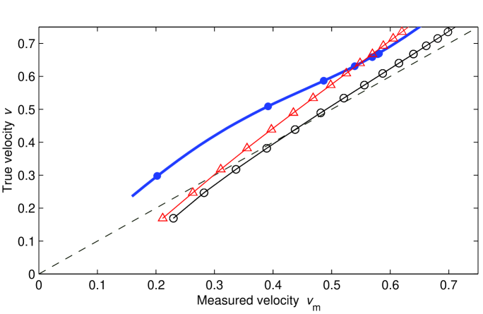
FIG. 3.: Correction to the measured velocity required for the velocity-position diagnostic to obtain the true velocity (solid blue line). This data represents the velocity inferred from the growth in the kinetic energy for an initially static network (see Fig. 4). Tests of the diagnostic for a distribution of straight string segments (circles) showed almost direct proportionality, whereas idealized small and large rings (red triangles) also underestimated the true velocity.

Given these geometrical effects which are not easily quantifiable in a complex string network, we sought an unambiguous normalisation for our velocity diagnostic. This only proved possible by a direct comparison with the overall velocity inferred from the kinetic energy of the full field theory simulations in flat space. During the first few time steps as the initially static string configuration begins to accelerate and move relativistically, the rapid rise in the kinetic energy is due primarily to string motion. Although some radiation will be produced, it is absent in the initial conditions and there is insufficient time for this to be produced in quantity. The proportion of the total energy in this kinetic energy is shown for a large-scale flat space simulation in Fig. 4 (the red dashed line); the initial correlation length is $L=7.5$. Consistent with the rise in the kinetic energy being due to string motion, initially there is almost no change in the overall invariant length of the string network. Plotted as a solid blue line in Fig. 4 is the velocity inferred from modelling the kinetic energy as a change in the string Lorentz factor. This should be valid up to about $t\lesssim L=7.5$, but only a crude upper bound thereafter. By comparing our velocity estimator which uses positional information from the string cores, we can hope to normalise it correctly for a general network configuration. The rescaling shown is about 15% higher than the straight string normalisation discussed above. It yields results consistent with the expected $v\approx 1/\sqrt{2}$ for flat space networks and we believe to be accurate within a 10% range. However, we cannot exclude at this stage the possibility that the velocities quoted in what follows are slightly overestimated (or, less likely, underestimated). There may be unexplored physical mechanisms which can systematically reduce velocities on the small-scales probed by the present simulations.

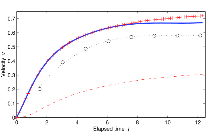
FIG. 4.: The string velocity (solid blue line) inferred from the growth in kinetic energy of a network field theory simulation in flat space (shown as red ’$+$’ data points). The actual proportion of kinetic energy relative to the total energy is the red dashed line. The raw velocity diagnostic before normalisation (circular data points) underestimates the true rms network velocity by about 15%.

C Flat space networks

The growth of the correlation length $L$ for flat space simulations, along with the corresponding rms velocity, is illustrated in Fig. 5. All simulations, which included grid sizes up to $400^{3}$, were halted when the horizon size reached half the box-size. The solid lines in Fig. 5 represent the true correlation length obtained from the total string energy $L=(E/\mu)^{-1/2}$, whereas the dotted lines are the static correlation length $L_{\rm s}$ from 8. This latter diagnostic, employed in [10], gives much more linear initial growth and is consistent with their results. However, it is clear from the velocity-dependent $L$, that the early evolution can be interpreted as primarily due to the acceleration of the initially static network rather than the immediate onset of a decay mechanism capable of reducing the invariant string length.

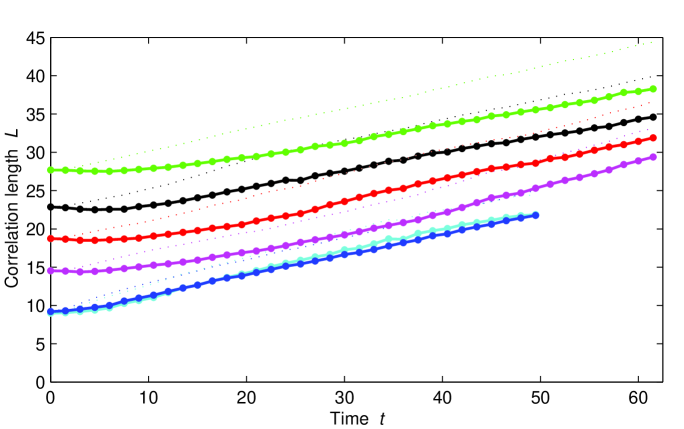
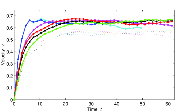
FIG. 5.: Flat spacetime simulation results for a series of simulations with a grid size of $250^{3}$ or above. The top panel shows the spatial correlation length $L$ as a function of time. The dotted lines give the static correlation length $L_{\rm s}$ inferred from the static string density, rather than the total invariant string length used for $L$. The lower panel shows the corresponding average rms velocity $v$ as a function of time (with the same colour coding). The dotted lines give the raw velocity before applying the velocity corrections plotted in Fig. 3.

For higher initial densities than those plotted in Fig. 5 there were some deviations from asymptotic linearity probably due to the effect of background friction on string motion (this may be evident in the bottom two curves with the highest string densities). The asymptotic slopes of the correlation lengths yield the approximate scaling law

$$L=0.23(\pm 0.05)t\,.$$ (9)

Remarkably, this is close to the result $L=0.27(\pm 0.05)$ quoted for the Smith–Vilenkin simulations of Nambu networks in [17]. Our result is consistent to the directly comparable field theory simulations of [10], if the results from their static analysis $L_{\rm s}=(0.27$–$0.34)t$ are divided by the square root of the average Lorentz factor, $\bar{\gamma}\approx 1.4$. The initial brief burst of growth in the correlation length seen for several runs in [10] is not observed in our simulations and may arise from the different procedures used to set up the initial network configurations. (The deviations from linearity seen in their largest run (see Fig. 1 in [10]) appears to be due to the use of a larger lattice spacing for which numerical friction becomes significant.)

The approach to scaling for the velocities can be observed in the lower panel of Fig. 5. The timescale for this process was rapid and roughly inversely proportional to the initial correlation length. The asymptotic values for the different simulations were remarkably consistent, that is, approximately

$$v=0.67(\pm 0.05)\,.$$ (10)

This velocity is consistent, within our conservative error estimates, with naive expectations for a flat space network, that is, $v=1/\sqrt{2}$. As expected, the relaxation time of the velocity towards its asymptotic value was roughly proportional to the initial correlation length (compare upper and lower panels). The very rapid over-relaxation for the smallest correlation length was probably due to additional accelerations from inter-string forces (which have an exponential fall-off at large distances).

D Radiation era string networks

We have performed a very extensive series of network simulations in an expanding universe during the radiation-dominated era $a\propto t^{1/2}$. Simulation results for the relative energy density $\zeta\equiv\rho t^{2}/\mu$ and the rms velocity $v$ are given in Fig. 6. Small bracketing simulations are shown in cyan, with larger simulations ($320^{3}$ or above) in blue. A diamond indicates where the horizon size grows to half the box size. Because of the consistency of the subsequent evolution we continue to plot it, but we note that any analysis of these results must be performed before this causal threshold is crossed. In addition, we have performed a series of runs using the ‘fat string’ algorithms discussed earlier. The purpose of this was to check the relative accuracy of the two methods, rather than to exploit the extra dynamic range that the ‘fat string’ method offers. In this case, small bracketing simulations are plotted in magenta, while the larger simulations (again grids of $320^{3}$ or above) are shown in red. There is surprising consistency between the two methods with the biggest differences emerging in the late-time evolution of the velocities which, in turn, influences the energy density. As we shall discuss, this is the regime in which the resolution of simulations with a physical string width becomes progressively poorer.

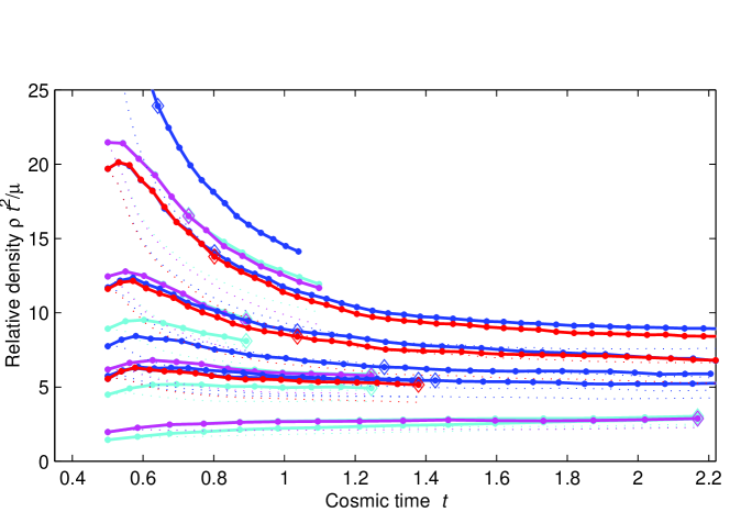
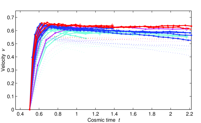
FIG. 6.: Radiation era simulation results: The upper panel shows the relative density for string networks in the radiation era converging towards a ‘scaling’ asymptotic value. The simulations plotted in blue are large (over $320^{3}$) high resolution simulations using the true physical equations of motion. These are bracketed by smaller simulations plotted in cyan. The simulations plotted in red are also large, but evolve the strings using the ‘fat string’ algorithm and these are bracketed by small runs plotted in magenta. The dotted lines shows the string density from a static analysis, that is, neglecting the Lorentz factor due to string velocities. The lower panel shows the average rms velocity $v$ for radiation era strings as a function of cosmic time for the series of simulations described above (using the same colour coding). The dotted lines show the raw measured velocity before it is normalised. Note the long term decline of velocities for defects of fixed physical size (blue).

The asymptotic values of the relative energy density and the velocity were approximately

$$\zeta\equiv\rho t^{2}/\mu=6(\pm 2)\,,\qquad v=0.63(\pm 0.05)\,.$$ (11)

The density is considerably lower than that found in high resolution Nambu simulations for which $\zeta=13(\pm 2)$ [6, 7], but the velocity $v=0.66$ is consistent within the uncertainties. There is, however, a remarkable qualitative concordance in the approach to scaling as well as the initial relaxation. The reason for the lower density, such as the restricted dynamic range and absence of small-scale structure in these field theory simulations, will be discussed when we consider the analytic modelling of these results in the next section.

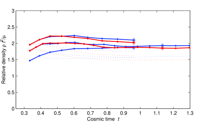
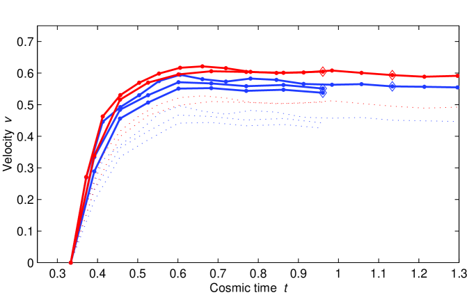
FIG. 7.: Matter era simulation results: The upper panel shows the relative density for string networks in the matter era. The large simulations plotted in blue use the true physical equations of motion, while those plotted in red use the ‘fat string’ algorithm. The lower panel shows the rms string velocity $v$ as a function of cosmic time in the matter era (using the same colour coding as above).

E Matter era string networks

Matter era simulations shown in Figs. 7 were not studied in great detail, except to broadly bracket the apparent scaling value. Combining the simulations we suggest approximate asymptotic values for the relative density and the rms velocity of

$$\zeta=2.0(\pm 0.5)\,,\qquad v=0.57(\pm 0.05)\,.$$ (12)

Again, this density is roughly half that found in high resolution simulations for Nambu networks where $\zeta=3.5(\pm 1)$, but the velocity is again consistent with $v=0.58$–$0.61$ [6, 7]. Regardless of the overall velocity normalisation, the relative velocities for flat space, radiation and matter eras were found to be in the ratios $1.0:0.93:0.83$ which is remarkably consistent with Nambu simulation ratios $1.0:0.94:0.85$. Clearly, Hubble damping is acting on the extended field theory vortex-strings in a similar manner to the one-dimensional Nambu strings.

With the rapid expansion occurring in the matter era, the defect width shrinks very quickly on a comoving grid and so the effective dynamic range of field theory simulations is severely restricted. After reaching the threshold where the defect width and lattice spacing were comparable, numerical accuracy declined dramatically and the velocity plummeted towards zero. In this respect, the ‘fat string’ algorithm fared very much better (plotted in red) showing no sign of the initial decline in velocities evident in simulations solving the true physical equations of motion.

F Global string networks

Global strings provide an interesting contrast to gauged strings because they are known to be strongly radiating, especially on the small scales probed by these simulations. As a further independent check on our work, in [15, 16] global string networks have also been simulated in both matter and radiation eras. Here, we study global strings using the same Abelian-Higgs code but with the couplings altered appropriately. The relative scaling density and velocity were found to be, respectively (refer to Figs. 8),

$$\zeta=2.0(\pm 0.5)\,,\qquad v=0.68(\pm 0.05)\,.$$ (13)

(Note that we use the defects of fixed physical width (blue) to estimate the velocity.) We believe this result for $\zeta$ is consistent with the lower result $\zeta=0.9$–$1.3$ quoted in ref.[15] because the two Lorentz factor corrections to their static analysis (discussed previously), would make the total invariant string density higher by a factor of two.

With only about 8 global strings crossing each horizon volume, this is a dramatically lower density than the 24 strings observed in the local gauged case (and the 50 strings seen in the Nambu simulations). Clearly, the global strings, through their coupling to the massless Goldstone boson, have available a much more effective energy loss mechanism on these scales than local strings which only couple to massive fields. Despite this fact, however, radiation back-reaction effects do not reduce the average rms string velocity, instead it appears to be systematically higher than the local case. This indicates that the strong long-range interactions between global strings are playing an important role in accelerating the network dynamics.

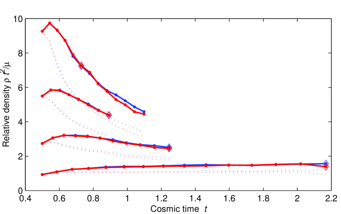
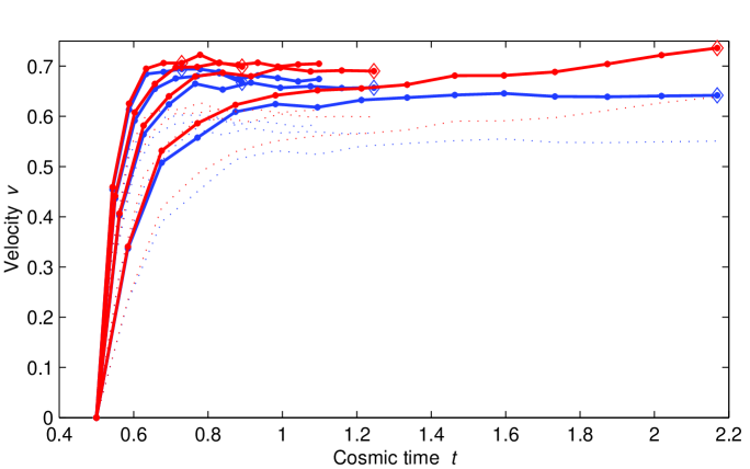
FIG. 8.: Global string simulations in the radiation era: The upper panel shows relative density for global string networks in the radiation era. The large simulations plotted in blue use the true physical equations of motion, while those plotted in red use the ‘fat string’ algorithm. The lower panel shows the average rms velocity $v$ as a function of time for global strings in the radiation era (using the same colour coding as above). Note the diverging velocities for the true (blue) and ‘fat’ (red) global strings.

Finally, we note that the ‘fat string’ algorithm does not appear to mimic the true string dynamics as effectively in the global case (compare the red velocity curves in Fig. 8 with the radiation era local strings, Fig. 6). The physical and ‘fat string’ velocities diverge significantly even when the numerical evolution should remain accurate (that is, before horizon crossing of the box). An important physical effect mitigates against the accuracy of the ‘fat string’ algorithm in the global case. The string energy density (and the inter-vortex potential) has a logarithmic term, $\mu\propto\ln(L/\delta)$, with a width cutoff $\delta$ which continues to grow in this case. This enlarged cutoff $\delta$ implies a lower effective mass and so the string will accelerate more rapidly under the long-range inter-string forces present, and it will also radiate its energy more efficiently.

G Efficacy of the ‘fat string’ algorithm

Summarising our previous discussions, we conclude that our new ‘fat string’ algorithm for local strings in an expanding universe, appears to closely replicate the averaged properties of true string network dynamics. Both the string densities and velocities were in good agreement over the limited dynamic range available to this study. This encourages further application of this method to field theory simulations of local strings in an expanding background, thereby accessing much larger dynamic ranges. However, the detailed implications of the ‘fat string’ algorithm deserve further study, especially for the evolution of the Hamiltonian, the propagation of massive radiation, and the emergence of small-scale structure on strings. As we have also seen, the ‘fat string’ algorithm for global strings fared satisfactorily, but did not reproduce string velocities as successfully. It does not provide a very precise quantitative representation of global string evolution over the small dynamic ranges probed by these simulations, let alone those required to make accurate cosmological predictions.

III Analytic modelling of network evolution

A The velocity-dependent one-scale model

The velocity-dependent one-scale (VOS) model has been described in considerable detail elsewhere [18, 5, 19, 20], so here we limit ourselves to a brief discussion, highlighting the features that will be important for what follows. This generalized ‘one-scale’ model [4], aims to describe the general evolutionary properties of the string network through the behaviour of a small number of averaged or ‘macroscopic’ quantities, namely its energy $E$ and rms velocity $v$ defined respectively by

$$E=\mu a(\tau)\int\epsilon d\sigma\,,\qquad v^{2}=\frac{\int{\dot{\bf x}}^{2}\epsilon d\sigma}{\int\epsilon d\sigma}\,,$$ (14)

where the string trajectory ${\bf x}(\sigma,t)$ is parametrised by the world-sheet coordinates $\sigma$ and $t$ and the ‘energy density’ $\epsilon(\sigma,t)$ gives the string length per unit $\sigma$ along the string. For coherence, here, we summarise the main points of the original ‘one-scale’ model in preparation for the new ingredients of the VOS model.

The long string network is a Brownian random walk on large scales and can be characterised by a correlation length $L$. This can be used to replace the energy $E=\rho V$ in long strings in our averaged description, that is,

$$\rho_{\infty}\equiv\frac{\mu}{L^{2}}\,.$$ (15)

A phenomenological term must then be included to account for the loss of energy from long strings by the production of loops, which are much smaller than $L$. A ‘loop chopping efficiency’ parameter $\tilde{c}$ is introduced to characterise this loop production as

$$\left(\frac{d\rho_{\infty}}{dt}\right)_{\rm to\ loops}={\tilde{c}}v_{\infty}\frac{\rho_{\infty}}{L}\,.$$ (16)

In this approximation, we would expect the loop parameter $\tilde{c}$ to remain constant irrespective of the cosmic regime, because it is multiplied by factors which determine the string network self-interaction rate.

From the microscopic string equations of motion, one can then average to derive the evolution equation for the correlation length $L$,

$$2\frac{dL}{dt}=2HL(1+{v_{\infty}^{2}})+\frac{L}{\ell_{\rm f}}{v_{\infty}^{2}}+{\tilde{c}}v_{\infty}\,,$$ (17)

where $H$ is the Hubble parameter and $\ell_{\rm f}$ is a friction damping length scale. The first term in (17) is due to the stretching of the network by the Hubble expansion which is modulated by the redshifting of the string velocity. The second term is due to frictional interactions by a high density of background particles scattering off the strings. The friction length scale $\ell_{\rm f}$ (defined in [18]) typically depends on the background temperature as $\ell_{\rm f}\approx{\cal O}(1)\mu T^{-3}$, so that it grows with the scale factor as $a^{3}$ and it will become irrelevant at late times. It proves easiest (and physically clearer) to characterise this friction term by a parameter $\theta$ which measures the initial ratio of the damping terms due to friction and expansion. In the case of flat spacetime, however, this friction length scale will be a constant, and hence the effect of this term, if at all relevant, can not be neglected at late times.

The effect of massless radiation on the long-string network can be included in the evolution equation for the correlation length (17) in the same way as previously achieved for the evolution of the length of a string loop [5]. Taking for example the typical case of gravitational radiation, one easily finds [20] that the following term can be added to the right-hand side of (17)

$$2\left(\frac{dL}{dt}\right)_{\rm massless}\equiv 8\Sigma v^{6}_{\infty}\,;$$ (18)

Here, $\Sigma$ is a constant which is the long-string counterpart of $\Gamma G\mu$ found for the gravitational decay of string loops ($\Gamma\approx 65$) [1]. We note that a term for Goldstone boson radiation should also take this form, but with a much larger coefficient $\Sigma$ than for gravitational radiation [21]. For the radiation of massive particles (mass $m$) we expect the above term to be exponentially suppressed (or similar) for correlation lengths well beyond an appropriate inverse mass-scale $L_{\rm d}\sim m^{-1}$. Hence, we can introduce an analogous phenomenological term to describe it:

$$2\left(\frac{dL}{dt}\right)_{\rm massive}\equiv 8\Sigma v^{6}_{\infty}\exp\left(-\frac{L}{L_{\rm d}}\right)\,.$$ (19)

One can also derive an evolution equation for the long string velocity with only a little more than Newton’s second law

$$\frac{dv_{\infty}}{dt}=\left(1-{v^{2}_{\infty}}\right)\left[\frac{k}{L}-\left(2H+\frac{1}{\ell_{\rm f}}\right)v_{\infty}\right]\,,$$ (20)

where $k$ is called the ‘momentum parameter’. The first term is the acceleration due to the curvature of the strings and the second damping term is from both the expansion and background friction. The parameter $k$ is defined by

$$k\equiv\frac{\langle(1-{\dot{\bf x}^{2}})({\dot{\bf x}}\cdot{\bf u})\rangle}{v(1-v^{2})}\,,$$ (21)

with ${\dot{\bf x}}$ the microscopic string velocity and ${\bf u}$ a unit vector parallel to the curvature radius vector. An accurate ansatz for $k$ can be derived and justified—see [20]. For strings in near vacuum, we are interested in the relativistic regime for which a sufficiently precise phenomenological form is

$$k_{\rm rel}(v)=\frac{2\sqrt{2}}{\pi}\;\frac{1-8v^{6}}{1+8v^{6}}\,.$$ (22)

We note that in the opposite friction-dominated case, the non-relativistic limit is $k_{\rm nr}(v)={2\sqrt{2}}/{\pi}$. The non-relativistic scaling law predicted is then $L\propto t^{1/2}$ and $v\propto t^{-1/2}$ [5].

The VOS model model has been extensively compared with the results of numerical simulations [6, 7, 22] and shown to provide a good fit to the large-scale properties of a string network. In particular, it matches well the evolution between asymptotic regimes as a network passes through the matter–radiation transition. Comparisons with numerical simulations confirm the constancy of the only free parameter, the loop chopping efficiency $\tilde{c}$, and fix its value in the expanding universe to be [22]

$$\tilde{c}=0.23\pm 0.04\,,$$ (23)

and, in Minkowski space,

$$\tilde{c}=0.57\pm 0.04\,,$$ (24)

that is, about twice as large (we will return to this point below). For a detailed discussion of other regimes of applicability of this model (such as open and $\Lambda$-universes), as well as an analysis of its various scaling solutions, refer to [20].

In what follows, we will use this model to fit the numerical simulations described previously. We will concentrate on trying to identify which of the different dynamical mechanisms (loop production, friction or radiation) is dominant for the evolution of the network. In doing so we will look for distinguishing features that differentiate between these mechanisms. For example, friction reduces string velocities, whereas loop production and radiative effects exhibit different behaviours in their initial relaxation due to their different dependence on the velocity $v$. Note that we will only endeavour to fit data before the horizon crosses the numerical box, that is, for times prior to the diamonds plotted in the expanding universe simulations.

B Flat space modelling

We start by considering the effect of friction alone, that is, we hypothesise that the initial gradient flow actually leaves behind a substantial background between the relaxed strings in the initial configuration. Friction has two competing effects on the string density (or correlation length). On one hand, increasing the friction parameter $\theta$ will make $L$ grow faster, but on the other hand it will also decrease the string velocity $v$. Given that the friction term is proportional to $Lv^{2}$, there will be an ‘optimal’ value of $\theta$ that will provide a best-fit for the string density. We find that this is near $\theta\sim 0.1$, and we compare with simulations in Fig. 9. We can see that it is a very poor fit, primarily because the velocities are too low and their asymptotic values differentiate (unlike the consistent asymptote of the simulation data). For this reason, we can rule out friction as an important influence on the network dynamics, giving us greater confidence in the effectiveness of the initial gradient flow in creating a negligible background.

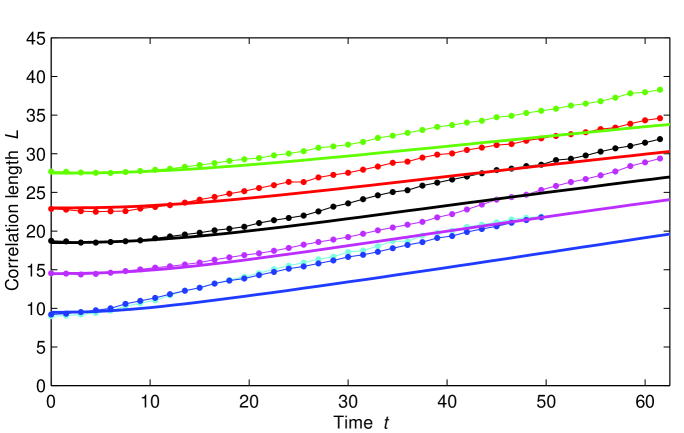
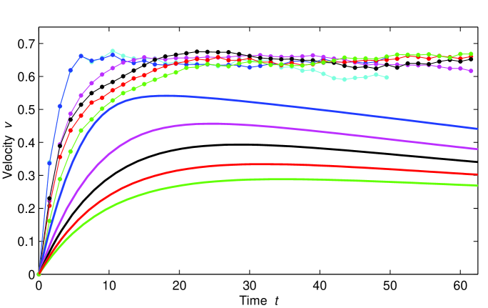
FIG. 9.: Friction-dominated strings in flat space. The best fit VOS model with friction only $\theta=0.1$ (solid lines), is compared to the flat space simulation data (data points). These fits are very poor, especially for the velocities, and rule out friction as a dominant dynamical effect in these string network simulations.

We next consider the effect of radiation in the VOS model, with a best-fit shown in the upper panel of Fig. 10 for the radiation parameter $\Sigma=0.8$ ($L_{\rm d}\rightarrow\infty$). This is motivated by the ‘scale-invariant massive radiation’ scenario proposed in ref. [10] and in which massive particle emission is not cut-off beyond some inverse mass-scale ($L_{\rm d}\rightarrow\infty$). Although our previous work suggests that massive radiation cannot be produced in this manner [12], there is a reasonable fit in Fig. 10 to the flat space simulation data, implying we cannot rule out this possibility on these grounds alone. However, we note the particular parameter choice with $\Sigma=0.8$ and will confront the model later with expanding universe data.

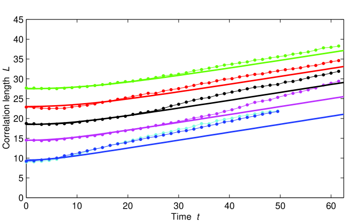
FIG. 10.: Possible energy loss mechanisms for flat space string networks showing analytic fits for a ‘scale-invariant massive radiation’ scenario (upper panel) and for the standard loop production model (lower panel). In the upper panel, the VOS model (solid lines) with only ‘massless’ radiation $\Sigma=0.8,L_{\rm d}\rightarrow\infty$, ($\tilde{c}=0$) is a satisfactory fit to the simulation data points. In the lower panel, the best fit (solid lines) for loop production has ${\tilde{c}}=0.57$ ($\Sigma=0$) which corresponds to the value also found for flat space Nambu networks. There is some evidence of small deviations from the simulated data (solid lines) for small initial correlation lengths $L$.

Next we consider the case of loop production only, see the lower panel of Fig. 10. Here the best fit is provided by ${\tilde{c}}=0.57\pm 0.05$. Note that this is precisely the same value that was found in flat spacetime Nambu string simulations [20, 22] (refer also to [17]). We can see that the fit is quite good for initial conditions corresponding to high values of the correlation length, and that it gets comparatively less accurate as this decreases. This is what one would expect if there is an extra, relatively small initial contribution from massive radiation.

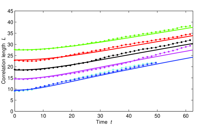
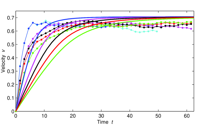
FIG. 11.: Loop production model with some massive radiation for flat space string networks. This shows the very good fit between simulated strings (solid lines) and the VOS model (dashed lines) assuming loop production (${\tilde{c}}=0.57$) with some massive radiation ($\Sigma=0.5,~{}L_{\rm d}=4\pi$).

In Fig. 11 we show an improved fit where we have added a massive radiation term of strength $\Sigma=0.5$ and the exponential cut-off value $L_{\rm d}=4\pi$ (motivated by our study of massive radiation from strings [14]). This choice implies that loop production is predominant throughout this simulation but is supplemented with a brief initial burst of massive radiation if the correlation length is sufficiently small (refer to (19)). One can readily observe that that this provides a very good fit to the correlation lengths and to the asymptotic velocities. (Indeed, this is our overall ‘best fit’ model in that it is the parameter choice which provides good agreement for all thirty different local string simulations, whether in flat space or an expanding universe.) Here, we appear to have found a rather encouraging correspondence between the present flat spacetime field theory simulations, analogous Nambu simulations and the analytic VOS model.

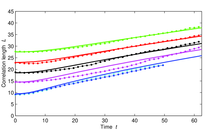
FIG. 12.: An alternative fit to the flat space simulation data using a ‘corrected’ velocity VOS model with the radius of curvature $R=L/2$ (see text). Here, the parameter choice is ${\tilde{c}}=0.45$, $\Sigma=1$ and $L_{\rm d}=4\pi$.

C An alternative velocity fit

The one shortcoming of the correspondence between the simulation data and the VOS model is in the fast initial rise of the velocities, before they begin to approach their asymptotic values. This is not entirely surprising, because the initial conditions can be chosen such that the string curvature radius $R$ and the string correlation length $L$ (as defined in (15)) are significantly different; the VOS model assumes that they are comparable. In principle, a phenomenological term could incorporate this effect by modifying the $k/L$ term in the VOS model (20). We find that an initial ratio of $L\sim 2R$ would significantly improve the early-time velocity fits. The best-fit for the flat spacetime simulations is shown for comparison in Fig. 12; note that the best-fit model parameters are now ${\tilde{c}}=0.45$ and $\Sigma=1$. Even though this improves the very early time fits (notably for the velocities), it does not do as well in terms of key asymptotics. Indeed, to obtain a satisfactory fit in the expanding case we require a rather different parameter choice (for radiation $\tilde{c}=0.4$, $\Sigma=0.75$).

Interestingly, this factor of two correction between the curvature radius $R$ and correlation length $L$ is confirmed when they are measured directly from the simulation initial conditions. However, as the simulation evolves, the initial conditions are erased and the two length scales become increasingly similar. Thus there is nothing ‘fundamental’ about this initial ratio of 2—it is related to the particular way in which the network is generated using diffusive evolution. Other initial conditions, such as those from the Vachaspati-Vilenkin algorithm, produce statistically different networks which would have different $L/R$ ratios (in this case 1.4), which evolve towards unity in a different way. We, therefore, disregard the transient effect of the initial conditions and continue with the unmodified VOS model because of its success in matching important asymptotic results in both flat and expanding backgrounds.

We note also that the VOS model is missing any small-scale physics beyond the accelerations due to the string curvature. Inter-string forces are significant for the small string separations inherent in our particular initial conditions. The strongest evidence for their influence has already been discussed for global strings.

D Expanding universe modelling

We begin for the radiation era data by considering the individual effects of massive radiation and loop production, refer to Fig. 13. The ‘scale-invariant massive radiation’ scenario is shown in the top panel; the best-fit value $\Sigma=0.8$ (assuming $L_{\rm d}\rightarrow\infty$), is the same as in the flat spacetime case. However the fit to the energy density appears to be rather poor, primarily because the initial relaxation is too slow due to the inherent velocity dependence of the radiation terms in (19). It appears that the ‘scale-invariant massive radiation’ scenario of ref. [10] does not provide an adequate description of the actual network dynamics.

In the bottom panel of Fig. 13 we have plotted the model predictions for both ${\tilde{c}}=0.57$ (appropriate in flat spacetime for both Abelian-Higgs and Nambu string networks) and for ${\tilde{c}}=0.23$, which was found to provide the best fit for both radiation and matter era Nambu simulations[20, 22]. We find that ${\tilde{c}}=0.57$ provides a very reasonable fit (solid lines), whereas ${\tilde{c}}=0.23$ clearly does not (dotted lines). This is, however, not entirely unexpected given that Nambu network simulations can probe a much wider range of length scales below the correlation length, thus allowing small-scale ‘wiggles’ to build up on those scales. In other words, no currently available field theory simulation has a spatial resolution or dynamic range sufficiently large to allow for the build-up of small-scale structures on the strings.

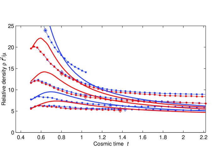
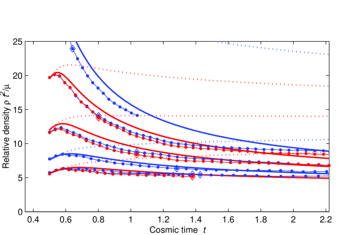
FIG. 13.: Top panel: ‘Scale-invariant massive radiation’ scenario for radiation era strings. The best fit VOS model (solid lines) with ‘scale-invariant massive radiation’ only, $\Sigma=0.8,L_{\rm d}\rightarrow\infty$ ($\tilde{c}=0$) produces a poor initial fit to the simulation data (red and blue lines). Bottom panel: Loop production model in the radiation era. The overall best fit VOS model (solid lines) has the same loop production coefficient ${\tilde{c}}=0.57$ ($\Sigma=0$) as flat space simulations. Using ${\tilde{c}}=0.23$ found for radiation era Nambu networks produces a poor fit (dotted lines) to the simulated data.

The value of ${\tilde{c}}=0.57$ can therefore be regarded as a ‘bare’ loop chopping efficiency, while ${\tilde{c}}=0.23$ can be interpreted as a ‘renormalised’ one. Note that this is also consistent with the fact that Nambu simulations in the expanding case somewhat surprisingly possess much more small-scale structure than corresponding flat spacetime strings (for example, as quantified by the fractal properties of each network) [20, 22]. Note also that the approximate factor of two difference between the two loop production rates may be related to the well-known result that the ‘renormalised’ and ‘bare’ string mass per unit length differ by about a factor of two in radiation era Nambu simulations [6, 7, 22]. We will discuss these issues further in the next section.

In Fig. 14, we provide what appears to be an excellent fit to the radiation era data using exactly the same model parameters as in flat space. The model is loop production supplemented with some massive radiation again using ${\tilde{c}}=0.57$, $\Sigma=0.5$. This surprisingly good fit implies that we have found remarkable consistency between the flat spacetime and radiation era simulations using what can be described as the standard picture of string network evolution.

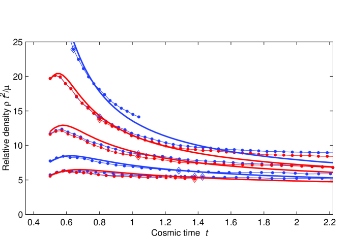
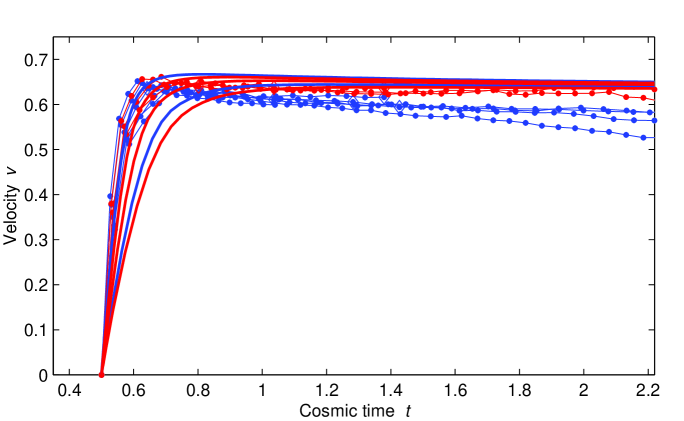
FIG. 14.: Radiation era simulation results fitted with our standard ‘best fit’ VOS model, that is, loop production model with some massive radiation. This excellent fit has the same parameters as for the flat space results in Fig. (11), that is, ${\tilde{c}}=0.57$, $\Sigma=0.5$, and $L_{\rm d}=4\pi$ (appropriately rescaled). Note, as in other figures, that comparisons must be made before the horizon crosses the numerical box (marked with a diamond).

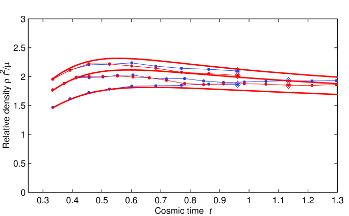
FIG. 15.: Analytic modelling of matter era string simulations. Here we find a good fit to the simulated data points using the VOS model (solid lines) with loop production and some massive radiation using radiation era/flat space parameters (${\tilde{c}}=0.57,\,\Sigma=0.5$, and $L_{\rm d}=4\pi$).

For completeness we also compare the VOS model with the limited simulation data we currently have available for string networks in the matter era. Fig. 15 illustrates a very satisfactory correspondence between the data and the loop production/massive radiation description which does so well in the radiation era and flat space (again ${\tilde{c}}=0.57$, $\Sigma=0.5$).

E Global string modelling

Finally, in Fig. 16 we show an analogous plot for global string networks in the radiation and matter eras. Here we retain the same loop chopping efficiency, ${\tilde{c}}=0.57$, but we require a much larger radiation coefficient, namely $\Sigma\sim 1.1$, to obtain satisfactory correspondence (in this case the radiation is massless with the radiation damping length $L_{\rm d}\rightarrow\infty$ in (19)). The fits to the string density are very good, but the deviations for the string velocities are slightly worse than for local strings. In passing however, we note that if we had followed the velocity correction procedure outlined above we could obtain an excellent fit for the global string velocities (not just for the very early time evolution, but for the asymptotic behaviour as well), albeit still with different best-fit parameters. This would correspond to incorporating the effect of the strong long-range forces in the VOS model which are clearly important for the small length-scales probed by these simulations.

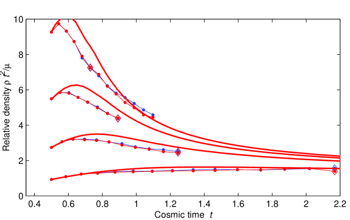
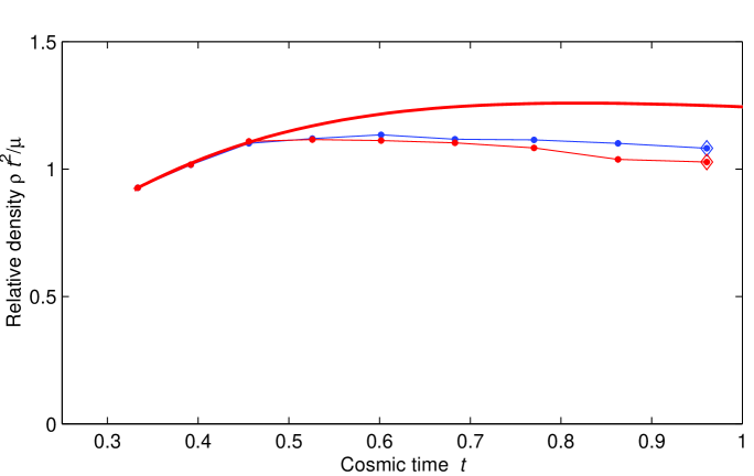
FIG. 16.: Analytic modelling of global strings in the radiation (top) and matter (bottom) eras. A good fit to the simulated data (red lines) was obtained with a VOS model (black lines) with the same loop production as local strings (${\tilde{c}}=0.57$) and the addition of a large massless radiation damping coefficient ($\Sigma=1.1$).

As expected, we can account for the large difference between the local and global string densities through the strong radiative damping of the latter ($\Sigma\sim 1$). The radiation back-reaction equivalent of $\Gamma G\mu$ for the global string is the quantity [21]

$$\kappa=\Gamma/2\pi\ln(L/\delta)\,,$$ (25)

where the average logarithmic cut-off for these simulations is certainly less than $\ln(L/\delta)\lesssim 3$. Using the standard value for loops $\Gamma\approx 65$ as an upper bound, we have $\kappa\gtrsim 2$ which with $\Sigma\approx\kappa$ implies very strong radiative damping for the simulated global strings (especially when compared with $\Gamma G\mu\sim 10^{-4}$ for GUT-scale local strings). We must be extremely careful, therefore, before extrapolating this small global/local string density ratio from these simulations to cosmological scales (for example, as was assumed in [15, 16]). The logarithmic term in (25) for cosmological global strings is much larger, typically with $\ln(L/\delta)\gtrsim 100$. Thus the damping coefficient will fall below $\Sigma\lesssim 0.1$, radiative effects will become perturbative and loop production will dominate, so the VOS model predicts that cosmic local and global strings will actually have very comparable densities. This point illustrates the value of a combined numerical and analytic approach when attempting to describe these complex nonlinear systems in a cosmological context.

F Competing energy loss mechanisms

The analytic modelling up to this point appears to be consistent with the standard picture in which loop production is the primary decay mechanism. It remains, however, to test this phenomenological conclusion directly by measuring the actual energy loss into loops during the simulations. In doing this, however, we face an obvious difficulty which requires a very different treatment of the loop distribution than in the usual ‘one scale’ model. If the standard cosmological picture of loop production is correct, then we know from high resolution Nambu string simulations that the typical loop creation scale $\bar{\ell}$ relative to the horizon is $\alpha\equiv\bar{\ell}/t\lesssim 10^{-3}$ (if gravitational radiation back-reaction sets this limit then $\alpha\sim 10^{-4}$ for GUT-scale strings). The present field theory simulations, however, have a dynamic range which is at least two orders of magnitude poorer, so we cannot realistically hope to probe such small-scale regimes. In consequence, we might be surprised to be able to identify any loops at all in field theory simulations and we certainly would not expect their average creation size $\bar{\ell}$ to ‘scale’ relative to $L$. Instead, our numerical studies suggest that most loops are created with radii comparable to the string thickness, with $\bar{\ell}\sim\pi$ almost constant throughout. Simulation visualisations seem to indicate that most energy is lost via such small loops or ‘proto-loops’, that is, small-scale highly nonlinear, but coherent, regions of energy density (as illustrated in Fig. 17). Consistent with the Nambu simulations, this ‘proto-loop’ production occurs—like small loop formation—in high curvature regions where the strings collapse and become very convoluted [23].

A proportion of these ‘proto-loops’ have sufficient topology to be identified as loops by our numerical diagnostics, so we can estimate the energy loss via this pathway relative to other mechanisms. Because these small loops are comparable to the string thickness, they are strongly self-interacting and can be expected to be self-intersecting. We can infer (and we see this in visual animations) that they annihilate very rapidly, decaying into massive particles almost as fast as allowed by causality. Instead of long-lived non-intersecting loops slowly decaying by gravitational radiation (with typical lifetimes $\tau\gtrsim 10^{-4}\bar{\ell}$), the simulation loops collapse and disappear like a circular loop in only half a period, that is, in a time $\tau\approx\ell/4$. Hence, their time-dependent length, can be described approximately by

$$\ell\approx\ell_{\rm c}-4(t-t_{\rm c})\,,\qquad 0<t-t_{\rm c}<\ell_{\rm c/4}$$ (26)

where the loop creation length and time are $\ell_{\rm c}$ and $t_{\rm c}$. At any one time, then, the string energy loss through this rapid loop decay can be simply approximated by

$$\dot{\rho}_{\infty}\approx-4\mu n_{\ell}\,,$$ (27)

where $n_{\ell}$ is the small loop number density.

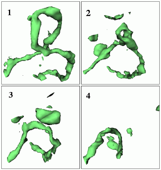
FIG. 17.: Four stages of the formation of ‘proto-loops’ in the field theory simulations: A highly curved region of string (i), collapses to form a nonlinear ‘lump’ in the energy density (ii), which leaves the string (iii) to decay and disappear (iv). This can only happen when the the string’s topological winding inter-commutes or annihilates in this region. Energy density contours are plotted.

For linear scaling to pertain in the ‘one-scale’ model, a dominant energy loss mechanism must behave as $\dot{\rho}_{\infty}\propto\rho_{\infty}/L\propto t^{-3}$ (refer, for example, to (16)). Equating this with the overall small loop decay rate (27), implies that we can achieve scaling with $n_{\ell}\propto t^{-3}$ or, equivalently, with a loop energy density $\rho_{\ell}=\mu\bar{\ell}n_{\ell}\propto t^{-3}\propto\rho/t$ (with $\bar{\ell}$ constant). Thus, with rapidly decaying loops of small constant size, it is possible to maintain network scaling while their relative contribution to the string energy density falls dramatically as $\rho_{\ell}/\rho\propto t^{-1}$. (Contrast this with the standard long-lived loop scenario in which the loop and infinite string densities remain proportional $\rho_{\ell}/\rho_{\infty}\propto{\rm const.}$)

Fig. 18 illustrates the relative small loop contribution to the overall energy density losses throughout a specific flat space simulation, that is, the case with $L_{\rm i}=14.5$ shown in Fig. 5 (magenta line). This is compared with our overall ‘best fit’ VOS model in which loop creation is dominant but with some additional massive radiation. We can observe that the measured loop energy losses grow steadily towards the analytic loop contribution, which for these simulations we assume must include ‘proto-loops’ both with topology and without. We can see that the proportion of loops—the topological ‘proto-loops’—gradually grows to meet or even overtake the analytic loop contribution by the end of the simulation. (Note that this correspondence is qualitative as we do not have a precise measure of the typical small loop energy.)

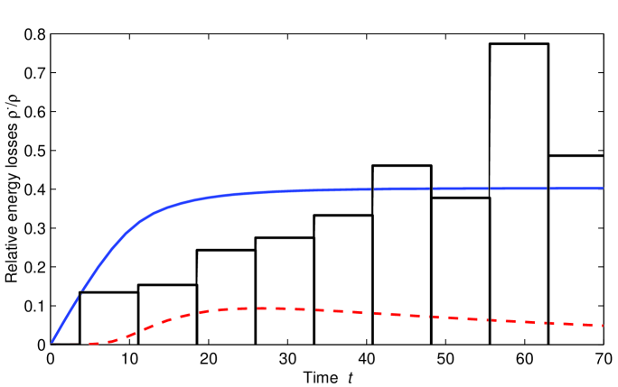
FIG. 18.: The relative contributions of the different components to the overall energy density losses of a flat space string network, as predicted the analytic VOS model for the simulation in Fig. 5 with $L_{\rm i}=14.5$. The best fit parameters are $\tilde{c}=0.57$, $\Sigma=0.5$ and $L_{\rm d}=4\pi$, and shown are loop creation losses (solid blue line) and massive radiation (dashed red line). Superposed onto this figure is a roughly normalised histogram of energy loss into loop production estimated directly from measurements of the time-varying loop density in this particular simulation. It is apparent that the loop energy loss contribution is becoming more important as the simulation progresses.

We surmise that loop/proto-loop production appears to provide a viable explanation for the decay mechanism which maintains the scale-invariant evolution observed in the simulations. However, this discussion is only a small initial step and needs to be made much more quantitative. First, the simple analytic model describing rapidly decaying loops needs to be developed further and, secondly, loop production rates, distributions and decay timescales need to be investigated in much greater detail in large field theory simulations. Nevertheless, it is interesting to speculate about the clear qualitative trend that appears to be evident in Fig. 18. In extrapolating to cosmological scales we increase the ratio of the correlation length to the string width by a further twenty orders of magnitude. It is not unreasonable to expect, therefore, that the loop contribution will become the completely dominant network decay mechanism. As the typical string perturbation length scale grows and is affected by radiative back-reaction, it is again reasonable to suppose that the typical loop creation size will also grow, becoming many orders of magnitude larger than the string thickness. Thus we could conclude that these field theory simulations, once we account for their small dynamic range, can be interpreted as being consistent with the standard picture of long string network evolution via small loop production. Conversely, at the very least, the simulations do not provide compelling evidence that cosmological strings will decay primarily through the direct radiation of ultra-massive particles.

IV Conclusion

We have explored and characterised scale-invariant string network dynamics in numerical field theory simulations for local gauged strings and global strings in flat space and, in an expanding background, in both radiation and matter eras. We have estimated both the typical ‘scaling’ energy density and the rms velocities of the strings for the dynamical ranges currently accessible numerically. We have successfully modelled the density and velocity of these string networks using a simple ‘one scale’ analytic model (the VOS model), describing network decay into small loops, supplemented with some direct massive radiation. We conclude, from these analytic fits and a qualitative examination of loop production, that these results produce an apparently coherent and adequate model for string network evolution. However, this is not to suggest that we have provided a complete or detailed description of the complex nonlinear processes that underlie network evolution on these small scales and many avenues of research remain to be investigated.

An interesting outstanding issue is the close correspondence between the loop creation efficiency $\tilde{c}$ in flat space Nambu simulations and abelian-Higgs simulations in both flat and expanding backgrounds. Field theory simulations do not appear to have sufficient resolution at present to allow for the accumulation of the small-scale structure so evident in expanding universe Nambu simulations. The ‘fat string’ algorithm we have presented can be used to extend the dynamic range of simulations, but the smallest physical scales in this case also grow. Mesh refinement techniques are likely to be necessary in order to make major advances over the present work.

These results have significant cosmological implications. Our expectation is that massive particles will only be produced infrequently in highly nonlinear string regions, such as at cusps and re-connections. The ensuing flux of cosmic rays should be relatively low [24, 25, 26, 27]. It now appears that some estimates of the ensuing cosmic ray flux from direct massive radiation from strings were overly optimistic [10]. This work points to the need for caution in making cosmological extrapolations from small-scale numerical simulations and to the need for further progress understanding string radiation back-reaction.

REFERENCES

- [1] A. Vilenkin and E.P.S. Shellard, Cosmic Strings and Other Topological Defects’, Cambridge University Press (2000).
- [2] M. Hindmarsh and T.W.B. Kibble, Rep. Prog. Phys. 58, 477 (1995).
- [3] H.B. Geyer, Field Theory, Topology and Condensed matter Physics, Springer-Verlag (New York, 1995).
- [4] T.W.B. Kibble, Nucl. Phys. B252, 277 (1985); Erratum: Nucl. Phys. B261, 750 (1986).
- [5] C.J.A.P. Martins and E.P.S. Shellard, Phys. Rev. D54, 2535 (1996) and references therein.
- [6] D.P. Bennett and F.R. Bouchet, Phys. Rev. D41, 2408 (1990).
- [7] B. Allen and E.P.S. Shellard, Phys. Rev. Lett. 64, 119 (1990).
- [8] D. Austin, E.J. Copeland and T.W.B. Kibble, Phys. Rev. D48, 5594 (1993).
- [9] C.J.A.P. Martins and E.P.S. Shellard, in preparation (2001).
- [10] G. Vincent, N. Antunes and M. Hindmarsh, Phys. Rev. Lett. 80, 2277 (1998).
- [11] M. Srednicki and S. Theisen, Phys. Lett. B189, 397 (1987).
- [12] J.N. Moore and E.P.S. Shellard, hep-ph/9808336 (1998).
- [13] K.D. Olum and J.J. Blanco-Pillado, Phys. Rev. Lett. 84, 4288 (2000).
- [14] J.N. Moore and E.P.S. Shellard, in preparation (2001).
- [15] M. Yamaguchi, Phys. Rev. D60, 103511 (1999).
- [16] M. Yamaguchi, J. Yokoyama and M. Kawasaki, Phys. Rev. D61, 061301 (2000).
- [17] G. Vincent, M. Hindmarsh and M. Sakellariadou, Phys. Rev. D56, 637 (1997).
- [18] C.J.A.P. Martins and E.P.S. Shellard, Phys. Rev. D53, 575 (1995).
- [19] C.J.A.P. Martins, Ph.D. Thesis, University of Cambridge (1997).
- [20] C.J.A.P. Martins and E.P.S. Shellard, hep-ph/0003298 (2000).
- [21] R.L. Davis, Phys. Lett. 180B 225 (1986). A. Vilenkin & T. Vachaspati, Phys. Rev. D35, 1138 (1987). R.A. Battye and E.P.S. Shellard, Phys. Rev. Lett. 75, 4354 (1995).
- [22] C.J.A.P. Martins and E.P.S. Shellard, ‘Testing the velocity-dependent one-scale model’, in preparation (2001).
- [23] E.P.S. Shellard and B. Allen, ‘On the evolution of Cosmic Strings’, in ‘The formation and evolution of cosmic strings’, G.W. Gibbons et al., (eds.), Cambridge University Press (1990).
- [24] P. Bhattacharjee and N.C. Rana, Phys. Lett. B246, 265 (1990).
- [25] P. Bhattacharjee and G. Sigl, Phys. Rep. 327, 109 (2000).
- [26] R.J. Protheroe and T. Stanev, Phys. Rep. 77, 3708 (1996).
- [27] V. Berezinsky, P. Blasi and A. Vilenkin, Phys. Rev. D58, 103515 (1998).
- [28] K. J. M. Moriarty, E. Myers and C. Rebbi, Phys. Lett. B207, 411 (1988).
- [29] W.H. Press, B.S. Ryden and D.N. Spergel, Ap. J. 347, 590 (1989).
- [30] B.S. Ryden, W.H. Press and D.N. Spergel, Ap. J. 357, 293 (1990).
- [31] D.N. Spergel, N. Turok, W.H. Press and B.S. Ryden, Phys. Rev. D43, 1038 (1991).
- [32] J.-W. Ye and R. H. Brandenberger, Mod. Phys. Lett. A5, 157 (1990). J.-W., Ye, and R.H. Brandenberger, Nucl. Phys. B346, 149 (1990). B.S. Ryden, Phys. Rev. D43, 1038 (1991).