Inconsistencies in Models
for RHIC and LHC

¹ SUBATECH, Universit de Nantes – IN2P3/CNRS – EMN, Nantes, France
² Moscow State University, Institute of Nuclear Physics, Moscow, Russia
³ Institute f. Kernphysik, Forschungszentrum Karlsruhe, Karlsruhe, Germany
⁴ Physics Department, New York University, New York, USA

^a Invited speaker at the 17th Winter Workshop on Nuclear Dynamics,

March 2001, Park City, USA

Abstract

The interpretation of experimental results at RHIC and in the future also at LHC requires very reliable and realistic models. Considerable effort has been devoted to the development of such models during the past decade, many of them being heavily used in order to analyze data.

It is the purpose of this paper to point out serious inconsistencies in the above-mentioned approaches. We will demonstrate that requiring theoretical self-consistency reduces the freedom in modeling high energy nuclear scattering enormously.

We will introduce a fully self-consistent formulation of the multiple-scattering scheme in the framework of a Gribov-Regge type effective theory. In addition, we develop new computational techniques which allow for the first time a satisfactory solution of the problem in the sense that calculations of observable quantities can be done strictly within a self-consistent formalism.

1 Inconsistencies

With the start of the RHIC program to investigate nucleus-nucleus collisions at very high energies, there is an increasing need of computational tools in order to provide a clear interpretation of the data. The situation is not satisfactory in the sense that there exists a nice theory (QCD) but we are not able to treat nuclear collisions strictly within this framework, and on the other hand there are simple models, which can be applied easily but which have no solid theoretical basis. A good compromise is provided by effective theories, which are not derived from first principles, but which are nevertheless self-consistent and calculable. A candidate seems to be the Gribov-Regge approach, and – being formally quite similar – the eikonalized parton model. Here, however, some inconsistencies occur, which we are going to discuss in the following, before we provide a solution to the problem.

Gribov-Regge theory [1, 2] is by construction a multiple scattering theory. The elementary interactions are realized by complex objects called “Pomerons”, who’s precise nature is not known, and which are therefore simply parameterized, with a couple of parameters to be determined by experiment [3]. Even in hadron-hadron scattering, several of these Pomerons are exchanged in parallel (the cross section for exchanging a given number of Pomerons is called”topological cross section”). Simple formulas can be derived for the (topological) cross sections, expressed in terms of the Pomeron parameters.

In order to calculate exclusive particle production, one needs to know how to share the energy between the individual elementary interactions in case of multiple scattering. We do not want to discuss the different recipes used to do the energy sharing (in particular in Monte Carlo applications). The point is, whatever procedure is used, this is not taken into account in the calculation of cross sections discussed above [4],[5]. So, actually, one is using two different models for cross section calculations and for treating particle production. Taking energy conservation into account in exactly the same way will modify the (topological) cross section results considerably.

Another very unpleasant and unsatisfactory feature of most “recipes” for particle production is the fact, that the second Pomeron and the subsequent ones are treated differently than the first one, although in the above-mentioned formula for the cross section all Pomerons are considered to be identical.

Being another popular approach, the parton model [6] amounts to presenting the partons of projectile and target by momentum distribution functions, $f_{i}$ and $f_{j}$, and calculating inclusive cross sections for the production of parton jets as a convolution of these distribution functions with the elementary parton-parton cross section $d\hat{\sigma}_{ij}/dp_{\perp}^{2}$, where $i,j$ represent parton flavors. This simple factorization formula is the result of cancellations of complicated diagrams and hides therefore the complicated multiple scattering structure of the reaction, which is finally recovered via some unitarization procedure. The latter one makes the approach formally equivalent to the Gribov-Regge one and one therefore encounters the same conceptual problems (see above).

2 A New Self-consistent Approach

As a solution of the above-mentioned problems, we present a new approach which we call “Parton-based Gribov-Regge Theory”: we have a consistent treatment for calculating (topological) cross sections and particle production considering energy conservation in both cases; in addition, we introduce hard processes in a natural way.

The basic guideline of our approach is theoretical consistency. We cannot derive everything from first principles, but we use rigorously the language of field theory to make sure not to violate basic laws of physics, which is easily done in more phenomenological treatments (see discussion above).

Let us first introduce some conventions. We denote elastic two body scattering amplitudes as $T_{2\rightarrow 2}$ and inelastic amplitudes corresponding to the production of some final state $X$ as $T_{2\rightarrow X}$ (see fig. 1).

      

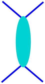
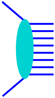
Figure 1: An elastic scattering amplitude $T_{2\rightarrow 2}$ (left) and an inelastic amplitude $T_{2\rightarrow X}$ (right).

As a direct consequence of unitarity on may write the optical theorem $2\mathrm{Im}T_{2\rightarrow 2}=\sum_{x}$$(T_{2\rightarrow X})$$(T_{2\rightarrow X})^{*}$. The right hand side of this equation may be literally presented as a “cut diagram”, where the diagram on one side of the cut is $(T_{2\rightarrow X})$ and on the other side $(T_{2\rightarrow X})^{*}$, as shown in fig. 2.

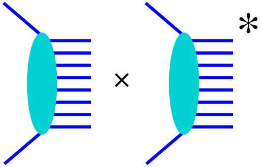
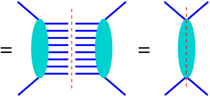
Figure 2: The expression $\sum_{X}(T_{2\rightarrow X}).$$(T_{2\rightarrow X})^{*}$which may be represented as a “cut diagram”.

So the term “cut diagram” means nothing but the square of an inelastic amplitude, summed over all final states, which is equal to twice the imaginary part of the elastic amplitude.

Before coming to nuclear collisions, we need to discuss somewhat the structure of the nucleon, which may be studied in deep inelastic scattering – so essentially the scattering of a virtual photon off a nucleon, see fig. 3.

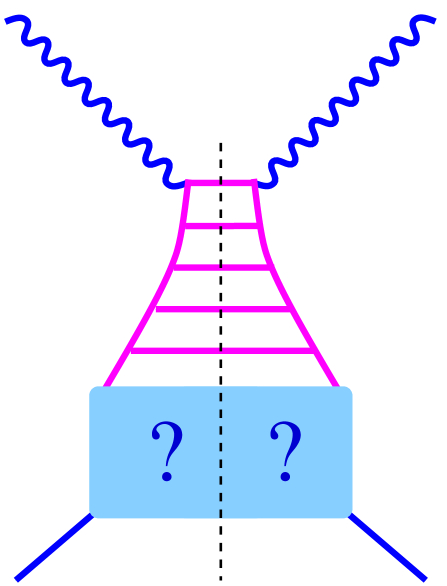
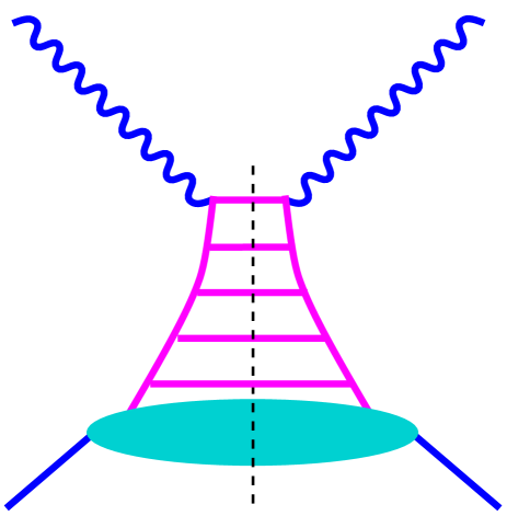
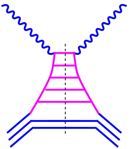
Figure 3: Deep inelastic scattering: the general diagram (left) the “sea” contribution with a soft Pomeron at the lower end (middle) and the “valence” contribution (right).

Let us assume a high virtuality photon. It is known that this photon couples to a high virtuality quark, which is emitted from a parton with a smaller virtuality, the latter on again being emitted from a parton with lower virtuality, and so on. We have a sequence of partons with lower and lower virtualities, the closer one gets to the proton. At some stage, some “soft scale” scale $Q_{0}^{2}$ must be reached, beyond which perturbative calculations are no longer valid. So we have some “unknown object” – indicated by “?” in fig. 3 – between the first parton and the nucleon. In order to proceed, one may estimate the squared mass of this “unknown object”, and one obtains doing simple kinematics the value $Q_{0}^{2}/x$, where $x$ is the momentum fraction of the first parton relative to the nucleon. Therefore, sea quarks or gluons, having typically small $x$, lead to large mass objects – which we identify with soft Pomerons, whereas valence quarks lead to small mass objects, which we simply ignore. So we have two contributions, as shown in fig. 3: a sea contribution, where the sea quark or gluon is emitted from a soft Pomeron, and a valence contribution, where the valence quark is one of the three quarks of the nucleon. The precise microscopic structure of the soft Pomeron not being known, it is parameterized in the usual way a a Regge pole.

Elementary nucleon-nucleon scattering can now be considered as a straightforward generalization of photon-nucleon scattering: one has a hard parton-parton scattering in the middle, and parton evolutions in both directions towards the nucleons. We have a hard contribution $T_{\mathrm{hard}}$ when the the first partons on both sides are valence quarks, a semi-hard contribution $T_{\mathrm{semi}}$ when at least on one side there is a sea quark (being emitted from a soft Pomeron), and finally we have a soft contribution, when there is no hard scattering at all (see fig. 4).

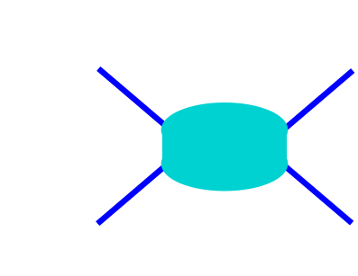
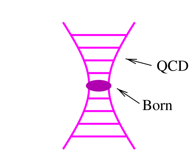
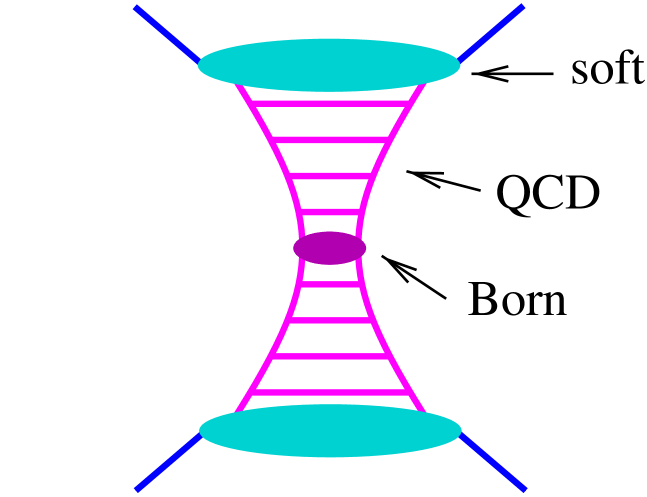
Figure 4: The soft elastic scattering amplitude $T_{\mathrm{soft}}$ (left), the hard elastic scattering amplitude $T_{\mathrm{hard}}$ (middle) and one of the three contributions to the semi-hard elastic scattering amplitude $T_{\mathrm{semi}}$ (right).

We have a smooth transition from soft to hard physics: at low energies the soft contribution dominates, at high energies the hard and semi-hard ones, at intermediate energies (that is where experiments are performed presently) all contributions are important.

Let us consider nucleus-nucleus ($AB$) scattering. In the Glauber-Gribov approach [7, 2], the nucleus-nucleus scattering amplitude is defined by the sum of contributions of diagrams, corresponding to multiple elementary scattering processes between parton constituents of projectile and target nucleons. These elementary scatterings are exactly discussed above, namely the sum of soft, semi-hard, and hard contributions: $T_{2\rightarrow 2}=T_{\mathrm{soft}}+T_{\mathrm{semi}}+T_{\mathrm{hard}}$. A corresponding relation holds for the inelastic amplitude $T_{2\rightarrow X}$. We use the above definition of a cut elementary diagram, which is graphically represented by a vertical dashed line, whereas the elastic amplitude is represented by an unbroken line:

   $=T_{2\rightarrow 2}$,           $=\sum_{X}(T_{2\rightarrow X})$$(T_{2\rightarrow X})^{*}$.

This is very handy for treating the nuclear scattering model. We define the model via the elastic scattering amplitude $T_{AB\rightarrow AB}$ which is assumed to consist of purely parallel elementary interactions between partonic constituents, as discussed above. The amplitude is therefore a sum of terms as the one shown in fig. 5.

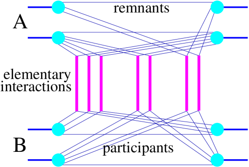
Figure 5: Elastic nucleus-nucleus scattering amplitude, being composed of purely parallel elementary interactions between partonic constituents of the nucleons (blobs).

One has to be careful about energy conservation: all the partonic constituents (lines) leaving a nucleon (blob) have to share the momentum of the nucleon. So in the explicit formula one has an integration over momentum fractions of the partons, taking care of momentum conservation. Having defined elastic scattering, inelastic scattering and particle production is practically given, if one employs a quantum mechanically self-consistent picture. Let us now consider inelastic scattering: one has of course the same parallel structure, just some of the elementary interactions may be inelastic, some elastic. The inelastic amplitude being a sum over many terms – $T_{AB\rightarrow X}=\sum_{i}T^{(i)}_{AB\rightarrow X}$ – has to be squared and summed over final states in order to get the inelastic cross section, which provides interference terms $\sum_{X}(T^{(i)}_{AB\rightarrow X})(T^{(j)}_{AB\rightarrow X})^{*}$, which can be conveniently expressed in terms of the cut and uncut elementary diagrams, as shown in fig. 6. So we are doing nothing more than following basic rules of quantum mechanics.

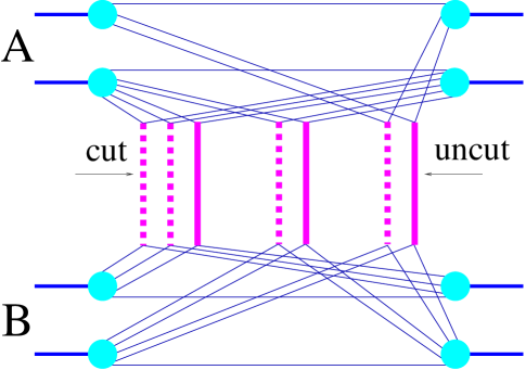
Figure 6: Typical interference term contributing to the squared inelastic amplitude.

Of course a diagram with 3 inelastic elementary interactions does not interfere with the one with 300, because the final states are different. So it makes sense to define classes $K$ of interference terms (cut diagrams) contributing to the same final state, as all diagrams with a certain number of inelastic interactions and with fixed momentum fractions of the corresponding partonic constituents. One then sums over all terms within each class $K$, and obtains for the inelastic cross section

$$\sigma_{AB}(s)=\int d^{2}b\>\sum_{K}\Omega^{(s,b)}(K)$$

where we use the symbolic notation $d^{2}b=\int d^{2}b_{0}\,\int d^{2A}b_{A}\,\rho(b_{A})\,\int d^{2B}b_{B}\,\rho(b_{B})$ which means integration over impact parameter $b_{0}$ and in addition averaging over nuclear coordinates for projectile and target. The variable $K$ is characterized by $AB$ numbers $m_{k}$ representing the number of cut elementary diagrams for each possible pair of nucleons and all the momentum fractions $x^{+}$ and $x^{-}$ of all these elementary interactions (so $K$ is a partly discrete and partly continuous variable, and $\sum$ is meant to represent $\sum\int$). This is the really new and very important feature of our approach: we keep explicitly the dependence on the longitudinal momenta, assuring energy conservation at any level of our calculation.

The calculation of $\Omega$ actually very difficult and technical, but it can be done and we refer the interested reader to the literature [3].

The quantity $\Omega^{(s,b)}(K)$ can now be interpreted as the probability to produce a configuration $K$ at given $s$ and $b$. So we have a solid basis for applying Monte Carlo techniques: one generates configurations $K$ according to the probability distribution $\Omega$ and one may then calculate mean values of observables by averaging Monte Carlo samples. The problem is that $\Omega$ represents a very high dimensional probability distribution, and it is not obvious how to deal with it. We decided to develop powerful Markov chain techniques [8] in order to avoid to introduce additional approximations.

3 New Computational Techniques

In order to generate $K$ according to the given distribution $\Omega\left(K\right)$, defined earlier, we construct a Markov chain

$$K^{\left(0\right)},K^{\left(1\right)},K^{\left(2\right)},...K^{\left(t_{\mathrm{max}}\right)}$$ (1)

such that the final configurations $K^{\left(t_{\mathrm{max}}\right)}$ are distributed according to the probability distribution $\Omega\left(K\right)$, if possible for a $t_{\mathrm{max}}$ not too large! To obtain a new configuration $K^{(t+1)}=L$ from a given configuration $K^{(t)}=K$. We use Metropolis’ Ansatz for the transition probability $p(K,L)$ as a product of a proposition matrix $w(K,L)$ and an acceptance matrix $u(K,L)$. The detailed balance condition – which assures the convergence of the chain – is automatically fulfilled if $u(K,L)$ is defined as

$$u(K,L)=\min\left(\frac{\Omega(L)}{\Omega(K)}\frac{w(L,K)}{w(K,L)},1\right).$$ (2)

We are free to choose $w(K,L)$, but of course, for practical reasons, we want to minimize the autocorrelation time, which requires a careful definition of $w$. An efficient procedure requires $u(K,L)$ to be not too small (to avoid too many rejections), so an ideal choice would be $w\left(K,L\right)=\Omega\left(L\right)$. This is of course not possible, but we choose $w(K,L)$ to be a “reasonable” approximation to $\Omega(L)$ if $K$ and $L$ are reasonably close, otherwise $w$ should be zero. So we define

$$w(K,L)=\left\{\begin{array}[]{ccc}\Omega_{0}(L)&\mathrm{if}&d(K,L)\leq 1\\ 0&\mathrm{otherwise}&\end{array}\right.,$$ (3)

where $d(K,L)$ is an integer quantity representing a distance between two configurations (the maximum number of elementary interactions being different[3]), and where $\Omega_{0}$ has a simple structure, just being a product of terms $\rho_{0}$ representing one single elementary interaction. So one proposes only new configurations being “close” to the old ones. The above definition of $w(K,L)$ may be realized by the following algorithm:

• choose randomly a particular elementary interaction (say the $\mu^{\mathrm{th}}$ interaction of the $k^{\mathrm{th}}$ nucleon-nucleon pair)

• propose a new configuration $L$, which is obtained from the old one $K$ by removing the $\mu^{\mathrm{th}}$ interaction of the $k^{\mathrm{th}}$ nucleon-nucleon pair, and replacing this by a new one according to the distribution $\rho_{0}$.

This proposal is the accepted with a probability $u(K,L)$. One should note that proposing a configuration according to some “approximation” $\Omega_{0}$ of $\Omega$ is fully compensated by the acceptance procedure, so it is an exact numerical solution of the problem, whatever be the precise definition of $\Omega_{0}$.

This procedure works extremely well. We performed many test for situations where conventional techniques work as well, and we find excellent agreement by using $66.7\,k_{\mathrm{max}}$ iterations, where $k_{\mathrm{max}}$ is an upper limit estimate of the number of nucleon-nucleon interactions. The Markov-chain method is perfect for our purposes, because we have fast convergence due to the fact that $\Omega_{0}$ is not too different from $\Omega$, on the other hand one cannot use just $\Omega_{0}$ to obtain an approximate solution, because here we introduce an substantial error, which reaches for example already on the nucleon-nucleon level about 100 %.

4 Summary

We provide a new formulation of the multiple scattering mechanism in nucleus-nucleus scattering, where the basic guideline is theoretical consistency. We avoid in this way many of the problems encountered in present day models. We also introduce the necessary numerical techniques to apply the formalism in order to perform practical calculations.

This work has been funded in part by the IN2P3/CNRS (PICS 580) and the Russian Foundation of Basic Researches (RFBR-98-02-22024).

References

- [1] V. N. Gribov, Sov. Phys. JETP 26, 414 (1968).
- [2] V. N. Gribov, Sov. Phys. JETP 29, 483 (1969).
- [3] H. J. Drescher, M. Hladik, S. Ostapchenko, T. Pierog, and K. Werner, (2000), hep-ph/0007198, to be published in Physics Reports.
- [4] M. Braun, Yad. Fiz. (Rus) 52, 257 (1990).
- [5] V. A. Abramovskii and G. G. Leptoukh, Sov.J.Nucl.Phys. 55, 903 (1992).
- [6] T. Sjostrand and M. van Zijl, Phys. Rev. D36, 2019 (1987).
- [7] R. J. Glauber, in Lectures on theoretical physics (N.Y.: Inter-science Publishers, 1959).
- [8] M. Hladik, Nouvelle approche pour la diffusion multiple dans les interactions noyau-noyau aux énergies ultra-relativistes, PhD thesis, Université de Nantes, 1998.