Low $x$ double $ln^{2}(1/x)$ resummation effects at the sum rules for nucleon structure function $g_{1}$

Abstract

We have estimated the contributions to the moments of polarized nucleon structure function $g_{1}(x,Q^{2})$ coming from the region of the very low x ($10^{-5}<x$). Our approach uses the nucleon structure function extrapolated to the region of low $x$ by the means of the double $ln^{2}(1/x)$ resummation. The $Q^{2}$ evolution of $g_{1}$ was described by the unified evolution equations incorporating both the leading order Altarelli-Parisi evolution at large and moderate $x$, and the double $ln^{2}(1/x)$ resummation at small $x$. The moments were obtained by integrating out the extrapolated nucleon structure function in the region $10^{-5}<x<1$.

Abbreviations footnote:

AP-Altarelli-Parisi,
LO-leading-order,
NLO-next-to-leading order,
QCD-quantum chromodynamics,

1 Introduction

The sum rules which are expected to be satisfied by the spin-dependent structure function $g_{1}$ of the nucleon play a very important role in the theory of the spin-dependent deep inelastic lepton scattering [1]. The sum rules involve (first) moments of the spin-dependent structure functions, and the moment integrals require knowledge of those structure functions in the entire region $0<x<1$ where, as usual, $x$ denotes the Bjorken variable. Presently available experiments cover only the region of large and moderately small values of $x$ ($x>5\cdot 10^{-3}$) for reasonably large values of the photon virtuality $Q^{2}$ ($Q^{2}>5GeV^{2}$). Hence, a reliable theoretical estimate of the contributions to the moment integrals coming from the unmeasured small $x$ region is important for the analysis of the sum rules.

In this paper we propose an extrapolation of the spin-dependent parton distributions and of the polarized nucleon structure functions into the low $x$ region. The extrapolation is based on the double $ln^{2}(1/x)$ resummation [2, 3]. After integrating out the parton distributions or structure functions, one obtains the low $x$ contribution to the corresponding moments. The integration interval extends from $x\sim 10^{-5}$ to $x=1$. It is assumed here that the small $x$ behaviour of $g_{1}$ is controlled by the double $ln^{2}(1/x)$ resummation. The full analysis of the double $ln^{2}(1/x)$ resummation effects was performed in detail in Ref. [2]. The dominant contribution generating the double logarithmic terms is given by the ladder diagrams with the quark (antiquark) and gluon exchanges along the ladder. The very transparent way of resumming these terms is provided by the formalism of the unintegrated (spin-dependent) parton distributions which satisfy the corresponding integral equations. In [4] we extended this formalism so as to include the non-ladder bremsstrahlung terms by adding the suitable higher order corrections to the kernels of the corresponding integral equations. We also incorporated the complete leading-order (LO) Altarelli-Parisi (AP) evolution within this scheme, thus obtaining the unified system of equations able to analyse simultaneously the parton distributions in the large and small $x$ regions. In particular, this formalism allows us to extrapolate dynamically the spin-dependent structure functions from the region of large and moderately small values of $x$, where they are constrained by the presently available data to the very small $x$ domain which can possibly be probed at the polarized HERA [5].

This paper is organized as follows. In section 2 we recall briefly Bjorken and Ellis-Jaffe sum rules for nucleon structure functions. In section 3 the unified evolution equations for $g_{1}(x,Q^{2})\,\,\,\,$[4] which embody both complete LO AP evolution at large values of $x$ and the full (ladder and non-ladder) double $ln^{2}(1/x)$ resummation at small $x$ are discussed in the context of the partonic moment conservation. It is shown that in the non-singlet sector the first moments of both baryonic isovector $g_{1}^{NS}(x,Q^{2})$ and baryonic octet $g_{1}^{(8)}(x,Q^{2})$ are conserved, i.e. they are independent of $Q^{2}$. It is also shown that there is no first moment conservation in the singlet sector. It should be recalled that the first moments of the non-singlet and octet structure functions acquire their $Q^{2}$ dependence only as the result of the next-to-leading order (NLO) quantum chromodynamics (QCD) effects. Our formalism extends the LO AP formalism by including the small $x$ resummation, yet it does not affect the conservation of the first moments of structure functions.

In Section 4 our predictions for Bjorken and Ellis-Jaffe sum rules obtained after numerical integration of the respective nucleon components in the region extending from very low $x$ ($10^{-5}<x$) are presented. First moments of nucleon structure functions are calculated and compared with experimental data [6, 7, 8, 9, 10, 11, 12, 13, 14]. In order to estimate the impact of the low $x$ region on the sum rule integrals and moments, partial contributions from very low $x$ region $10^{-5}<x<10^{-3}$ are calculated explicitly. In our approach we use a simple semi-phenomenological parametrization of the non-perturbative part of the spin-dependent parton distributions.

In Section 5 the summary of our results is given.

2 Sum rules for $g_{1}(x,Q^{2})$

The sum rules for polarized nucleon structure functions are derived from the space-time representation of scattering amplitudes $T_{ik}^{a}(x)$ in terms of current commutators [15, 16] :

$$Im\,T_{ik}(x)=\frac{1}{4}\,\langle p,s\mid\,\left[j_{i},j_{k}\right]_{antisym.\ }\,\mid p,s\rangle.$$ (1)

In the light cone limit $x^{2}\rightarrow 0$, $x_{0}\rightarrow 0$, which corresponds to parton model kinematics, they reduce to:

$$\lim_{x_{0}\rightarrow 0}\,Im\,T_{ik}(x)=-\epsilon_{ikl}\langle p,s\mid\frac{1}{3}\left[j_{5l}^{3}(0)+\sqrt{\frac{1}{3}}j_{5l}^{8}(0)\right]+\frac{2}{9}\,j_{5l}^{0}(0)\mid p,s\rangle.$$ (2)

The isospin symmetry determines the proton matrix element of the isovector current $j_{5l}^{3}(0)$, and results in the Bjorken sum rule for the non-singlet component of the nucleon structure functions $g_{1}^{p,n}(x,Q^{2})$ which in LO approximation reads :

$$\int_{0}^{1}\,g_{1}^{BJ}(x,Q^{2})=g_{A}/6,$$ (3)

where $g_{1}^{BJ}(x,Q^{2})\equiv g_{1}^{p}(x,Q^{2})-g_{1}^{n}(x,Q^{2})$, $g_{1}^{p}$, $g_{1}^{n}$ are proton and neutron structure functions respectively, and $g_{A}\approx 1.257$ is the neutron $\beta$-decay axial coupling constant. It should be stated clearly that the Bjorken sum rule acquires also corrections beyond the LO approximation. Since the formalism of the unified evolution equations we use henceforth includes only the LO AP evolution, we neglect the NLO correction terms both for the Bjorken and the Ellis-Jaffe sum rule.

The Ellis-Jaffe sum rule for baryonic octet follows, if $SU(3)$ flavour symmetry for octet $\beta$-decays is assumed :

$$\int_{0}^{1}\,g_{1}^{8}(x,Q^{2})=(3F-D)/24,$$ (4)

where :

$$g_{1}^{8}(x,Q^{2})=(\Delta u+\Delta d-2\Delta s)/24,$$ (5)

and $F$, $D$ are octet $\beta$-decay axial coupling constants [15] fulfilling the relation $(3F-D)/24\approx 0.0241$. Distributions $\Delta u$, $\Delta d$, $\Delta s$ denote quark components of the polarized nucleon.

3 Moments of $g_{1}(x,Q^{2})\,\,\,\,$and double $ln^{2}(1/x)$ resummation

Low $x$ behaviour of polarized nucleon structure function is influenced by double logarithmic $ln^{2}(1/x)$ contributions, i. e.  by those terms of the perturbative expansion, which correspond to the powers of $ln^{2}(1/x)$ at each order of the expansion [17, 18]. In what follows we will apply the double $ln^{2}(1/x)$ resummation scheme based on the unintegrated parton distributions [19, 2, 20]. Conventional integrated spin-dependent parton distributions $\Delta p_{l}(x,Q^{2})$ ($p=q,g$) are related to the unintegrated parton distributions $f_{l}(x^{\prime},k^{2})$ in the following way  :

$$\Delta p_{l}(x,Q^{2})=\Delta p_{l}^{(0)}(x)+\int_{k_{0}^{2}}^{W^{2}}{dk^{2}\over k^{2}}\,f_{l}(x^{\prime}=x(1+{k^{2}\over Q^{2}}),k^{2}),$$ (6)

where $\Delta p_{l}^{(0)}(x)$ is the nonperturbative part of the distribution, $k^{2}$ denotes the transverse momentum squared of the probed parton, $W^{2}$ is the total energy in the center of mass $W^{2}=Q^{2}\,(\frac{1}{x}-1)$, and index $l$ specifies the parton flavour. The parameter $k_{0}^{2}$ is the infrared cut-off, which will be set equal to 1 GeV². The nonperturbative part $\Delta p_{l}^{(0)}(x)$ can be viewed upon as originating from the integration over non-perturbative region $k^{2}<k_{0}^{2}$, i. e.

$$\Delta p_{l}^{(0)}(x)=\int_{0}^{k_{0}^{2}}{dk^{2}\over k^{2}}f_{l}(x,k^{2}).$$ (7)

The nucleon structure function $g_{1}(x,Q^{2})$ is related in a standard way to the (integrated) parton distributions describing the parton content of the polarized nucleon :

$$g_{1}^{p}(x,Q^{2}) = \frac{\langle e^{2}\rangle}{2}\,[g_{1}^{S}(x,Q^{2})+g_{1}^{NS,p}(x,Q^{2})],$$ (8)

$$g_{1}^{n}(x,Q^{2}) = \frac{\langle e^{2}\rangle}{2}\,[g_{1}^{S}(x,Q^{2})+g_{1}^{NS,n}(x,Q^{2})],$$ (9)

where $N_{f}$ denotes the number of active flavours ($N_{f}=3$) and $\displaystyle\langle e^{m}\rangle={1\over N_{f}}\sum_{l=1}^{N_{f}}(e_{l})^{m}$. For convenience we have introduced in (8), (9) the non-singlet and singlet combinations of the spin-dependent quark and antiquark distributions defined for proton and neutron as:

$$g_{1}^{NS,p(n)}(x,Q^{2})=\sum_{l=1}^{N_{f}}\left({e_{l}^{2}\over\langle e^{2}\rangle}-1\right)(\Delta q^{p(n)}_{l}(x,Q^{2})+\Delta\overline{q}^{p(n)}_{l}(x,Q^{2})),$$ (10)

$$g_{1}^{S}(x,Q^{2})=\sum_{l=1}^{N_{f}}(\Delta q^{\gamma}_{l}(x,Q^{2})+\Delta\overline{q}^{\gamma}_{l}(x,Q^{2})).$$ (11)

In order to consider the Ellis-Jaffe sum rule we shall also analize the baryon octet structure function $g^{8}(x,Q^{2})$, defined by equation (5).

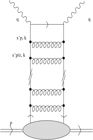
Figure 1: Ladder diagram generating the double logarithmic terms in the non-singlet component of the spin structure function.

Figure 2: The moment $I_{1}^{p}$ of proton structure function $g_{1}^{p}(x,Q^{2})$ plotted as a function of $Q^{2}$. Solid line denotes results obtained from the unified evolution including the full double logarithmic resummation $ln^{2}(1/x)$, dashed line shows pure AP evolution, dotted line corresponds to the non-perturbative input (overlaps with AP results). Experimental data are denoted: E143 [7] with vertical bars, SMC [8] with stars, EMC [9] with white squares.

Figure 3: The moment $I_{1}^{n}$ of neutron structure function $g_{1}^{n}(x,Q^{2})$ plotted as a function of $Q^{2}$. Solid line denotes results obtained from the unified evolution including the full double logarithmic resummation $ln^{2}(1/x)$, dashed line shows pure AP evolution, dotted line corresponds to the non-perturbative input (overlaps with AP results). Experimental data are denoted: E143 [10] with vertical bars, SMC [11] with crosses, E154 [9] with stars, E142 [13] with white squares, HERMES [14] with black squares.

Figure 4: The ratio $R^{BJ}(Q^{2})$ for Bjorken sum rule integral plotted as a function of $Q^{2}$. Solid line denotes results obtained from the unified evolution including the full double logarithmic resummation $ln^{2}(1/x)$, dashed line shows pure AP evolution, dotted line corresponds to the non-perturbative input.

Figure 5: The ratio $R^{8}(Q^{2})$ for Ellis-Jaffe sum rule integral plotted as a function of $Q^{2}$. Solid line denotes results obtained from the unified evolution including the full double logarithmic resummation $ln^{2}(1/x)$, dashed line shows pure AP evolution, dotted line corresponds to the non-perturbative input.

Figure 6: The ratio $R^{p}(Q^{2})$ for the first moment of proton structure function plotted as a function of $Q^{2}$. Solid line denotes results obtained from the unified evolution including the full double logarithmic resummation $ln^{2}(1/x)$, dashed line shows pure AP evolution, dotted line corresponds to the non-perturbative input.

Figure 7: The ratio $R^{n}(Q^{2})$ for the first moment of neutron structure function plotted as a function of $Q^{2}$. Solid line denotes results obtained from the unified evolution including the full double logarithmic resummation $ln^{2}(1/x)$, dashed line shows pure AP evolution, dotted line corresponds to the non-perturbative input.

The full contribution to the double $ln^{2}(1/x)$ resummation comes from the ladder diagrams with quark and gluon exchanges along the ladder (cf. Fig. 1) and the non-ladder bremsstrahlung diagrams [21, 22]. The latter ones are obtained from the ladder diagrams by adding to them soft bremsstrahlung gluons or soft quarks [17, 18, 21, 22]. They generate the infrared corrections to the ladder contribution.

The relevant region of phase space generating the double $ln^{2}(1/x)$ resummation from ladder diagrams corresponds to ordered $k_{n}^{2}/x_{n}$, where $k_{n}^{2}$ and $x_{n}$ denote respectively the transverse momenta squared and longitudinal momentum fractions of the proton, carried by partons exchanged along the ladder [23, 24]. It is in contrast to the LO AP evolution alone, which corresponds to ordered transverse momenta.

The structure of the corresponding integral equations describing unintegrated distributions $f_{NS}(x{{}^{\prime}},k^{2}),f_{S}(x{{}^{\prime}},k^{2})$ and $f_{g}(x{{}^{\prime}},k^{2})$ for ladder diagram contribution read [2]:

$$f_{NS}(x^{\prime},k^{2})=f^{(0)}_{NS}(x^{\prime},k^{2})+{\alpha_{S}\over 2\pi}\Delta P_{qq}(0)\int_{x^{\prime}}^{1}{dz\over z}\int_{k_{0}^{2}}^{k^{2}/z}{dk^{\prime 2}\over k^{\prime 2}}f_{NS}\left({x^{\prime}\over z},k^{\prime 2}\right),$$ (12)

$$f_{S}(x^{\prime},k^{2})=f^{(0)}_{S}(x^{\prime},k^{2})+{\alpha_{S}\over 2\pi}\int_{x^{\prime}}^{1}{dz\over z}\int_{k_{0}^{2}}^{k^{2}/z}{dk^{\prime 2}\over k^{\prime 2}}\left[\Delta P_{qq}(0)f_{S}\left({x^{\prime}\over z},k^{\prime 2}\right)+\Delta P_{qg}(0)f_{g}\left({x^{\prime}\over z},k^{\prime 2}\right)\right],$$

$$f_{g}(x^{\prime},k^{2})=f^{(0)}_{g}(x^{\prime},k^{2})+{\alpha_{S}\over 2\pi}\int_{x^{\prime}}^{1}{dz\over z}\int_{k_{0}^{2}}^{k^{2}/z}{dk^{\prime 2}\over k^{\prime 2}}\left[\Delta P_{gq}(0)f_{S}\left({x^{\prime}\over z},k^{\prime 2}\right)+\Delta P_{gg}(0)f_{g}\left({x^{\prime}\over z},k^{\prime 2}\right)\right]$$

(13)

with splitting functions $\Delta P_{ij}(0)\equiv\Delta P_{ij}(z=0)$ equal to :

$${\bf\Delta P(0)}\equiv\left(\begin{array}[]{cc}\Delta P_{qq}(0)&\Delta P_{qg}(0)\\ \Delta P_{gq}(0)&\Delta P_{gg}(0)\\ \end{array}\right)=\left(\begin{array}[]{cc}{{N_{C}^{2}-1\over 2N_{C}}}&-N_{F}\\ {{N_{C}^{2}-1\over N_{C}}}&4N_{C}\\ \end{array}\right),$$ (18)

where $\alpha_{S}$ denotes the QCD coupling, which at the moment is treated as a fixed parameter. The variables $k^{2}$($k^{\prime 2}$) denote the transverse momenta squared of the quarks (gluons), exchanged along the ladder. For the parton distributions in a hadron the inhomogeneous driving terms $f^{(0)}_{l}(x^{\prime},k^{2})$ are entirely determined by the non-perturbative parts $\Delta p_{i}^{(0)}(x^{\prime})$ of the spin-dependent parton distributions.

Besides the ladder diagrams contributions, the double logarithmic resummation does also acquire corrections from the non-ladder bremsstrahlung contributions. It has been shown in Ref. [2] that these contributions can be included by adding the higher order terms to the kernels of integral equations (12), (13). These terms can be obtained from the matrix: $\displaystyle\Biggl{[}{\tilde{\bf F}_{8}}/\omega^{2}\Biggr{]}(z)\bf G_{0}$, where $\displaystyle\Biggl{[}\frac{\tilde{\bf F}_{8}}{\omega^{2}}\Biggr{]}(z)$ denote the inverse Mellin transform of the octet partial wave matrix (divided by $\omega^{2}$ ), and the matrix $\bf G_{0}$ reads:

$${\bf G}_{0} = \left(\begin{array}[]{cc}{N_{c}^{2}-1\over 2N_{c}}&0\\ 0&N_{c}\\ \end{array}\right).$$ (21)

Following Ref. [2], we shall use the Born approximation for the octet matrix :

$$\Biggl{[}\frac{\tilde{\bf F}_{8}^{Born}}{\omega^{2}}\Biggr{]}(z)=4\pi^{2}\overline{\alpha}_{S}{\bf M}_{8}ln^{2}(z),$$ (22)

where $\bf M_{8}$ is the splitting functions matrix in colour octet t-channel :

$${\bf M}_{8} = \left(\begin{array}[]{cc}-{1\over 2N_{c}}&-{N_{F}\over 2}\\ N_{c}&2N_{c}\\ \end{array}\right).$$ (25)

In the region of large values of $x$ the integral equations (12), (13) describing pure double logarithmic resummation $\ln^{2}(1/x)$, even completed by including non-ladder contributions, are inaccurate. In this region one should use the conventional AP equations [25, 26, 27] with the complete splitting functions $\Delta P_{ij}(z)$ and not restrict oneself to the effect generated by their $z\rightarrow 0$ part. Following Refs. [19, 2], we do therefore extend equations (12), (13), and add to their right-hand-side(s) the contributions coming from the remaining parts of the splitting functions $\Delta P_{ij}(z)$. We also allow coupling $\alpha_{S}$ to run, setting $k^{2}$ as the relevant scale. In this way we obtain unified system of equations, which contain both the complete leading order AP evolution and the double logarithmic $ln^{2}(1/x)$ effects at low $x$. These equations are listed in Appendix A.

3.1 Conservation of moments

In order to get information about the moments of spin structure functions, we will follow the technique proposed in [19]. First we integrate the integrated parton distributions (6) over $x$ :

$$\int_{0}^{1}\,dx\,\Delta p_{l}(x,Q^{2})=\int_{0}^{1}\,dx\,\Delta p_{l}^{(0)}(x)+\int_{k_{0}^{2}}^{\infty}{dk^{2}\over{k^{2}(1+\frac{k^{2}}{Q^{2}})}}\,\int_{0}^{1}\,dx\,f_{l}(x,k^{2}).$$ (26)

Let us denote ${\overline{\Delta}p_{l}(Q^{2})}\,\equiv\,\int_{0}^{1}\,dx\,\Delta p_{l}(x,Q^{2})$, and respectively ${\overline{f}_{l}(k^{2})}\,\equiv\,\int_{0}^{1}\,dx\,f_{l}(x,k^{2})$. Since structure functions $g_{1}^{NS\,(S)}(x,Q^{2})$ (10), (11) are linear combinations of (6), their moments may be obtained as :

$${\overline{g}_{1}^{NS}(Q^{2})} = {\overline{g}_{1}^{NS,(0)}}+\int_{k_{0}^{2}}^{\infty}{dk^{2}\over{k^{2}(1+\frac{k^{2}}{Q^{2}})}}{\overline{f}_{NS}(k^{2})},$$ (27)

$${\overline{g}_{1}^{S}(Q^{2})} = {\overline{g}_{1}^{S,(0)}}+\int_{k_{0}^{2}}^{\infty}{dk^{2}\over{k^{2}(1+\frac{k^{2}}{Q^{2}})}}{\overline{f}_{S}(k^{2})},$$ (28)

where ($i=NS,S$) :

$${\overline{g}_{1}^{i}} = \int_{0}^{1}\,dx\,g_{1}^{i}(x),$$ (29)

$${\overline{g}_{1}^{i,(0)}} = \int_{0}^{1}\,dx\,g_{1}^{i,(0)}(x).$$ (30)

Furthermore, for non-singlet sector it was proven [19] (see Appendix B) that the moments of $f^{(0)}_{NS}(x^{\prime},k^{2})$ (42) vanish independently of the input $g_{1}^{NS(0)}(x)$ :

$${\overline{f}_{NS}^{(0)}(k^{2})}=0.$$ (31)

Therefore the unified equation for moments ${\overline{f}_{NS}(k^{2})}$, obtained from equation (Appendix A) after integration over $x$, reduces to the integral equation with inhomogeneous term equal to $0$. Its solution then reads :

$${\overline{f}_{NS}(k^{2})}=0.$$ (32)

For the singlet sector the situation gets more complicated. Although the quark singlet moment :

$${\overline{f}_{S}^{(0)}(k^{2})}=0$$ (33)

vanishes again (see Appendix C), the moment of the input gluon distribution ${\overline{f}_{g}^{(0)}(k^{2})}$ takes a non-zero value which reads :

$${\overline{f}_{g}^{(0)}(k^{2})}=\frac{\alpha_{S}(k^{2})}{2\pi}\,\left[2\,{\overline{g}_{1}^{S,(0)}}+({11\over 2}-{N_{F}\over 3}){\overline{\Delta}p_{g}^{(0)}}\right].$$ (34)

Hence, the unified equations for quark singlet and gluon moments, obtained from coupled equations (Appendix A), (Appendix A) get a non-zero inhomogeneous term in the gluon sector, and the moment ${\overline{f}_{S}(k^{2})}$ is non-vanishing as well.

The properties of partonic moments resulting from the unified equations (Appendix A), (Appendix A), (Appendix A) after transforming them into the moment space have clear implications for Bjorken and Ellis-Jaffe sum rules. Both Bjorken and Ellis-Jaffe sum rules (3), (4) concern evolution in the non-singlet sector. Hence, if one assumes input distributions $g_{1}^{BJ,(0)}$ and $g_{1}^{8,(0)}$ fulfilling the requirements (3), (4), it follows from relations (27), (32) that :

$${\overline{g}_{1}^{BJ}(Q^{2})} = {\overline{g}_{1}^{BJ,(0)}}=const,$$ (35)

$${\overline{g}_{1}^{8}(Q^{2})} = {\overline{g}_{1}^{8,(0)}}=const$$ (36)

are conserved throughout whole $Q^{2}$ evolution.

The non-vanishing unintegrated gluon input (34) implies that there is no explicit conservation of ${\overline{g}_{1}^{S}(Q^{2})}$ ( and ${\bar{\Delta}g(Q^{2})}$ ) during $Q^{2}$ evolution. However, the conservation may be achieved implicitly by imposing the negative input gluon distribution ${\overline{\Delta}p_{g}^{(0)}}$ to fulfill the requirement :

$$2\,{\overline{g}_{1}^{S,(0)}}+({11\over 2}-{N_{F}\over 3}){\overline{\Delta}p_{g}^{(0)}}=0.$$ (37)

This is not a physical case but this shows that the moments are very sensitive to the gluon input which, in fact, has not an established phenomenological parametrization because of the lack of experimental data. Therefore, there is still possible to influence the $Q^{2}$ evolution of ${\overline{g}_{1}^{S,(0)}}$ and henceforth, the evolution of $\Gamma^{1,p,n}(Q^{2})$ by manipulating the input gluon distribution.

4 Numerical results for sum rules

We solved the unified equations (Appendix A), (Appendix A), (Appendix A), assuming the following simple parametrization of the input distributions:

$$\Delta p_{i}^{(0)}(x)=N_{i}(1-x)^{\eta_{i}}$$ (38)

with $\eta_{u_{v}}=\eta_{d_{v}}=3,$ $\eta_{\overline{u}}=\eta_{\overline{s}}=7$ and $\eta_{g}=5$. The normalisation constants $N_{i}$ were determined by imposing the Bjorken sum rule for $\Delta u_{v}^{(0)}-\Delta d_{v}^{(0)}$ and requiring that the first moments of all other distributions are the same as those determined from the recent QCD analysis [28]. All distributions $\Delta p_{i}^{(0)}(x)$ behave as $x^{0}$ in the limit $x\rightarrow 0$ that corresponds to the implicit assumption that the Regge poles which should control the small $x$ behaviour of $g_{1}^{(0)}$ have their intercept equal to $0$.

It was checked that the parametrization (38) combined with equations (6), (10), (11), (Appendix A), (Appendix A), (Appendix A) gives reasonable description of the recent SMC data on $g_{1}^{BJ}(x,Q^{2})$ and on $g_{1}^{p}(x,Q^{2})$ [11]. After integrating out the respective parton distributions, we found that the moments ${\overline{g}_{1}^{BJ}(Q^{2})}$ and ${\overline{g}_{1}^{8}(Q^{2})}$ are conserved during $Q^{2}$ evolution with a good accuracy (not shown). The Bjorken sum rule is conserved explicitly, due to the choice of the input (${\overline{g}_{1}^{BJ,(0)}(Q^{2})}\approx 0.2095$). For the ${\overline{g}_{1}^{8}(Q^{2})}$ moment, the input was chosen to give ${\overline{g}_{1}^{8,(0)}(Q^{2})}\approx 0.016$, which was implicitly in disagreement with hyperon $\beta$-decay data (5).

We also investigated the $Q^{2}$ evolution of the first moments of $g_{1}^{p,n}(x,Q^{2})$ and compared them with experimental data (see Figs. 2, 3). First moments of $g_{1}^{p}(x,Q^{2})$ agree well with the available experimental data both for moments obtained after performing LO AP evolution of non-perturbative input and for moments obtained after solving the unified evolution equation (cf. Fig. 2). On the contrary, our predictions for the first moments of polarized neutron structure function $g_{1}^{n}(x,Q^{2})$ obtained from both the unified and the AP evolution are below the experimental data (cf. Fig. 3). The discrepancy may be due to the fact that we consider only the LO AP evolution of the partonic moments. Also the Bjorken sum rule is considered at LO accuracy. Since the AP evolution dominates in the region of moderate and large $x$, applying it with the leading order (parton model) accuracy may be not sufficient to reproduce the experimental data.

Moreover, we estimated the magnitude of contribution from the very low $x$ region ($10^{-5}<x<10^{-3}$) to the moments of polarized nucleon structure function. It was achieved by comparing the partial contributions with the total moments obtained after integrating $g_{1}^{p,n}$ over $x$ extending from $10^{-5}$ to $1$. The calculated ratios, $\displaystyle R^{i}\equiv{\overline{g}_{1}^{i,L}(Q^{2})}/{\overline{g}_{1}^{i}(Q^{2})}$ ($i=BJ,8,p,n$), where $\displaystyle{\overline{g}_{1}^{i,L}(Q^{2})}\,\equiv\,\int_{10^{-5}}^{10^{-3}}\,dx\,g_{1}^{i}(x,Q^{2})$, are plotted in Figs. 4, 5, 6, 7. For Bjorken integral (BJ) (3) the maximal $\mid R^{BJ}\mid$ is $\sim 0.02$, and for baryonic octet ($8$), $\mid R^{8}\mid\sim 0.01$. For proton (p) the maximal contribution of low $x$ region to the first moment of the proton structure function is $\mid R^{p}\mid\sim 0.02$, and for neutron (n), $\mid R^{n}\mid\sim 0.08$.

5 Summary

To sum up, we have estimated the contributions to the moments of polarized nucleon structure function $g_{1}(x,Q^{2})$ coming from the region of the very low x ($10^{-5}<x$). Our approach used the nucleon structure function extrapolated to the region of low $x$ by the means of the double $ln^{2}(1/x)$ resummation which dominates in this region. The $Q^{2}$ evolution of $g_{1}$ was described by the unified evolution equations, which incorporated both the LO AP evolution manifesting at large and moderate $x$, and double $ln^{2}(1/x)$ resummation dominating at small $x$. These moments were obtained by integrating out the extrapolated nucleon structure function in the region $10^{-5}<x<1$.

Moments of proton structure function estimated for $2<Q^{2}<15$ GeV² were found in agreement with experimental data. The explicitly evaluated contribution of low $x$ region obtained via integrating out the $g_{1}(x,Q^{2})$ in the region of very low $x$ ($10^{-5}<x<10^{-3}$) was found to constitute about 2% of the total proton moment for $2<Q^{2}<15$ GeV².

Moments of neutron structure function estimated for $2<Q^{2}<15$ GeV² were found to lie below the experimental data. This may be due to the fact that the unified evolution equations contain only leading order AP kernels. The contribution of the very low $x$ region ($10^{-5}<x<10^{-3}$) was found to constitute around 8% of the total neutron moment for $2<Q^{2}<15$ GeV².

Contributions from very low $x$ region to Bjorken and Ellis-Jaffe sum rules were of the order $1$ % and $2$ % respectively.

This implies that the contribution of low $x$ region enters the moments of polarized nucleon structure function at the level of 10 % at most. The contribution increases with increasing $Q^{2}$. We expect that the improvements of the model needed to describe accurately the neutron data will possibly affect only the normalization of the corresponding integrals, and they will not change significantly the estimate of the relative contributions coming from the low x region.

Appendix A

The corresponding system of equations reads :

$$f_{NS}(x^{\prime},k^{2})=f^{(0)}_{NS}(x^{\prime},k^{2}) + {\alpha_{S}(k^{2})\over 2\pi}{4\over 3}\int_{x^{\prime}}^{1}{dz\over z}\int_{k_{0}^{2}}^{k^{2}/z}{dk^{\prime 2}\over k^{\prime 2}}f_{NS}\left({x^{\prime}\over z},k^{\prime 2}\right)$$

$$\hskip 38.74985pt{\bf(\hskip 11.62495ptLadder\hskip 11.62495pt)}$$

$$+ {\alpha_{S}(k^{2})\over 2\pi}\int_{k_{0}^{2}}^{k^{2}}{dk^{\prime 2}\over k^{\prime 2}}{4\over 3}\int_{x^{\prime}}^{1}{dz\over z}{(z+z^{2})f_{NS}({x^{\prime}\over z},k^{\prime 2})-2zf_{NS}(x^{\prime},k^{\prime 2})\over 1-z}$$

$$+ {\alpha_{S}(k^{2})\over 2\pi}\int_{k_{0}^{2}}^{k^{2}}{dk^{\prime 2}\over k^{\prime 2}}\left[2+{8\over 3}ln(1-x^{\prime})\right]f_{NS}(x^{\prime},k^{\prime 2})$$

$$\hskip 38.74985pt{\bf(\hskip 11.62495ptAltarelli-Parisi\hskip 15.49994pt)}$$

$$- {\alpha_{S}(k^{2})\over 2\pi}\int_{x^{\prime}}^{1}{dz\over z}\Biggl{(}\Biggl{[}\frac{\tilde{\bf F}_{8}}{\omega^{2}}\Biggr{]}(z)\frac{{\bf G}_{0}}{2\pi^{2}}\Biggr{)}_{qq}\int_{k_{0}^{2}}^{k^{2}}{dk^{\prime 2}\over k^{\prime 2}}f_{NS}\left({x^{\prime}\over z},k^{\prime 2}\right)$$

$$- {\alpha_{S}(k^{2})\over 2\pi}\int_{x^{\prime}}^{1}{dz\over z}\int_{k^{2}}^{k^{2}/z}{dk^{\prime 2}\over k^{\prime 2}}\Biggl{(}\Biggl{[}\frac{\tilde{\bf F}_{8}}{\omega^{2}}\Biggr{]}\Biggl{(}\frac{k^{\prime 2}}{k^{2}}z\Biggr{)}\frac{{\bf G}_{0}}{2\pi^{2}}\Biggr{)}_{qq}f_{NS}\left({x^{\prime}\over z},k^{\prime 2}\right),$$

$$\hskip 38.74985pt{\bf(Non-ladder)}$$

$$f_{S}(x^{\prime},k^{2})=f^{(0)}_{S}(x^{\prime},k^{2}) + {\alpha_{S}(k^{2})\over 2\pi}\int_{x^{\prime}}^{1}{dz\over z}\int_{k_{0}^{2}}^{k^{2}/z}{dk^{\prime 2}\over k^{\prime 2}}{4\over 3}f_{S}\left({x^{\prime}\over z},k^{\prime 2}\right)$$

$$- {\alpha_{S}(k^{2})\over 2\pi}\int_{x^{\prime}}^{1}{dz\over z}\int_{k_{0}^{2}}^{k^{2}/z}N_{F}{dk^{\prime 2}\over k^{\prime 2}}f_{g}\left({x^{\prime}\over z},k^{\prime 2}\right)$$

$$\hskip 38.74985pt{\bf(\hskip 11.62495ptLadder\hskip 11.62495pt)}$$

$$+ {\alpha_{S}(k^{2})\over 2\pi}\int_{k_{0}^{2}}^{k^{2}}{dk^{\prime 2}\over k^{\prime 2}}{4\over 3}\int_{x^{\prime}}^{1}{dz\over z}{(z+z^{2})f_{S}({x^{\prime}\over z},k^{\prime 2})-2zf_{S}(x^{\prime},k^{\prime 2})\over 1-z}$$

$$+ {\alpha_{S}(k^{2})\over 2\pi}\int_{k_{0}^{2}}^{k^{2}}{dk^{\prime 2}\over k^{\prime 2}}\left[2+{8\over 3}ln(1-x^{\prime})\right]f_{S}(x^{\prime},k^{\prime 2})$$

$$+ {\alpha_{S}(k^{2})\over 2\pi}\int_{k_{0}^{2}}^{k^{2}}{dk^{\prime 2}\over k^{\prime 2}}\int_{x^{\prime}}^{1}{dz\over z}2zN_{F}f_{g}({x^{\prime}\over z},k^{\prime 2})$$

$$\hskip 38.74985pt{\bf(\hskip 11.62495ptAltarelli-Parisi\hskip 15.49994pt)}$$

$$- {\alpha_{S}(k^{2})\over 2\pi}\int_{x^{\prime}}^{1}{dz\over z}\Biggl{(}\Biggl{[}\frac{\tilde{\bf F}_{8}}{\omega^{2}}\Biggr{]}(z)\frac{{\bf G}_{0}}{2\pi^{2}}\Biggr{)}_{qq}\int_{k_{0}^{2}}^{k^{2}}{dk^{\prime 2}\over k^{\prime 2}}f_{S}\left({x^{\prime}\over z},k^{\prime 2}\right)$$

$$- {\alpha_{S}(k^{2})\over 2\pi}\int_{x^{\prime}}^{1}{dz\over z}\int_{k^{2}}^{k^{2}/z}{dk^{\prime 2}\over k^{\prime 2}}\Biggl{(}\Biggl{[}\frac{\tilde{\bf F}_{8}}{\omega^{2}}\Biggr{]}\Biggl{(}\frac{k^{\prime 2}}{k^{2}}z\Biggr{)}\frac{{\bf G}_{0}}{2\pi^{2}}\Biggr{)}_{qg}f_{g}\left({x^{\prime}\over z},k^{\prime 2}\right),$$

$$\hskip 38.74985pt{\bf(Non-ladder)}$$

$$f_{g}(x^{\prime},k^{2})=f^{(0)}_{g}(x^{\prime},k^{2}) + {\alpha_{S}(k^{2})\over 2\pi}\int_{x^{\prime}}^{1}{dz\over z}\int_{k_{0}^{2}}^{k^{2}/z}{dk^{\prime 2}\over k^{\prime 2}}{8\over 3}f_{S}\left({x^{\prime}\over z},k^{\prime 2}\right)$$

$$+ {\alpha_{S}(k^{2})\over 2\pi}\int_{x^{\prime}}^{1}{dz\over z}\int_{k_{0}^{2}}^{k^{2}/z}{dk^{\prime 2}\over k^{\prime 2}}12f_{g}\left({x^{\prime}\over z},k^{\prime 2}\right)$$

$$\hskip 38.74985pt{\bf(\hskip 11.62495ptLadder\hskip 11.62495pt)}$$

$$+ {\alpha_{S}(k^{2})\over 2\pi}\int_{k_{0}^{2}}^{k^{2}}{dk^{\prime 2}\over k^{\prime 2}}\int_{x^{\prime}}^{1}{dz\over z}(-{4\over 3})zf_{S}\left({x^{\prime}\over z},k^{\prime 2}\right)$$

$$+ {\alpha_{S}(k^{2})\over 2\pi}\int_{k_{0}^{2}}^{k^{2}}{dk^{\prime 2}\over k^{\prime 2}}\int_{x^{\prime}}^{1}{dz\over z}6z\left[{f_{g}\left({x^{\prime}\over z},k^{\prime 2}\right)-f_{g}(x^{\prime},k^{\prime 2})\over 1-z}-2f_{g}\left({x^{\prime}\over z},k^{\prime 2}\right)\right]$$

$$+ {\alpha_{S}(k^{2})\over 2\pi}\int_{k_{0}^{2}}^{k^{2}}{dk^{\prime 2}\over k^{\prime 2}}\left[{11\over 2}-{N_{F}\over 3}+6ln(1-x^{\prime})\right]f_{g}(x^{\prime},k^{\prime 2})$$

$$\hskip 38.74985pt{\bf(\hskip 11.62495ptAltarelli-Parisi\hskip 15.49994pt)}$$

$$- {\alpha_{S}(k^{2})\over 2\pi}\int_{x^{\prime}}^{1}{dz\over z}\Biggl{(}\Biggl{[}\frac{\tilde{\bf F}_{8}}{\omega^{2}}\Biggr{]}(z)\frac{{\bf G}_{0}}{2\pi^{2}}\Biggr{)}_{gq}\int_{k_{0}^{2}}^{k^{2}}{dk^{\prime 2}\over k^{\prime 2}}f_{S}\left({x^{\prime}\over z},k^{\prime 2}\right)$$

$$- {\alpha_{S}(k^{2})\over 2\pi}\int_{x^{\prime}}^{1}{dz\over z}\int_{k^{2}}^{k^{2}/z}{dk^{\prime 2}\over k^{\prime 2}}\Biggl{(}\Biggl{[}\frac{\tilde{\bf F}_{8}}{\omega^{2}}\Biggr{]}\Biggl{(}\frac{k^{\prime 2}}{k^{2}}z\Biggr{)}\frac{{\bf G}_{0}}{2\pi^{2}}\Biggr{)}_{gg}f_{g}\left({x^{\prime}\over z},k^{\prime 2}\right).$$

$$\hskip 38.74985pt{\bf(Non-ladder)}$$

In equations (Appendix A), (Appendix A), (Appendix A) we group separately: terms corresponding to the ladder diagram contributions to the double $ln^{2}(1/x)$ resummation, contributions from the non-singular parts of the AP splitting functions, and finally contributions from the non-ladder bremsstrahlung diagrams. We label those three contributions as ”ladder”, ”Altarelli - Parisi ” and ”non-ladder” respectively.

Inhomogeneous terms $f_{i}^{(0)}(x^{\prime},k^{2})$ ($i=NS,S,g$), as stated above, may be expressed as :

$$f_{NS}^{(0)}(x^{\prime},k^{2}) = {\alpha_{S}(k^{2})\over 2\pi}{4\over 3}\int_{x^{\prime}}^{1}{dz\over z}{(1+z^{2})g_{1}^{NS(0)}({x^{\prime}\over z})-2zg_{1}^{NS(0)}(x^{\prime})\over 1-z}$$ (42)

$$+{\alpha_{S}(k^{2})\over 2\pi}\left[2+{8\over 3}ln(1-x^{\prime})\right]g_{1}^{NS(0)}(x^{\prime}),$$

$$f_{S}^{(0)}(x^{\prime},k^{2}) = +{\alpha_{S}(k^{2})\over 2\pi}{4\over 3}\int_{x^{\prime}}^{1}{dz\over z}{(1+z^{2})g_{1}^{S(0)}({x^{\prime}\over z})-2zg_{1}^{S(0)}(x^{\prime})\over 1-z}$$

$$+{\alpha_{S}(k^{2})\over 2\pi}(2+{8\over 3}ln(1-x^{\prime}))g_{1}^{S(0)}(x^{\prime})$$

$$+{\alpha_{S}(k^{2})\over 2\pi}N_{F}\int_{x^{\prime}}^{1}{dz\over z}(1-2z)\Delta g^{(0)}({x^{\prime}\over z}),$$

$$f_{g}^{(0)}(x^{\prime},k^{2}) = +{\alpha_{S}(k^{2})\over 2\pi}{4\over 3}\int_{x^{\prime}}^{1}{dz\over z}(2-z)g_{1}^{S(0)}({x^{\prime}\over z})$$

$$+{\alpha_{S}(k^{2})\over 2\pi}({11\over 2}-{N_{F}\over 3}+6ln(1-x^{\prime}))\Delta g^{(0)}(x^{\prime})$$

$$+{\alpha_{S}(k^{2})\over 2\pi}6\int_{x^{\prime}}^{1}{dz\over z}\left[{\Delta g^{(0)}({x^{\prime}\over z})-z\Delta g^{(0)}(x^{\prime})\over 1-z}+(1-2z)\Delta g^{(0)}({x^{\prime}\over z})\right].$$

Equations (Appendix A), (Appendix A), (Appendix A) together with (42), (Appendix A) and (6) reduce to the LO AP evolution equations for nucleon structure function with starting (integrated) distributions $g_{1}^{i,(0)}(x)$ ($i=NS,S$) and $\Delta g^{(0)}(x)$ after we set the upper integration limit over $k^{\prime 2}$ equal to $k^{2}$ in all terms in equations (Appendix A), (Appendix A), (Appendix A), neglect the higher order terms in the kernels, and set $Q^{2}$ in place of $W^{2}$ as the upper integration limit of the integral in eq. (6).

Appendix B

We prove that (31) holds. After integrating both sides of (42) over $x$ in the interval $x=(0,1)$ one arrives at :

$${\overline{f}_{NS}^{(0)}(k^{2})} = \frac{\alpha_{S}(k^{2})}{2\pi}\,\frac{4}{3}\int_{0}^{1}\,dx\,g_{1}^{NS,(0)}(x)\,\left[\int_{0}^{x}\,dz\,{{1+z^{2}}\over{1-z}}+\int_{x}^{1}\,dz\,\left({{1+z^{2}}\over{1-z}}-{2\over{1-z}}\right)\right]$$ (44)

$$+ 2\,\frac{\alpha_{S}(k^{2})}{2\pi}{\overline{g}_{NS}^{(0)}}+\frac{\alpha_{S}(k^{2})}{2\pi}\,\frac{8}{3}\int_{0}^{1}\,dx\,\ln(1-x)\,g_{1}^{NS,(0)}(x).$$

Performing the integrals over $z$, one obtains :

$${\overline{f}_{NS}^{(0)}(k^{2})} = \frac{\alpha_{S}(k^{2})}{2\pi}\,\frac{4}{3}\left[-2\int_{0}^{1}\,dx\,\ln(1-x)\,g_{1}^{NS,(0)}(x)-\frac{3}{2}\,{\overline{g}_{NS}^{(0)}}\right]$$ (45)

$$+ 2\,\frac{\alpha_{S}(k^{2})}{2\pi}{\overline{g}_{NS}^{(0)}}+\frac{\alpha_{S}(k^{2})}{2\pi}\,\frac{8}{3}\int_{0}^{1}\,dx\,\ln(1-x)\,g_{1}^{NS,(0)}(x).$$

This implies :

$${\overline{f}_{NS}^{(0)}(k^{2})}=0.$$ (46)

Appendix C

We prove that (33), (34) hold. After integrating both sides of (Appendix A) over $x=(0,1)$ one arrives at :

$${\overline{f}_{S}^{(0)}(k^{2})} = \frac{\alpha_{S}(k^{2})}{2\pi}\,\frac{4}{3}\int_{0}^{1}\,dx\,g_{1}^{S,(0)}(x)\,\left[\int_{0}^{x}\,dz\,{{1+z^{2}}\over{1-z}}+\int_{x}^{1}\,dz\,\left({{1+z^{2}}\over{1-z}}-{2\over{1-z}}\right)\right]$$ (47)

$$+ 2\,\frac{\alpha_{S}(k^{2})}{2\pi}{\overline{g}_{S}^{(0)}}+\frac{\alpha_{S}(k^{2})}{2\pi}\,\frac{8}{3}\int_{0}^{1}\,dx\,\ln(1-x)\,g_{1}^{S,(0)}(x)$$

$$+ \frac{\alpha_{S}(k^{2})}{2\pi}\,N_{F}\,\int_{0}^{1}\,{{dx}\over{x^{2}}}\,\Delta p_{g}^{(0)}(x)\,\int_{0}^{x}\,dz\,(x-2z).$$

Using (45) and performing integral over $z$ in the last term, one obtains :

$${\overline{f}_{S}^{(0)}(k^{2})}=0.$$ (48)

In the gluon sector integration of (Appendix A) over $x$ yields :

$${\overline{f}_{g}^{(0)}(k^{2})} = \frac{\alpha_{S}(k^{2})}{2\pi}\,\frac{4}{3}\int_{0}^{1}\,{{dx}\over{x^{2}}}\,g_{1}^{S,(0)}(x)\,\int_{0}^{x}\,dz\,(2x-z)$$ (49)

$$+ \frac{\alpha_{S}(k^{2})}{2\pi}\,6\,\int_{0}^{1}\,dx\,\Delta p_{g}^{(0)}(x)\,\left[\int_{0}^{1}\,dz\,\left({1\over{1-z}}+1-2z\right)-\int_{x}^{1}\,dz\,{1\over{1-z}}\right]$$

$$+ \,\frac{\alpha_{S}(k^{2})}{2\pi}\,\left(\frac{11}{2}-\frac{N_{F}}{3}\right){\overline{\Delta}p_{g}^{(0)}}+\frac{\alpha_{S}(k^{2})}{2\pi}\,6\,\int_{0}^{1}\,dx\,\ln(1-x)\,\Delta p_{g}^{(0)}(x).$$

Performing the integrals over $z$ in (49), one obtains :

$${\overline{f}_{g}^{(0)}(k^{2})}=\frac{\alpha_{S}(k^{2})}{2\pi}\left[{\overline{g}_{1}^{S,(0)}}+\left(\frac{11}{2}-\frac{N_{F}}{3}\right){\overline{\Delta}p_{g}^{(0)}}\right]$$ (50)

References

• [1] Jaffeย R. L. hep-ph/0101280.
• [2] Kwieciล„ski J. and Ziaja B. Proceedings of the Workshop โ€Physics with polarized protons at HERAโ€; DESY March-September 1997 (editors A. De Roeck, T. Gehrmann);DESY Proceedings 1998 , 1997.
• [3] Kwieciล„ski J. Acta Phys. Pol. B, 29:1145, 1998.
• [4] Kwieciล„ski J. and Ziaja B. Phys. Rev. D, 60:054004, 1999.
• [5] deย Roeckย A. Acta Phys. Pol. B, 29:1343, 1998.
• [6] Vetterliย M. C. hep-ph/9812420.
• [7] Abeย K. et al. E143. Phys. Rev. Lett., 74:346, 1995.
• [8] Adamsย D. et al. SMC. 56, Phys. Rev. D:5330, 1997.
• [9] Ashmanย J. et al. EMC. Phys. Lett. B, 206:364, 1988.
• [10] Abeย K. et al. E143. Phys. Rev. Lett., 75:25, 1995.
• [11] Adamsย D. et al. SMC. Phys. Lett. B, 396:338, 1997.
• [12] Abeย K. et al. E154. Phys. Lett. B, 404:383, 1997.
• [13] Anthony P.ย L. et al. E142. Phys. Rev. D, 54:6620, 1996.
• [14] Ackerstaffย K. et al. HERMES. Phys. Lett. B, 404:383, 1997.
• [15] Ioffeย B. L. Surveys High Energ. Phys., 8:107, 1995.
• [16] Ioffeย B. L. hep-ph/9804238, Lecture given at St. Petersburg Winter School on Theoretical Physics, Russia, 23-28 February 1998, 1998.
• [17] Bartels J., Ermolaevย B. I., and Ryskinย M. G. Z. Phys. C, 70:273, 1996.
• [18] Bartels J., Ermolaevย B. I., and Ryskinย M. G. Z. Phys. C, 72:627, 1996.
• [19] Badeล‚ek B. and Kwieciล„ski J. Phys. Lett. B, 418:229, 1998.
• [20] Manayenkovย S. I. and Ryskinย M. G. Proceedings of the Workshop โ€Physics with polarized protons at HERAโ€; DESY March-September 1997 (editors A. De Roeck, T. Gehrmann);DESY Proceedings 1998 , 1997.
• [21] Kirschner R. and Lipatovย L. N. Nucl. Phys. B, 213:122, 1983.
• [22] Kirschner R. Z. Phys. C, 67:459, 1995.
• [23] Gorshkov V.ย G. et al. Sov. J. Nucl. Phys., 6:95, 1968.
• [24] Lipatovย L. N. Sov. J. Nucl. Phys., 27:814, 1968.
• [25] Stratmann M. and Vogelsang W. Phys. Lett. B, 386:370, 1996.
• [26] Ahmed M. and Ross G. Phys. Lett. B, 56:385, 1976.
• [27] Altarelliย G. et.al. Acta Phys. Pol. B, 29:1145, 1998.
• [28] Stratmann M. hep-ph/9710379.