hep-ph/0106281

Scale of fermion mass generation

F. Maltoni, J. M. Niczyporuk, and S. Willenbrock

Department of Physics

University of Illinois at Urbana-Champaign

1110 West Green Street

Urbana, IL  61801

Unitarity of longitudinal weak vector boson scattering implies an upper bound on the scale of electroweak symmetry breaking, $\Lambda_{EWSB}\equiv\sqrt{8\pi}v\approx$ 1 TeV. Appelquist and Chanowitz have derived an analogous upper bound on the scale of fermion mass generation, proportional to $v^{2}/m_{f}$, by considering the scattering of same-helicity fermions into pairs of longitudinal weak vector bosons in a theory without a standard Higgs boson. We show that there is no upper bound, beyond that on the scale of electroweak symmetry breaking, in such a theory. This result is obtained by considering the same process, but with a large number of longitudinal weak vector bosons in the final state. We further argue that there is no scale of (Dirac) fermion mass generation in the standard model. In contrast, there is an upper bound on the scale of Majorana-neutrino mass generation, given by $\Lambda_{Maj}\equiv 4\pi v^{2}/m_{\nu}$. In general, the upper bound on the scale of fermion mass generation depends on the dimensionality of the interaction responsible for generating the fermion mass. We explore the scale of fermion mass generation in a variety of excursions from the standard model: models with fermions in nonstandard representations, a theory with higher-dimension interactions, a two-Higgs-doublet model, and models without a Higgs boson.

1 Introduction

One of the main aspirations of particle physics this decade is the elucidation of the mechanism that breaks the electroweak gauge symmetry, $SU(2)_{L}\times U(1)_{Y}$, down to the gauge symmetry of electromagnetism, $U(1)_{EM}$. An upper bound on the scale of electroweak symmetry breaking, $\Lambda_{EWSB}\approx 1$ TeV, ensures that the physics of this mechanism is within reach of the CERN Large Hadron Collider, and perhaps also the Fermilab Tevatron (if some or all of this physics is much lighter than 1 TeV). Additional high-energy colliders, such as an $e^{+}e^{-}$ linear collider or a $\mu^{+}\mu^{-}$ collider, may be required to completely elucidate the mechanism of electroweak symmetry breaking.

The upper bound on the scale of electroweak symmetry breaking may be obtained by considering elastic scattering of longitudinal weak vector bosons. In the absence of an explicit model of electroweak symmetry breaking, this amplitude grows quadratically with energy and violates unitarity at an energy $\Lambda_{EWSB}\equiv\sqrt{8\pi}v\approx 1$ TeV, where $v=(\sqrt{2}G_{F})^{-1/2}\approx 246$ GeV [1]. One interprets this as the scale before which the effective field theory of massive weak vector bosons must be subsumed by a deeper theory that contains a mechanism for electroweak symmetry breaking, thereby generating the masses of the weak bosons.

Appelquist and Chanowitz observed that a similar argument can be put forward for the scale of fermion mass generation [2]. The amplitude for scattering of a fermion-antifermion pair of same helicity into a pair of longitudinal weak vector bosons, in the absence of an explicit model of fermion mass generation, is proportional to $m_{f}\sqrt{s}/v^{2}$, where $m_{f}$ is the fermion mass and $\sqrt{s}$ is the center-of-mass energy. This amplitude violates unitarity at the scale $\Lambda_{f}\approx v^{2}/m_{f}$, which varies with each fermion depending on its mass and is greater than $\Lambda_{EWSB}$ for all known fermions. This scale was interpreted as an upper bound on the scale of fermion mass generation.

Appelquist and Chanowitz noted that there is no known model of fermion mass generation that saturates the upper bound set by $\Lambda_{f}$. This issue was revisited by Golden, with a similar conclusion [3]. Attempts to saturate this bound by considering a two-Higgs-doublet model were also unsuccessful [4, 5]. However, we recently showed that a similar upper bound on the scale of Majorana-neutrino mass generation, $\Lambda_{Maj}\approx v^{2}/m_{\nu}$, can be naturally saturated in explicit models [6]. Given this set of results, one is led to ask whether the scale $\Lambda_{f}$ is truly relevant for ordinary (Dirac) fermions.

In this paper we explore the scale of fermion mass generation in depth. We clarify the interpretation of the scale $\Lambda_{f}$, and we show why this scale is not relevant for standard-model fermions. Our principal results, which we elaborate upon in the body of the paper, may be summarized as follows:

• In the standard model, there is no scale of fermion mass generation. The Higgs-boson mass is the scale of electroweak symmetry breaking, but it is not the scale of fermion mass generation.

• The upper bound on the scale of fermion mass generation depends on the dimensionality of the interaction responsible for generating the fermion mass. The upper bound is proportional to $(v^{d-3}/m_{f})^{1/(d-4)}$, where $d>4$ is the dimensionality of the interaction. This is less than $\Lambda_{f}$ except for $d=5$, when it is equal to it. For $d\leq 4$, there is no upper bound on the scale of fermion mass generation.

• If electroweak symmetry breaking is not driven via the vacuum-expectation value of a Higgs field, one cannot derive an upper bound on the scale of fermion mass generation by considering fermion-antifermion scattering into longitudinal weak vector bosons.

The remainder of the paper is organized as follows. In Section 2 we revisit the upper bound on the scale of electroweak symmetry breaking, $\Lambda_{EWSB}$, in order to prepare for the discussion of the scale of fermion mass generation. In Section 3 we show that there is no upper bound on the scale of fermion mass generation, by considering fermion-antifermion scattering into a large number of longitudinal weak vector bosons. In Section 4 we show that there is no scale of fermion mass generation in the standard model with a Higgs boson. In Section 5 we show that the upper bound on the scale of Majorana-neutrino mass generation is proportional to $v^{2}/m_{\nu}$ and can be naturally saturated in explicit models. In Section 6 we consider an extension of the standard model with fermions in non-standard representations of the gauge group, such that their masses arise via higher-dimension interactions. This allows us to study the upper bound on the scale of fermion mass generation in a more general setting. In Section 7 we return to the standard model with the usual fermion content, but including higher-dimension interactions. The two-Higgs-doublet model, in the limit that one doublet is much heavier than the weak scale, provides a specific example of such a theory and allows us to recover the results of Ref. [4] in a simple way. In Section 8 we consider models without a Higgs field. We summarize our conclusions in Section 9.

2 Scale of electroweak symmetry breaking

We begin with the well-established upper bound on the scale of electroweak symmetry breaking. Consider an $SU(2)_{L}\times U(1)_{Y}$ Yang-Mills gauge theory. The weak vector bosons are massless due to the gauge symmetry. Now add a bare mass for the $W$ and $Z$ bosons,

$${\cal L}=M_{W}^{2}W^{+\mu}W^{-}_{\mu}+\frac{1}{2}\frac{M_{W}^{2}}{\cos^{2}\theta_{W}}Z^{\mu}Z_{\mu}\;,$$ (1)

where the relation $M_{W}^{2}=M_{Z}^{2}\cos^{2}\theta_{W}$ is made explicit. These terms violate the gauge symmetry, so one should question why it is legitimate to add them. The answer is that these terms correspond to the unitary-gauge expression of an effective Lagrangian in which the gauge symmetry is nonlinearly realized,

$${\cal L}=\frac{v^{2}}{4}{\rm Tr}(D^{\mu}\Sigma)^{\dagger}D_{\mu}\Sigma\;,$$ (2)

where $D^{\mu}\Sigma=\partial^{\mu}\Sigma+i(g/2)\sigma\cdot W^{\mu}\Sigma-i(g^{\prime}/2)\Sigma\sigma^{3}B^{\mu}$ and $\Sigma=\exp(i\sigma\cdot\pi/v)$ contains the Goldstone bosons $\pi^{i}$ of the spontaneously-broken gauge symmetry [7, 8]. This effective field theory is valid below the scale of electroweak symmetry breaking, but not above. One may then calculate the scale at which this effective field theory breaks down, $\Lambda_{EWSB}$. The theory that subsumes this effective field theory and contains the physics of electroweak symmetry breaking must occur at or below this scale. Thus $\Lambda_{EWSB}$ represents an upper bound on the scale of electroweak symmetry breaking.

The scale at which the effective field theory breaks down may be calculated using unitarity. The zeroth-partial-wave ($J=0$) elastic scattering amplitude for longitudinal weak vector bosons is proportional to $s/v^{2}$, where $s$ is the square of the center-of-mass energy and $v=(\sqrt{2}G_{F})^{-1/2}$ is the weak scale. Applying the elastic unitarity condition $|{\rm Re}\;a^{0}_{0}|\leq 1/2$ to the $J=0$, $I=0$ partial-wave amplitude yields the energy at which the effective field theory breaks down [1, 9],

$$\Lambda_{EWSB}\equiv\sqrt{8\pi}v\approx 1\;{\rm TeV}\;.$$ (3)

This is the upper bound on the scale of electroweak symmetry breaking.

In the standard model at energies above the Higgs-boson mass, the elastic scattering amplitude for longitudinal weak vector bosons receives an additional contribution from the exchange of the Higgs boson. This contribution cancels the term proportional to $s/v^{2}$, leaving behind terms that approach a constant at high energy. Thus the effective field theory of massive weak vector bosons is subsumed by a deeper theory containing a Higgs boson.

At energies above the Higgs mass, the Lagrangian describing the theory has a linearly-realized $SU(2)_{L}\times U(1)_{Y}$ gauge invariance, unlike the effective field theory of massive weak vector bosons that operates below the Higgs mass. The Lagrangian of Eq. (2) is replaced by

$${\cal L}=(D^{\mu}\phi)^{\dagger}D_{\mu}\phi-\lambda(\phi^{\dagger}\phi-v^{2}/2)^{2}\;,$$ (4)

where $\phi$ is the Higgs doublet field. One may recover the effective field theory of massive weak vector bosons at energies less than the Higgs mass, Eq. (2), by integrating out the Higgs-boson field, $h$, contained in the Higgs doublet field, $\phi=\Sigma\,(0,(h+v)/\sqrt{2})$.

The above considerations lead us to the following definition: The scale of electroweak symmetry breaking is the minimum energy at which the Lagrangian has a linearly-realized $SU(2)_{L}\times U(1)_{Y}$ gauge invariance. In the standard model, the Higgs-boson mass is the scale of electroweak symmetry breaking.

The Higgs-boson mass is proportional to $\sqrt{\lambda}v$, where $\lambda$ is the Higgs-field self coupling in Eq. (4). Since the coupling is bounded to be at most of order $4\pi$, the upper bound on the Higgs mass is approximately $\sqrt{4\pi}v$ [10]. This is derived by requiring that the Higgs mass be less than the ultraviolet cutoff of the theory. The upper bound on the Higgs-boson mass is parametrically the same as the upper bound on the scale of electroweak symmetry breaking, $\Lambda_{EWSB}\equiv\sqrt{8\pi}v$, so the Higgs mass can saturate this bound within a factor of order unity. A detailed analysis shows that the upper bound on the Higgs mass is approximately 600 GeV [11].

If there is no Higgs boson, then the effective field theory of massive weak vector bosons simply ceases to provide a valid description of nature above $\Lambda_{EWSB}$. In particular, the theory that describes physics above $\Lambda_{EWSB}$ will not contain longitudinal weak vector bosons as weakly-coupled degrees of freedom. The standard model (and extensions thereof that decouple [12] when the mass of the additional physics is taken to infinity) is the unique theory that contains longitudinal weak vector bosons as weakly-coupled degrees of freedom above $\Lambda_{EWSB}$ [13, 14, 15]. Since a theory of Goldstone bosons $\Sigma$, but no Higgs boson, does not possess linearly-realized gauge symmetry, the scale of electroweak symmetry breaking typically saturates $\Lambda_{EWSB}$ in such models. We consider strongly-coupled models in Section 8.

3 Scale of fermion mass generation

The upper bound on the scale of fermion mass generation derived by Appelquist and Chanowitz is based on a calculation of $f_{\pm}\bar{f}_{\pm}\to V_{L}V_{L}$ (where $V_{L}$ is a longitudinal weak vector boson and the subscripts on the fermion and antifermion indicate their helicities), as shown in Fig. 1 [2]. The fermion mass is introduced via a bare mass term in the Lagrangian,

$${\cal L}=-m_{f}{\overline{f}_{L}}f_{R}+H.c.\;,$$ (5)

where the subscripts indicate chirality. This term violates the gauge symmetry since, in the standard model, $f_{L}$ and $f_{R}$ transform differently under $SU(2)_{L}\times U(1)_{Y}$ gauge transformations. Actually, Eq. (5) is the unitary-gauge expression of a Lagrangian in which the gauge symmetry is nonlinearly realized,

$${\cal L}=-m_{f}{\overline{F}_{L}}\Sigma{0\choose 1}f_{R}+H.c.\;,$$ (6)

where $F_{L}$ is an $SU(2)_{L}$-doublet fermion field whose lower component is $f_{L}$. Since the fermion mass is not introduced via a Yukawa coupling to the Higgs field, there is no diagram corresponding to the exchange of a Higgs boson in the $s$-channel, as there would be in the standard model. The resulting amplitude is proportional to the fermion mass and grows linearly with energy. Applying the inelastic unitarity condition $|a_{0}^{0}|\leq 1/2$ to the $J=0$, $I=0$, spin-zero, color-singlet amplitude for $f_{\pm}\bar{f}_{\pm}\to V_{L}V_{L}$ leads to an upper bound on the scale of fermion mass generation [2, 9]

$$\Lambda_{f}\equiv\frac{8\pi v^{2}}{\sqrt{3N_{c}}m_{f}}\;,$$ (7)

where $N_{c}=3$ for quarks and unity for leptons.

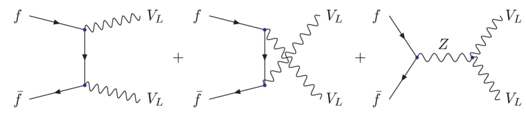
Figure 1: Feynman diagrams that contribute to the amplitude for $f\bar{f}\to V_{L}V_{L}$ in unitary gauge. The middle diagram is absent if $V=W$; the last diagram is absent if $V=Z$.

However, Eq. (7) is not the strongest upper bound that one can derive, given the above framework. By considering $f_{\pm}\bar{f}_{\pm}\to V_{L}\cdots V_{L}$, with $n$ particles in the final state, one obtains an upper bound on the scale of fermion mass generation proportional to $(v^{n}/m_{f})^{1/(n-1)}$. For arbitrarily large $n$, one obtains an upper bound arbitrarily close to the weak scale $v$ for any value of $m_{f}$. We first derive this result, then discuss its implications.

The easiest way to derive this result is to consider the theory in the limit that the weak gauge coupling goes to zero, with $v$ fixed. In this limit the weak vector bosons become massless, and the longitudinal weak vector bosons are represented by the Goldstone bosons $s^{\pm},\chi$ contained in the field $\Sigma=\exp(i\sigma\cdot\pi/v)$, where $s^{\pm}=-(\pi^{1}\mp i\pi^{2})/\sqrt{2},\chi=-\pi^{3}$. The terms that grow with energy in the amplitudes are independent of the weak gauge coupling, so they survive in this limit. Thus the high-energy behavior of amplitudes with longitudinal weak vector bosons in the final state may be obtained from the amplitudes with the vector bosons replaced with the corresponding Goldstone bosons [times a factor of $i$ ($-i$) for each outgoing (incoming) longitudinal weak vector boson]. This is the Goldstone-boson equivalence theorem [1, 14, 16, 17].

The fermion interacts with the Goldstone bosons via the interaction of Eq. (6). Expanding the $\Sigma$ field in powers of the Goldstone-boson fields, we obtain an interaction such as that shown in Fig. 2, with $n$ external Goldstone bosons. The Feynman rule for this interaction is proportional to $m_{f}/v^{n}$. The amplitude for $f_{\pm}\bar{f}_{\pm}\to\pi\cdots\pi$ is therefore proportional to $m_{f}\sqrt{s}/v^{n}$. The relevant unitarity condition on this inelastic amplitude is

$$\sigma_{inel}(2\to n)\leq\frac{4\pi}{s}\;,$$ (8)

where $\sigma_{inel}(2\to n)$ is the total cross section for $f_{\pm}\bar{f}_{\pm}\to\pi\cdots\pi$. This condition is derived in Appendix A. Since the phase space for an $n$-particle final state is proportional to $s^{n-2}$ at high energies, one finds that the unitarity condition, Eq. (8), is violated at an energy proportional to $(v^{n}/m_{f})^{1/(n-1)}$, as stated above.

Figure 2: Feynman diagram for the interaction of a fermion with $n$ Goldstone bosons.

We see that $f_{\pm}\bar{f}_{\pm}\to V_{L}\cdots V_{L}$, with $n>2$ particles in the final state, leads to a stronger upper bound than Eq. (7), which is based on the case $n=2$. Thus the Appelquist-Chanowitz bound is subsumed by this stronger bound, which is of order the weak scale, $v$, for $n$ large, independently of $m_{f}$. Since we already know that there must be new physics at the weak scale, namely the physics of electroweak symmetry breaking, the consideration of fermion-antifermion scattering into longitudinal weak vector bosons does not reveal an additional scale. This claim is supported by the fact the upper bound is independent of the fermion mass. Thus there is no upper bound on the scale of fermion mass generation.

4 Standard model

The derivation in the previous section of $f_{\pm}\bar{f}_{\pm}\to V_{L}\cdots V_{L}$, with $n$ particles in the final state, tacitly assumes that the longitudinal weak vector bosons are weakly-coupled degrees of freedom. As discussed in Section 2, this is not true in general above $\Lambda_{EWSB}\approx\sqrt{8\pi}v$. In order to justify the calculation of $f_{\pm}\bar{f}_{\pm}\to V_{L}\cdots V_{L}$ above $\Lambda_{EWSB}$, one must specify the mechanism of electroweak symmetry breaking such that the longitudinal weak vector bosons remain weakly-coupled degrees of freedom above $\Lambda_{EWSB}$. The unique theory that contains longitudinal weak vector bosons as weakly-coupled degrees of freedom to arbitrarily-high energies is the standard model, with a Higgs boson [13, 14, 15]. In this section we consider the scale of fermion mass generation in the standard model.

First consider the model envisioned in Ref. [2], in which the weak-vector-boson masses are generated via an explicit model of spontaneous symmetry breaking, but fermions are given bare masses. As an example of this, one could imagine the standard Higgs model, but with the fermion Yukawa interactions replaced by bare fermion masses, Eq. (5). However, even in this scenario, the considerations of the previous section continue to apply. The calculation of $f_{\pm}\bar{f}_{\pm}\to V_{L}\cdots V_{L}$, with $n$ particles in the final state, continues to violate unitarity at the scale of electroweak symmetry breaking for large $n$. Thus unitarity of this process does not reveal an additional scale beyond that of electroweak symmetry breaking.

The theory that is valid above the scale of electroweak symmetry breaking necessarily has a linearly-realized gauge invariance. Thus the fermion mass, Eq. (6), must be described by a Yukawa interaction

$${\cal L}=-y_{f}{\overline{F}_{L}}\phi f_{R}+H.c.\;.$$ (9)

This Lagrangian contains a Yukawa interaction of the fermion with the Higgs boson and yields the diagram in Fig. 3. This diagram, when added to the diagrams in Fig. 1, cancels the term that grows linearly with energy, leaving behind terms that fall like an inverse power of energy at high energy. A similar cancellation occurs for all processes of the type $f_{\pm}\bar{f}_{\pm}\to V_{L}\cdots V_{L}$.

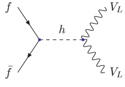
Figure 3: Additional diagram involving the exchange of a Higgs boson that contributes to the amplitude for $f\bar{f}\to V_{L}V_{L}$. This diagram cancels the terms that grow with energy resulting from the diagrams in Fig. 1.

It is tempting to identify the scale of fermion mass generation with the energy at which the amplitude for $f_{\pm}\bar{f}_{\pm}\to V_{L}V_{L}$ ceases to grow with energy, namely the Higgs mass. However, the Higgs mass is the scale of electroweak symmetry breaking, not the scale of fermion mass generation. The reason the amplitude for $f_{\pm}\bar{f}_{\pm}\to V_{L}V_{L}$ grows with energy below the Higgs mass is because the fermion mass is described in a theory with a nonlinearly-realized gauge invariance, Eq. (6). Above the Higgs mass, the amplitude for $f_{\pm}\bar{f}_{\pm}\to V_{L}V_{L}$ falls off with energy and unitarity is respected at all energies. Thus, in the standard model there is no scale associated with fermion mass generation. We will support this claim by considering extensions of the standard model in which there is a well-defined scale of fermion mass generation. These models are discussed in Sections 5 and 6.

A possible way to circumvent the above arguments is to introduce a Higgs doublet field, such that longitudinal weak vector bosons are weakly coupled above the weak scale, but to forbid the Higgs field from coupling to fermions. This can be arranged, for example, by imposing the discrete symmetry $\phi\to-\phi$. However, this also has the consequence of forbidding a gauge-invariant mass for the fermion, so the scale of fermion mass generation is moot. One might also consider a model with two Higgs doublets where only one doublet couples to fermions. Such a model is discussed in Section 7.

In this section we have argued that there is no scale of fermion mass generation in the standard model. However, Yukawa couplings are not asymptotically free in general, so the energy at which a Yukawa coupling becomes strong also indicates an upper bound on the scale of fermion mass generation. In the standard model, only the top-quark Yukawa coupling is not asymptotically free; all other Yukawa couplings are asymptotically free by virtue of the fermion’s gauge interactions. The top-quark’s Yukawa coupling is sufficiently large that it eventually overwhelms the gauge interactions, causing it to become strong at high energies. However, for $m_{t}=175$ GeV, the energy at which the top-quark’s Yukawa coupling becomes strong is many orders of magnitude above the Planck scale and is therefore irrelevant. If a quark of mass in excess of about 225 GeV existed, its Yukawa coupling would become strong below the grand-unification scale [19, 20, 21, 22].

5 Majorana neutrinos

Neutrinos are exactly massless in the standard model. However, recent observations of neutrino oscillations indicate that neutrinos have a small mass. We assume that neutrino masses are Majorana, unlike the other known fermions, which carry electric charge and are therefore forbidden to have Majorana masses. If there is no $SU(2)_{L}\times U(1)_{Y}$-singlet fermion field $\nu_{R}$ in nature, then neutrino masses are necessarily Majorana. However, even if such a field exists, the gauge symmetry allows the Majorana mass term ${\cal L}=-(M_{R}/2)\nu_{R}^{T}C\nu_{R}+H.c.$ for this field, and there is no reason why this mass should be small. Other known fermions acquire a mass only after $SU(2)_{L}\times U(1)_{Y}$ is broken, and thus their masses are of order the weak scale, $v$, or less. Since a Majorana mass for the $\nu_{R}$ field is not protected by the gauge symmetry, it is natural to assume that it would be much greater than the weak scale [23]. So even if the $\nu_{R}$ field exists, it is likely to be heavy, in which case the light neutrinos are Majorana fermions.

We have recently shown that an upper bound on the scale of Majorana-neutrino mass generation may be derived by considering the process $\nu_{\pm}\nu_{\pm}\to V_{L}V_{L}$, as shown in Fig. 4 [6]. This bound is similar to the Appelquist-Chanowitz bound on Dirac-fermion mass generation, Eq. (7), which is invalid for standard-model fermions, as we have argued in the previous two sections. Here we reconsider the upper bound on the scale of Majorana-neutrino mass generation and show that it is valid.

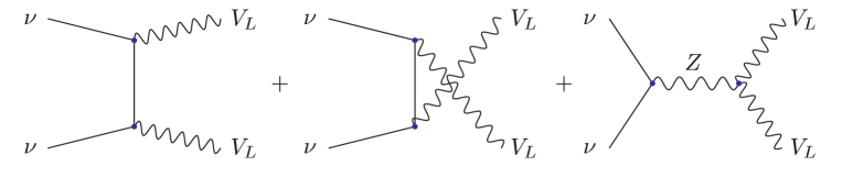
Figure 4: Feynman diagrams that contribute to the amplitude for $\nu\nu\to V_{L}V_{L}$ in unitary gauge. The last diagram is absent if $V=Z$.

As with the case of Dirac fermions, the upper bound on the scale of Majorana-neutrino mass generation was obtained by considering the process $\nu_{\pm}\nu_{\pm}\to V_{L}V_{L}$ in the absence of any diagrams involving the exchange of a Higgs boson. This is because the Majorana-neutrino mass was introduced via a bare mass term,

$${\cal L}=-\frac{1}{2}m_{\nu}\nu_{L}^{T}C\nu_{L}+H.c.\;,$$ (10)

where $C$ is the charge-conjugation matrix. However, by considering $\nu_{\pm}\nu_{\pm}\to V_{L}\cdots V_{L}$, with $n$ particles in the final state, one finds that unitarity is violated at the weak scale, $v$, for $n$ large, independently of the neutrino mass. This is analogous to the situation for Dirac fermions discussed in Section 3. Thus there is no additional upper bound, beyond that on electroweak symmetry breaking, implied by considering Majorana neutrinos scattering into longitudinal weak vector bosons when the neutrino mass is introduced via a bare mass term, Eq. (10).

In order to discover a new scale from the consideration of $\nu_{\pm}\nu_{\pm}\to V_{L}V_{L}$, one must allow the neutrino to acquire a mass by coupling to the Higgs boson. This has two consequences. First, the longitudinal weak vector bosons remain weakly coupled up to arbitrarily high energies, justifying the calculation of the diagrams in Fig. (4). Second, the process $\nu_{\pm}\nu_{\pm}\to V_{L}\cdots V_{L}$, with $n$ particles in the final state, does not lead to a stronger bound than the case with $n=2$. If the neutrino instead acquires its mass some other way, then the considerations of this section do not apply. This case is treated in Section 8.

Above the scale of electroweak symmetry breaking, the Majorana-neutrino mass must be described by a gauge-invariant term in the Lagrangian. In the Higgs model, the lowest-dimension term available is the dimension-five interaction [24]

$${\cal L}=\frac{c}{M}(L^{T}\epsilon\phi)C(\phi^{T}\epsilon L)+H.c.\;,$$ (11)

where $L=(\nu_{L},\ell_{L})$ is an $SU(2)_{L}$ doublet containing the left-chiral neutrino and charged-lepton fields and $\epsilon\equiv i\sigma_{2}$. We will show that the scale $M$ may be interpreted as the scale of Majorana-neutrino mass generation; $c$ is a dimensionless constant. This term gives rise to a Majorana-neutrino mass $m_{\nu}=cv^{2}/M$ when the neutral component of the Higgs field acquires a vacuum-expectation value $\langle\phi^{0}\rangle=v/\sqrt{2}$. It also yields a Yukawa coupling of the Majorana neutrino to the Higgs boson, thereby generating the additional contribution to the amplitude $\nu_{\pm}\nu_{\pm}\to V_{L}V_{L}$ shown in Fig. 5. However, this diagram does not cancel the terms that grow with energy, in contrast to the case of standard-model Dirac fermions. Thus the upper bound on the scale of Majorana-neutrino mass generation derived in Ref. [6] is parametrically correct, although it did not include the contribution from the Higgs-exchange diagram in Fig. 5.

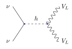
Figure 5: Additional diagram involving the exchange of a Higgs boson that contributes to the amplitude for $\nu\nu\to V_{L}V_{L}$. This diagram cancels the term that grows with energy resulting from the diagrams in Fig. 4 if $V=W$, but not if $V=Z$.

Since the Higgs boson is present at energies above the scale of electroweak symmetry breaking, one finds that there is another amplitude that grows with energy, $\nu_{\pm}\nu_{\pm}\to hh$, as shown in Fig. 6. Only the last diagram contributes to the term that grows with energy, yielding the zeroth-partial-wave amplitude (for $\sqrt{s}\gg m_{\nu},m_{h}$)

$$a_{0}\left(\frac{1}{\sqrt{2}}\nu_{\pm}\nu_{\pm}\to\frac{1}{\sqrt{2}}hh\right)\sim\mp\frac{c\sqrt{s}}{16\pi M}\sim\mp\frac{m_{\nu}\sqrt{s}}{16\pi v^{2}}\;,$$ (12)

where the relation $m_{\nu}=cv^{2}/M$ was used to obtain the final expression. This process grows with energy because the interaction responsible for the last diagram in Fig. 6, Eq. (11), has a coefficient with dimensions of an inverse power of mass. In contrast, the processes involving longitudinal weak vector bosons in the final state grow with energy due to the longitudinal polarization vectors, $\epsilon^{\mu}\approx p^{\mu}/M_{V}$ (for $p^{0}\gg M_{V}$).

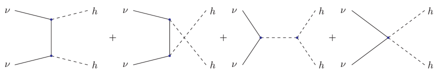
Figure 6: Feynman diagrams that contribute to the amplitude for $\nu\nu\to hh$. Only the last diagram grows with energy.

However, there is a sense in which all processes that grow with energy are related to the dimension-five interaction of Eq. (11). This can be made manifest by using the Goldstone-boson equivalence theorem, where the Goldstone bosons $s^{\pm},\chi$ are contained in the Higgs doublet, $\phi=(-is^{+},(h+v+i\chi)/\sqrt{2})$. The terms that grow with energy in the Goldstone-boson amplitudes all come from the interaction of Eq. (11), such as the last diagram in Fig. 6. It is in this sense that all processes that grow with energy are related to this dimension-five interaction.

The high-energy behavior of the amplitudes that grow with energy are collected in Appendix B. The strongest upper bound on the scale of Majorana-neutrino mass generation is obtained by applying the inelastic unitarity condition $|a_{0}|\leq 1/2$ to the amplitude

$$a_{0}\left(\frac{1}{2}(\nu_{i+}\nu_{i+}-\nu_{i-}\nu_{i-})\to\frac{1}{2}(Z_{L}Z_{L}+hh)\right)\sim-\frac{m_{\nu_{i}}\sqrt{s}}{8\pi v^{2}}\;.$$ (13)

This yields the upper bound on the scale of Majorana-neutrino mass generation

$$\Lambda_{Maj}\equiv\frac{4\pi v^{2}}{m_{\nu}}\;.$$ (14)

This equation supersedes Eq. (10) of Ref. [6]. The upper bounds on $\Lambda_{Maj}$ implied by a variety of neutrino-oscillation experiments are listed in Table 1.

Table 1: Neutrino mass-squared differences from a variety of neutrino oscillation experiments, and their interpretations. They imply a lower bound of $m_{\nu}\geq\sqrt{\Delta m^{2}}$ on the mass of one of the two participating neutrino species. The last column lists the corresponding upper bounds on $\Lambda_{Maj}$, Eq. (14), which is the upper bound on the scale of Majorana-neutrino mass generation.

Experiment	Fav’d Channel(s)	$\Delta m^{2}$ ($\rm eV^{2}$)	$\Lambda_{Maj}$ $({\rm GeV})<$
LSND [25]	$\bar{\nu}_{\mu}\to\bar{\nu}_{e}$	$0.2-2.0$	$1.7\times 10^{15}$
Atmospheric [26]	$\nu_{\mu}\to\nu_{\tau}$	$(1.6-4)\times 10^{-3}$	$1.9\times 10^{16}$
Solar [27]
MSW (LMA)	$\nu_{e}\to\nu_{\mu}$ or $\nu_{\tau}$	$(2-10)\times 10^{-5}$	$1.7\times 10^{17}$
MSW (SMA)	$\nu_{e}\to$ anything	$(3-8)\times 10^{-6}$	$4.4\times 10^{17}$
MSW (LOW)	$\nu_{e}\to\nu_{\mu}$ or $\nu_{\tau}$	$7.6\times 10^{-8}$	$2.8\times 10^{18}$
Vacuum	$\nu_{e}\to$ anything	$1.4\times 10^{-10}$	$6.4\times 10^{19}$
Just So2	$\nu_{e}\to$ anything	$5.5\times 10^{-12}$	$3.2\times 10^{20}$

In Ref. [6] we discussed two models that can saturate the upper bound on the scale of Majorana-neutrino mass generation, Eq. (14): the “see-saw” model and a Higgs-triplet model. We first review the see-saw model [28, 29]. In this model, the dimension-five interaction of Eq. (11) is replaced by the renormalizable interactions

$${\cal L}=-y_{D}\overline{L}\epsilon\phi^{*}\nu_{R}-\frac{1}{2}M_{R}\nu_{R}^{T}C\nu_{R}+H.c.\;,$$ (15)

where $\nu_{R}$ is an $SU(2)_{L}\times U(1)_{Y}$-singlet fermion field. This field has a Majorana mass term allowed by the gauge symmetry, so it is natural to expect that $M_{R}\gg v$. The first term yields a Dirac mass of $m_{D}=y_{D}v/\sqrt{2}$. The mass eigenstates of this model are a light Majorana neutrino $\nu\approx\nu_{L}$, of mass $m_{\nu}\approx m_{D}^{2}/M_{R}$, and a heavy Majorana neutrino $N\approx\nu_{R}$, of approximate mass $M_{R}$. The fact that $m_{\nu}\ll m_{D}$ provides an attractive explanation for why neutrinos are so much lighter than the other known (Dirac) fermions. At energies above the mass of the heavy neutrino, $M_{R}$, the Feynman diagrams for $\nu_{\pm}\nu_{\pm}\to Z_{L}Z_{L}$ in Figs. 4 and 5 are augmented by diagrams in which the heavy neutrino is exchanged in the $t$- and $u$-channels. These diagrams cancel all terms that grow with energy. The process $\nu_{\pm}\nu_{\pm}\to hh$ also ceases to grow with energy, because the last diagram in Fig. 6, which was responsible for the term that grows with energy, is not present. It is replaced by diagrams, similar to the first two diagrams in that figure, with the exchange of $N$ in the $t$- and $u$-channels. Thus the scale of Majorana-neutrino mass generation in the see-saw model is the mass of the heavy neutrino, $M_{R}$. This is because the Lagrangian above $M_{R}$, Eq. (15), is renormalizable.

Below $M_{R}$, one integrates out the field $\nu_{R}$ and obtains the nonrenormalizable interaction of Eq. (11), with $c/M=-y_{D}^{2}/2M_{R}$. Thus we associate the scale $M$ with $M_{R}$, which is the scale of Majorana-neutrino mass generation in this model, and $c=-y_{D}^{2}/2$. The mass of the heavy neutrino, $M_{R}\approx m_{D}^{2}/m_{\nu}\approx y_{D}^{2}v^{2}/2m_{\nu}$, saturates (within a factor of order unity) the upper bound on the scale of Majorana-neutrino mass generation, Eq. (14), when the Yukawa coupling takes its largest allowed value, $y_{D}\;{\raise 1.29167pt\hbox{$<$\kern-7.5pt\lower 4.30554pt\hbox{$\sim$}}}\;\sqrt{8\pi}$ [30, 31, 32].

The Higgs-triplet model [33, 34, 35, 36, 37] introduces an SU(2)_L-triplet, $Y=1$ Higgs field, $\Phi^{i}$, and the renormalizable interaction

$${\cal L}=-y_{M}L^{T}\epsilon\sigma^{i}CL\Phi^{i}+H.c.\;,$$ (16)

which replaces the dimension-five interaction of Eq. (11). The usual Higgs doublet field is also present in the model. The vacuum-expectation value of the Higgs triplet field must be much less than the weak scale, because the relation $M_{W}^{2}\simeq M_{Z}^{2}\cos^{2}\theta_{W}$, which is satisfied experimentally, is obtained if the weak bosons acquire their mass dominantly from the vacuum-expectation value of an SU(2)_L doublet, but not a triplet. The interaction of Eq. (16) generates a small Majorana-neutrino mass, $m_{\nu}=2y_{M}u$, when the neutral component of the Higgs field, $\Phi^{0}=(\Phi^{1}+i\Phi^{2})/\sqrt{2}$, acquires a small vacuum-expectation value $\langle\Phi^{0}\rangle=u/\sqrt{2}$. This model contains three neutral scalars, one singly-charged scalar, and one doubly-charged scalar. The term of Eq. (16) gives rise to new interactions that yield the additional Feynman diagrams in Fig. 7 involving these Higgs scalars in the intermediate state. The first diagram cancels the terms that grow with energy in $\nu_{\pm}\nu_{\pm}\to V_{L}V_{L}$, the second diagram cancels the term that grows with energy in $\ell_{-}\nu_{-}\to W_{L}^{-}Z_{L}$, and the third diagram cancels the term that grows with energy in $\ell_{-}\ell_{-}\to W_{L}^{-}W_{L}^{-}$. The process $\nu_{\pm}\nu_{\pm}\to hh$ also ceases to grow with energy because the last diagram in Fig. 6, which was responsible for the term that grows with energy, is eliminated and replaced by a diagram analogous to the first diagram of Fig. 7 (with the $V_{L}$ replaced by $h$). Thus the scale of Majorana-neutrino mass generation is the mass of these Higgs scalars. This is because the theory above the mass of these scalars, Eq. (16), is renormalizable.

The Higgs potential of the model is discussed in Appendix C. The triplet field has a mass term allowed by the gauge symmetry, ${\cal L}=-M_{T}^{2}\Phi^{i*}\Phi^{i}$, so it is natural for it to be much heavier than the weak scale, in which case the Higgs scalars $H^{0},H^{-},H^{--}$ have masses of approximately $M_{T}$. The unique renormalizable term in the potential linear in the triplet field is ${\cal L}=-M_{3}\phi^{T}\epsilon\sigma^{i}\phi\Phi^{i*}+H.c.$ In the limit $M_{T}\gg v$, the vacuum-expectation value of the triplet field is $u\approx M_{3}v^{2}/M_{T}^{2}$, which is much less than $v$. Since the Majorana neutrino mass is $m_{\nu}=2y_{M}u$, this model provides a natural explanation of why neutrino masses are light. Solving for the mass of the heavy Higgs scalars in terms of the neutrino mass, one obtains $M_{T}\approx 2(M_{3}/M_{T})y_{M}v^{2}/m_{\nu}$. This respects the upper bound on the scale of Majorana-neutrino mass generation, Eq. (14), since $M_{3}/M_{T}\;{\raise 1.29167pt\hbox{$<$\kern-7.5pt\lower 4.30554pt\hbox{$\sim$}}}\;\sqrt{\pi}$ (see Appendix C) and $y_{M}\;{\raise 1.29167pt\hbox{$<$\kern-7.5pt\lower 4.30554pt\hbox{$\sim$}}}\;\sqrt{2\pi}$ (the analogue of $y_{D}\;{\raise 1.29167pt\hbox{$<$\kern-7.5pt\lower 4.30554pt\hbox{$\sim$}}}\;\sqrt{8\pi}$ mentioned in the previous section). The bound is saturated (within a factor of order unity) when both $M_{3}/M_{T}$ and $y_{M}$ attain their maximum values.

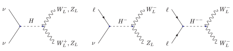
Figure 7: Additional diagrams that contribute when the Majorana neutrino acquires its mass via a coupling to an SU(2)_L-triplet Higgs field.

Below the mass of the heavy Higgs scalars, $M_{T}$, one integrates out the Higgs triplet field and obtains the dimension-five interaction of Eq. (11), with $c/M=2M_{3}y_{M}/M_{T}^{2}$. Since we associate $M$, the scale of Majorana-neutrino mass generation, with $M_{T}$, we are left with $c=2M_{3}y_{M}/M_{T}$.

The study of these two models leads us to the following definition: The scale of fermion mass generation is the minimum energy at which the fermion mass is generated by a renormalizable interaction. In the standard model the fermion mass is generated by a renormalizable interaction at all energies (above the Higgs mass), so there is no scale of fermion mass generation.

6 Fermions in non-standard representations

With the fermion content of the standard model, the only fermions that do not acquire their mass from a renormalizable interaction with the Higgs field are Majorana neutrinos, Eq. (11). In this section we extend the fermion content of the standard model to include fermions in nonstandard representations of $SU(2)_{L}\times U(1)_{Y}$, such that they acquire Dirac masses from nonrenormalizable interactions. This will demonstrate that the results obtained for Majorana neutrinos in the previous section are not peculiar to the Majorana nature of the fermions. Furthermore, by choosing the fermion representation appropriately, we will be able to construct interactions of arbitrary dimension to generate the fermion mass. This will allow us to study the consequences of unitarity in a more general setting.

Consider adding an $SU(2)_{L}$-triplet, $Y=-1$ fermion field $F_{L}^{\alpha\beta}$ and an $SU(2)_{L}$-singlet, $Y=-2$ fermion field $f_{R}^{--}$ to the standard model. As it stands, this model has gauge and gravitational anomalies; however, it is possible to embed this model in an anomaly-free model, as demonstrated explicitly in Appendix D. The lowest-dimension interaction that couples these fermions to the Higgs field ($Y=1/2$) is

$${\cal L}=-\frac{c}{M}{\overline{F}_{L}}^{\alpha\beta}\phi^{\alpha}\phi^{\beta}f_{R}^{--}+H.c.\;,$$ (17)

which is the analogue of Eq. (9), but is of dimension five, like Eq. (11). The $SU(2)_{L}$-triplet field can be represented by a symmetric two-index tensor in $SU(2)_{L}$ space,

$$F_{L}^{\alpha\beta}\equiv\left(\begin{array}[]{cc}f_{L}^{0}&\frac{1}{\sqrt{2}}f_{L}^{-}\\ \frac{1}{\sqrt{2}}f_{L}^{-}&f_{L}^{--}\end{array}\right)\;.$$ (18)

This Lagrangian gives rise to a Dirac mass $m_{f}=cv^{2}/2M$ for the field $f^{--}$ when the neutral component of the Higgs field acquires a vacuum-expectation value $\langle\phi^{0}\rangle=v/\sqrt{2}$.

The Feynman diagrams for the amplitude $f^{--}_{\pm}f^{++}_{\pm}\to V_{L}V_{L}$ are similar to those in Figs. (1) and (3). However, the $s$-channel Higgs diagram of Fig. (3) does not cancel the term that grows with energy, in contrast to the case of standard-model Dirac fermions. Thus the situation is analogous to the case of Majorana neutrinos discussed in the previous section. This demonstrates that the results obtained there were not peculiar to the Majorana nature of the fermions, but instead stem from the fact that the fermion mass is generated by a dimension-five interaction.

As in the previous section, one can use the Goldstone-boson equivalence theorem to calculate the high-energy behavior of the amplitude for $f^{--}_{\pm}f^{++}_{\pm}\to V_{L}V_{L}$ (as well as the amplitude with one $V_{L}$ replaced by $h$). The terms that grow with energy all come from the dimension-five interaction, Eq. (17). This interaction yields a Feynman diagram similar to the last diagram in Fig. 6. The resulting amplitude is proportional to $c\sqrt{s}/M\approx m_{f}\sqrt{s}/v^{2}$, as in the case of Majorana neutrinos. The strongest upper bound on the scale of fermion mass generation comes from applying the inelastic unitarity condition $|a_{0}|\leq 1/2$ to the amplitude

$$a_{0}\left(\frac{1}{\sqrt{2}}(f^{--}_{+}f^{++}_{+}-f^{--}_{-}f^{++}_{-})\to\frac{1}{2}(Z_{L}Z_{L}+hh)\right)\sim-\frac{m_{f}\sqrt{s}}{4\pi\sqrt{2}v^{2}}\;,$$ (19)

which is the analogue of Eq. (13). This yields the upper bound on the scale of Dirac-fermion mass generation

$$\Lambda_{5}\equiv\frac{4\pi v^{2}}{\sqrt{2}m_{f}}\;,$$ (20)

where the subscript indicates that the Dirac fermion mass is generated by a dimension-five interaction, Eq. (17). This is the analogue of Eq. (14).

One can generalize this analysis to an interaction of arbitrary dimension as follows. Consider the standard model with the addition of an $SU(2)_{L}$ $(n+1)$-plet, $F_{L}^{\alpha\cdots\beta}$, with $n$ totally symmetric indices. Also add an $SU(2)_{L}$-singlet field $f_{R}^{Q}$ of hypercharge (and electric charge) $Q$. The lowest-dimension interaction that generates a Dirac mass is the dimension-$d$ interaction

$${\cal L}=-\frac{c}{M^{d-4}}{\overline{F}_{L}}^{\alpha\cdots\beta}\phi^{\alpha}\cdots\phi^{\beta}f_{R}^{Q}+H.c.\;,$$ (21)

where $d=n+3$. The fields $F_{L}^{2\cdots 2}\equiv f_{L}^{Q}$ and $f_{R}^{Q}$ form a Dirac mass term of mass $m_{f}=c(v/\sqrt{2})^{d-3}/M^{d-4}$ when the neutral component of the Higgs field acquires a vacuum-expectation value $\langle\phi^{0}\rangle=v/\sqrt{2}$.

Applying the unitarity condition $|a_{0}|\leq 1/2$ to the amplitude for $f^{Q}_{\pm}\bar{f}^{Q}_{\pm}\to V_{L}V_{L}$ (most easily calculated using the Goldstone-boson equivalence theorem) again yields an upper bound on the scale of fermion mass generation that is proportional to $v^{2}/m_{f}$, like Eq. (20). However, the strongest upper bound on the scale of fermion mass generation comes not from this process, but instead from $f^{Q}_{\pm}\bar{f}^{Q}_{\pm}\to h\cdots h$, with $n=d-3$ Higgs bosons in the final state. The relevant Feynman diagram, shown in Fig. 8, is generated from the dimension-$d$ interaction of Eq. (21). The unitarity condition on this inelastic amplitude is given in Eq. (8), where $\sigma_{inel}(2\to n)$ is the total cross section for $f^{Q}_{\pm}\bar{f}^{Q}_{\pm}\to h\cdots h$. The strongest bound on the scale of fermion mass generation is obtained by considering the initial state $(f^{Q}_{+}\bar{f}^{Q}_{+}\mp f^{Q}_{-}\bar{f}^{Q}_{-})/\sqrt{2}$, and summing over the cross sections obtained by replacing an even (upper sign) or odd (lower sign) number of $h$’s in the final state with $Z_{L}$’s (or, via the equivalence theorem, $\chi$’s). Hence, for a Dirac fermion whose mass is generated via the dimension-$d$ interaction of Eq. (21), the upper bound on the scale of fermion mass generation is

$$\Lambda_{d}\equiv 4\pi\kappa_{d}\left(\frac{v^{d-3}}{m_{f}}\right)^{1/(d-4)}\;,$$ (22)

where $\kappa_{d}$, given in Eq. (84), is a number of order unity. We derive this result in Appendix E. The results for $\Lambda_{d}$ are listed in Table 2 for a few values of $d$.

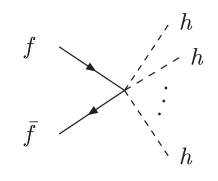
Figure 8: Feynman diagram for the interaction of a fermion with $n$ Higgs bosons.

The scale $M$ has the natural interpretation as the energy at which the effective field theory involving the dimension-$d$ interaction of Eq. (21) is subsumed by a deeper theory. For example, $M$ corresponds to the mass of the heavy neutrino in the see-saw model discussed in Section 5. Since the fermion acquires a mass $m_{f}=c(v/\sqrt{2})^{d-3}/M^{d-4}$ from the dimension-$d$ interaction, the scale $M$ is related to the fermion mass by

$$M=\left(\frac{c}{m_{f}}\left(\frac{v}{\sqrt{2}}\right)^{d-3}\right)^{1/(d-4)}\;.$$ (23)

Thus $M$ respects the upper bound on the scale of fermion mass generation, Eq. (22), provided that $c\leq\sqrt{2}(4\pi\sqrt{2}\kappa_{d})^{d-4}$. This condition corresponds to the convergence of the energy expansion, based on the interaction of Eq. (21), for $E\;{\raise 1.29167pt\hbox{$<$\kern-7.5pt\lower 4.30554pt\hbox{$\sim$}}}\;M$.

Table 2: Upper bound on the scale of fermion mass generation, $\Lambda_{d}$, for Dirac fermions that acquire a mass via the dimension-$d$ interaction of Eq. (21).

$d$	$\Lambda_{d}$
4	$\infty$
5	$\frac{4\pi}{\sqrt{2}}\frac{v^{2}}{m_{f}}$
6	$\frac{4\pi}{6^{1/4}}\left(\frac{v^{3}}{m_{f}}\right)^{1/2}$
$\vdots$	$\vdots$
$d$	$4\pi\kappa_{d}\left(\frac{v^{d-3}}{m_{f}}\right)^{1/(d-4)}$

7 Higher-dimension interactions

In the standard model, Dirac fermions acquire mass via a dimension-four interaction with the Higgs field, Eq. (9). As we argued in Section 4, there is no scale of fermion mass generation in the standard model. However, it is likely that the standard model is supplemented by higher-dimensions interactions, whose presence has not yet been revealed to us due to the insufficient energy and/or accuracy of our experiments. In this section we consider the implications of higher-dimension interactions on the scale of Dirac-fermion mass generation in the standard model. Our discussion applies to all models that reduce to the standard model when the mass of the physics beyond the standard model is taken to infinity (decoupling).

The lowest-dimension interaction available to supplement the standard model is of dimension five. With the usual fermion content (no $\nu_{R}$ field), there is only one such interaction, which we already encountered in Eq. (11). This interaction gives rise to a Majorana mass for the neutrino, but no other fermion masses. Thus we must consider interactions of at least dimension six in the case of Dirac fermions.

In contrast with interactions of dimension five, there are a large number of interactions of dimension six available with the field content of the standard model [38]. However, there is only one that contributes to fermion masses, given by

$${\cal L}=-\frac{c}{M^{2}}{\overline{F}_{L}}\phi f_{R}\phi^{\dagger}\phi+H.c.\;,$$ (24)

which was already considered by Golden [3]. This interaction, in concert with the usual dimension-four interaction of Eq. (9), yields a Dirac fermion mass, when the neutral component of the Higgs field acquires a vacuum-expectation value $\langle\phi^{0}\rangle=v/\sqrt{2}$, of

$$m_{f}=y_{f}\frac{v}{\sqrt{2}}+\frac{c}{M^{2}}\left(\frac{v}{\sqrt{2}}\right)^{3}\;.$$ (25)

This interaction also affects the coupling of the Higgs boson to the fermion, thereby affecting the contribution of the diagram in Fig. 3 to $f\bar{f}\to V_{L}V_{L}$. The resulting zeroth-partial-wave amplitude grows with energy like

$$a_{0}\left(f_{\pm}\bar{f}_{\pm}\to V_{L}V_{L}\right)\approx\frac{c}{M^{2}}v\sqrt{s}\;,$$ (26)

which exceeds the unitarity bound at an energy of order

$$\Lambda\approx\frac{M^{2}}{cv}\approx\frac{v^{2}}{m_{f}-y_{f}v/\sqrt{2}}\;,$$ (27)

where we have used Eq. (25). This is an upper bound on the scale of new physics.

In the standard model, where $m_{f}=y_{f}v/\sqrt{2}$, the upper bound on the scale of new physics implied by Eq. (27) is infinity. For Eq. (27) to imply a scale of new physics, one would need to know not only that the fermion has a mass $m_{f}$, but also that the dimension-four Yukawa coupling of the fermion, Eq. (9), differs from the standard-model value $y_{f}=\sqrt{2}m_{f}/v$. Let us imagine that this Yukawa coupling were very small, such that the fermion acquires its mass dominantly from the dimension-six interaction in Eq. (24). The upper bound on the scale of new physics implied by Eq. (27) is then proportional to $v^{2}/m_{f}$.

However, as we saw in the previous section, when a fermion acquires a mass via a dimension-six interaction, a stronger upper bound can be obtained by considering the unitarity of the process $f_{\pm}\bar{f}_{\pm}\to V_{L}V_{L}V_{L}$. One finds

$$a_{0}\left(f_{\pm}\bar{f}_{\pm}\to V_{L}V_{L}V_{L}\right)\approx\frac{c}{M^{2}}\sqrt{s}\;,$$ (28)

which exceeds the unitarity bound of Eq. (8) at an energy of order

$$\Lambda^{2}\approx\frac{M^{2}}{c}\approx\frac{v^{3}}{m_{f}-y_{f}v/\sqrt{2}}\;,$$ (29)

where we have used Eq. (25). If we imagine that the Yukawa coupling were very small, such that the fermion acquires its mass dominantly from the dimension-six interaction in Eq. (24), then the upper bound on the scale of new physics is proportional to $(v^{3}/m_{f})^{1/2}$.

In general, both the dimension-four interaction of Eq. (9) and the dimension-six interaction of Eq. (24) contribute to the fermion mass. In keeping with our definition of the scale of fermion mass generation presented at the end of Section 5, we regard Eq. (29) as an upper bound on the scale of new physics, not an upper bound on the scale of fermion mass generation. Since the fermion mass is generated in part by a renormalizable interaction at all energies (above the Higgs mass), there is no scale of fermion mass generation, as in the case of the standard model.

As a specific example of a model with a decoupling limit, consider a model with two Higgs-doublet, $Y=1$ fields, with a discrete symmetry $\phi_{1}\to-\phi_{1}$ such that only $\phi_{2}$ couples to a given fermion. The most general scalar potential for this model may be written as [39]

$$V(\phi_{1},\phi_{2}) = m_{11}^{2}\phi_{1}^{\dagger}\phi_{1}+m_{22}^{2}\phi_{2}^{\dagger}\phi_{2}-m_{12}^{2}[\phi_{1}^{\dagger}\phi_{2}+\phi_{2}^{\dagger}\phi_{1}]+\frac{1}{2}\lambda_{1}(\phi_{1}^{\dagger}\phi_{1})^{2}+\frac{1}{2}\lambda_{2}(\phi_{2}^{\dagger}\phi_{2})^{2}$$ (30)

$$+ \lambda_{3}(\phi_{1}^{\dagger}\phi_{1})(\phi_{2}^{\dagger}\phi_{2})+\lambda_{4}(\phi_{1}^{\dagger}\phi_{2})(\phi_{2}^{\dagger}\phi_{1})+\frac{1}{2}\lambda_{5}[(\phi_{1}^{\dagger}\phi_{2})^{2}+(\phi_{2}^{\dagger}\phi_{1})^{2}]\;,$$

where the $\lambda_{i}$’s are real, and where the discrete symmetry is softly broken by the term proportional to $m_{12}^{2}$. The coupling of a fermion $f$ to the Higgs field $\phi_{2}$ is given by a dimension-four Yukawa interaction

$${\cal L}=-y_{f}{\overline{F}_{L}}\phi_{2}f_{R}+H.c.\;,$$ (31)

where $F_{L}$ is an $SU(2)_{L}$-doublet fermion field whose lower component is $f_{L}$.

We study the decoupling limit in a simple way, by integrating out one of the Higgs-doublet fields. A convenient way to accomplish this is to first make a rotation in Higgs-doublet-field space such that the mass matrix is diagonal. Thus we define fields $\Phi,\phi$, given by

$$\left(\begin{array}[]{c}\Phi\\ \phi\end{array}\right)=\left(\begin{array}[]{rr}\cos\alpha&\sin\alpha\\ -\sin\alpha&\cos\alpha\end{array}\right)\left(\begin{array}[]{c}\phi_{1}\\ \phi_{2}\end{array}\right)\;,$$ (32)

where the angle $\alpha$ is chosen to eliminate the off-diagonal term in the mass matrix, proportional to $m_{12}^{2}$. The resulting scalar potential is

$$V(\phi,\Phi)=-\mu^{2}\phi^{\dagger}\phi+M^{2}\Phi^{\dagger}\Phi+\cdots+\tilde{\lambda}_{6}[(\phi^{\dagger}\phi)(\phi^{\dagger}\Phi)+H.c.]\;,$$ (33)

where we have suppressed all quartic interactions except a term, linear in $\Phi$, which is induced by the rotation in Higgs-field space. This is the unique term linear in $\Phi$; its coefficient $\tilde{\lambda}_{6}$ is a linear combination of the $\lambda_{i}$’s in Eq. (30). We now consider the decoupling limit $M^{2}\gg\mu^{2}$ and integrate out the Higgs field $\Phi$. In so doing the Yukawa interaction of Eq. (31) becomes, for energies less than $M$,

$${\cal L} = -y_{f}\cos\alpha{\overline{F}_{L}}\phi f_{R}-y_{f}\sin\alpha{\overline{F}_{L}}\Phi f_{R}+H.c.$$ (34)

$$= -y_{f}^{\prime}{\overline{F}_{L}}\phi f_{R}-\frac{c}{M^{2}}{\overline{F}_{L}}\phi f_{R}\phi^{\dagger}\phi+H.c.\;,$$

where $y_{f}^{\prime}=y_{f}\cos\alpha$ and $c=-y_{f}\tilde{\lambda}_{6}\sin\alpha$. This interaction is exactly of the form of the standard model plus the dimension-six term of Eq. (24), where $M$ is identified with the mass of the heavy Higgs field.

In Ref. [4], the decoupling limit of a two-Higgs-doublet model was studied in an attempt to find a model in which the scale of fermion mass generation saturates the Appelquist-Chanowitz bound, $\Lambda_{f}\approx v^{2}/m_{f}$. The mass of the heavy neutral Higgs scalar was identified as the scale of fermion mass generation. We instead consider it to be a scale of new physics; there is no scale of fermion mass generation since the fermion mass arises in part from a renormalizable interaction. This attempt to saturate the Appelquist-Chanowitz bound with the mass of the heavy neutral Higgs scalar failed, and instead Ref. [4] identified the upper bound on the mass of this particle to be proportional to $(v^{3}/m_{f})^{1/2}$, as one would expect if the fermion mass arose from a dimension-six interaction (see Table 2). This occurs because in the limit studied in Refs. [4, 5] one obtains $\alpha\to-\pi/2$, in which case $y_{f}^{\prime}\to 0$ in Eq. (34). The fermion mass is therefore generated by the dimension-six interaction of Eq. (34). Thus we reproduce the results of Refs. [4, 5] in a much simpler way.

It was also shown in Refs. [4, 5] that the only limit in which the mass of the heavy neutral Higgs scalar $H$ can saturate the Appelquist-Chanowitz bound, $\Lambda_{f}\approx v^{2}/m_{f}$, is if some of the quartic couplings are taken to grow with the heavy Higgs mass (nondecoupling). We show in Appendix F that the two models studied in Refs. [4] and [5] are not the same, although they both involve allowing one or more quartic couplings to grow with the heavy Higgs mass. However, these models are unphysical since the quartic couplings cannot exceed ${\cal O}(4\pi)$.

8 Models without a Higgs field

The standard model (and extensions thereof) is the unique theory in which the longitudinal weak vector bosons can be treated as weakly-coupled degrees of freedom at energies above the scale of electroweak symmetry breaking. In this section we discuss the scale of fermion mass generation in models without a Higgs field. We will see that the upper bound on the scale of fermion mass generation depends on the dimensionality of the interaction responsible for generating the fermion mass.

Above energies above $\Lambda_{EWSB}\equiv\sqrt{8\pi}v$, the longitudinal weak vector bosons cannot generally be treated as weakly-coupled degrees of freedom. As discussed in Section 3, at high energies one may think of the longitudinal weak vector bosons as Goldstone bosons via the Goldstone-boson equivalence theorem. The situation is analogous to QCD, where the pions are the Goldstone bosons of broken chiral symmetry. Consider the process $e^{+}e^{-}\to\pi^{+}\pi^{-}$. At energies less than the scale of chiral symmetry breaking, $\Lambda_{\chi SB}\approx 1$ GeV, one may treat the pions as point particles, using the effective chiral Lagrangian. However, above the scale of chiral symmetry breaking, it is invalid to treat the pions as point particles. In the same way, the electroweak model ceases to be a useful description of longitudinal weak vector bosons at energies above the scale of electroweak symmetry breaking if there is no Higgs field.

Consider fermion mass generation in a theory in which electroweak symmetry breaking is described by technicolor [41, 42]. Since the longitudinal weak vector bosons are not weakly coupled above $\Lambda_{EWSB}$, one cannot calculate amplitudes involving external longitudinal weak vector bosons perturbatively. However, one may still discuss the scale of fermion mass generation. At the weak scale the lowest-dimension interaction that generates a fermion mass is a dimension-six interaction between technifermions and ordinary fermions, which yields a fermion mass when the technifermions condense. If the coefficient of this dimension-six interaction is $c/M^{2}$, one obtains

$$m_{f}\approx c\frac{\langle\overline{T}T\rangle}{M^{2}}\;,$$ (35)

where $\langle\overline{T}T\rangle$ is the technifermion condensate. In extended technicolor (ETC), this dimension-six interaction is the low-energy approximation to the interaction of fermions and technifermions via the exchange of extended-technicolor gauge bosons of mass $M_{ETC}$ [43, 44]. Since the theory above $M_{ETC}$ is renormalizable, the scale of fermion mass generation is $M_{ETC}$. We identify $M$ with $M_{ETC}$, and $c$ with $g_{ETC}^{2}$, the square of the ETC gauge coupling. Thus one obtains from Eq. (35)

$$M_{ETC}\approx\left(g_{ETC}^{2}\frac{\langle\overline{T}T\rangle}{m_{f}}\right)^{1/2}\;.$$ (36)

In a QCD-like model $\langle\overline{T}T\rangle\approx v^{3}$. Thus Eq. (36) is the analogue of the upper bound on the scale of fermion mass generation obtained in the model of Section 6 in which a fermion acquires a mass from a dimension-six interaction, $\Lambda_{6}\approx(v^{3}/m_{f})^{1/2}$ (see Table 2).

The scale of fermion mass generation, $M$, can be increased for a fixed value of $m_{f}$ if the technifermion condensate, evaluated at $M$, is enhanced. Such is the case in walking technicolor [45, 46, 47, 48]. This may also be described in terms of the dimensionality of the operator responsible for generating the fermion mass. The composite operator $\overline{T}T$ has a large anomalous dimension, $\gamma_{m}>1$, which is assumed to be constant over the range of energies $v\;{\raise 1.29167pt\hbox{$<$\kern-7.5pt\lower 4.30554pt\hbox{$\sim$}}}\;E\;{\raise 1.29167pt\hbox{$<$\kern-7.5pt\lower 4.30554pt\hbox{$\sim$}}}\;M$. Thus the four-fermion operator responsible for generating the fermion mass has scaling dimension $6-\gamma_{m}$ over this range. The fermion mass is given by

$$m_{f}\approx c\frac{\langle\overline{T}T\rangle}{M^{2}}\left(\frac{M}{v}\right)^{\gamma_{m}}\;,$$ (37)

so the scale of fermion mass generation is related to the fermion mass by

$$M\approx\left(c\frac{v^{3-\gamma_{m}}}{m_{f}}\right)^{1/(2-\gamma_{m})}\;,$$ (38)

where we have used $\langle\overline{T}T\rangle\approx v^{3}$. This is the analogue of $\Lambda_{d}\approx(v^{d-3}/m_{f})^{1/(d-4)}$, Eq. (22), for an interaction of scaling dimension $d=6-\gamma_{m}$.

A particularly interesting case of Eq. (37) occurs when the physics at $M$ is fine tuned such that $\gamma_{m}=2$ [49, 50, 51]. In this case, the enhancement of the technifermion condensate exactly cancels the $1/M^{2}$ suppression of the four-fermion operator responsible for generating the fermion mass, leading to $m_{f}={\cal O}(v)$, independently of the value of $M$. Hence, there is no upper bound on the scale of fermion mass generation, as also follows from Eq. (38). The scaling dimension of the composite operator $\overline{T}T$ becomes $3-\gamma_{m}=1$ in this case, the same as that of a weakly-coupled scalar field. It is natural to associate this fine-tuned limit with the emergence of a light, composite scalar that acquires a small vacuum-expectation value $v\ll M$ and that has renormalizable Yukawa couplings (unsuppressed by $M$) to standard-model fermions [52]. At energies less than $M$, this composite scalar behaves like a Higgs boson, and the resulting theory reduces to the standard model when $M$ is taken to infinity (decoupling). Accordingly, the considerations of Sections 4 and 7 apply, where we concluded that there is no upper bound on the scale of fermion mass generation, in agreement with the above argument.

9 Conclusions

In this paper we studied the scale of fermion mass generation. We critically re-examined an upper bound on this scale, due to Appelquist and Chanowitz [2], obtained by considering the process $f_{\pm}\bar{f}_{\pm}\to V_{L}V_{L}$, where the subscripts on the fermions indicate helicity $\pm 1/2$, and $V_{L}=W_{L},Z_{L}$ denotes longitudinal (helicity zero) weak vector bosons. In the absence of the Higgs boson, the amplitude for this process grows with energy and violates the unitarity bound at an energy of order $\Lambda_{f}\approx v^{2}/m_{f}$. We showed that there exists a stronger bound, proportional to $(v^{n}/m_{f})^{1/(n-1)}\!$, obtained by considering the process $f_{\pm}\bar{f}_{\pm}\to V_{L}\cdots V_{L}$ with $n>2$ particles in the final state. For large $n$, this bound is arbitrarily close to the upper bound on the scale of electroweak symmetry breaking, regardless of the fermion mass. Thus there is no upper bound on the scale of fermion mass generation.

We further argued that the derivation of this bound is valid only if the longitudinal weak vector bosons are weakly coupled at energies above the scale of electroweak symmetry breaking. This requires the existence of a Higgs doublet, since the standard Higgs model (and extensions thereof that decouple when the mass of the additional physics is taken to infinity) is the unique theory in which the longitudinal weak bosons remain weakly coupled at high energy. Once the Higgs doublet is included in the theory, the upper bound on the scale of fermion mass generation depends only on the dimensionality of the operator responsible for generating the fermion mass. In the standard model, fermions acquire their mass from a dimension-four interaction with the Higgs field, which has a dimensionless Yukawa coupling. Thus there is no scale of fermion mass generation in the standard model.

Majorana neutrinos acquire their mass from an interaction of dimension five, with a coefficient with dimensions of an inverse power of mass. This mass sets the scale for Majorana-neutrino mass generation. The amplitude for $\nu_{\pm}\nu_{\pm}\to V_{L}V_{L}$ grows with energy despite the inclusion of the Higgs boson, because the neutrino acquires its mass from a nonrenormalizable interaction. Applying the unitarity condition to the amplitude, we derived an upper bound on the scale of Majorana-neutrino mass generation [6]

$$\Lambda_{Maj}\equiv\frac{4\pi v^{2}}{m_{\nu}}\;.$$ (39)

The upper bounds on $\Lambda_{Maj}$ implied by a variety of neutrino-oscillation experiments are listed in Table 1.

We considered extending the standard model by adding fermions in nonstandard representations of $SU(2)_{L}\times U(1)_{Y}$ such that they acquire a Dirac mass from an interaction of dimension $d$. We showed that the strictest upper bound on the scale of fermion mass generation is obtained by applying the unitarity condition to the amplitude for $f_{\pm}\bar{f}_{\pm}\to V_{L}\cdots V_{L}$, with $n=d-3$ particles in the final state. This upper bound is proportional to $(v^{d-3}/m_{f})^{1/(d-4)}$. For a fermion that acquires mass via the dimension-$d$ interaction of Eq. (21), the upper bound on the scale of fermion mass generation is listed in Table 2.

For a fermion that acquires its mass via an interaction of dimension four, the amplitude for $f_{\pm}\bar{f}_{\pm}\to V_{L}V_{L}$ ceases to grow with energy above the Higgs mass. This reflects the fact that the Higgs mass is the scale of electroweak symmetry breaking and that the fermion mass is generated via a renormalizable interaction. However, the Higgs mass is not the scale of fermion mass generation, as evidenced by the fact that there is no cancellation of the term that grows with energy for fermions that acquire their mass via an interaction of dimension $d>4$.

We defined the scale of fermion mass generation as the minimum energy at which the fermion mass is generated by a renormalizable interaction. In the standard model the fermion mass is generated by a renormalizable interaction at all energies (above the Higgs mass), so there is no scale of fermion mass generation.

We also considered extending the standard model by maintaining the same particle content but adding higher-dimension interactions. For fermions other than Majorana neutrinos, the lowest-dimension interaction one can add is of dimension six. There is only one dimension-six interaction that affects the fermion mass. To learn of the presence of this interaction requires knowledge not only of the fermion mass, but of its interaction with the Higgs boson. This will be a goal of future experiments once the Higgs boson is discovered. We showed that a two-Higgs-doublet model generates this dimension-six interaction when one of the Higgs doublets is taken to be heavy and is integrated out.

Finally, we considered models without a Higgs field. The process $f_{\pm}\bar{f}_{\pm}\to V_{L}V_{L}$ cannot be used to derive an upper bound on the scale of fermion mass generation because the longitudinal weak vector bosons are not weakly coupled above the scale of electroweak symmetry breaking. Nevertheless, one can discuss the scale of fermion mass generation in specific models. We showed that the relation between the fermion mass and the scale of fermion mass generation depends on the dimensionality of the interaction responsible for generating the fermion mass.

The most important conclusion of this study is that there is no upper bound on the scale of (Dirac) fermion mass generation in the standard model. This is disappointing, because an upper bound on this scale would provide a target for future accelerators, in the same way that the upper bound on the scale of electroweak symmetry breaking, $\Lambda_{EWSB}\equiv\sqrt{8\pi}v\approx 1$ TeV, provides a target for the CERN Large Hadron Collider. This does not preclude the possibility that new physics lies at accessible energies; it only says that (Dirac) fermion masses do not imply a scale of new physics. In contrast, there is an upper bound on the scale of Majorana-neutrino mass generation, Eq. (39), and although this upper bound is beyond the reach of future accelerators, the fact that the upper bounds on $\Lambda_{Maj}$ lie near the grand-unification scale (see Table 1) bolsters our belief in the relevance of grand unification for physics beyond the standard model.

Appendix A

We derive the upper bound on the inelastic $2\to n$ scattering cross section, Eq. (8), from the unitarity of the $S$ matrix, $S^{\dagger}S=1$. Writing $S=1+iT$, one obtains

$$T^{\dagger}T=2\,{\rm Im}\,T\;.$$ (40)

Take the matrix element of this equation between identical initial and final two-body states. Insert a complete set of intermediate states into the left-hand side of this equation, separating out explicitly the intermediate state which is identical to the initial and final states, to get

$$\int dPS_{2}|T_{el}(2\to 2)|^{2}+\sum_{n}\int dPS_{n}|T_{inel}(2\to n)|^{2}=2\,{\rm Im}\,T_{el}(2\to 2)\;,$$ (41)

where $dPS_{n}$ indicates $n$-body phase space and the sum is over all inelastic intermediate states. Define the $J^{\rm th}$ partial-wave $2\to 2$ elastic amplitude

$$a_{J}=\frac{1}{32\pi}\int^{1}_{-1}dz\,P_{J}(z)T_{el}(2\to 2)\;,$$ (42)

where $z$ is the cosine of the scattering angle, to get

$$\sum_{J}|a_{J}|^{2}+\frac{1}{32\pi}\sum_{n}\int dPS_{n}|T_{inel}(2\to n)|^{2}=\sum_{J}{\rm Im}\,a_{J}\;.$$ (43)

Using $|a_{J}|^{2}=({\rm Re}\,a_{J})^{2}+({\rm Im}\,a_{J})^{2}$ yields

$$\sum_{J}({\rm Re}\,a_{J})^{2}+\frac{1}{32\pi}\sum_{n}\int dPS_{n}|T_{inel}(2\to n)|^{2}=\sum_{J}{\rm Im}\,a_{J}(1-{\rm Im}\,a_{J})\;.$$ (44)

If the elastic amplitude is dominated by a single partial wave (J=0 in the case studied in Section 3), one may remove the summation. The right-hand side is then bounded above by $1/4$, yielding

$$\int dPS_{n}|T_{inel}(2\to n)|^{2}\leq 8\pi\;,$$ (45)

for all $n$. This implies the desired upper bound,

$$\sigma_{inel}(2\to n)\leq\frac{4\pi}{s}\;.$$ (46)

If there is more than one $n$-body intermediate state, then the bound applies to the sum of the cross sections for each intermediate state.

Appendix B

We give the high-energy limit of the helicity amplitudes for same-helicity Majorana-neutrino and charged-lepton scattering into longitudinal weak vector bosons and Higgs bosons, in a theory in which the Majorana-neutrino mass is generated by the dimension-five interaction of Eq. (11). The relevant Feynman diagrams for $\nu\nu$ scattering are shown in Figs. 4–6; the diagrams for $\ell\nu$ and $\ell\ell$ scattering are given in Fig. 9. Our conventions are as follows. We use a chiral basis for the Dirac matrices and spinors:

$$\gamma^{\mu}=\left(\begin{array}[]{cc}0&\sigma^{\mu}\\ \bar{\sigma}^{\mu}&0\end{array}\right)\;,$$ (47)

where $\sigma^{\mu}=(1,\sigma^{i})$, $\bar{\sigma}^{\mu}=(1,-\sigma^{i})$. The spinors for the incoming particles are chosen to be eigenstates of helicity and read

$$u_{+}(p)=\left(\begin{array}[]{cl}~{}\sqrt{E-{\rm p}}&\xi_{+}\\ \sqrt{E+{\rm p}}&\xi_{+}\\ \end{array}\right)\,\qquad u_{-}(p)=\left(\begin{array}[]{cl}~{}\sqrt{E+{\rm p}}&\xi_{-}\\ \sqrt{E-{\rm p}}&\xi_{-}\\ \end{array}\right)\,$$ (52)

$$v_{+}(p)=\left(\begin{array}[]{cl}~{}\sqrt{E+{\rm p}}&\eta_{+}\\ \!-\sqrt{E-{\rm p}}&\eta_{+}\\ \end{array}\right)\,\qquad v_{-}(p)=\left(\begin{array}[]{cl}~{}\sqrt{E-{\rm p}}&\eta_{-}\\ \!-\sqrt{E+{\rm p}}&\eta_{-}\\ \end{array}\right)\,$$ (57)

where $p^{\mu}=(E,{\rm p}\,\sin\theta\;\cos\phi,{\rm p}\,\sin\theta\;\sin\phi,{\rm p}\cos\theta)$ and the Pauli spinors $\xi$ and $\eta$ are defined as follows:

$$\xi_{+}=\left(\begin{array}[]{c}\cos\frac{\theta}{2}\\ e^{i\phi}\sin\frac{\theta}{2}\\ \end{array}\right)\,,\qquad\xi_{-}=\left(\begin{array}[]{c}-e^{-i\phi}\sin\frac{\theta}{2}\\ \cos\frac{\theta}{2}\\ \end{array}\right)\,,\qquad\eta_{\pm}=\pm\xi_{\mp}\,.$$ (62)

In the amplitudes listed below, the first fermion has momentum along the direction $\theta=0,\phi=0$, and the second along the direction $\theta=\pi,\phi=\pi$.

The zeroth partial-wave amplitudes, in the high-energy limit, are

$$a_{0}\left(\frac{1}{\sqrt{2}}\nu_{i\pm}\nu_{j\pm}\to W^{+}_{L}W^{-}_{L}\right) \sim 0$$ (63)

$$a_{0}\left(\frac{1}{\sqrt{2}}\nu_{i\pm}\nu_{j\pm}\to\frac{1}{\sqrt{2}}Z_{L}Z_{L}\right) \sim \mp\frac{m_{\nu_{i}}\sqrt{s}}{16\pi v^{2}}\delta_{ij}$$ (64)

$$a_{0}\left(\frac{1}{\sqrt{2}}\nu_{i\pm}\nu_{j\pm}\to Z_{L}h\right) \sim -\frac{m_{\nu_{i}}\sqrt{s}}{8\pi\sqrt{2}v^{2}}\delta_{ij}$$ (65)

$$a_{0}\left(\frac{1}{\sqrt{2}}\nu_{i\pm}\nu_{j\pm}\to\frac{1}{\sqrt{2}}hh\right) \sim \mp\frac{m_{\nu_{i}}\sqrt{s}}{16\pi v^{2}}\delta_{ij}$$ (66)

$$a_{0}(\ell_{-}\nu_{i-}\to W^{-}_{L}Z_{L}) \sim \frac{m_{\nu_{i}}\sqrt{s}}{8\pi\sqrt{2}v^{2}}U^{*}_{\ell i}$$ (67)

$$a_{0}(\ell_{-}\nu_{i-}\to W^{-}_{L}h) \sim -\frac{m_{\nu_{i}}\sqrt{s}}{8\pi\sqrt{2}v^{2}}U^{*}_{\ell i}$$ (68)

$$a_{0}\left(\frac{1}{\sqrt{2}}\ell_{-}\ell_{-}\to\frac{1}{\sqrt{2}}W^{-}_{L}W^{-}_{L}\right) \sim \frac{\sqrt{s}}{8\pi v^{2}}\sum_{i=1}^{3}U_{\ell i}^{2}m_{\nu_{i}}\;,$$ (69)

where $v=(\sqrt{2}G_{F})^{-1/2}$ is the weak scale, the indices $i,j$ denote the three neutrino mass eigenstates, the subscripts on the neutrinos and charged leptons indicate helicity $\pm 1/2$, and the subscript on the partial-wave amplitudes indicates $J=0$. The unitary matrix $U_{\ell i}$ relates the neutrino weak and mass eigenstates. Each amplitude grows linearly with energy, and is proportional to the Majorana-neutrino mass or a linear combination of masses.

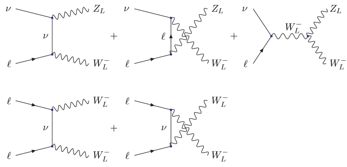
Figure 9: Feynman diagrams that contribute to the amplitude for $\ell\nu\to W^{-}_{L}Z_{L}$ and $\ell\ell\to W^{-}_{L}W^{-}_{L}$ in unitary gauge.

Appendix C

In Section 5 we considered a model for Majorana neutrino masses involving a Higgs doublet, $Y=1/2$ field, $\phi$, and a Higgs triplet, $Y=1$ field, $\Phi^{i}$. Here we discuss the scalar potential of this model.

The most general potential is [33, 34, 35, 36, 37]

$$V(\phi,\Phi^{i}) = m^{2}\phi^{\dagger}\phi+M_{T}^{2}\Phi^{i*}\Phi^{i}+\lambda_{1}(\phi^{\dagger}\phi)^{2}+\lambda_{2}(\Phi^{i*}\Phi^{i})^{2}+2\lambda_{3}(\phi^{\dagger}\phi)(\Phi^{i*}\Phi^{i})$$ (70)

$$+ \lambda_{4}(\Phi^{i}\Phi^{i})(\Phi^{j*}\Phi^{j*})-2i\lambda_{5}\epsilon^{ijk}\phi^{\dagger}\sigma^{i}\phi\Phi^{j*}\Phi^{k}$$

$$+ (M_{3}\phi^{T}\epsilon\sigma^{i}\phi\Phi^{i*}+H.c.)\;.$$

Minimizing the potential such that the neutral component of the Higgs doublet acquires a vacuum-expectation value $\langle\phi^{0}\rangle=v/\sqrt{2}$ and the neutral component of the Higgs triplet, $\Phi^{0}=(\Phi^{1}+i\Phi^{2})/\sqrt{2}$, acquires a vacuum-expectation value $\langle\Phi^{0}\rangle=u/\sqrt{2}$ yields

$$m^{2}+\lambda_{1}v^{2}+(\lambda_{3}+\lambda_{5})u^{2}-2M_{3}u=0\;,$$ (71)

$$M_{T}^{2}+\lambda_{2}u^{2}+(\lambda_{3}+\lambda_{5})v^{2}-M_{3}v^{2}/u=0\;.$$ (72)

In the limit that the mass of the Higgs-triplet field, $M_{T}$, is much greater than $v$, the equation above implies $u\approx M_{3}v^{2}/M_{T}^{2}\ll v$. Thus the small value of the vacuum-expectation value of the Higgs triplet field, $u$, can be understood as a consequence of the large value of the Higgs-triplet mass, $M_{T}$ [37].

The mass matrix of the scalar fields $\sqrt{2}{\rm Re}\,\phi^{0}$, $\sqrt{2}{\rm Re}\,\Phi^{0}$, evaluated at the minimum of the potential, is

$${\cal M}^{2}=\left(\begin{array}[]{cc}2\lambda_{1}v^{2}&2(\lambda_{3}+\lambda_{5})uv-2M_{3}v\\ 2(\lambda_{3}+\lambda_{5})uv-2M_{3}v&2\lambda_{2}u^{2}+M_{3}v^{2}/u\end{array}\right)\;.$$ (73)

The eigenvalues of this matrix are the masses of the physical scalar bosons, which must be positive. Evaluating the determinant of this matrix in the limit $M_{T}\gg v\gg u$ gives

$${\rm det}{\cal M}^{2}=2\lambda_{1}v^{2}M_{T}^{2}-4M_{3}^{2}v^{2}>0\;.$$ (74)

This equation, along with the upper bound on the Higgs self coupling, $\lambda_{1}\;{\raise 1.29167pt\hbox{$<$\kern-7.5pt\lower 4.30554pt\hbox{$\sim$}}}\;2\pi$ [10, 11], implies the bound

$$\frac{M_{3}}{M_{T}}\;{\raise 1.29167pt\hbox{$<$\kern-7.5pt\lower 4.30554pt\hbox{$\sim$}}}\;\sqrt{\pi}\;,$$ (75)

which was used in Section 5.

Appendix D

The model presented in Section 6 containing an $SU(2)_{L}$-triplet, $Y=-1$ fermion field $F_{L}^{\alpha\beta}$ and an $SU(2)_{L}$-singlet, $Y=-2$ fermion field $f_{R}^{--}$ has gauge and gravitational anomalies, and is therefore not a consistent theory. However, it is straightforward to embed this model in a theory with additional fermion fields such that it is free of all gauge and gravitational anomalies. The fermion content of this model is given in Table 3, with the right-chiral fermion fields $(F_{R}^{c})^{\alpha\beta}\equiv C\gamma^{0}F_{L}^{*\alpha\beta}$ and $f_{R}^{--}$ indicated. One can check explicitly that all anomalies cancel (including the discrete $SU(2)_{L}$ anomaly [53]).

The model was constructed as follows. One is seeking a chiral, anomaly-free $SU(3)\times SU(2)_{L}\times U(1)_{Y}$ theory containing an $SU(2)_{L}$ triplet. The smallest group with chiral, anomaly-free irreducible representations is $SO(10)$, and the smallest representation containing an $SU(2)$ triplet is the 126, which decomposes into the subgroup $SU(4)\times SU(2)\times SU(2)$ as

$$126=(6,1,1)+(\overline{10},3,1)+(10,1,3)+(15,2,2)\;.$$

The $(6,1,1)$ and $(15,2,2)$ are real representations, and hence are automatically anomaly free. The $10$ and $\overline{10}$ of $SU(4)$ decompose into the subgroup $SU(3)\times U(1)$ as

$$10 = 1(-1)+3(-1/3)+6(1/3)$$

$$\overline{10} = 1(1)+\bar{3}(1/3)+\bar{6}(-1/3)$$

and the $3$ of $SU(2)$ decomposes into the subgroup $U(1)$ as

$$3=(1)+(0)+(-1)\;.$$

Consider the decomposition $SO(10)\to SU(4)\times SU(2)\times SU(2)\to SU(3)\times SU(2)_{L}\times U(1)_{Y}$. We identify $SU(2)_{L}$ with the first $SU(2)$ and $U(1)_{Y}$ with the diagonal subgroup of the $U(1)$’s coming from the decomposition of $SU(4)$ and the second $SU(2)$ (the hypercharge is thus the sum of the two $U(1)$ charges). This yields the model in Table 3.

Table 3: $SU(3)\times SU(2)_{L}\times U(1)_{Y}$ representations of an anomaly-free model containing an $SU(2)_{L}$-triplet, $Y=1$ fermion field $(F_{R}^{c})^{\alpha\beta}$ and an $SU(2)_{L}$-singlet, $Y=-2$ fermion field $f_{R}^{--}$.

	$SU(3)$	$SU(2)_{L}$	$U(1)_{Y}$
$(F_{R}^{c})^{\alpha\beta}$	1	3	1
$f_{R}^{--}$	$1$	$1$	$-2$
	${\bar{3}}$	$3$	$1/3$
	${\bar{6}}$	$3$	$-1/3$
	$1$	$1$	$0$
	$3$	$1$	$2/3$
	$3$	$1$	$-1/3$
	$3$	$1$	$-4/3$
	$6$	$1$	$4/3$
	$6$	$1$	$1/3$
	$6$	$1$	$-2/3$

Appendix E

We derive the upper bound on the scale of Dirac-fermion mass generation, Eq. (22), in a model in which the fermion acquires a mass from the dimension-$d$ interaction of Eq. (21). The bound is obtained by applying the inelastic unitarity condition, Eq. (8) (Eq. (46) in Appendix A), to the scattering process $f_{\pm}^{Q}\bar{f}_{\pm}^{Q}\to h\cdots h$ and to the related processes in which some of the $h$’s are replaced by $Z_{L}$’s.

Begin with the dimension-$d$ interaction of Eq. (21),

$${\cal L}=-\frac{c}{M^{d-4}}{\overline{F}_{L}}^{\alpha\cdots\beta}\phi^{\alpha}\cdots\phi^{\beta}f_{R}^{Q}+H.c.\;,$$ (76)

where there are $n=d-3$ Higgs fields. Let $\phi=(-is^{+},(h+v+i\chi)/\sqrt{2})$, where $s^{+},\chi$ are the Goldstone bosons associated with $W^{+},Z$. Using the Goldstone-boson equivalence theorem, we let $\chi$ represent $Z_{L}$, and multiply by a factor of $i$ for each outgoing $Z_{L}$. The interaction of $m$ neutral Goldstone bosons with $n-m$ Higgs bosons is

$${\cal L}=-\frac{c}{M^{d-4}}\left(\frac{1}{\sqrt{2}}\right)^{n}{n\choose m}\bar{f}^{Q}\gamma_{5}^{m}f^{Q}(h)^{n-m}(i\chi)^{m}\;,$$ (77)

where $f_{L}^{Q}\equiv F_{L}^{2\cdots 2}$. The fermion acquires a mass

$$m=\frac{c}{M^{d-4}}\left(\frac{v}{\sqrt{2}}\right)^{n}\;,$$ (78)

so the Feynman rule for the $\bar{f}^{Q}f^{Q}(h)^{n-m}(\chi)^{m}$ vertex can be written as [$-i(m/v^{n})i^{m}n!\gamma_{5}^{m}$], where we have properly accounted for the $m$ identical $\chi$’s and the $n-m$ identical $h$’s.

Consider the scattering process

$$2\to n\equiv\frac{1}{\sqrt{2}}(f^{Q}_{+}\bar{f}^{Q}_{+}\mp f^{Q}_{-}\bar{f}^{Q}_{-})\to\frac{1}{\sqrt{(n-m)!}\sqrt{m!}}(h)^{n-m}(\chi)^{m}\;,$$ (79)

where the upper (lower) sign corresponds to final states with an even (odd) number of $\chi$’s. The inelastic unitarity bound, Eq. (8) (Eq. (46) in Appendix A, or, equivalently, Eq. (45)), yields

$$\left(\frac{1}{(n-1)!(n-2)!}\right)\left(\frac{1}{(2\pi)^{3}}\right)^{n}(2\pi)^{4}\frac{\pi}{2}\left(\frac{\pi}{2}s\right)^{n-2}\frac{1}{(n-m)!m!}\frac{m^{2}}{v^{2n}}2(n!)^{2}s\leq 8\pi\;,$$ (80)

where the first five factors are from $n$-body phase space. Summing over all $2\to n$ processes with $n-m$ $h$’s and $m$ $\chi$’s (with $m$ either even or odd), using

$$\sum_{m=0,2,\dots}^{n}{n\choose m}=\sum_{m=1,3,\dots}^{n}{n\choose m}=2^{n-1}\;,$$ (81)

gives

$$\left(\frac{1}{(n-1)!(n-2)!}\right)\left(\frac{1}{(2\pi)^{3}}\right)^{n}(2\pi)^{4}\frac{\pi}{2}\left(\frac{\pi}{2}s\right)^{n-2}\frac{m^{2}}{v^{2n}}2n!2^{n-1}s\leq 8\pi\;.$$ (82)

Defining $\Lambda_{d}$ as the energy, $\sqrt{s}$, at which this inequality is saturated yields Eq. (22),

$$\Lambda_{d}\equiv 4\pi\kappa_{d}\left(\frac{v^{d-3}}{m_{f}}\right)^{1/(d-4)}\;,$$ (83)

where we have used $n=d-3$ and

$$\kappa_{d}\equiv\left(\sqrt{\frac{(d-5)!}{2^{d-5}(d-3)}}\right)^{1/(d-4)}\;.$$ (84)

Appendix F

In Refs. [4, 5] a two-Higgs-doublet model was studied in the limit that the mass of the Higgs scalar $H$ is large and one or more quartic couplings grows with the mass of this Higgs scalar. The limits studied in those papers appear to be the same. Here we show that they are actually different limits. Nevertheless, they are both unphysical because they require a dimensionless coupling to exceed ${\cal O}(4\pi)$.

The Higgs potential used in Ref. [4] is given in Eq. (30). In Ref. [5], a different but physically equivalent parameterization of the Higgs potential is used [55]:

$$V(\phi_{1},\phi_{2}) = \lambda_{1}^{\prime}(\phi_{1}^{\dagger}\phi_{1}-v_{1}^{2}/2)^{2}+\lambda_{2}^{\prime}(\phi_{2}^{\dagger}\phi_{2}-v_{2}^{2}/2)^{2}$$ (85)

$$+ \lambda_{3}^{\prime}[(\phi_{1}^{\dagger}\phi_{1}-v_{1}^{2}/2)+(\phi_{2}^{\dagger}\phi_{2}-v_{2}^{2}/2)]^{2}+\lambda_{4}^{\prime}[(\phi_{1}^{\dagger}\phi_{1})(\phi_{2}^{\dagger}\phi_{2})-(\phi_{1}^{\dagger}\phi_{2})(\phi_{2}^{\dagger}\phi_{1})]$$

$$+ \lambda_{5}^{\prime}[{\rm Re}\,(\phi_{1}^{\dagger}\phi_{2})-v_{1}v_{2}/2]^{2}+\lambda_{6}^{\prime}[{\rm Im}\,(\phi_{1}^{\dagger}\phi_{2})]^{2}\;.$$

The coefficients are labeled $\lambda_{i}^{\prime}$ to distinguish them from the coefficients $\lambda_{i}$ in Eq. (30). They are related to the parameters of the Higgs potential given in Eq. (30) by

$$\lambda_{1} = 2(\lambda_{1}^{\prime}+\lambda_{3}^{\prime})$$

$$\lambda_{2} = 2(\lambda_{2}^{\prime}+\lambda_{3}^{\prime})$$

$$\lambda_{3} = 2\lambda_{3}^{\prime}+\lambda_{4}^{\prime}$$

$$\lambda_{4} = \frac{1}{2}(\lambda_{5}^{\prime}+\lambda_{6}^{\prime})-\lambda_{4}^{\prime}$$

$$\lambda_{5} = \frac{1}{2}(\lambda_{5}^{\prime}-\lambda_{6}^{\prime})$$

$$m_{11}^{2} = -v_{1}^{2}(\lambda_{1}^{\prime}+\lambda_{3}^{\prime})-v_{2}^{2}\lambda_{3}^{\prime}$$

$$m_{22}^{2} = -v_{2}^{2}(\lambda_{2}^{\prime}+\lambda_{3}^{\prime})-v_{1}^{2}\lambda_{3}^{\prime}$$

$$m_{12}^{2} = \frac{1}{2}v_{1}v_{2}\lambda_{5}^{\prime}$$

The limit studied in Ref. [5] corresponds to taking $m_{H}$ large by letting $\lambda_{5}^{\prime}\to\infty$ , since they are approximately related by

$$m_{H}^{2}\approx\frac{1}{2}\lambda_{5}^{\prime}v^{2}\;,$$ (86)

where $v=(\sqrt{2}G_{F})^{-1/2}$ is the weak scale. In terms of the parameterization of Eq. (30), used in Ref. [4], this limit corresponds to $\lambda_{4}=\lambda_{5}=m_{12}^{2}/v_{1}v_{2}\to\infty$, as is evident from the above relations. This differs from the limit studied in Ref. [4], which corresponds to $\lambda_{5}\to\infty$, with $\lambda_{5}\sin^{2}\beta$ and $m_{12}^{2}\sin\beta$ fixed. In terms of the parameterization of Eq. (85), used in Ref. [5], this limit corresponds to $\lambda_{5}^{\prime}=-\lambda_{6}^{\prime}\to\infty$, with $\lambda_{5}^{\prime}\sin^{2}\beta$ fixed.

References

- [1] M. S. Chanowitz and M. K. Gaillard, Nucl. Phys. B261, 379 (1985).
- [2] T. Appelquist and M. S. Chanowitz, Phys. Rev. Lett. 59, 2405 (1987).
- [3] M. Golden, Phys. Lett. B338, 295 (1994) [hep-ph/9408272].
- [4] S. Jager and S. Willenbrock, Phys. Lett. B435, 139 (1998) [hep-ph/9806286].
- [5] R. S. Chivukula, Phys. Lett. B439, 389 (1998) [hep-ph/9807406].
- [6] F. Maltoni, J. M. Niczyporuk and S. Willenbrock, Phys. Rev. Lett. 86, 212 (2001) [hep-ph/0006358].
- [7] C. G. Callan, S. Coleman, J. Wess and B. Zumino, Phys. Rev. 177, 2247 (1969).
- [8] T. Appelquist and C. Bernard, Phys. Rev. D 22, 200 (1980).
- [9] W. Marciano, G. Valencia and S. Willenbrock, Phys. Rev. D 40, 1725 (1989).
- [10] R. Dashen and H. Neuberger, Phys. Rev. Lett. 50, 1897 (1983).
- [11] M. Luscher and P. Weisz, Phys. Lett. B212, 472 (1988).
- [12] T. Appelquist and J. Carazzone, Phys. Rev. D 11, 2856 (1975).
- [13] J. M. Cornwall, D. N. Levin and G. Tiktopoulos, Phys. Rev. Lett. 30, 1268 (1973).
- [14] J. M. Cornwall, D. N. Levin and G. Tiktopoulos, Phys. Rev. D 10, 1145 (1974).
- [15] C. H. Llewellyn Smith, Phys. Lett. B46, 233 (1973).
- [16] C. E. Vayonakis, Lett. Nuovo Cim. 17, 383 (1976).
- [17] B. W. Lee, C. Quigg and H. B. Thacker, Phys. Rev. D 16, 1519 (1977).
- [18] J. Bagger and C. Schmidt, Phys. Rev. D 41, 264 (1990).
- [19] L. Maiani, G. Parisi and R. Petronzio, Nucl. Phys. B 136, 115 (1978).
- [20] N. Cabibbo, L. Maiani, G. Parisi and R. Petronzio, Nucl. Phys. B158, 295 (1979).
- [21] B. Pendleton and G. G. Ross, Phys. Lett. B 98, 291 (1981).
- [22] W. A. Bardeen, C. T. Hill and M. Lindner, Phys. Rev. D 41, 1647 (1990).
- [23] H. Georgi, Nucl. Phys. B 156, 126 (1979).
- [24] S. Weinberg, Phys. Rev. Lett. 43, 1566 (1979).
- [25] A. Aguilar et al. [LSND Collaboration], hep-ex/0104049.
- [26] T. Toshito [SuperKamiokande Collaboration], hep-ex/0105023.
- [27] J. N. Bahcall, P. I. Krastev and A. Y. Smirnov, JHEP 0105, 015 (2001) [hep-ph/0103179].
- [28] M. Gell-Mann, P. Ramond, and R. Slansky, in Supergravity, eds. P. van Nieuwenhuizen and D. Freedman (North Holland, Amsterdam, 1979), p. 315; T. Yanagida, in Proceedings of the Workshop on Unified Theory and Baryon Number in the Universe, eds. O. Sawada and A. Sugamoto (KEK, Tsukuba, Japan, 1979).
- [29] R. N. Mohapatra and G. Senjanovic, Phys. Rev. Lett. 44, 912 (1980).
- [30] M. S. Chanowitz, M. A. Furman and I. Hinchliffe, Nucl. Phys. B153, 402 (1979).
- [31] M. B. Einhorn and G. J. Goldberg, Phys. Rev. Lett. 57, 2115 (1986).
- [32] I. Lee, J. Shigemitsu and R. E. Shrock, Nucl. Phys. B 330, 225 (1990).
- [33] T. P. Cheng and L. Li, Phys. Rev. D 22, 2860 (1980).
- [34] G. B. Gelmini and M. Roncadelli, Phys. Lett. B99, 411 (1981).
- [35] R. N. Mohapatra and G. Senjanovic, Phys. Rev. D 23, 165 (1981).
- [36] H. M. Georgi, S. L. Glashow and S. Nussinov, Nucl. Phys. B193, 297 (1981).
- [37] E. Ma and U. Sarkar, Phys. Rev. Lett. 80, 5716 (1998) [hep-ph/9802445].
- [38] W. Buchmuller and D. Wyler, Nucl. Phys. B 268, 621 (1986).
- [39] H. E. Haber, in Proceedings of the Workshop on Perspectives for Electroweak Interactions in Collisions, Ringberg Castle, Germany, February 5–8, ed. B. Kniehl (World Scientific, Singapore, 1995), p. 219, hep-ph/9505240.
- [40] G. P. Lepage and S. J. Brodsky, Phys. Rev. D 22, 2157 (1980).
- [41] S. Weinberg, Phys. Rev. D 19, 1277 (1979).
- [42] L. Susskind, Phys. Rev. D 20, 2619 (1979).
- [43] E. Eichten and K. Lane, Phys. Lett. B 90, 125 (1980).
- [44] S. Dimopoulos and L. Susskind, Nucl. Phys. B 155, 237 (1979).
- [45] B. Holdom, Phys. Rev. D 24, 1441 (1981).
- [46] B. Holdom, Phys. Lett. B 150, 301 (1985).
- [47] K. Yamawaki, M. Bando and K. Matumoto, Phys. Rev. Lett. 56, 1335 (1986).
- [48] T. W. Appelquist, D. Karabali and L. C. Wijewardhana, Phys. Rev. Lett. 57, 957 (1986).
- [49] T. Appelquist, M. Einhorn, T. Takeuchi and L. C. Wijewardhana, Phys. Lett. B 220, 223 (1989).
- [50] T. Takeuchi, Phys. Rev. D 40, 2697 (1989).
- [51] V. A. Miransky and K. Yamawaki, Mod. Phys. Lett. A 4, 129 (1989).
- [52] R. S. Chivukula, A. G. Cohen and K. Lane, Nucl. Phys. B 343, 554 (1990).
- [53] E. Witten, Phys. Lett. B117, 324 (1982).
- [54] R. Slansky, Phys. Rept. 79, 1 (1981).
- [55] H. Georgi, Hadronic J. 1, 155 (1978).