hep-ph/0106280

FERMILAB-Pub-01/190-T

Predictions of the sign of $\mu$ from supersymmetry breaking models

Stephen P. Martin

Department of Physics, Northern Illinois University, DeKalb IL 60115 $\rm and$
Fermi National Accelerator Laboratory, P.O. Box 500, Batavia IL 60510

The sign of the supersymmetric Higgs mass $\mu$ is usually taken as an independent input parameter in analyses of the supersymmetric standard model. I study the role of theories of supersymmetry breaking in determining the sign of $\mu$ as an output. Models with vanishing soft scalar couplings at the apparent gauge coupling unification scale are known to predict positive $\mu$. I investigate more general results for the sign of $\mu$ as a function of the holomorphic soft scalar couplings, and compare to predictions of models with gaugino mass dominance at higher scales. In a significant region of the $B_{0}/m_{1/2}$ versus $A_{0}/m_{1/2}$ plane including $A_{0}=B_{0}=0$, $\mu$ must be positive. In another region, $\mu$ is definitely negative. Only in a smaller intermediate region does knowledge of the supersymmetry breaking mechanism not permit a definite prediction of the sign of $\mu$. The last region will shrink considerably as the top quark mass becomes more accurately known.

In the minimal supersymmetric standard model (MSSM) [1, 2], the Higgs mass term $\mu$ is the only coupling which does not explicitly break supersymmetry that has not already been directly measured by experiment. Nevertheless, in phenomenological treatments of supersymmetric models, it is usual to treat $|\mu|$ as an output rather than an input parameter, because it can be fixed in terms of the other parameters from our knowledge of the electroweak scale. However, this condition alone does not address the phase of $\mu$, which is left unfixed by the conditions of electroweak symmetry breaking (EWSB). The lack of observed CP violation in the electric dipole moments of the neutron and electron requires that large relative phases in the MSSM lagrangian must either be absent or aligned to rather particular values. Barring the latter possibility, it follows that all gaugino masses should be (at least nearly) relatively real, and that with appropriately chosen phase conventions $\mu$ is real and the phases of scalar cubic couplings are equal to their Yukawa coupling counterparts.

The remaining discrete phase freedom sign$(\mu)$ is therefore usually regarded as an independent input parameter. However, if the mechanism of supersymmetry breaking is known, the phase of $\mu$ including its sign is often determined purely from the theory and knowledge of already-measured dimensionless supersymmetry-preserving couplings. This has been noted before in the contexts of flipped $SU(5)\times U(1)$ no-scale supergravity models [4] and in gauge-mediated supersymmetry breaking models[13]-[16]. More generally, a complete model of supersymmetry breaking should predict boundary conditions for all soft parameters in terms of supersymmetric parameters. This implies that, under many (but not all!) circumstances, the sign of $\mu$ should properly be regarded as an output prediction rather than an input assumption. Conversely, an experimental determination of the sign of $\mu$ will provide a non-trivial test of different models of supersymmetry breaking. In this paper I will study the ability of flavor-preserving high-scale theories of supersymmetry breaking to predict the sign of $\mu$, and consider under what circumstances such a prediction can be made unambiguously.

In this paper, it is assumed that the gaugino mass parameters $M_{1}$, $M_{2}$, and $M_{3}$ indeed have the same phase, so that they can be taken real and positive without loss of generality. To fix conventions explicitly, the tree-level neutral Higgs potential is given by

$$V\! = \!(|\mu|^{2}+m^{2}_{H_{u}})|H_{u}^{0}|^{2}+(|\mu|^{2}+m^{2}_{H_{d}})|H_{d}^{0}|^{2}-(b\,H_{u}^{0}H_{d}^{0}+{\rm c.c.})$$ (1)

$$+{1\over 8}(g^{2}+g^{\prime 2})(|H_{u}^{0}|^{2}-|H_{d}^{0}|^{2})^{2},$$

Here $b$ is the holomorphic soft supersymmetry-breaking Higgs squared mass parameter. (Other common notations in the literature for this term are $B\mu$ and $m_{12}^{2}$ and $m_{3}^{2}$.) Without loss of generality, a suitably renormalized $b$ is taken to be real and positive at a renormalization group (RG) scale near or below 1 TeV, to fulfill the condition that at the minimum of the effective potential, the Higgs fields will have real positive VEVs:

$$\langle H_{u}^{0}\rangle=v_{u};\qquad\langle H_{d}^{0}\rangle=v_{d};\qquad v_{u}^{2}+v_{d}^{2}\approx(175\>{\rm GeV})^{2};\qquad v_{u}/v_{d}\equiv\tan\beta.$$ (2)

The tree-level top, bottom and tau masses and Yukawa couplings $m_{t}=v_{u}y_{t}$, $m_{b}=v_{d}y_{b}$ and $m_{\tau}=v_{d}y_{\tau}$ are simultaneously real and positive. (Lighter fermion masses are neglected, so CKM CP violation is not an issue.) Neutralino and chargino mass matrices are given by

$${\bf M}_{\widetilde{N}}=\pmatrix{M_{1}&0&-g^{\prime}v_{d}/\sqrt{2}&g^{\prime}v_{u}/\sqrt{2}\cr 0&M_{2}&gv_{d}/\sqrt{2}&-gv_{u}/\sqrt{2}\cr-g^{\prime}v_{d}/\sqrt{2}&gv_{d}/\sqrt{2}&0&-\mu\cr g^{\prime}v_{u}/\sqrt{2}&-gv_{u}/\sqrt{2}&-\mu&0},\qquad{\bf M}_{\widetilde{C}}=\pmatrix{M_{2}&gv_{u}\cr gv_{d}&\mu}.$$ (3)

The relevant soft supersymmetry-breaking terms include

$$-{\cal L}_{\rm soft} = -bH_{u}^{0}H_{d}^{0}+a_{t}\widetilde{t}_{L}\widetilde{t}_{R}^{*}H_{u}^{0}+a_{b}\widetilde{b}_{L}\widetilde{b}^{*}_{R}H_{d}^{0}+a_{\tau}\widetilde{\tau}_{L}\widetilde{\tau}_{R}^{*}H_{d}^{0}+{\rm c.c.},$$ (4)

so that the stop and sbottom squared mass matrices are:

$${\bf m}^{2}_{\widetilde{t}} = \pmatrix{m^{2}_{\widetilde{t}_{L}}+y_{t}^{2}v_{u}^{2}+D_{\widetilde{t}_{L}}&a_{t}v_{u}-\mu y_{t}v_{d}\cr a_{t}v_{u}-\mu y_{t}v_{d}&m^{2}_{\widetilde{t}_{R}}+y_{t}^{2}v_{u}^{2}+D_{\widetilde{t}_{R}}};$$ (5)

$${\bf m}^{2}_{\widetilde{b}} = \pmatrix{m^{2}_{\widetilde{b}_{L}}+y_{b}^{2}v_{d}^{2}+D_{\widetilde{b}_{L}}&a_{b}v_{d}-\mu y_{b}v_{u}\cr a_{b}v_{d}-\mu y_{b}v_{u}&m^{2}_{\widetilde{b}_{R}}+y_{b}^{2}v_{d}^{2}+D_{\widetilde{b}_{R}}},$$ (6)

where $D_{\phi}=(g^{2}T^{\phi}_{3}-g^{\prime 2}Y^{\phi})(v_{d}^{2}-v_{u}^{2})/2$. These phase conventions agree with those in [1, 2].

Within the framework of supersymmetry breaking communicated by arbitrary Planck-suppressed operators, the assumption that $\mu$ is real is a strong and seemingly unnatural one, requiring justification in terms of some organizing principle. One way of addressing this is to require that gaugino masses are the dominant source of all supersymmetry breaking at some RG input scale $M_{\rm X}$. Other soft supersymmetry-breaking parameters can then be thought of as radiative effects due to large logarithms which can be resummed using the renormalization group. Older versions of this idea followed from the ideas of “no-scale” supergravity models [3, 4], and it has found a different justification recently in terms of models with supersymmetry breaking displaced along compactified extra dimensions [5]-[11]. A crucial benefit of these models is that they naturally avoid the most dangerous types of supersymmetric flavor violation, since the gaugino interactions which communicate supersymmetry breaking to the sfermion masses are automatically flavor-blind.

If gaugino masses have a common phase and are the dominant source of supersymmetry breaking, then it is well-known that $\mu$ can be taken to be real without loss of generality. One way to understand this is to consider the form of the RG equations for the holomorphic scalar supersymmetry-breaking interactions $b$, $a_{t}$, $a_{b}$, and $a_{\tau}$. At all orders in perturbation theory, these can be written in the form[12]:

$${d\over dt}(a_{f}/y_{f}) = -2{\cal O}[\beta(y_{f})/y_{f}],$$ (7)

$${d\over dt}(b/\mu) = -2{\cal O}[\beta(\mu)/\mu]$$ (8)

where

$${\cal O} \equiv {1\over 2}\sum_{a}M_{a}g_{a}{\partial\over\partial g_{a}}-\sum_{f}a_{f}{\partial\over\partial y_{f}}$$ (9)

is a differential operator on the space of gauge and holomorphic couplings. The index $a$ labels the gauge groups with gauge couplings $g_{a}$ and gaugino masses $M_{a}$, and $t={\rm ln}(Q/Q_{0})$ with $Q$ the RG scale. If $b/\mu$, $a_{t}/y_{t}$, $a_{b}/y_{b}$, and $a_{\tau}/y_{\tau}$ are negligible at the input scale and are generated by radiative corrections, they will be real at all other scales, since $\cal O$ is linear in $M_{a}$ and $a_{f}$ and the quantities $\beta(y_{f})/y_{f}$ and $\beta(\mu)/\mu$ are sums of real superfield anomalous dimensions. Since $b$, $y_{t}$, $y_{b}$, $y_{\tau}$, and one $M_{a}$ are real by convention, and the other $M_{a}$ are real by assumption, it follows that $\mu$, $a_{t}$, $a_{b}$, $a_{\tau}$ are real within the same set of conventions.

The fact that the running gauge couplings of the MSSM are found to nearly meet at a scale near $2\times 10^{16}$ GeV is suggestive that a perturbative RG analysis can be applied for all couplings and parameters up to that scale. However, whether in models of extra dimensions, or “no-scale” models, or supergravity-inspired models which happen to have gaugino mass domination, it is likely that the true input scale is higher, perhaps at the reduced Planck scale $M_{\rm P}=2.4\times 10^{18}$ GeV. It is difficult to say with any confidence what the RG running should be like above $M_{\rm U}$, except that the evolution of soft parameters is significant and dominated by gaugino mass effects. Therefore, it is useful to work with boundary conditions for the gaugino masses $M_{1}$, $M_{2}$, $M_{3}$ and soft scalar interactions:

$$b/\mu\equiv B_{0}$$ (10)

$$a_{t}/y_{t}=A_{0t};\qquad a_{b}/y_{b}=A_{0b};\qquad a_{\tau}/y_{\tau}=A_{0\tau}$$ (11)

imposed at $M_{\rm U}\equiv 2\times 10^{16}$ GeV (except as noted below). If gaugino mass domination is input at $M_{\rm U}$, then one would have $A_{0t}=A_{0b}=A_{0\tau}=B_{0}=0$ at that scale. However, if the true input scale is higher, then an examination of the perturbative form of the beta functions eqs. (7)-(9) shows that $B_{0}$ and $A_{0t}$, $A_{0b}$, $A_{0\tau}$ will each be negative at $M_{\rm U}$ due to loops involving gauginos.

In general one expects that $A_{0t}$, $A_{0b}$, $A_{0\tau}$ obtain different corrections from physics above $M_{\rm U}$, depending on how the MSSM superfields fit into whatever gauge group may reign in that regime. Similarly, the non-holomorphic scalar squared masses will not be universal at $M_{\rm U}$ if they occupy different representations of the gauge group. In a study of the sparticle spectrum, it would be crucial to assume knowledge of these particulars. However, the results below regarding the sign of $\mu$ depend only weakly on the effects of non-universal non-holomorphic scalar masses, which do not enter directly in the RG equations that can affect the running of the crucial quantity $b/\mu$. Also, the dependence of the running of $b/\mu$ on scalar cubic couplings below $M_{\rm U}$ is mostly due (at least at small or moderate $\tan\beta$) to the single quantity $A_{0t}$, which in many models is not very different from $A_{0b}$ anyway. Results for the case that the gaugino masses do not unify at $M_{\rm U}$ are beyond the scope of this paper, but I expect them to behave in a similar way to the results below as long as the ratios among $M_{1}$, $M_{2}$ and $M_{2}$ are moderate. Therefore, for concreteness and simplicity I will use the traditional boundary conditions

$$m_{1/2} = M_{1}=M_{2}=M_{3};$$ (12)

$$A_{0} = A_{0t}=A_{0b}=A_{0\tau};$$ (13)

$$m_{0}^{2} = m_{\phi}^{2}\qquad({\rm for}\>{\rm all}\>{\rm\phi})$$ (14)

as a convenient parameterization of our ignorance regarding the true boundary conditions at $M_{\rm U}$. Each model is then characterized by an overall gaugino mass scale $m_{1/2}$ and ratios $B_{0}/m_{1/2}$, $A_{0}/m_{1/2}$, and $m^{2}_{0}/m^{2}_{1/2}$. In gaugino mass dominated models, one generally expects the effective $B_{0}/m_{1/2}$, $A_{0}/m_{1/2}$ at $M_{\rm U}$ to be negative and not too large in magnitude.

In practice, the relation between the sign of $\mu$ and the high-scale boundary conditions is accomplished by choosing $\mu$ and $b$ near the electroweak scale to produce correct EWSB, running them up to $M_{\rm U}$, and then iterating to the desired boundary conditions. I use 2-loop RG equations [17, 18] for all MSSM parameters. The conversion of Standard Model $\overline{{\rm MS}}$ quantities to MSSM $\overline{{\rm DR}}^{\prime}$ [19, 18] ones, and the relation between pole masses and running parameters is accomplished using ref. [20]. The conditions for EWSB, the values of $v_{u}$ and $v_{d}$, and the physical masses of Higgs scalar bosons are calculated using the full one-loop self-energy corrections plus the leading two-loop effective potential corrections, namely those proportional to $g_{3}^{2}$ [21] and those quartic in $y_{t}$ and $y_{b}$ [22]. The effective potential minimization is performed at an RG scale equal to the geometric mean of the stop masses. In this paper, values of $\tan\beta$ are always quoted as the ratio of running VEVs at $M_{Z}$ in the non-decoupling $\overline{\rm DR}^{\prime}$ scheme in Landau gauge, determined by running according to the one-loop RG equations[23]

$${d\over dt}{\rm ln}(v_{u}) = {1\over 16\pi^{2}}\left[-3y_{t}^{2}+{3\over 4}g_{2}^{2}+{3\over 20}g_{1}^{2}\right];$$ (15)

$${d\over dt}{\rm ln}(v_{d}) = {1\over 16\pi^{2}}\left[-3y_{b}^{2}-y_{\tau}^{2}+{3\over 4}g_{2}^{2}+{3\over 20}g_{1}^{2}\right]$$ (16)

from the scale at which the effective potential is minimized. The largest uncertainties in the following come from not knowing the precise values of the top and bottom quark masses and the QCD coupling. I take central values and allowed ranges as follows:

$$\alpha_{3}^{\overline{\rm MS}}(M_{Z}) = 0.118\pm 0.003;$$ (17)

$$m_{b}^{\overline{\rm MS}}(M_{Z}) = 2.88+16(0.118-\alpha_{3})\pm 0.10\>{\rm GeV};$$ (18)

$$m_{t}^{\rm pole} = 174.3\pm 8.0\>{\rm GeV}.$$ (19)

Here $\alpha_{3}^{\overline{\rm MS}}$ and $m_{b}^{\overline{\rm MS}}$ are running parameters in the Standard Model with 5 quark flavors. The range in the top quark mass is larger than that quoted in [24], because of the theoretical uncertainty in relating the top-quark Yukawa coupling to the pole mass in supersymmetry.

The RG evolution of the dimensionless ratio $b/\mu m_{1/2}$ is given in fig. 1(a) for an example gaugino-mass-dominated model with $A_{0}=B_{0}=0$ at $M_{\rm X}=M_{\rm U}$.

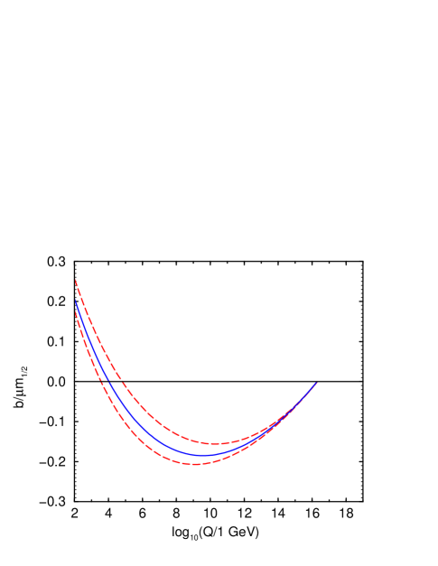
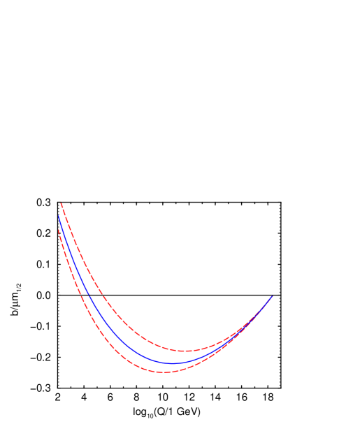
Figure 1: Running of the dimensionless ratio of parameters $b/\mu m_{1/2}$ with the boundary conditions $A_{0}=B_{0}=m_{0}=0$ and $m_{1/2}=400$ GeV imposed at (a) $M_{\rm U}=2\times 10^{16}$ GeV and (b) $M_{\rm P}=2.4\times 10^{18}$ GeV. The solid (blue) lines are obtained for the central values, and the dashed (red) lines for the maximum deviation, implied by eqs. (17)-(19). Since $b/\mu m_{1/2}$ is positive at the weak scale, $\mu$ must be positive.

(The graphs shown also use $m_{1/2}=400$ GeV, and $m^{2}_{0}=0$, but they depend only weakly on those choices.) With these boundary conditions, $\tan\beta$ is uniquely determined by the requirements of correct electroweak symmetry breaking, so there is only one possible RG trajectory for the parameters of the model once $\alpha_{3}$, $m_{b}$ and $m_{t}$ are fixed.. As shown, $b/\mu m_{1/2}$ is negative along most of its evolution towards the infrared, but turns positive at a scale about two or three orders of magnitude above the electroweak scale. This can be explained as follows. The one-loop RG equations for the holomorphic soft couplings following from eq. (7)-(8) are:

$$16\pi^{2}{d\over dt}(a_{t}/y_{t}) = {32\over 3}g_{3}^{2}M_{3}+6g_{2}^{2}M_{2}+{26\over 15}g_{1}^{2}M_{1}+12a_{t}y_{t}+2a_{b}y_{b};$$ (20)

$$16\pi^{2}{d\over dt}(a_{b}/y_{b}) = {32\over 3}g_{3}^{2}M_{3}+6g_{2}^{2}M_{2}+{14\over 15}g_{1}^{2}M_{1}+12a_{b}y_{b}+2a_{t}y_{t}+2a_{\tau}y_{\tau};$$ (21)

$$16\pi^{2}{d\over dt}(a_{\tau}/y_{\tau}) = 6g_{2}^{2}M_{2}+{18\over 5}g_{1}^{2}M_{1}+8a_{\tau}y_{\tau}+6a_{b}y_{b};$$ (22)

$$16\pi^{2}{d\over dt}(b/\mu) = 6g_{2}^{2}M_{2}+{6\over 5}g_{1}^{2}M_{1}+6a_{t}y_{t}+6a_{b}y_{b}+2a_{\tau}y_{\tau}.$$ (23)

At high RG scales, gaugino masses are dominant, quickly driving each of $a_{f}/y_{f}$ and $b/\mu$ to negative values in the infrared. Continuing to lower RG scales, the dominant contributions to the beta function for $b/\mu$ are the negative ones proportional to $a_{t}y_{t}$, $a_{b}y_{b}$ and $a_{\tau}y_{\tau}$. This forces $b/\mu$ positive before the electroweak scale is reached. There is a significant dependence on the top mass and a smaller dependence on the bottom mass and $\alpha_{3}$, shown by the envelope of dashed lines. Since $b$ is positive near the electroweak scale by convention, the sign of $\mu$ is the same as the sign of the dimensionless quantity $b/\mu m_{1/2}$. Because there is a unique solution for $\tan\beta$, the conclusion is that $\mu$ is inevitably positive.

The model shown in fig. 1(a) predicts $\tan\beta$ should be between about 10 (for larger $m_{\rm top}$, corresponding to the upper dashed line) and 24 (for smaller $m_{\rm top}$, corresponding to the lower dashed line). It also generally predicts that a stau is the lightest supersymmetric particle (LSP), abandoning the possibility of a supersymmetric source for the cold dark matter. This is easily corrected if the true input scale is higher than $M_{\rm U}$. An example of this is shown in fig. 1(b), for which the scale at which the boundary conditions eq. (10)-(14) with $m_{0}=A_{0}=B_{0}=0$ are moved up to the reduced Planck scale $M_{\rm P}$. For simplicity, no new particle thresholds are introduced at the apparent unification scale. As before, the running of $b/\mu$ renders it positive at the electroweak scale, implying again that $\mu$ must be positive. In this ultraconservative version of the MSSM with no new particles and gaugino mass domination at the Planck scale, a bino-like neutralino is the LSP.

More generally, for given RG trajectories of the dimensionless supersymmetric parameters, the running of the dimensionless quantity $b/\mu m_{1/2}$ is determined uniquely by its boundary condition $B_{0}/m_{1/2}$ and that of the scalar cubic couplings, $A_{0}/m_{1/2}$ at $M_{\rm U}$. This can be checked from the form of eqs. (7), (8). The effect on the sign of $\mu$ can be roughly stated as follows. Lowering $A_{0}/m_{1/2}$ tends to make the beta function for $b/\mu$ more negative, making $b/\mu m_{1/2}$ more positive at the weak scale, thus increasing the parameter space in other variables for which $\mu$ must be positive. Lowering $B_{0}/m_{1/2}$ will have the opposite effect, since for very negative $B_{0}$, only negative $\mu$ can rescue $b/\mu$ to make it positive near the electroweak scale. Therefore, one can map out regions of the $B_{0}/m_{1/2}$ versus $A_{0}/m_{1/2}$ which predict that $\mu$ is definitely positive, definitely negative, or can have either sign.

Figure 2 shows the region for which $\mu$ can be positive, for

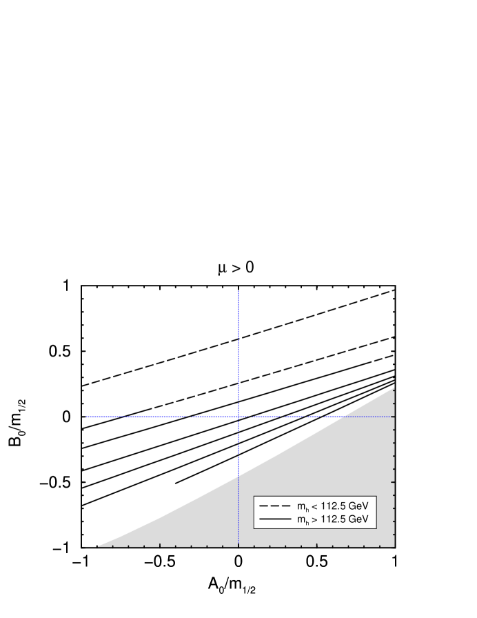
Figure 2: The region of the $B_{0}/m_{1/2}$ vs. $A_{0}/m_{1/2}$ plane which allows $\mu>0$ is unshaded. Boundary conditions are imposed at $M_{\rm U}=2\times 10^{16}$ GeV, with gaugino masses restricted by $m_{1/2}<400$ GeV and scalar masses in the range $0<m_{0}^{2}/m_{1/2}^{2}<1$. All values of $\tan\beta$ leading to correct EWSB, perturbative couplings up to $M_{U}$, and charged superpartners heavier than 100 GeV are allowed. Example models lines are shown for $\tan\beta=3,6,10,20,30,40,50$ (from top to bottom), with $m_{1/2}=350$ GeV, $m_{0}^{2}/m_{1/2}^{2}=0.5$.

$m_{1/2}<400$ GeV and $0<m_{0}^{2}/m_{1/2}^{2}<1$. In making this graph, all values of $\tan\beta$ which maintain perturbative couplings up to $M_{\rm U}$ are allowed, and the top and bottom quark masses and $\alpha_{3}$ are allowed to vary over the full ranges indicated in eq. (17)-(19). All charged sparticle masses are required to be heavier than 100 GeV. The shaded region indicates where no solution with $\mu>0$ can be found. Smaller values of $\tan\beta$ corresponds to points with larger $B_{0}/m_{1/2}$, while the largest allowed $\tan\beta$ values occur near the boundary of the unshaded region. Several example model lines with fixed $\tan\beta=3,6,10,20,30,40,50$ are also shown; these were computed with $m_{1/2}=350$ GeV, $m_{0}^{2}/m_{1/2}^{2}=0.5$ and central values for the top and bottom masses and $\alpha_{3}$. I have also indicated by dashed lines those models for which the lightest CP-even Higgs mass $m_{h}$ calculated as indicated above comes out lighter than 112.5 GeV, for rough comparison with LEP2 limits. (Even with full one-loop and leading two-loop calculations, it can be estimated from scale-dependence considerations that there is at least a 2 GeV uncertainty in the calculated $m_{h}$.)

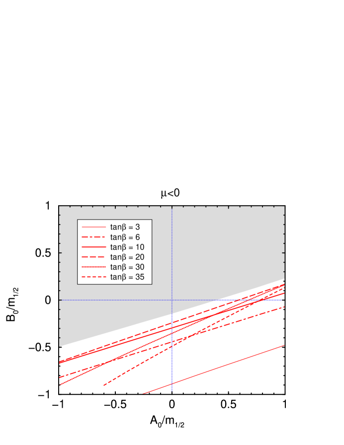
Figure 3: The region of the $B_{0}/m_{1/2}$ vs. $A_{0}/m_{1/2}$ plane which allows $\mu<0$ is unshaded. Universal gaugino masses are restricted by $m_{1/2}<400$ GeV and universal scalar masses lie in the range $0<m_{0}^{2}/m_{1/2}^{2}<1$. All values of $\tan\beta$ leading to correct EWSB, perturbative couplings up to $M_{U}$, and charged superpartners heavier than 100 GeV are allowed. Example model lines are shown for various values of $\tan\beta$, using $m_{1/2}=350$ GeV, $m_{0}^{2}/m_{1/2}^{2}=0.5$.

In contrast, fig. 3 shows the region which allows negative $\mu$ under the same assumptions. As suggested by fig. 1(a), there is a significant neighborhood of the point $A_{0}/m_{1/2}=B_{0}/m_{1/2}=0$ which cannot support negative $\mu$. Here, this is shown to be true for any values of $m_{1/2}<400$ GeV and $0<m^{2}_{0}/m_{1/2}^{2}<1$ and with top and bottom quark masses and $\alpha_{3}$ allowed to vary over the entire ranges indicated in eq. (17)-(19). Models which approach the border of the allowed region with $\mu<0$ turn out to have intermediate values of $\tan\beta$ (typically between 10 and 25), while smaller or larger $\tan\beta$ models have larger negative $B_{0}/m_{1/2}$.

The regions in figs. 2 and 3 allowed for positive and negative $\mu$ have a significant overlap. This represents a true ambiguity in the sign of $\mu$, even in models for which the boundary conditions for the soft supersymmetry breaking couplings are fully specified, and even if the QCD coupling and physical top and bottom masses were known with arbitrary accuracy. To illustrate this, fig. 4 shows solutions for $\tan\beta$ as a function of a single varying parameter $B_{0}/m_{1/2}$, with fixed $A_{0}=-0.75m_{1/2}$, $m_{1/2}=400$ GeV and $m_{0}^{2}/m_{1/2}^{2}=0.5$ and $\alpha_{3}$, $m_{b}$ and $m_{t}$ taking there central values..

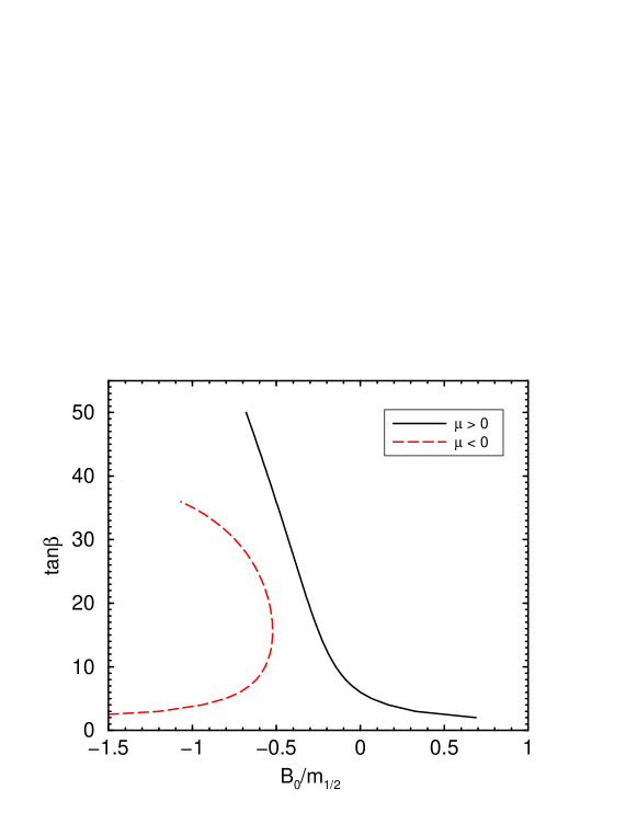
Figure 4: Solutions for $\tan\beta$ as a function of $B_{0}/m_{1/2}$, for $\mu>0$ (solid black) and $\mu<0$ (dashed red). In each case, the boundary conditions imposed at $M_{\rm U}=2\times 10^{16}$ GeV are $A_{0}=-0.75m_{1/2}$, with $m_{1/2}=400$ GeV and $m_{0}^{2}/m_{1/2}^{2}=0.5$. This illustrates that for a range of $B_{0}/m_{1/2}$ (here, $-0.7$ to $-0.5$), there are sometimes simultaneously distinct solutions with positive $\mu$ and negative $\mu$. For larger $B_{0}/m_{1/2}$, $\mu$ is definitely positive, while for smaller $B_{0}/m_{1/2}$, $\mu$ is definitely negative.

For $B_{0}/m_{1/2}\lower 3.01385pt\hbox{$\;\stackrel{{\scriptstyle\textstyle>}}{{\sim}}\;$}-0.5$, there is always only one solution for $\tan\beta$, corresponding to positive $\mu$. For $B_{0}/m_{1/2}\lower 3.01385pt\hbox{$\;\stackrel{{\scriptstyle\textstyle<}}{{\sim}}\;$}-0.7$, $\mu$ must be negative, with two distinct solutions for $\tan\beta$ if $-1.1<B_{0}/m_{1/2}<-0.7$. For the range $-0.7<B_{0}/m_{1/2}<0.5$, there are three distinct solutions for $\tan\beta$, one corresponding to positive $\mu$, and two corresponding to negative $\mu$. This is because different sets of Yukawa couplings $y_{t}$, $y_{b}$ and $y_{\tau}$ can be chosen consistently with the known masses, with the choice affecting the running of $b/\mu$. For that range, the sign of $\mu$ cannot be unambiguously predicted.

The regions found above can be correlated with particular models of gaugino mass dominance, depending on the gauge group above $M_{\rm U}$, how the MSSM sparticles fit into representations of that group, and what other particles are present. At one loop order in the large-$M_{a}$ limit, the RG equations for the soft parameters are

$$16\pi^{2}{d\over dt}(b/\mu) = 4\sum_{a}g_{a}^{2}M_{a}[C_{a}(H_{u})+C_{a}(H_{d})];$$ (24)

$$16\pi^{2}{d\over dt}(a_{t}/y_{t}) = 4\sum_{a}g_{a}^{2}M_{a}[C_{a}(H_{u})+C_{a}(t_{L})+C_{a}(t_{R})];$$ (25)

$$16\pi^{2}{d\over dt}(a_{b}/y_{b}) = 4\sum_{a}g_{a}^{2}M_{a}[C_{a}(H_{d})+C_{a}(b_{L})+C_{a}(b_{R})];$$ (26)

$$16\pi^{2}{d\over dt}(a_{\tau}/y_{\tau}) = 4\sum_{a}g_{a}^{2}M_{a}[C_{a}(H_{d})+C_{a}(\tau_{L})+C_{a}(\tau_{R})];$$ (27)

$$16\pi^{2}{d\over dt}m_{\phi}^{2} = -8\sum_{a}g_{a}^{2}|M_{a}|^{2}C_{a}(\phi).$$ (28)

Here the index $a$ runs over gauge groups with Casimir invariants $C_{a}$ for the representations of the indicated fields. Now, in principle these equations could be run down from the input scale to the scale $M_{\rm U}$ to get boundary conditions. The resulting one-loop contributions to $b/\mu$ and $a_{f}/y_{f}$ are negative, implying that at the scale $M_{\rm U}$ we should be in the lower left quadrant of figs. 2 and 3. However, to evaluate these in detail would require a clairvoyant knowledge of the theory above the apparent unification scale. Furthermore, in grand unified theory (GUT) models, large representations generally render perturbation theory invalid below $M_{\rm P}$. For example, the minimal missing partner $SU(5)$ model gauge coupling appears to have a Landau pole if extrapolated at two-loop order, and appears to have an ultraviolet-stable fixed point at three- and four-loop order [25]. The same statement holds for $SO(10)$ models with large representations. The true UV behavior of such theories is unknown. Even in models which do not have non-perturbative or Landau-pole behavior in the gauge couplings, it does not follow that perturbation theory for non-holomorphic scalar squared masses is reliable. In fact it is commonplace for two-loop contributions to non-holomorphic scalar squared masses to overwhelm the one-loop contributions even if the gauge couplings remain perturbative. Another complication is that higher loop corrections are not linear in quadratic Casimir invariants for $b/\mu$ or $a_{f}/y_{f}$.

However, one can still use eqs. (24) and (27) to get a rough idea of what to expect for the ratios of $a_{f}/y_{f}$ to $b/\mu$ at $M_{\rm U}$, at least in the limit of perturbative couplings and small particle content. For example, if the GUT gauge group is $E_{6}$ with all MSSM chiral superfields in ${\bf 27}$ representations, then one finds that $A_{0}/B_{0}=3/2$ if one neglects higher loop effects. If the GUT group is $SO(10)$ with $H_{u}$ and $H_{d}$ in a ${\bf 10}$ and top, bottom and tau in a ${\bf 16}$, then[26, 7] $A_{0}/B_{0}=7/4$. In the case of $SU(5)$ with $H_{u}$ and $H_{d}$ in ${\bf 5+\overline{5}}$ and standard assignments for MSSM quarks and leptons, there is a different “$A_{0}$” for top and bottom and tau, with[26, 7] $A_{0t}/B_{0}=2$ and $A_{0b}/B_{0}=A_{0\tau}/B_{0}=7/4$. The model-dependence tends to cancel out of those ratios even beyond leading order. For other non-unified gauge-groups, one can make the approximation that the gauge couplings and gaugino masses above $M_{\rm U}$ are nearly the same. For $SU(4)\times SU(2)_{L}\times U(1)_{R}$, that would imply $A_{0}/B_{0}=23/8$. Similarly, with the MSSM gauge group $SU(3)_{C}\times SU(2)_{L}\times U(1)_{Y}$, with all gauge couplings and gaugino masses taken as equal above $M_{\rm U}$, one would find $A_{0t}/B_{0}=23/9$ and $A_{0b}/B_{0}=22/9$. This naive estimate from counting Casimir invariants actually agrees reasonably well with values obtained at $M_{\rm U}$ for the slightly different situation depicted in fig. 1(b), in which all couplings were assumed to run up to $M_{\rm P}$ independently according to their MSSM RG equations; there I found numerically at two loops that $A_{0t}/B_{0}\approx A_{0b}/B_{0}\approx 2.6$. Although these ratios can be modified by many model-dependent effects, one can take them as suggestive scenarios; respectively, “$E_{6}$-like”, “$SO(10)$-like”, etc. Summarizing:

$$(A_{0t}/B_{0},\>A_{0b}/B_{0})=\left\{\begin{array}[]{ll}(1.5,\>1.5)&\>\>\>E_{6}{\rm-like}\\ (1.75,\>1.75)&\>\>\>SO(10){\rm-like}\\ (2.0,\>1.75)&\>\>\>SU(5){\rm-like}\\ (2.56,\>2.44)&\>\>\>{\rm MSSM-like}\\ (2.88,\>2.88)&\>\>\>SU(4){\rm-like}.\end{array}\right.$$ (34)

These considerations are compared to the preceding general results in Figure 5, which divides the $B_{0}/m_{1/2}$ vs. $A_{0}/m_{1/2}$ plane into three regions.

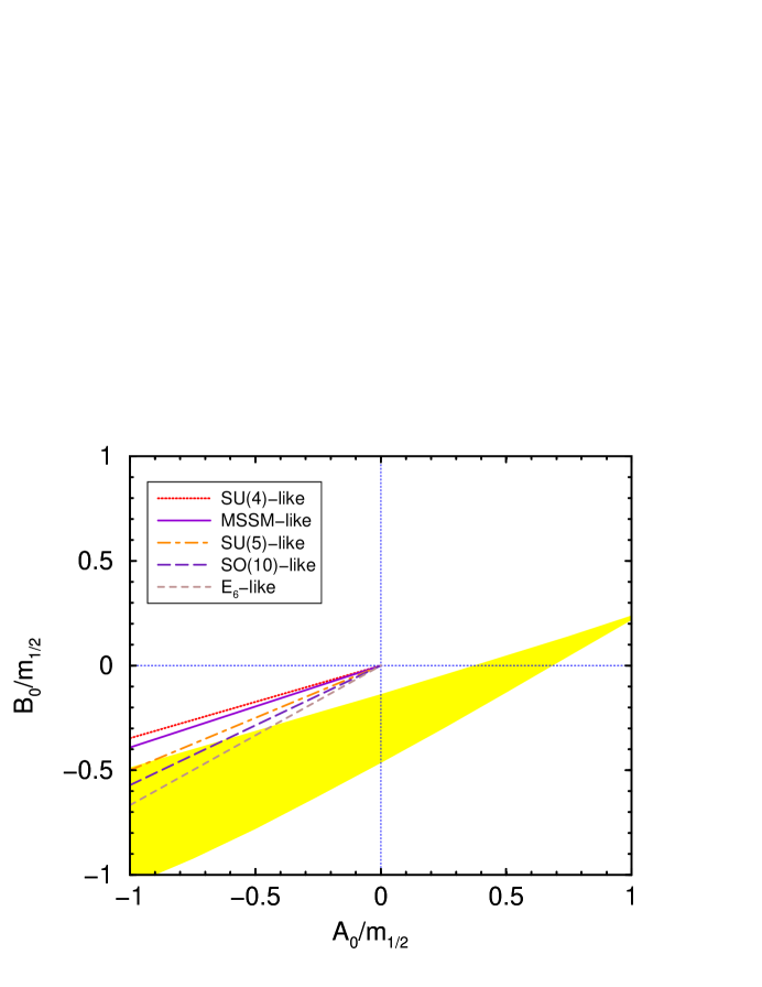
Figure 5: The $B_{0}/m_{1/2}$ vs. $A_{0}/m_{1/2}$ plane is divided into three regions, according to whether $\mu$ must be positive (upper unshaded), $\mu$ must be negative (lower unshaded), or $\mu$ can have either sign (shaded). The top and bottom quark masses and $\alpha_{3}$ are allowed to vary over the entire ranges indicated in eq. (17)-(19). Universal gaugino masses are restricted by $m_{1/2}<400$ GeV and universal scalar masses lie in the range $0<m_{0}^{2}/m_{1/2}^{2}<1$. All values of $\tan\beta$ leading to correct EWSB, perturbative couplings up to $M_{U}$, and charged superpartners heavier than 100 GeV are allowed. For comparison, the approximate boundary condition ratio predictions of various model frameworks as described in the text are indicated by lines.

In the upper unshaded region including $A_{0}=B_{0}=0$, the sign of $\mu$ is definitely positive. In the lower unshaded region, the sign of $\mu$ is definitely negative. In the intermediate (yellow) shaded region, the sign of $\mu$ can be either positive or negative, depending on the values of supersymmetric dimensionless couplings. The extent of this region was maximized by scanning over the full allowed range of top and bottom masses and QCD coupling, as in eqs. (17)-(19), as well as including all $m_{1/2}<400$ GeV and $0<m_{0}^{2}/m_{1/2}^{2}<1$. (The region will grow very slowly as the maximum allowed $m_{1/2}$ is increased.) Also shown are lines corresponding to the boundary conditions of the different types of models as described above. In the MSSM-like and $SU(5)$-like cases, $A_{0t}/B_{0}$ and $A_{0b}/B_{0}$ and $A_{0\tau}/B_{0}$ are slightly different, so the more important factor $A_{0t}/m_{1/2}$ is used. We learn the following general lessons. First, if the $M_{\rm X}\rightarrow M_{\rm U}$ corrections are not too large, then $\mu$ must be positive in all cases. Second, in models with larger corrections, gauge groups in which the top and bottom quarks are in larger representations than the Higgs fields require positive $\mu$, while the highly unified groups $E_{6}$ and $SO(10)$ can sometimes allow either sign of $\mu$.

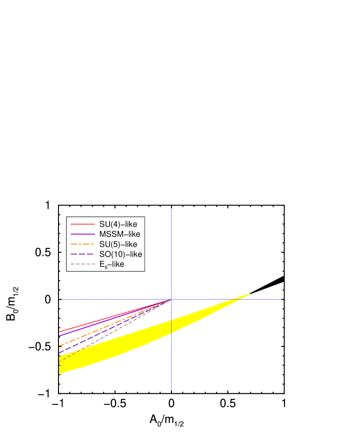
Figure 6: As in Figure 5, but now taking the top quark mass fixed at its central value, and $m_{1/2}=400$ GeV with $m_{0}^{2}=0.5m_{1/2}^{2}$. The upper unshaded region requires $\mu>0$; the lower unshaded region requires $\mu<0$; the lighter shaded region allows $\mu$ of either sign; and the black region at the right allows no solutions. This shows the improvement that could follow from knowing the top quark mass accurately and the sfermion masses with reasonable precision.

Someday, the top-quark mass will be better known, and its relation to the top Yukawa coupling in supersymmetry more accurately computed. Furthermore, measurements of the sparticle spectrum will enable determination of $m_{1/2}$, $m_{0}$. Figure 6 depicts how the situation will improve, now assuming as fixed the present central value for the top mass with the one-loop supersymmetric corrections, and $m_{0}^{2}$ equal to $0.5m^{2}_{1/2}$. As shown, the region in which the sign of $\mu$ is not determined by $A_{0}/m_{1/2}$ and $B_{0}/m_{1/2}$ shrinks significantly in this case compared to fig. 5. It will shrink even more if $\tan\beta$ is measured. This represents a concrete benefit of an accurate measurement of the top-quark mass and couplings in testing our ideas of high-scale physics.

The fact that the $\mu$-term is apparently of the same order of magnitude as the supersymmetry-breaking soft terms is a major puzzle within the MSSM. Therefore one should question whether the origin of the $b$-term might be qualitatively different from that of the other soft terms, so that the boundary condition $B_{0}=0$ should not be applied. However, the origin of the $b$-term cannot be completely arbitrary, or else one would expect CP-violating couplings in the neutralino and chargino sector. In any case, with a theory for the origin of the $b$-term one can simply look at the plots above with $B_{0}/m_{1/2}$ displaced by the appropriate amount.

One general strategy for solving the $\mu$ problem relies on replacing it by the VEV of an additional gauge singlet field [27]. This allows all dimensionful parameters to be banned from the superpotential, which now includes instead of the $\mu$-term:

$$W=-\lambda SH_{u}^{0}H_{d}^{0}+\ldots$$ (35)

where the ellipses may refer to a self-coupling of $S$ and/or couplings of $S$ to other non-MSSM fields. The corresponding supersymmetry-breaking Lagrangian is

$$-{\cal L}_{\rm soft}=-a_{\lambda}SH_{u}^{0}H_{d}^{0}+m_{S}^{2}|S|^{2}+\ldots$$ (36)

Consider the limit of small $\lambda$, so that the resulting theory describes a nearly unmixed singlino and MSSM neutralinos. Then when $S$ gets its VEV, one has effectively

$$\mu=\lambda\langle S\rangle;\qquad b=a_{\lambda}\langle S\rangle.$$ (37)

So all of the above analysis can be repeated with $b/\mu$ replaced by $a_{\lambda}/\lambda$. The RG equations for the scalar cubic couplings are given by adding a term $2a_{\lambda}\lambda$ to each of eqs. (20)-(22), and replacing eq. (23) by

$$16\pi^{2}{d\over dt}(a_{\lambda}/\lambda) = 6g_{2}^{2}M_{2}+{6\over 5}g_{1}^{2}M_{1}+6a_{t}y_{t}+6a_{b}y_{b}+2a_{\tau}y_{\tau}+8a_{\lambda}\lambda$$ (38)

where the effects of other couplings of $S$ on its anomalous dimension are omitted. The last term is just a damping term and cannot change the sign of $a_{\lambda}/\lambda$. In the limit of weakly coupled $S$, the additional terms are inconsequential and the preceding analysis goes through without change. Of course, one must still look at the details of the particular model to decide whether it can be viable.

The above results were obtained assuming that gaugino masses are unified to a common value $m_{1/2}$ and that scalar squared masses are unified to $m^{2}_{0}$. The dependence on the latter assumption is not very strong, as the non-holomorphic scalar squared masses mainly enter into the determination of the sign of $\mu$ through their influence on $\tan\beta$, and all values of $\tan\beta$ were considered. The assumption of gaugino mass unification is stronger, since non-unified gaugino masses will affect the running of $b/\mu$ and $a_{f}/y_{f}$ in different ways. However, gaugino masses can be reconstructed with good accuracy from future measurements of gluino, neutralino and chargino masses, so a similar analysis can be repeated for the case that gaugino mass unification is badly violated. The top and bottom Yukawa couplings may well be modified from their extrapolated behavior at high mass scales, but the dependence of Yukawa couplings on the RG evolution comes mainly from lower scales anyway in models of gaugino mass dominance.

After the discovery of supersymmetry, it will be an important challenge to connect measured properties of the superpartners to candidate theories of supersymmetry breaking. In fact, there are already a couple of weak indirect hints from experiment which may suggest that if superpartners are not too heavy and gaugino masses have a common phase, then $\mu$ should be positive in the standard convention. First, it is often easier to accommodate constraints on $b\rightarrow s\gamma$ within simple model frameworks if $\mu>0$ [28]. Second, the recent measurement [29] of the muon magnetic dipole moment also favors this sign [30, 31] if $\tan\beta$ is not too small and superpartners are not too heavy. While caution is certainly called for before hailing the muon $g-2$ discrepancy as evidence in favor of supersymmetry, it should be remembered that many models with $\mu<0$ are ruled out by the data at a far higher confidence level. In any case, these considerations highlight the importance of understanding the sign of $\mu$ as a consequence of theory, rather than merely an input parameter. As I have emphasized in this paper, the theory of the mechanism of supersymmetry breaking can predict the sign of $\mu$ in addition to the more obvious mass hierarchies in the sparticle spectrum.

Acknowledgements: This work was supported in part by the National Science Foundation grant number PHY-9970691. I thank Graham Kribs, Martin Schmaltz and James Wells for helpful conversations.

References

- [1] H.E. Haber and G.L. Kane, Phys. Rept. 117, 75 (1985); J.F. Gunion and H.E. Haber, Nucl. Phys. B 272, 1 (1986) [Erratum-ibid. B 402, 567 (1986)].
- [2] S.P. Martin, “A Supersymmetry Primer,” hep-ph/9709356.
- [3] J. Ellis, C. Kounnas and D. V. Nanopoulos, Nucl. Phys. B 247, 373 (1984); J. Ellis, A. B. Lahanas, D. V. Nanopoulos and K. Tamvakis, Phys. Lett. B 134, 429 (1984), A. B. Lahanas and D. V. Nanopoulos, Phys. Rept. 145, 1 (1987).
- [4] J. L. Lopez, D. V. Nanopoulos and A. Zichichi, Phys. Rev. D 49, 343 (1994); Int. J. Mod. Phys. A 10, 4241 (1995).
- [5] D. E. Kaplan, G. D. Kribs and M. Schmaltz, Phys. Rev. D 62, 035010 (2000).
- [6] Z. Chacko, M. A. Luty, A. E. Nelson and E. Ponton, JHEP 0001, 003 (2000).
- [7] M. Schmaltz and W. Skiba, Phys. Rev. D 62, 095005 (2000); M. Schmaltz and W. Skiba, Phys. Rev. D 62, 095004 (2000).
- [8] T. Kobayashi and K. Yoshioka, Phys. Rev. Lett. 85, 5527 (2000).
- [9] Z. Chacko and M. A. Luty, JHEP 0105, 067 (2001).
- [10] C. Csaki, J. Erlich, C. Grojean and G. D. Kribs, hep-ph/0106044.
- [11] H. C. Cheng, D. E. Kaplan, M. Schmaltz and W. Skiba, hep-ph/0106098.
- [12] J. Hisano and M. Shifman, Phys. Rev. D 56, 5475 (1997); I. Jack and D.R.T. Jones, Phys. Lett. B 415, 383 (1997).
- [13] K. S. Babu, C. Kolda and F. Wilczek, Phys. Rev. Lett. 77, 3070 (1996); M. Dine, Y. Nir and Y. Shirman, Phys. Rev. D 55, 1501 (1997); S. Dimopoulos, S. Thomas and J. D. Wells, Nucl. Phys. B 488, 39 (1997).
- [14] J. A. Bagger, K. Matchev, D. M. Pierce and R. Zhang, Phys. Rev. D 55, 3188 (1997).
- [15] R. Rattazzi and U. Sarid, Nucl. Phys. B 501, 297 (1997); E. Gabrielli and U. Sarid, Phys. Rev. Lett. 79, 4752 (1997); Phys. Rev. D 58, 115003 (1998).
- [16] A. Mafi and S. Raby, Phys. Rev. D 63, 055010 (2001) [hep-ph/0009202].
- [17] S. P. Martin and M. T. Vaughn, Phys. Rev. D 50, 2282 (1994); Y. Yamada, Phys. Rev. D 50, 3537 (1994); I. Jack and D.R.T. Jones, Phys. Lett. B 333, 372 (1994).
- [18] I. Jack et al, Phys. Rev. D 50, 5481 (1994).
- [19] W. Siegel, Phys. Lett. B 84, 193 (1979); D. M. Capper, D. R. Jones and P. van Nieuwenhuizen, Nucl. Phys. B 167, 479 (1980).
- [20] D. M. Pierce, J. A. Bagger, K. Matchev and R. Zhang, Nucl. Phys. B 491, 3 (1997).
- [21] R. Zhang, Phys. Lett. B 447, 89 (1999).
- [22] J. R. Espinosa and R. Zhang, Nucl. Phys. B 586, 3 (2000). See also M. Carena, H. E. Haber, S. Heinemeyer, W. Hollik, C. E. Wagner and G. Weiglein, Nucl. Phys. B 580, 29 (2000) and references therein.
- [23] D. J. Castaño, E. J. Piard and P. Ramond, Phys. Rev. D 49, 4882 (1994).
- [24] D. E. Groom et al. [Particle Data Group Collaboration], Eur. Phys. J. C 15, 1 (2000).
- [25] S. P. Martin and J. D. Wells, [hep-ph/0011382], Phys. Rev. D to appear.
- [26] R. Barbieri, L. Hall and A. Strumia, Nucl. Phys. B 445, 219 (1995).
- [27] H. P. Nilles, M. Srednicki and D. Wyler, Phys. Lett. B 120, 346 (1983), J. M. Frere, D. R. Jones and S. Raby, Nucl. Phys. B 222, 11 (1983), J. P. Derendinger and C. A. Savoy, Nucl. Phys. B 237, 307 (1984), J. Ellis, et al., Phys. Rev. D 39, 844 (1989), M. Drees, Int. J. Mod. Phys. A 4, 3635 (1989), S. A. Abel, S. Sarkar and I. B. Whittingham, Nucl. Phys. B 392, 83 (1993), S. F. King and P. L. White, Phys. Rev. D 52, 4183 (1995), U. Ellwanger, M. Rausch de Traubenberg, C. A. Savoy, Nucl. Phys. B492 (1997) 21, M. Bastero-Gil and S. F. King, Phys. Lett. B 423, 27 (1998), U. Ellwanger and C. Hugonie, Eur. Phys. J. C5 (1998) 723; hep-ph/9812427, C. Panagiotakopoulos and K. Tamvakis, Phys. Lett. B 469, 145 (1999), A. Dedes, C. Hugonie, S. Moretti and K. Tamvakis, Phys. Rev. D 63, 055009 (2001).
- [28] H. Baer, M. Brhlik, D. Castaño and X. Tata, Phys. Rev. D 58, 015007 (1998), Phys. Rev. D 61, 095004 (2000), K. T. Mahanthappa and S. Oh, Phys. Rev. D 62, 015012 (2000), G. Degrassi, P. Gambino and G. F. Giudice, JHEP 0012, 009 (2000), M. Carena, D. Garcia, U. Nierste and C. E. Wagner, Phys. Lett. B 499, 141 (2001), J. Ellis, T. Falk, G. Ganis, K. A. Olive and M. Srednicki, hep-ph/0102098.
- [29] H. N. Brown et al. [Muon g-2 Collaboration], Phys. Rev. Lett. 86, 2227 (2001).
- [30] J. L. Lopez, D. V. Nanopoulos and X. Wang, Phys. Rev. D 49, 366 (1994), T. Moroi, Phys. Rev. D 53, 6565 (1996) [Erratum-ibid. D 56, 4424 (1996)], M. Carena, G. F. Giudice and C. E. Wagner, Phys. Lett. B 390, 234 (1997) T. Ibrahim and P. Nath, Phys. Rev. D 61, 095008 (2000), T. Ibrahim and P. Nath, Phys. Rev. D 62, 015004 (2000), G. Cho, K. Hagiwara and M. Hayakawa, Phys. Lett. B 478, 231 (2000), U. Chattopadhyay, D. K. Ghosh and S. Roy, Phys. Rev. D 62, 115001 (2000), M. Drees, Y. G. Kim, T. Kobayashi and M. M. Nojiri, Phys. Rev. D 63, 115009 (2001).
- [31] J. L. Feng and K. T. Matchev, Phys. Rev. Lett. 86, 3480 (2001), L. L. Everett, G. L. Kane, S. Rigolin and L. Wang, Phys. Rev. Lett. 86, 3484 (2001), E. A. Baltz and P. Gondolo, Phys. Rev. Lett. 86, 5004 (2001), U. Chattopadhyay and P. Nath, hep-ph/0102157, S. Komine, T. Moroi and M. Yamaguchi, Phys. Lett. B 506, 93 (2001), J. Ellis, D. V. Nanopoulos and K. A. Olive, Phys. Lett. B 508, 65 (2001), R. Arnowitt, B. Dutta, B. Hu and Y. Santoso, Phys. Lett. B 505, 177 (2001), K. Choi, K. Hwang, S. K. Kang, K. Y. Lee and W. Y. Song, hep-ph/0103048, S. P. Martin and J. D. Wells, Phys. Rev. D 64, 035003 (2001), S. Komine, T. Moroi and M. Yamaguchi, Phys. Lett. B 507, 224 (2001), S. Baek, P. Ko and H. S. Lee, hep-ph/0103218, H. Baer, C. Balazs, J. Ferrandis and X. Tata, hep-ph/0103280, M. Graesser and S. Thomas, hep-ph/0104254, Z. Chacko and G. D. Kribs, hep-ph/0104317.