The evolution and persistence of dumbbells

Abstract:

We use large-scale numerical simulations to study the formation and evolution of non-topological defects in a generalized electroweak phase transition described by the Glashow-Salam-Weinberg model without fermions. Such defects include dumbbells, comprising a pair of monopoles joined by a segment of electroweak string. These exhibit complex dynamics, with some shrinking under the string tension and others growing due to the monopole-antimonopole attractions between near neighbours. We estimate the range of parameters where the network of dumbbells persists, and show that this region is narrower than the region within which infinite straight electroweak strings are perturbatively stable.

1 Introduction

The formation of topological defects in any phase transition depends on the existence of a non-trivial, low-order homotopy group of the broken-symmetry vacuum manifold [1, 2]. Even in the absence of this, dynamically stable non-topological defects are sometimes still possible, but are usually assumed to be too weakly stable to lead to a lasting network. A particularly interesting case is non-topological strings where at least one example is known (semilocal strings [3, 4]) in which a space-spanning network of strings can develop from the growth and joining of short string segments formed at the phase transition [5]. Semilocal strings are a special case of electroweak strings [6, 7, 8].

The stability of electroweak strings has been analyzed in some detail in the Glashow-Salam-Weinberg (GSW) model. In the absence of fermions the theory is determined, up to scalings, by only two parameters: the weak mixing angle ${\theta_{{{\rm W}}}}$, and $\beta$ which is the square of the ratio of the Higgs and $Z$-boson masses (the observed value for the actual electroweak model is ${\rm sin}^{2}{\theta_{{{\rm W}}}}\simeq 0.23$, and the precise value of $\beta$ has not yet been determined but is almost certainly greater than one).

In the case of interest here, the topology of the vacuum manifold is the three-sphere $S^{3}$, which does not support persistent topological defects in 3+1 dimensional spacetime, but there are grounds for expecting non-topological defects to form. In the limit ${\theta_{{{\rm W}}}}=\pi/2$ we recover the so-called semilocal model, whose $S^{3}$ vacuum manifold is known to support stable non-topological strings from both analytical [3, 4] and numerical [5] work. In particular, a straight infinite semilocal string can be seen as a Nielsen-Olesen (NO) $\mathop{\rm{}U}(1)$ vortex [9], embedded in a higher group $\mathop{\rm SU}(2)_{{\rm global}}\times\mathop{\rm{}U}(1)_{{\rm local}}$. Note, however, that in the semilocal string case, we can define a quantity (the winding number) which, although not a topological invariant in the usual sense, is topologically conserved.

The embedding of NO vortices into the full electroweak symmetry $\mathop{\rm SU}(2)_{L}\times\mathop{\rm{}U}(1)_{{\rm{\scriptscriptstyle Y}}}$ leads to $Z$-strings and $W$-strings (see ref. [8]). Although $W$-strings are expected to be unstable, analysis of infinite axially-symmetric $Z$-strings has shown the existence of a parameter regime where they are perturbatively stable [7, 10]. But these $Z$-strings are genuinely non-topological, there is no quantity which is topologically conserved.

In this paper we will consider the evolution and persistence of these genuine non-topological defects in a generalized GSW model, spanning all values of $\beta$ and ${\theta_{{{\rm W}}}}$, using numerical methods. Isolated, infinite, axially-symmetric $Z$-string configurations will not be formed in a realistic system, but configurations consisting of monopole-antimonopole pairs joined by $Z$-string segments, named dumbbells by Nambu [6], are certainly possible. Isolated dumbbells are expected to collapse under the string tension, at least in the absence of rotation, jittering or magnetic fields [6, 11, 12]. Of particular interest is the question of whether there is a region of parameter space in which the density of dumbbells is sufficiently high so that they are able to generate a persistent network of strings by building up longer segments from the merging of shorter ones due to interaction of neighbouring monopoles, as has been found in the semilocal case [5]. This region of parameter space will lie far from the measured values for ${\theta_{{{\rm W}}}}$ and $\beta$, but the mere existence of this region is striking. It shows that in models close to real physical ones, completely non-topological defect networks can form and persist, so in extensions of the GSW model (to higher symmetry groups or extra fields), or models with a background magnetic field [12], or even models in which topological (semilocal) defects exist in some limit, non-topological defects cannot be ruled out immediately.

Moreover, the study of the dynamics of dumbbells can be of interest in computing other early universe features, such as the primordial magnetic field helicity [15, 16].

2 The model

The bosonic sector of the GSW electroweak model describes an $\mathop{\rm SU}(2)_{L}\times\mathop{\rm{}U}(1)_{{\rm{\scriptscriptstyle Y}}}$ invariant theory with a scalar field $\Phi$ in the fundamental representation of $\mathop{\rm SU}(2)_{L}$, with lagrangian

$$\mathcal{L}=\left|D_{\mu}\Phi\right|^{2}-\frac{1}{4}W^{a}_{\mu\nu}W^{a\mu\nu}-\frac{1}{4}Y_{\mu\nu}Y^{\mu\nu}-\lambda\left(\Phi\Phi^{\dagger}-\frac{\eta^{2}}{2}\right)^{2}.$$ (1)

The covariant derivative is given by

$$D_{\mu}\equiv\partial_{\mu}-\frac{ig_{{\rm{\scriptscriptstyle W}}}}{2}\tau^{a}W^{a}_{\mu}-\frac{ig_{{\rm{\scriptscriptstyle Y}}}}{2}Y_{\mu}\,,\qquad a=1,2,3\,,$$ (2)

where $\Phi$ is a complex doublet, $\tau^{a}$ are the Pauli matrices, $W_{\mu}^{a}$ is a $\mathop{\rm SU}(2)$ gauge field and $Y_{\mu}$ is a $\mathop{\rm{}U}(1)$ gauge field. The field strengths associated with these gauge fields are

$$W_{\mu\nu}^{a} = \partial_{\mu}W^{a}_{\nu}-\partial_{\nu}W^{a}_{\mu}+g_{{\rm{\scriptscriptstyle W}}}\epsilon^{abc}W_{\mu}^{b}W_{\nu}^{c}\,;$$

$$Y_{\mu\nu} = \partial_{\mu}Y_{\nu}-\partial_{\nu}Y_{\mu}\,,$$ (3)

respectively, and there is no distinction between upper and lower group indices ($\epsilon^{123}=1$).

When the scalar field acquires a non-zero vacuum expectation value the symmetry breaks from $\mathop{\rm SU}(2)_{L}\times\mathop{\rm{}U}(1)_{{\rm{\scriptscriptstyle Y}}}$ to $\mathop{\rm{}U}(1)_{{\rm e.m.}}$, leaving a massive scalar field ($m_{H}=\sqrt{2\lambda}\eta$), a massless neutral photon ($A_{\mu}$), a massive neutral $Z$-boson ($Z_{\mu}$, $m_{{{\rm z}}}=g_{{{\rm z}}}\eta/2\equiv l_{v}^{-1}$, where $g_{{{\rm z}}}=\sqrt{g_{{\rm{\scriptscriptstyle Y}}}^{2}+g_{{\rm{\scriptscriptstyle W}}}^{2}}$), and two massive charged $W$-bosons ($W_{\mu}^{\pm}$, $m_{W}=g_{{\rm{\scriptscriptstyle W}}}\eta/2$).

We make the following rescaling

$$\Phi\to\frac{\eta}{\sqrt{2}}\Phi\,,\qquad x_{\mu}\to\frac{\sqrt{2}}{g_{{{\rm z}}}\eta}x_{\mu}\,,\qquad g_{\rm{\scriptscriptstyle Y}}Y_{\mu}\to\frac{g_{{{\rm z}}}\eta}{\sqrt{2}}Y_{\mu}\,,\qquad g_{\rm{\scriptscriptstyle W}}W^{a}_{\mu}\to\frac{g_{{{\rm z}}}\eta}{\sqrt{2}}W^{a}_{\mu}\,,$$ (4)

to choose $l_{v}$ as the unit of length, $\eta$ as the unit of energy, and the $Z$-charge of the scalar field ($g_{{{\rm z}}}$) as the unit of charge (up to numerical factors). This brings the classical field equations to the form

$$D^{\mu}D_{\mu}\Phi+\frac{2\lambda}{g_{{{\rm z}}}^{2}}\left(\Phi\Phi^{\dagger}-1\right)\Phi = 0\,;$$

$$\partial_{\nu}W^{\mu\nu a}+\epsilon^{abc}W_{\nu}^{b}W^{\mu\nu c} = \frac{i}{2}{\rm cos}^{2}\,{\theta_{{{\rm W}}}}\left[\Phi^{\dagger}\tau^{a}D^{\mu}\Phi-\left(D^{\mu}\Phi\right)^{\dagger}\tau^{a}\Phi\right];$$

$$\partial_{\nu}Y^{\mu\nu} = \frac{i}{2}{\rm sin}^{2}\,{\theta_{{{\rm W}}}}\left[\Phi^{\dagger}D^{\mu}\Phi-\left(D^{\mu}\Phi\right)^{\dagger}\Phi\right],$$ (5)

where the weak mixing angle is given by ${\rm tan}\,{\theta_{{{\rm W}}}}\equiv g_{{\rm{\scriptscriptstyle Y}}}/g_{{\rm{\scriptscriptstyle W}}}$, and now

$$W_{\mu\nu}^{a} \equiv \partial_{\mu}W_{\nu}^{a}-\partial_{\nu}W_{\mu}^{a}+\epsilon^{abc}W_{\mu}^{b}W_{\nu}^{c}\,;$$

$$D_{\mu} \equiv \partial_{\mu}-\frac{i}{2}\tau^{a}W_{\mu}^{a}-\frac{i}{2}Y_{\mu}\,.$$ (6)

Typically the $Z$- and $A$-fields are expressed in the unitary gauge $\Phi^{T}=(0,1)$, but this choice is not well suited to work with defects. Instead, when there are points in space-time with $|\Phi|\neq 1$, it is customary to use a more general definition of these fields which depends on the Higgs field configuration at each point [6], namely,

$$Z_{\mu} \equiv {\rm cos}\,{\theta_{{{\rm W}}}}\,n^{a}(x)\,W^{a}_{\mu}-{\rm sin}\,{\theta_{{{\rm W}}}}\,Y_{\mu}\,;$$

$$A_{\mu} \equiv {\rm sin}\,{\theta_{{{\rm W}}}}\,n^{a}(x)\,W^{a}_{\mu}+{\rm cos}\,{\theta_{{{\rm W}}}}Y_{\mu}\,,$$ (7)

where

$$n^{a}(x)\equiv-\frac{\Phi^{\dagger}(x)\tau^{a}\Phi(x)}{\Phi^{\dagger}(x)\Phi(x)}\,,$$ (8)

is a unit vector by virtue of the Fierz identity $\sum_{a}\left(\Phi^{\dagger}\tau^{a}\Phi\right)^{2}=\left(\Phi^{\dagger}\Phi\right)^{2}$. There are also several possible definitions for the field strengths (see, e.g. ref. [13] for a discussion of this point); in our simulations we will use

$$Z_{\mu\nu} = {\rm cos}{\theta_{{{\rm W}}}}\,n^{a}(x)\,W_{\mu\nu}^{a}-{\rm sin}{\theta_{{{\rm W}}}}\,Y_{\mu\nu}\,;$$

$$A_{\mu\nu} = {\rm sin}{\theta_{{{\rm W}}}}\,n^{a}(x)\,W_{\mu\nu}^{a}+{\rm cos}{\theta_{{{\rm W}}}}\,Y_{\mu\nu}\,.$$ (9)

Note that eqs. (7) to (9) reduce to the usual definitions away from the defect cores. We work in flat space and in the temporal gauge ($W_{0}^{a}=Y_{0}=0$ for $a=1,2,3$) so $D_{0}\Phi=\partial_{0}\Phi$. With this gauge choice, Gauss’s Law becomes

$$-\partial_{j}(\partial_{0}Y_{j}) = \frac{i}{2}{\rm sin}^{2}{\theta_{{{\rm W}}}}\left[\Phi^{\dagger}\partial_{0}\Phi-(\partial_{0}\Phi)^{\dagger}\Phi\right];$$

$$-\partial_{j}(\partial_{0}W_{j}^{a})-\epsilon^{abc}W_{j}^{b}\partial_{0}W_{j}^{c} = \frac{i}{2}{\rm cos}^{2}{\theta_{{{\rm W}}}}\left[\Phi^{\dagger}\tau^{a}\partial_{0}\Phi-(\partial_{0}\Phi)^{\dagger}\tau^{a}\Phi\right],$$ (10)

(with $j=1,2,3$) which is then used to test the stability of the code.

As noted above, the ${\rm sin}^{2}{\theta_{{{\rm W}}}}=1$ case reduces to the semilocal case, where absolutely stable defects are known to exist. Setting one of the Higgs fields to zero further reduces this to the abelian Higgs model. We are able to use our knowledge of these systems, as well as the behaviour of artificially constructed infinite axially-symmetric $Z$-strings at various points in parameter space, to check the validity of our simulation code.

3 Numerical simulations

The equations of motion eq. (5) are discretized using a naïve staggered leapfrog method, where both the scalar and gauge fields are associated with lattice points. This procedure is the easiest to relate to previous work on semilocal defects [5], and we expect to have a fairly good picture at the scales we are interested in. A comparison to a link-variable discretization [17] of eq. (5) in the semilocal case (${\theta_{{{\rm W}}}}=\pi/2$) shows that the changes from using a lattice implementation instead of this naïve one are well within the other uncertainties; see the appendix for a full analysis. The simulations are performed on a periodic cubic lattice whose time step is $0.2$ times the spatial step $\Delta t=0.2\Delta x$ ($c=1$), with ad hoc numerical viscosity terms added to each equation ($\gamma\,\dot{\Phi}$, $\gamma\,\dot{Y}$ and $\gamma\,\dot{W}^{a}$ respectively) to reduce the system’s relaxation time. The expansion rate in an expanding universe would play this role, albeit as a time-dependent factor $\gamma(t)$ typically scaling as $1/t$. Several different values of $\gamma$ were tested, and generated very similar behaviour; throughout this work we use $\gamma=0.5$.

Two different strategies for setting the initial configurations were considered:

• Set all initial field velocities to zero and throw down random scalar field phases at every lattice point; average the field at each point with its 6 nearest neighbours and normalize the fields to the vacuum value ($|\Phi|^{2}=1$ as $\eta$ has been rescaled out) iteratively (50 times), to get a smoother configuration; using these scalar field values, choose the initial values of the gauge fields to be

  $$Y_{\mu} = 0$$

  $$W_{\mu}^{1} = 2\left(\psi_{1}\nabla_{j}\psi_{4}-\psi_{4}\nabla_{j}\psi_{1}+\psi_{3}\nabla_{j}\psi_{2}-\psi_{2}\nabla_{j}\psi_{3}\right)$$

  $$W^{2}_{\mu} = 2\left(\psi_{3}\nabla_{j}\psi_{1}-\psi_{1}\nabla_{j}\psi_{3}+\psi_{4}\nabla_{j}\psi_{2}-\psi_{2}\nabla_{j}\psi_{4}\right)$$

  $$W^{3}_{\mu} = 2\left(\psi_{1}\nabla_{j}\psi_{2}-\psi_{2}\nabla_{j}\psi_{1}+\psi_{4}\nabla_{j}\psi_{3}-\psi_{3}\nabla_{j}\psi_{4}\right)$$ (11)

  where $\Phi^{T}=(\psi_{1}+i\,\psi_{2},\psi_{3}+i\,\psi_{4})$, pseudo-minimizing the energy as in ref. [14]. Note, however, that in the present case, the system does have enough gauge fields to cancel completelly the gradient energy. In fact, the configuration (11) sets to zero the gradient energy, the potential energy and the field-strength energy corresponding to the $\mathop{\rm{}U}(1)$ gauge field, leaving the $\mathop{\rm SU}(2)$ field-strength energy as the only non-zero term.

• Set all fields to zero, and also gauge field velocities to zero ($\Phi=W^{a}_{\mu}=\dot{W}^{a}_{\mu}=Y_{\mu}=\dot{Y}_{\mu}=0$); provide some initial (smoothed) random velocities to the scalar field ($\dot{\Phi}\neq 0$) following the general procedure as above. This initial configuration would be closer to that appropriate to a bubble nucleation scheme.

The overall results in our simulations did not show qualitatively different behaviour between the two cases. Indeed, in the first case the gauge field energy pseudo-minimization was ineffective enough that the scalar field typically began by climbing up the potential, restoring the symmetric phase, and rolled down again later. Previous experience with semilocal strings also shows that the results are fairly insensitive to the specific way initial conditions are implemented. For all these reasons, we chose the second initial configuration ($b$) for our investigations.

Interpreting simulations of electroweak string networks is more complicated than in the $\mathop{\rm{}U}(1)$ cosmic string case. As in the semilocal case, electroweak strings are non-topological, and in this case there is no well-defined winding number, which makes identification of strings a more difficult task. We follow the strategy proposed in ref. [14] in order to study string formation: the system is evolved forward in time and we compute a set of gauge-invariant quantities at each time step, namely the $Z$- and the $A$-field strengths given by eq. (9) and the modulus of the scalar field ($|\Phi|$). String formation is then observed by visualizing isosurfaces in the $Z$-field strength ($\sqrt{\frac{1}{2}Z_{ij}Z^{ij}}$) and in the scalar field modulus.

After the rescaling eq. (4), it becomes clear that the only free parameters in our model are $\beta$ ($\beta\equiv m_{H}^{2}/m_{{{\rm z}}}^{2}=8\lambda/g_{{\rm z}}^{2}$) and ${\theta_{{{\rm W}}}}$. It is well known that with ${\theta_{{{\rm W}}}}=\pi/2$ and $\beta<1$ we have semilocal strings that are stable [4], and numerical simulations show segment formation and linkage [5]. Moreover, for ${\rm sin}^{2}{\theta_{{{\rm W}}}}\lesssim 1$, $\beta<1$, there is a regime, albeit a rather narrow one, where infinitely long strings are perturbatively stable [7, 10]. Bearing these results in mind, the parameter space investigated in our simulations was $0.9\leq{\rm sin}^{2}{\theta_{{{\rm W}}}}\leq 1$ and $0.05\leq\beta\leq 1.5$.

Simulation and visualization were performed on $64^{3}$, $128^{3}$ and $256^{3}$ lattices using the Cray T3E at NERSC, and high-performance computing facilities at University of Sussex and University of Groningen. Our quoted results all come from $256^{3}$ simulations.

4 Results

To test our code, we began by reproducing known results for cosmic and semilocal string networks, and for infinitely long, axially-symmetric $Z$-strings (made possible by our periodic boundary conditions as long as strings are simulated in pairs to keep the net flux equal to zero) in both the stable and unstable regimes, in particular verifying that the $Z$-strings disappeared in the unstable regime.

Having checked the code, we then ran it for values of the two free parameters ($\theta_{W},\beta$) throughout the regime of interest, using the same initial conditions for each parameter pair. We chose to carry out one large simulation at each point in parameter space rather than many smaller ones, which gives improved dynamical range. As expected, after an initial transient, the typical configuration observed is a dumbbell — a segment of electroweak string joining a monopole/antimonopole pair. By continuity, for parameter values sufficiently close to the stable semilocal case we expect the monopole interactions to lead to the joining of strings to form longer segments.

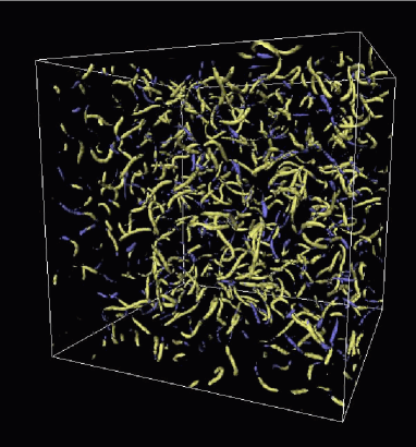
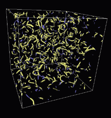
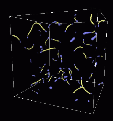
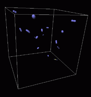
Figure 1: Isosurfaces of the $Z$- and $A$-magnetic field strengths for two different simulations, shown as the light and dark colour respectively. The left panels show $\beta=0.1$, ${\rm sin}^{2}{\theta_{{{\rm W}}}}=0.994$ (persistent regime) and the right ones $\beta=0.5$, ${\rm sin}^{2}{\theta_{{{\rm W}}}}=0.995$ (non-persistent regime). The top row is at an early stage of the simulation $t=50$, while the lower is at the end $t=200$. Note that in the first case there remain some long strings at the end of the simulation and connection can still occur. In the second all the defects are about to disappear.

The simulations show that some short segments of $Z$-string do join as expected. The joining rate is, however, lower than in the semilocal case, and decreases both as ${\rm sin}^{2}{\theta_{{{\rm W}}}}$ is decreased and as $\beta$ is increased. Thus, some segments which would eventually join in the semilocal case are seen instead to collapse in the electroweak case due to string tension. This is not surprising: in the semilocal case, we have global monopoles at the string ends, which have divergent scalar gradient energy and are more efficient at finding neighbouring monopoles. In the electroweak case, the monopoles at the string ends are proper magnetic monopoles, and the scalar gradients are cancelled much more efficiently by gauge fields. As ${\rm sin}^{2}{\theta_{{{\rm W}}}}\to 1$ the cores become larger, and eventually overlap, making segments join. But as we move away from the semilocal case, the cores become smaller and the joining becomes less important.

Figure 1 shows timeslices of two typical simulations, with the different colours corresponding to the $A$- and $Z$-field strengths.

The $Z$-field has a string-like form, whereas the $A$-field at the string ends is a spherical shell, corresponding to spherical magnetic monopoles. The $A$-field morphology can also be tube-like, denoting interaction between monopoles, illustrating the complexity of the overall dynamics. The interplay between string tension and monopole-antimonopole attraction causes some strings to shrink until they disappear, and others join to form longer strings.

To compare the number of defects in the semilocal and electroweak cases, we plot the number of lattice sites with $Z$-magnetic field strength ($\sqrt{\frac{1}{2}Z_{ij}Z^{ij}}$) greater than 25% of the maximum field strength found in the core of a NO string with the same value of $\beta$ (see figure 2). The number of lattice sites, and hence length of string, decreases more rapidly in the electroweak case as either ${\rm sin}^{2}{\theta_{{{\rm W}}}}$ decreases or $\beta$ grows.

Figure 2: The number of lattice points with $Z$-field strength ($\sqrt{\frac{1}{2}Z_{ij}Z^{ij}}$) bigger than $25\%$ of the maximum (core) value in the NO case, calculated in a series of $256^{3}$ simulations, for $\beta=0.3$. The different lines correspond to different choices of the weak mixing angle ${\theta_{{{\rm W}}}}$ (values shown are for ${\rm sin}^{2}{\theta_{{{\rm W}}}}$). Note that in our criterion for persistence (see text), for the chosen $\beta$, the defects are considered to live long enough for ${\rm sin}^{2}{\theta_{{{\rm W}}}}\gtrsim 0.995$. Different initial conditions for the simulations give similar behaviour.

At early times the configurations in different simulations are very similar. During the symmetry-breaking transient (the very first time steps) no defects exist. As the scalar field takes on a non-zero value a large number of very small string segments emerge, then the magnetic monopoles become visible at the ends of the segments due to the gathering of $A$-magnetic flux there. The upper panels of figure 1 show the $Z$- and $A$-magnetic field strength of two different simulations at time $t=50$. Similarities in these first time steps, together with similarities using different initial conditions (see above), show that the initial configurations (i.e. the way the symmetry breaking is implemented) are not as important as the subsequent interaction between the scalar and gauge fields.

As the system evolves, we see that in only one of the two simulations do the small segments grow and connect to their neighbours, allowing the defect network to persist. In the lower panels the configuration at time $t=200$ can be seen. In one case there are long strings and connections are still happening, whereas in the other almost all of the dumbbells have annihilated. In particular, in the first case the final configuration contains strings which are much longer at the end of the simulation than any present in the early stages.

We wish to determine the parameter space for which the string network persists. The stability of the corresponding infinite $Z$-strings is a necessary condition for persistence, but not sufficient since the physically realizable collection of finite initial string segments may not link up. We therefore expect the persistence region of parameter space to lie entirely within the stability region.

To estimate the persistence of $Z$-strings we need to define a criterion to decide when defects are lasting long enough. There is clearly some degree of arbitrariness in how this criterion is set, and we have been guided by inspecting visually the evolution in different parameter regimes. In order to construct the persistence region in parameter space we simulated the system in $256^{3}$ boxes with periodic boundary conditions, and considered persistence to have occurred if at time $t=200$ there are more than 1000 lattice sites with a $Z$-magnetic flux greater than $25\%$ of the maximum of the NO simulation for the same $\beta$. For example, for $\beta=0.3$, we can see in figure 2 that persistence defined this way is exhibited only for ${\rm sin}^{2}{\theta_{{{\rm W}}}}>0.995$. From a suite of simulations using this criterion we obtain the ‘persistence limit’ shown in figure 3. As anticipated, the persistence region covers only a subset of the stability region, with persistence only for values of ${\rm sin}^{2}{\theta_{{{\rm W}}}}$ extremely close to one. Another possible criterion for persistence which can be easily automated is the presence at late times of strings that are reasonably long compared to their width. At time $t=200$, the condition that there be strings at least five times their width leads to the second persistence line drawn in figure 3.

Figure 3: The solid line is the semi-analytical curve marking the stability transition for infinite, axially-symmetric $Z$-strings [10], and the points mark the edge of the persistence region obtained in our simulations, using both criteria described in the text. As expected, the persistence limit lies entirely within the stability zone. The squares are obtained considering that the defects are persistent if at $t=200$ there are more that 1000 points with a magnetic field strength higher than 25% of the maximum (see text); the triangles are obtained by considering persistent those defects which at $t=200$ are at least 5 times longer than their width.

5 Conclusions

The numerical simulations described here show that a significant non-topological defect network can form in a generalized GSW model for an electroweak phase transition. The dynamics of such a network are extremely complicated, driven by string segment linkings and by isolated strings shrinking, and the details are highly sensitive to the two model parameters ${\theta_{{{\rm W}}}}$ and $\beta$. Our principal result is that in some regions of parameter space a persistent network of genuine non-topological defects can form. Though the actual version of electroweak theory in our Universe lies outside this parameter regime, these results show that, in models where topological (or semilocal) defects are possible in some limit, it is possible to get a network of non-topological defects close to that limit. Previous works in the literature [7, 10, 20] show that for parameters close to those permitting topological (or semilocal) defects, there is a regime where non-topological defects are stable. Our work confirms this result, and shows that, although in a narrower region, a sufficiently persistent network of defects can form in such a phase transition.

Note that the generation of the string segments is intrinsically dynamical and cannot be studied using initial condition arguments; in particular our results are compatible with those of [18]. Here we are considering the time evolution of a network and not just the initial configuration. In fact, the first timesteps in such simulations correspond more to a numerical transient, in which physically reasonable initial conditions are established, than an actual phase transition. Only after this initial transient can the evolution of the network be trusted, and this is what determines whether the defects persist or decay. Given the primary role played by the gauge fields, it would be interesting to know if our conclusions generalize to non-topological string defects in other models such as the two-Higgs standard model [20, 19].

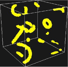
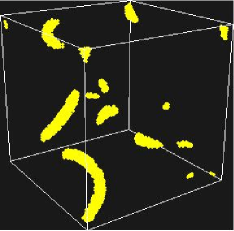
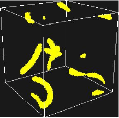
Figure 4: Plot of the magnetic field strength for the semilocal case at $t=40$ (top figures) and at $t=56$ (bottom figures), using the same initial conditions, but evolving the system using a naïve discretization (left) and a lattice link variable discretization (right), as explained in the appendix. Both simulation schemes are in very good agreement, with slightly longer strings in the lattice variable discretization scheme.

Appendix A Discretization methods

In this work, we discretized the equations of motion eq. (5) replacing all the scalar and gauge fields by their values at the lattice points. For instance, a $\mathop{\rm{}U}(1)$ covariant derivative was substituted by

$$D_{j}\phi(x)=\frac{\phi(x+x_{j})-\phi(x-x_{j})}{2L}-\frac{ig_{{\rm{\scriptscriptstyle Y}}}}{2}Y_{i}(x)\phi(x)$$ (12)

where $L$ is the lattice spacing.

It is well known that this discretization scheme does not respect gauge invariance. Nevertheless, we are dealing with well-defined classical equations of motion in a particular gauge, and the breaking of gauge invariance should be irrelevant in this context. Indeed, we make use of the fact that Gauss’s Law is not automatically satisfied, and by monitoring it during the evolution we can check that our discretization is reasonably accurate. This discretization was chosen to facilitate comparison with earlier work [14].

There is an alternative discretization method widely used in the literature which protects gauge invariance and recovers the original equations of motion in the limit where the lattice spacing goes to zero [17]. This method uses lattice link variables, i.e., the replacement of gauge fields by matrices living on the links between lattice points. In this case, a $\mathop{\rm{}U}(1)$ covariant derivative will be substituted by

$$D_{j}\phi(x)=\frac{1}{L}\left(e^{-iLY_{j}(x)}\phi(x+x_{j})-\phi(x)\right).$$ (13)

In order to check whether our conclusions still hold using link variables, we first performed a series of simulations in the semilocal case to determine whether the evolution was compatible. Beginning from the same initial conditions, we evolved the system according to each discretization scheme. We observed that the simulations undergo extremely similar evolution on a pointwise basis, as seen in figure 4, though there are modest differences with slightly longer strings on the lattice gauge calculations, occasionally leading to extra connections.

Figure 5: Plot of string lengths in units of string widths (see text) for the naïve discretization (squares) and the lattice link variable formalism (circles). The data are measured at time $t=56$. The error bars are 1 $\sigma$ over 10 simulations.

To quantify this small difference and its impact on our statistical result, we performed a further 120 simulations using both discretizations. To save computing power we simulated our system in the semilocal case (${\rm sin}^{2}{\theta_{{{\rm W}}}}=1$), discretized in $64^{3}$ cubes for different values of $\beta$. We used several different initial conditions, but for each one we let the system evolve using both the naïve discretization of the (lagrangian) equations of motion and the link variable method for discretizing the (hamiltonian) equations of motion. The initial conditions were calculated using the method b) described in the text (section 3), and as in the electroweak simulations performed in this work, we added an ad hoc damping term ($\eta=0.5$). As our interest lies mainly in the late-time behaviour of the dumbbell network, because the smaller cube size forces $t\lesssim 64$, we chose to calculate the total string length at $t=56$ for both cases.

Figure 5 shows the results. We computed the string lengths as explained in section 4, footnote 2, and then added all string lengths for strings longer than five times their length. That final measure is represented in figure 5, which shows clearly that the differences between the schemes are well within the uncertainties. Although performed for only $64^{3}$ cubes, this result should continue to hold for the larger cubes used to derive the main results in the body of this paper. The system simulated in this test is only the semilocal case, not the full electroweak case, but we are convinced that using the lattice link variable method will not alter significantly the results presented in this paper.

References

- [1] T.W.B. Kibble, Topology of cosmic domains and strings, J. Phys. A 9 (1976) 1387.
- [2] A. Vilenkin and E.P.S. Shellard, Cosmic strings and other topological defects, Cambridge University Press, Cambridge, 1994.
- [3] T. Vachaspati and A. Achucarro, Semilocal cosmic strings, Phys. Rev. D 44 (1991) 3067.
- [4] M. Hindmarsh, Existence and stability of semilocal strings, Phys. Rev. Lett. 68 (1992) 1263.
- [5] A. Achúcarro, J. Borrill, and A. R. Liddle, The formation rate of semilocal strings, Phys. Rev. Lett. 82 (1999) 3742.
- [6] Y. Nambu, String-like configurations in the weinberg-salam theory, Nucl. Phys. B 130 (1977) 505.
- [7] T. Vachaspati, Vortex solutions in the weinberg-salam model, Phys. Rev. Lett. 68 (1992) 1977; erratum ibid. 69 (1992) 216.
- [8] A. Achúcarro and T. Vachaspati, Semilocal and electroweak strings, Phys. Rept. 327 (2000) 347.
- [9] H.B. Nielsen and P. Olesen, Vortex-line models for dual strings, Nucl. Phys. B 61 (1973) 45.
- [10] M. James, L. Perivolaropoulos and T. Vachaspati, Detailed stability analysis of electroweak strings, Nucl. Phys. B 395 (1993) 534 [hep-ph/9212301].
- [11] M. Salem and T. Vachaspati, Band structure in classical field theory, Phys. Rev. D 66 (2002) 025003 [hep-th/0203037].
- [12] J. Garriga and X. Montes, Stability of z strings in strong magnetic fields, Phys. Rev. Lett. 75 (1995) 2268 [hep-ph/9505424].
- [13] M. Hindmarsh, in: Proceedings of the NATO workshop on Electroweak physics and the early universe, J. C. Romão, F. Freire eds., Sintra, Portugal, 1994. Series B: Physics vol. 338, Plenum Press, New York, 1994.
- [14] A. Achúcarro, J. Borrill, and A. R. Liddle, Semilocal string formation in two-dimensions, Phys. Rev. D 57 (1998) 3742
- [15] T. Vachaspati, Estimate of the primordial magnetic field helicity, Phys. Rev. Lett. 87 (2001) 251302
- [16] T. Vachaspati, Electroweak string configurations with baryon number, Phys. Rev. Lett. 73 (1994) 373 [hep-ph/9401220]; erratum ibid. 74 (1995) 1258.
- [17] J.B. Kogut and L. Susskind, Hamiltonian formulation of Wilson’s lattice gauge theories, Phys. Rev. D 11 (1975) 395.
- [18] M. Nagasawa and J. Yokoyama, Are nontopological strings produced at the electroweak phase transition?, Phys. Rev. Lett. 77 (1996) 2166 [hep-ph/9608263].
- [19] M.A. Earnshaw and M. James, Stability of two doublet electroweak strings, Phys. Rev. D 48 (1993) 5818 [hep-ph/9308223].
- [20] C. Bachas, B. Rai and T.N. Tomaras, New string excitations in the two-Higgs standard model, Phys. Rev. Lett. 82 (1999) 2443 [hep-ph/9801263].