An effective Lagrangian description of charged Higgs decays $H^{+}\to W^{+}\gamma,\,W^{+}Z$ and $W^{+}h^{0}$

Abstract

Charged Higgs decays are discussed within an effective lagrangian extension of the two-higgs doublet model, assuming new physics appearing in the Higgs sector of this model. Low-energy contraints are used to imposse bounds on certain dimension–six operators that describe the modified charged Higgs interactions. These bounds are used then to study the decays $H^{+}\to W^{+}\gamma,\,W^{+}Z$ and $W^{+}h^{0}$, which can have branching ratios (BR) of order $10^{-5}$, $10^{-1}$ and $O(1)$, respectively; these modes are thus sensitive probes of the symmetries of the Higgs sector that could be tested at future colliders.

, ,

1.- Introduction. The scalar spectrum of many well motivated extensions of the Standard Model (SM) include a charged Higgs state, whose detection at future colliders would constitute a clear evidence of a Higgs sector beyond the minimal SM. In particular, the two-Higgs doublet model (THDM) has been extensively studied as a prototype of a non-minimal Higgs sector that includes a charged Higgs boson ($H^{\pm}$) [1]. However, a definite test of the mechanism of electroweak symmetry breaking will require further studies of the complete Higgs spectrum. In particular, probing the properties of charged Higgs could help to find out whether it is indeed associated with a weakly-interacting theory, as in the case of the popular minimal SUSY extension of the SM (MSSM) [2], or to an strongly interacting scenario, as in the technicolor models (or its relatives top-color and top-condensate models) [3]. Furthermore, these tests should also allow to probe the symmetries of the Higgs potential, and to determine whether the charged Higgs belongs to a weak-doublet or to some larger multiplet.

Decays of a charged Higgs boson have been studied in the literature, including the radiative modes into $W^{+}\gamma,W^{+}Z$ [4], but mostly within the context of the THDM, or its MSSM incarnation. Charged Higgs production at hadron colliders was studied long ago [5], and recently more systematic calculations of production process at LHC have been presented [6]. Current bounds on charged Higgs mass can be obtained at Tevatron, by studying the top decay $t\to bH^{+}$, which already eliminates some region of parameter space [7], whereas LEP bounds give approximately $m_{H^{+}}>100$ GeV [8].

The decays $H^{+}\to W^{+}\gamma$ and $H^{+}\to W^{+}Z$ may be quite sensitive to new physics effects since they are loop-predicted within the THDM. Indeed, the $W^{+}\gamma$ mode cannot be induced at tree level in any renormalizable theory due to electromagnetic gauge invariance. In turn, the absence of the $W^{+}Z$ mode at tree–level is a feature of models that include only Higgs doublets; it can be induced at this level only in models with Higgs triplets or higher representations, though it is strongly constrained by the custodial symmetry $SU(2)_{c}$. On the other hand, the decay $H^{+}\to W^{+}h^{0}$ happens to be also suppressed for the THDM, when its parameters resemble the ones of the MSSM, specially for its decoupling limit, i.e. when $m_{A}>>m_{Z}$. Though suppressed, these decay modes deserve special attention because they can give valuable information about the underlying structure of the gauge and scalar sectors. Besides, these modes have a clear signature and could be detected at future Hadron colliders. The decay modes of a relatively light charged Higgs boson, with mass of order of the Fermi scale, will depend on the specific structure of a more fundamental theory that incorporates new heavy fields. In this paper we will perform a general study of these decays in a model–independent manner using the effective Lagrangian technique, which is a well motivated scheme to parametrize the virtual effects of physics beyond a given theory, in our case the THDM. We will assume that the spectrum of physical scalars predicted by the THDM are relatively light ($m<O(1)$ TeV) and thus they can be specified within a linear realization of the electroweak group. This corresponds to the decoupling scenario, where the heavy fields cannot affect dramatically the low energy process, though they may have significant contributions on those couplings that are absent or highly suppressed within the THDM. The effective Lagrangian that we will use in this study is a natural extension of the one given in [9] for the minimal SM, which was extended in [10] to study rare decays of the neutral CP–odd scalar predicted by the THDM.

The main goal of this paper is to study the decays of the charged Higgs boson, both within the THDM and its effective Lagragian extension, as possible probes of the Higgs sector. Charged Higgs decays are first discussed within the THDM, which is extended by including higher-dimensional operators. Then, using low-energy data, e.g. the S,T,U parameters, we are able to impose bounds on certain dimension–six operators that also induce modifications to the charged Higgs interactions. We use these bounds to predict the branching ratio for the modes $H^{+}\to W^{+}\gamma,W^{+}Z$ and $W^{+}h^{0}$, which can reach values that could be tested at future colliders.

2.- Decays of the charged Higgs in the THDM. One of the simplest models that predicts a charged Higgs is the THDM, which includes two scalar doublets of equal hypercharge, namely $\Phi_{1}=(\phi^{+}_{1},\phi^{0}_{1})$ and $\Phi_{2}=(\phi^{+}_{2},\phi^{0}_{2})$. This is related to the Higgs content used in the minimal SUSY extension of the SM (MSSM). Besides the charged Higgs ($H^{\pm}$), the spectrum that arises in the THDM includes two neutral CP-even states ($h^{0},H^{0}$, with $m_{h}<m_{H}$), as well as a neutral CP-odd state ($A^{0}$). The most general Higgs potential that includes a softly-broken discrete symmetry $\Phi_{1}\to\Phi_{1}$ and $\Phi_{2}\to-\Phi_{2}$, is given by:

$$V(\Phi_{1},\Phi_{2}) = \mu_{1}^{2}\Phi_{1}^{{\dagger}}\Phi_{1}+\mu_{2}^{2}\Phi_{2}^{{\dagger}}\Phi_{2}-(\mu_{12}^{2}\Phi_{1}^{{\dagger}}\Phi_{2}+h.c.)+\lambda_{1}(\Phi_{1}^{{\dagger}}\Phi_{1})^{2}$$ (1)

$$+ \lambda_{2}(\Phi_{2}^{{\dagger}}\Phi_{2})^{2}+\lambda_{3}(\Phi_{1}^{{\dagger}}\Phi_{1})(\Phi_{2}^{{\dagger}}\Phi_{2})+\lambda_{4}(\Phi_{1}^{{\dagger}}\Phi_{2})(\Phi_{2}^{{\dagger}}\Phi_{1})$$

$$+ \frac{1}{2}[\lambda_{5}(\Phi_{1}^{{\dagger}}\Phi_{2})^{2}+h.c]$$

Diagonalization of the resulting mass matrices gives the expression for the charged Higgs mass-eigenstate: $H^{+}=\cos\beta\phi^{+}_{1}+\sin\beta\phi^{+}_{2}$, where $\tan\beta(=v_{2}/v_{1})$ denotes the ratio of v.e.v.’s from each doublet. The charged Higgs mass is given by:

$$m^{2}_{H^{\pm}}=m^{2}_{A}+\frac{2m^{2}_{W}}{g^{2}}(\lambda_{5}-\lambda_{4})$$ (2)

When $\lambda_{5}=\lambda_{4}$ we have $m_{H^{+}}=m_{A}$, which reflects the underlying custodial symmetry of the Higgs potential.

The predictions for the charged Higgs decays that arise within the THDM and beyond, can be interpreted as possible probes of the symmetries of the Higgs sector. For instance, if we focus on the gauge interactions of the charged Higgs, then the coupling $H^{+}W^{-}h^{0}$ is quite sensitive to the structure of the covariant derivative, and could be one place where to look for deviations from the minimal THDM (or SUSY) predictions. This vertex could induce the decay $H^{+}\to W^{+}h^{0}$, whenever it is kinematically allowed; the corresponding decay width is given by:

$$\Gamma(H^{+}\to W^{+}h^{0}) = \frac{g^{2}\lambda^{\frac{1}{2}}(m^{2}_{H^{\pm}},m^{2}_{w},m^{2}_{h^{o}})}{64\pi m^{3}_{H^{\pm}}}c^{2}_{\beta-\alpha}$$ (3)

$$\times \left[m_{w}^{2}-2(m_{H^{\pm}}^{2}+m^{2}_{h^{o}})+\frac{(m_{H^{\pm}}^{2}-m^{2}_{h^{o}})^{2}}{m^{2}_{w}}\right]$$

where $\lambda$ is the usual kinematic factor, $\lambda(a,b,c)=(a-b-c)^{2}-4bc$. This decay mode has been studied in the literature [11], where it is concluded that its detection at the coming large hadron collider (LHC) is feasible. Within the THDM this decay is proportional to the factor $c_{\beta-\alpha}^{2}$, which will determine the strength of this decay. For instance, within the MSSM, $c_{\beta-\alpha}^{2}\sim m_{z}^{2}/m_{A^{o}}^{2}$, which tends to be small for large values of $m_{A}$, except for small regions of parameter space. Although the BR for this mode can be small in the THDM, new physics could enhance it.

Within the THDM, and other models which treat the charged Higgs as an elementary field, the decay $H^{+}\to W^{+}\gamma$ only arises at the loop level, and tends to has a very small BR (typically smaller than about $10^{-5}$), which could be considered as a generic feature of an elementary Higgs. However, when $H^{+}$ arises from a composite model, the corresponding BR could be enhanced and reach detectable levels [12]. Similarly, the decay $H^{+}\to W^{+}Z$ arises at the loop-level in the THDM, but now for some regions of parameters it could have a large BR, which is a remnant of non-decoupling effects present in the model. On the other hand, in models with Higgs triplets, the decay $H^{+}\to W^{+}Z$ can arise at tree-level, as a result of violations of the custodial symmetry, which is related to the observed value $\rho\simeq 1$. Thus $H^{+}\to W^{+}Z$ can also be used to study the symmetries of the Higgs sector.

Other relevant decays of the charged Higgs boson are the modes into fermion pairs, which include the decays $H^{+}\to\tau\nu_{\tau},c\bar{b}$, and possibly into $t\bar{b}$. If the charged Higgs is indeed associated with the Higgs mechanism, its couplings to fermions should come from the Yukawa sector, and the corresponding decays should have a larger BR for the modes involving the heavier fermions. A very simple test of this could be done through a comparison of the modes $H^{+}\to\tau\nu_{\tau}$ and $H^{+}\to\mu\nu_{\mu}$, which should be quite different if the charged Higgs comes as a remmant of the Higgs mechanism.

In order to discuss the new results of the following section, and to present our notation and conventions, we found convenient to discuss here the loop-decays of the charged Higgs in the THDM. Although these decays have been partially discussed in the literature, we have also opted to perform our own calculation to verify previous results, for which we find complete agreement. We have evaluated the corresponding amplitudes for both $H^{+}\to W^{+}\gamma$ and $H^{+}\to W^{+}Z$, using dimensional regularization, with the help of the programs Feyncalc [13] and the numerical package FF  [14]. We shall not present here all the detailed analytical expressions for the amplitudes, which are obtained using the non-linear gauge, as described previously in ref.[15]; instead only their generic form will be displayed. The complete list of diagrams encountered in the calculation, and the full expressions for the results will be presented elsewhere [16] .

Using a non-linear gauge eliminates the three-point vertices of the type $WVG$ (where $V$ represents the neutral gauge bosons, and $G$ denotes the charged Goldstone boson), which reduces considerably the number of diagrams, this helps to simplify the calculation and to verify the gauge invariance in the case of the $W\gamma$ mode. Our result for the total amplitude of the decay $H^{+}\to W^{+}V$ (with $V=\gamma,Z$) can be summarized as:

$$\mathcal{M}_{V}=-\frac{ig}{m_{W}}\epsilon^{\mu}\epsilon^{\nu}\bigg{[}m^{2}_{W}F_{V}g_{\mu\nu}+G_{V}k_{1\mu}k_{2\nu}\\ +iH_{V}\epsilon_{\mu\nu\alpha\beta}k^{\alpha}_{1}k^{\beta}_{2}\bigg{]},$$

where $F_{V},G_{V},H_{V}$ denote the contributions from the loop graphs to the amplitudes, and $\epsilon^{\mu}(k_{1},\lambda_{1})$ and $\epsilon^{\nu}(k_{2},\lambda_{2})$ represent the polarization vectors of the $W$ and $V$ gauge bosons, respectively.

For the mode $H^{+}\to W^{+}\gamma$ we have: $m^{2}_{W}F_{V}=-G_{V}k_{1}.k_{2}$, and then the corresponding decay width is given by:

$$\Gamma(H^{+}\to W^{+}\gamma)=\frac{g^{2}m^{3}_{H^{+}}}{32\pi m^{2}_{W}}\lambda^{3/2}(1,w,0)[|G_{\gamma}|^{2}+|H_{\gamma}|^{2}]$$ (4)

where $\lambda(x,w,z)=(x-w-z)^{2}-4wz$, and $w=m^{2}_{W}/m^{2}_{H^{+}}$, $z=0$.

On the other hand, the decay width for the mode $H^{+}\to W^{+}Z$ is conveniently written as:

$$\Gamma(H^{+}\to W^{+}Z)=\frac{m_{H^{+}}}{16\pi}\lambda^{1/2}(1,w,z)[|V_{TT}|^{2}+|V_{LL}|^{2}]$$ (5)

where here $w=m^{2}_{W}/m^{2}_{H^{+}}$, $z=m^{2}_{Z}/m^{2}_{H^{+}}$ and the quantities $|V_{TT}|^{2}$ and $|V_{LL}|^{2}$ are the separate contributions of the longitudinaly and transversely polarized final W- and Z-bosons. They are explicitly given by

$$|V_{LL}|^{2} = \frac{g^{2}}{4z}\left|(1-w-z)F_{Z}+\frac{\lambda(1,w,z)}{2w}G_{Z}\right|^{2}$$ (6)

$$|V_{TT}|^{2} = g^{2}\left[2w|F_{Z}|^{2}+\frac{\lambda(1,w,z)}{2w}|H_{Z}|^{2}\right]$$

To evaluate the branching ratios we have used the expressions for the decay widths of the tree-level modes, as appearing in ref. [1]. We have taken $m_{t}=175\;$ GeV, and the values for the electroweak parameters of the table of particle properties [17]. We shall present the resulting BR for the charged Higgs decays in Figs. 1-3 of the following sections. For the moment we only mention the BR for these decays for the following three relevant scenarios, which assume $m_{h}=115$ GeV,

a) SUSY-like scenario. Here we assume an approximately degenerated spectrum of heavy Higgs bosons, i.e. $m_{H^{+}}\simeq m_{H}\simeq m_{A}$, and also $\alpha\simeq\beta-\pi/2$. In this case the BR for the mode $W^{+}h^{0}$ is about $2\times 10^{-2}$ ($7\times 10^{-5}$) for $m_{H^{+}}=300$ GeV and $\tan\beta=7$ (30). On the other hand, the BR for the mode $H^{+}\to W^{+}Z$ is about $10^{-3}$ ($3\times 10^{-5}$), whereas for $H^{+}\to W^{+}\gamma$ is about $2\times 10^{-6}$ ($10^{-7}$) for the same values of parameters. In this scenario $H^{+}\to W^{+}h^{0}$ and $H^{+}\to W^{+}Z$ have similar BR’s.

b) Non-decoupling scenario-A. Now we take a large mass difference between $A^{0}$ and $H^{+}$, i.e. $m_{H^{+}}-m_{A}=300$ GeV, with $m_{H}\simeq m_{H^{+}}$, and also $\alpha\simeq\beta-\pi/2$. In this case we find that the mode $W^{+}h^{0}$ has a BR about $10^{-3}$ ($2\times 10^{-5}$), for $m_{H^{+}}=300$ GeV and $\tan\beta=7$ (30). Similarly, the BR for the mode $H^{+}\to W^{+}Z$ is about $4\times 10^{-2}$ ($4\times 10^{-3}$), whereas the BR for $H^{+}\to W^{+}\gamma$ is about $2\times 10^{-6}$ ($2\times 10^{-7}$), for the same values of parameters. In this case, $H^{+}\to W^{+}Z$ dominates.

c) Non-decoupling scenario-B. Here we also assume a large mass difference between $A^{0}$ and $H^{+}$, i.e. $m_{A}-m_{H^{+}}=300$ GeV, with $m_{H}\simeq m_{H^{+}}$, but now with $\alpha\simeq\beta-\pi/4$. In this case we find that the BR for the mode $W^{+}h^{0}$ has a BR about $1$ ($0.2$) for $m_{H^{+}}=300$ GeV and $\tan\beta=7$ (30). Similarly, the BR for the mode $H^{+}\to W^{+}Z$ is about $10^{-2}$ ($4\times 10^{-3}$), whereas the BR for $H^{+}\to W^{+}\gamma$ is about $4\times 10^{-7}$ ($2\times 10^{-7}$), for the same values of parameters. In this scenario $H^{+}\to W^{+}h^{0}$ clearly dominates, even above the $t\bar{b}$ mode.

3.- Charged Higgs decays in the effective Lagragian approach. The relevant operators needed for an effective lagrangian description of the THDM were previously studied in ref.[10]. Here we show those operators of the lower dimension that could potentially induce corrections to the charged Higgs vertices. The corresponding effective Lagrangian has the following form:

$$\mathcal{L}_{eff}=\mathcal{L}_{THDM}+\sum_{n\geq 6}\bigg{[}\sum_{i}\frac{\alpha^{i}_{n}}{\Lambda^{n-4}}(\mathcal{O}^{i}_{n}+h.c.)\bigg{]}$$ (7)

where $\mathcal{L}_{THDM}$ is the THDM Lagrangian, $\Lambda$ is the new physics scale, $\mathcal{O}^{i}_{n}$ are higher–dimension $SU(2)\times U_{Y}(1)$ invariant operators, and $\alpha^{i}_{n}$ are unknown parameters, whose order of magnitude can be estimated because gauge invariance makes possible to establish the order of perturbation theory at which each operator can be generated in the fundamental theory [18]. This fact allows to introduce a hierarchy among the operators of a given dimensionality, which has important consequences from the practical point of view, since the operators generated at loop levels would be suppressed by the loop factor $(4\pi)^{-2}$ with respect to those induced at tree level. In the following we shall consider only the lower dimension operators, namely, those of dimension–six that may be generated at tree level in the fundamental theory. It will be seen below, after SSB some of these operators introduce modifications to the quadratic terms of the dimension–four theory, so a redefinition of fields and parameters will be needed in order to obtain the canonical form for the propagators. We shall classify the operators that modify the charged Higgs vertices, and could potentially induce corrections to the charged Higgs decays $H^{+}\to W^{+}V$ and $H^{+}\to W^{+}h^{o}$, as follows:

i) Operators that contain only scalar fields. These operators modify the Higgs potential and the kinetic structure of the scalar fields, and are given by:

$$\mathcal{O}^{\phi}_{ijklmn} = \frac{1}{3}(\Phi_{i}^{{\dagger}}\Phi_{j})(\Phi_{k}^{{\dagger}}\Phi_{l})(\Phi_{m}^{{\dagger}}\Phi_{n})$$ (8)

$$\mathcal{O}^{\partial\phi}_{ijkl} = \frac{1}{2}\partial_{\mu}(\Phi_{i}^{{\dagger}}\Phi_{j})\partial^{\mu}(\Phi_{k}^{{\dagger}}\Phi_{l})$$ (9)

where $i,j,k,l,m,n=1,2$ and $\Phi_{i}$ is a Higgs doublet. There are several operators, depending on the possible combinations $i,j,k,l$ of the two doublets, but for our purpose, it is sufficient to consider only those that satisfy the discrete symmetry $\Phi_{1}\to\Phi_{1}$ and $\Phi_{2}\to-\Phi_{2}$. This symmetry allows only eight operators of the type (8), from which the combinations $(111212),(221212),(111221)$, and $(221221)$ do not respect the custodial symmetry. On the other hand, there are five operators of the type (9) and two of them violate the custodial symmetry too, namely those corresponding to the combinations $(1221)$ and $(1212)$.

When the operators (9) are included in the Higgs potential, they will induce modifications to the minimization conditions, and the angle $\alpha$ (but not $\beta$) need to be redefined. This redefinition can be worked out to the first order in the parameters $\alpha^{i}$. Moreover, the operators (9,10), when included in the Higgs sector of model, will modify the Feynman rules for the scalar couplings, and will induce new contributions to the loop-amplitude for the decay $H^{+}\to W^{+}\gamma$ through the vertices $H^{+}H^{-}\phi$. These operators also affect the mass relations of the physical Higgs states as follows

$$m_{\phi}^{2}=m_{\phi}^{\circ 2}(1+\sum_{i}\epsilon^{i}_{\phi})$$ (10)

where $\phi=H^{+},H^{o},h^{o},A^{o}$ and the parameters $\epsilon_{\phi}^{i}$ are functions of the ratio of energy scales $(v/\Lambda)^{2}$ and the parameters $\alpha^{i}$, associated with the contributions from the operators $\mathcal{O}^{i}$ (in what follows, it will be understood that the coefficient $\epsilon$ contain the multiplicative factor $(v/\Lambda)^{2}$). $m^{\circ}_{\phi}$ denotes the mass of the $\phi$ state within THDM, i.e., the superscript $\circ$ denotes mass relations arising from the dimension–four theory.

ii) Operators that modify the Higgs-gauge boson interactions. This set includes the following,

$$\mathcal{O}_{ijkl}^{(1)} = \Phi^{{\dagger}}_{i}\Phi_{j}(D_{\mu}\Phi_{k})^{{\dagger}}(D^{\mu}\Phi_{l})$$ (11)

$$\mathcal{O}_{ijkl}^{(2)} = \left[\Phi^{{\dagger}}_{i}(D_{\mu}\Phi_{j})\right]\left[(D_{\mu}\Phi_{k})^{{\dagger}}\Phi_{l}\right]$$ (12)

There are six operators of each type, consistent with the discrete symmetry $\Phi_{1}\to\Phi_{1},\Phi_{2}\to-\Phi_{2}$. While all six operators of the type (12) violate the custodial symmetry, the ones of the type (11) do respect it. In fact, these operators lead to a redefinition of the gauge boson masses given by

$$m^{2}_{W} = m^{\circ 2}_{W}(1+\epsilon^{(1)}_{z}),$$ (13)

$$m_{Z}^{2} = m^{\circ 2}_{Z}(1+\epsilon^{(1)}_{z}+\epsilon^{(2)}_{z}),$$ (14)

where $\epsilon^{(1)}_{z}$ and $\epsilon^{(2)}_{z}$ are the modifications introduced by the operators (11) and (12) to the gauge boson masses, respectively, which imply the constraint

$$\Delta\rho=|\epsilon_{z}^{(2)}|\leq 0.003$$ (15)

This shows that operators (12) do not respect the custodial symmetry, which automatically guarantee the existence of the $H^{+}W^{-}Z$ vertex, but this will be suppressed by the $\rho$ parameter. However, it is important to notice that both operators (12) and (11) induce the $H^{+}W^{-}Z$ vertex, so the effective Lagrangian approach tells us that this interaction can be directly induced by operators that respect the custodial symmetry, whose contributions to this vertex may be dominant since they are generated at tree level in the fundamental theory. Thus, we can study the decay $H^{+}\to W^{+}Z$ considering only the vertex contributions arising from the set of operators (11,12), including as well the loop prediction of the THDM. On the other hand, the contribution of this vertex to the decay $H^{+}\to W^{+}\gamma$ should also be considered since it is a loop contribution in the context of the full theory.

Moreover, the operators (8,9,11,12) modify the prediction of the dimension–four theory for the relation between the masses of the charged and the neutral CP–odd Higgs, as follows

$$m_{H^{\pm}}^{2}=m_{A^{o}}^{2}+\frac{2m_{W}^{2}}{g^{2}}\bigg{[}(1-\epsilon^{(1)})(\lambda_{5}-\lambda_{4})-\epsilon_{AH}^{\phi}+\frac{g^{2}m_{A^{o}}^{2}}{2m_{W}^{2}}(\epsilon_{A^{o}}^{\partial\phi}+\epsilon_{A^{o}}^{(2)})\bigg{]},$$ (16)

where $\epsilon^{(1)}$ denote a combination of the coefficients of the operators (11), $\epsilon_{AH}^{\phi}$ are contributions of the operators (8), which violate the custodial symmetry. $\epsilon^{\partial\phi}_{A^{0}}$ and $\epsilon^{(2)}_{A^{0}}$ are functions of the coefficients of the operators (9) and (12), respectively, which do not respect the custodial symmetry neither. When $\lambda_{4}=\lambda_{5}$ and $\epsilon_{A^{o}}^{\partial\phi},\epsilon^{(2)}_{A^{0}},\epsilon_{AH}^{\phi}\to 0$ , we have $m_{H^{\pm}}=m_{A^{o}}$, and the custodial symmetry of the Higgs potential is recovered.

iii) Yukawa-like operators. This set will involve the fermion fields, but here we shall not consider fermion mixing and will keep only the expressions for the 3rd family quarks, which dominates the fermionic contribution to the loop amplitudes in $H^{+}\to W^{+}\gamma$. We include,

$$\mathcal{O}_{ijk}^{t\phi} = \Phi_{i}^{\dagger}\Phi_{j}\bar{Q}_{L}\tilde{\Phi}_{k}t_{R}$$ (17)

$$\mathcal{O}_{ijk}^{b\phi} = \Phi_{i}^{\dagger}\Phi_{j}\bar{Q}_{L}\Phi_{k}b_{R},$$ (18)

where $Q_{L}=(t,b)_{L}$ is the left–handed $SU_{L}(2)$ doublet. After SSB, these operators introduce modifications into the fermion masses and also effective interactions of dimension four among the charged Higgs and the members of the 3rd family quarks. Thus, they contribute to $H^{+}\to W^{+}\gamma$ through the $H^{+}tb$ vertex. Since this vertex has a renormalizable structure, its contribution will be finite.

iv) Operators that will induce corrections to the charged and neutral currents of the SM. Here we consider the following operators,

$$O_{ij}^{\phi Q(1)} = i(\Phi^{{\dagger}}_{i}D_{\mu}\Phi_{j})\bar{Q}_{L}\gamma^{\mu}Q_{L}$$ (19)

$$O_{ij}^{\phi Q(2)} = i(\Phi^{{\dagger}}_{i}D_{\mu}\tau^{a}\Phi_{j})\bar{Q}_{L}\gamma^{\mu}\tau^{a}Q_{L}$$ (20)

$$O_{ij}^{\phi t} = i(\Phi^{{\dagger}}_{i}D_{\mu}\Phi_{j})\bar{t}_{R}\gamma^{\mu}t_{R}$$ (21)

$$O_{ij}^{\phi b} = i(\Phi^{{\dagger}}_{i}D_{\mu}\Phi_{j})\bar{b}_{R}\gamma^{\mu}b_{R}$$ (22)

These operators introduce modifications into the dimension–four vertices $H^{+}tb$ and $W^{+}tb$, which contribute to the loop decay $H^{+}\to W^{+}\gamma$. Nonrenormalizable vertices of dimension–five of the type $H^{+}tb\gamma$, $H^{+}W^{-}tt$, and $H^{+}W^{-}bb$ (and also the $H^{+}tb$ one with derivative structure) are also induced from operators (20-23). These dimension–five vertices lead to a divergent contribution to the loop-amplitude for the decay $H^{+}\to W^{+}\gamma$, which we have renormalized using the $\overline{MS}$ scheme [19]. This set of operators has the advantage that can be bounded by their contributions to the S,T,U parameters, through the decay $\Gamma(Z\to\bar{b}b)$ [20]. Working at tree–level, as it was done in ref.[21] for the analogous contribution of the effective operators of the minimal SM to the S, U, T parameters, we derive an order of magnitude bound, $\epsilon_{i}\leq O(10^{-3})$, which we will assume hereafter for the coefficients of all operators.

Now we can discuss the effect of these operators on the charged Higgs interactions. In order to probe these effects one can first study the corrections to the decay width for $H^{+}\to W^{+}h^{o}$; the result is given now as follows:

$$\Gamma(H^{+}\to W^{+}h^{0})=\Gamma_{\tiny THDM}(H^{+}\to W^{+}h^{0})\left[1+\frac{\epsilon^{(1)}_{HWh}+\epsilon^{(2)}_{HWh}}{c_{\beta-\alpha}}\right]^{2}$$ (23)

where $\Gamma_{\tiny THDM}(H^{+}\to W^{+}h^{0})$ is given in eq.(3) and $\epsilon^{(1),(2)}_{HWh}$ includes effects from operators (11,12). Since the operators (12) are highly constrained by the custodial symmetry, this decay would be dominated by the contributions arising from operators (11).

Regarding the decay $H^{+}\to W^{+}Z$, we shall only consider the operators (11,12), which induce effectively this vertex. The resulting effective amplitude will be added to the loop result obtained in the previous section. The new form can be obtained simply by replacing: $F_{Z}\to F_{Z}+\Delta F_{Z}$, $G_{Z}\to G_{Z}+\Delta G_{Z}$ and $H_{Z}\to H_{Z}+\Delta H_{Z}$, with: $\Delta F_{Z}=\frac{S_{eff}}{c_{w}}$, $\Delta G_{Z}=\Delta H_{Z}=0$, and $S_{eff}=s_{w}^{2}\epsilon_{HWZ}^{(1)}+\epsilon^{(2)}_{HWZ}$. The parameters $\epsilon^{(1,2)}_{HWZ}$ are functions of coefficients that come from the operators (11,12). The operators (12) are associated with the breaking of the custodial symmetry in the Higgs sector, and the decay $H^{+}\to W^{+}Z$ will be sensitive to its strength.

Finally, for the decay $H^{+}\to W^{+}\gamma$ we shall consider the one-loop contribution induced by the tree–level–generated dimension–six operators listed in the paragraphs i), ii), iii), iv); the operators of iv) have the convenience of being constrained by the S,T,U parameters. We have performed the loop calculation using a nonlinear gauge–fixing procedure. This scheme is suited to eliminate vertices of the type $WVG$ involving the Goldstone bosons, not only from the renormalizable Lagrangian but also from the effective operators (12) that introduce modifications to the unphysical vertex $WZG_{W}$. We have introduced the following nonlinear gauge–fixing functions which transform covariantly under the $U_{e}(1)$ group:

$$f^{+} = \left[D^{e}_{\mu}+\frac{igs^{2}_{w}}{c_{w}}\bigg{(}1+\frac{\epsilon^{(2)}_{z}}{s^{2}_{w}}\bigg{)}Z_{\mu}\right]W^{+\mu}-i\xi m_{W}G_{W}^{+},$$

$$f^{Z} = \partial_{\mu}Z^{\mu}-\xi m_{Z}G_{Z}^{o},$$ (24)

$$f^{A} = \partial_{\mu}A^{\mu},$$

where $D^{e}_{\mu}$ is the electromagnetic covariant derivative and $\xi$ is the gauge parameter. The Feynman Rules for vertices of the type $WWZ$ are modified too, and are consistently used to obtain the loop amplitude (the full list of Feynman rules in this gauge as well as the corresponding graphs for the radiative decays will appear elsewhere [16] ).

At one–loop level in the full theory, the decay $H^{+}\to W^{+}\gamma$ also receives a direct contributions from loop–generated dimension–six operators. These operators are

$$\mathcal{O}_{ij} = (\Phi^{\dagger}_{i}{\bf W}_{\mu\nu}\Phi_{j})B^{\mu\nu},$$ (25)

$$\widetilde{\mathcal{O}}_{ij} = (\Phi^{\dagger}_{i}{\bf W}_{\mu\nu}\Phi_{j})\widetilde{B}^{\mu\nu},$$ (26)

where ${\bf W}_{\mu\nu}=\tau^{a}W_{\mu\nu}$ and $\widetilde{B}_{\mu\nu}=\frac{1}{2}\epsilon_{\mu\nu\lambda\rho}B^{\lambda\rho}$. In the calculation of this decay we have explicitly introduced the loop factor $(4\pi)^{-2}$ in the coefficients of these operators.

Finally, the expressions for the decay width of $H^{+}\to W^{+}\gamma$ can be written as in eq.(5), by making the substitutions, $G_{\gamma}\to G_{\gamma}+\Delta G_{\gamma}$ and $H_{\gamma}\to H_{\gamma}+\Delta H_{\gamma}$. Besides the amplitudes induced by the above loop–generated operators, the terms $\Delta G_{\gamma}$ and $\Delta H_{\gamma}$ contain the loop contributions coming from the tree–level–generated operators given in paragraphs i), ii), iii), iv). The result depends on Passarino–Veltman scalar two– and three–point functions, and due to the presence of nonrenormalizables vertices induced by the operators of iv), the divergent parts of some two–point functions do not disappear, so a renormalization scheme must be adopted. We used the $\overline{MS}$ scheme with the renormalization scale specified by $\mu=\Lambda$, which leads to a logarithmic dependence in the corresponding amplitudes of the form $ln(m^{2}_{i}/\Lambda^{2})$, $m_{i}$ being one of the masses circulating in the loops. In order to evaluate these logarithms, we have estimated the value of $\Lambda$ using the bounds obtained from the S, T, U parameters. The expressions for these contributions are very long too and will be presented elsewhere [16].

In the description of physics beyond the Fermi scale that we are using, the corrections coming from the higher-dimensional operators can represent new physics of perturbative type, e.g. SUSY particles, new fermions, etc, whose coefficients will be typically small ($\alpha_{i}\approx 0.1-1$). Assuming that new physics would be apparent at scales of order $\Lambda\approx 1$ TeV, a typical tree–level–generated dimension–six operator will have a suppression factor within the range $(v/\Lambda)^{2}\alpha_{i}\approx 10^{-2}-10^{-1}$. However, in order to make predictions, we have adopted a more conservative point of view by choosing values for the coefficients of the various operators of order $10^{-3}$, similar to the bounds determined for the operators that are constrained by the S, T, U parameters. The numerical results are shown in Figs.1,2,3. We comment here on the changes induced by the effective operators for the charged Higgs branching ratios, of the three scenarios discussed in the THDM section, taking the same values of parameters that define each case, namely

a) SUSY-like scenario. For $tan\beta=7$, the BR for the mode $W^{+}h^{0}$ goes from $10^{-2}$ (THDM) up to $2\times 10^{-2}$ (Eff. Lagrangian); whereas the BR for the mode $H^{+}\to W^{+}Z$ goes from $10^{-3}$ (THDM) to $7\times 10^{-3}$(Eff. Lagrangian), and $H^{+}\to W^{+}\gamma$ goes from $2\times 10^{-6}$ (THDM) up to $10^{-5}$ (Effective Lagrangian), which is the mode with largest enhancement for this scenario.

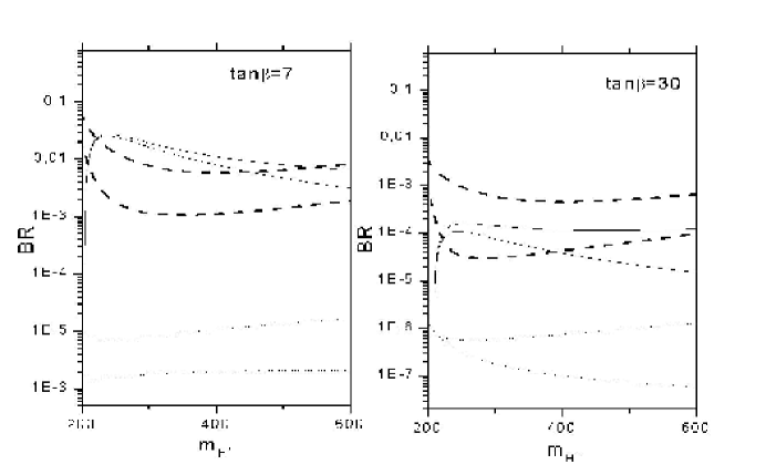
Figure 1: Branching ratios for charged Higgs decay into $Wh$ (solid), $WZ$ (dashes) and $W\gamma$ (dots) for the parameters, $m_{h}=115$ GeV, $m_{H^{\pm}}\simeq m_{A}\simeq m_{H}$ and $\alpha\simeq\beta-\pi/2$. Lower (upper) lines correspond to the THDM (effective Lagrangian) cases.

b) Non-decoupling scenario-A. In this case, for $\tan\beta=7$ again, the BR for the mode $W^{+}h^{0}$ goes from $10^{-3}$ (THDM) up to $2\times 10^{-3}$ (Eff. Lagrangian); whereas the BR for the mode $H^{+}\to W^{+}Z$ goes from $4\times 10^{-2}$ (THDM) to $10^{-1}$(Effective Lagrangian), and $H^{+}\to W^{+}\gamma$ goes from $2\times 10^{-6}$ (THDM) up to $10^{-5}$ (Effective Lagrangian).

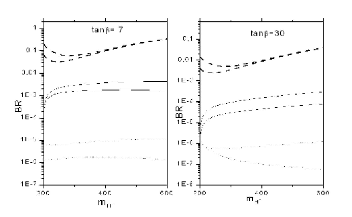
Figure 2: Same as in fig. 1, but now with parameters $m_{H^{\pm}}-m_{A}=300$ Gev, $m_{H}\simeq m_{H^{\pm}}$ and $\alpha\simeq\beta-\pi/2$.

c) Non-decoupling scenario-B. For $\tan\beta=7$, the BR for the mode $W^{+}h^{0}$ remmains approximately constant for both the THDM and the Eff. Lagrangian; whereas the BR for the mode $H^{+}\to W^{+}Z$ goes from $10^{-2}$ (THDM) to $2\times 10^{-2}$(Effective Lagrangian), and $H^{+}\to W^{+}\gamma$ goes from $3\times 10^{-7}$ (THDM) up to $10^{-6}$ (Eff. Lagrangian).

Results for $\tan\beta=30$ show a similar behaviour for all previous cases.

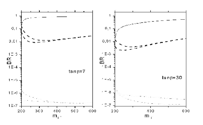
Figure 3: Same as in fig. 1, but now with parameters $m_{H^{\pm}}-m_{A}=300$ Gev, $m_{H}\simeq m_{H^{\pm}}$ and $\alpha\simeq\beta-\pi/4$.

4.- Conclusions. We have studied the rare decays of the charged Higgs boson $H^{+}\to W^{+}h^{o},W^{+}Z,W^{+}\gamma$ as possible tests of the symmetries of the Higgs sector. Starting from the two-higgs doublet model, where the radiative decays are in general suppressed, we construct an effective Lagrangian extension of the model, that describes the modified charged Higgs interactions. The S,T,U parameters are used to impose bounds on certain dimension–six operators that describe some of these interactions, and used to make predictions on the decays $H^{+}\to W^{+}\gamma,W^{+}Z,W^{+}h^{0}$. We find that theses modes can receive an enhancement that could be tested at future colliders. For the discussion of results we have identified three scenarios, whose characteristics can be tested at future colliders, as they lead to different predictions for these modes, namely: a) a SUSY-like case, where the modes $WZ$ and $Wh$ have similar BR, b) a non-decoupling scenario, with parameters leading the $WZ$ mode to become the dominant one, and c) a non-decoupling case where the mode $Wh$ becomes the dominant one. As we can see from Figures 1–3, there is a large enhancement for the modes $W^{+}\gamma$ and $W^{+}Z$, when passing from the THDM to the effective Lagrangian framework, whereas the mode $W^{+}h^{0}$ receives a moderate enhancement.

Acknowledgments. We acknowledge financial support from CONACYT and SNI (México). Fruitful discussions with J. M. Hernández and M.A. Pérez are also acknowledged.

References

- [1] S. Dawson et al., The Higgs Hunter’s Guide, 2nd ed., Frontiers in Physics Vol. 80 (Addison-Wesley, Reading MA, 1990).
- [2] M. Carena et al., Report of the Tevatron Higgs working group; FERMILAB-CONF-00-279-T; hep-ph/0010338; see also: C. Balazs et al., Phys. Rev. D59 (1999) 055016; J.L. Diaz-Cruz et al., Phys. Rev, Lett. 80 (1998) 4641.
- [3] See for instance: B. Dobrescu, Phys. Rev. D63 (2001) 015004.
- [4] J.L. Diaz-Cruz and M.A. Pérez, Phys. D33 (1986) 273 ; J. Gunion, G. Kane and J. Wudka, Nucl. Phys. B299 (1988) 231; A. Mendez and A. Pomarol, Nucl. Phys. B349 (1991) 369; E. Barradas et al., Phys. Rev. D53 (1996) 1678; M. Capdequi Peyranere, H. E. Haber, and P. Irulegui, Phys. Rev. D44 (1991) 191; S. Kanemura, Phys. Rev. D61 (2000) 095001.
- [5] J.L. Diaz-Cruz and O.A. Sampayo, Phys. Rev. D50 (1994) 6820; J. Gunion et al., Nucl. Phys. B294 (1987) 621; M. A. Pérez and A. Rosado, Phys. Rev. D30 (1984) 228.
- [6] M. Bisset et al, Eur. Phys. J. C19 (2001) 143; A. Barrientos Bendezu and B.A. Kniehl, Phys. Rev. D63 (2001) 015009; Zhou Fei et al., Phys. Rev. D63 (2001) 015002; D.J. Miller et al., Phys. Rev. D61 (2000) 055011.
- [7] F. Abe et al. (CDF Collaboration), Phys. Rev. Lett. 79 (1997) 357.
- [8] For a review see: F. Borzumati and A. Djouadi, hep-ph/9806301.
- [9] W. Buchmuller and D. Wyler, Nucl. Phys. B268 (1986) 621.
- [10] M.A. Perez, J. J. Toscano and J. Wudka, Phys. Rev. D52(1995) 494.
- [11] S. Moretti, Phys. Lett. B481 (2000) 49.
- [12] H. Schlereth, preprint PSI-PR-93-03; see also ref. 3.
- [13] R. Mertig, M. Bhom, and A. Denner, Comput. Phys. Commun. 64 (1991) 345.
- [14] G. J. van Oldenborgh and J.A.M. Vermaseren, Zeit. Phys. C46, 425 (1990).
- [15] U. Cotti, J.L. Diaz-Cruz and J.J. Toscano, Phys. Lett. B404 (1997) 308; ibid, Phys. Rev. D62 (2000) 116005.
- [16] J.L. Díaz-Cruz, J. Hernández-Sánchez and J.J. Toscano, work in progress.
- [17] Review of Particle Properties, Eur. Phys. J. C15 (2000) 1.
- [18] C. Arzt, M. B. Einhorn and J. Wudka, Nucl. Phys.B433 (1995) 41.
- [19] C. Arzt, M. B. Einhorn and J. Wudka, Phys. Rev. D49 (1994) 1370; J. Novotny and M. Stohr, Czech. J. Phys. 49 (1999) 1471.
- [20] A. Kundu and P. Roy, Int. J. of Mod. Phys. A12 (1997) 1511.
- [21] G. Sánchez–Colón and J. Wudka, Phys. Lett. B432 (1998) 383.