Schrödinger functional at negative flavour number

Abstract

The scaling of the Schrödinger functional coupling is studied numerically and perturbatively for an SU(3) lattice gauge field coupled to an $O(a)$ improved bosonic spinor field. This corresponds to QCD with minus two light flavours and is used as a numerically less costly test case for real QCD. A suitable algorithm is developed, and the influence of the matter fields on the continuum limit and the lattice artefacts are studied in detail.

1 Introduction

The strong coupling constant $\alpha_{s}$ of QCD is of particular theoretical interest. On the one hand, it can be extracted from jet events which are a property of the strong interaction at large energies. On the other hand, as has been discussed in detail in [1], the running coupling can be computed in lattice gauge theory. There, the parameters may be fixed in the non perturbative hadronic regime, taking as experimental input for example the pion decay constant and the masses of the $\pi,\ K,\ D$ and $B$. The computation of the running of the coupling up to large energies thus provides a quantitative test of the theory, which is believed to be fundamental in the hadronic as well as in the high energy regime. Furthermore, it is interesting to find out at which energies the perturbative behaviour of a given coupling sets in.

The basic strategy for such a computation has been proposed by Lüscher, Weisz and Wolff [2]. They use a non perturbative definition of the coupling, which runs with the spacetime volume. Its evolution is mapped out by a recursive finite size scaling technique up to large energies where contact with the minimal subtraction scheme is made by perturbation theory. The central object in this computation is the step scaling function, which can be understood as a beta function for finite scale transformations. At each step in the recursive evolution of the coupling, the continuum limit is taken. Other key ingredients include ${\rm O}(a)$ improvement and Schrödinger functional boundary conditions [3, 4, 5].

This strategy applies to any asymptotically free theory, and it has first been tested for the nonlinear $O(3)$ model in two dimensions [2], pure $SU(2)$ gauge theory [6], and pure $SU(3)$ gauge theory [7, 8], which can also be interpreted as the quenched approximation of QCD. In [9], the ALPHA collaboration has just published their first quantitative results for the evolution of the coupling in QCD with two flavours.

However, since simulations in full QCD are notorious for high computational cost, the data at $N_{\rm f}=2$ do not yet reach very close to the continuum limit in the individual steps of the computation. Therefore, we have decided to also study the approach to the continuum in a simpler model that is more easily accessible to simulation. It differs from the quenched approximation by depending on the fermionic determinant. In this computation, the focus is not so much on the running coupling as a function of the energy scale, but rather on the details of the approach of the continuum limit in the perturbative regime and at slightly lower energy.

The model we investigate in this paper may be viewed as arising from an analytic continuation of the flavour number to negative values and in particular to $N_{\rm f}=-2$. Since a negative power of the fermionic determinant may be represented by bosonic spinor fields with the same indices as fermionic fields, the name bermions was coined for such theories [10]. The main virtue of these models is that the interaction term becomes local and thus numerical simulations are considerably cheaper than in full QCD.

In the literature (e.g. [11, 10]), they were mainly considered from an algorithmic point of view with the idea in mind to extrapolate in $N_{\rm f}$ from negative values to $N_{\rm f}=2$. However, this is problematical, since fermionic zero modes may be encountered (for example at small quark masses or in large physical volume), which dominate the dynamics in the theories at negative flavour numbers. Thus, in our work, no extrapolation of results from negative to positive values of $N_{\rm f}$ is attempted or aimed at.

In [12], two of the authors have published results for the step scaling function for unimproved Wilson bermions ($N_{\rm f}=-2$) in the perturbative regime. Lattice artefacts turned out to be very large. As for the quenched approximation and for full QCD with two flavours, we now study the ${\rm O}(a)$ improved $N_{\rm f}=-2$ theory. The inclusion of the clover term into the bermionic action poses certain algorithmic problems that are dealt with in this article. We present a detailed study of the performance of the algorithm used for our Monte Carlo simulations.

An important input for the understanding of our Monte Carlo data comes from lattice perturbation theory. The cutoff effects of the step scaling function can be computed perturbatively. They are used in the data analysis. The cutoff effects have already been estimated in [13] to 2-loop order. However, in that calculation, the continuum value of the critical mass has been used as a first estimate instead of the finite lattice value, which was not yet available (see discussion in  [13]). The computation of this critical mass is technically more involved due to extra tadpole diagrams that emerge from the non vanishing background field. Here we present a computation that includes all diagrams and completes the study of [13].

This article is organized in the following way. In the next section, we reflect the most important definitions that occurred in our previous articles. In section 3, we discuss the perturbative expansion of the lattice artefacts of the step scaling function. After that, the bermion model and the algorithm used in our non-perturbative calculations is discussed. In the last section, our numerical results are summarized.

2 Lattice theory

Since this work extends our earlier work reported in [3, 7, 12], we only briefly summarize the necessary notations. For unexplained conventions, we refer in particular to [14, 15].

The theory is set up on a four dimensional hyper-cubic Euclidean lattice with lattice spacing $a$ and size $T\times L^{3},T=L$, $L$ being an integer multiple of $a$. The gauge field on this lattice is represented by an $SU(3)$ matrix $U(x,\mu)$ that is defined on every link between nearest neighbour sites $x$ and $x+a\hat{\mu}$ of the lattice ($\hat{\mu}$ denotes the unit vector in the direction $\mu=0,1,2,3$). Furthermore, on the lattice sites reside $N_{\rm f}$ flavours of mass degenerate fermionic quark fields $\psi(x)$, which also carry Dirac and colour indices. We do not specify $N_{\rm f}$ at the moment. Later, we want to consider the theory in which $N_{\rm f}$ is continued to negative numbers. This has to be done after the integration over the quark fields has been performed.

The spatial sub-lattices at fixed times $x_{0}$ are thought to be wrapped on a torus. The gauge field thus fulfils periodic boundary conditions in the space directions while the quark fields obey periodic boundary conditions in these directions up to a phase $e^{i\theta}$ [16]. In the time direction, we impose Dirichlet boundary conditions. The gauge field at the boundary takes the form

$$U(x,k)|_{x_{0}=0} = \exp(aC),$$

$$U(x,k)|_{x_{0}=T} = \exp(aC^{\prime}).$$ (1)

The constant diagonal fields $C$ and $C^{\prime}$ can be chosen such that a constant colour electric background field is enforced on the system [3]. The boundary conditions for the quark fields are discussed in detail in [15]. The boundary quark fields serve as sources for fermionic correlation functions. They are set to zero after differentiation.

The Schrödinger functional is the partition function of the system,

$$Z=e^{-\Gamma}=\int\!D[U]D[\bar{\psi}]D[\psi]\,e^{-S[U,\bar{\psi},\psi]}.$$ (2)

It involves an integration over the fields with fixed boundary values at $x_{0}=0$ and $x_{0}=T$. For the action, we take the sum

$$S[U,\bar{\psi},\psi]=S_{g}[U]+S_{f}[U,\bar{\psi},\psi]$$ (3)

of the ${\rm O}(a)$ improved plaquette action

$$S_{g}[U]=\frac{1}{g_{0}^{2}}\sum_{p}w(p){\rm tr}(1-U(p))$$ (4)

and the fermionic action

$$S_{f}[U,\bar{\psi},\psi]=\sum_{x}\bar{\psi}(x)(D+m_{0})\psi(x).$$ (5)

Here, $D$ is the ${\rm O}(a)$ improved Wilson Dirac operator including the Sheikholeslami-Wohlert term [17] multiplied with the improvement coefficient $c_{\rm sw}$ and a boundary improvement term that goes with $\tilde{c}_{t}$. Details can be found in [14, 15]. As discussed for example in [3], the leading cutoff effects from the gauge action can be cancelled by adjusting the weights $w(p)$ of the plaquettes at the boundary, i.e. one sets

$$w(p)=c_{t}(g_{0})$$ (6)

if $p$ is a time-like plaquette attached to a boundary plane. In all other cases, $w(p)=1$.

The improvement coefficient $c_{\rm sw}$ has been computed to 1-loop order of perturbation theory with the result [18, 15]

$$c_{\rm sw}(g_{0})=1+0.26590(7)g_{0}^{2},$$ (7)

independent of $N_{\rm f}$ to this order. For $N_{\rm f}=0$ and $N_{\rm f}=2,\$ $c_{\rm sw}$ has also been computed non-perturbatively [5, 19]. The results of these simulations can be represented in the region $0\leq g_{0}\leq 1$ in good approximation by the rational functions

$$c_{\rm sw}(g_{0})\big{|}_{N_{\rm f}=0} = \frac{1-0.656g_{0}^{2}-0.152g_{0}^{4}-0.054g_{0}^{6}}{1-0.922g_{0}^{2}},$$

$$c_{\rm sw}(g_{0})\big{|}_{N_{\rm f}=2} = \frac{1-0.454g_{0}^{2}-0.175g_{0}^{4}+0.012g_{0}^{6}+0.045g_{0}^{8}}{1-0.720g_{0}^{2}}.$$ (8)

The boundary improvement coefficients are only known perturbatively. The 2-loop value for $c_{t}$ depends (in principle) quadratically on $N_{\rm f}$ and has the form

$$c_{t}(g_{0}) = 1+\big{(}-0.08900(5)+0.0191410(1)N_{\rm f}\big{)}g_{0}^{2}$$ (9)

$$\quad+\big{(}-0.0294(3)+0.002(1)N_{\rm f}+0.0000(1)N_{\rm f}^{2}\big{)}g_{0}^{4}.$$

$\tilde{c}_{t}$ is known to 1-loop order,

$$\tilde{c}_{t}(g_{0})=1-0.0180(1)g_{0}^{2}.$$ (10)

From the Schrödinger functional, a running coupling may be defined by differentiating with respect to the boundary fields. To obtain a complete definition, the diagonal matrices $C$ and $C^{\prime}$ and the direction of the differentiation must be specified. Here we differentiate along a curve parametrized by the dimensionless parameter $\eta$ at the boundary field ”A” of reference [7], which is favoured by practical considerations such as mild cutoff effects. With this choice, the induced constant colour electric background field can be represented by

$$V(x,\mu)=e^{aB_{\mu}(x)},$$ (11)

with

$$B_{0}=0,\qquad B_{k}=\big{(}x_{0}C^{\prime}+(T-x_{0})C\big{)}/T.$$ (12)

Now, since $\Gamma^{\prime}=-\frac{\partial\log Z}{\partial\eta}$ is a renormalized quantity [7] with the perturbative expansion $\Gamma^{\prime}=g_{0}^{-2}\Gamma_{0}^{\prime}+\Gamma_{1}^{\prime}+\ldots$, a renormalized coupling with the correct normalization is defined as

$$\bar{g}^{2}(L)=\left.\frac{\Gamma_{0}^{\prime}}{\Gamma^{\prime}}\right|_{\eta=0}.$$ (13)

This coupling can be computed efficiently in numerical simulations as the expectation value $\frac{\partial\Gamma}{\partial\eta}=\left\langle\frac{\partial S}{\partial\eta}\right\rangle$.

For $N_{\rm f}\neq 0$, the coupling depends not only on the scale $L$ but also on the mass $m_{1}$ of the quarks, which we define via the PCAC relation [20]. To this end, the fermionic boundary fields of the Schrödinger functional are used to transform this operator relation to an identity that holds up to ${\rm O}(a^{2})$ between improved fermionic correlation functions on the lattice. In section 3, this will be explained in more detail.

To define the step scaling function $\sigma(u)$, we set $u=\bar{g}^{2}(L)$ and tune $m_{1}(L/a)=0$. Then we change the length scale by a factor $2$ and compute the new coupling $u^{\prime}=\bar{g}^{2}(2L)$. The lattice step scaling function $\Sigma$ at resolution $L/a$ is defined as

$$\Sigma(u,a/L)=\left.\bar{g}(2L)\right|_{u=\bar{g}^{2}(L),m_{1}(L/a)=0}.$$ (14)

These conditions on $\bar{g}^{2}$ and $m_{1}$ fix the bare parameters of the theory. The continuum limit $\sigma(u)$ can be found by an extrapolation in $a/L$. We expect that in the ${\rm O}(a)$ improved theory $\Sigma(u,a/L)$ converges to $\sigma(u)$ with a rate roughly proportional (i.e. up to logarithms and higher orders) to $(a/L)^{2}$.

3 Perturbative computation of the cutoff effects

The size of the cutoff effects in the step scaling function can be estimated in perturbation theory. To this end, the relative deviation of the step scaling function from its continuum limit is expanded in powers of $u$,

$$\delta(u,a/L) = \frac{\Sigma(u,a/L)-\sigma(u)}{\sigma(u)}$$ (15)

$$= \left[\delta_{10}+\delta_{11}N_{\rm f}\right]u+\left[\delta_{20}+\delta_{21}N_{\rm f}+\delta_{22}N_{\rm f}^{2}\right]u^{2}+{\rm O}(u^{3}).$$

It turns out to be quite small at 2-loop level. However, it is still necessary to extrapolate the Monte Carlo data to the continuum limit by simulating a sequence of lattice pairs with decreasing lattice spacing and fixed coupling $u$. One may use the perturbative expansion of $\delta(u,a/L)$ to remove the ${\rm O}(a)$ cutoff effects up to 2-loop order from the non-perturbative values of the step scaling function $\Sigma(u,a/L)$.

The 1-loop coefficients $\delta_{1j}(a/L)$, first listed in [28], are shown in table 1. The 2-loop coefficients $\delta_{2j}(a/L)$ have been estimated in [13]. However, the parts of $\delta_{2j}$ involving contributions from the quarks contain the 1-loop coefficient of the critical bare quark mass $m_{c}$ at which the renormalized quark mass vanishes. This zero mass condition has to be specified with the cutoff in place. Thus, in the expansion

$$m_{c}=m_{c}^{(0)}+m_{c}^{(1)}g_{0}^{2}+{\rm O}(g_{0}^{4}),$$ (16)

we get $a/L$ dependent expansion coefficients $m_{c}^{(i)}$, which only in the limit $a/L\rightarrow 0$ go over to their continuum values, which is $m_{c}^{(0)}=0$ at tree level, while the 1-loop value $m_{c}^{(1)}$ can be found in table 1 of [13]. In [13], these continuum values were used to compute the 2-loop coefficients $\delta_{2j}$. So, as the authors state, the results presented there can only give a first idea of the size of the cutoff effects. To obtain the correct values, we need to compute $m_{c}^{(1)}$ at finite $a/L$.

$L/a$	$\delta_{10}$	$\delta_{11}$	$\delta_{20}$	$\delta_{21}$	$\delta_{22}$
4	-0.01033	0.00002	-0.00159	-0.00069	0.000724
5	-0.00625	-0.00013	-0.00087	-0.00048	0.000411
6	-0.00394	-0.00014	-0.00055	-0.00033	0.000199
7	-0.00268	-0.00014	-0.00038	-0.00021	0.000102
8	-0.00194	-0.00011	-0.00027	-0.00013	0.000058
9	-0.00148	-0.00009	-0.00020	-0.00010	0.000038
10	-0.00117	-0.00007	-0.00015	-0.00007	0.000026
11	-0.00095	-0.00006	-0.00011	-0.00006	0.000020
12	-0.00079	-0.00005	-0.00009	-0.00005	0.000016

Table 1: Perturbative results for $\delta(u,a/L)$ up to 2–loop order.

For the quark mass, we adopt the definition of [14] based on the PCAC relation. We first introduce the bare correlation functions

$$f_{A}(x_{0}) = -\frac{a^{9}}{L^{3}}\sum_{\mathbf{x},\mathbf{y},\mathbf{z}}\frac{1}{3}\left\langle A_{0}^{a}(x)\bar{\zeta}(\mathbf{y})\gamma_{5}\frac{1}{2}\tau^{a}\zeta(\mathbf{z})\right\rangle,$$ (17)

$$f_{P}(x_{0}) = -\frac{a^{9}}{L^{3}}\sum_{\mathbf{x},\mathbf{y},\mathbf{z}}\frac{1}{3}\left\langle P^{a}(x)\bar{\zeta}(\mathbf{y})\gamma_{5}\frac{1}{2}\tau^{a}\zeta(\mathbf{z})\right\rangle,$$ (18)

where $A^{a}$ and $P^{a}$ denote the axial current and density and $\zeta(\mathbf{x})$ is the functional derivative with respect to the boundary quark fields at $x_{0}=0$. Now we can define the $x_{0}$ dependent current quark mass

$$m(x_{0})=\frac{\frac{1}{2}(\partial_{0}^{*}+\partial_{0})f_{A}(x_{0})+c_{A}a\partial_{0}^{*}\partial_{0}f_{P}(x_{0})}{2f_{P}(x_{0})},$$ (19)

where $\partial_{0}$ and $\partial_{0}^{*}$ are the naive forward and backward derivatives on the lattice. As an unrenormalized quark mass, we will use $m$ in the middle of the lattice, i.e.

$$m_{1}=\left\{\begin{array}[]{ll}m\left(\frac{T}{2}\right)&\mbox{for even $T/a$,}\\ \frac{1}{2}\left(m\left(\frac{T-a}{2}\right)+m\left(\frac{T+a}{2}\right)\right)&\mbox{for odd $T/a$.}\end{array}\right.$$ (20)

The ${\rm O}(a)$ correction of the axial current is proportional to the improvement coefficient $c_{A}$ which is

$$c_{A}(g_{0})=-0.00756(1)g_{0}^{2}$$ (21)

to 1-loop order in perturbation theory [15]. Here, we are interested in the critical bare quark mass $m_{c}$ at which the renormalized quark mass is zero. Since $m_{1}$ is only renormalized multiplicatively, it is sufficient to require $m_{1}=0$ in order to make the renormalized quark mass vanish.

The current quark mass may be expanded in powers of $g_{0}^{2}$,

$$m_{1}=m_{1}^{(0)}(m_{0})+m_{1}^{(1)}(m_{0})g_{0}^{2}+{\rm O}(g_{0}^{4}),$$ (22)

where the expansion coefficients depend on the bare quark mass $m_{0}$. To set up perturbation theory, we consider $m_{0}$ also as a series,

$$m_{0}=m_{0}^{(0)}+m_{0}^{(1)}g_{0}^{2}+{\rm O}(g_{0}^{4}),$$ (23)

and expand $m_{1}$ further as

$$m_{1}=m_{1}^{(0)}\left(m_{0}^{(0)}\right)+\Biggl{[}m_{1}^{(1)}\left(m_{0}^{(0)}\right)+m_{0}^{(1)}\frac{\partial}{\partial m_{0}}m_{1}^{(0)}\left(m_{0}^{(0)}\right)\Biggr{]}g_{0}^{2}+{\rm O}(g_{0}^{4}).$$ (24)

Therefore, the computation of $m_{c}^{(1)}$ has to be done in two steps. First we compute $m_{c}^{(0)}$ by requiring

$$m_{1}^{(0)}\left(m_{c}^{(0)}\right)=0,$$ (25)

then we can determine $m_{c}^{(1)}$ from

$$m_{1}^{(1)}\left(m_{c}^{(0)}\right)+m_{c}^{(1)}\frac{\partial}{\partial m_{0}}m_{1}^{(0)}\left(m_{c}^{(0)}\right)=0.$$ (26)

The first step is easily done numerically, the results are shown in table 2. The second step mainly amounts to expanding $f_{A}$ and $f_{P}$ up to order $g_{0}^{2}$ and requires a slightly bigger effort.

$L/a$	$m_{c}^{(0)}$	$m_{c0}^{(1)}$	$m_{c1}^{(1)}$
4	-0.0015131	-0.26667	0.0027136
5	-0.0016969	-0.26782	0.0006933
6	-0.0006384	-0.26984	0.0001990
7	-0.0005761	-0.26995	0.0000852
8	-0.0003209	-0.27004	0.0000451
9	-0.0002753	-0.27005	0.0000026
10	-0.0001835	-0.27006	0.0000017
11	-0.0001561	-0.27006	0.0000011
12	-0.0001145	-0.27007	0.0000008

Table 2: Perturbative results for the critical quark mass $m_{c}$ up to 1–loop order.

The expansion of $f_{A}$ and $f_{P}$ is outlined in [15]. After integrating over the quark fields and inserting the contractions of the quark and boundary fields, one obtains

$$f_{A,P}(x_{0}) = \tilde{c}_{t}^{2}\frac{a^{9}}{L^{3}}\sum_{\mathbf{x},\mathbf{y},\mathbf{z}}\frac{1}{2}\Bigl{\langle}\mbox{tr}\{P_{+}\Gamma P_{-}U(z-a\hat{0},0)S(z,x)$$ (27)

$$\;\;\;\;\;\left.\Gamma S(x,y)U(y-a\hat{0},0)^{-1}\}\Bigr{\rangle}_{G}\right|_{y_{0}=z_{0}=a},$$

where $\Gamma=\gamma_{0}\gamma_{5}$ for $f_{A}$ and $\Gamma=\gamma_{5}$ for $f_{P}$, and the trace is to be taken over the Dirac and colour indices only. $P_{+}$ and $P_{-}$ are the projectors

$$P_{\pm}=\frac{1}{2}(1\pm\gamma_{0}),$$ (28)

and $\langle\ldots\rangle_{G}$ denotes the gauge field average with a probability density proportional to

$$\det(D+m_{0})\exp\{S_{G}[U]\}.$$ (29)

The correlation functions $f_{A}$ and $f_{P}$ in (27) contain two quantities that have to be expanded in powers of $g_{0}$. One is the quark propagator

$$S(x,y)=S^{(0)}(x,y)+S^{(1)}(x,y)g_{0}+S^{(2)}(x,y)g_{0}^{2}+{\rm O}(g_{0}^{3}),$$ (30)

the other one is the gauge field $U$, which is expanded around the background field $V$

$$U(x,\mu) = V(x,\mu)\exp\{g_{0}aq_{\mu}(x)\}$$ (31)

$$= V(x,\mu)\left(1+g_{0}aq_{\mu}(x)+g_{0}^{2}a^{2}q_{\mu}(x)^{2}+{\rm O}(g_{0}^{3})\right).$$

At 1–loop order, $f_{A}$ and $f_{P}$ now get several contributions:

1. contributions from the first and second order terms of the link variables $U(z-a\hat{0},0)$ and $U(y-a\hat{0},0)^{-1}$, resulting in diagrams 1a, 1b and 2 of figure 1,

2. contributions from contractions between the first order terms of the link variables and the first order terms of the quark propagators, resulting in diagrams 3a, 3b, 4a and 4b of figure 1,

3. contributions from the second order terms of the quark propagators, resulting in diagrams 5a, 5b, 6a and 6b of figure 1, and

4. one contribution from the contraction of the first order terms of both quark propagators, resulting in diagram 7 of figure 1.

Figure 1: Diagrams contributing to $f_{A}(x_{0})$ and $f_{P}(x_{0})$ at one loop order of perturbation theory. The dotted lines denote the links between $x_{0}=0$ and $x_{0}=a$.

As already mentioned in section 2, we need a non-vanishing background field in order to define the running coupling. Due to the presence of this field, we obtain four more contributions. Taking the average $\langle\ldots\rangle_{G}$ leads not only to the diagrams in figure 1, but also to contractions of the first order term of the link variables and quark propagators with the first order term of the total action, including the gauge fixing and ghost terms needed for perturbation theory (see [3, 7]). With zero background field, this first order term vanishes, but here it has to be taken into account. These contributions result in the diagrams of figure 2. Note that only the diagrams containing closed fermion loops depend on the number of flavours $N_{\rm f}$. So the only $N_{\rm f}$ dependent contributions to $f_{A}$ and $f_{P}$ at 1–loop order come from diagrams 8a and 8b, whereas diagrams 9a and 9b are of opposite sign and thus cancel in the sum. Thus $m_{c}^{(1)}$ becomes $N_{\rm f}$ dependent,

$$m_{c}^{(1)}=m_{c0}^{(1)}+m_{c1}^{(1)}N_{\rm f}.$$ (32)

In contrast to the case of vanishing background field, the propagators are not known analytically, so they have to be computed numerically. Here, we have used the method described in [21]. Due to these numerical computations, computer time is not negligible. For example, on a 200 MHz Pentium PC, the computation of $f_{A}$ and $f_{P}$ at $L/a=$ 16 at 1–loop level took us about 16 hours of CPU time. As one has to sum over three momentum components and two vertex times, the time needed scales asymptotically with $(L/a)^{5}$.

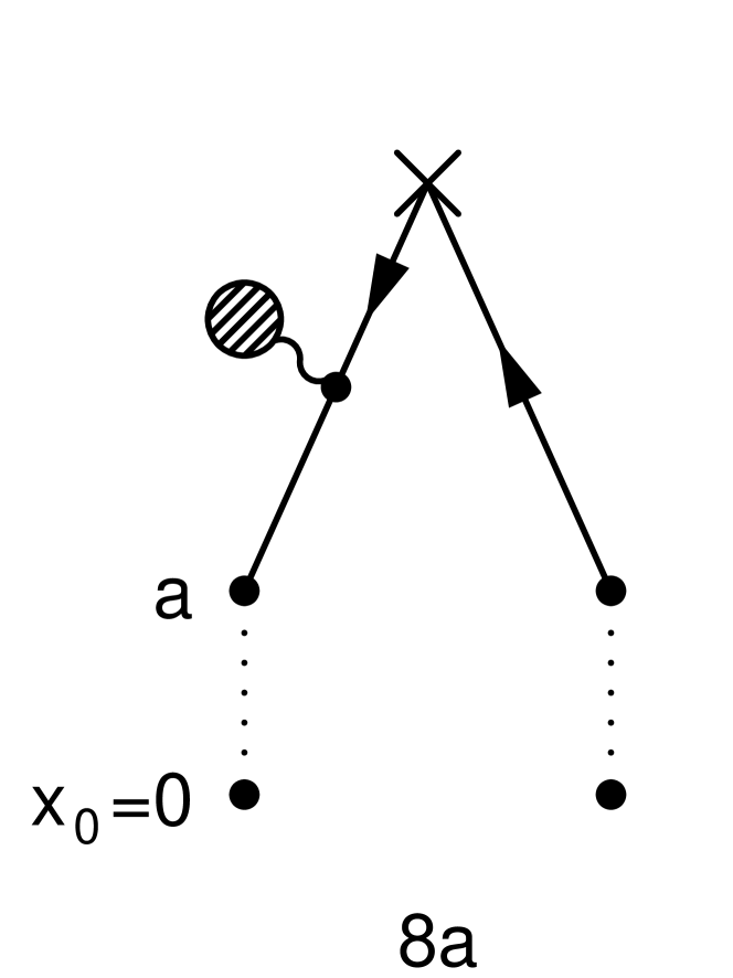
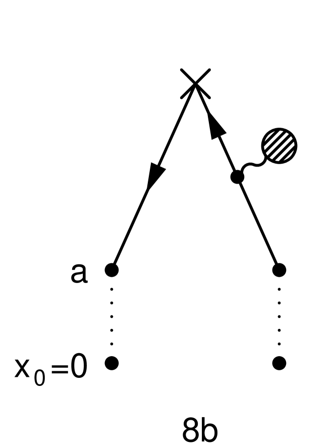
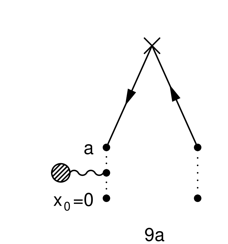
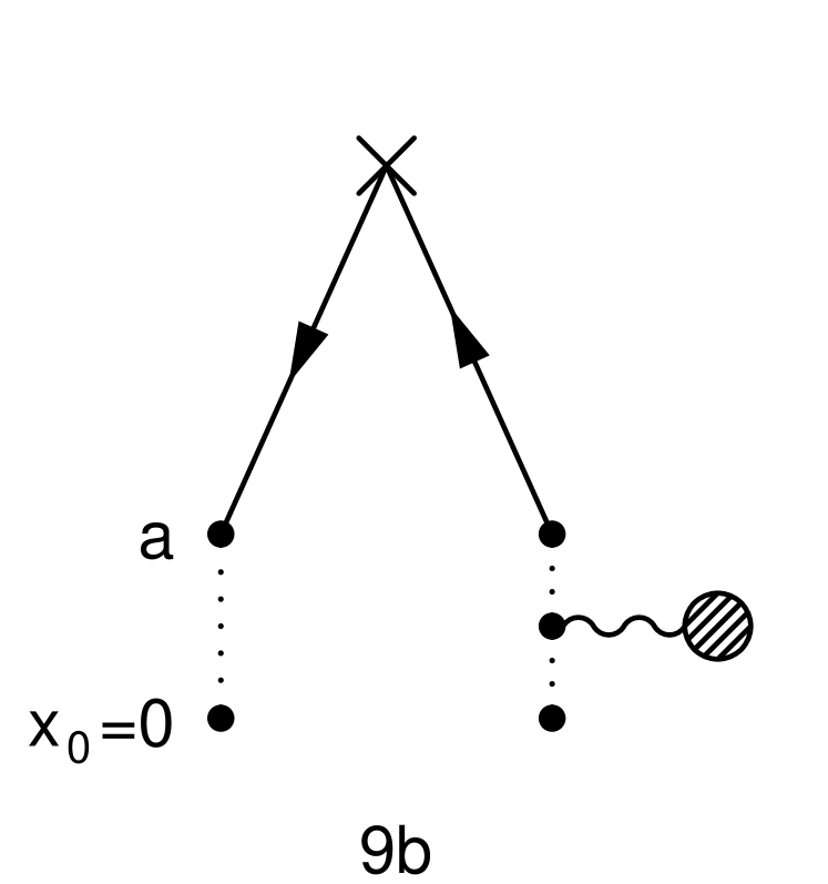
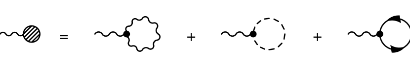
Figure 2: Tadpole diagrams contributing to $f_{A}(x_{0})$ and $f_{P}(x_{0})$ at one loop order of perturbation theory with non–vanishing background field. The dashed line represents the ghost propagator.

The 1–loop correlation functions $f_{A}^{(1)}$ and $f_{P}^{(1)}$ are found by summing all the diagrams. We are now able to compute $m_{c}^{(1)}$ and thus get the deviation $\delta(u,a/L)$ up to 2–loop order. The results are shown in tables 1 and 2. As stated before, the 2–loop coefficients $\delta_{2j}$ are found to be small.

4 Monte Carlo simulations with Bermions

4.1 The bermion model

In the following, we will especially be interested in the theory in which the number of flavours has been continued to $N_{\rm f}=-2$ [11, 10, 12]. This has to be done after the integration over the fermion fields has been performed. At $N_{\rm f}=-2$ the partition function

$$Z=\int D[U]e^{-S_{g}}\det(D^{\dagger}D)^{N_{\rm f}/2}$$ (33)

can be written as

$$Z=\int D[U]D[\phi^{+}]D[\phi]e^{-S_{g}-S_{b}}$$ (34)

with a local bosonic action

$$S_{b}[U,\phi]=a^{4}\sum_{x}|(D\phi)(x)|^{2}.$$ (35)

Note that, in the actual numerical simulation, we have used the hopping parameter representation $M$ of the Dirac operator, which is related to $D$ by

$$M=2\kappa(D+m_{0}),\qquad\kappa=(8+2am_{0})^{-1}.$$ (36)

In a similar way, we can express expectation values of fermionic observables at $N_{\rm f}=-2$ after integration over the quark fields by expectation values in the bermion theory. As an a priori guess consistent with 2-loop perturbation theory, we chose the improvement coefficient $c_{\rm sw}$ by linearly extrapolating the non perturbative results at $N_{\rm f}=2$ and $N_{\rm f}=0$,

$$c_{\rm sw}(g_{0})\bigr{|}_{N_{\rm f}=-2}=2c_{\rm sw}(g_{0})\big{|}_{N_{\rm f}=0}-c_{\rm sw}(g_{0})\big{|}_{N_{\rm f}=2}.$$ (37)

This choice guarantees that the observables are smooth functions of the bare coupling and an extrapolation to the continuum limit is feasible. Furthermore, we have also computed the value for $c_{\rm sw}$ for the most critical parameters used in this work along the lines of [22] and found good agreement with (37), see the next subsection. For the other improvement coefficients, we take the perturbative results with their explicit respective $N_{\rm f}$ dependence.

In the bermion model, the occurrence of Dirac operator zero modes is dynamically enhanced. Thus, in situations in which zero modes (or exceptional configurations) are to be expected, such as large physical volumes or large values for the bare coupling, these may render the functional integral ill-defined or at least hamper its Monte Carlo evaluation. However, we will study this theory not too far from the perturbative regime so that these problems do not occur. Already in the quenched approximation, exceptional configurations occur and invalidate measured fermionic correlation functions. To reach larger couplings, one could also here consider a twisted mass term [23, 24], which we shall however not pursue in this paper.

4.2 The size of $c_{\rm sw}$

In perturbation theory, $c_{\rm sw}$ is linear in $N_{\rm f}$ up to two loops, which motivated us to first do a linear extrapolation of existing non-perturbative data. To corroborate this further, we have computed $c_{\rm sw}$ also non-perturbatively at $N_{\rm f}=-2$ for the bare coupling $\beta=8.99$, which was used in our simulations, compare table 5. The computation was done along the lines of ref [22], to which we refer for unexplained notation and an explanation of the method.

We have computed the current mass $aM$ and the lattice artefact $a\Delta M$ for various values of $\kappa$ at three trial values of $c_{\rm sw}$. As seen before in [5] and [19], we note that $\Delta M$ depends only weakly on the mass $M$. Therefore, we are satisfied with a current mass $M$ that roughly vanishes, thereby introducing a negligible error. Our results for the lattice artefact are summarized in table 3.

$c_{\rm sw}$	$aM$	$a\Delta M$
1.171815	0.0095(1)	0.00218(19)
1.271815	-0.0003(2)	0.00066(24)
1.371815	0.0006(2)	-0.00127(21)

Table 3: $a\Delta M$ at three trial values of $c_{\rm sw}$ at $\beta=8.99$.

A linear interpolation of these three points to the improvement condition $a\Delta M=0.000277$ yields $c_{\rm sw}=1.285(7)$, which is to be compared with the value $c_{\rm sw}=1.271815$ used in the simulation. The effect of this difference in $c_{\rm sw}$ on the step scaling function can be estimated at 1-loop order of perturbation theory. For all lattice sizes, the change in $\Sigma(u,a/L)$ is smaller than $4\times 10^{-4}$, which is negligible compared to the statistical errors, compare table 6.

4.3 Simulation algorithm

Unimproved Wilson bermions can be simulated with a hybrid overrelaxation algorithm, in which the gauge fields are generated by a combination of heatbath and overrelaxation steps and the bermion fields are generated by overrelaxation steps only [12]. Since the improved bosonic action depends quadratically on an individual gauge link $U(x,\mu)$ through the clover term, we found it practically impossible to generalize finite step size algorithms to simulations of improved bermions. A local (link by link) hybrid Monte Carlo algorithm would be feasible and experience from pure gauge theory shows that it is worthwhile to consider it [25]. However, for the same reason as above, a part of the force would have to be recomputed at each step on the trajectory. Thus we expect that such an algorithm would be very expensive. Also a global hybrid Monte Carlo algorithm would be expensive, of course.

Therefore, we decided to perform global heatbath steps for the bosonic field and local overrelaxation steps with respect to the unimproved action for the gauge fields. The clover term is then taken into account in an acceptance step in which the local action difference with respect to the full improved action is used. The acceptance rate in this step turns out to be large enough to pursue this algorithm. As the overrelaxation step can be set up symmetrically, the combined update fulfils detailed balance. Together with the heatbath step for the bosonic field, our algorithm also satisfies ergodicity.

In principle, boson fields $\phi^{\prime}$ with the correct distribution can be generated by drawing a random field $\eta$ from a Gaussian distribution and then applying $\phi^{\prime}=M^{-1}\eta$. However, this procedure is expensive because it requires to run a solver with full accuracy for each update. A method published in [26], which is based on an approximate inversion followed by an additional acceptance step, allows to reduce the cost of this step.

For the update of the gauge fields, we perform a sweep over the lattice and update the links sequentially. By an overrelaxation step with respect to the unimproved action we propose a new configuration $U^{\prime}$ which differs from the old configuration only for the link variable $U(x,\mu)\rightarrow U^{\prime}(x,\mu)$. Thus, for the acceptance step, only the part of the action that depends on this link variable is needed. For the gauge part of the action, the difference

$$S_{g}[U^{\prime}]-S_{g}[U]=-\frac{\beta}{3}\mbox{Re}\mbox{Tr}\Big{(}\big{(}U^{\prime}(x,\mu)-U(x,\mu)\big{)}S^{\dagger}(x,\mu)\Big{)}$$ (38)

can easily be obtained. Here, $S^{\dagger}(x,\mu)$ is the sum of the staples at $(x,\mu)$ and $\beta=6/g_{0}^{2}$.

The bermion contribution can also be computed as a local difference. At the beginning of a sweep through the lattice, the Dirac operator is applied on the whole lattice, and the auxiliary field $\psi=M[U]\phi$ is stored. In each local step, $\psi^{\prime}=M[U^{\prime}]\phi$ is computed from $\psi$ by modifying it at those lattice sites that depend on the link variable $U(x,\mu)$ either through the hopping or through the clover term. In order to simplify our notation, we split $M=M_{1}+M_{2}$ into a term $M_{1}$ which is diagonal in coordinate space and a term $M_{2}$ which contains nearest-neighbour contributions. Then we need to compute

$$\Delta^{(1)}_{x\mu}\phi(z) = M_{1}[U^{\prime}]\phi(z)-M_{1}[U]\phi(z),$$

$$\Delta^{(2)}_{x\mu}\phi(z) = M_{2}[U^{\prime}]\phi(z)-M_{2}[U]\phi(z).$$ (39)

Two lattice sites are affected by the hopping term,

$$\Delta^{(2)}_{x\mu}\phi(x) = -\kappa\lambda_{\mu}\ (1-\gamma_{\mu})\ \big{(}U^{\prime}(x,\mu)-U(x,\mu)\big{)}\ \phi(x+a\hat{\mu}),$$

$$\Delta^{(2)}_{x\mu}\phi(x+a\hat{\mu}) = -\kappa\lambda_{\mu}^{*}\ (1+\gamma_{\mu})\ \big{(}U^{\prime\dagger}(x,\mu)-U^{\dagger}(x,\mu)\big{)}\ \phi(x).$$ (40)

Here $\lambda_{0}=1,\lambda_{k}=e^{i\theta}$. Fourteen lattice sites are affected by the clover term, namely $x$, $x+\hat{\mu}$ and for all directions $\nu\neq\mu\$ $x\pm\hat{\nu}$ and $x+\hat{\mu}\pm\hat{\nu}$. At $x$ we get for example

$$\Delta^{(1)}_{x\mu}\phi(x) = \frac{i}{8}\kappa c_{\rm sw}\big{(}U^{\prime}(x,\mu)-U(x,\mu)\big{)}\times$$ (41)

$$\times\sum_{\nu\neq\mu}\sigma_{\mu\nu}U(x+a\hat{\mu},\nu)U^{\dagger}(x+a\hat{\nu},\mu)U^{\dagger}(x,\nu),$$

and similar terms at the other points. Since the update is local, one has to be careful in parallelizing the algorithm. In a simulation of a lattice on our SIMD machine with only two lattice points per node in any direction, neighbouring nodes would modify the $\psi$ field at a given point simultaneously through the clover term. To avoid this conflict, the local lattice size per node in each direction has to be larger or equal to three.

4.4 Performance

As a measure for the efficiency of our algorithm, we use the machine dependent quantity $M_{\rm cost}$ focusing on the Schrödinger functional coupling $\bar{g}^{2}$. It is defined as

$$M_{\rm cost} =$$ (update time in seconds on machine M) (42)

$$\times(\mbox{error of $1/\bar{g}^{2}$})^{2}\times(4a/T)\,(4a/L)^{3}.$$

In our case, $M_{\rm cost}$ refers to the CPU time spent on an 8-node machine with APE100 architecture. This performance measure allows us to compare for example with performance data obtained in [27] for full QCD.

A further important indicator of the efficiency of the algorithm explained above is the acceptance rate of the clover term in the gauge field update. This acceptance rate turns out to depend only weakly on the parameters in the range of couplings considered here. At $\bar{g}^{2}=0.9793$, it is about $76\%$, while at $\bar{g}^{2}=1.5145$, the acceptance is roughly $70\%$.

The cost of our simulations can in principle be optimized by tuning the precision of the solver in the boson field update. We could however only obtain a total advantage compared to a full precision solver of roughly $10\%$ on the small lattices, with a rather flat minimum. This can mainly be attributed to the fact that the time of an update step is dominated by the gauge field update. Since the optimal size of the residue has to be scaled down when increasing the lattice size [26], this advantage gets even smaller on larger lattices. Hence, we expect for our application that tuning the precision parameter on large lattices is more expensive than running with an ad hoc guess.

The cost at $\bar{g}^{2}=0.9793$ for various lattice sizes for the improved and the unimproved bermion theory is shown in table 4.

$L/a$	$M_{\rm cost}$	$M_{\rm cost}$
	improved	unimproved
4	0.061(2)	0.00535(7)
5	0.107(3)	0.00866(13)
6	0.212(6)	0.0155(2)
8	0.457(11)	0.0319(4)
10	0.790(17)
12	1.30(3)	0.0788(12)

Table 4: Costs for improved bermions in comparison with Wilson bermions at $u=0.9793$. Note that the last two entries for improved bermions are at $u\approx 1.11$.

Obviously, improvement of bermions (with the algorithms explained above) leads to a substantial increase in computer time, which we estimate to be a factor 12. In section 5, it will become clear however, that it is still profitable. The data of table 4 are also shown in figure 3.

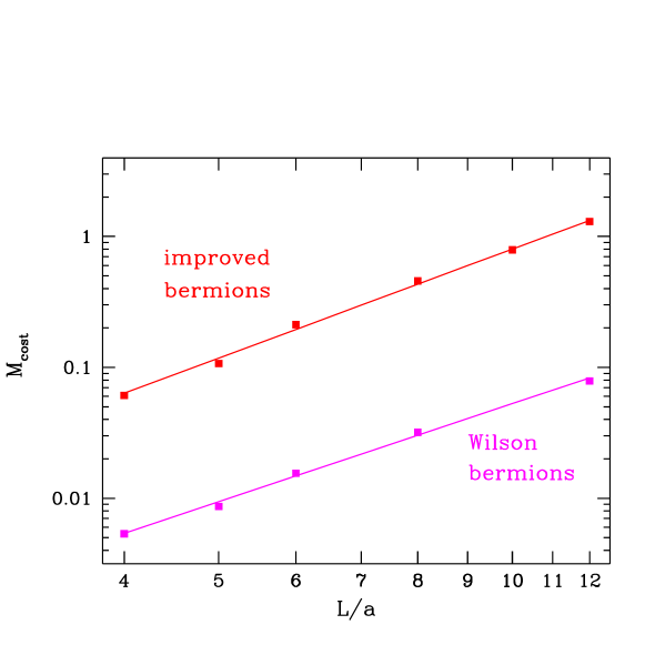
Figure 3: Costs for the measurement of the coupling $u=0.9793$ for Wilson bermions and improved bermions.

A linear fit in this plot (that excludes the smallest lattices of the improved theory) shows that in the improved as well as in the unimproved theory, $M_{\rm cost}$ scales as $a^{-2.5}$.

Comparing with data from [27], it turns out that improved bermions in our implementation are roughly a factor 10 cheaper than simulations in full QCD with two flavours. Furthermore, the scaling with $a$ seems to be slightly better for the bermions. On the other hand, we have estimated the additional cost of unimproved bermions in comparison to pure gauge theory to be only a factor 3.

5 Technical details and results

5.1 Parameters

We have computed the step scaling function $\Sigma(u,\frac{a}{L})$ for the two values of the coupling $u=0.9793$ and $u=1.5145$ at lattice sizes $L/a=4,5,6,8$. To this end, the bare parameters $\beta$ and $\kappa$ have to be tuned such that these couplings are reached while the current masses $m_{1}(L/a)$ vanish. The precision required in the tuning of $\kappa$ can be estimated in perturbation theory [28]. In order to estimate the effect of a slight mismatch in the tuning of $m_{1}$, one defines the derivative of $\Sigma$ with respect to $z=L\ m_{1}$,

$$\frac{\partial}{\partial z}\left.\left(\bar{g}^{2}(2L)\big{|}_{\bar{g}^{2}(L)=u,\ m_{1}(L)=z/L}\right)\right|_{z=0}=\Sigma^{\prime}_{1}(a/L)\ u^{2}+\ldots.$$ (43)

Under the assumption that it suffices to approximate $\Sigma^{\prime}_{1}$ by its universal part (valid for $L/a\rightarrow\infty$), we obtain

$$\Sigma^{\prime}_{1}(0)=\left.-\frac{N_{\rm f}}{4\pi}\frac{\partial}{\partial z}c_{1,1}(z)\right|_{z=0}=0.00957\ N_{\rm f}.$$ (44)

Here, $c_{1,1}(z)$ as defined and computed in [16] has been used. This means for example that a tuning of the current mass to zero up to $0.001$ on an $L/a=8$ lattice leads to an error in the step scaling function smaller than $0.0002\ u^{2}$ and even less on the smaller lattices. Table 5 summarizes the results of the tuning procedure. These results allow to neglect the tuning error for the current mass while the error of $\bar{g}^{2}(L)$ is propagated into the step scaling function by perturbation theory. In those cases where $m_{1}=0$ is displayed in the table, this is a result of an interpolation in the best tuning runs, which is justified by very small values of $\chi^{2}$ obtained in the interpolation.

$\beta$	$\kappa$	$L/a$	$\bar{g}^{2}(L)$	$m_{1}(L/a)$
10.3488	0.131024	4	0.9793(19)	0.00000(31)
10.5617	0.130797	5	0.9795(21)	0.00055(13)
10.7302	0.130686	6	0.9793(11)	0.00000(5)
11.0026	0.130489	8	0.9793(14)	0.00000(6)
8.3378	0.132959	4	1.5145(23)	0.00000(28)
8.5453	0.132637	5	1.5145(17)	0.00000(7)
8.70830	0.132433	6	1.5145(33)	0.00000(4)
8.99	0.13209	8	1.5145(33)	0.00066(8)

Table 5: Parameters and results for the coupling and the mass at $L$.

5.2 The numerical simulation

Most of our numerical simulations were performed on APE100/Quadrics parallel computers with SIMD architecture and single precision arithmetic. We have used machines with up to 256 nodes with an approximate peak performance of 50 MFlops per node. Roughly half of the statistics for the simulation at $L/a=16$ and $u=1.5145$ has been accumulated on one crate (128 nodes) of an APEmille installation in Zeuthen. Since our program was not yet really optimized for APEmille, the advantage is only a factor 3. In our simulations, we have made much use of trivial (replica) parallelization.

The coupling and other inexpensive observables have been measured after each update, which corresponds to a bosonic heatbath step followed by an overrelaxation step for the gauge fields. The fermionic correlation functions to obtain the current mass $m_{1}$ have been measured only rarely, e.g. every 100th update sweep, because the mass does not fluctuate much. We have done up to $16\times 31500$ full updates and measurements of the coupling. The statistical errors of the observables have been determined by a direct computation of the autocorrelation matrix along the lines of appendix A of [27]. Typical autocorrelation times for the coupling range from 3 to 10 (in units of updates).

5.3 Discussion of results

For the non-perturbative computation of the step scaling function, we have simulated pairs of lattices with size $L$ and $2L$ at the same bare parameters in the bermion theory. The results of these computations are listed in table 6.

$L/a$	$\bar{g}^{2}(L)$	$\bar{g}^{2}(2L)$	$m_{1}(2L/a)$
4	0.9793(19)	1.1090(28)	-0.00300(10)
5	0.9795(21)	1.1079(29)	-0.00086(5)
6	0.9793(11)	1.1053(30)	-0.00094(4)
8	0.9793(14)	1.1093(40)	-0.00025(3)
4	1.5145(23)	1.8734(74)	-0.00266(12)
5	1.5145(17)	1.8648(82)	-0.00094(7)
6	1.5145(33)	1.8488(86)	-0.00070(5)
8	1.5145(33)	1.869(14)	0.00002(5)

Table 6: Results for the coupling and the mass at $2L$ at the parameters defined by the given value of $\bar{g}^{2}(L)$.

For the propagation of the statistical error and the mismatch of the tuning results for the coupling, we use a perturbative ansatz. Then we obtain the lattice step scaling function $\Sigma(u,a/L)$ that is shown in figure 4.

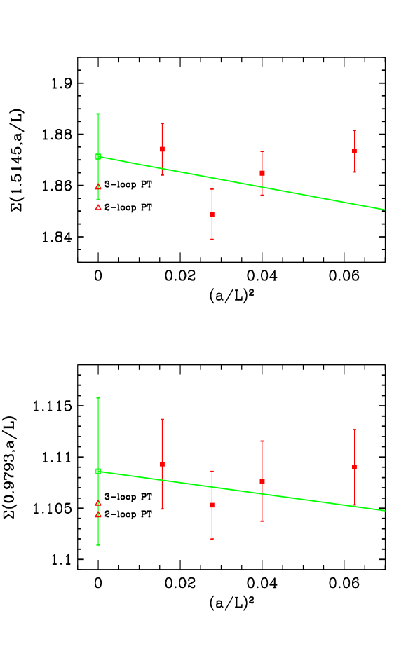
Figure 4: Step scaling function for improved bermions for the couplings $u=0.9793$ and $u=1.5145$ with fits linear in $(a/L)^{2}$. Shown is also the extrapolated continuum value and the 2- and 3-loop results.

We pass to the continuum limit by an extrapolation in $a/L$ with the ansatz

$$\Sigma(u,a/L)=\sigma(u)\ (1+\rho(u)(a/L)^{2}).$$ (45)

As shown in figure 4, this ansatz works perfectly, i.e. within the error bars no linear dependence of the step scaling function on $a/L$ can be detected. The results for the continuum step scaling function and the corresponding 2- and 3-loop values are given in table 7.

$u$	$\sigma(u)$	$\sigma(u)|_{\mbox{\footnotesize 2-loop}}$	$\sigma(u)|_{\mbox{\footnotesize 3-loop}}$
0.9793	1.1063(46)	1.10435	1.10691
1.5145	1.871(17)	1.85122	1.87026

Table 7: Extrapolated simulation results and perturbation theory for the step scaling function at $N_{\rm f}=-2$.

The difference between 2- and 3-loop perturbation theory is thus of the same size as the error of the extrapolated simulation results. Within the error bars, both values of the step scaling function $\sigma(u)$ are consistent with perturbation theory.

The typical size of the ${\rm O}(a)$ effects can be estimated by considering the step scaling function in the unimproved bermion theory as well. This has been done in [12] for $u=0.9793$. Figure 5

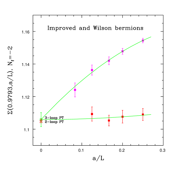
Figure 5: Results for the step scaling function at $u=0.9793$, together with a quadratic fit under the constraint of universality.

shows these results together with the data after implementing improvement. Obviously, the linear cutoff effects are quite seizable for this observable, of the order of a few percent. The data are fitted with a combined fit under the constraint that their continuum limit agrees, that means assuming universality. This fit is linear plus quadratic in $a/L$ for the Wilson bermion data and quadratic in $a/L$ in the improved data. Although the additional input from the Wilson data is included, the joint continuum limit $\sigma_{\rm combined}(0.9793)=1.1059(43)$ agrees almost completely with the value in table 7. A linear plus quadratic fit in $a/L$ of the unimproved data alone would have given the continuum result $\sigma_{\rm unimproved}(0.9793)=1.103(12)$.

The uncertainties of these extrapolated values show a remarkable success of improvement. Although the total computer time for the improved simulations was only by a factor $1.7$ higher than for the Wilson bermions, the error after extrapolation is by a factor $2.7$ smaller. Since a large portion of the computational cost for $\sigma(u)$ comes from the largest lattice, this advantage can be attributed to the lattice size needed for a reasonable extrapolation. For Wilson bermions, this was $L/a=24$, whereas simulations are limited to $L/a=16$ for the improved case. Of course, our observation is restricted to one value of the coupling; at different values, lattice artefacts may behave differently. It should also be noted that in the bermion case, adding the clover term leads to a significant performance penalty for the numerical simulation. For typical algorithms for the simulation of dynamical fermions, like variants of the Hybrid Monte Carlo, the inclusion of the clover term implies a much smaller overhead. Hence, the advantage of improvement should be even bigger there.

In addition to our determination of the step scaling function by extrapolating $\Sigma(u,L/a)$ from Monte Carlo simulations, we have also analysed the approach to the continuum limit for data which have the 2-loop perturbative lattice artefacts cancelled. To this end, we replace the lattice step scaling used for the fit by the corrected values

$$\Sigma^{(2)}(u,a/L)=\frac{\Sigma(u,a/L)}{1+\delta_{1}(a/L)u+\delta_{2}(a/L)u^{2}}$$ (46)

with $\delta$ from  (15). The results for these fits are shown in figure 6, together with the uncorrected fits shown before in figure 4. Again, we leave out the point at $L/a=4$ for the fits. As can be seen from the plot, this procedure does not visibly reduce remaining lattice artefacts. For the coupling $u=1.5145$, the slope of the fitted line gets slightly smaller, whereas for $u=0.9793$ it remains roughly equal. However, if we also include the point at $L/a=4$, the lattice artefacts have even larger ${\rm O}(a)^{2}$ effects than for the uncorrected data. Nevertheless, their continuum limit agrees within the error bars with the one obtained by the procedure used before. It is also consistent with perturbation theory in the continuum limit.

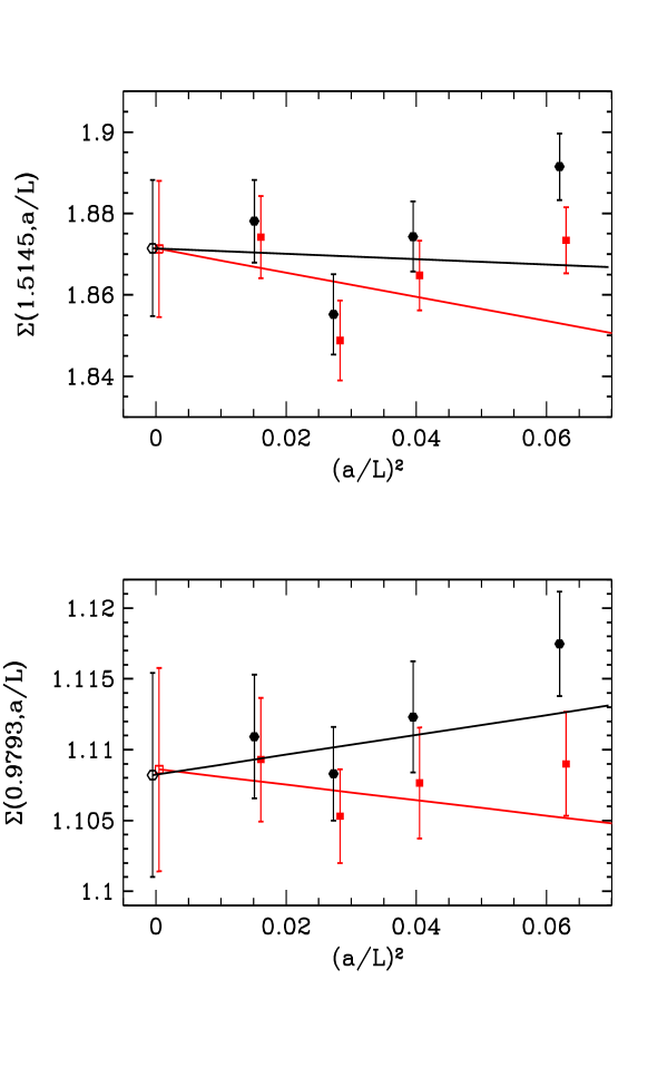
Figure 6: Step scaling function for improved bermions for the couplings $u=0.9793$ and $u=1.5145$ with fits linear in $(a/L)^{2}$. The rectangles represent the data points obtained from our simulations, whereas the circles represent the data $\Sigma^{(2)}$ corrected by perturbation theory.

Since the mass $m_{1}$ is tuned to zero on the small lattices, we expect that $L\big{(}m_{1}(2L)-m_{1}(L)\big{)}$ is a pure lattice artefact that vanishes in the continuum limit with a rate proportional to $(a/L)^{2}$. This expectation is confirmed by figure 7 in which

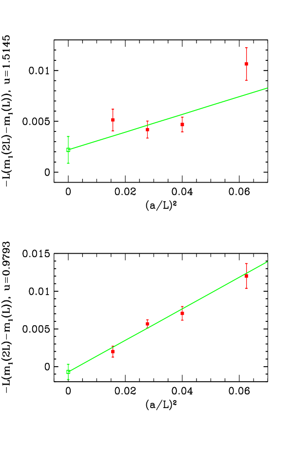
Figure 7: Check of lattice artefacts in the mass at $u=0.9793$ and $u=1.5145$.

this mass difference is shown as a function of $(a/L)^{2}$. While the scaling is perfect for the smaller of the two couplings, there are small deviations at $u=1.5145$, which however can be attributed to statistical fluctuations.

6 Conclusions

In this paper, we have investigated the step scaling function in the ${\rm O}(a)$ improved bermion model by means of extrapolating Monte Carlo data at different lattice resolutions to the continuum limit. The results obtained were compared with renormalized perturbation theory in the continuum limit and with data obtained from simulation of unimproved bermions. They also serve as a guide in planning analogous simulations with dynamical quarks.

It is demonstrated that the implementation of improvement successfully reduces lattice artefacts and allows a fit of the step scaling function $\Sigma(u,a/L)$ linearly in $(a/L)^{2}$ (see figure 5). This raises our confidence that the same extrapolation procedure can be applied for dynamical fermions. We note however, that to our disappointment, the computer time required for our algorithm turned out to be only about a factor $10$ smaller than for dynamical fermions. This means that the lattice sizes that can be reached are not much larger than for fermions, in contrast to the situation without improvement.

Acknowledgements. We would like to thank Peter Weisz for essential checks on our perturbative calculations and Rainer Sommer for helpful discussions. DESY provided us with the necessary computing resources and the APE group contributed their permanent assistance. This work is supported by the Deutsche Forschungsgemeinschaft under Graduiertenkolleg GK 271 and by the European Community’s Human Potential Programme under contract HPRN-CT-2000-00145.

References

- [1] P. Weisz, Nucl. Phys. Proc. Suppl., 47:71–83, 1996. hep-lat/9511017.
- [2] Martin Lüscher, Peter Weisz, and Ulli Wolff, Nucl. Phys., B359:221–243, 1991.
- [3] Martin Lüscher, Rajamani Narayanan, Peter Weisz, and Ulli Wolff, Nucl.Phys. B384, pages 168–228, 1992. hep-lat/9207009.
- [4] Stefan Sint, Nucl. Phys., B421:135–158, 1994. hep-lat/9312079.
- [5] Martin Lüscher, Stefan Sint, Rainer Sommer, Peter Weisz, and Ulli Wolff, Nucl. Phys., B491:323–343, 1997. hep-lat/9609035.
- [6] Giulia de Divitiis et al., Nucl. Phys., B437:447–470, 1995. hep-lat/9411017.
- [7] Martin Lüscher, Rainer Sommer, Peter Weisz, and Ulli Wolff, Nucl. Phys. B413, pages 481–502, 1994. hep-lat/9309005.
- [8] Joyce Garden, Jochen Heitger, Rainer Sommer, and Hartmut Wittig, Nucl. Phys., B571:237–256, 2000. hep-lat/9906013.
- [9] Achim Bode et al. [ALPHA collaboration], 2001. hep-lat/0105003.
- [10] G. M. de Divitiis, R. Frezzotti, M. Guagnelli, M. Masetti, and R. Petronzio, Nucl.Phys., B455:274, 1995. hep-lat/9507020.
- [11] S. J. Anthony, C. H. Llewellyn Smith, and J. F. Wheater, Phys. Lett., B116:287, 1982.
- [12] Juri Rolf and Ulli Wolff, Nucl. Phys. Proc. Suppl., 83:899–901, 2000. hep-lat/9907007.
- [13] Achim Bode, Peter Weisz, and Ulli Wolff, Nucl. Phys., B576:517–539, 2000. Erratum-ibid. B600:453,2001. hep-lat/9911018v3.
- [14] Martin Lüscher, Stefan Sint, Rainer Sommer, and Peter Weisz, Nucl. Phys., B478:365–400, 1996. hep-lat/9605038.
- [15] M. Lüscher and P. Weisz, Nucl. Phys., B479:429–458, 1996. hep-lat/9606016.
- [16] Stefan Sint and Rainer Sommer, Nucl. Phys., B465:71–98, 1996. hep-lat/9508012.
- [17] B. Sheikholeslami and R. Wohlert, Nucl. Phys., B259:572, 1985.
- [18] R. Wohlert. DESY 87/069.
- [19] Karl Jansen and Rainer Sommer, Nucl. Phys. Proc. Suppl., 63:853–855, 1998. hep-lat/9709022.
- [20] Karl Jansen et al., Phys. Lett., B372:275–282, 1996. hep-lat/9512009.
- [21] Rajamani Narayanan and Ulli Wolff, Nucl. Phys., B444:425, 1995. hep-lat/9502021.
- [22] Karl Jansen and Rainer Sommer, Nucl. Phys., B530:185–203, 1998. hep-lat/9803017.
- [23] Roberto Frezzotti, Pietro Antonio Grassi, Stefan Sint, and Peter Weisz, Nucl. Phys. Proc. Suppl., 83:941–946, 2000. hep-lat/9909003.
- [24] Roberto Frezzotti, Pietro Antonio Grassi, Stefan Sint, and Peter Weisz, 2001. hep-lat/0101001.
- [25] Bernd Gehrmann and Ulli Wolff, Nucl. Phys. Proc. Suppl., 83:801–803, 2000. hep-lat/9908003.
- [26] Philippe de Forcrand, Phys. Rev., E59:3698–3701, 1999. cond-mat/9811025.
- [27] Roberto Frezzotti, Martin Hasenbusch, Ulli Wolff, Jochen Heitger, and Karl Jansen, Comput. Phys. Commun., 136:1–13, 2001. hep-lat/0009027.
- [28] Rainer Sommer. The step scaling function with two flavours of massless Wilson quarks, 1998. unpublished.