Combining LSND and Atmospheric Anomalies

in a Three-Neutrino Picture

Gabriela Barenboim ^a,b, Amol Dighe ^a,c and Solveig Skadhauge ^d

^a CERN - TH Division, CH-1211 Geneva 23, Switzerland.

^b FERMILAB Theory Group, MS 106, P.O.Box 500, Batavia IL 60510, USA.

^c Max-Planck-Institut für Physik, Föhringer Ring 6, D-80805 Munich, Germany.

^d Department of Mathematical Physics, LTH, Lund University, S-22100 Lund, Sweden.

May 2001

ABSTRACT

We investigate the three-neutrino mixing scheme for solving the atmospheric and LSND anomalies. We find the region in the parameter space that provides a good fit to the LSND and the SK atmospheric data, taking into account the CHOOZ constraint. We demonstrate that the goodness of this fit is comparable to that of the conventional fit to the solar and atmospheric data. Large values of the LSND angle are favoured and $\sin^{2}(2\theta_{\rm LSND})$ can be as high as 0.1. This can have important effects on the atmospheric electron neutrino ratios as well as on down-going multi-GeV muon neutrino ratios. We examine the possibility of distinguishing this scheme from the conventional one at the long baseline experiments. We find that the number of electron neutrino events observed at the CERN to Gran Sasso experiment may lead us to identify the scheme, and hence the mass pattern of neutrinos.

1 Introduction

The present data from the experiments on atmospheric, solar and accelerator (LSND) neutrinos indicate neutrino flavour oscillations. The data from each of these sets of experiments individually can be explained by a single dominant mass square difference $\Delta m^{2}$ and a mixing angle $\theta$ between two active neutrinos. The atmospheric neutrino data from SuperKamiokande (SK) [1] indicate $\nu_{\mu}\leftrightarrow\nu_{\tau}$ as the dominant mode, with $\Delta m^{2}_{\rm atm}=(1$ - $8)\times 10^{-3}\mbox{ eV}^{2},\sin^{2}2\theta=0.8$ - $1.0$. The three MSW solutions (LMA, SMA and LOW) as well as the vacuum oscillations can provide reasonable fits to the solar neutrino data [2, 3, 4, 5] and all these solutions have $\Delta m^{2}_{\odot}\leq 2\times 10^{-4}$ eV². The results of the LSND experiment [6, 7] are neither confirmed nor fully excluded by the KARMEN2 data [8], and the combined fit allows a region [9] of $\Delta m^{2}_{LSND}=(0.1$ - $1)\mbox{ eV}^{2},\sin^{2}2\theta_{\mu e}\approx 10^{-3}-10^{-2}$. There are also constraints on the mixing of $\nu_{e}$ from the CHOOZ experiment [10]: we have $\sin^{2}2\theta_{e}\leq 0.1$ for $\Delta m^{2}>10^{-3}$ eV².

In the context of only three known neutrino species, the $\Delta m^{2}$s corresponding to the solutions of the three neutrino anomalies above (atmospheric, solar and LSND) cannot be reconciled. The three-neutrino schemes make a very poor fit to all the data. Two ways are possible out of this predicament: (i) turn a blind eye to one of the experiments and fit for the other two in three-neutrino schemes; (ii) solve two of the neutrino anomalies with three-neutrino oscillations and solve the third one by using exotic models such as sterile neutrinos, FCNC, neutrino decay, extra dimensions, etc.

Since the LSND result is yet to be confirmed, it is customary to ignore it and accommodate the solar neutrino deficit and the atmospheric anomaly with the mixing between three active neutrinos. Implicit in this is the assumption that the LSND results will be proved false by future experiments, which can be justified by the fact that KARMEN2 [8] and Bugey [11] already rule out most of the allowed region of LSND. However, this is just a convenient assumption, and the possibility of the LSND results being confirmed by future experiments such as BooNe [12] cannot be ignored. Also the new analysis of the final data by the LSND collaboration [7] is consistent with the old results [6], and therefore strengthens the anomaly evidence.

Our approach will be to study the neutrino anomalies with three-(active)-neutrino oscillation. This allows us to solve only two of the three anomalies. As the atmospheric data are showing strong evidence for neutrino oscillation, thanks to the large range of L/E probed, we will take this to be one of the anomalies solved by oscillation. There is no compelling evidence that the electron neutrinos participate in the oscillations of atmospheric neutrinos. This implies that the $P_{\nu_{e}\rightarrow\nu_{\mu}}$ must be small, meaning either that the mixing angle is small (LSND case) or that the $\Delta m^{2}$ is too small to affect the atmospheric neutrinos (solar case). The large angle solutions to LSND is in any case ruled out by the results of Bugey. Moreover, just from the point of view of goodness of fit (quantified by a $\chi^{2}$ function), the best fits to (I) atmospheric and solar data, and (II) atmospheric and LSND data are equally good (as we shall show in this paper). Scheme II gives a different mass spectrum from the conventional scheme I, and an eye should be kept on future experiments in order to resolve this discrete ambiguity. That we leave out one anomaly does not mean that we do not believe in it, but rather that it has to be solved in some other way.

In the case of solar neutrinos there are various viable “exotic” solutions. The most popular among them is the sterile neutrino SMA MSW solution. In the favoured “2+2” four-neutrino scheme [13], the sterile neutrino participates mainly in the solar neutrino anomaly and the three active neutrinos solve the atmospheric and LSND anomalies among themselves [15]. This is indeed a possible extension of scheme II, and the fit we perform will be a guide for this option. Many other exotic solutions exist for solving the solar neutrino anomaly [14]. Flavour changing neutral current interactions (FCNC) [16] can explain the data well [17] – this solution uses the matter of the Sun to make a FCNC transition, such as $\nu_{e}$ + quark $\rightarrow$ quark + $\nu_{\mu}$. The different neutrino production points gives the necessary energy dependence of the solar neutrino flux. Furthermore a violation of the equivalence principle has been suggested and cannot be excluded. Solutions have also been suggested in the scenarios with large extra dimensions, where the solar neutrino anomaly is accounted for by the mixing with a Kaluza-Klein tower of sterile neutrinos [18] and the three active neutrinos account for the atmospheric and LSND anomalies [19]. A resonant spin-flip conversion [20] of the left-handed neutrino to unobservable right-handed states, due to the solar magnetic field, gives a good fit to the data [21]. This solution cannot be reconciled with LSND and atmospheric anomalies, as the mass squared difference needed is too small ($\approx 10^{-8}$eV²). In the three-neutrino schemes able to account for the atmospheric and LSND result, one of the possible mass patterns has the electron neutrino mainly in the heavy state, and therefore neutrino decay could also be thought of as a way out for explaining the solar anomaly. Although this solution does not agree well with the data.

Some exotic solutions for the LSND anomaly have also been suggested in the literature [22]: for instance, having new flavour-violating decay modes of muons. This possibility cannot yet be ruled out in a model-independent way. The introduction of a sterile neutrino to solve the LSND anomaly gives rise to the “3+1” neutrino mass pattern [23], which is very close to being excluded [24]. It might be argued that the exotic solutions are more likely to solve the solar anomaly than the LSND one, since the matter and the magnetic field, which provide more degrees of freedom for the exotic solutions in the solar case, are absent in the LSND experiment.

There is a vast literature on three-neutrino oscillation fits to atmospheric data [25]. Also the combined fit to solar and atmospheric data is well-explored and is known to describe the data well [26, 27]. Furthermore the two-neutrino $\nu_{\mu}\rightarrow\nu_{\tau}$ oscillation gives a good explanation of the atmospheric data. This solution would be obtained in the limit of a very small LSND angle, and therefore we already know that the LSND and atmospheric data can be reconciled. The important question to answer is if the three-neutrino scheme can fit the data even better and if there are any possible effects that could be observed in the near future.

The three-active-neutrino solution to LSND and atmospheric problems has also been studied in [28], where however only the up/down asymmetries from the atmospheric data were used for the fits. Here we will consider the full set of 40 data points from the sub-GeV and multi-GeV neutrinos observed by the SK collaboration. Furthermore we take into account the data from CHOOZ [10] and the matter effects inside the Earth. We define a $\chi^{2}$ function and perform fits to schemes I and II above, and find that both fits are equally good. We explore further the fit to scheme II. The mass pattern corresponding to this fit may be tested at the long baseline experiments, e.g. K2K [29], MINOS [30] or CNGS [31]. We perform Monte Carlo simulations to check if this mass pattern can be distinguished from the conventional one at these experiments. If BooNE confirms the LSND results, this scheme II, coupled with the appropriate exotic solution for the solar neutrino anomaly, will provide the solution for the mass spectrum of neutrinos.

The paper is organized as follows. In Sec. 2 we perform fits to the data for schemes I and II. In Sec. 3, we compare the signals at the long baseline experiments with the two mass patterns and look for ways of distinguishing between them. Our findings are summarized in Sec. 4.

2 $\chi^{2}$ fits to the data

The aim of this section is to find the regions in the three-neutrino mixing parameter space that describe (I) the atmospheric and solar data and (II) the atmospheric and LSND data. We shall define a $\chi^{2}$ function in order to quantify the goodness of these fits. It is clearly not fair to compare the $\chi^{2}$s from these two fits, since they correspond to different data sets. We perform the fit to scheme I to demonstrate the soundness of our $\chi^{2}$ function by showing that this procedure, rough though it is, reproduces the conventional fits, which are much more accurate [25, 26]. Since our aim here is just to get a broad estimate of the allowed parameter space, this rough fit should suffice for our purpose. Then we follow the same procedure to perform a fit to scheme II and find the allowed region in the parameter space that describes the data reasonably well.

The neutrino mixing matrix $U_{MNS}$ is parametrized as [32]

$$U_{MNS}=\left(\matrix{c_{12}c_{13}&s_{12}c_{13}&s_{13}\cr-s_{12}c_{23}-c_{12}s_{23}s_{13}&c_{12}c_{23}-s_{12}s_{23}s_{13}&s_{23}c_{13}\cr s_{12}s_{23}-c_{12}c_{23}s_{13}&-c_{12}s_{23}-s_{12}c_{23}s_{13}&c_{23}c_{13}}\right)$$ (1)

where we have neglected any $CP$ violation. The mass spectrum is parametrized by five parameters, $s_{12}$, $s_{23}$, $s_{13}$, $\Delta m_{21}^{2}$ and $\Delta m_{31}^{2}$. (Here and in the following $s_{ij}$, $c_{ij}$ are shorthands for $\sin(\theta_{ij})$, $\cos(\theta_{ij})$ respectively, and we use the convention $\Delta m^{2}_{ij}\equiv m^{2}_{i}-m^{2}_{j}$.) We define $\nu_{1}$ as the lightest state and $\nu_{3}$ as the heaviest state.

For both schemes there are two solutions; the normal hierarchy ($\Delta m^{2}_{21}\ll\Delta m^{2}_{32}\simeq\Delta m^{2}_{31}$) and the inverted hierarchy ($\Delta m^{2}_{31}\simeq\Delta m^{2}_{21}\gg\Delta m^{2}_{32}$). Neutrino oscillations in vacuum cannot distinguish between the two hierarchies, but with matter effects, the data could in principle distinguish between them. In scheme I the characteristic features of the normal hierarchy is the small value of $s_{13}$, and the inverted hierarchy corresponds to values of $s_{12}$ close to 1. It has recently been shown that the differences between the two hierarchies within this scheme are very small [33]. For scheme II normal (inverted) hierarchy corresponds to $s_{13}\simeq 1$ ($s_{13},s_{12}\simeq 0$). The matter effects in this scheme are negligible, since both the $\Delta m^{2}_{\rm atm}$ and $\Delta m^{2}_{\rm LSND}$ are too large for the Earth’s density to play any significant part. Therefore, the differences between the predictions from the two hierarchies are extremely small. For both schemes we shall only consider the normal hierarchy while performing the fit. It should be remembered that for each point in the parameter space with normal hierarchy, there exists a corresponding point with inverted hierarchy that gives almost the same value of $\chi^{2}$.

For the atmospheric data, we only consider the SK multi-GeV and sub-GeV data [34]. The mean neutrino energy for the partially contained events and the upward going muons at SK is higher. In this range the effects of a solar mass squared difference are therefore negligible. The small contributions arising from an averaging of a LSND mass sqaured difference can be compensated by a shift towards smaller $\Delta m^{2}_{\rm atm}$ (see section 2.2). Therefore it is not expected that the data will affect the comparison of the two schemes. Nevertheless it might results in small changes in the allowed regions. The further inclusion of the data from other atmospheric neutrino experiments [35] is not expected to affect the fit much, since the number of fully contained events at SK is overwhelmingly large as compared to these.

The experimental data are represented by the ratios $R_{\alpha,i}$ between the experimental values for the fluxes and the theoretical Monte Carlo prediction in the case of no oscillation for muon and electron neutrinos in the 10 different zenith angle bins. The ratios $R_{\alpha,i}$ can be written as

$$R_{\alpha,i}^{\rm exp}=N_{\alpha,i}^{\rm exp}/N_{\alpha,i}^{\rm MC}\;\;\;\;,\;\alpha=\mu,e\;\;,\;i=1\dots 10\;.$$ (2)

The number of events for the sub-GeV neutrinos is calculated as;

$$N_{\alpha} = n_{T}\sum_{\nu,\overline{\nu}}\sum_{\beta=e,\mu}\int_{0}^{\infty}dE_{\nu}\int_{-1}^{1}d\cos(\theta_{\nu})\int_{E_{l,{\rm min}}}^{E_{l,{\rm max}}}dE_{l}\int_{-1}^{1}d\cos(\theta_{l\nu})\frac{1}{2\pi}\int_{0}^{2\pi}d\phi$$ (3)

$$\times \frac{d^{2}\Phi_{\beta}}{dE_{\nu}d\cos(\theta_{\nu})}\frac{d^{2}\sigma_{\beta}}{dE_{l}d\cos(\theta_{l\nu})}P_{\alpha\beta}(E_{\nu},\theta_{\nu})\epsilon(E_{l})\;,$$

where $E_{\nu}$ is the neutrino energy, $E_{l}$ is the lepton energy, $\theta_{l\nu}$ is the angle between the neutrino and the scattered lepton, $\theta_{\nu}$ is the zenith angle of neutrino. The number of target nucleons is denoted by $n_{T}$. $\phi$ is the azimuthal angle of the incoming neutrino, and is used to calculate the zenith angle $\theta_{l}$ of the charged lepton:

$$\cos(\theta_{l})=\cos(\theta_{\nu})\cos(\theta_{\nu l})+\sin(\theta_{\nu})\cos(\phi)\sin(\theta_{l})\;.$$ (4)

For the differential sub-GeV cross section for $\nu_{l}N\rightarrow lX$, we use the quasi-elastic approximation [36], with the sub-GeV fluxes $\Phi$ taken from [37]. The efficiency function $\epsilon(E_{l})$ is not published by the SK collaboration. But as we divide by the SK Monte Carlos, this effect is averaged out if the efficiency function is flat within the different samples.

In the calculations of the multi-GeV ratios we find that the number of events can be well described by

$$N_{l}=n_{T}\int_{E_{l,min}}^{E_{l,max}}dE_{\nu}\int_{-1}^{1}d\cos(\theta_{\nu})\frac{d^{2}\Phi}{dE_{\nu}d\cos(\theta_{\nu})}\sigma_{\alpha}(E_{\nu})P_{\alpha\beta}(E_{\nu},\theta_{\nu})\;.$$ (5)

Here we assume that the energy of the charged lepton is the same as that of the incoming neutrino. In order to account for the scattering angle, we further smear the spectrum with a Gaussian function, where we use the width $\sigma\approx 25^{\circ}$ for the electron neutrinos and $\sigma\approx 15^{\circ}$ for the muons neutrinos [38]. The total cross section for neutrinos is given in [39], and for the antineutrinos we use the approximate formula $\sigma_{\overline{\nu}_{e}}=0.34\times 10^{-38}E_{\nu}$ cm²/GeV. The multi-GeV fluxes are taken from [40]. A comparison between the ratios obtained from (5) and the ones obtained by using the differential cross section including the quasi-elastic, one pion and deep inelastic channels yields hardly any difference.

The probabilities are calculated taking into account all the mass-squared differences:

$$P_{\alpha\beta}=\delta_{\alpha\beta}-4\sum_{i>j}U_{\alpha i}U_{\beta j}U_{\alpha j}U_{\beta i}\sin^{2}\left(\frac{\Delta m^{2}_{ij}L}{4E}\right)\;,$$ (6)

where all the quantities are calculated in the presence of matter wherever appropriate. Even in the conventional case, the sub-GeV ratios in particular are influenced also by the small mass squared difference [41]. The oscillation length $L$ depends on the zenith angle of the neutrino:

$$L=\sqrt{(R_{E}+h)^{2}-R_{E}^{2}\sin^{2}(\theta_{\nu})}-R_{E}\cos(\theta_{\nu})\;,$$ (7)

where $R_{E}$ is the radius of the Earth and $h$ is the production height of the neutrinos in the atmosphere. We take $h\simeq 10$ km.

Matter effects are important for the atmospheric neutrinos. We simulate the matter effects by using a two-shell model of the matter densities in Earth. The density in the mantle (core) is taken to be roughly 3.35 (8.44) g/cm³, and the core radius is taken to be 2887 km. From this we calculate the average density as a function of the neutrino zenith angle. This allows us to use the three-neutrino mixing matrix in matter, as calculated in [42].

We define the atmospheric $\chi^{2}$ as

$$\chi^{2}_{\rm atm}=\sum_{M,S}\sum_{\alpha=e,\mu}\sum_{i=1}^{10}\frac{(R_{\alpha,i}^{\rm exp}-R_{\alpha,i}^{\rm th})^{2}}{\sigma_{\alpha i}^{2}}\quad,$$ (8)

where $\sigma_{\alpha,i}$ are the statistical errors and $M,S$ stand for the multi-GeV and sub-GeV data respectively. The total number of data points is 40.

From the CHOOZ experiment [10] we use the 15 data points with the statistical errors. The CHOOZ baseline is roughly 1000 m, and the neutrino energy in the range from 3 to 9 MeV. Therefore the $\sin^{2}(\Delta m^{2}L/4E)$ terms do oscillate within the energy region and hence all the data points need to be taken into account. In each bin we average the probability over energy. When including the LSND experiment we use one datum [6]. The distance travelled by the antineutrinos ($\overline{\nu}_{\mu}$) is set to 30 m and we use the mean energy of 42 MeV. When including data from the Bugey experiment [11] we take three data points; $P_{\overline{\nu}_{e}\overline{\nu}_{e}}$ for the three different baselines of 15 m, 40 m, and 95 m. The probability is averaged over the positron energy range 1 - 6 MeV. We take both the statistical and systematic errors, as the systematic errors are large compared to the statistical ones.

The solution to the solar neutrino problem is preferred to be within the LMA region and we will therefore use parameters only within this region in order to make a fit. The $\chi^{2}$ for the solar LMA solution is taken from Ref.[26]. This fit includes the total rates in the chlorine (Homestake) experiment [3], the gallium (SAGE, GALLEX) experiments [4, 5], Kamiokande [43] and SuperKamiokande [2]. Furthermore the spectra for both day and night are included. In total there are 42 data points fitting with three parameters: $\Delta m^{2}_{\odot},\theta_{\odot}$ and the overall flux normalization for the SK spectrum.

The total $\chi^{2}$ function for scheme I is then

$$\chi^{2}_{I}=\chi^{2}_{\rm atm}+\chi^{2}_{\rm CHOOZ}+\chi^{2}_{\rm LMA}~{},$$ (9)

and for scheme II, we have

$$\chi^{2}_{II}=\chi^{2}_{\rm atm}+\chi^{2}_{\rm CHOOZ}+\chi^{2}_{\rm LSND}~{}~{}.$$ (10)

Before interpreting the results, a word of caution is in order. In our analysis (as in the standard procedures), we deal not with the number of observed events but with the ratio of the number of observed events to the number of events expected from the Monte Carlo. These ratios are convenient because they directly give a measure of the survival/oscillation probability. The Monte Carlo predictions, in the case of atmospheric neutrinos fluxes, contain large uncertainties, especially in the absolute values of fluxes. This is the reason why some data are presented in the form of a ratio of two measured quantities and is compared with theoretical predictions of the same ratio. We have not included theoretical uncertainties and correlations in the atmospheric neutrino fluxes. However, a previous analysis [44] has found that they do not affect the fit significantly.

It has been pointed out recently that there is a significant discrepancy between the commonly used primary cosmic ray fluxes and the measured ones [45]. The variation of the primary cosmic ray flux is directly related to the absolute value of the atmospheric neutrino fluxes and can also affect (to a less significant extent) its energy and zenith angle dependence. This may affect the allowed region of the atmospheric neutrino anomaly. It is important to bear in mind that when applying the calculated atmospheric neutrino fluxes to a neutrino oscillation study, the absolute values of the fluxes as well as the tiny variations with energy between them could become important.

2.1 Fit to solar, atmospheric and CHOOZ data (scheme I)

In this section, we perform a fit to the conventional three-neutrino scheme for solving the solar and atmospheric anomalies. When fitting within this scheme we will take $\Delta m_{31}^{2}\simeq 10^{-3}$ - $10^{-2}$ eV² and $\Delta m_{21}^{2}$ suitable to solve the solar neutrino problem. The $\chi^{2}_{\rm atm}$ and $\chi^{2}_{\rm CHOOZ}$ are to a very large extent independent of $s_{12}$. We will therefore keep the solar angle constant at $s_{12}^{2}=0.3$, which is close to the best-fit point of the LMA solution [26]. The small $\Delta m_{21}^{2}$ is taken in the range $2\times 10^{-5}$ - $2\times 10^{-4}$ eV². In particular the electron neutrino ratios can be affected by the solar mass difference [41], and we therefore calculate $\chi^{2}_{\rm atm}+\chi^{2}_{\rm CHOOZ}$ for a few values of $\Delta m^{2}_{\odot}$. We thus have four degrees of freedom, $s_{23},s_{13},\Delta m^{2}_{21},\Delta m^{2}_{31}$.

We first find the best point while doing a combined fit to SK and CHOOZ, with $\chi^{2}\equiv\chi^{2}_{\rm atm}+\chi^{2}_{\rm CHOOZ}$. There are 55 data points: 40 from SK atmospheric data and 15 from CHOOZ. The minimum is $\chi^{2}_{\rm min}=45.3$ at

$$s_{23}^{2}=0.41\;,\;s_{13}^{2}=0.00\;,\;\Delta m_{21}^{2}=2.0\times 10^{-4}\;,\;\Delta m_{31}^{2}=4.1\times 10^{-3}~{}~{}.$$ (11)

Note that the minimum occurs for the largest value in the allowed region for $\Delta m^{2}_{\odot}$. With $\Delta m_{21}^{2}$ constrained to be $2.0\times 10^{-5}$ ($8.0\times 10^{-5}$), the value of $\chi^{2}_{\rm min}$ is $\chi^{2}_{\rm min}=49.1\;(46.9)$ at $s_{23}^{2}=0.58\;(0.40),\>s_{13}^{2}=0.01\;(0.00),\>\Delta m_{31}^{2}=0.0040\;(0.0045)$. We see that the dependence on the solar mass squared difference is weak. The $\chi^{2}$ rises slightly when $\Delta m^{2}_{\odot}$ becomes smaller. For $\Delta m^{2}_{\odot}<10^{-5}$ this dependence is lost and the $\chi^{2}$ function is almost constant.

Figure 1(a) shows the allowed region in $\Delta m^{2}_{31}=\Delta m^{2}_{\rm atm}$ and $4U_{\mu 3}^{2}U_{\tau 3}^{2}\approx\sin^{2}(2\theta_{\rm atm})$. The confidence intervals are calculated for four parameters (as we keep $s_{12}$ fixed), so that the 90% (99%) confidence interval corresponds to $\chi^{2}-\chi^{2}_{\rm min}<7.8\;(13.3)$ [32]. At 99% CL we find $1.75\times 10^{-3}{\rm eV}^{2}<\Delta m^{2}<7.5\times 10^{-3}$ eV² and $\sin^{2}(2\theta_{\rm atm})>0.83$. These bounds are in good agreement with previous analyses [25, 26].

In figure 1(b) we show the 99% CL and the 90% CL area in $s_{13}^{2}$ and $s_{23}^{2}$. At 99% CL the upper bound on $s_{13}^{2}$ is 0.065, corresponding to a value of $\sin^{2}(2\theta_{\rm CHOOZ})\equiv 4U_{e3}^{2}(1-U_{e3}^{2})$ smaller than 0.25.

The full three-neutrino fit is not symmetric around $s_{23}^{2}=0.5$, as is also seen in Fig. 2(a) and (b). The small asymmetries arise from non-zero values of either $s_{13}$ or $\Delta m^{2}_{\odot}$. This may be interpreted in terms of the electron excess (see the discussion in Sec. 3.1).

We now consider the combined fit including the effect of the solar neutrino data in the LMA region. The common parameter, $\Delta m^{2}_{\odot}$, must be taken to be the same, and we calculate $\chi^{2}_{I}$ for a few values of this parameter. The minimum value occurs at $\Delta m^{2}_{\odot}=8\times 10^{-5}$ with $\chi^{2}_{\rm LMA}=37.3$ [26]. Hence when fitting to all three experiments (SK atmospheric, CHOOZ, solar data), we get $\chi^{2}_{I({\rm min})}\approx 84$ with 6 parameters and 97 data points, so that $\chi^{2}_{I({\rm min})}/{\rm dof}\approx$ 0.93.

Recently a fit was performed to the solar data allowing for a free B and hep flux in the Sun [46]. The obtained LMA $\chi^{2}$ was 29.0 for 39 data points with 4 fit parameters, $\Delta m^{2}_{\odot},\theta_{\odot}$ and the fluxes of ⁸B and $hep$ neutrinos. Combining this with our fit for SK and CHOOZ, we would get $\chi^{2}_{I({\rm min})}\approx$ 78 , so that $\chi^{2}_{I({\rm min})}/{\rm dof}\approx$ 0.90. Allowing for an overall normalization of the atmospheric fluxes, as done by the SK collaboration, could in general also improve the goodness of fit for atmospheric data. Let us also note that in Ref. [26] a combined fit to atmospheric, solar and CHOOZ data gave a best fit of $\chi^{2}/{\rm dof}=0.97$.

The LMA solution currently gives the best fit to the solar data, and the fit to the atmospheric data is not affected much by very small solar mass differences. Therefore we expect that the value of $\chi^{2}$ can only be higher in other regions of parameter space than the one computed above.

2.2 Fit to atmospheric, LSND and CHOOZ data (scheme II)

In this section we give the results of fitting to the SK atmospheric, CHOOZ and LSND data and hence will take $\Delta m^{2}_{21}=\Delta m^{2}_{\rm atm}$ and $\Delta m^{2}_{31}\simeq\Delta m^{2}_{32}=\Delta m^{2}_{\rm LSND}$. The SK and CHOOZ data are largely independent of the large $\Delta m^{2}$, which we can therefore freely use to fit the LSND experiment. For every point in parameter space we simply choose to calculate the value of $\Delta m_{31}^{2}$ that fits the LSND data best. The remaining four parameters ($s_{12},s_{23},s_{13},\Delta m^{2}_{21}$) are varied to obtain confidence levels.

Let us first perform a combined fit to the SK and CHOOZ data with $\chi^{2}\equiv\chi^{2}_{\rm atm}+\chi^{2}_{\rm CHOOZ}$, as we did for scheme I in Sec. 2.1 (again we have 55 data points). The confidence levels are calculated for four fitting parameters. Fig.4(a) shows the allowed region in $\Delta m_{\rm atm}^{2}$ and $4U_{\mu 1}^{2}U_{\mu 2}^{2}\simeq\sin^{2}(2\theta_{\rm atm})$. At 99% confidence level the bounds are $4U_{\mu 1}^{2}U_{\mu 2}^{2}>0.8$ and 1 eV${}^{2}<\Delta m^{2}_{\rm atm}<7$ eV². The allowed region is very similar to the one found in the conventional case. It shows that the two-neutrino atmospheric neutrino fit is only slightly affected by the three-neutrino extension in both schemes. Although we note that the region in $\Delta m^{2}_{\rm atm}$ is lowered in scheme II. This is due to the small constant contributions that arise from the averaging of the $\sin^{2}(\Delta m^{2}_{\rm LSND}L/4E)$ terms.

Let us now include the LSND data in the fit. The best-fit point with $\chi^{2}_{II({\rm min})}=44.9$ for the combined fit is obtained at

$$s_{12}^{2}=0.69\;,\;s_{23}^{2}=0.98\;,\;s_{13}^{2}=0.98\;,\;\Delta m_{21}^{2}=0.0031\;,\;\Delta m_{31}^{2}=0.22\;.$$ (12)

This should be compared with the two-neutrino $\nu_{\mu}\rightarrow\nu_{\tau}$ minimum value of $\chi^{2}$ of 49.5 (at $\Delta m^{2}_{\rm atm}=0.0038$). We remind the reader that the LSND datum is chosen to be fitted best. Hence the effects of the three-neutrino scheme are not large, but still significant. The main reason for the lowering of the $\chi^{2}$ is an excess in both sub-GeV and multi-GeV electron neutrino ratios. The goodness of fit to the data, having $\chi^{2}_{\rm II}/{\rm dof}\approx 0.88$ is thus as good as the one obtained to the solar, atmospheric and CHOOZ data in Sec. 2.1.

The LSND probability is

$$P_{\overline{\nu}_{\mu}\rightarrow\overline{\nu}_{e}}\simeq 4U_{e3}^{2}U_{\mu 3}^{2}\sin^{2}\left(\frac{\Delta m_{\rm LSND}^{2}L}{4E}\right)-4U_{e1}U_{e2}U_{\mu 1}U_{\mu 2}\sin^{2}\left(\frac{\Delta m_{\rm atm}^{2}L}{4E}\right)\;,$$ (13)

where the second term is small because of the small value of $\sin^{2}(\Delta m^{2}_{\rm atm}L/4E)$, so that we may define the LSND angle as $\sin^{2}(2\theta_{\rm LSND})\equiv 4U_{e3}^{2}U_{\mu 3}^{2}$. In terms of physical angles, the best-fit point corresponds to $\sin^{2}(2\theta_{\rm atm})=0.99$ and $\sin^{2}(2\theta_{\rm LSND})\approx 0.08$.

The best-fit point (13) has an LSND angle in the region excluded by Bugey [11]. We investigate the impact of the Bugey data on the value of the LSND angle when combining these in the fit. Including the Bugey data gives a best-fit point with $\chi^{2}_{II({\rm min})}=47.0$ at

$$s_{12}^{2}=0.7\;,\;s_{23}^{2}=0.98\;,\;s_{13}^{2}=0.985\;,\;\Delta m^{2}_{21}=0.0035\;,\;\Delta m^{2}_{31}=0.26~{}.$$ (14)

or in terms of physical angles $\sin^{2}(2\theta_{\rm LSND})\simeq 0.06,\;\sin^{2}(2\theta_{\rm atm})\simeq 0.98$. With 59 data points fitted with 5 parameters, we have $\chi^{2}/{\rm dof}\approx$ 0.87. The upper bound at 90% CL is $\sin^{2}(2\theta_{\rm LSND})<0.11$. Therefore the inclusion of the Bugey data still favours large LSND angles.

Also the best-fit point (12) is slightly different from the one obtained in [28]; in particular the LSND angle is larger. It should be said that in Ref. [28] the LSND data were not included in the fit, but only a mass squared difference of order eV². We therefore believe that the discrepancy is due to the restriction $\Delta m^{2}_{LSND}>0.5$ in [28], which is equivalent to restricting the value of the LSND angle to $\sin^{2}(2\theta_{\rm LSND})<0.02$, and also to the use of up/down asymmetries as representing atmospheric data.

Since $U_{e3}=s_{13}\approx 1$ in scheme II, the solutions are still close to an effective two-neutrino mixing between $\nu_{\mu}$ and $\nu_{\tau}$, with $\nu_{e}$ dominating the third mass eigenstate. For the normal hierarchy (discussed here), $\nu_{e}$ is almost equal to the heaviest state, whereas for the inverted hierarchy, $\nu_{e}$ is almost equal to the lightest state.

Another interesting point about scheme II is the connection between the “LSND angle” and the “CHOOZ angle”. The LSND angle has already been defined above. In order to define the “CHOOZ angle”, let us have a look at the CHOOZ survival probability for $\nu_{e}$. Since the matter effects are small, for the analytical approximations we may put the parameters equal to their vacuum values. The $\nu_{e}$ survival probability can be approximated by

$$P_{\nu_{e}\rightarrow\nu_{e}} = 1-4U_{e3}^{2}(1-U_{e3}^{2})\sin^{2}\left(\frac{\Delta m_{LSND}^{2}L}{4E}\right)-4U_{e1}^{2}U_{e2}^{2}\sin^{2}\left(\frac{\Delta m_{\rm atm}^{2}L}{4E}\right)$$ (15)

$$\simeq 1-2U_{e3}^{2}(1-U_{e3}^{2})\quad.$$

The dominant term in the survival probability $P_{ee}$ originates from the $\Delta m^{2}_{\rm LSND}$ term, since the coefficient in front of the $\Delta m^{2}_{\rm atm}$ is very small (of order $c_{13}^{4}$). Hence the CHOOZ angle is approximated by $\sin^{2}(2\theta_{\rm CHOOZ})\approx 4U_{e3}^{2}(1-U_{e3}^{2})$.

Figure 4(b) shows the allowed region in the parameter space of $\sin^{2}(2\theta_{\rm CHOOZ})$ and $\sin^{2}(2\theta_{\rm LSND})$. The lower (upper) bound on the LSND angle then turns into a lower (upper) bound on the CHOOZ angle. When considering the combined fit to the atmospheric, CHOOZ and LSND data, the upper bound to 90% CL with 5 parameters is $\sin^{2}(2\theta_{\rm CHOOZ})<0.20$. The corresponding lower bound is $\sin^{2}(2\theta_{\rm CHOOZ})>1.2\times 10^{-3}$. Although the bound is very weak, it does require in principle a full three-neutrino mixing scheme, and will be important in future experiments trying to extract CP-violation.

Let us briefly note that the scheme suggested in [47], which attempts to solve all three neutrino anomalies with just three flavours, is found to be strongly disfavoured, in agreement with previous results [48]. Within this scheme, $\chi^{2}$ is always above 120. Recently the authors of [49] also suggested two different regions, which they found to be good candidates for solving all three anomalies. We find these regions strongly disfavoured; in particular the region suggested in Table 2 of [49] conflicts with the CHOOZ data and can be considered ruled out. The $\chi^{2}$ of the SLMA solution defined in [50] is also too large to be consistent with the data: at $s_{23}^{2}=0.5$, which is the best-fit point in this scheme, $\chi^{2}_{\rm SLMA}=166$.

To summarize, a good fit ($\chi^{2}/{\rm dof}\approx 1$) may be obtained for the atmospheric, LSND and CHOOZ data through scheme II. We would like to stress that the best-fit region has large LSND angles $\sin^{2}(2\theta_{\rm LSND})\simeq 0.05$. Therefore the LSND mass squared difference might have observable effects in future measurements, as we would like to discuss next.

3 Distinguishing between the schemes

Although comparing the $\chi^{2}$’s in the two schemes in order to determine which is the better one is not valid, we note that the individual $\chi^{2}$’s per degree of freedom are near 1 and hence the data seem to be fitted reasonably well. That these $\chi^{2}$/dof are similar indicates that the goodness of fit for the two schemes are similar, and by itself provides no grounds for preferring one scheme over the other. The reason why most authors choose to disregard the LSND results is of course because it still needs confirmation. Since the current data do not seem to prefer either of the two schemes, let us examine whether the future data will help to shed some light on the identification of the actual mass pattern.

3.1 Electron neutrino excess in the atmospheric data

The muon neutrino deficit observed in the atmospheric neutrino experiments can be explained well by both the schemes that we are considering. In fact the amount of deficit observed is the dominant factor in the determination of the parameters in the fit. Although we might note that, in the region favoured in scheme II, the LSND angle also contributes to a lowering of the down-going muon neutrinos in the multi-GeV range. In fact small deficits are indicated by the data and because of the small stastistical errors on the multi-GeV muon neutrino ratios the effect contributes to the preference for a large LSND angle. Let us now examine the predictions of this scheme about a $\nu_{e}$ excess or deficit. The data show a small excess, which is accounted for by the SK collaboration by an overall flux normalization. The electron excess may be defined as

$$\xi_{e}\equiv\frac{N_{e}}{N_{e}^{0}}-1=P_{ee}+rP_{e\mu}-1~{},$$ (16)

where $N_{e}\;(N_{e}^{0})$ is the number of electron neutrinos in the presence (absence) of oscillations, and $r$ is the ratio of the original muon and electron neutrino fluxes. The value of $r$ depends on the energy as well as on the zenith angle. For the sub-GeV neutrinos, $r\approx 2$ independent of the zenith angle, whereas for multi-GeV neutrinos, $r\approx 2$ for the near-horizontal direction and $r\approx 3$ for the vertical (either up- or down-going) neutrinos.

In scheme I, there are two factors that determine the extent of $\nu_{e}$ excess: $\Delta m^{2}_{\odot}$ and $s_{13}$. The excess due to a non-zero value of $\Delta m^{2}_{\odot}$ may be written in the form [41]

$$\xi_{e(1)}=P_{\Delta m^{2}}(rc_{23}^{2}-1)\;,$$ (17)

whereas the excess due to non-zero $s_{13}$ may be approximated as [51]

$$\xi_{e(2)}=P_{s_{13}}(rs_{23}^{2}-1)\;.$$ (18)

The value of $\theta_{23}$ affects $\xi_{e(1)}$ and $\xi_{e(2)}$ in opposite directions: with an increasing value of $\theta_{23}$, the excess due to the first (second) term decreases (increases). Let us look at the two terms separately.

(i) If $\theta_{13}\approx 0$, the solar mass squared difference will produce an excess (deficit) for low (high) values of $s_{23}$. For the sub-GeV data this crossing occurs at $s_{23}^{2}=0.5$. Furthermore the excess has the following energy and zenith angle dependence [41]: For the sub-GeV ratios the excess can be as large as 10-12% for large values of $\Delta m^{2}_{\odot}$ with a positive up/down asymmetry but weakly depending on the zenith angle. For the multi-GeV ratios the excess is small (5-7 times smaller than for sub-GeV) and the up/down asymmetry is positive. The excess is negligible for $\Delta m^{2}_{\odot}<4\times 10^{-5}$.

(ii) If $\Delta m^{2}_{\odot}\approx 0$, then a non-zero value of $s_{13}$ will result in an excess (deficit) for high (low) values of $s_{23}$. For multi-GeV up- and down-going neutrinos, this zero crossing point occurs at $s_{23}^{2}\approx 0.3$. The energy and zenith angle dependence can be described as [51]: Only in the multi-GeV range and for up-going neutrinos can the excess be substantial and hence the up/down asymmetry is positive.

For both effects we therefore have that for down-going neutrinos in the multi-GeV range the electron excess vanishes. Also an excess is accompanied with a positive up/down asymmetry. Deficits, though, could give negative up/down asymmetries, but this is disfavoured by the data. Note that for high values of $\Delta m^{2}_{\odot}$ the best-fit point were found to be near $s_{13}\simeq 0$ and $s_{23}\simeq 0.4$, whereas for small $\Delta m^{2}_{\odot}$ the best fit was for non-zero (albeit small) values of $s_{13}$ and $s_{23}\simeq 0.6$ (Sec. 2.1). The data therefore seem to prefer a small excess in both the sub-GeV and multi-GeV ranges. The ratios for these best-fit points are plotted in Fig.6.

Large values of $\Delta m^{2}_{\odot}$ would tend to produce a deficit at high $s_{23}$ for sub-GeV neutrinos. Since the data actually show a slight excess, high values of $s_{23}$ are not favoured with large $\Delta m^{2}_{\odot}$. This may be noted from Fig. 3(a), which shows that the SK atmospheric and CHOOZ data disallow nearly all the “dark side” ($s_{23}^{2}>0.5$) for $\Delta m^{2}_{\odot}=2\times 10^{-4}$. On the other hand, Fig. 3(b) shows that the observed excess goes on to allow larger values of $s_{13}$ for small solar mass differences on the dark side, where the produced excess is positive. The present data are however insufficient for us to be able to detect any sign of a possible non-zero value of either $s_{13}$ or $\Delta m^{2}_{\odot}$.

In scheme II, the oscillations due to $\Delta m^{2}_{LSND}$ are averaged out and the electron excess becomes

$$\xi_{e}\approx 2s_{13}^{2}c_{13}^{2}(rs_{23}^{2}-1)+2rc_{13}^{2}s_{12}c_{12}\sin(2\theta_{12}+2\theta_{23})\sin^{2}\left(\frac{\Delta m_{\rm atm}^{2}L}{4E}\right)~{}~{},$$ (19)

there are no matter effects and the angles and $\Delta m^{2}$’s are the same as their vacuum values. We have neglected the terms that are more than second order in the small quantity $c_{13}$. For the upper right corner of Fig.5, we have $\sin(2\theta_{12}+2\theta_{23})\simeq\sin(2\theta_{\rm atm})\simeq-1$ and for the lower left corner we have $\sin(2\theta_{12}+2\theta_{23})\simeq 1$, so the sign of the second term in (19) can change. Also, the sign of the first term can change, depending on the value of $s_{23}$ and $r$, determined by energy range and zenith angle. Small values of $s_{23}$ are correlated with small values of the LSND angle, although the exact value also depends on $s_{13}$ ($s_{23}^{2}<0.4$ is disallowed as seen in Fig. 5 since the LSND angle becomes too small). The best-fit points found in Sec. 2.2 had $s_{23}\approx 1$, and the values with $s_{23}^{2}>0.5$ are favoured in the fit.

Assuming we are in the area with $s_{23}^{2}>0.5$, the two terms thus contribute to the electron ratio in opposite directions. The first term in (19) is identical for up- and down-going neutrinos, when neglecting the small asymmetry caused by the magnetic field of the Earth, and produces an excess. The second term vanishes for down-going neutrinos due to small $L$, whereas it gives a small negative contribution for up-going neutrinos. The up/down asymmetry is then negative. Furthermore the magnitude of the excess is larger for multi-GeV neutrinos, since the value of $r$ is larger. The magnitude depends on the interplay between the LSND and the CHOOZ angles. The maximum for a given CHOOZ angle is $(r-1)\sin^{2}(2\theta_{\rm CHOOZ})/2$. For $\sin^{2}(2\theta_{\rm CHOOZ})=0.08$ the maximum excess is around 4% in the sub-GeV range and around 6% in the multi-GeV range. For $\sin^{2}(2\theta_{\rm CHOOZ})=0.03$ the effect is only substantial in the multi-GeV range and is around 2%. The sign of the up/down asymmetry is opposite to that obtained in scheme I for both sub-GeV and multi-GeV (disregarding the possibility of a negative asymmetry along with a deficit in scheme I ). It should be noted that for small values of the LSND angle a small positive up/down asymmetry, in both sub-GeV and multi-GeV ranges, can be obtained in scheme II, again normally accompanied by deficits. Nevertheless for some points within the lower left corner having $s_{23}^{2}\simeq 0.5$, a positive up/down asymmetry is obtained along with an excess in both sub- and multi-GeV ranges. Hence unfortunately the predictions about the electron ratios are not unique is scheme II.

In the preferred region of scheme II the largest excess is expected to be for down-going multi-GeV neutrinos (see Fig. 6), whereas in scheme I this ratio is one. Let us briefly mention that the large value of $r$ is the reason why the muon neutrino ratios are affected less than the electron neutrino ones, in the former the $P_{\nu_{\mu}\nu_{e}}$ probability is multiplied by $1/r$. A clear experimental signal for an LSND mass squared difference is therefore an excess of down-going multi-GeV electron neutrinos along with a small muon neutrino deficit. With the present statistics, however, it is not possible to distinguish between the two schemes. Nevertheless, with the distinct pattern described above, it will be made possible by future precise measurements and improvements of the atmospheric flux calculation.

3.2 Long baseline experiments

Let us look at the possibility of distinguishing between the two schemes in long baseline experiments, where the initial neutrino spectrum and flux are better known and hence one may expect to have a better handle on the mixing parameters.

The K2K experiment in Japan started to report their first results [29]. The almost pure $\nu_{\mu}$ beam (98.2% $\nu_{\mu}$, 1.3% $\nu_{e}$ and 0.5 $\overline{\nu}_{\mu}$) travels 250 km from the KEK laboratory to the SK detector. The average neutrino energy is $1.3$ GeV. Hence the value of $\sin^{2}(\Delta m^{2}_{\rm atm}L/4E)$ is large and in scheme II it will dominate over the LSND mass squared terms, which are accompanied by small angles. Also, the effect of $\Delta m^{2}_{\rm solar}$ is negligible in scheme I. This already tells us that the predictions for the two schemes will be nearly the same. In the following we will neglect the small contamination of electron neutrinos and antimuon neutrinos. The expected muon neutrino spectrum at SK, $\Phi_{\nu_{\mu}}$, has been reported in [52] after $10^{20}$ protons on target (pot). From this spectrum we calculate the number of muon and electron neutrino events by performing the integral

$$N_{\alpha}=\int dE_{\nu}\sigma_{\alpha}(E_{\nu})P_{\alpha\mu}(E_{\nu})\Phi_{\nu_{\mu}}(E_{\nu})\;,$$ (20)

where the probabilities have been calculated using a constant matter density of 2.7 g/cm³ in the Earth’s crust. First we compute the total number of $\nu_{e}$ and $\nu_{\mu}$ events for all points within 99% CL to see if it can reveal a difference. The maximum number of $\nu_{e}$ events are found to be 25 for scheme I and 45 for scheme II. However already for $\sin^{2}(2\theta_{\rm LSND})=0.03$ the maximum number is the same. Therefore in order to see the difference the energy spectrum must be measured with a high precision and furthermore the LSND angle must be large. Figure  7 shows the expected number of $\nu_{e}$ and $\nu_{\mu}$ events as a function of energy for different points within the two schemes, all within 90% CL. The short-dashed curve is within scheme II, and chosen to make the number of $\nu_{e}$ events small. The long-dashed curve, also within scheme II, is chosen so as to make the number of $\nu_{e}$ events large (equivalently a small number of $\nu_{\mu}$ events). Also two points within the conventional case (scheme I) are shown, again one giving a large number of $\nu_{e}$ events (dotted curve), and one with a small number of $\nu_{e}$ events (dot-dashed). The number of events in the conventional case falls rapidly above 1 GeV, which is not always the case in the LSND scheme. Hence a signal for scheme II could be an excess in the high energy bins. However it is clear that the sensitivity in the K2K experiment is not sufficient to either confirm or exclude one of the schemes.

In the planned CERN to Gran Sasso (CNGS) [31] long baseline experiment, the main purpose will be to detect the appearance of $\nu_{\mu}\rightarrow\nu_{\tau}$. If experimental evidence of a $\nu_{\tau}$ appearance is found, a new and very important step in neutrino oscillation experiments will be made. A nearly pure $\nu_{\mu}$ beam will travel 732 km from CERN to the ICARUS [53] and OPERA [54] experiments at Gran Sasso, with a mean energy of 17 GeV. The mean energy of neutrinos chosen in this experiment is high so as to cross the $\tau$ production threshold and have a sufficient $\tau$ production cross section. This large value of the energy also turns out to be suitable for distinguishing between the two schemes, since the value of $\sin^{2}(\Delta m^{2}L/4E)$ is very small for $\Delta m^{2}_{\rm atm}$ or $\Delta m^{2}_{\odot}$, but is oscillating for $\Delta m^{2}_{LSND}$. Hence if the LSND angle is fairly large it can result in substantial contributions.

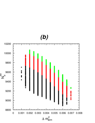
Figure 8: The total number of $\nu_{\mu}$ CC events in CNGS calculated for all points within 99% CL as a function of $\Delta m^{2}_{\rm atm}$ (a) for scheme I, (b) scheme II. The light gray/green points in (b) are with $\sin^{2}(2\theta_{\rm LSND})<0.02$ and the dark gray/red points are with $\sin^{2}(2\theta_{\rm LSND})<0.08$. The plot is for $2\times 10^{25}$ pot or 5 years.

We again calculate the total number of events in both $\nu_{e}$ and $\nu_{\mu}$ channels after $2\cdot 10^{25}$ pot (corresponding to roughly five real years) and per kilo-ton according to (20), for all points within 99% CL. The measurement of $\nu_{\mu}$ (see Fig. 8) will not reveal any difference between the two schemes unless $\Delta m^{2}_{\rm atm}$ is well known. Or, turned around, the accuracy of $\Delta m^{2}_{\rm atm}$ obtained in the case of scheme II is much weaker than that obtained in the case of scheme I.

A large LSND angle will result in more $\nu_{e}$ appearance. For OPERA the expected sensitivity in the case of a negative search is $\sin^{2}2\theta_{\mu e}\sim 1.5\times 10^{-2}$ [54] for large $\Delta m^{2}$. The proposed sensitivity of the ICARUS detectors for large $\Delta m^{2}$ is $\sin^{2}(2\theta)>2.7\times\;10^{-3}$. This is close to the limit obtained in Sec. 2.2 thereby testing nearly the whole LSND region, if the decision to build the detector is made.

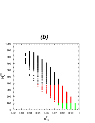
Figure 9: The total number of $\nu_{e}$ CC events in CNGS calculated for all points within 99% CL as a function $s_{13}^{2}$ (a) for scheme I, (b) for scheme II. The light gray/green points in (b) are with $\sin^{2}(2\theta_{\rm LSND})<0.02$ and the dark gray/red points are with $\sin^{2}(2\theta_{\rm LSND})<0.08$. The plot is for $2\times 10^{25}$ pot or roughly 5 years.

The total number of electron neutrinos expected at CNGS as a function of $s_{13}^{2}$ for both schemes is shown in Fig. 9. As can be seen, the conventional scheme I predicts an upper bound of $<50$ on the number of electron events observed, whereas in scheme II the number of electron events can go as high as 400 for $\sin^{2}(2\theta_{\rm LSND})=0.08$. Scheme II can thus be identified if the number of events is observed to be large, although it cannot be excluded on the basis of a low number of events observed. It is evident that the two schemes will have quite different predictions, as the LSND scheme will predict, in most of the allowed parameter space, a larger number of electron events than the conventional one. Also the energy spectrum of $\nu_{e}$ events can be seen in Fig. 10, using the same four points as in the K2K case above are shown. The energy dependence is also quite different. Hence we find that the CNGS experiments should be able to characterize the mass pattern.

The MINOS experiment [30] will have features quite similar to those of the CNGS experiments. The baseline is the same, but the mean energy is lower (around 2 GeV). Therefore it will be harder to see any difference between the two schemes, again because of the dominance of the atmospheric mass squared oscillation. The total number of electron neutrino events is expected to be similar, with a maximum of 20 for scheme I and 28 for scheme II (calculated per kilo-ton and per year). In Fig. 11 we plot the energy spectrum of the electron neutrino events with a pure $\nu_{\mu}$ beam. It is seen that only in the case of a very large LSND angle will the experiment be able to get signs for an LSND mass squared difference. In order for MINOS to be able to distinguish between the schemes, the medium or high energy option needs to be employed. Nevertheless the fact that the oscillation driven by the atmospheric mass squared difference is dominant allows an accurate determination of $\Delta m^{2}_{\rm atm}$, contrary to the CNGS experiments.

4 Summary

We explore the three-neutrino mixing scheme for solving the atmospheric and LSND anomalies, taking into account the constraints from CHOOZ. If the solar neutrino anomaly can be accounted for by some exotic mechanism, this scheme can explain all the observed neutrino experiments.

In order to check how well the atmospheric and LSND data can be explained by a three-neutrino mixing scheme, we construct a $\chi^{2}$ function that takes into account the sub-GeV and multi-GeV electron and muon events observed at SK, the $\overline{\nu}_{\mu}\to\overline{\nu}_{e}$ conversion probability observed at LSND, and the $\nu_{e}$ survival probability observed at CHOOZ. We obtain a good fit, with $\chi^{2}/{\rm dof}\approx 1$. In order to compare this goodness of fit with that of the conventional fit to the solar, atmospheric and CHOOZ data, we also construct a $\chi^{2}$ function for the conventional scheme (I). We reproduce the features of the standard three-neutrino fits, with $\chi^{2}/{\rm dof}\approx 1$. The two fits are thus equally good: the “goodness of fit” criterion, as quantified by $\chi^{2}/{\rm dof}$, by itself does not favour either of these two schemes. It is therefore necessary to investigate the often ignored scheme (II) which accounts for the atmospheric, LSND and CHOOZ data with three-neutrino oscillations.

We note some salient features of scheme II. The three-neutrino oscillation does provide a modest improvement of the fit with respect to the two-neutrino schemes. Large values of the LSND angles are favoured, with $\sin^{2}(2\theta_{\rm LSND})\simeq 0.05$, even when including the Bugey data. There are almost no matter effects in this scheme, since the values of the $\Delta m^{2}$’s are too large for the Earth’s densities to have any effect.

The two schemes differ in certain respects, which may be exploited for distinguishing between them. The ratios observed in the atmospheric neutrinos, for example, should display different behaviour. A clear signal for scheme II would be an excess of down-going multi-GeV electron neutrinos, accompanied by a small deficit for the down-going multi-GeV muon neutrinos. Also the sign of the up/down asymmetry for electron neutrino ratios is negative in the favoured region of parameter space, whereas it is positive in the conventional scheme. The current data, however, are insufficient to pick out one scheme over the other.

We also investigate the capability of the long baseline experiments — K2K, MINOS, CNGS — to distinguish between the two schemes. We compute the $\nu_{e}$ and $\nu_{\mu}$ spectra at these three experiments and find that for K2K and MINOS, the $L/E$ value is too large and the statistics too small to observe any appreciable difference. However, the final spectra at CNGS predicted by these two schemes are very different. We find that the observation of the final $\nu_{\mu}$ spectrum, as well as the $\nu_{\tau}$ appearance events that may be observed at CNGS, will not give us much useful information regarding the choice of the scheme. The apparance of $\nu_{e}$, however, can show some differences in principle, being large in scheme II. The observation of a large number of $\nu_{e}$ events can rule out the conventional scheme, although a low number of events cannot exclude scheme II.

Scheme II often gets a negatively biased treatment compared with the conventional one, mainly because it tries to explain the LSND results, which are not confirmed yet by any other experiment. As we have shown in this paper, the goodness of fit cannot be reason to prefer one scheme over the other. The ultimate arbiter of the issue is of course the experiment. The BooNE experiment will be testing the whole LSND region. With MiniBooNE proposed to be fully operative by fall 2002, it will be the first to confirm or refute the LSND results. If the LSND result is confirmed, the other experimental observations will have to be interpreted in terms of scheme II.

Acknowledgement
The authors thanks D. Harris and M. Messier for information on MINOS and K. Nakamura for information on K2K. We are indebted to P. Hernandez and A. Romanino for useful conversations. S.S. is grateful to C. Peña-Garay for valuable discussions. S.S. would like to thank the CERN theory group, where most of this work was done, for their kind hospitality. The work of S.S. was supported by NorFA, under the reference number 99.30.131-O.

Figure 1: The allowed region in the conventional case. (a) for the parameters $\Delta m^{2}_{\rm atm}$ and $4U_{\mu 3}^{2}U_{\tau 3}^{2}\simeq\sin^{2}(2\theta_{\rm atm})$ with 90% (99%) CL marked with a $\bullet$ ($\cdot$); (b) for the parameters $s_{13}^{2}$ and $s_{23}^{2}$, with 90% (99%) CL marked by a + ($\stackrel{{\scriptstyle}}{{*}}$). We have used CHOOZ and SK atmospheric data and fitted with four parameters.

Figure 2: Allowed region in $\Delta m^{2}_{\rm atm}$ and $s_{23}^{2}$ for the conventional case. In both figures the + ($+\!\!\!\!\!\!\>{\times}$) indicates points within 99% (90%) CL. (a) for all other parameters unconstrained; (b) with $\Delta m_{21}^{2}=2\times 10^{-4}$. We have used CHOOZ and SK atmospheric data and fitted with four parameters.

Figure 3: The allowed region in $s_{13}^{2}$ and $s_{23}^{2}$ for scheme I for $\Delta m^{2}_{\odot}$ constrained to (a) $2\times 10^{-4}$ and (b) $2\times 10^{-5}$. We have used CHOOZ and SK atmospheric data and fitted with four parameters.

Figure 4: Allowed region for scheme II in (a) $\Delta m^{2}_{\rm atm}$ and $4U_{\mu 1}^{2}U_{\mu 2}^{2}\simeq\sin^{2}(2\theta_{\rm atm})$ and (b) $4U_{e3}^{2}(1-U_{e3})^{2}\simeq\sin^{2}(2\theta_{\rm CHOOZ})$ and $4U_{e3}^{2}U_{\mu 3}^{2}\simeq\sin^{2}(2\theta_{LSND})$. Points within 90% (99%) CL are marked by a $\bullet$ ($\large{\cdot}$). We have used CHOOZ and SK atmospheric data and fitted with four parameters.

Figure 5: Allowed region in scheme II for parameters $s_{12}^{2}$ and $s_{23}^{2}$. Points within 68% (90%, 99%) CL are marked by $\bullet$ ($+\!\!\!\!\!\!\>{\times}$,+). We have included the LSND, CHOOZ and SK atmospheric data and fitted with four parameters.

Figure 6: Ratios as a function of the zenith angle for three best-fit points for (a) sub-GeV and (b) multi-GeV. The long-dashed curve is for scheme I constrained to $\Delta m^{2}_{\odot}=2\times 10^{-4}$. The solid curve is for scheme I constrained to $\Delta m^{2}_{\odot}=2\times 10^{-5}$. The short-dashed curve is for scheme II. Upper curves are electron neutrino ratios and lower curves are muon neutrino ratios.

Line type	$s_{12}^{2}$	$s_{23}^{2}$	$s_{13}^{2}$	$\Delta m_{31}^{2}$	$\Delta m_{21}^{2}$
Long-dashed	0.10	0.20	0.99	1.0	0.003
Short-Dashed	0.98	0.74	0.97	0.22	0.003
Dotted	0.3	0.4	0.03	0.004	0.0002
Dot-dashed	0.3	0.4	0.01	0.004	0.0002

Figure 7: The expected number of electron and muon events in the K2K experiment as a function of the neutrino energy. The solid curve corresponds to no oscillations in the muon event plot. The plot is for $10^{20}$ pot or roughly 3 years.

 

     

Line type	$s_{12}^{2}$	$s_{23}^{2}$	$s_{13}^{2}$	$\Delta m_{31}^{2}$	$\Delta m_{21}^{2}$
Long-dashed	0.10	0.20	0.99	1.0	0.003
Short-Dashed	0.98	0.74	0.97	0.22	0.003
Dotted	0.3	0.4	0.03	0.004	0.0002
Dot-dashed	0.3	0.4	0.01	0.004	0.0002

Figure 10: The expected number of electron CC events in the CERN to GRAN Sasso experiment as a function of the neutrino energy. The plot is for $2\times 10^{25}$ pot or roughly 5 years.

Line type	$s_{12}^{2}$	$s_{23}^{2}$	$s_{13}^{2}$	$\Delta m_{31}^{2}$	$\Delta m_{21}^{2}$
Long-dashed	0.10	0.20	0.99	1.0	0.003
Short-Dashed	0.98	0.74	0.97	0.22	0.003
Dotted	0.3	0.4	0.03	0.004	0.0002
Dot-dashed	0.3	0.4	0.01	0.004	0.0002

Figure 11: The expected number of electron CC events in the MINOS experiment as a function of the neutrino energy.

References

- [1] The SuperKamiokande Collaboration, Phys. Rev. Lett. 81 1562 (1998). S. Fukuda et al. [Super-Kamiokande Collaboration], Phys. Rev. Lett. 85 3999 (2000) [hep-ex/0009001].
- [2] The SuperKamiokande Collaboration, Phys.Rev.Lett. 81 1158 (1998); Erratum-ibid. 81 4279 (1998). S. Fukuda et al. [Super-Kamiokande Collaboration], hep-ex/0103033.
- [3] B.T. Cleveland et al., Astrophys.J. 496, 505 (1998); B.T. Cleveland et al., Nucl.Phys.B (Proc. Suppl.) 38, 47 (1995); R. Davis, Prog.Part.Nucl.Phys. 32, 13 (1994).
- [4] SAGE Collaboration, V. Gavrin et al., in Neutrino 96, Proc. XVII Int. Conf. on Neutrino Physics and Astrophysics, Helsinki, edited by K.Huitu, K.Enquist and J. Maalampi (World Scientific, Singapore, 1997), p. 14. V.Gavrin et al., in Neutrino 98, Proc. XVIII Int. Conf.on Neutrino Physics and Astrophysics, Takayama, Japan, 1998, edited by Y. Suzuki and Y. Totsuka.
- [5] GALLEX Collaboration, P. Anselmann et al., Phys.Lett. B342, 440 (1995); GALLEX Collaboration, W. Hampel et al., Phys.Lett. B388, 364 (1996).
- [6] C. Athanassopoulos et al. (LSND Collaboration). Phys.Rev.Lett. 81, 1774,(1998).
- [7] A. Aguilar et al. (LSND Collaboration), hep-ex/0104049.
- [8] K. Eitel (KARMEN collaboration), Nucl.Phys.Proc.Suppl. 91, 191 (2000).
- [9] K. Eitel, New Jour. Phys. 2, 1 (2000) [hep-ex/9909036].
- [10] M. Apollonio et al. [CHOOZ Collaboration], Phys.Lett.B466, 415 (1999).
- [11] B. Achkar et al., Nucl. Phys.B434, 503 (1995).
- [12] A. Bazarko (MiniBooNE Collaboration), hep-ex/0009056.
- [13] D.O. Caldwell and R.N. Mohapatra, Phys. Rev. D 48 (1993) 3259; J. Peltoniemi and J.W.F. Valle, Nucl. Phys. B 406 (1993) 409.
- [14] H. Nunokawa, hep-ph/0105027.
- [15] M.C. Gonzalez-Garcia, M. Maltoni, C.Peña-Garay, hep-ph/0105269.
- [16] M.M. Guzzo, A. Masiero, S.T. Petcov, Phys.Lett. B260, 154 (1991);
- [17] S. Bergmann, M.M. Guzzo, P.C. de Holanda, P.I. Krastev, H. Nunokawa, Phys.Rev.D62, 073001 (2000).
- [18] G. Dvali, A.Yu. Smirnov, Nucl.Phys. B563 63 (1999).
- [19] A. Lukas, P. Ramond, A. Romanino, G.G. Ross, Phys.Lett. B495 136 (2000). D.O. Caldwell, R.N. Mohapatra, S. Yellin, hep-ph/0102279. A.S. Dighe, A.S. Joshipura, hep-ph/0105288.
-
[20]
C.S. Lin, W.J. Marciano, Phys.Rev. D37, 1368 (1988).
E.Kh. Akhmedov, Sov.J.Nucl.Phys. 48, 382 (1988).
E.Kh. Akhmedov, Phys,Lett B213 (1988) 64. For a review see, E.Kh. Akhmedov, The neutrino magnetic moment and time variations of the solar neutrino flux, Preprint IC/97/49, Invited talk given at the 4th Int. Solar Neutrino Conf., Heidelberg, Germany, 1997. - [21] O.G. Miranda, C. Peña-Garay, T.I. Rashba, V.B. Semikoz, J.W.F. Valle Nucl.Phys. B595 360 (2001).
-
[22]
A. Bueno, M. Campanelli, M. Laveder, J. Rico, A. Rubbia, hep-ph/0010308;
S. Bergmann, H.V. Klapdor-Kleingrothaus, H. Päs, Phys.Rev. D62 113002 (2000). - [23] S. M. Bilenky, C. Giunti, W. Grimus and T. Schwetz, Phys. Rev. D 60 073007 (1999). O.L.G. Peres, A.Yu. Smirnov, Nucl.Phys. B599 3 (2001).
- [24] W. Grimus, T. Schwetz, hep-ph/0102252.
-
[25]
T. Teshima, T. Sakai,Phys.Rev. D62 113010 (2000);
G.L. Fogli, E. Lisi, A. Marrone, G. Scioscia, Phys.Rev. D59 033001 (1999);
O. Yasuda, Phys.Rev. D58 091301 (1998);
C. Giunti, C.W. Kim, M. Monteno, Nucl.Phys. B521, 3 (1998);
G.L. Fogli,E. Lisi,D. Montanino,G. Scioscia, Phys.Rev. D55 4385 (1997); - [26] M.C. Gonzalez-Garcia, M. Maltoni, C.Peña-Garay, J.W.F. Valle, Phys.Rev. D63, 033005 (2001).
-
[27]
V. Barger, K. Whisnant, Phys.Rev. D59 093007 (1999);
G.L. Fogli, E. Lisi, A. Marrone, D. Montanino, A. Palazzo, hep-ph/0104221. - [28] S.Choubey, S.Goswani, K.Kar, hep-ph/0004100.
-
[29]
K2K Collaboration, hep-ex/0103001.
S. Boyd, talk given at the Sixth Int. Workshop on Tau Lepton Physics, Victoria, BC, Canada, Nucl.Phys.Proc.Suppl. 98, 175 (2001); K. Nakamura, Talk presented at Neutrino-2000, Subury, Canada (http://nu2000.sno.laurentian.ca). - [30] P. Adamson et al., Fermilab report NUMI-L-337.
- [31] G. Acquistapace et al., CERN 98-02.
- [32] D.E. Groom et al., Euro.Phys.Jour. C15, 1 (2000).
- [33] G.L. Fogli, E. Lisi, A. Marrone, hep-ph/0105139.
- [34] H.Sobel (for SuperKamiokande Collaboration). Talk presented at Neutrino-2000, Sudbury, Canada (http://nu2000.sno.laurentian.ca).
-
[35]
Kamiokande Collaboration, Y. Fukuda et al.,
Phys.Lett B335, 237 (1994);
IMB Collaboration, D. Casper et al., Phys. Rev. Lett 66, 2561 (1991);
Soudan 2 Collaboration, W.W.M. Allison et al., Phys.Lett B391, 491 (1997);
NUSEX Collaboration, M. Agliette et al., Europhys. Lett 8, 611 (1989);
Frejus Collaboration, Ch. Berger et al., Phys. Lett. B227, 489 (1989);
MACRO Collaboration, M Ambrosio et al., hep-ex/9807005. - [36] T.K. Gaisser, J.S. O’Connell, Phys.Rev. D34 822 (1986).
- [37] M. Honda, Kajita, K. Kasahara, S. Midorikawa, Phys.Rev. D52, 4985 (1995).
- [38] M.C. Gonzalez-Garcia, H. Nunokawa, O.L.G. Peres, J.W.F. Valle, Nucl.Phys.B543, 3 (1999).
- [39] P. Lipari, M. Lusignoli, F. Sartogo. Phys.Rev.Lett. 74, 4384 (1995).
- [40] V. Agrawal, T.K. Gaisser, P. Lipari, T. Stanev, Phys.Rev. D53, 1314 (1996).
- [41] O.L.G. Peres, A.V. Smirnov, Phys.Lett. B456 204 (1999).
- [42] H.W. Zaglauer, K.H. Schwarzer, Z.Phys. C40, 273 (1988).
- [43] Kamiokande Collaboration, Y. Fukuda et al., Phys. Rev. Lett.77, 1683 (1996).
- [44] A.De Rujula, M.B. Gavela, P. Hernandez, hep-ph/0001124.
-
[45]
V. Plyaskin, hep-ph/0103286;
G. Fiorentini, V. Naumov and F. Villante, hep-ph/0103322. - [46] J.N. Bahcall, P.I. Krastev, A.Yu. Smirnov, hep-ph/0103179.
-
[47]
R.P. Thun, S. Mckee, Phys.Lett.B 439, 123 (1998).
G. Barenboim, F. Scheck,Phys.Lett.B440, 332 (1998).
G. Conforto, M. Barone, C. Grimani,Phys.Lett. B447, 122 (1999). - [48] G.L. Fogli, E. Lisi, A. Marrone, G. Scioscia, hep-ph/9906450.
- [49] G. Ahuja, M. Randhawa, M. Gupta, hep-ph/0104190.
- [50] H. Schlattl, hep-ph/0102063.
- [51] E. Kh. Akhmedov, A. Dighe, P. Lipari, A. Yu. Smirnov, Nucl.Phys. B542, 3 (1999).
- [52] Y. Oyama, hep-ex/0004015. Talk at XXXV Rencontres de Moriond, Les Arcs, Savoie, France, March 11-18,2000.
- [53] J.P. Revol el. al, ICARUS-TM-97/01.
- [54] K. Kodama et al., CERN/SPSC 99-20, SPSC/M635, LNGS-LOI 19/99.