[

May 2001 DPNU-01-09
Fate of Vector Dominance in the Effective Field Theory

Abstract

We reveal the full phase structure of the effective field theory for QCD, based on the hidden local symmetry (HLS) through the one-loop renormalization group equation including quadratic divergences. We then show that vector dominance (VD) is not a sacred discipline of the effective field theory but rather an accidental phenomenon peculiar to three-flavored QCD. In particular, the chiral symmetry restoration in HLS model takes place in a wide phase boundary surface, on which the VD is realized nowhere. This suggests that VD may not be valid for chiral symmetry restoration in hot and/or dense QCD.

]

Since Sakurai advocated Vector Dominance (VD) as well as vector meson universality [1], VD has been a widely accepted notion in describing vector meson phenomena in hadron physics. In fact several models such as the gauged sigma model [2] are based on VD to introduce the photon field into the Lagrangian. Moreover, it is often taken for granted in analysing the dilepton spectra to probe the phase of quark-gluon plasma for the hot and/or dense QCD [3].

As far as the well-established hadron physics for the $N_{f}=3$ case is concerned, it in fact has been extremely successful in many processes such as the electromagnetic form factor of the pion [1] and the electromagnetic $\pi\gamma$ transition form factor (See, e.g., Ref. [4].), etc. However, there has been no theoretical justification for VD and as it stands might be no more than a mnemonic useful only for the three-flavored QCD at zero temperature/density. Actually, VD is already violated for the three-flavored QCD for the anomalous processes such as $\gamma\rightarrow 3\pi/\pi^{0}\rightarrow 2\gamma$ [5, 6, 7] and $\omega\pi$ transition form factor (See, e.g., Ref. [8].). This strongly suggests that VD may not be a sacred discipline of hadron physics but may largely be violated in the different parameter space than the ordinary three-flavored QCD (non-anomalous processes) such as in the large $N_{f}$ QCD, $N_{f}$ being number of massless flavors, and hot and/or dense QCD where the chiral symmetry restoration is expected to occur. It is rather crucial whether or not VD is still valid when probing such a chiral symmetry restoration through vector meson properties [9, 10].

Here we emphasize that in the Hidden Local Symmetry (HLS) model [11, 6] the vector mesons are formulated precisely as gauge bosons; nevertheless VD as well as the universality is merely a dynamical consequence characterized by the parameter choice $a=2$.

In this paper we reveal the full phase structure of the effective field theory including the vector mesons, based on the one-loop Renormalization Group Equation (RGE) of HLS model. It turns out that in view of the phase diagram VD is very accidentally realized and only for $N_{f}=3$ QCD. On the other hand, we find a wide phase boundary surface of chiral symmetry restoration in HLS model, on which the VD is realized nowhere. Furthermore, only a single point of the phase boundary is shown to be selected by QCD through the Wilsonian matching [12], which actually coincides with the Vector Manifestation (VM) [13] realized for large $N_{f}$ QCD where VD is badly violated with $a=1$.

Let us first describe the HLS model based on the $G_{\rm global}\times H_{\rm local}$ symmetry, where $G=\mbox{SU($N_{f}$)}_{\rm L}\times\mbox{SU($N_{f}$)}_{\rm R}$ is the global chiral symmetry and $H=\mbox{SU($N_{f}$)}_{\rm V}$ is the HLS. The basic quantities are the gauge bosons $\rho_{\mu}=\rho_{\mu}^{a}T_{a}$ of the HLS and two SU($N_{f}$)-matrix valued variables $\xi_{\rm L}$ and $\xi_{\rm R}$. They are parametrized as $\xi_{\rm L,R}=e^{i\sigma/F_{\sigma}}e^{\mp i\pi/F_{\pi}}$, where $\pi=\pi^{a}T_{a}$ denotes the pseudoscalar Nambu-Goldstone (NG) bosons associated with the spontaneous breaking of $G$ and $\sigma=\sigma^{a}T_{a}$ the NG bosons absorbed into the HLS gauge bosons $\rho_{\mu}$ which is identified with the vector mesons. $F_{\pi}$ and $F_{\sigma}$ are relevant decay constants, and the parameter $a$ is defined as $a\equiv F_{\sigma}^{2}/F_{\pi}^{2}$. $\xi_{\rm L}$ and $\xi_{\rm R}$ transform as $\xi_{\rm L,R}(x)\rightarrow h(x)\xi_{\rm L,R}(x)g^{{\dagger}}_{\rm L,R}$, where $h(x)\in H_{\rm local}$ and $g_{\rm L,R}\in G_{\rm global}$. The covariant derivatives of $\xi_{\rm L,R}$ are defined by $D_{\mu}\xi_{\rm L}=\partial_{\mu}\xi_{\rm L}-ig\rho_{\mu}\xi_{\rm L}+i\xi_{\rm L}{\cal L}_{\mu}$, and similarly with replacement ${\rm L}\leftrightarrow{\rm R}$, ${\cal L}_{\mu}\leftrightarrow{\cal R}_{\mu}$, where $g$ is the HLS gauge coupling, and ${\cal L}_{\mu}$ and ${\cal R}_{\mu}$ denote the external gauge fields gauging the $G_{\rm global}$ symmetry.

The HLS Lagrangian is given by [11, 6]

$${\cal L}=F_{\pi}^{2}\,\mbox{tr}\left[\hat{\alpha}_{\perp\mu}\hat{\alpha}_{\perp}^{\mu}\right]+F_{\sigma}^{2}\,\mbox{tr}\left[\hat{\alpha}_{\parallel\mu}\hat{\alpha}_{\parallel}^{\mu}\right]+{\cal L}_{\rm kin}(\rho_{\mu})\ ,$$ (1)

where ${\cal L}_{\rm kin}(\rho_{\mu})$ denotes the kinetic term of $\rho_{\mu}$ and

$$\hat{\alpha}_{\stackrel{{\scriptstyle\perp}}{{\scriptscriptstyle\parallel}}}^{\mu}=\left(D_{\mu}\xi_{\rm R}\cdot\xi_{\rm R}^{\dagger}\mp D_{\mu}\xi_{\rm L}\cdot\xi_{\rm L}^{\dagger}\right)/(2i)\ .$$ (2)

By taking the unitary gauge, $\xi_{\rm L}^{\dagger}=\xi_{\rm R}$ ($\sigma=0$), the Lagrangian in Eq. (1) gives the following tree level relations for the vector meson mass $m_{\rho}$, the $\rho$-$\gamma$ transition strength $g_{\rho}$, the $\rho\pi\pi$ coupling constant $g_{\rho\pi\pi}$ and the direct $\gamma\pi\pi$ coupling constant $g_{\gamma\pi\pi}$: [11, 6]

$$m_{\rho}^{2}=ag^{2}F_{\pi}^{2}\ ,\quad g_{\rho\pi\pi}=\frac{1}{2}ag\ ,$$ (3)

$$g_{\rho}=agF_{\pi}^{2}\ ,\quad g_{\gamma\pi\pi}=\left(1-\frac{a}{2}\right)e\ ,$$ (4)

where $e$ is the electromagnetic coupling constant.

Expressions for $g_{\rho\pi\pi}$ and $g_{\rho}$ in Eq. (4) lead to the celebrated Kawarabayashi-Suzuki-Riazuddin-Fayyazuddin (KSRF) relation [14] (version I)

$$g_{\rho}=2F_{\pi}^{2}g_{\rho\pi\pi}\ ,$$ (5)

independently of the parameter $a$. This is the low energy theorem of the HLS [15], which was proved at one-loop [16], and then at any loop order [17]. On the other hand, making a dynamical assumption of a parameter choice $a=2$, the following outstanding phenomenological facts are reproduced from Eq. (4): [11, 6]

1. $g_{\rho\pi\pi}=g$ (universality of the $\rho$-coupling) [1]

2. $m_{\rho}^{2}=2g_{\rho\pi\pi}^{2}F_{\pi}^{2}$ (KSRF II) [14]

3. $g_{\gamma\pi\pi}=0$ (vector dominance of the electromagnetic form factor of the $\pi$) [1]

Thus, even though the vector mesons are gauge bosons in the HLS model, VD as well as the universality is not automatic consequence but rather dynamical one of a parameter choice of $a=2$.

Actually, due to quantum corrections the parameters change their values by the energy scale, which are determined by the RGE’s. Accordingly, values of the parameters $F_{\pi}$, $a$ and $g$ cannot be freely chosen, although they are independent at tree level. Thus, we first study the RG flows of the parameters and the phase structure of the HLS to classify the parameter space. Here we stress that thanks to the gauge symmetry in the HLS model it is possible to perform a systematic loop expansion including the vector mesons in addition to the pseudoscalar mesons [18, 16, 19, 12, 7] in a way to extend the chiral perturbation theory [20]. There the loop expansion corresponds to the derivative expansion, so that the one-loop calculation of the RGE is reliable in the low energy region.

As shown in Ref. [21, 12] it is important to include quadratic divergences in calculating the quantum corrections. Due to quadratic divergences in the HLS dynamics, it follows that even if the bare theory defined by the cutoff $\Lambda$ is written as if it were in the broken phase characterized by $F_{\pi}^{2}(\Lambda)>0$, the quantum theory can be in the symmetric phase characterized by $F_{\pi}^{2}(0)=0$ [21]. The one-loop RGE’s for $F_{\pi}$, $a$ and $g$ including quadratic divergences are given by [21, 12]

$$\mu\frac{dF_{\pi}^{2}}{d\mu}=C\left[3a^{2}g^{2}F_{\pi}^{2}+2(2-a)\mu^{2}\right]\ ,$$ (6)

$$\mu\frac{da}{d\mu}=-C(a-1)\left[3a(a+1)g^{2}-(3a-1)\frac{\mu^{2}}{F_{\pi}^{2}}\right]\ ,$$ (7)

$$\mu\frac{dg^{2}}{d\mu}=-C\frac{87-a^{2}}{6}g^{4}\ .$$ (8)

where $C=N_{f}/\left[2(4\pi)^{2}\right]$ and $\mu$ is the renormalization scale. It is convenient to use the following quantities:

$$X(\mu)\equiv C\mu^{2}/F_{\pi}^{2}(\mu)\ ,\quad G(\mu)\equiv Cg^{2}(\mu)\ .$$ (9)

Then, the RGE’s in Eq. (8) are rewritten as

$$\mu\frac{dX}{d\mu}=(2-3a^{2}G)X-2(2-a)X^{2}\ ,$$ (10)

$$\mu\frac{da}{d\mu}=-(a-1)\left[3a(a+1)G-(3a-1)X\right]\ ,$$ (11)

$$\mu\frac{dG}{d\mu}=-\frac{87-a^{2}}{6}G^{2}\ .$$ (12)

It should be noticed that the RGE’s in Eq. (12) are valid above the $\rho$ mass scale $m_{\rho}$, where $m_{\rho}$ is defined by the on-shell condition $m_{\rho}^{2}=a(m_{\rho})g^{2}(m_{\rho})F_{\pi}^{2}(m_{\rho})$. In terms of $X$, $a$ and $G$, the on-shell condition becomes $a(m_{\rho})G(m_{\rho})=X(m_{\rho})$. Then the region where the RGE’s in Eq. (12) are valid is specified by the condition $a(\mu)G(\mu)\leq X(\mu)$.

Seeking the parameters for which all right-hand-sides of three RGE’s in Eq. (12) vanish simultaneously, we obtain three fixed points and one fixed line in the physical region and one fixed point in the unphysical region (i.e., $a<0$ and $X<0$). Those in the physical region (labeled by $i=1,\ldots,4$) are given by

$$\left(X^{\ast}_{i},\,a^{\ast}_{i},\,G^{\ast}_{i}\right)=\left(0,\,\mbox{any},\,0\right)\ ,\quad\left(1,\,1,\,0\right)\ ,\quad\left(\frac{3}{5},\,\frac{1}{3},\,0\right)\ ,$$ (13)

$$\quad\left(\frac{2(2+45\sqrt{87})}{4097},\,\sqrt{87},\,\frac{2(11919-176\sqrt{87})}{1069317}\right)\ .$$ (14)

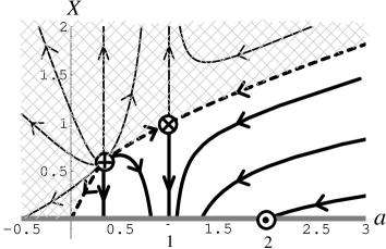
FIG. 1.: Phase diagram on $G=0$ plane. Arrows on the flows are written from the ultraviolet to the infrared. Gray line denotes the fixed line $(X^{\ast}_{1},a^{\ast}_{1},G^{\ast}_{1})=(0,\mbox{any},0)$. Points indicated by $\oplus$ and $\otimes$ (VM point) denote the fixed points $(3/5,1/3,0)$ and $(1,1,0)$, respectively. Dashed lines divide the broken phase (lower side) and the symmetric phase (upper side; cross-hatched area): Flows drawn by thick lines are in the broken phase, while those by thin lines are in the symmetric phase. The point indicated by $\odot$, $(X,a,G)=(0,2,0)$, correspond to the VD, $a(0)=2$.

Note that $G=0$ is a fixed point of the RGE for $G$, and $a=1$ is the one for $a$. Hence RG flows on $G=0$ plane and $a=1$ plane are confined in the respective planes.

Let us first study the phase structure of the HLS for $G=0$ (see Fig. 1) in which case $m_{\rho}$ vanishes and the RGE’s (12) are valid all the way down to the low energy limit, $\mu\geq m_{\rho}=0$. There are one fixed line and two fixed points [first three in Eq. (14)]. Generally, the phase boundary is specified by $F_{\pi}^{2}(0)=0$, namely, governed by the infrared fixed point such that $X(0)\neq 0$ (see Eq. (9)). Such a fixed point is the point $(X^{\ast}_{2},a^{\ast}_{2},G^{\ast}_{2})=(1,1,0)$, which is nothing but the VM point [13]. Then the phase boundary is given by the RG flows entering $(X^{\ast}_{2},a^{\ast}_{2},G^{\ast}_{2})$. Since $a=1/3$ is a fixed point of the RGE for $a$ in Eq. (12), the RG flows for $a<1/3$ cannot enter $(X^{\ast}_{2},a^{\ast}_{2},G^{\ast}_{2})$. Hence there is no phase boundary specified by $F_{\pi}^{2}(0)=0$ in $a<1/3$ region. Instead, $F_{\sigma}^{2}(0)$ vanishes even though $F_{\pi}^{2}(0)\neq 0$, namely $a(0)=X(0)=0$. Then the phase boundary for $a<1/3$ is given by the RG flow entering the point $(X,a,G)=(0,0,0)$. In Fig. 1 the phase boundary is drawn by the dashed line, which divides the phases into the symmetric phase [22] (upper side; cross-hatched area) and the broken one (lower side).

In the case of $G>0$, on the other hand, the $\rho$ becomes massive ($m_{\rho}\neq 0$), and thus decouples at $m_{\rho}$ scale. Below the $m_{\rho}$ scale $a$ and $G$ no longer run, while $F_{\pi}$ still runs by the $\pi$ loop effect. Thus, to study the phase structure for $G>0$ we need the RGE for $F_{\pi}$ for $\mu<m_{\rho}$ (denoted by $F_{\pi}^{(\pi)}$). This is given by $d[F_{\pi}^{(\pi)}]^{2}/d\mu^{2}=2C$ [21], which is readily solved as

$$\left[F_{\pi}^{(\pi)}(\mu)\right]^{2}=\left[F_{\pi}^{(\pi)}(m_{\rho})\right]^{2}-2C\left(m_{\rho}^{2}-\mu^{2}\right)\ .$$ (15)

Then the quadratic divergence (second term in Eq. (15)) of the $\pi$ loop can give rise to chiral symmetry restoration $F_{\pi}^{(\pi)}(0)=0$ [21]. Thus the phase boundary is specified by the condition $[F_{\pi}^{(\pi)}(m_{\rho})]^{2}=2Cm_{\rho}^{2}$. Note that the relation between $[F_{\pi}^{(\pi)}(m_{\rho})]^{2}$ and $F_{\pi}^{2}(m_{\rho})$ including the finite renormalization effect is given by [12]

$$\left[F_{\pi}^{(\pi)}(m_{\rho})\right]^{2}=F_{\pi}^{2}(m_{\rho})+C\,a(m_{\rho})m_{\rho}^{2}\ ,$$ (16)

which is converted into the condition for $X(m_{\rho})$ and $a(m_{\rho})$. Combination of this with the on-shell condition specifies the phase boundary in the full $(X,a,G)$ space, which is given by the collection of the RG flows entering points on the line specified by

$$2-a(m_{\rho})=1/X(m_{\rho})\ ,$$ (17)

$$a(m_{\rho})G(m_{\rho})=X(m_{\rho})\ .$$ (18)

Such a surface can be imagined from Figs. 1 and 2.

We now study the $a=1$ plane (see Fig. 2). The flows stop at the on-shell of $\rho$ ($G=X$; dot-dashed line in Fig. 2) and should be switched over to RGE of $F_{\pi}^{(\pi)}(\mu)$ as mentioned above. From Eq. (18) with $a=1$ the flow entering $(X,G)=(1,1)$ (dashed line) is the phase boundary which distinguishes the broken phase (lower side) from the symmetric one (upper side; cross-hatched area).

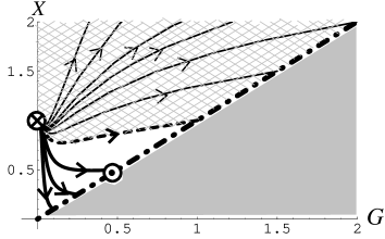
FIG. 2.: Phase diagram on $a=1$ plane. Arrows on the flows are written from the ultraviolet to the infrared. Point indicated by $\otimes$ denotes the VM fixed point $(X^{\ast}_{2},a^{\ast}_{2},G^{\ast}_{2})=\left(1,1,0\right)$. Flows drawn by thick lines are in the broken phase, while those by thin lines are in the symmetric phase (cross-hatched area). Dot-dashed line corresponds to the on-shell condition $G=X$. In the shaded area the RGE’s (12) are not valid since $\rho$ has already decoupled. Point indicated by $\odot$, $\left(1/2,1,1/2\right)$, corresponds to the VD, $a(0)=2$. (See Eq. (20).)

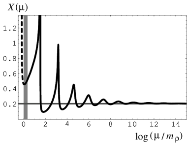
FIG. 3.: Scale dependence of $X(\mu)$ in QCD with $N_{f}=3$. Shaded area denotes the physical region, $m_{\rho}\leq\mu\leq\Lambda$. Flow shown by the dashed line are obtained by extending it to the (unphysical) infrared region by taking literally the RGE’s in Eq. (12). In an idealized high energy limit the flow approaches to the fixed point $X^{\ast}_{4}=2(2+45\sqrt{87})/4097\simeq 0.2$.

For $a<1$, RG flows approach to the fixed point $\left(X^{\ast}_{3},a^{\ast}_{3},G^{\ast}_{3}\right)=(3/5,1/3,0)$ in the idealized high energy limit ($\mu\rightarrow\infty$).

For $a>1$, RG flows in the broken phase approach to $\left(X^{\ast}_{4},a^{\ast}_{4},G^{\ast}_{4}\right)\simeq(0.2,9.3,0.02)$, which is precisely the fixed point that the RG flow of the $N_{f}=3$ QCD belongs to. To see how the RG flow of $N_{f}=3$ QCD approaches to this fixed point, we show the $\mu$-dependence of $X(\mu)$ in Fig. 3 where values of the parameters at $\mu=m_{\rho}$ are set to be $\left(X(m_{\rho}),a(m_{\rho}),G(m_{\rho})\right)\simeq\left(0.46,1.22,0.38\right)$ through Wilsonian matching with the underlying QCD [12]. The values of $X$ close to $1/2$ in the physical region ($m_{\rho}\leq\mu\leq\Lambda$) are very unstable against RGE flow, and hence $X\sim 1/2$ is realized in a very accidental way.

Let us now discuss the VD which is characterized by $a(0)=2$. Since $F_{\sigma}^{2}$ does not run for $\mu<m_{\rho}$ while $F_{\pi}^{2}$ does, we have [12]

$$a(\mu)\equiv\left\{\begin{array}[]{ll}F_{\sigma}^{2}(\mu)/F_{\pi}^{2}(\mu)&(\mu>m_{\rho})\ ,\\ F_{\sigma}^{2}(m_{\rho})/\left[F_{\pi}^{(\pi)}(\mu)\right]^{2}&(\mu<m_{\rho})\ .\end{array}\right.$$ (19)

Then by using Eqs. (15) and (16), $a(0)$ is given by

$$a(0)=a(m_{\rho})/\left[1+a(m_{\rho})X(m_{\rho})-2X(m_{\rho})\right]\ .$$ (20)

This implies that the VD ($a(0)=2$) is only realized for $(X(m_{\rho}),a(m_{\rho}))=(1/2,\mbox{any})$ or $(\mbox{any},2)$.

In $N_{f}=3$ QCD, the parameters at $m_{\rho}$ scale, $\left(X(m_{\rho}),a(m_{\rho}),G(m_{\rho})\right)\simeq\left(0.46,1.22,0.38\right)$, happen to be near such a VD point. However, the RG flow actually belongs to the fixed point $\left(X^{\ast}_{4},a^{\ast}_{4},G^{\ast}_{4}\right)$ which is far away from the VD value. Thus, the VD in $N_{f}=3$ QCD is accidentally realized by $X(m_{\rho})\sim 1/2$ which is very unstable against the RG flow (see Fig. 3). For $G=0$ (Fig. 1) the VD holds only if the parameters are (accidentally) chosen to be on the RG flow entering $\left(X,a,G\right)=\left(0,2,0\right)$ (indicated by $\odot$) which is an end point of the line $\left(X(m_{\rho}),a(m_{\rho})\right)=(\mbox{any},2)$. For $a=1$ (Fig. 2), on the other hand, the VD point $\left(X,a,G\right)=\left(1/2,1,1/2\right)$ (indicated by $\odot$) lies on the line $\left(X(m_{\rho}),a(m_{\rho})\right)=(1/2,\mbox{any})$.

Then, phase diagrams in Figs. 1 and 2 and their extensions to the entire parameter space (including Fig. 3) show that neither $X(m_{\rho})=1/2$ nor $a(m_{\rho})=2$ is a special point in the parameter space of the HLS. Thus we conclude that the VD as well as the universality can be satisfied only accidentally. Therefore, when we change the parameter of QCD, the VD is generally violated. In particular, neither $X(m_{\rho})=1/2$ nor $a(m_{\rho})=2$ is satisfied on the phase boundary surface characterized by Eq. (18) where the chiral restoration takes place in HLS model. Therefore, VD is realized nowhere on the chiral restoration surface !

Moreover, when the HLS is matched with QCD, only the point $(X^{\ast}_{2},a^{\ast}_{2},G^{\ast}_{2})=(1,1,0)$, the VM point, on the phase boundary is selected, since the axialvector and vector current correlators in HLS can be matched with those in QCD only at that point [13]. Therefore, QCD predicts $a(0)=1$, i.e., large violation of the VD at chiral restoration. Actually, for the chiral restoration in the large $N_{f}$ QCD [23, 24] the VM can in fact takes place [13], and thus the VD is badly violated.

Finally, we suggest that if the VM takes place in other chiral restoration such as the one in the hot and/or dense QCD, the VD should be largely violated near the critical point.

This work is supported in part by Grant-in-Aid for Scientific Research (B)#11695030 (K.Y.), (A)#12014206 (K.Y.) and (A)#12740144 (M.H.).

REFERENCES

- [1] See J.J. Sakurai, Currents and Mesons (University of Chicago, Chicago, 1969).
- [2] See, e.g., U. G. Meissner, Phys. Rept. 161, 213 (1988); O. Kaymakcalan, S. Rajeev and J. Schechter, Phys. Rev. D 30, 594 (1984).
- [3] See, e.g., R. D. Pisarski, Phys. Rev. D 52, R3773 (1995); F. Klingl, N. Kaiser and W. Weise, Nucl. Phys. A 624, 527 (1997); R. Rapp and J. Wambach, Adv. Nucl. Phys. 25, 1 (2000).
- [4] H. J. Behrend et al. [CELLO Collaboration], Z. Phys. C 49, 401 (1991).
- [5] T. Fujiwara, T. Kugo, H. Terao, S. Uehara and K. Yamawaki, Prog. Theor. Phys. 73, 926 (1985).
- [6] M. Bando, T. Kugo and K. Yamawaki, Phys. Rept. 164, 217 (1988).
- [7] M. Harada and K. Yamawaki, to appear in Phys. Rept.
- [8] A. Bramon, A. Grau and G. Pancheri, Phys. Lett. B 277, 353 (1992); M. Bando and M. Harada, Prog. Theor. Phys. 92, 583 (1994); Phys. Rev. D 49, 6096 (1994).
- [9] R.D. Pisarski, Phys. Lett. B 110, 155 (1982); hep-ph/9503330.
- [10] G. E. Brown and M. Rho, Phys. Rev. Lett. 66, 2720 (1991); Phys. Rept. 269, 333 (1996); nucl-th/0101015; hep-ph/0103102.
- [11] M. Bando, T. Kugo, S. Uehara, K. Yamawaki and T. Yanagida, Phys. Rev. Lett. 54, 1215 (1985).
- [12] M. Harada and K. Yamawaki, Phys. Rev. D 64, 014023 (2001).
- [13] M. Harada and K. Yamawaki, Phys. Rev. Lett. 86, 757 (2001).
- [14] K. Kawarabayashi and M. Suzuki, Phys. Rev. Lett. 16, 255 (1966): Riazuddin and Fayyazuddin, Phys. Rev. 147, 1071 (1966).
- [15] M. Bando, T. Kugo and K. Yamawaki, Nucl. Phys. B 259, 493 (1985); Prog. Theor. Phys. 73, 1541 (1985).
- [16] M. Harada and K. Yamawaki, Phys. Lett. B 297, 151 (1992).
- [17] M. Harada, T. Kugo and K. Yamawaki, Phys. Rev. Lett. 71, 1299 (1993); Prog. Theor. Phys. 91, 801 (1994).
- [18] H. Georgi, Phys. Rev. Lett. 63, 1917 (1989).
- [19] M. Tanabashi, Phys. Lett. B 316, 534 (1993).
- [20] S. Weinberg, Physica A 96, 327 (1979): J. Gasser and H. Leutwyler, Annals Phys. 158, 142 (1984).
- [21] M. Harada and K. Yamawaki, Phys. Rev. Lett. 83, 3374 (1999).
- [22] Here “symmetric phase” means that or , namely or for non-zero (finite) .
- [23] Y. Iwasaki, K. Kanaya, S. Kaya, S. Sakai and T. Yoshie, Prog. Theor. Phys. Suppl. 131, 415 (1998), and references cited therein.
- [24] T. Appelquist, J. Terning and L.C. Wijewardhana, Phys. Rev. Lett. 77, 1214 (1996).