Effective field theory for the small-$x$ evolution

I. Balitsky Physics Department, Old Dominion University, Norfolk VA 23529
and Theory Group, Jefferson Lab, Newport News VA 23606
Abstract

The small-$x$ behavior of structure functions in the saturation region is determined by the non-linear generalization of the BFKL equation. I suggest the effective field theory for the small-$x$ evolution which solves formally this equation. The result is the $2+1$ functional integral for the structure functions at small $x$.

pacs:
PACS numbers: 12.38.Bx, 11.10.Jj, 11.55.Jy

The great success of pQCD in describing the $Q^{2}$ behavior of structure functions of deep inelastic scattering (DIS) can be traced back to the fact that the $Q^{2}$ dependence is governed by DGLAP evolution equations which have two remarkable properties: they are linear equations, and the evolution at high $Q^{2}$ is purely perturbative (the non-perturbative physics enters the game only when we lower the normalization point $\mu^{2}$ down to the typical hadronic scale $\sim 1$GeV). The higher-order terms of perturbative expansion for both the coefficient functions and the anomalous dimensions of the light-cone operators lie in the same framework of linear evolution and lead to the corrections $\sim\alpha_{s},\alpha_{s}^{2}$ etc.

The situation for the small-x DIS is more complicated. In the leading logarithmic approximation (LLA) the small-x asymptotics is described by the BFKL pomeron[1]. It is possible to reformulate the BFKL equation as an evolution equation where the relevant operators are Wilson lines - infinite gauge links[2]. *** At high energies the particles move so fast that their trajectories can be approximated by straight lines collinear to their velocities. The proper degrees of freedom for the fast particles moving along the straight lines are the (infinite) gauge factors ordered along the straight line [4]. The evolution of the two-Wilson-line operator (β€œcolor dipole”) with respect to the slope of Wilson lines reproduces the BFKL equation.

Unfortunately, the theoretical status of the BFKL evolution is not as clear as the DGLAP one (for the review, see Refs. [3]). The biggest problem is the lack of unitarity: the power behavior of the BFKL cross section violates the Froissart bound and therefore, in order get the true asymptotics at small $x$, we must go beyond the LLA. At this step, we face a new problem. In the DGLAP case, the sub-leading logaritms follow the same general pattern of linear DGLAP equation and the problem is purely technical: calculating the loop corrections to the kernels. In the case of small-$x$ evolution there are also $\alpha_{s}$ corrections to the BFKL kernel[5], but, on the top of that, there are the unitarity corrections which lie outside the framework of the BFKL equation. At small $\alpha_{s}$ and $x$, these corrections seem to dominate over the NLO BFKL ones[6].

Another problem with the BFKL evolution is infrared instability. We can safely apply pQCD to the small-$x$ DIS if the characteristic transverse momenta of the gluons $k_{\perp}$ in the gluon ladder are large. For the the first few diagrams, one can check by explicit calculation that the characteristic $k^{2}_{\perp}$ are $\sim Q^{2}$. However, as $x$ decreases, it turns out that the characteristic transverse momenta in the middle of the gluon ladder drift to $\Lambda_{\rm QCD}$ making the application of pQCD questionable.

Recently, an idea has emerged that these two difficulties may cancel each other out. Consider the DIS from the heavy nuclei where the large density sets the saturation scale $Q_{s}$ [7, 8, 9, 10] which effectively cuts the integration over $k_{\perp}$ even at relatively low energy. As we shall see below, the small-$x$ evolution in this case is non-linear which leads to the growth of the saturation scale with energy, see the discussion in Refs. [7, 8, 9, 10, 11, 12]. It is natural to assume that even for the DIS from the nucleon where there is no saturation at low energies, the saturation scale at sufficiently small $x$ may be generated by the non-linear evolution itself. Indeed, the parton recombination described by the non-linear evolution must balance at some point the effects of parton splitting so the partons will reach the state of the saturation. In this high-density regime the coupling constant is small but the characteristic fields are large, making a perfect case for the application of the semiclassical QCD methods[9, 13, 14]. The high-density regime of QCD can serve as a bridge between the domain of pQCD and the β€œreal” non-perturbative QCD regime governed by the physics of confinement.

In this paper I suggest the effective field theory which describes the small-$x$ evolution in the saturation region. First, let me remind the OPE for high-energy amplitudes derived in [2]. Consider the amplitude of forward $\gamma^{*}\gamma^{*}$-scattering at small $x_{B}={Q^{2}\over s}$. In the target frame, the virtual photon splits into $q\bar{q}$ pair which approaches the nucleon at high speed. Due to the high speed the classical trajectories of the quarks are straight lines collinear to the momentum of the incoming photon $q$. The corresponding operator expansion switched between nucleon states has the form [2]:

$\displaystyle\int\!d^{4}xe^{iq\cdot x}\langle p|T\{j_{\mu}(x)j_{\nu}(0)\}|p\rangle$ (1)
=∫d2​xβŸ‚β€‹Iμ​ν​(xβŸ‚)β€‹βŸ¨p|Tr{U^​(xβŸ‚)​U^†​(0)}|p⟩,absentsuperscript𝑑2subscriptπ‘₯perpendicular-tosubscriptπΌπœ‡πœˆsubscriptπ‘₯perpendicular-toquantum-operator-product𝑝Tr^π‘ˆsubscriptπ‘₯perpendicular-tosuperscript^π‘ˆβ€ 0𝑝\displaystyle=~{}\int d^{2}x_{\perp}I_{\mu\nu}(x_{\perp})\langle p|\mathop{\rm Tr}\{\hat{U}(x_{\perp})\hat{U}^{\dagger}(0)\}|p\rangle, (2)

where $I_{\mu\nu}(x_{\perp})$ is a certain numerical function of the transverse separation of quarks $x_{\perp}$ and virtuality of the photon $Q^{2}=-q^{2}$. The relevant operators U​(U†)π‘ˆsuperscriptπ‘ˆβ€ U(U^{\dagger}) are gauge factors ordered along the classical trajectories which are almost light-like lines stretching from minus to plus infinity:

$$U(z_{\perp})=P\exp\left(i\int_{-\infty}^{\infty}due^{\mu}A_{\mu}(ue+z_{\perp})\right)$$ (3)

where $e$ is collinear to $q$ and $z_{\perp}$ is the transverse position of the Wilson line.

It turns out that the small-$x$ behavior of structure functions is governed by the evolution of these operators with respect to the deviation of the Wilson lines from the light cone; this deviation serves as a kind of β€œrenormalization point” for these operators. At infinite energy, the vector $e$ is light-like and the corresponding matrix elements of the operators (3) have a logarithmic divergence in longitudinal momenta. To regularize it , we consider operators corresponding to large but finite velocity and take $e_{\zeta}=e_{1}~{}+~{}\zeta e_{2}$ where $e_{1}=(q-\frac{q^{2}}{2pq}p)$ and $e_{2}=p$ are the lightlike vectors close to the directions of the colliding particles. Now, instead of studying the energy-dependence of the physical amplitude we must investigate the dependence of the operators (3) on the slope $\zeta$. Large energies mean small $\zeta$ and we can sum up logarithms of $\zeta$ instead of logarithms of $s$ (At present, we can do it only in the leading logarithmic approximation (LLA) $\alpha_{s}\ll 1$, $\alpha_{s}\ln{s\over m^{2}}\sim 1$). The equation governing the dependense of $U$ on $\zeta$ has the form [2] †††The first non-linear equation for parton densities is known since 1983 as the GLR equation (it was conjectured in Ref. [7] and proved in the double-log limit in Ref.Β [8]). The full LLA $x$ result was first derived in Ref. [2] by the above method. After that, it was reobtained in Ref.Β [11] in the framework of the dipole model[15, 16], in Ref. [17] by direct summation of relevant Feynman diagrams, and in Refs. [19, 20] by the semiclassical methods.

$\displaystyle\zeta\frac{d}{d\zeta}{\cal U}(x_{\perp},y_{\perp})$ (4)
$\displaystyle=$ $\displaystyle{\alpha_{s}N_{c}\over 2\pi^{2}}\int dz_{\perp}{(x_{\perp}-y_{\perp})^{2}\over(x_{\perp}-z_{\perp})^{2}(z_{\perp}-y_{\perp})^{2}}\Big{\{}{\cal U}(x_{\perp},z_{\perp})$ (5)
$\displaystyle+$ $\displaystyle{\cal U}(z_{\perp},y_{\perp})-{\cal U}(x_{\perp},y_{\perp})+{\cal U}(x_{\perp},z_{\perp}){\cal U}(z_{\perp},y_{\perp})\Big{\}}$ (6)

where 𝒰​(xβŸ‚,yβŸ‚)≑1Nc​Tr{U​(xβŸ‚)​U†​(yβŸ‚)}βˆ’1𝒰subscriptπ‘₯perpendicular-tosubscript𝑦perpendicular-to1subscript𝑁𝑐Trπ‘ˆsubscriptπ‘₯perpendicular-tosuperscriptπ‘ˆβ€ subscript𝑦perpendicular-to1{\cal U}(x_{\perp},y_{\perp})\equiv{1\over N_{c}}\mathop{\rm Tr}\{U(x_{\perp})U^{\dagger}(y_{\perp})\}-1. The first three linear terms in braces in the r.h.s. of eq. (4)) reproduces the BFKL pomeron[1] while the quadratic term will give us the three-pomeron vertex[18]. The solution of the linearized evolution equation is especially simple in the case of zero momentum transfer (e.g. for the total cross section of small-x DIS):

$\displaystyle\langle p|{\cal U}^{\zeta=x_{B}}(x_{\perp},0)|p\rangle~{}=~{}\int\!\frac{d\nu}{2\pi^{2}}(x_{\perp}^{2})^{-\frac{1}{2}+i\nu}$ (7)
$\displaystyle\left(\frac{s}{m^{2}}\right)^{\omega(\nu)}\int\!dz_{\perp}(z_{\perp}^{2})^{-\frac{1}{2}-i\nu}\langle p|{\cal U}^{\zeta_{0}}(z_{\perp},0)|p\rangle$ (8)

where ω​(Ξ½)=2​Nc​αsπ​[βˆ’ReΟˆβ€‹(12+i​ν)βˆ’C]πœ”πœˆ2subscript𝑁𝑐subscriptπ›Όπ‘ πœ‹delimited-[]Reπœ“12π‘–πœˆπΆ\omega(\nu)=2N_{c}{\alpha_{s}\over\pi}[-\mathop{\rm Re}\psi(\frac{1}{2}+i\nu)-C] and m2superscriptπ‘š2m^{2} is either Q2superscript𝑄2Q^{2} or mN2superscriptsubscriptπ‘šπ‘2m_{N}^{2} (in LLA, we cannot distinquish between Ξ±s​ln⁑sQ2subscript𝛼𝑠𝑠superscript𝑄2\alpha_{s}\ln{s\over Q^{2}} and Ξ±s​ln⁑smN2subscript𝛼𝑠𝑠superscriptsubscriptπ‘šπ‘2\alpha_{s}\ln{s\over m_{N}^{2}}). 
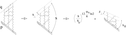
The sketch of linear evolution is presented in Fig. 1.

Refer to caption

FIG. 1.: BFKL evolution in terms of Wilson-line operators (denoted by dotted lines).

The starting point of the evolution is the slope collinear to the momentum of the incoming photon q ($\zeta=x_{B}$) and it is convenient to stop the evolution at a certain intermediate point $\zeta_{0}={Q^{2}\over s_{0}}$ where s0≫mN2,Ξ±sπ​ln⁑s0mN2β‰ͺ1formulae-sequencemuch-greater-thansubscript𝑠0superscriptsubscriptπ‘šπ‘2much-less-thansubscriptπ›Όπ‘ πœ‹subscript𝑠0superscriptsubscriptπ‘šπ‘21s_{0}\gg m_{N}^{2},~{}~{}{\alpha_{s}\over\pi}\ln{s_{0}\over m_{N}^{2}}\ll 1~{}. The first of these conditions means that $s_{0}$ is still high from the viewpoint of low-energy nucleon physics while the second condition means that $s_{0}$ is sufficiently small from the viewpoint of high-energy physics (so one can neglect the BFKL logs). The matrix element of the double-Wilson-line operator at this slope is a phenomenological input for the BFKL evolution (just as the structure function at low $Q^{2}$ serves as the input for ordinary DGLAP evolution). At large $s$ the integral over $\nu$ is dominated by the vicinity of $\nu=0$ which gives the familiar BFKL asymptotics Οƒtot≃xBβˆ’12​αsπ​ln⁑2similar-to-or-equalssuperscript𝜎totsuperscriptsubscriptπ‘₯𝐡12subscriptπ›Όπ‘ πœ‹2\sigma^{\rm tot}\simeq x_{B}^{-12{\alpha_{s}\over\pi}\ln 2}.

Unlike the linear evolution, the general picture is very complicated since the number of operators $U$ and U†superscriptπ‘ˆβ€ U^{\dagger} increases after each evolution. At the time being, it is not known how to solve the non-linear evolution equation in an explicit form. It is possible, however, to write down the solution of the non-linear equation (4) in the form of a functional integral over the double set of the variables, $\varsigma_{i=1,2}(z_{\perp},\eta)=t^{a}\varsigma_{i=1,2}^{a}(z_{\perp},\eta)$ belonging to the Lie algebra of the SU(3) color group and $\Omega_{i=1,2}(z_{\perp},\eta)$ belonging to the group itself:

UΞ·A​(xβŸ‚)βŠ—U†ηA​(yβŸ‚)=tensor-productsuperscriptπ‘ˆsubscriptπœ‚π΄subscriptπ‘₯perpendicular-tosuperscriptπ‘ˆβ€ absentsubscriptπœ‚π΄subscript𝑦perpendicular-toabsent\displaystyle U^{\eta_{A}}(x_{\perp})\otimes U^{\dagger\eta_{A}}(y_{\perp})~{}= (9)
$\displaystyle~{}\int^{\pi_{1,2}(\eta_{A})=0}_{\Omega_{1,2}(\eta_{0})=1}D\varsigma_{1}(z,\eta)D\varsigma_{2}(z,\eta)D\Omega_{1}(z,\eta)D\Omega_{2}(z,\eta)$ (10)
Ξ©1†​(xβŸ‚,Ξ·A)​UxΞ·0​Ω2​(xβŸ‚,Ξ·A)βŠ—Ξ©2†​(yβŸ‚,Ξ·A)​Uy†η0​Ω1​(yβŸ‚,Ξ·A)tensor-productsubscriptsuperscriptΩ†1subscriptπ‘₯perpendicular-tosubscriptπœ‚π΄subscriptsuperscriptπ‘ˆsubscriptπœ‚0π‘₯subscriptΞ©2subscriptπ‘₯perpendicular-tosubscriptπœ‚π΄subscriptsuperscriptΩ†2subscript𝑦perpendicular-tosubscriptπœ‚π΄subscriptsuperscriptπ‘ˆβ€ absentsubscriptπœ‚0𝑦subscriptΞ©1subscript𝑦perpendicular-tosubscriptπœ‚π΄\displaystyle\Omega^{\dagger}_{1}(x_{\perp},\eta_{A})U^{\eta_{0}}_{x}\Omega_{2}(x_{\perp},\eta_{A})\otimes\Omega^{\dagger}_{2}(y_{\perp},\eta_{A})U^{\dagger\eta_{0}}_{y}\Omega_{1}(y_{\perp},\eta_{A}) (11)
$\displaystyle~{}\exp\Bigg{\{}\int^{\eta_{A}}_{\eta_{0}}d\eta\!\int\!d^{2}z\Big{[}\frac{1}{g}\sum_{i=1,2}\varsigma_{i}^{a}(z,\eta)\vec{\partial}^{2}\Big{(}\Omega_{i}^{\dagger}(z,\eta)\dot{\Omega}_{i}(z,\eta)\Big{)}^{a}$ (12)
$\displaystyle~{}-\frac{1}{4\pi}\varsigma_{1}^{a}(z,\eta)\varsigma_{2}^{b}(z,\eta)\vec{\partial}^{2}\Big{(}\Omega_{1}^{\dagger}(z,\eta)U^{\eta_{0}}_{z}\Omega_{2}(z,\eta)\Big{)}^{ab}\Big{]}\Bigg{\}}$ (13)

where $\dot{\Omega}\equiv\frac{\partial}{\partial\eta}\Omega$ and (Ω†​Ω˙)a≑2​T​r​{ta​Ω†​Ω˙}superscriptsuperscriptΞ©β€ Λ™Ξ©π‘Ž2Trsuperscriptπ‘‘π‘ŽsuperscriptΩ†˙Ω\big{(}\Omega^{\dagger}\dot{\Omega}\big{)}^{a}\equiv 2{\rm Tr}\{t^{a}\Omega^{\dagger}\dot{\Omega}\}. Going to the the variables $\pi=\vec{\partial}^{2}_{\perp}\varsigma$ we see that Eq. (9) is a phase-space functional integral for the non-local Hamiltonian

$\displaystyle\hat{H}(\pi_{1},\pi_{2},\Omega_{1},\Omega_{2})=$ (14)
$\displaystyle\int dx_{\perp}dy_{\perp}\pi_{1}^{a}(x_{\perp})\hbox{\bf\big{(}$\!\!$\big{(}}x_{\perp}\big{|}\frac{1}{\vec{p}_{\perp}^{2}}\big{[}\vec{\partial}_{\perp}^{2}\big{(}\Omega_{1}^{\dagger}\Omega_{2}\big{)}^{ab}\big{]}\frac{1}{\vec{p}_{\perp}^{2}}\big{|}y_{\perp}\hbox{\bf\big{)}$\!\!$\big{)}}\pi_{2}^{b}(y_{\perp})$ (15)

where $\big{|}x\hbox{\bf\big{)}$\!\!$\big{)}}$ is an eigenstate of the coordinate operator normalized according to $\hbox{\bf\big{(}$\!\!$\big{(}}x\big{|}y\hbox{\bf\big{)}$\!\!$\big{)}}=\delta^{(2)}(x-y)$, see e.g Ref. [21]. The rapidity $\eta$ serves as a Euclidean β€œtime” for this evolution.

We shall demonstrate that the perturbative expansion of the functional integral (9) reproduces the evolution of the color dipole U​(xβŸ‚)βŠ—U†​(yβŸ‚)tensor-productπ‘ˆsubscriptπ‘₯perpendicular-tosuperscriptπ‘ˆβ€ subscript𝑦perpendicular-toU(x_{\perp})\otimes U^{\dagger}(y_{\perp}) in the LLA. To get the perturbative series, we substitute $\Omega(x_{\perp},\eta)=e^{-ig\phi(x_{\perp},\eta)}$:

UxΞ·AβŠ—Uy†ηA=βˆ«Ο•1,2​(Ξ·0)=0Ο€1,2​(Ξ·A)=0Ξ i=1,2​D​ςi​(z,Ξ·)​D​ϕi​(z,Ξ·)tensor-productsubscriptsuperscriptπ‘ˆsubscriptπœ‚π΄π‘₯subscriptsuperscriptπ‘ˆβ€ absentsubscriptπœ‚π΄π‘¦subscriptsuperscriptsubscriptπœ‹12subscriptπœ‚π΄0subscriptitalic-Ο•12subscriptπœ‚00subscriptΠ𝑖12𝐷subscriptπœπ‘–π‘§πœ‚π·subscriptitalic-Ο•π‘–π‘§πœ‚\displaystyle U^{\eta_{A}}_{x}\otimes U^{\dagger\eta_{A}}_{y}~{}=~{}\int^{\pi_{1,2}(\eta_{A})=0}_{\phi_{1,2}(\eta_{0})=0}\Pi_{i=1,2}D\varsigma_{i}(z,\eta)D\phi_{i}(z,\eta) (16)
Γ—ei​g​ϕ1​(xβŸ‚,Ξ·A)​UxΞ·0​eβˆ’i​g​ϕ2​(xβŸ‚,Ξ·A)βŠ—ei​g​ϕ2​(yβŸ‚,Ξ·A)​Uy†η0absenttensor-productsuperscript𝑒𝑖𝑔subscriptitalic-Ο•1subscriptπ‘₯perpendicular-tosubscriptπœ‚π΄subscriptsuperscriptπ‘ˆsubscriptπœ‚0π‘₯superscript𝑒𝑖𝑔subscriptitalic-Ο•2subscriptπ‘₯perpendicular-tosubscriptπœ‚π΄superscript𝑒𝑖𝑔subscriptitalic-Ο•2subscript𝑦perpendicular-tosubscriptπœ‚π΄subscriptsuperscriptπ‘ˆβ€ absentsubscriptπœ‚0𝑦\displaystyle\times~{}e^{ig\phi_{1}(x_{\perp},\eta_{A})}U^{\eta_{0}}_{x}e^{-ig\phi_{2}(x_{\perp},\eta_{A})}\otimes e^{ig\phi_{2}(y_{\perp},\eta_{A})}U^{\dagger\eta_{0}}_{y} (17)
$\displaystyle\times~{}e^{-ig\phi_{1}(y_{\perp},\eta_{A})}~{}\exp\Bigg{\{}\int^{\eta_{A}}_{\eta_{0}}d\eta\!\int\!d^{2}z\Big{[}\frac{1}{g}\sum_{i=1,2}\varsigma_{i}^{a}(z,\eta)$ (18)
$\displaystyle~{}~{}~{}~{}~{}~{}~{}~{}~{}~{}~{}~{}~{}~{}~{}~{}~{}~{}~{}~{}~{}~{}\times~{}\vec{\partial}^{2}\Big{(}e^{ig\phi_{i}(z,\eta)}\frac{\partial}{\partial\eta}e^{-ig\phi_{i}(z,\eta)}\Big{)}^{a}$ (19)
$\displaystyle-~{}\frac{1}{4\pi}\varsigma_{1}^{a}(z,\eta)\varsigma_{2}^{b}(z,\eta)\vec{\partial}^{2}\Big{(}e^{ig\phi_{1}(z,\eta)}U^{\eta_{0}}_{z}e^{-ig\phi_{2}(z,\eta)}\Big{)}^{ab}\Big{]}\Bigg{\}}$ (20)

Next, we can represent the r.h.s. of Eq. (20) in the form ($\dot{\phi}\equiv\frac{\partial\phi}{\partial\eta}$)

βˆ«Ο•1,2​(Ξ·0)=0Ο€1,2​(Ξ·A)=0Ξ i=1,2​D​ςi​(z,Ξ·)​D​ϕi​(z,Ξ·)subscriptsuperscriptsubscriptπœ‹12subscriptπœ‚π΄0subscriptitalic-Ο•12subscriptπœ‚00subscriptΠ𝑖12𝐷subscriptπœπ‘–π‘§πœ‚π·subscriptitalic-Ο•π‘–π‘§πœ‚\displaystyle\int^{\pi_{1,2}(\eta_{A})=0}_{\phi_{1,2}(\eta_{0})=0}\Pi_{i=1,2}D\varsigma_{i}(z,\eta)D\phi_{i}(z,\eta) (21)
[Ξ·A,Ξ·0]x​UxΞ·0​{Ξ·0,Ξ·A}xβŠ—{Ξ·A,Ξ·0}y​Uy†η0​[Ξ·0,Ξ·A]ytensor-productsubscriptsubscriptπœ‚π΄subscriptπœ‚0π‘₯subscriptsuperscriptπ‘ˆsubscriptπœ‚0π‘₯subscriptsubscriptπœ‚0subscriptπœ‚π΄π‘₯subscriptsubscriptπœ‚π΄subscriptπœ‚0𝑦subscriptsuperscriptπ‘ˆβ€ absentsubscriptπœ‚0𝑦subscriptsubscriptπœ‚0subscriptπœ‚π΄π‘¦\displaystyle[\eta_{A},\eta_{0}]_{x}U^{\eta_{0}}_{x}\{\eta_{0},\eta_{A}\}_{x}\otimes~{}\{\eta_{A},\eta_{0}\}_{y}U^{\dagger\eta_{0}}_{y}[\eta_{0},\eta_{A}]_{y} (22)
$\displaystyle\times~{}\exp\Bigg{\{}\int^{\eta_{A}}_{\eta_{0}}d\eta\!\int\!d^{2}z\Big{[}-i\sum_{i=1,2}\varsigma_{i}^{a}(z,\eta)\vec{\partial}^{2}\dot{\phi}_{i}(z,\eta)$ (23)
$\displaystyle-~{}\frac{1}{4\pi}\varsigma_{1}^{a}(z,\eta)\vec{\partial}^{2}\Big{(}[\eta_{A},\eta_{0}]_{z}U^{\eta_{0}}_{z}\{\eta_{0},\eta_{A}\}_{z}\Big{)}^{ab}\varsigma_{2}^{b}(z,\eta)\Big{]}\Bigg{\}}$ (24)

where we introduced the notations

$$[\eta_{1},\eta_{2}]_{x}\equiv{\rm T}e^{ig\int^{\eta_{1}}_{\eta_{2}}\dot{\phi}_{1}(x_{\perp},\eta)},~{}\{\eta_{1},\eta_{2}\}_{x}\equiv{\rm T}e^{ig\int^{\eta_{1}}_{\eta_{2}}\dot{\phi}_{2}(x_{\perp},\eta)}$$ (25)

Let us now expand the r.h.s. of Eq. (21) in powers of $g$. The first nontrivial term in this expansion is

UxΞ·AβŠ—Uy†ηAtensor-productsubscriptsuperscriptπ‘ˆsubscriptπœ‚π΄π‘₯subscriptsuperscriptπ‘ˆβ€ absentsubscriptπœ‚π΄π‘¦\displaystyle U^{\eta_{A}}_{x}\otimes U^{\dagger\eta_{A}}_{y} (26)
=Ξ±sβ€‹βˆ«Ο•1,2​(Ξ·0)=0Ο€1,2​(Ξ·A)=0Ξ i=1,2​D​ςi​(z,Ξ·)​D​ϕi​(z,Ξ·)absentsubscript𝛼𝑠subscriptsuperscriptsubscriptπœ‹12subscriptπœ‚π΄0subscriptitalic-Ο•12subscriptπœ‚00subscriptΠ𝑖12𝐷subscriptπœπ‘–π‘§πœ‚π·subscriptitalic-Ο•π‘–π‘§πœ‚\displaystyle=~{}\alpha_{s}\int^{\pi_{1,2}(\eta_{A})=0}_{\phi_{1,2}(\eta_{0})=0}\Pi_{i=1,2}D\varsigma_{i}(z,\eta)D\phi_{i}(z,\eta) (27)
$\displaystyle\times~{}\Bigg{[}\Big{(}\phi_{1}(x_{\perp},\eta_{A})U^{\eta_{0}}_{x}-U^{\eta_{0}}_{x}\phi_{2}(x_{\perp},\eta_{A})\Big{)}$ (28)
βŠ—(Ο•2​(yβŸ‚,Ξ·A)​Uy†η0βˆ’Uy†η0​ϕ1​(yβŸ‚,Ξ·A))tensor-productabsentsubscriptitalic-Ο•2subscript𝑦perpendicular-tosubscriptπœ‚π΄subscriptsuperscriptπ‘ˆβ€ absentsubscriptπœ‚0𝑦subscriptsuperscriptπ‘ˆβ€ absentsubscriptπœ‚0𝑦subscriptitalic-Ο•1subscript𝑦perpendicular-tosubscriptπœ‚π΄\displaystyle\otimes~{}\Big{(}\phi_{2}(y_{\perp},\eta_{A})U^{\dagger\eta_{0}}_{y}-U^{\dagger\eta_{0}}_{y}\phi_{1}(y_{\perp},\eta_{A})\Big{)} (29)
βˆ’(Ο•1​(xβŸ‚,Ξ·0)​UxΞ·0​ϕ2​(xβŸ‚,Ξ·A))βŠ—Uy†η0tensor-productsubscriptitalic-Ο•1subscriptπ‘₯perpendicular-tosubscriptπœ‚0subscriptsuperscriptπ‘ˆsubscriptπœ‚0π‘₯subscriptitalic-Ο•2subscriptπ‘₯perpendicular-tosubscriptπœ‚π΄subscriptsuperscriptπ‘ˆβ€ absentsubscriptπœ‚0𝑦\displaystyle-~{}\Big{(}\phi_{1}(x_{\perp},\eta_{0})U^{\eta_{0}}_{x}\phi_{2}(x_{\perp},\eta_{A})\Big{)}\otimes U^{\dagger\eta_{0}}_{y} (30)
$\displaystyle+U^{\eta_{0}}_{x}\otimes\Big{(}\phi_{2}(y_{\perp},\eta_{A})U^{\dagger\eta_{0}}_{y}\phi_{1}(y_{\perp},\eta_{A})\Big{)}\Bigg{]}$ (31)
$\displaystyle\times\int^{\eta_{A}}_{\eta_{0}}d\eta\!\int\!d^{2}z\varsigma_{1}^{a}(z,\eta)\varsigma_{2}^{b}(z,\eta)\vec{\partial}^{2}\Big{(}U^{\eta_{0}}(z_{\perp})\Big{)}^{ab}$ (32)
$\displaystyle\times~{}\exp\Bigg{\{}-i\int^{\eta_{A}}_{\eta_{0}}d\eta\!\int\!d^{2}z\sum_{i=1,2}\varsigma_{i}^{a}(z,\eta)\vec{\partial}^{2}\dot{\phi}^{a}_{i}(z,\eta)\Bigg{\}}.$ (33)

The propagators for this phase-space functional integral are

$\displaystyle\langle\phi^{a}_{i}(x,\eta)\varsigma^{b}_{j}(y,\eta^{\prime})\rangle=i\delta_{ij}\delta^{ab}\hbox{\bf\Big{(}$\!\!$\Big{(}}x\Big{|}\frac{1}{\vec{p}^{2}}\Big{|}y\hbox{\bf\Big{)}$\!\!$\Big{)}}\theta(\eta-\eta^{\prime}),$ (34)
$\displaystyle\langle\phi^{a}_{i}(x,\eta)\phi_{j}^{b}(y,\eta^{\prime})\rangle=0,~{}~{}~{}\langle\varsigma^{a}_{i}(x,\eta)\varsigma^{b}_{j}(y,\eta^{\prime})\rangle=0$ (35)

With these propagators, the r.h.s of Eq. (26) reduces to

$\displaystyle-\alpha_{s}(\eta_{A}-\eta_{0})\Bigg{[}\Big{(}t^{a}U^{\eta_{0}}_{x}\otimes t^{b}U^{\dagger\eta_{0}}_{y}+U^{\eta_{0}}_{x}t^{b}\otimes U^{\dagger\eta_{0}}_{y}t^{a}\Big{)}$ (36)
Γ—((​x​|1pβ†’2β€‹βˆ‚β†’2​UΞ·0​1pβ†’2|​y​))a​bβˆ’ta​UxΞ·0​tbβŠ—Uy†η0​((​x|1pβ†’2​(βˆ‚β†’2​UΞ·0)absent((π‘₯1superscript→𝑝2superscriptβ†’2superscriptπ‘ˆsubscriptπœ‚01superscript→𝑝2𝑦superscript))π‘Žπ‘conditionaltensor-productsuperscriptπ‘‘π‘Žsubscriptsuperscriptπ‘ˆsubscriptπœ‚0π‘₯superscript𝑑𝑏subscriptsuperscriptπ‘ˆβ€ absentsubscriptπœ‚0𝑦((π‘₯1superscript→𝑝2superscriptβ†’2superscriptπ‘ˆsubscriptπœ‚0\displaystyle\times~{}\hbox{\bf\big{(}$\!\!$\big{(}}x\big{|}\frac{1}{\vec{p}^{2}}\vec{\partial}^{2}U^{\eta_{0}}\frac{1}{\vec{p}^{2}}\big{|}y\hbox{\bf\big{)}$\!\!$\big{)}}^{ab}-~{}t^{a}U^{\eta_{0}}_{x}t^{b}\otimes U^{\dagger\eta_{0}}_{y}\hbox{\bf\big{(}$\!\!$\big{(}}x\big{|}\frac{1}{\vec{p}^{2}}\big{(}\vec{\partial}^{2}U^{\eta_{0}}\big{)} (37)
$\displaystyle\times~{}\frac{1}{\vec{p}^{2}}\big{|}x\hbox{\bf\big{)}$\!\!$\big{)}}^{ab}-U^{\eta_{0}}_{x}\otimes t^{b}U^{\dagger\eta_{0}}_{y}t^{a}\hbox{\bf\big{(}$\!\!$\big{(}}y\big{|}\frac{1}{\vec{p}^{2}}\big{(}\vec{\partial}^{2}U^{\eta_{0}}\big{)}\frac{1}{\vec{p}^{2}}\big{|}y\hbox{\bf\big{)}$\!\!$\big{)}}^{ab}\Bigg{]}$ (38)

which coincides with the Eq. (B17) from Ref. [2]. Taking trace over the color dipole indices one reproduces the Eq. (4). Similarly, it can be demonstrated that further terms of the expansion of eq. (21) in powers of $g$ repoduce the subsequent iterations of the non-linear equation (4).

The intergral over $\pi$ variables can be easily performed resulting in:

UΞ·A​(xβŸ‚)βŠ—U†ηA​(yβŸ‚)tensor-productsuperscriptπ‘ˆsubscriptπœ‚π΄subscriptπ‘₯perpendicular-tosuperscriptπ‘ˆβ€ absentsubscriptπœ‚π΄subscript𝑦perpendicular-to\displaystyle U^{\eta_{A}}(x_{\perp})\otimes U^{\dagger\eta_{A}}(y_{\perp}) (39)
$\displaystyle=~{}\int_{\Omega_{1,2}(\eta_{0})=1}^{\dot{\Omega}_{1,2}(\eta_{A})=0}D\Omega_{1}(z,\eta)D\Omega_{2}(z,\eta)~{}\Omega^{\dagger}_{1}(x_{\perp},\eta_{A})$ (40)
Γ—UΞ·0​(xβŸ‚)​Ω2​(xβŸ‚,Ξ·A)βŠ—Ξ©2†​(yβŸ‚,Ξ·A)​U†η0​(yβŸ‚)​Ω1​(yβŸ‚,Ξ·A)absenttensor-productsuperscriptπ‘ˆsubscriptπœ‚0subscriptπ‘₯perpendicular-tosubscriptΞ©2subscriptπ‘₯perpendicular-tosubscriptπœ‚π΄subscriptsuperscriptΩ†2subscript𝑦perpendicular-tosubscriptπœ‚π΄superscriptπ‘ˆβ€ absentsubscriptπœ‚0subscript𝑦perpendicular-tosubscriptΞ©1subscript𝑦perpendicular-tosubscriptπœ‚π΄\displaystyle\times~{}U^{\eta_{0}}(x_{\perp})\Omega_{2}(x_{\perp},\eta_{A})\otimes\Omega^{\dagger}_{2}(y_{\perp},\eta_{A})U^{\dagger\eta_{0}}(y_{\perp})\Omega_{1}(y_{\perp},\eta_{A}) (41)
$\displaystyle\times~{}\exp\Big{\{}-\frac{1}{\alpha_{s}}\int^{\eta_{A}}_{\eta_{0}}\!\!\!d\eta\!\int\!d^{2}z\Big{[}\vec{\partial}^{2}\Big{(}\Omega_{2}^{\dagger}(z,\eta)U^{\dagger\eta_{0}}_{z}\Omega_{1}(z,\eta)\Big{)}\Big{]}^{-1}_{ab}$ (42)
$\displaystyle\times~{}\vec{\partial}^{2}\Big{(}i\Omega_{1}^{\dagger}(z,\eta)\dot{\Omega}_{1}(z,\eta)\Big{)}^{a}\vec{\partial}^{2}\Big{(}i\Omega_{2}^{\dagger}(z,\eta)\dot{\Omega}_{2}(z,\eta)\Big{)}^{b}\Big{\}}$ (43)

Note that the action of this effective field theory is local. This functional integral for the small-$x$ evolution of the Wilson-line operators is the main result of the paper.

In the case of large nuclei it is possible to write initial conditions for the small-x evolution using the McLerran-Venugolalan model. 
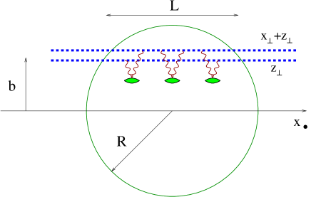
The nuclear matrix element of the two-Wilson-line operator (β€œcolor dipole”) is given by the Glauber formula, [22, 23, 24] see Fig. 2.

Refer to caption

FIG. 2.: Propagation of the color dipole through the nucleus.
$\displaystyle\int d^{2}z_{\perp}\langle A|{\rm Tr}U(x_{\perp}+z_{\perp})U(z_{\perp})|A\rangle$ (44)
$\displaystyle=~{}N_{c}\int d^{2}b\left[1-e^{-g^{2}c_{F}{\cal G}(x_{\perp}^{2})L_{b}}\right]$ (45)

Here $L_{b}\equiv 2\sqrt{R^{2}-b^{2}}$ is the propagation length of the dipole (located at the impact parameter $b$) through the nucleus, $\rho=\frac{A}{4/3\pi R^{3}}$ is the nuclear density, and

$${\cal G}(x_{\perp}^{2})\equiv\frac{\pi x_{\perp}^{2}}{4(N_{c}^{2}-1)}\rho\sigma_{0}G(\sigma_{0},\mu^{2}=\frac{1}{x_{\perp}^{2}}).$$ (46)

The Eq. (46) is derived under the assumption that the characteristic size of the dipole (the β€œsaturation scale ”) is smaller than the size of the nucleon ‑‑‑This assumption is certainly true at $A\rightarrow\infty$. For real nuclei, one should find the saturation scale $Q_{s}$ from the final result for the matrix element of the color dipole between the nuclear states, and verify that $Q_{s}\gg 1$GeV. In this case, the quarks propagating along the straight light-like lines §§§As we mentioned above, the energy $s\sigma_{0}$ should be high enough so we can replace the slope $p_{1}+\zeta_{0}p_{2}$ by $p_{1}$ in the non-logarithmical expressions. interact by the instantaneous (in the light-cone time $x_{+}$) potential

$\displaystyle\rho g^{2}t^{a}\otimes t^{a}\int\frac{d^{2}p_{\perp}}{(2\pi)^{2}}\frac{g^{2}}{2p_{\perp}^{4}}\Big{(}e^{i(p,x-y)_{\perp}}-1\Big{)}$ (47)
$\displaystyle=~{}g^{2}t^{a}\otimes t^{a}\rho\frac{\alpha_{s}}{8}(x-y)_{\perp}^{2}\ln(x-y)_{\perp}^{2}m_{0}^{2}$ (48)

where $m_{0}\simeq\frac{m_{N}}{2}$ is the IR cutoff.[23] It is worth noting that the factor $-1$ in the parenthesis in the l.h.s. comes from the diagrams with the two gluons attached to the same nucleon and the same Wilson line. Taking into account the color factors, one obtains the Eq. (45) with xB​G​(xB,ΞΌ2=xβŸ‚βˆ’2)=4​αsπ​ln⁑xβŸ‚βˆ’2/m02subscriptπ‘₯𝐡𝐺subscriptπ‘₯𝐡superscriptπœ‡2superscriptsubscriptπ‘₯perpendicular-to24subscriptπ›Όπ‘ πœ‹superscriptsubscriptπ‘₯perpendicular-to2superscriptsubscriptπ‘š02x_{B}G\big{(}x_{B},\mu^{2}=x_{\perp}^{-2}\big{)}=\frac{4\alpha_{s}}{\pi}\ln x_{\perp}^{-2}/m_{0}^{2}, see Ref. [23].

Similarly to Eq. (39), it is possible to represent this result as a functional integral over a variable $\Lambda(x_{\perp},l)\in SU(3)$:

∫d2​zβ€‹βŸ¨A|Ux+zΞ·0​Uz†η0|A⟩superscript𝑑2𝑧quantum-operator-product𝐴subscriptsuperscriptπ‘ˆsubscriptπœ‚0π‘₯𝑧subscriptsuperscriptπ‘ˆβ€ absentsubscriptπœ‚0𝑧𝐴\displaystyle\int d^{2}z\langle A|U^{\eta_{0}}_{x+z}U^{\dagger\eta_{0}}_{z}|A\rangle (49)
$\displaystyle=\int d^{2}b\int_{\Lambda(0,y)=1}^{\Lambda^{\prime}(L_{b},y)=0}D\Lambda(y,l)~{}\Lambda(x+z,L_{b})~{}\Lambda^{\dagger}(z,L_{b})$ (50)
$\displaystyle\hskip 28.45274pt\times~{}\exp\Big{\{}\frac{1}{2g^{2}\rho}\int_{0}^{L_{b}}\!dl\!\int\!d^{2}y\big{(}\Lambda(l,y)\Lambda^{\prime}(l,y)\big{)}^{a}$ (51)
$\displaystyle\hskip 56.9055pt\times~{}(-\vec{\partial}^{2}+m_{0}^{2})^{2}\big{(}\Lambda(l,y)\Lambda^{\prime}(l,y)\big{)}^{a}\Big{\}}$ (52)

where $\Lambda^{\prime}\equiv{\partial\over\partial l}\Lambda$. Extra $U^{\eta_{0}}(x)$ (U†η0​(x))superscriptπ‘ˆβ€ absentsubscriptπœ‚0π‘₯\big{(}U^{\dagger\eta_{0}}(x)\big{)} lead to extra $\Lambda(x,L_{b})$ $\big{(}\Lambda^{\dagger}(x,L_{b})\big{)}$ in the pre-exponent.

The final formula for the martix element of the color dipole operator at small $x_{B}$ is obtained by combining the functional integrals (39) and (49):

∫d2​zβ€‹βŸ¨A|UΞ·A​(x+z)βŠ—U†ηA​(z)|A⟩superscript𝑑2𝑧quantum-operator-product𝐴tensor-productsuperscriptπ‘ˆsubscriptπœ‚π΄π‘₯𝑧superscriptπ‘ˆβ€ absentsubscriptπœ‚π΄π‘§π΄\displaystyle\int d^{2}z\langle A|U^{\eta_{A}}(x+z)\otimes U^{\dagger\eta_{A}}(z)|A\rangle (53)
$\displaystyle=~{}\int\!d^{2}b\!\int_{\Lambda(0,y_{\perp})=1}^{\Lambda^{\prime}(L_{b},y_{\perp})=0}\int_{\Omega_{1,2}(\eta_{0},y)=1}^{\dot{\Omega}_{1,2}(\eta_{A},y)=0}D\Lambda(l,y)D\Omega_{1}(y,\eta)$ (54)
$\displaystyle\times~{}D\Omega_{2}(y,\eta)~{}\Omega^{\dagger}_{1}(x+z,\eta_{A})\Lambda(L_{b},x+z)$ (55)
$\displaystyle\otimes~{}\Omega_{2}(x+z,\eta_{A})\Omega^{\dagger}_{2}(z,\eta_{A})\Lambda^{\dagger}(L_{b},z)\Omega_{1}(z,\eta_{A})$ (56)
$\displaystyle\times~{}\exp\Bigg{\{}-\frac{1}{2g^{2}\rho}\int_{0}^{L_{b}}\!\!dl\int d^{2}y\big{(}i\Lambda(l,y)\Lambda^{\prime}(l,y)\big{)}^{a}$ (57)
$\displaystyle\hskip 71.13188pt\times~{}(m_{0}^{2}-\vec{\partial}^{2})^{2}\big{(}i\Lambda(l,y_{\perp})\Lambda^{\prime}(l,y)\big{)}^{a}$ (58)
βˆ’1Ξ±sβ€‹βˆ«Ξ·0Ξ·Aπ‘‘Ξ·β€‹βˆ«d2​yβ€‹βˆ‚β†’2​(i​Ω1†​(y,Ξ·)​Ω˙1​(y,Ξ·))a1subscript𝛼𝑠subscriptsuperscriptsubscriptπœ‚π΄subscriptπœ‚0differential-dπœ‚superscript𝑑2𝑦superscriptβ†’2superscript𝑖superscriptsubscriptΞ©1β€ π‘¦πœ‚subscriptΛ™Ξ©1π‘¦πœ‚π‘Ž\displaystyle-~{}\frac{1}{\alpha_{s}}\int^{\eta_{A}}_{\eta_{0}}d\eta\!\int\!d^{2}y\vec{\partial}^{2}\Big{(}i\Omega_{1}^{\dagger}(y,\eta)\dot{\Omega}_{1}(y,\eta)\Big{)}^{a} (59)
Γ—[βˆ‚β†’2​(Ξ©2†​(y,Ξ·)​Λ†​(Lb,y)​Ω1​(y,Ξ·))]a​bβˆ’1absentsubscriptsuperscriptdelimited-[]superscriptβ†’2superscriptsubscriptΞ©2β€ π‘¦πœ‚superscriptΛ†subscript𝐿𝑏𝑦subscriptΞ©1π‘¦πœ‚1π‘Žπ‘\displaystyle\hskip 42.67912pt\times~{}\Big{[}\vec{\partial}^{2}\Big{(}\Omega_{2}^{\dagger}(y,\eta)\Lambda^{\dagger}(L_{b},y)\Omega_{1}(y,\eta)\Big{)}\Big{]}^{-1}_{ab} (60)
$\displaystyle\hskip 71.13188pt\times~{}\vec{\partial}^{2}\Big{(}i\Omega_{2}^{\dagger}(y,\eta)\dot{\Omega}_{2}(y,\eta)\Big{)}^{b}\Bigg{\}}.$ (61)

The gluon structure function in the LLA is proportional to the matrix element of the dipole operator xB​G​(xB,ΞΌ2=xβŸ‚βˆ’2)=βˆ’2​πsβ€‹βŸ¨A|Tr​UiΞ·A​(xβŸ‚)​UiΞ·A​(0)|A⟩subscriptπ‘₯𝐡𝐺subscriptπ‘₯𝐡superscriptπœ‡2superscriptsubscriptπ‘₯perpendicular-to22πœ‹π‘ quantum-operator-product𝐴Trsuperscriptsubscriptπ‘ˆπ‘–subscriptπœ‚π΄subscriptπ‘₯perpendicular-tosuperscriptsubscriptπ‘ˆπ‘–subscriptπœ‚π΄0𝐴x_{B}G\big{(}x_{B},\mu^{2}=x_{\perp}^{-2}\big{)}=-\frac{2\pi}{s}\langle A|{\rm Tr}U_{i}^{\eta_{A}}(x_{\perp})U_{i}^{\eta_{A}}(0)|A\rangle, so the numerical calculation of the functional integral (61) should give the nuclear structure functions at small $x$. This would be complementary to the approximate solutions of Refs. [11, 17, 12, 19, 20, 26] since it could give the structure functions not only in the asymptotic black-body limit, but also in the intermediate region defining the saturation scale $Q_{s}$.

It should be mentioned that our formula (39) gives the evolution of the color dipole only in the LLA. In the case of large nucleus we have an additional parameter $A\gg 1$ so our LLA approximation based on the non-linear equation (4) has a window $\alpha_{s}^{2}A^{1/3}\sim 1$, $\alpha_{s}\ln x_{B}\sim 1$ where it is justified even at moderately small $x_{B}$. In the case of nucleon, our $\alpha_{s}(Q_{s})\ll 1$, $\alpha_{s}(Q_{s})\ln x_{B}\sim 1$ approximation should be justified a posteriori after checking that the saturation does occur at sufficiently small $x_{B}$. If the saturation takes place at such low $x$ that $\alpha_{s}(Q_{s})\ln x_{B}\gg 1$, our LLA breaks down and we need to take into account the non-fan diagrams such as t-channel loops formed by BFKL pomerons. However, the non-linear equation (4) leads to the result for the structure function which does not violate unitarity (see the discussion in Refs. [11, 12, 13, 17, 25]) and therefore we should not expect the large discrepancy between the unitary LLA result and the exact amplitude at present energies.


Acknowledgements.

The author is grateful to Y.V. Kovchegov, E.M. Levin and L. McLerran for valuable discussions. This work was supported by the US Department of Energy under contract DE-AC05-84ER40150.

REFERENCES

  • [1] V.S. Fadin, E.A. Kuraev, and L.N. Lipatov, Phys. Lett. B 60(1975), 50; I. Balitsky and L.N. Lipatov, Sov. Journ. Nucl. Phys. 28(1978), 822 .
  • [2] I. Balitsky, Nucl. Phys.B 463 (1996) 99.
  • [3] L.N. Lipatov, Phys. Reports 286 (1997) 131;
    I.Balitsky, β€œHigh-Energy QCD and Wilson Lines” , in the Boris Ioffe Festschrift β€œHandbook on QCD”, ed. M. Shifman (World Scientific, Singapore, 2001), e-print [hep-ph/0101042].
  • [4] O. Nachtmann, Annals Phys. 209, 436 (1991); J.C. Collins and R.K. Ellis, Nucl. Phys.B 360 (1991) 3.
  • [5] V.S. Fadin and L.N. Lipatov, Phys. Lett. B 429(1998) 127; G. Carnici and M. Ciafaloni, Phys. Lett. B 430(1998) 349 .
  • [6] Y.V. Kovchegov, A.H. Mueller, Phys. Lett. B 439(1998) 428 .
  • [7] L.V. Gribov, E.M. Levin, and M.G. Ryskin, Phys. Rept. 100(1983) 1 .
  • [8] A.H. Mueller and J.W. Qiu Nucl. Phys. B268(1986)427.
  • [9] L. McLerran and R. Venugopalan, Phys. Rev. D49 (1994) 2233; Phys. Rev. D49 (1994) 3352; Phys. Rev. D50 (1994) 2225.
  • [10] A.H. Mueller, Nucl. Phys. B558 (1999) 285.
  • [11] Yu.V. Kovchegov, Phys. Rev. D60, 034008 (1999); Phys. Rev. D61,074018 (2000).
  • [12] E. Levin and K. Tuchin, Nucl. Phys. BB573, 833 (2000).
  • [13] J. Jalilian-Marian, A. Kovner, L. McLerran, and H. Weigert, Nucl. Phys.B 504 (1997) 415; Phys. Rev. D59(1999) 014014; Phys. Rev. D59(1999) 034007;
  • [14] I. Balitsky, Phys. Rev. Lett. 81(1998) 2024, [hep-ph/9808215], Phys. Rev. D60, 014020 (1999).
  • [15] A.H. Mueller, Nucl. Phys. B415(1994) 373: A.H. Mueller and Bimal Patel, Nucl. Phys. B425(1994) 471.
  • [16] N.N. Nikolaev and B.G. Zakharov, Phys. Lett. B 332, 184 (1994); Z. Phys. C64, 631 (1994).
  • [17] M.A. Braun, Eur.Phys.J.C16(2000) 337.
  • [18] J. Bartels and M. Wusthoff, Z. Phys. C66, 157 (1995).
  • [19] E. Iancu and L. McLerran, Preprint SACLAY-T01-026 (hep-ph/0103032);
  • [20] H. Weigert, Preprint NORDITA-2000-34-HE (hep-ph/0004044);
  • [21] I. Balitsky and V.M. Braun, Nucl. Phys. B311, 541 (1989).
  • [22] B.Z Kopeliovich, I.L. Lapidus, and Al.B. Zamolodchikov, JETP Letters 33(1981) 612.
  • [23] A.H. Mueller, Nucl. Phys. B335 (1990) 115;
  • [24] Yu.V. Kovchegov and A.H. Mueller, Nucl. Phys. B529(1998) 451.
  • [25] A.H. Mueller, Nucl. Phys. B437 (1995) 107.
  • [26] E. Levin and K. Tuchin, Preprint TAUP-2659-2000 (hep-ph/0012167); Preprint TAUP-2664-2001 (hep-ph/0101275).