TUM-HEP-418/01 Reconstruction of the Earth’s matter density profile using a single neutrino baseline

Abstract

Abstract

In this paper, we show numerically that a symmetric Earth matter density profile can, in principle, be reconstructed from a single baseline energy spectrum up to a certain precision. For the numerical evaluations in the high dimensional parameter space we use a genetic algorithm.

Key words: neutrino oscillations, MSW effect, Earth’s matter density profile, neutrino tomography, genetic algorithm, geophysics
PACS: 14.60.Lm, 13.15.+g, 91.35.-x, 02.60.Pn

1 Introduction

In order to obtain knowledge about the Earth’s interior, current measurements are chiefly based on seismic wave propagation through the Earth (see, e.g., Refs. [1, 2]). The methods used in geophysics allow a quite precise reconstruction of the seismic wave velocity profile. However, for the determination of the matter density profile many assumptions have to be made about the equation of state, relating the velocity and matter density profiles. This process involves several uncertainties, since additional information about the Earth’s interior is quite rare (see, e.g., Refs.[3, 4]). In neutrino physics, a method similar to X-ray tomography has been suggested, namely neutrino absorption tomography [5, 6, 7, 8, 9, 10, 11, 12, 13]. It requires many different baselines, since neutrino absorption is not sensitive to the arrangement of the matter structure along one baseline. Moreover, the cross section rises with neutrino energy, which means that high energetic neutrinos are required.

Neutrino oscillations in the Earth have been extensively studied in general and it has been suggested that neutrino oscillations in matter can severely alter the energy spectrum of a neutrino beam through the Earth for long baselines [14, 15, 16, 17, 18, 19, 20, 21, 22, 23, 24, 25, 26, 27, 28, 29, 30]. For quite realistic calculations of the transition probabilities the Preliminary Reference Earth Model (PREM) or similar matter density profiles have been used [31, 32]. In addition, several approximations of the matter density profile, such as a step function (see, e.g., Refs. [33, 34]) or the first terms of a Fourier series expansion [35], turned out to supply rather good results. However, the inverse problem, i.e., what we can learn about the Earth’s structure from neutrino oscillations, is also considered to be an interesting problem. In Refs. [36, 37] the approach of an inverse scattering problem was suggested. However, transition probabilities of a single baseline energy spectrum turned out not to be sufficient for determining the matter density profile uniquely, i.e., additional information on the relative phase of the output state vector was required. In this paper, we ignore this information and investigate what we can learn about the Earth’s matter density profile from a single neutrino baseline energy spectrum using two flavor neutrino oscillations in matter. We show that we can, in principle, reconstruct the (symmetric) matter density profile, up to a certain precision without any additional assumptions about the profile itself. The (large-scale) symmetry of the matter density profile seems to be a reasonable assumption by the results from geophysics. Furthermore, since two flavor neutrino oscillations cannot distinguish time reverted matter density profiles (see, e.g., Refs. [38, 39]), omitting the symmetry condition would a priori mean that reconstructed, asymmetric profiles are not unique.

2 The model

For the numerical evaluation we use a (nondeterministic) genetic algorithm [40, 41]. It assumes an initial generation of random matter density profiles and calculates their respective energy spectra. The energy spectra are compared to a (realistic or measured) reference spectrum by an error (fitness) function. In this case, we choose minimization of a $\chi^{2}$-function [42]

$$\chi^{2}=\sum\limits_{i=1}^{B}2\left[\langle x_{i}\rangle-x_{i}\right]+2x_{i}\log\frac{x_{i}}{\langle x_{i}\rangle},$$ (1)

where $B$ is the number of energy bins, $x_{i}$ the (integer) number of events in the $i$th bin, and $\langle x_{i}\rangle$ the mean number of events in the $i$th bin. Nondeterministic evolution of the matter density profiles over time then creates an optimal or suboptimal matter density profile with an energy spectrum similar to the reference spectrum. Since the whole process is completely nondeterministic, the algorithm may find any symmetric matter density profile which fits the energy spectrum with the required precision. Thus, it also indicates if we are really able to obtain a unique solution for the given energy spectrum. The strength of applying a nondeterministic method is to reduce the exponential calculation effort to a polynomial one, where the quality of the obtained result can be determined by the statistical $\chi^{2}$-analysis. This means that we will find samples of the (high dimensional) parameter space within a (high dimensional) $n\sigma$-contour.

Here we use the neutrino appearance channel of a single neutrino baseline with an energy range from $2.5\,\mathrm{GeV}$ to $20\,\mathrm{GeV}$ (an energy range which may be produced by a neutrino factory), in order to cover the Mikheyev–Smirnov–Wolfenstein (MSW) resonance regions for reasonable data [43, 44, 45]. Since we are in principle interested in the reconstruction of the Earth’s matter density profile, we ignore information about the beam energy distribution and the cross sections, i.e., we use the transition probabilities directly. However, it is useful to have a statistical estimate of the significance of the results. Thus, we assume a total number of events $I$ to be folded with the transition probabilities equally spread over the whole energy spectrum at an equal cross section. Furthermore, we use a two flavor neutrino oscillation scenario with a symmetric PREM profile [31, 32]. For the propagation of a neutrino state vector along the baseline $L$ through the Earth, we divide the (symmetric) matter density profile into $2N$ layers of equidistant length $\Delta L\equiv\Delta L_{k}=L/(2N)$ of constant matter density $\rho_{k}$, where $k=1,2,\ldots,2N$, and we use an evolution operator in flavor basis in each individual layer $U_{f}(\Delta L_{k},\rho_{k})$ (see, e.g., Refs. [46, 47]). The total evolution operator $U_{f}(L)$ is then the time-ordered product of the ones in the individual layers, i.e., $U_{f}(L)=U_{f}(\Delta L_{2N},\rho_{2N})\ldots U_{f}(\Delta L_{2},\rho_{2})U_{f}(\Delta L_{1},\rho_{1})$. Finally, the transition probabilities are given by the absolute values squared of the elements of the total evolution operator, e.g., the transition probability for $\nu_{\alpha}\to\nu_{\beta}$ is $P_{\alpha\beta}(L)=|\langle\nu_{\beta}|U_{f}(L)|\nu_{\alpha}\rangle|$. Note that, because of the symmetry, $N$ is the number of independent parameters in this problem. The electron density $n_{e,k}$ is related to the matter density $\rho_{k}$ by

$$n_{e,k}=\frac{Y_{k}\rho_{k}}{m_{N}},\quad k=1,2,\ldots,2N,$$ (2)

where $Y_{k}$ is the average number of electrons per nucleon in the $k$th layer. In the Earth, $Y_{k}\simeq Y_{\rm Earth}\equiv 1/2$, $k=1,2,\ldots,2N$, and $m_{N}$ is the nucleon mass. For the baseline we choose $L=11736\,\rm{km}$, corresponding to a nadir angle of about $0.4$, in order to be able to see the Earth’s mantle as well as core in the energy spectra. Furthermore, for the oscillation parameters we use $\Delta m^{2}\equiv\Delta m_{32}^{2}=3.2\cdot\,10^{-3}\,\mathrm{eV}^{2}$ [48] and $\sin 2\theta\equiv\sin 2\theta_{13}=0.1$ [49, 50], which are applicable for a mass hierarchy $\Delta m_{21}^{2}\ll\Delta m_{32}^{2}$.

3 Results and analysis

We now present the results of some genetic algorithm trial runs. For the number of steps $N$ in the matter density profile we choose $N=4$, $N=9$, and $N=14$. We also compute the reference energy spectra with the PREM profile divided into $2N$ layers of constant matter density for $\chi^{2}\equiv\Delta\chi^{2}$ to be equal to zero at the minimum. In almost every example, we use a total number of events $I=100000$ to be folded with the transition probabilities, corresponding to a very optimistic guess of a very large neutrino factory, as well as a number of energy bins $B=31$. However, we will also investigate the precision for a varying number of events and energy bins.

The best fit results of the genetic algorithm are shown in Fig. 1

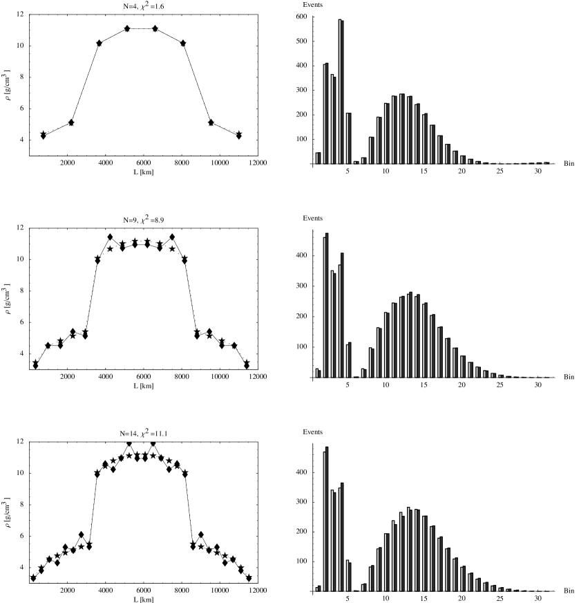
Figure 1: The best fits of the genetic algorithm trial runs for $N=4$, $N=9$, and $N=14$ steps in the Earth’s matter density profile. On the left-hand side the best fit matter density profiles (solid lines and boxes) are plotted with the reference profiles (dashed lines and stars). The values of $N$ and $\chi^{2}$ are given above each plot. On the right-hand side the energy bin spectra of the best fits (light bars) are shown together with the spectra of the reference (dark bars).

for several numbers of steps $N$ of the matter density profile. Note that the reference energy spectrum has two peaks corresponding to the mantle at high energy and the core as well as interference effects at low energy, respectively. All results in this figure are within a $1\sigma$ (68%) confidence region, which indicates that we cannot measure the matter density profile preciser without additional assumptions. Therefore, the precision of the measurement is limited for this type of experiment. Nevertheless, every trial run of the algorithm converges to a matter density profile clearly showing the mantle-core edge with high quality. It could not be seen in a Fourier expansion approach, since many Fourier coefficients had to be determined to obtain a high resolution of this edge [35].

The fact that the initial profiles were completely created at random, indicates that a single neutrino baseline energy spectrum really determines the arrangement and matter densities of the large-scale structure of the Earth’s matter density profile. Especially, in comparison to X-ray or neutrino tomography, it can distinguish the order of the different layers of matter because of the non-commuting operators used for the propagation through the matter density profile. The algorithm may have found any matter density profile matching the reference profile, such as one with mantle and core exchanged. Nevertheless, it turned out that it converged in all cases against the well-known mantle-core-mantle structure of the Earth. However, the non-commuting operators make the analytical inversion of the energy spectrum quite complicated (cf., Refs. [36, 37]).

As already mentioned above, the resolution of the matter density profile seems to be bounded. In order to investigate this, let us take a closer look at the parameter space. Since it is impossible to visualize the contours of equal confidence levels of a high dimensional problem, we plotted in Fig. 2 for $N=14$ some representatives of the parameter space

Figure 2: Representatives of the $N=14$-dimensional parameter space for $1\sigma$ (first row: $\chi^{2}\leq 15.9$), $2\sigma$ (second row: $\chi^{2}\leq 24.0$), and $3\sigma$ (third row: $\chi^{2}\leq 33.2$) confidence levels. The respective $\chi^{2}$’s of the samples are given above each plot. The sample matter density profiles are plotted with solid lines, whereas the reference profile is plotted with dashed lines.

within the $1\sigma$, $2\sigma$, and $3\sigma$ contours. Again, the mantle-core edge can be easily resolved at the $1\sigma$-level, but in many cases not for lower precision. It turns out that this effect grows with an increasing number of steps in the matter density profile. In addition, Figs. 1 and 2 indicate that the matter density profile can be quite well reconstructed for a small number of steps $N$, but for a higher number of steps $N$ small fluctuations enter the reconstructed profile. As can be seen in Fig. 2, we especially observe for $N=14$ small fluctuations in the mantle and core regions, indicating bounds on the spatial resolution. In App. A, we show analytically with a perturbation theoretical method what is intuitively clear: structures of small amplitude on a length scale $\lambda$ much smaller than the oscillation length in matter $L^{\mathrm{osc}}_{\mathrm{matter}}=4\pi E/\Delta\tilde{m}^{2}=4\pi E/[\xi(n_{e})\Delta m^{2}]$ cannot be resolved by neutrino oscillation in matter. Here

$$\xi(n_{e}) \equiv \sqrt{\left(\frac{2\sqrt{2}EG_{F}n_{e}}{\Delta m^{2}}-\cos 2\theta\right)^{2}+\sin^{2}2\theta}$$

is determined by the mean matter density $n_{e}$. Since $\xi\geq|\sin 2\theta|$, the upper bound $\lambda\simeq L^{\mathrm{osc}}_{\mathrm{matter}}<4\pi E/(\sin 2\theta\Delta m^{2})\propto E$ indicates that the higher the resonance energy of the resonance peak is, the lower the spatial resolution becomes. For this reason, the resolution of the core, corresponding to the low energy peak, is probably higher (cf., Figs. 1 and 2). However, for a realistic neutrino factory one has suppressions in low energetic events, which means that this effect is probably compensated by statistics [51].

In order to investigate the dependence on the total number of events $I$ and energy bins $B$, we show in Fig. 3 some matter density profile examples close to the $1\sigma$-contour for different numbers of $I$ and $B$.

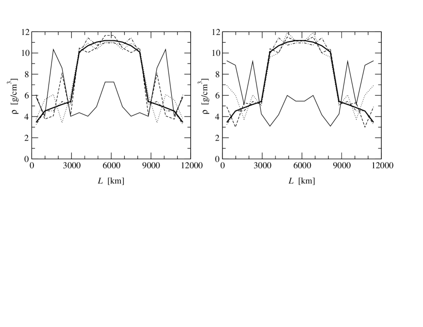
Figure 3: Matter density profiles for different numbers of total events $I$ (left) and different numbers of energy bins $B$ (right). The figures show matter density profiles close to the $1\sigma$-contour ($\chi^{2}\simeq 10.42$) for $N=9$ steps. The following matter density curves are plotted: In the left plot ($B=31$): Reference (thick solid); $I=1000$ (thin solid); $I=5000$ (dotted); $I=10000$ (dashed); $I=100000$ (dashed-dotted). In the right plot ($I=100000$): Reference (thick solid); $B=5$ (thin solid); $B=9$ (dotted); $B=16$ (dashed); $B=31$ (dashed-dotted).

One can see that the precision increases with the number of events. In almost all cases, we can clearly resolve the mantle-core edge, but for too few events $I\ll 5000$ the result does not have a physical meaning anymore. One can also see that the precision increases with the number of energy bins $B$. In addition, for $B=5$ the matter density profile again looses its physical meaning. Note that, since we did not integrate over the energy of each bin, but used the mean energy, there is a statistical error increasing with decreasing number of energy bins. However, one may expect a natural boundary of the evaluation for $B<N$, because $N$ represents the number of unknowns and $B$ the number of equations. This equivalence between the number of equations and the number of energy bins would be destroyed for an integration over the energy within each energy bin.

4 Summary and conclusions

In summary, we have demonstrated that we can, in principle, reconstruct the symmetric Earth matter density profile using a single neutrino baseline energy spectrum without additional assumptions. However, it turned out that the precision is limited in this method, especially since we made quite optimistic assumptions about the total number of detectable events $I$ and the energy spectrum of the source, as well as we ignored any energy smearing.

We conclude that neutrino physics cannot be used as the only source for obtaining information about the Earth’s interior, since the precision is presently lower than in geophysics, and the resolution has a natural lower bound, the oscillation length in matter. However, geophysics can only access the velocity profile of seismic waves directly. Additional assumptions about the equation of state have to be made in order to access the matter density profile. Thus, neutrino oscillations in matter could help to test and verify the equation of state. Similarly, the parameter space in neutrino reconstruction tomography could be shrinked by using knowledge from geophysics.

Appendix A Spatial resolution of neutrino oscillations in matter

In this appendix, we will show in the case of two neutrino flavors that we cannot resolve structures much smaller than the oscillation length in matter. For that we state the differential equation describing the time evolution of flavor states in matter:

$$i\frac{d}{dt}\nu_{f}(t)=\mathcal{H}_{0}\,\nu_{f}(t)+\mathcal{H}_{\mathrm{int}}(n_{e})\,\nu_{f}(t)$$ (4)

with $\nu_{f}(t)=(\nu_{e}(t),\nu_{\mu}(t))^{T}$,

$$\mathcal{H}_{0}=\left(\begin{array}[]{cc}-\frac{\Delta m^{2}}{4E}\cos 2\theta&\frac{\Delta m^{2}}{4E}\sin 2\theta\\ \frac{\Delta m^{2}}{4E}\sin 2\theta&\frac{\Delta m^{2}}{4E}\cos 2\theta\\ \end{array}\right),$$ (5)

and

$$\mathcal{H}_{\mathrm{int}}(n_{e})=\left(\begin{array}[]{cc}\sqrt{2}G_{F}n_{e}&0\\ 0&0\end{array}\right).$$ (6)

Let us introduce a perturbation $\eta(t)$ on a shorter timescale than a slowly varying matter density profile $\tilde{n}_{e}(t)$, i.e.,

$$n_{e}(t)=\tilde{n}_{e}(t)+\eta(t)$$ (7)

with $\eta(t)$ making many oscillations while $\tilde{n}_{e}(t)$ is approximately constant. This will also result in a modification of the amplitudes

$$\nu_{f}(t)=\tilde{\nu}_{f}(t)+\chi_{f}(t),$$ (8)

where $\tilde{\nu}_{f}(t)$ solves the unperturbed equations for $\mathcal{H}_{\mathrm{int}}(\tilde{n}_{e})$. Thus, we can split Eq. (4) by applying Eqs. (7) and (8) and we obtain

$$i\frac{d}{dt}\tilde{\nu}_{f}(t) = \mathcal{H}_{0}\,\tilde{\nu}_{f}(t)+\mathcal{H}_{\mathrm{int}}(\tilde{n}_{e}(t))\,\tilde{\nu}_{f}(t),$$

$$i\frac{d}{dt}\chi_{f}(t) = \mathcal{H}_{0}\,\chi_{f}(t)+\mathcal{H}_{\mathrm{int}}(\tilde{n}_{e}(t))\,\chi_{f}(t)$$ (10)

$$+ \mathcal{H}_{\mathrm{int}}(\eta(t))\,\tilde{\nu}_{f}(t).$$

Here we have neglected second order corrections of the order $\eta(t)\chi(t)$. We know that the oscillation of the solution of the first equation is determined by the oscillation length in matter $L^{\mathrm{osc}}_{\mathrm{matter}}=4\pi E/\Delta\tilde{m}^{2}=4\pi E/[\xi(\tilde{n}_{e})\Delta m^{2}]$, where the $\xi$ was defined in Eq. (LABEL:xi) and refers here to the constant mean matter density $\tilde{n}_{e}$.. For the second equation, we may assume a quick periodic oscillation $\eta(t)=A\cos(\omega t)$ with the amplitude $A$ and the frequency $\omega$ on a timescale much shorter than the one of the first equation. Hence, we can in the second equation take $\tilde{\nu}_{f}(t)\simeq\tilde{\nu}_{f}$ and $\tilde{n}_{e}(t)\simeq\tilde{n}$ approximately to be constant.

We can thus rewrite Eq. (10) as

$$i\frac{d}{dt}\chi_{f}(t) = \mathcal{H}_{0}\,\chi_{f}(t)+\mathcal{H}_{\mathrm{int}}(\tilde{n}_{e})\,\chi_{f}(t)$$ (11)

$$+ \mathcal{H}_{\mathrm{int}}(\tilde{\nu}_{e})\,A\cos(\omega t).$$

This is a differential system of equations similar to the one for two coupled oscillators, where the one representing the electron flavor is driven by an external force corresponding to the oscillatory fluctuation in the matter density profile. It is solved by quite lengthy, purely oscillatory expressions for $\chi_{e}(t)$ and $\chi_{\mu}(t)$.

One can show that the amplitudes of the oscillations reduce to zero when $\omega\gg\xi(\tilde{n}_{e})\,\Delta m^{2}/(2E)\equiv 2\pi/L^{\mathrm{osc}}_{\mathrm{matter}}$. Since $\omega=2\pi/\lambda$, this means that we cannot resolve structures in the matter density profile with a width $\lambda\ll L^{\mathrm{osc}}_{\mathrm{matter}}$. Note that the perturbation method used breaks down for too large amplitudes or too slow oscillations.

References

- [1] K. Aki and P.G. Richards, Quantitative Seismology: Theory and Methods (W. H. Freeman, 1980), Vol. 1, 2.
- [2] T. Lay and T.C. Wallace, Modern Global Seismology (Academic Press, 1995).
- [3] R. Jeanlow and S. Morris, Ann. Rev. Earth Plan. Sci. 14 (1986) 377.
- [4] R. Jeanlow, Ann. Rev. Earth Plan. Sci. 18 (1990) 357.
- [5] L.V. Volkova and G.T. Zatsepin, Bull. Phys. Ser. 38 (1974) 151.
- [6] A. De Rújula et al., Phys. Rep. 99 (1983) 341.
- [7] T.L. Wilson, Nature 309 (1984) 38.
- [8] G.A. Askar’yan, Usp. Fiz. Nauk 144 (1984) 523, [Sov. Phys. Usp. 27 (1984) 896].
- [9] A. Borisov, B. Dolgoshein and A. Kalinovskii, Yad. Fiz. 44 (1986) 681, [Sov. J. Nucl. Phys. 44 (1987) 442].
- [10] A. Nicolaidis, M. Jannane and A. Tarantola, J. Geophys. Res. 96 (1991) 21811.
- [11] H.J. Crawford et al., Proc. of the XXIV International Cosmic Ray Conference (University of Rome) (1995) 804.
- [12] C. Kuo et al., Earth Plan. Sci. Lett. 133 (1995) 95.
- [13] P. Jain, J.P. Ralston and G.M. Frichter, Astropart. Phys. 12 (1999) 193, hep-ph/9902206.
- [14] V.K. Ermilova, V.A. Tsarev and V.A. Chechin, Pis’ma Zh. Eksp. Teor. Fiz. 43 (1986) 353, [JETP Lett. 43 (1986) 453].
- [15] A.J. Baltz and J. Weneser, Phys. Rev. D35 (1987) 528.
- [16] A. Nicolaidis, Phys. Lett. B200 (1988) 553.
- [17] P.I. Krastev and S.T. Petcov, Phys. Lett. B205 (1988) 84.
- [18] T.K. Kuo and J. Pantaleone, Rev. Mod. Phys. 61 (1989) 937.
- [19] P.I. Krastev and A.Y. Smirnov, Phys. Lett. B226 (1989) 341.
- [20] Y. Minorikawa and K. Mitsui, Europhys. Lett. 11 (1990) 607.
- [21] S.T. Petcov, Phys. Lett. B434 (1998) 321, hep-ph/9805262.
- [22] E.K. Akhmedov, Nucl. Phys. B538 (1999) 25, hep-ph/9805272.
- [23] E.K. Akhmedov et al., Nucl. Phys. B542 (1999) 3, hep-ph/9808270.
- [24] M.V. Chizhov and S.T. Petcov, Phys. Rev. Lett. 83 (1999) 1096, hep-ph/9903399.
- [25] M.V. Chizhov and S.T. Petcov, Phys. Rev. D63 (2001) 073003, hep-ph/9903424.
- [26] E.K. Akhmedov, Pramana 54 (2000) 47, hep-ph/9907435.
- [27] I. Mocioiu and R. Shrock, Phys. Rev. D62 (2000) 053017, hep-ph/0002149.
- [28] M. Freund, P. Huber and M. Lindner, Nucl. Phys. B585 (2000) 105, hep-ph/0004085.
- [29] K. Dick et al., Nucl. Phys. B598 (2001) 543, hep-ph/0008016.
- [30] E.K. Akhmedov, hep-ph/0008134.
- [31] F.D. Stacey, Physics of the Earth, 2 ed. (Wiley, 1977).
- [32] A.M. Dziewonski and D.L. Anderson, Phys. Earth Planet. Inter. 25 (1981) 297.
- [33] M. Freund and T. Ohlsson, Mod. Phys. Lett. A15 (2000) 867, hep-ph/9909501.
- [34] M. Freund et al., Nucl. Phys. B578 (2000) 27, hep-ph/9912457.
- [35] T. Ota and J. Sato, hep-ph/0011234.
- [36] V.K. Ermilova, V.A. Tsarev and V.A. Chechin, Bull. Lebedev Phys. Inst. NO.3 (1988) 51.
- [37] V.A. Chechin and V.K. Ermilova, Proc. of LEWI’90 School, Dubna (1991) 75.
- [38] A. de Gouvêa, Phys. Rev. D63 (2001) 093003, hep-ph/0006157.
- [39] E.K. Akhmedov, Phys. Lett. B503 (2001) 133, hep-ph/0011136.
- [40] D.E. Goldberg, Genetic Algorithms in Search, Optimization, and Machine Learning (Addison-Wesley, 1989).
- [41] J.A. Freeman, Simulating Neural Networks with Mathematica (Addison-Wesley, 1994).
- [42] Particle Data Group, D.E. Groom et al., Eur. Phys. J. C15 (2000) 1, http://pdg.lbl.gov/.
- [43] S.P. Mikheyev and A.Y. Smirnov, Yad. Fiz. 42 (1985) 1441, [Sov. J. Nucl. Phys. 42 (1985) 913].
- [44] S.P. Mikheyev and A.Y. Smirnov, Nuovo Cimento C 9 (1986) 17.
- [45] L. Wolfenstein, Phys. Rev. D 17 (1978) 2369.
- [46] T. Ohlsson and H. Snellman, Phys. Lett. B474 (2000) 153, hep-ph/9912295, B480 (2000) 419(E).
- [47] T. Ohlsson and H. Snellman, Eur. Phys. J. C (to be published), hep-ph/0103252.
- [48] Super-Kamiokande, S. Fukuda et al., Phys. Rev. Lett. 85 (2000) 3999, hep-ex/0009001.
- [49] CHOOZ, M. Apollonio et al., Phys. Lett. B420 (1998) 397, hep-ex/9711002.
- [50] CHOOZ, M. Apollonio et al., Phys. Lett. B466 (1999) 415, hep-ex/9907037.
- [51] V. Barger, S. Geer and K. Whisnant, Phys. Rev. D61 (2000) 053004, hep-ph/9906487.