Status of the Gribov–Pontecorvo Solution to the Solar Neutrino Problem

Abstract

We discuss the status of the Gribov–Pontecorvo (GP) solution to the solar neutrino problem. This solution naturally appears in bimaximal neutrino mixing and reduces the solar and atmospheric neutrino problems to vacuum oscillations of three active neutrinos. The GP solution predicts an energy-independent suppression of the solar neutrino flux. It is disfavoured by the rate of the Homestake detector, but its statistical significance greatly improves, when the chlorine rate and the boron neutrino flux are slightly rescaled, and when the Super-Kamiokande neutrino spectrum is included in the analysis. Our results show that rescaling of the chlorine signal by only $10\%$ is sufficient for the GP solution to exist, if the boron–neutrino flux is taken $10$ – $20\%$ lower than the SSM prediction. The regions allowed for the GP solution in the parameter space are found and observational signatures of this solution are discussed.

I Introduction

Vacuum oscillations of maximally mixed $\nu_{\mu}$ and $\nu_{\tau}$ neutrinos with $(\Delta m^{2})_{\rm atm}\sim 3\times 10^{-3}$ eV² are the favourite explanation of the atmospheric neutrino anomaly. A natural generalization is bimaximal mixing [1]–[10] of three active neutrinos, when mixing is described by the following matrix:

$$\left(\begin{array}[]{c}\nu_{e}\\ \nu_{\mu}\\ \nu_{\tau}\end{array}\right)=\left(\begin{array}[]{ccc}\frac{1}{\sqrt{2}}&-\frac{1}{\sqrt{2}}&0\\ \frac{1}{2}&\frac{1}{2}&\frac{1}{\sqrt{2}}\\ \frac{1}{2}&\frac{1}{2}&-\frac{1}{\sqrt{2}}\end{array}\right)\left(\begin{array}[]{c}\nu_{1}\\ \nu_{2}\\ \nu_{3}\end{array}\right)\;.$$ (1)

In the case of the mixing matrix given by Eq. (1), the solar neutrino oscillation is also maximal. To see this, it should be noted from Eq. (1) that

$$\frac{1}{\sqrt{2}}(\nu_{\mu}-\nu_{\tau})=\nu_{3},$$ (2)

while the other orthogonal combination of these states can be considered as a new field

$$\nu^{\prime}=\frac{1}{\sqrt{2}}(\nu_{\mu}+\nu_{\tau})\;.$$ (3)

Using the above equations, one obtains

$$\left(\begin{array}[]{c}\nu_{e}\\ \nu^{\prime}\\ \nu_{\tau}\end{array}\right)=\left(\begin{array}[]{ccc}\frac{1}{\sqrt{2}}&-\frac{1}{\sqrt{2}}&0\\ \frac{1}{\sqrt{2}}&\frac{1}{\sqrt{2}}&0\\ \frac{1}{2}&\frac{1}{2}&\frac{1}{\sqrt{2}}\end{array}\right)\left(\begin{array}[]{c}\nu_{1}\\ \nu_{2}\\ \nu_{3}\end{array}\right)\;.$$ (4)

From Eq. (4) it follows that $\nu_{e}$ and $\nu^{\prime}=1/\sqrt{2}(\nu_{\mu}+\nu_{\tau})$ are a maximally mixed pair, and the flavour eigenstate $\nu_{e}$ is oscillating on the way from the Sun into $\nu^{\prime}$, the coherent mixture of $\nu_{\mu}$ and $\nu_{\tau}$.

The above exercise is relevant to the Gribov–Pontecorvo (GP) [11] solution of the solar neutrino problem combined with atmospheric $\nu_{\mu}$–$\nu_{\tau}$ oscillations. Following [11], the definition of the GP solution can be given by two conditions: (i) smallness of the oscillation length $l_{\nu}$ with respect to the mean distance between the Sun and the Earth $\langle r\rangle=L$

$$l_{\nu}=\frac{4\pi E}{\Delta m^{2}}\ll L=1.5\times 10^{13}~{}{\rm cm},$$ (5)

and (ii) smallness of the matter corrections (MSW [19]) in the Sun and in the Earth [20] (in Ref.[11] only vacuum oscillation is considered).

Indeed, in this case the averaged survival probability for $\nu_{e}$ is

$$\langle P_{ee}\rangle=1-\sin^{2}2\theta\langle\sin^{2}\frac{\Delta m^{2}r}{4E}\rangle=1-\frac{1}{2}\sin^{2}2\theta\equiv P_{\rm GP},$$ (6)

and from comparison with experimental data, $P_{ee}\sim 0.5$, we come to $\theta\sim\pi/4$, or to bimaximal mixing if $\nu_{\mu}\leftrightarrow\nu_{\tau}$ explains atmospheric neutrino oscillations.

Three remarks are immediately in order.

(i) There is no theoretical reason for bimaximal mixing to be exact, and more generally one should consider near-bimaximal mixing [1, 18].

(ii) The smallness of the matter correction effects, which we included in the definition of the GP solution is actually not needed in the case of near-bimaximal mixing if only matter effects in the Sun are included. For the exact maximal mixing, $\nu_{e}\to\nu^{\prime}$ conversion in the Sun does not change the total survival probability $\langle P_{ee}\rangle$ at the surface of the Earth [15, 9]. In the arbitrary case where the mixing between $\nu_{e}$ and $\nu^{\prime}$ is described by the mixing angle $\theta$, and the MSW effect in the Sun converts $\nu_{e}$ into $\nu_{S}=\cos\theta_{S}\nu_{1}+\sin\theta_{S}\nu_{2}$ (subscript $S$ here refers to the surface of the Sun), the total survival probability $\langle P_{ee}\rangle=|\langle\nu_{E}|\nu_{e}\rangle|^{2}$ on the surface of the Earth can be readily calculated as

$$\langle P_{ee}\rangle=\cos^{2}\theta_{S}\cos^{2}\theta+\sin^{2}\theta_{S}\sin^{2}\theta$$ (7)

For exact bimaximal mixing $\cos^{2}\theta=\sin^{2}\theta=1/2$, survival probability $\langle P_{ee}\rangle=1/2$ and thus it does not depend on $\theta_{S}$, i.e. on how $\nu_{e}$ is converted in the Sun. For near-bimaximal mixing, Eq. (7) determines a narrow range of $\theta$ near $\pi/4$, where $\langle P_{ee}\rangle$ is practically energy independent, i.e. it does not depend on $\theta_{S}$. The matter effect in the Earth, however, changes this conclusion as we shall see in the next section.

(iii) The observational data (see Fig. 1) do not support $\langle P_{ee}\rangle$ being exactly energy-independent. While the recent Super-Kamiokande (SK) data agree well with $\langle P_{ee}\rangle$ being an energy-independent constant in the energy interval 5 – 14 MeV, the values $\langle P_{ee}\rangle$ from three different experiments, GALLEX–GNO/SAGE, Homestake and Kamiokande/SK, are not exactly the same.

The aim of this paper is to discuss quantitatively the status of the GP solution. An interesting region in the parameter space is given by $\Delta m^{2}\lesssim 10^{-3}~{}{\rm eV}^{2}$ and $\theta\sim\pi/4$, where bimaximal mixing is characterized by $(\Delta m^{2})_{\rm atm}$ and $(\Delta m^{2})_{\rm sol}$ not very different from each other, and where the MSW effect is allowed as a small correction.

Oscillations with energy-independent suppression were suggested and studied in many works before [12, 13, 14, 15, 16] and most notably in the recent work of Ref. [17]. In all these works the authors have realized that the observed rate in the chlorine experiment (Homestake [25]) contradicts the energy-independent suppression, and it has to be taken larger than the observed one for it to work. In this paper we argue that $10\%$ excess could be sufficient. Note, that the solution with energy-independent suppression is more general than the GP solution, because in the latter $l_{\nu}\ll L$ is assumed, while the energy-(quasi)independent solution might appear in some other regions of the parameter space.

II Parameter space regions for the GP solution

In this section we shall calculate the regions allowed for the GP solution in the parameter space $\Delta m^{2}$, $\tan^{2}\theta$. We first define the oscillation parameter space where the solar neutrino survival probability behaves effectively as the GP one. In order to do so we impose the condition that for any of the $i$ solar neutrino fluxes (integrated over the different production point distributions) the survival probability in the relevant range of energies does not differ by more than 10% (1%) from $P_{\rm GP}$ given by Eq. (6):

$$\frac{|P_{ee}^{i}(E/\Delta m^{2},\theta)-P_{\rm GP}(\theta)|}{P_{\rm GP}(\theta)}<0.1\;(0.01)\;\;\;\;\mbox{\rm for}\;\;E_{i,max}>E>E_{i,min},$$ (8)

where $E_{i,max}$ and $E_{i,min}$ determine the range of energies in which the flux $i$ is detected in present experiments. For instance, for $i=pp$, $E_{pp,min}=0.233$ MeV and $E_{pp,max}=0.42$ MeV. In the evaluation of the corresponding survival probabilities, we have included the matter effects when propagating in the Sun and in the Earth as well as the distance interference term:

$$P_{ee}^{i}=P^{S}_{e,1}P^{E}_{1,e}+P^{S}_{e,2}P^{E}_{2,e}+2\sqrt{P^{S}_{e,1}P^{S}_{e,2}P^{E}_{1,e}P^{E}_{2,e}}\cos\frac{\Delta m^{2}_{21}(L)}{2E}\;,$$ (9)

where $P^{S}_{e,i}$ is the probability for the $\nu_{e}$ to exit the Sun in the mass eigenstate $i$, while $P^{E}_{i,e}$ is the probability for the mass eigenstate $i$ arriving at the Earth to reach the detector as a $\nu_{e}$. $L$ is the average distance between the Sun and the Earth.

In Fig. 2 we show the parameter space $\Delta m^{2}$, $\tan^{2}\theta$ where the condition given by Eq. (8) is verified at 10% (lighter shadow) and 1% (darker shadow). The only interesting sector of the effective–GP region in this parameter space is located at large $\Delta m^{2}$ around the maximal mixing line $\tan^{2}\theta=1$, where matter effects in the Sun are suppressed. This region is limited from above by the CHOOZ reactor data [27]. Only in this sector there is an overlap with the rate- and spectra-allowed regions (see below).

As was discussed above, for maximal mixing the matter effects in the Sun do not alter the energy-independent survival probability $P_{ee}$ on the way from the production point inside the Sun to the surface of the Earth. However Earth matter effects make $P_{ee}$ energy-dependent in the regions of maximal mixing at $10^{-5}\lesssim\Delta m^{2}\lesssim 10^{-8}$. In contrast with our calculations, the region $\Delta m^{2}\lesssim 10^{-7}$ is found in ref.[17] as energy-independent one. We explain this discrepancy by two effects:

• For $10^{-8}\lesssim\Delta m^{2}\lesssim 10^{-7}$ Earth matter effects for $pp$-neutrinos result into an energy dependence of the survival probability beyond 10%.

• At $\Delta m^{2}\lesssim 10^{-8}$ the $L$ dependent interference term in Eq. (9) gives strong energy dependence of the ⁸B flux. This term was not included in the calculations of Ref.[17].

As we mentioned above, the GP solution is incompatible with the central value of the rate measured by the Homestake detector $R_{\rm Cl}=2.56$ SNU [25]. Following the prescription of many works, we shall use the rescaled rate $R_{\rm Cl}^{\rm res}=2.56f_{\rm Cl}$ SNU, assuming $f_{\rm Cl}\gtrsim 1$ to be a free parameter. In Fig. 3 we plot the $\chi^{2}$ function from the analysis of the three observed rates as a function of the $f_{\rm Cl}$ factor for different constant values of the survival probability $P_{\rm GP}=0.5,0.59$ and 0.71. The upper left panel corresponds to oscillations into active neutrinos while the lower one into sterile neutrinos. The differences between these two scenarios arise from the absence of NC contribution to the SK rate in case of oscillations into sterile neutrinos. From this figure we see that the best GP-like solution corresponds to survival probability slightly larger than that for maximal–mixing case (close to 0.59) both for active and sterile neutrinos. The quality of these solutions are considerably improved when allowing a 30–50 % increase in $f_{\rm Cl}$. This improvement is more significant for the case of sterile neutrinos since the corresponding survival probability at SK agrees better with the data from gallium detectors (see Fig.1).

This behaviour is also illustrated in Fig. 4 where we show the $\Delta m^{2}$, $\tan^{2}\theta$ regions allowed by the statistical analysis of the rates of GALLEX–GNO/SAGE [22, 23, 21], SK [24] and Chlorine[25] experiments for different values of $f_{\rm Cl}$ in case of active and sterile neutrinos, and for Bahcall-Pinsonneault (BP00) [26] fluxes. The solutions, following the standard statistical analysis (for details see Ref. [28]), are shown at 99% CL. The effective GP solutions are marked as dark areas. Notice that they appear at $f_{\rm Cl}\gtrsim 1.1$ (1.2) for active (sterile) oscillations and that all regions displayed have a cut at $\Delta m^{2}\approx 8\times 10^{-4}$ as a consequence of the CHOOZ [27] bound.

Inclusion of SK data on the energy spectra of boron neutrinos improves the quality of the GP solution. In Fig. 5 we display, for different values of $f_{\rm Cl}$, the regions allowed by the analysis of the rates and day–night spectrum of boron neutrinos measured by SK [24]. Again the solutions are shown at 99% CL and the effective GP solutions are marked as dark areas. From these figures one can see that the inclusion of the spectra data results in the appearance of allowed regions for the GP solutions at smaller values of $f_{\rm Cl}$. This is a natural result, because the rates of GALLEX–GNO/SAGE and Homestake can be also considered as information about the solar neutrino spectrum, in its low energy part, however in contrast to the low energy part of the spectrum, the GP solution describes well the spectrum observed in SK.

In Figs. 4–5 we have used the boron neutrino flux as calculated in the Standard Solar Model [26]. This flux has a large theoretical uncertainty mostly due to uncertainties in the pBe cross-section. In order to study the effect of a possible deviation of the ⁸B flux from the SSM prediction [26], we shall introduce the rescaled boron neutrino flux defined as $\Phi_{\rm B}=f_{\rm B}\Phi_{\rm B}^{\rm SSM}$ with $\Phi_{\rm B}^{\rm SSM}$ given by [26]. In the central panels in Fig. 3, we plot the $\chi^{2}$ function from the analysis of the three observed rates as a function of $f_{\rm Cl}$ for different constant values of the survival probability $P_{\rm GP}$ when the factor $f_{\rm B}$ is left free. The upper central panel corresponds to oscillations into active neutrinos, the lower one into sterile neutrinos. In the right panels we show the corresponding values of $f_{\rm B}$, which give the best agreement with the data for each value of $f_{\rm Cl}$ and $P_{\rm GP}$. From this figure we find that although using a free $f_{\rm B}<1$ leads to a further increase of the statistical significance of the GP solution, it has a smaller impact than the corresponding variation of $f_{\rm Cl}$. It, however, allows for the presence of GP solutions with smaller $f_{\rm Cl}$. This is particularly the case for oscillations into active neutrinos.

In Fig. 6 we plot the allowed regions from the analysis of the rates and day–night spectrum of ⁸B neutrinos measured by SK for different values of $f_{\rm Cl}$ and $f_{\rm B}$. For the sake of concreteness we have chosen the $f_{\rm B}$ factor that gives a better fit to the three rates for each value of $f_{\rm Cl}$ for maximal mixing. Namely, $f_{\rm B}$ is chosen as $f_{\rm B}\sim 0.8$ (0.9) for oscillations into active (sterile) neutrinos. In Fig. 6 the left panels correspond to oscillations into active neutrinos and the right ones into sterile neutrinos. Comparing this figure with the corresponding panels in Figs. 5 we see that lowering the ⁸B normalization leads to a larger overlap between the allowed LMA region and the GP solution already for $f_{\rm Cl}\leq 1.1$, in the case of oscillations into active neutrinos.

III Conclusions

It could be that nature has chosen the most unsophisticated scheme of neutrino oscillations: three active neutrinos with (nearly) bimaximal mixing. Mixing of $\nu_{\mu}$ and $\nu_{\tau}$ explains the atmospheric neutrino anomaly, and of $\nu_{e}$ and $\nu^{\prime}=(1/\sqrt{2})(\nu_{\mu}+\nu_{\tau})$ the solar neutrino deficit. In this case, the GP solution, provided by condition (5), naturally appears, and it is characterized by an energy-independent survival probability $\langle P_{ee}\rangle=P_{\rm GP}$.

The GP solution is disfavoured by the Homestake rate, but describes well the other rates as well as the energy spectrum observed in SK. The statistical significance of the GP solution strongly improves if one assumes rescaling of the chlorine rate by a factor $f_{\rm Cl}=1.1$–$1.5$, while some further improvement arises if the ⁸B neutrino flux is also rescaled by a factor $f_{\rm B}=0.7$–$0.9$. In particular if the ⁸B flux happens to be 10–20% lower than the BP00-predicted central value, the GP solution for maximal mixing in active oscillations would be a llowed with a chlorine rescaling factor $f_{\rm Cl}\lesssim 1.1$.

The GP solution will be directly searched for in the KamLand experiment [29]. Detection of reactor neutrinos can result in the measurement of $\Delta m^{2}$ in the interval $10^{-3}$–$3\times 10^{-6}~{}{\rm eV}^{2}$ for large mixing angles. If $\Delta m^{2}$ is found outside the LMA MSW region or inside it at $\theta\approx\pi/4$, would mean the discovery of the GP solution.

In low energy solar neutrino experiments the signatures of the GP solution are the ordinary suppression of ⁷Be neutrinos given by a factor $P_{\rm GP}=\frac{1}{2}\sin^{2}2\theta$ and the absence of anomalous seasonal variations (beyond the geometrical ones). These features can be clearly seen in Borexino [30] and KamLand [29] experiments.
Note
This work was presented by M.C.Gonzalez-Garcia at the Gran Sasso Laboratory at the 5th Topical Workshop on “Solar Neutrinos: Where are the Oscillations?” (March 2001). On March 29 the preprint by S. Choubey, S. Coswami, N. Gupta and D.P. Roy [17] appeared in the net. The basic assumptions they used, rescaling of the chlorine and boron fluxes, are the same as in our paper, but we are considering a GP solution that is not, in principle, identical to the energy-independent solution, studied in the aforementioned paper. The most noticeable difference in our results relates to the low $\Delta m^{2}$ solutions found in Ref.[17] and shown in their figures 1 -4. They are not present in our solutions partly due to interference term given in our Eq.(9) and disregarded in Ref.[17].

FIG. 1.: Ratios of observed rates to the BP00 prediction for the existing experiments. In the case of oscillations the ratios for all experiments, except Super-Kamiokande, are equal to the $\nu_{e}$ survival probability $P_{ee}$. For Super-Kamiokande the ratio SK gives $P_{ee}$ in the case of oscillation to sterile neutrinos, while for the case of oscillation to active neutrino we plot the corresponding $P_{ee,ac}$.

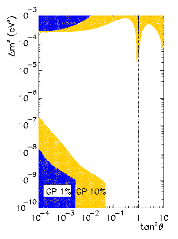
FIG. 2.: Regions in $\Delta m^{2}$, $\tan^{2}\theta$ parameter space, where the $\nu_{e}$ survival probability $P_{ee}(E)$ differs from the energy-independent GP survival probability $P_{\rm GP}$ by less than 10% (lighter shadow) and less than 1% (dark shadow). See the text for details.

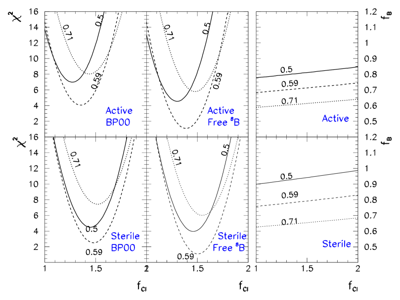
FIG. 3.: $\chi^{2}$ analysis of the three observed rates as a function of the $f_{\rm Cl}$ factor for different constant values of the survival probability $P_{\rm GP}=0.5,0.59$ and $0.71$ (solid, dashed and dotted lines respectively). The upper (lower) panels correspond to oscillations into active (sterile) neutrinos. In the left panels we have used BP00 boron fluxes ($f_{\rm B}=1$), while in the central panels $f_{\rm B}$ is left free to optimize $\chi^{2}$. The resulting $f_{\rm B}$ values which optimize $\chi^{2}$ for given $f_{\rm Cl}$ and $P_{\rm GP}$ are plotted in the right panels.

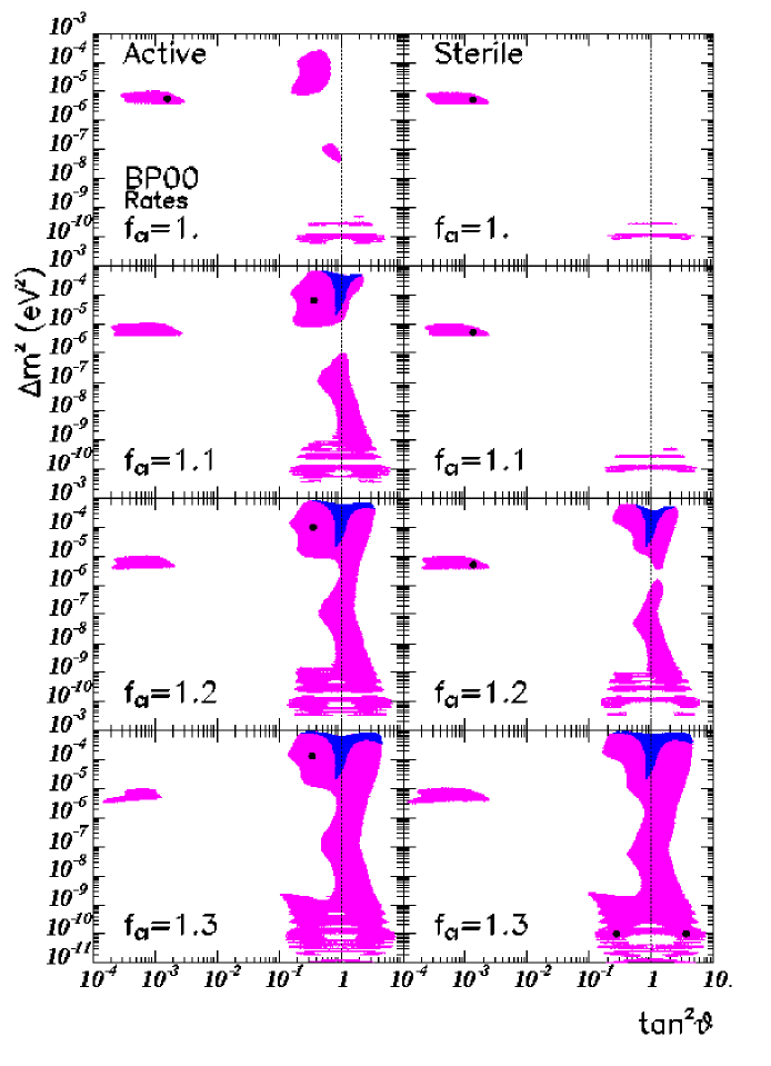
FIG. 4.: 99% CL regions allowed by the analysis of the experimental rates in GALLEX–GNO/SAGE, SK and Chlorine experiments, for BP00 fluxes, for different values of $f_{\rm Cl}$ and for oscillations into active (left panels) and sterile (right panels) neutrinos. The dots mark the position of the best-fit points in each panel. The effective GP solutions are marked as dark areas.

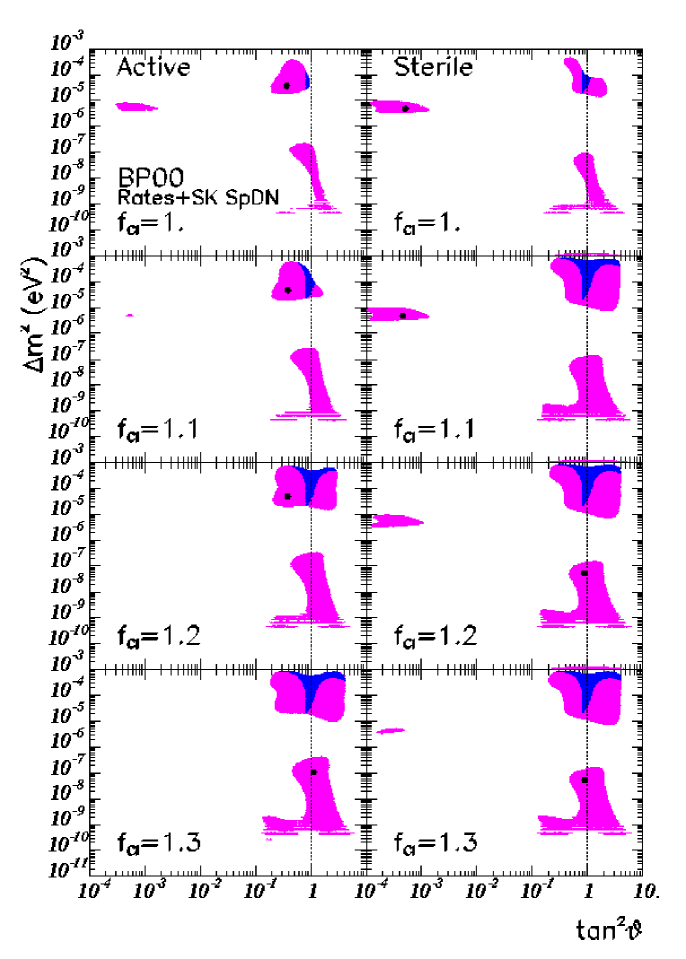
FIG. 5.: 99% CL regions allowed by the analysis of the three experimental rates and the SK day–night spectrum, for BP00 fluxes, for different values of $f_{\rm Cl}$ and for oscillations into active (left panels) and sterile (right panels) neutrinos. The dots mark the position of the best-fit points in each panel. The effective GP solutions are marked as dark areas.

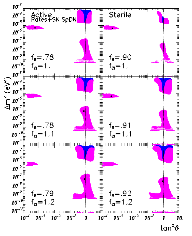
FIG. 6.: 99% CL regions allowed by the analysis of the three experimental rates and the SK day–night spectra for different values of $f_{\rm Cl}$ and $f_{\rm B}$, for oscillations into active neutrinos (left panels) and sterile neutrinos (right panels). The effective GP solutions are marked as dark areas. The dots mark the position of the best-fit points in each panel.

REFERENCES

- [1] V. Barger, S. Pakvasa, T.J. Weiler and K. Whisnant, Phys.Lett.B437 (1998) 107.
- [2] Y. Nomura and T. Yanagida, Phys.Rev. D59 (1999) 017303.
- [3] G. Altarelli and F. Feruglio, Phys.Lett. B439 (1998) 112.
- [4] E. Ma,Phys.Lett. B442 (1998) 238.
- [5] H. Fritzsch and Z. Xing, Phys. Lett. B372 (1998) 265.
- [6] H. Georgi and S.L. Glashow, Phys.Rev. D61 (2000) 097301.
- [7] R.N. Mohapatra and S. Nussinov, Phys.Lett. B441 (1998) 299.
- [8] R. Barbieri, L.J. Hall and A. Strumia, Phys.Lett. B445 (1999) 407.
- [9] C. Giunti, Phys.Rev. D59 (1999) 077301.
- [10] F. Vissani, hep-ph/9708483.
- [11] V.N. Gribov and B. Pontecorvo, Phys. Lett. B28 (1969) 493.
- [12] A. Acker, J.G. Learned, S. Pakvasa and T.J. Weiler, Phys. Lett B 298 (1993) 149.
- [13] P.F. Harrison, D.H. Perkins and W.G. Scott, Phys. Lett. B349 (1995) 137.
- [14] G. Conforto et al, Astropart. Phys. 5 (1996) 147.
- [15] A.J. Baltz, A.S. Goldhaber and M. Goldhaber, Phys. Rev. Lett. 81, (1998) 5730.
- [16] R. Crocker, R. Foot and R.R. Volkas, Phys. Lett. B465 (1999) 203; R. Foot, Phys. Lett. B483 (2000) 151.
- [17] S. Choubey, S. Goswami, N. Gupta and D.P. Roy (hep-ph/0103318).
- [18] M.C. Gonzalez-Garcia, C. Peña-Garay, Y. Nir, A.Yu. Smirnov, Phys. Rev.‘D63 (2001) 013007.
- [19] S.P. Mikheyev and A.Yu. Smirnov, Sov. Jour. Nucl. Phys. 42 (1985) 913; L. Wolfenstein, Phys. Rev. D17 (1978) 2369.
- [20] J. Bouchez et. al., Z. Phys. C32 (1986) 499. S.P. Mikheyev and A.Yu. Smirnov, ’86 Massive Neutrinos in Astrophysics and in Particle Physics, proceedings of the Sixth Moriond Workshop, edited by O. Fackler and J. Trn Thanh Vn (Editions Frontières, Gif-sur-Yvette, 1986), pp. 355; S.P. Mikheyev and A.Yu. Smirnov, Sov. Phys. Usp. 30 (1987) 759; A. Dar et. al. Phys. Rev. D 35 (1987) 3607; E.D. Carlson,Phys. Rev. D34 (1986) 1454; A.J. Baltz and J. Weneser, Phys. Rev. D35 (1987) 528 ; A.J. Baltz and J. Weneser, Phys. Rev. D37 (1988) 3364.
- [21] SAGE Collaboration, J.N. Abdurashitov et al., Phys. Rev. C60 (1999) 055801; V. Gavrin, talk at XIX International Conference on Neutrino Physics and Astrophysics, Sudbury, Canada, June 2000 (http://nu2000.sno.laurentian.ca).
- [22] GALLEX Collaboration, W. Hampel et al., Phys. Lett. B447 (1999) 127.
- [23] E. Belloti, talk at XIX International Conference on Neutrino Physics and Astrophysics, Sudbury, Canada, June 2000 (http://nu2000.sno.laurentian.ca).
- [24] S. Fukuda et al. [SuperKamiokande Collaboration], hep-ex/0103032.
- [25] B.T. Cleveland et al, Ap.J. 496 (1998) 505.
- [26] J.N. Bahcall and M. Pinsonneault, astro-ph/0010346.
- [27] M. Appolonio et al, Phys. Lett. B 466 (1999) 415.
- [28] M.C. Gonzalez-Garcia, P.C. de Holanda, C. Peña-Garay and J.W.F. Valle, Nucl. Phys. B573 (2000) 3; M.C. Gonzalez-Garcia, C. Peña-Garay, Nucl. Phys. Proc. Suppl. 91 (2000) 80 .
- [29] For a recent status report see A. Suzuki, Nucl. Phys. B (Proc. Suppl.) 77 (1999) 171.
- [30] L. Oberauer, Nucl. Phys. (Proc. Suppl.) 77 (1999) 48.