Bounds on Flavour Violating Parameters
in Supersymmetry

Abstract

We investigate the constraints on the flavour violating parameters from the decay $B\rightarrow X_{s}\gamma$, taking into account the interplay of the various sources of flavour violation in the unconstrained MSSM. We present a systematic leading logarithmic QCD analysis of these model-independent constraints, including contributions from gluinos, neutralinos, charginos, charged Higgs bosons and interferences between them. We show that two simple combinations of elements of the down squark mass matrix are stringently bounded over large parts of the parameter space where only weak assumptions on the hierarchical structure of the squark mass matrices are made. We also briefly analyse up to which values SUSY contributions, compatible with $B\rightarrow X_{s}\gamma$, can enhance the Wilson coefficient $C_{8}(m_{W})$, which plays an important role in the phenomenology of charmless hadronic $B$ decays.

I Introduction

Today supersymmetric models are given priority in the search for new physics beyond the standard model (SM). This is primarily suggested by theoretical arguments related to the hierarchy problem. Supersymmetry eliminates the sensitivity for the highest scale in the theory and, thus, stabilizes the low energy theory.

Flavour changing neutral current (FCNC) processes provide crucial guidelines for supersymmetry model building. In the so-called unconstrained minimal supersymmetric standard model (uMSSM) there are new sources for FCNC transitions. Besides the Cabibbo–Kobayashi–Maskawa (CKM)-induced contributions, there are generic supersymmetric contributions induced by flavour mixing in the squark mass matrices. The structure of the uMSSM does not explain the suppression of FCNC processes, which is observed in experiments; this is the crucial point of the well-known supersymmetric flavour problem. Within the framework of the MSSM there are at present three favoured supersymmetric models that solve the supersymmetric flavour problem by a specific mechanism through which the sector of supersymmetry breaking communicates with the sector accessible to experiments: in the minimal supergravity model (mSUGRA) [1], supergravity is the corresponding mediator; in the other two models, this is achieved by gauge interactions [2] and by anomalies [3]. Furthermore, there are other classes of models in which the flavour problem is solved by particular flavour symmetries [4].

Flavour violation thus originates from the interplay between the dynamics of flavour and the mechanism of supersymmetry breaking. FCNC processes therefore yield important (indirect) information on the construction of supersymmetric extensions of the SM and can contribute to the question of which mechanism ultimately breaks supersymmetry. The experimental measurements of the rates for these processes, or the upper limits set on them, impose in general a reduction of the large number and size of parameters in the soft supersymmetry-breaking terms present in these models. Among these processes, those involving transitions between first- and second-generation quarks, namely FCNC processes in the $K$ system, are considered as the most formidable tools to shape viable supersymmetric flavour models. Moreover, the tight experimental bounds on some flavour-diagonal transitions, such as the electric dipole moment of the electron and of the neutron, as well as $g-2$, help constraining soft terms inducing chirality violations.

Among neutral flavour transitions involving the third generation, the rare decay $B\rightarrow X_{s}\gamma$ is at present the most important one, as it is the only inclusive mode which is already measured [5]. The theoretical SM prediction, up to next-to-leading logarithmic (NLL) precision [6] for its branching ratio, is in agreement with the experimental data. Although the experimental errors are still rather large, this decay mode already allows for theoretically clean and rather stringent constraints on the parameter space of various extensions of the SM (see for example [7]).

Once more precise data from the B factories are available, this decay will undoubtedly gain efficiency in selecting the viable regions of the parameter space in the above classes of models; it may also help discriminating among the models that will be proposed by then.

In this paper we present a model-independent analysis of the decay $B\rightarrow X_{s}\,\gamma$, based on a LL-QCD calculation, where contributions from $W$-bosons, charged Higgs bosons, charginos, neutralinos and gluinos are systematically included. Former analyses in the unconstrained MSSM neglected QCD corrections and only used the gluino contribution to saturate the experimental bounds. Technically, the so-called mass insertion approximation (MIA) was used where the off-diagonal elements of the squark mass matrices are taken to be small and their higher powers neglected. As a consequence of this single insertion approximation, no correlations between different sources of flavour violation were taken into account. In this way, one arrived at ’order-of-magnitude bounds’ on the soft parameters [9, 10, 11]. In [12], the sensitivity of the bounds on the down squark mass matrix to radiative QCD corrections was analysed including the SM and the gluino contributions. The aim of the present paper is to extend this analysis to include the contributions from charged Higgs bosons, charginos and neutralinos and their interference effects, and even more important, the effects that result when several flavour violating parameters, i.e. several off-diagonal elements in the squark mass matrices, are switched on simultaneously. We anticipate that two simple combinations of matrix elements of the down squark mass matrix remain rather stringently bounded over large parts of the parameter space, in a general scenario where only relatively weak assumptions on pattern of the squark mass matrices are made.

Since there are different contributions to this decay, with different numerical impact on its rate, some of these flavour-violating terms may turn out to be poorly constrained. Thus, given the generality of such a calculation, it is convenient to rely on the mass eigenstate formalism, which remains valid even when some of the intergenerational mixing elements are large, and not to use the approximate mass insertion method, where the off-diagonal squark mass matrix elements are taken to be small and their higher powers neglected. In the latter approach the reliability of the approximation can only be checked a posteriori.

Finally, we note that the off-diagonal elements of the squark mass matrices can get constraints on completely different grounds, namely from the requirement of the absence of charge and colour breaking minima as well as from directions in the scalar potential which are unbounded from below (see [13] for a more detailed discussion). However, these bounds correspond to sufficient, but not necessary conditions for the stability of the standard vacuum, because it is possible that we live in a metastable vacuum, whose lifetime is longer than the age of the universe [14].

The paper is organized as follows: In section 2, we discuss the framework for the calculation of the branching ratio for $B\rightarrow X_{s}\gamma$. In section 3, we briefly recall the sources of flavour violation, encoded in the squark mass matrices. In section 4, we present the phenomenological analysis on the bounds on the flavour violating parameters. In section 5, we briefly explore up to which values SUSY contributions, allowed by $B\rightarrow X_{s}\gamma$, can enhance the Wilson coefficient $C_{8}(m_{W})$, which plays an important role in the phenomenology of charmless hadronic $B$ decays. In section 6 we give a short summary. In appendix A1, we state our conventions, while in appendix A2 we list the Wilson coefficients at the matching scale.

II Framework for calculating $B\rightarrow X_{s}\gamma$

A Hamiltonians

In the SM, rare $B$-meson decays are induced by one-loop diagrams in which $W$ bosons and up-type quarks propagate. The most important corrections to the decay amplitude for $b\to s\gamma$ are due to exchanges of gluons, which give rise to powers of the factor $L=\log(m_{b}^{2}/m_{W}^{2})$. It turns out that each of these logarithms is accompanied by at least one factor of $\alpha_{s}$. Since the two scales $m_{b}$ and $m_{W}$ are far apart, $L$ is a large number and these terms need to be resummed: at the leading logarithmic (LL) order, powers of $\alpha_{s}L$ are resummed; at the next-to-leading (NLL) order, also the terms of the form $\alpha_{s}\,(\alpha_{s}L)^{N}$ are systematically resummed. Thus, the contributions to the decay amplitude are classified according to

$$\quad(LL):\quad\quad G_{F}\,(\alpha_{s}L)^{N},\quad\quad(NLL):\quad G_{F}\,\alpha_{s}(\alpha_{s}L)^{N},\quad(N=0,1,...)$$ (1)

where $G_{F}$ is the Fermi constant. The resummation of these corrections is usually achieved by making use of the formalism of effective Hamiltonians, combined with renormalization group techniques. The effective Hamiltonian ${\cal H}_{eff}^{W}$, obtained by integrating out the top-quark and the $W$ boson, can be written as

$${\cal H}_{eff}^{W}=-\frac{4G_{F}}{\sqrt{2}}K_{tb}^{\phantom{\ast}}K_{ts}^{\ast}\sum_{i}C_{i}(\mu){\cal O}_{i}(\mu)\,.$$ (2)

The Wilson coefficients $C_{i}$ contain all dependence on the heavy degrees of freedom, whereas the operators ${\cal O}_{i}$ depend on light fields only. The operators relevant to $b\to s\gamma$ read

$$\begin{array}[]{llll}{\cal O}_{1}\,=&\!(\bar{s}\gamma_{\mu}T^{a}P_{L}c)\,(\bar{c}\gamma^{\mu}T_{a}P_{L}b)\,,&\\[5.16663pt] {\cal O}_{2}\,=&\!(\bar{s}\gamma_{\mu}P_{L}c)\,(\bar{c}\gamma^{\mu}P_{L}b)\,,&\\[5.16663pt] {\cal O}_{3}\,=&\!(\bar{s}\gamma_{\mu}P_{L}b)\sum_{q}(\bar{q}\gamma^{\mu}q)\,,&\\[5.16663pt] {\cal O}_{4}\,=&\!(\bar{s}\gamma_{\mu}T^{a}P_{L}b)\sum_{q}(\bar{q}\gamma^{\mu}T_{a}q)\,,&\\[5.16663pt] {\cal O}_{5}\,=&\!(\bar{s}\gamma_{\mu}\gamma_{\nu}\gamma_{\rho}P_{L}b)\sum_{q}(\bar{q}\gamma^{\mu}\gamma^{\nu}\gamma^{\rho}q)\,,&\\[5.16663pt] {\cal O}_{6}\,=&\!(\bar{s}\gamma_{\mu}\gamma_{\nu}\gamma_{\rho}T^{a}P_{L}b)\sum_{q}(\bar{q}\gamma^{\mu}\gamma^{\nu}\gamma^{\rho}T_{a}q)\,,&\\[5.16663pt] {\cal O}_{7}\,=&\!\displaystyle{\frac{e}{16\pi^{2}}}\,{\overline{m}}_{b}(\mu)\,(\bar{s}\sigma^{\mu\nu}P_{R}b)\,F_{\mu\nu}\,,\\[8.61108pt] {\cal O}_{8}\,=&\!\displaystyle{\frac{g_{s}}{16\pi^{2}}}\,{\overline{m}}_{b}(\mu)\,(\bar{s}\sigma^{\mu\nu}T^{a}P_{R}b)\,G^{a}_{\mu\nu}\,.\end{array}$$ (3)

The matrices $T^{a}$ ($a=1,...,8$) are $SU(3)$ colour generators and $P_{L,R}$ are left- and right-handed projection operators; $e$ and $g_{s}$ denote the electromagnetic and the strong coupling constants, respectively. Note that the $b$-quark mass is the relevant parameter that governs the chirality flip in the SM dipole operators ${\cal O}_{7}$ and ${\cal O}_{8}$. All eight operators are of dimension six. We anticipate that this is in contrast with the dipole operators induced by gluinos, where the helicity flip can be generated by the gluino mass instead of the $b$-quark mass, as we will see in more detail later. As a consequence, these dipole operators are effectively of dimension five.

A consistent SM calculation for $B\to X_{s}\gamma$ at LL (or NLL) precision requires three steps:

• a matching calculation of the full SM theory with the effective theory at the scale $\mu=\mu_{W}$ to order $\alpha_{s}^{0}$ (or $\alpha_{s}^{1}$) for the Wilson coefficients, where $\mu_{W}$ denotes a scale of order $m_{W}$ or $m_{t}$;

• a renormalization group treatment of the Wilson coefficients using the anomalous-dimension matrix to order $\alpha_{s}^{1}$ (or $\alpha_{s}^{2}$);

• a calculation of the operator matrix elements at the scale $\mu=\mu_{b}$ to order $\alpha_{s}^{0}$ (or $\alpha_{s}^{1}$), where $\mu_{b}$ denotes a scale of order $m_{b}$.

In supersymmetric models there are further contributions to the FCNC processes studied in this paper, i.e. the exchange of charged Higgs bosons and up-type quarks; of charginos and up-type squarks; of neutralinos and down-type squarks; and of gluinos and down-type squark. They all lead to $|\Delta(B)|=|\Delta(S)|=1$ effective magnetic and chromomagnetic operators (of ${\cal O}_{7}$-type, ${\cal O}_{8}$-type) and also to new four-quark operators.

Taking into account operators up to dimension six only, the effects of charginos, neutralinos and charged Higgs bosons can be matched onto the usual SM magnetic and chromomagnetic operators ${\cal O}_{7}$ and ${\cal O}_{8}$ and their primed counterparts

$$\begin{array}[]{llll}{\cal O}_{7}^{\prime}\,=&\!\displaystyle{\frac{e}{16\pi^{2}}}\,{\overline{m}}_{b}(\mu)\,(\bar{s}\sigma^{\mu\nu}P_{L}b)\,F_{\mu\nu}\,,&\quad{\cal O}_{8}^{\prime}\,=&\!\displaystyle{\frac{g_{s}}{16\pi^{2}}}\,{\overline{m}}_{b}(\mu)\,(\bar{s}\sigma^{\mu\nu}T^{a}P_{L}b)\,G^{a}_{\mu\nu}\,.\end{array}$$ (4)

We would like to stress that we do not work in the mSUGRA scenario. Therefore, a lot of the relations deduced in [8] do not hold anymore. The most important thing to notice is that in a general SUSY framework, there is no connection between the Yukawa couplings in the superpotential and the corresponding trilinear term in the soft potential. However, the contributions from charginos and charged Higgs bosons to the Wilson coefficients of the primed operators vanish also in the more general unconstrained MSSM if $m_{s}$ is put to zero (see eqs. (A32) and (A35)). This implies that for physical values of $m_{s}$ the chargino- and the charged Higgs boson contributions to the primed operators are small in scenarios in which $\tan\beta$ does not take extreme values. The neutralino contributions to both, the primed and unprimed operators are also unimportant, because their Wilson coefficients involve those entries of the squark mixing matrices $\Gamma_{DL}$ and $\Gamma_{DR}$, which also induce gluino contributions; the latter, which are proportional to $g_{s}^{2}$ therefore dominate the neutralino contributions which are proportional to $g_{2}^{2}$. We also found numerically that the neutralino contibutions are indeed rather inessential.

The fact that the operators generated by charged Higgs bosons, charginos and neutralinos can be matched onto the SM operators and their primed counterparts implies that the terms that get resummed at LL, show the same pattern as those listed in eq. (1); the Fermi constant appearing there is obviously replaced by a specific supersymmetric parameter for the chargino and neutralino contributions.

Matters are somewhat different for the gluino contribution ${\cal H}_{eff}^{\tilde{g}}$, as worked out in detail in [12]. At the amplitude level, terms of the form

• $(LL)$: $\quad\quad\alpha_{s}\,(\alpha_{s}L)^{N},$  $(NLL)$: $\quad\alpha_{s}\,\alpha_{s}(\alpha_{s}L)^{N}$,  $(N=0,1,...)$

are resummed, respectively at the leading and next-to-leading order. While ${\cal H}_{eff}^{\tilde{g}}$ is unambiguous, it is a matter of convention whether the $\alpha_{s}$ factors should be put into the definition of operators or into the Wilson coefficients. We follow the framework developed in ref. [12], where the distribution of the $\alpha_{s}$ factors was done in such a way that the anomalous dimension matrix systematically starts at order $\alpha_{s}$. We write the effective Hamiltonian ${\cal H}_{eff}^{\tilde{g}}$ in the form

$${\cal H}_{eff}^{\tilde{g}}=\sum_{i}C_{i,\tilde{g}}(\mu){\cal O}_{i,\tilde{g}}(\mu)+\sum_{i}\sum_{q}C_{i,\tilde{g}}^{q}(\mu){\cal O}_{i,\tilde{g}}^{q}(\mu)\,.$$ (5)

The index $q$ runs over all light quarks $q=u,d,c,s,b$. Among the operators contributing to the first part, there are dipole operators in which the chirality flip is induced by the $b$-quark mass:

$$\begin{array}[]{llll}{\cal O}_{7b,\tilde{g}}\,=&\!e\,g_{s}^{2}(\mu)\,{\overline{m}}_{b}(\mu)\,(\bar{s}\sigma^{\mu\nu}P_{R}b)\,F_{\mu\nu}\,,&{\cal O}_{7b,\tilde{g}}^{\prime}\,=&\!e\,g_{s}^{2}(\mu)\,{\overline{m}}_{b}(\mu)\,(\bar{s}\sigma^{\mu\nu}P_{L}b)\,F_{\mu\nu}\,,\\[8.61108pt] {\cal O}_{8b,\tilde{g}}\,=&\!g_{s}^{3}(\mu)\,{\overline{m}}_{b}(\mu)\,(\bar{s}\sigma^{\mu\nu}T^{a}P_{R}b)\,G^{a}_{\mu\nu}\,,&{\cal O}_{8b,\tilde{g}}^{\prime}\,=&\!g_{s}^{3}(\mu)\,{\overline{m}}_{b}(\mu)\,(\bar{s}\sigma^{\mu\nu}T^{a}P_{L}b)\,G^{a}_{\mu\nu}\,.\end{array}$$ (6)

As discussed in [12], there are also gluino-induced operators where the chirality violation is signalled by the charm quark mass (obtained by replacing ${\overline{m}}_{b}(\mu)$ by ${\overline{m}}_{c}(\mu)$) and operators where the chirality flip is induced by the gluino mass. The latter read

$$\begin{array}[]{llll}{\cal O}_{7\tilde{g},\tilde{g}}\,=&\!e\,g_{s}^{2}(\mu)\,(\bar{s}\sigma^{\mu\nu}P_{R}b)\,F_{\mu\nu}\,,&\quad{\cal O}_{7\tilde{g},\tilde{g}}^{\prime}\,=&\!e\,g_{s}^{2}(\mu)\,(\bar{s}\sigma^{\mu\nu}P_{L}b)\,F_{\mu\nu}\,,\\ &\\[-5.59721pt] {\cal O}_{8\tilde{g},\tilde{g}}\,=&\!g_{s}^{3}(\mu)\,(\bar{s}\sigma^{\mu\nu}T^{a}P_{R}b)\,G^{a}_{\mu\nu}\,,&\quad{\cal O}_{8\tilde{g},\tilde{g}}^{\prime}\,=&\!g_{s}^{3}(\mu)\,(\bar{s}\sigma^{\mu\nu}T^{a}P_{L}b)\,G^{a}_{\mu\nu}\,.\end{array}$$ (7)

At the LL-level, these operators could be absorbed into the operators given in eq. (6), when neglecting the small mixings effects from the gluino-induced four-Fermi operators with scalar or tensor Lorentz structure. However, as it is useful to separate the contributions where the chirality flip is induced by $m_{\tilde{g}}$, we do not perform this absorption. Notice that the operators in eq. (7) have dimension five, while the other operators are of dimension six. We also stress that unlike the other supersymmetric contributions, the primed gluino-induced operators are not suppressed compared with the unprimed ones. This is in strong contrast with the mSUGRA scenario, where the primed operators are stronlgy suppressed [8].

The contributions to the second part in eq. (5) are given by four-quark operators with vector, scalar and tensor Lorentz structure. As shown in ref. [12], the scalar and tensor operators mix at one loop into the six-dimensional magnetic and chromomagnetic ones. Therefore, they have to be included in principle in a LL calculation. As mentioned above, these mixings are numerically small and therefore not very important in practice.

For completeness we recall all Wilson coefficients at the matching scale $\mu_{W}$ in appendix A 2. The anomalous dimension matrix of the SM operators ${\cal O}_{1}$–${\cal O}_{8}$ and the evolution of the corresponding Wilson coefficients to the decay scale $\mu_{b}$ are well known and can be found in [6]. The evolution of the gluino-induced Wilson coefficients $C_{i,\tilde{g}}$ is given in ref. [12].

B Branching ratio

The decay width for $B\rightarrow X_{s}\gamma$ to LL precision is given by

$$\Gamma(B\to X_{s}\gamma)=\frac{m_{b}^{5}\,G_{F}^{2}\,|K_{tb}K_{ts}^{*}|^{2}\,\alpha}{32\pi^{4}}\ \left(\left|\hat{C}_{7}(\mu_{b})\right|^{2}+\left|\hat{C}^{\prime}_{7}(\mu_{b})\right|^{2}\right)\,,$$ (8)

where the auxiliary quantities $\hat{C}_{7}(\mu_{b})$ and $\hat{C}^{\prime}_{7}(\mu_{b})$ are defined as

$$\hat{C}_{7}(\mu_{b}) = C_{7}^{\rm{eff}}(\mu_{b})-\left[C_{7b,\tilde{g}}(\mu_{b})+\frac{1}{m_{b}}C_{7\tilde{g},\tilde{g}}(\mu_{b})\right]\,\frac{16\sqrt{2}\pi^{3}\alpha_{s}(\mu_{b})}{G_{F}\,K_{tb}K_{ts}^{*}}\,,$$ (9)

$$\hat{C}^{\prime}_{7}(\mu_{b}) = C_{7}^{\prime}(\mu_{b})\,-\left[C^{\prime}_{7b,\tilde{g}}(\mu_{b})+\frac{1}{m_{b}}C^{\prime}_{7\tilde{g},\tilde{g}}(\mu_{b})\right]\,\frac{16\sqrt{2}\pi^{3}\alpha_{s}(\mu_{b})}{G_{F}\,K_{tb}K_{ts}^{*}}\,,$$ (10)

where

$$C_{7}^{\rm{eff}}(\mu_{b})=C_{7}(\mu_{b})-\frac{1}{3}C_{3}(\mu_{b})-\frac{4}{9}C_{4}(\mu_{b})-\frac{20}{3}C_{5}(\mu_{b})-\frac{80}{9}C_{6}(\mu_{b})\,.$$ (11)

Note that we have neglected the small contributions from the operators ${\cal O}_{7c,\tilde{g}}$ and ${\cal O}_{7c,\tilde{g}}^{\prime}$. The branching ratio can be expressed as

$${\rm BR}(B\to X_{s}\gamma)=\frac{\Gamma(B\to X_{s}\gamma)}{\Gamma_{SL}}\,{\rm BR}_{SL}\,,$$ (12)

where ${\rm BR}_{SL}=(10.49\pm 0.46)\%$ is the measured semileptonic branching ratio. To the relevant order in $\alpha_{s}$, the semileptonic decay width is given by:

$$\Gamma_{SL}=\frac{m_{b}^{5}\,G_{F}^{2}\,|K_{cb}|^{2}}{192\pi^{3}}\,g\left(\frac{m_{c}^{2}}{m_{b}^{2}}\right)\,,$$ (13)

where the phase-space function $g(z)$ is $g(z)=1-8z+8z^{3}-z^{4}-12z^{2}\log z$.

Note that there is no systematic distinction between the pole mass $m_{b}$ and the corresponding running mass normalized at the scale $\mu_{b}$ in the LL approximation. To be specific, the mass parameters are always treated as pole masses in our numerical analysis.

III Squark Mass Matrices as New Sources of Flavour Violation

As advocated in the introduction, the aim of this paper is to provide a phenomenological analysis of the constraints on the flavour violating parameters in supersymmetric models with the most general soft terms in the squark mass matrices. As explained there, we work in the mass eigenstate formalism, which remains valid (in contrast to the mass insertion approximation) when the intergenerational mixing elements are not small.

A specification of the squark mass matrices usually starts in the super-CKM basis, in which the superfields are rotated in such a way that the mass matrices of the quark fields are diagonal. In this basis, the $6\times 6$ squared-mass matrix for the $d$-type squarks has the form

$${\cal M}_{d}^{2}\equiv\left(\begin{array}[]{cc}m^{2}_{\,d,\,LL}+F_{d\,LL}+D_{d\,LL}&\left(m_{\,d,\,LR}^{2}\right)+F_{d\,LR}\\[4.34857pt] \left(m_{\,d,\,LR}^{2}\right)^{\dagger}+F_{d\,RL}&\ \ m^{2}_{\,d,\,RR}+F_{d\,RR}+D_{d\,RR}\end{array}\right)\,.$$ (14)

For the $u$-type squarks we have

$${\cal M}_{u}^{2}\equiv\left(\begin{array}[]{cc}m^{2}_{\,u,\,LL}+F_{u\,LL}+D_{u\,LL}&\left(m_{\,u,\,LR}^{2}\right)+F_{u\,LR}\\[4.34857pt] \left(m_{\,u,\,LR}^{2}\right)^{\dagger}+F_{u\,RL}&\ \ m^{2}_{\,u,\,RR}+F_{u\,RR}+D_{u\,RR}\end{array}\right)\,.$$ (15)

In this basis, the $F$ terms (stemming from the superpotential) in the $6\times 6$ mass matrices ${\cal M}^{2}_{f}$ ($f=u,d$) are diagonal $3\times 3$ submatrices, reading $(F_{f\,RL}=F_{f\,LR}^{\dagger})$

$$(F_{d\,LR})_{ij}=-\mu(m_{d,i}\tan\beta)\,{{\mathchoice{\rm 1\mskip-4.0mul}{\rm 1\mskip-4.0mul}{\rm 1\mskip-4.5mul}{\rm 1\mskip-5.0mul}}}_{ij}\,,\,\,\,(F_{u\,LR})_{ij}=-\mu(m_{u,i}\cot\beta)\,{{\mathchoice{\rm 1\mskip-4.0mul}{\rm 1\mskip-4.0mul}{\rm 1\mskip-4.5mul}{\rm 1\mskip-5.0mul}}}_{ij}\,,$$ (16)

$$(F_{d\,LL})_{ij}=m^{2}_{d\,i}\,{{\mathchoice{\rm 1\mskip-4.0mul}{\rm 1\mskip-4.0mul}{\rm 1\mskip-4.5mul}{\rm 1\mskip-5.0mul}}}_{ij}\,,\,\,\,(F_{u\,LL})_{ij}=m^{2}_{u\,i}\,{{\mathchoice{\rm 1\mskip-4.0mul}{\rm 1\mskip-4.0mul}{\rm 1\mskip-4.5mul}{\rm 1\mskip-5.0mul}}}_{ij}\,.$$ (17)

Also the $D$-term contributions $D_{f\,LL}$ and $D_{f\,RR}$ to the squared-mass matrix are diagonal in flavour space:

$$D_{f\,LL,RR}=\cos 2\beta\,m_{Z}^{2}\left(T_{f}^{3}-Q_{f}\sin^{2}\theta_{W}\right){{\mathchoice{\rm 1\mskip-4.0mul}{\rm 1\mskip-4.0mul}{\rm 1\mskip-4.5mul}{\rm 1\mskip-5.0mul}}}_{3}\,.$$ (18)

Since present collider limits give indications that the squark masses are larger than those of the corresponding quarks, the largest entries in the squark mass matrices squared must come from the soft potential, directly linked to the mechanism of supersymmetry breaking. These contributions, denoted in (14) and (15) by $m^{2}_{\,f,\,LL}$, $m^{2}_{\,f,\,RR}$ and $m^{2}_{\,f,\,LR}$, are in general not diagonal in the super-CKM basis.

Further comments are in order. Because of $SU(2)_{L}$ invariance, $m^{2}_{\,u,\,LL}$ and $m^{2}_{\,d,\,LL}$ are related. In the super-CKM basis this relation reads $m^{2}_{\,u,\,LL}=Km^{2}_{d,LL}K^{\dagger}$, where $K$ denotes the CKM matrix. The off-diagonal $3\times 3$ block matrix $m_{\,f,\,LR}^{2}$ equals $A^{\,\ast}_{d}v_{d}$ for down-type and $A^{\,\ast}_{u}v_{u}$ for up-type squarks (the two vacuum expectation values are chosen to be real). They arise from the trilinear terms in the soft potential, namely $A_{d,ij}H_{d}\,{\widetilde{D}}_{i}{\widetilde{D}}_{j}^{c}$ and $A_{u,ij}H_{u}\,{\widetilde{U}}_{i}{\widetilde{U}}_{j}^{c}$. We stress that we do not assume the proportionality of these trilinear terms to the Yukawa couplings, as is done in the mSUGRA model. Furthermore, differently from $m^{2}_{\,f,\,LL}$ and $m^{2}_{\,f,\,RR}$, the off-diagonal $3\times 3$ matrix $m_{\,f,\,LR}^{2}$ is not hermitian.

Because all neutral gaugino couplings are flavour diagonal in the super-CKM basis and the mixing in the charged gaugino coupling to quarks and squarks is governed by the conventional CKM matrix, the flavour change through squark mass mixing is parametrized by the off-diagonal elements of the soft terms $m^{2}_{f,LL}$, $m^{2}_{f,RR}$, $m^{2}_{f,LR}$ in this basis.

The diagonalization of the two $6\times 6$ squark mass matrices ${\cal M}^{2}_{d}$ and ${\cal M}^{2}_{u}$ yields the eigenvalues $m_{\tilde{d}_{k}}^{2}$ and $m_{\tilde{u}_{k}}^{2}$ ($k=1,...,6$). The corresponding mass eigenstates, $\tilde{u}_{k}$ and $\tilde{d}_{k}$ ($k=1,...,6$) are related to the fields in the super-CKM basis, $\tilde{u}_{Lj}$, $\tilde{u}_{Rj}$ and $\tilde{d}_{Lj}$, $\tilde{d}_{Rj}$, ($j=1,...,3$) as

$$\tilde{u}_{L,R}=\Gamma^{\dagger}_{UL,R}\,\tilde{u}\,,\hskip 28.45274pt\tilde{d}_{L,R}=\Gamma^{\dagger}_{DL,R}\,\tilde{d}\,,$$ (19)

where the four matrices $\Gamma_{UL,R}$ and $\Gamma_{DL,R}$ are $6\times 3$ mixing matrices.

IV Phenomenological Analysis

Our phenomenological analysis is based on a complete LL QCD calculation within the unconstrained MSSM; it is done in two parts:

• In the first part, we try to derive bounds on the off-diagonal elements of the squark mass matrices by switching on only one of these elements at a time. We include, however, all new physics contributions (chargino, neutralino, charged Higgs bosons, gluino) in the analysis. We show that only those parameters get stringently bounded by $B\to X_{s}\gamma$, which can generate contributions to the five-dimensional gluino-induced dipole operators ${\cal O}_{7\tilde{g},\tilde{g}}$ and ${\cal O}^{\prime}_{7\tilde{g},\tilde{g}}$.

• In the second part of our analysis we investigate whether the bounds obtained in the first part remain stable, if all off-diagonal elements, which induce the decay $B\rightarrow X_{s}\gamma$, are varied simultaneously. We anticipate that the bounds on the individual off-diagonal elements get lost, because in this case various combinations of off-diagonal elements can contribute (with opposite sign) to the Wilson coefficients of the five-dimensional dipole operators. In the scenarios we discuss below, it is, however, possible to constrain certain simple combinations of off-diagonal elements of the down squark mass matrices, provided $\tan\beta$ and $\mu$ are not very large.

A General comments

In order to analyse the implications of $B\to X_{s}\gamma$ on the flavour violating soft parameters in the squark mass matrices, we choose some specific scenarios that are characterized by the values of the parameters

$$\mu,\quad M_{H^{-}},\quad\tan\beta,\quad M_{\rm{susy}},\quad m_{\tilde{g}}.$$ (20)

We regard this as reasonable, because we expect that these input parameters, which are unrelated to flavour physics, will be fixed from flavour conserving observables in the next generations of high energy experiments (provided low energy SUSY exists). Note that the common SUSY scale, $M_{\rm{susy}}$, fixes in our scenarios the general soft squark mass scale $m_{\tilde{q}}$ (see eqs. (22,23)) and the first diagonal element of the chargino mass matrix $M_{2}$ (see eq. (A4)).

The parameters are chosen as follows: for $M_{\rm{susy}}$ we choose the three values $M_{\rm{susy}}=300,500,1000\,GeV$, while for $\tan\beta$ we use the values $\tan\beta=2,10,30,50$. For the gluino mass, characterized by $x=m^{2}_{\tilde{g}}/M^{2}_{\rm{susy}}$, we take $x=0.3,0.5,1,2$. Unless otherwise stated, the $\mu$ parameter and the mass of the charged Higgs boson $M_{H^{-}}$ are fixed to be $\mu=300\,GeV$ and $M_{H^{-}}=300\,GeV$.

While in the first part of our analysis we set, following ref.[9], all diagonal soft entries in $m^{2}_{\,d,\,LL}$, $m^{2}_{\,d,\,RR}$, and $m^{2}_{\,u,\,RR}$ equal to the common soft squark mass scale $m^{2}_{\tilde{q}}$, we relax this condition in the second part of our analysis.

We point out that the present bound on the mass of the lightest neutral Higgs boson requires a non-vanishing mixing $(m^{2}_{u,LR})_{33}$ among the stop-squarks. For our choices of the parameters, the MSSM bound coincides with the bound on the SM Higgs boson.

We note that there are two contributions to the stop-squark mixing, namely the ‘soft’ contribution $(m^{2}_{u,LR})_{33}$ and the $F$-term contribution ($-\mu\,m_{t}\,\cot\beta$). In a general unconstrained MSSM, the soft contribution does not scale with $m_{t}$. However, following common notation, we parametrize the stop mixing term in ${\cal M}_{u}^{2}$ (see eq. (15)) as

$$X_{t}\,m_{t}=(m^{2}_{u,LR})_{33}\,-\mu m_{t}\cot\beta\,.$$ (21)

We fix the stop mixing parameter $X_{t}$ such that the mass of the lightest Higgs boson is at least $115\,GeV$ to assure that the present Higgs bound is fulfilled in our analysis. We use the program FeynHiggsFast [18] which determines the Higgs boson mass approximately taking into account the complete one- and two-loop QCD corrections, the effects of the running top mass and of the Yukawa term for the light Higgs boson. The input parameters of the FeynHiggsFast program, are $\tan\beta$, the diagonal entries of the stop and the sbotton squark mass matrix, $M^{2}_{\tilde{t}_{L}}$, $M^{2}_{\tilde{t}_{R}}$, $M^{2}_{\tilde{b}_{L}}$, and $M^{2}_{\tilde{b}_{R}}$, the stop and the sbotton mixing parameters, $X_{t}$ and $X_{b}$, the top mass $m_{t}$, the parameter $\mu$ and the charged Higgs boson mass. For $\tan\beta=10$ we choose the following values for $X_{t}$ in dependence of the parameter $M_{{\rm susy}}$: $(M_{\rm{susy}},X_{t})=(300\,GeV,470\,GeV)$; $(500\,GeV,750\,GeV)$; $(1000\,GeV,1200\,GeV)$. (For $\mu=300\,GeV$ and $X_{b}=0$ we find Higgs boson masses of $115.2\,GeV$, $119.9\,GeV$ and $121.1\,GeV$, respectively.) The dependence of the Higgs boson mass on the parameters $\mu$ or $X_{b}$ is rather small within our parameter scenarios. Also for the $\tan\beta=30$ and $50$ scenarios we use the same values of $X_{t}$ for our convenience. In these cases the chosen $X_{t}$ values imply slightly higher Higgs boson masses. We also note that within our choice of parameters, the low $\tan\beta$ scenario, with $\tan\beta=2$, already gets excluded by the bound on the Higgs boson mass.

B First part of analysis

In this part of the analysis only one off-diagonal entry in the soft part of the squark mass matrices is different from zero. We further assume (as in ref. [9]) that all diagonal soft entries in $m^{2}_{\,d,\,LL}$, $m^{2}_{\,d,\,RR}$, and $m^{2}_{\,u,\,RR}$ are set to be equal to the common value $m_{\tilde{q}}^{2}=M^{2}_{\rm{susy}}$. Then we normalize the off-diagonal elements to $m_{\tilde{q}}^{2}$,

$$\delta_{f,LL,ij}=\frac{(m^{2}_{\,f,\,LL})_{ij}}{m^{2}_{\tilde{q}}}\,,\hskip 28.45274pt\delta_{f,RR,ij}=\frac{(m^{2}_{\,f,\,RR})_{ij}}{m^{2}_{\tilde{q}}}\,,\hskip 28.45274pt(i\neq j)$$ (22)

$$\delta_{f,LR,ij}=\frac{(m^{2}_{\,f,\,LR})_{ij}}{m^{2}_{\tilde{q}}}\,,\hskip 28.45274pt\delta_{f,RL,ij}=\frac{(m^{2}_{\,f,\,LR})^{\dagger}_{ij}}{m^{2}_{\tilde{q}}}\,.\phantom{\hskip 28.45274pt(i\neq j)}$$ (23)

We recall that the matrix $m_{u,LL}$ cannot be specified independently; $SU(2)_{L}$ gauge invariance implies that $m_{u,LL}=Km_{d,LL}K^{\dagger}$, where $K$ is the CKM matrix. We also note that our $\delta$-quantities only include the soft parts of the matrix elements of the squark mass matrices, while in ref. [9] also the $F$-term contributions are included in the definition of the $\delta$-quantities.

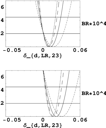
FIG. 1.: Dependence of $BR(B\rightarrow X_{s}\gamma)$ on $\delta_{d,LR,23}$. In the upper frame, only SM and gluino contributions are considered. In the lower frame, the additional contributions from chargino, charged Higgs boson and neutralino are included. The horizontal lines denote the experimental limits. The different lines correspond to different values of $x=m^{2}_{\tilde{g}}/m^{2}_{\tilde{q}}$: 0.3 (short-dashed line), 0.5 (long-dashed line), 1 (solid line), and 2 (dot-dashed line). The other parameters are $\mu=300\,GeV$, $\tan\beta=10$, $M_{H^{-}}=300\,GeV$, $M_{\rm{susy}}=500\,GeV$.

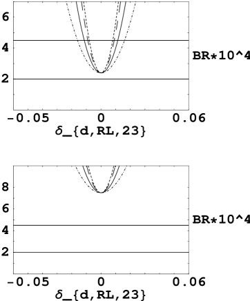
FIG. 2.: Same as in fig. 1 when $\delta_{d,RL,23}$ is the only non-zero off-diagonal squark mass entry.

In figs. 1 and 2, we show the dependence of the branching ratio of $B\rightarrow X_{s}\,\gamma$ on the flavour-violating parameters $\delta_{d,LR,23}$ and $\delta_{d,RL,23}$, respectively. The upper frame in each figure is borrowed from [12], i.e. we consider only SM and gluino contributions. As $\delta_{d,LR,23}$ and $\delta_{d,RL,23}$ generate the five-dimensional dipole operators ${\cal O}_{7\tilde{g},\tilde{g}}$ and ${\cal O}^{\prime}_{7\tilde{g},\tilde{g}}$, it is not surprising that they get stringently bounded. We should note that at this level of the analysis there is no dependence of these bounds on $\mu$ or $\tan\beta$. Such a dependence could result from the term $(F_{d,LR})_{33}$, but only when $\delta_{d,LL,23}$ and $\delta_{d,RR,23}$ are turned on. We will discuss this point in more detail at the end of this section and in the second part of our analysis. In the lower frame of figs. 1 and 2, we also include the contributions from charginos, charged Higgs bosons and neutralinos. Comparing the branching ratio in the two frames at $\delta_{d,LR,23}=0$ and $\delta_{d,RL,23}=0$ (which corresponds to switching off the gluino contribution), one concludes that the combined contribution from charginos, neutralinos and charged Higgs bosons is of the same order as the SM contribution. A detailed investigation shows that the neutralino contribution is negligible, while the contributions from the chargino and charged Higgs boson are similar in magnitude; both interfere constructively with the SM contributions for the specific choice of parameters. However, as the gluino yields, intrinsically, the dominant contribution by far, the bounds $\delta_{d,LR,23}$ and $\delta_{d,RL,23}$ are only marginally modified by chargino, neutralino and charged Higgs boson contributions. A comment concerning the different shapes of the curves in figs. 1 and 2 is in order. In fig. 2, with non-vanishing $\delta_{d,RL,23}$, the gluino contribution is induced by the primed-type operator ${\cal O}^{\prime}_{7\tilde{g},\tilde{g}}$ and therefore does not interfere with the contributions from the other particles, as these induce unprimed operators in the first place. In contrast, in fig. 1, which shows the case of non-zero $\delta_{d,LR,23}$, the gluino contribution is of the unprimed type and therefore interferes with the other contributions.

We also tried to derive analogous bounds on $\delta_{d,LL,23}$, $\delta_{d,RR,23}$, $\delta_{u,LR,23}$, $\delta_{u,RL,23}$, $\delta_{u,RR,23}$ and also on $\delta_{u,LR,33}$ and $\delta_{u,LR,22}$. In the chargino sector the latter diagonal elements, together with the usual CKM mechanism, also can induce flavour violation. The parameters of the up-squark mass matrix give rise to chargino contributions that lead only to dimension six dipole operators, which inherently are not very large. For our choices of $\mu$, $M_{\rm{susy}}$ and $\tan\beta$, this was confirmed numerically. Therefore, no stringent bounds are obtained for the soft parameters in the up-squark mass matrix. The remaining parameters of the down-squark mass matrix, i.e. $\delta_{d,LL,23}$ and $\delta_{d,RR,23}$, play an interesting role. They not only generate contributions to the six-dimensional operators in (6), but, together with the chirality changing term $(F_{d,LR})_{33}$, they also induce contributions to the five-dimensional gluino operators in (7). For the values of $\mu$ and $\tan\beta$ used in our analysis, the coefficients of the five-dimensional operators turn out to be rather small. Thus, no stringent bounds on $\delta_{d,LL,23}$ and $\delta_{d,RR,23}$ are obtained.

Summarizing the first part of our analysis, we conclude that $\delta_{d,LR,23}$ and $\delta_{d,RL,23}$ are the only parameters that get significantly constrained by the measurement of the branching ratio of $B\rightarrow X_{s}\gamma$.

C Second part of analysis

We now explore the problem of whether the separate bounds on $\delta_{d,LR,23}$ and $\delta_{d,RL,23}$, obtained in the first part, remain stable if the various soft parameters are varied simultaneously. The analysis is based on the assumption that the soft terms in the squark mass matrices have the hierarchical structure that the diagonal entries in $m^{2}_{\,d,\,LL}$, $m^{2}_{\,d,\,RR}$, and $m^{2}_{\,u,\,RR}$ are larger than the off-diagonal matrix elements (including $m^{2}_{\,d,\,LR}$ and $m^{2}_{\,u,\,LR}$). In contrast to the first part of the analysis, we will allow for a non-degeneracy of the diagonal elements in the matrices $m^{2}_{\,d,\,LL}$, $m^{2}_{\,d,\,RR}$, and $m^{2}_{\,u,\,RR}$. To implement this, we define $\delta$-quantities in addition to those in eqs. (22) and (23), which parametrize this non-degeneracy:

$$\delta_{f,LL,ii}=\frac{(m^{2}_{\,f,\,LL})_{ii}-m^{2}_{\tilde{q}}}{m^{2}_{\tilde{q}}}\,,\hskip 28.45274pt\delta_{f,RR,ii}=\frac{(m^{2}_{\,f,\,RR})_{ii}-m^{2}_{\tilde{q}}}{m^{2}_{\tilde{q}}}\,,$$ (24)

Unless otherwise stated, the diagonal $\delta$-parameters (in eq. (24)) are varied in the interval $[-0.2,0.2]$. On the other hand, the off-diagonal ones (in eqs. (22) and (23)) are varied in the interval $[-0.5,0.5]$, by use of a Monte Carlo program. There are, however, two exceptions. First, we do not vary those off-diagonal $\delta$’s with an index $1$; the latter $\delta$’s we set to zero, since they are severely constrained by kaon decays (see for example [9]). Second, as mentioned earlier, also $(m^{2}_{u,LR})_{33}$ is not varied, but fixed such that the mass of the lightest neutral Higgs boson gets heavy enough to be compatible with experimental bounds.

In our Monte Carlo analysis we plot those events, corresponding to $2.0\times 10^{-4}\leq BR(B\rightarrow X_{s}\gamma)\leq 4.5\times 10^{-4}$, which is the range allowed by the CLEO measurement. Note that we do not include recent preliminary data [5] in our analysis. Furthermore, we have made sure that our events correspond to squark masses that are real and lie above $150\,GeV$. The dependence of the bounds on this specific choice is discussed below.

FIG. 3.: Contours in the $\delta_{d,LR,23}$ - $\delta_{d,RL,23}$ plane. In the left frame, $\delta_{d,LR,23}$ and $\delta_{d,RL,23}$ are the only flavour-violating parameters. In the right frame, we allow also for non-vanishing $\delta_{d,LL,23}$ and $\delta_{d,RR,23}$. We only consider SM and gluino contributions and the other parameters are $\mu=300\,GeV$, $\tan\beta=10$, $M_{\rm{susy}}=500\,GeV$ and $x=1$.

We start with the following parameter set: $\mu=300\,GeV$, $M_{H^{-}}=300\,GeV$, $\tan\beta=10$, $M_{\rm{susy}}=500\,GeV$, $x=m_{\tilde{g}}^{2}\,/\,M_{\rm{susy}}^{2}=1$ and $X_{t}=750\,GeV$. In fig. 3, we only consider SM and gluino contributions. In the left frame we present the constraints on $\delta_{d,LR,23}$ and $\delta_{d,RL,23}$ when these are the only flavour-violating soft parameters; the diagonal $\delta$-parameters defined in eq. (24) are also switched off. As expected from the first part of our analysis, stringent constraints are obtained. The hole inside the dotted area represents values of $\delta_{d,LR,23}$ and $\delta_{d,RL,23}$ for which the branching ratio is too small to be compatible with the measurements. In the right frame we investigate interference effects that arise when $\delta_{d,LL,23}$ and $\delta_{d,RR,23}$ are switched on in addition to $\delta_{d,LR,23}$, $\delta_{d,RL,23}$. All of them are varied between $\pm 0.5$. From fig. 3 we find that the bounds on $\delta_{d,LR,23}$ and $\delta_{d,RL,23}$ cannot be softened significantly by non-zero values of $\delta_{d,LL,23}$ and $\delta_{d,RR,23}$, although these $\delta$-parameters, which individually give rise to six-dimensional operators, generate five-dimensional operators through the interplay with the $F$-term $(F_{d,LR})_{33}$. As already discussed in the first part of the analysis, for moderate values of $\mu$ and $\tan\beta$, the contribution to the Wilson coefficient of the five-dimensional operator is rather small.

FIG. 4.: Contours in the $\delta_{d,LR,23}$ - $\delta_{d,RL,23}$ plane, where $\delta_{d,LR,23}$, $\delta_{d,RL,23}$, $\delta_{d,LL,23}$ and $\delta_{d,RR,23}$ are the only flavour-violating parameters; $\delta_{d,LR,22}$, $\delta_{d,LR,33}$ are also non-vanishing. We only include SM and gluino contributions; the other parameters are $\mu=300\,GeV$, $\tan\beta=10$, $M_{\rm{susy}}=500\,GeV$ and $x=1$.

The full power of the interference effects from different sources of flavour violation is depicted in fig. 4, where we allow not only for non-zero $\delta_{d,LR,23}$, $\delta_{d,RL,23}$, $\delta_{d,LL,23}$ and $\delta_{d,RR,23}$ but also for non-vanishing $\delta_{d,LR,22}$, $\delta_{d,LR,33}$. All these parameters are varied between $\pm 0.5$. As can be seen, the bounds on $\delta_{d,LR,23}$ and $\delta_{d,RL,23}$ get destroyed dramatically. The reason is that there are now new contributions to the five-dimensional dipole operators. As an example, the combined effect of $\delta_{d,LR,33}$ and $\delta_{d,LL,23}$ leads to a contribution to the Wilson coefficient of the operator ${\cal O}_{7\tilde{g},\tilde{g}}$. The sign of this contribution can be different from the one generated by $\delta_{d,LR,23}$. As a consequence, the bound on $\delta_{d,LR,23}$ gets weakened. To illustrate this more quantitatively, we assume for the moment that there are only these two sources that can generate ${\cal O}_{7\tilde{g},\tilde{g}}$, i.e. we switch off the other $\delta$-quantities. If $\delta_{d,LR,23}$ is larger than the individual bound from the first part of the analysis, it is necessary that the product of $\delta_{d,LR,33}$ and $\delta_{d,LL,23}$ is also relatively large; only in this case can the two sources lead to a branching ratio compatible with experiment. This feature is illustrated in fig. 5; only values of $\delta_{d,LR,23}$ and values of $\delta_{d,LR,33}\cdot\delta_{d,LL,23}$ which are strongly correlated lead to an acceptable branching ratio.

FIG. 5.: The parameters $\delta_{d,LR,23}$ and $\delta_{d,LR,33}\cdot\delta_{d,LL,23}$, which are compatible with the data on $B\to X_{s}\gamma$ are shown by dots. Values lying on the solid line lead to a vanishing contribution of the five-dimensional operator ${\cal O}_{7\tilde{g},\tilde{g}}$ in the MIA. See text. We only switch on SM and gluino contributions; the other parameters are $\mu=300\,GeV$, $\tan\beta=10$, $M_{\rm{susy}}=500\,GeV$ and $x=1$.

As clearly visible from fig. 5, the correlation between the two sources for ${\cal O}_{7\tilde{g},\tilde{g}}$, is essentially linear. This implies that the linear combination

$$\delta_{d,LR,23}+f\delta_{d,LR,33}\cdot\delta_{d,LL,23}$$ (25)

gets constrained, if $f$ is chosen appropriately. Stated differently, the Wilson coefficient of the operator ${\cal O}_{7\tilde{g},\tilde{g}}$ is essentially proportional to the combination (25). This implies in turn that for the values of the parameters we are using at the moment ($\mu=300\,GeV$, $M_{H^{-}}=300\,GeV$, $\tan\beta=10$ $M_{\rm{susy}}=500\,GeV$, $x=m_{\tilde{g}}^{2}\,/\,M_{\rm{susy}}^{2}=1$, $X_{t}=750\,GeV$), the Wilson coefficient is well approximated by its double mass insertion expression. The coefficient $f$, which can be read off from this expression, depends on the parameter $x=m_{\tilde{g}}^{2}/M^{2}_{\rm{susy}}$ and reads

$$f(x)=\frac{1+9x-9x^{2}-x^{3}+6x(1+x)\log x}{(1-x)[5x^{2}-4x-1-2x(x+2)\log x]}\,.$$ (26)

The numerical values of $f(x)$ for some values of $x$ read $0.74$ for $x=0.3$, $0.68$ for $x=0.5$, $0.60$ for $x=1.0$ and $0.52$ for $x=2.0$, respectively.

The solid line in fig. 5 represents pairs ($\delta_{d,LR,23}$, $\delta_{d,LR,33}\cdot\delta_{d,LL,23}$) for which the combination in eq. (25) is zero. The points scattered around this line therefore represent Monte Carlo events for which this combination is small. We now turn back to the scenario of fig. 4 in which all the parameters $\delta_{d,LR,23}$, $\delta_{d,RL,23}$, $\delta_{d,LL,23}$, $\delta_{d,RR,23}$, $\delta_{d,LR,22}$, $\delta_{d,LR,33}$ are varied simultaneously. In this case, the linear combinations

$$LC_{1} = \delta_{d,RL,23}+f(x)\delta_{d,RR,23}\cdot\delta_{d,RL,33}+f(x)\delta_{d,RL,22}\cdot\delta_{d,LL,23},$$ (27)

$$LC_{2} = \delta_{d,LR,23}+f(x)\delta_{d,LR,22}\cdot\delta_{d,RR,23}+f(x)\delta_{d,LL,23}\cdot\delta_{d,LR,33},$$ (28)

are expected to get constrained.

In fig. 6 we show the allowed region for $LC_{1}$ and $LC_{2}$. There, we allow all non-diagonal $\delta$-parameters to vary between $\pm 0.5$. In addition, we also allow for non-equal diagonal soft entries, by varying the parameters $\delta_{f,LL,ii}$ and $\delta_{f,RR,ii}$ between $\pm 0.2$. With the latter choice we still guarantee the hierarchy between diagonal and off-diagonal entries, but we get rid of the unnatural assumption of degenerate diagonal entries. In the left frame, we include only SM and gluino contributions. We find that the linear combinations $LC_{1}$ and $LC_{2}$ indeed get stringently bounded.

FIG. 6.: Contours in the $LC_{1}$-$LC_{2}$ plane with $\delta_{d,LR,23}$, $\delta_{d,RL,23}$, $\delta_{d,LL,23}$, $\delta_{d,RR,23}$, $\delta_{d,LR,22}$, $\delta_{d,LR,33}$, $\delta_{u,LR,23}$, $\delta_{u,RL,23}$, $\delta_{u,LL,23}$, $\delta_{u,RR,23}$, and $\delta_{u,LR,22}$ all non-vanishing. In the left frame, we consider only SM and gluino contributions whereas in the right frame we also include chargino, charged Higgs boson and neutralino contributions. The values of the other parameters are $\mu=300\,GeV$, $\tan\beta=10$, $M_{H^{-}}=300\,GeV$, $M_{\rm{susy}}=500\,GeV$ and $x=1$.

In the right frame of fig. 6 we test the resistance of these bounds when the additional contributions (i.e., those from charginos, charged Higgs bosons and neutralinos) are turned on. In this case also $\delta_{u,LR,23}$, $\delta_{u,RL,23}$, $\delta_{u,LL,23}$, $\delta_{u,RR,23}$ and $\delta_{u,LR,22}$ are varied in the range $\pm 0.5$. We find that the bound on $LC_{1}$ remains unchanged, while the one on $LC_{2}$ gets somewhat weakened. This feature is expected, because charginos and charged Higgs bosons contribute to unprimed operators at first place. At this point we should stress that these plots were obtained by choosing the renormalization scale $\mu_{b}=4.8\,GeV$ and by requiring all squark masses to be larger than $150\,GeV$. We checked that the bounds on $LC_{1}$ and $LC_{2}$ remain practically unchanged when the renormalization scale is varied between $2.4\,GeV$ and $9.6\,GeV$; they are also insensitive to the value of the required minimal squark mass, as we found by changing $m_{\rm{squark\,min}}$ from $150\,GeV$ to $100\,GeV$ or $250\,GeV$. Moreover, we also checked whether the restriction to $\mu=+300$ $GeV$ scenario is too severe: we redid the complete analysis for $\mu=-300\,GeV$ and confirmed that ther are no differences between the results of these two choices.

Two remarks are in order: First, one might wonder why we did not include terms like $\delta_{d,RR,33}\cdot\delta_{d,LR,23}$ in $LC_{1}$ and $LC_{2}$, which would result into more complicated combinations. As we are allowing for nonequal diagonal soft entries, these terms give in principle additional contributions to the five dimensional operators. However, as the diagonal $\delta$-parameters are only varied between $\pm 0.2$, their influence on the Wilson coefficients is numerically small. For this reason, the simpler combinations $LC_{1}$ and $LC_{2}$, defined in eqs. (28), are sufficiently constrained and we prefer to give bounds on these quantities.
Second, if we got rid of the hierarchy of diagonal and off-diagonal entries in the squark mass matrices, stringent bounds on the simple combinations $LC_{1}$ and $LC_{2}$ certainly would no longer exist, simply because there would then be more contributions to the five-dimensional operators of similar magnitude. In this case, however, the $full$ Wilson coefficients of the five-dimensional operators still would be stringently constrained by the experimental data on $B\to X_{s}\gamma$. Unfortunately, in this case not much information can be extracted for the individual soft parameters or simple combinations thereof.

Finally, we extend our analysis to other values of the input parameters. So far, we found that the combinations $LC_{1}$ and $LC_{2}$ (see eqs. (28)) are stringently bounded in the scenario characterized by the input values $\mu=300\,GeV$, $M_{H^{-}}=300\,GeV$, $\tan\beta=10$, $M_{\rm{susy}}=500\,GeV$, $x=m_{\tilde{g}}^{2}\,/\,M_{\rm{susy}}^{2}=1$ and $X_{t}=750\,GeV$. It is conceivable that the bounds on $LC_{1}$ and $LC_{2}$ can get considerably weakened in other scenarios. Therefore, we analyse the bounds on the soft parameters within the following parameter sets: ($M_{\rm{susy}},X_{t}$) $=$ $(300\,GeV,470\,GeV)$, $(500\,GeV,750\,GeV)$, $(1000\,GeV,1200\,GeV)$. For $\tan\beta$ we explore the values: $\tan\beta=10,\,30,\,50.$ Furthermore, the gluino mass $m_{\tilde{g}}$ is varied over the values $x=m_{\tilde{g}}^{2}\,/\,M_{\rm{susy}}^{2}=0.3\,,\,0.5\,,\,1\,,\,2$.

FIG. 7.: $LC_{1}$ versus $LC_{2}$ in the $x=1$ scenario. Vertically we vary the parameter $M_{{\rm susy}}$ from $M_{{\rm susy}}=1000\,GeV$  in the first line, via $M_{{\rm susy}}=500\,GeV$  in the second to $M_{{\rm susy}}=300\,GeV$  in the last. Horizontally we vary $\tan\beta$ from $10$ via $30$ to $50$. The values of the other parameters are $\mu=300\,GeV$ and $M_{H^{-}}=300\,GeV$. All contributions are switched on.

Surprisingly, the constraints on $LC_{1}$ and $LC_{2}$ are completely stable over large parts of the parameter space. Within the $\tan\beta=10$ scenario the bounds are essentially unchanged if the other two parameters $M_{{\rm susy}}$ and $x$, are varied over the complete range of values given above. For example, the independence from the parameter $M_{{\rm susy}}$ within this scenario can be read off from the comparison of frames in the first vertical line in fig. 7.

However, fig. 7 also illustrates that the bounds get significantly weakened or even lost when $\tan\beta$ values as large as $30$ (second vertical line) or $50$ (third vertical line) are chosen. This effect gets enhanced when the general mass scale $m_{\tilde{q}}$ in the squark mass matrices decreases with the parameter $M_{\rm susy}$.

FIG. 8.: The left frame shows the bounds on $LC_{1}$ and $LC_{2}$ in a $\tan\beta=50$ scenario, which are relatively weak. In the right frame we put $(F_{d,LR})_{33}=0$. See text. The other parameters are $\mu=300\,GeV$, $M_{H^{-}}=300\,GeV$, $M_{\rm{susy}}=500\,GeV$ and $x=1$. All contributions are switched on.

FIG. 9.: The left frame shows bounds on $LC_{1}$ and $LC_{2}$ for a scenario with $\mu=900\,GeV$ and $\tan\beta=10$. The right frame shows the corresponding bounds obtained with $\mu=150\,GeV$ and $\tan\beta=30$. The other parameters in both frames are chosen to be $M_{H^{-}}=300\,GeV$, $M_{\rm{susy}}=500\,GeV$ and $x=1$. All contributions are switched on. See text.

There are two main reasons why the bounds get weakened in these scenarios. First, in the large $\tan\beta$ regime the term $(F_{d,LR})_{33}$ gets strongly enhanced because of its proportionality to $\tan\beta$ (see (16)). Particularly, for $\tan\beta=50$ and $M_{{susy}}=300\,GeV$, the term $(F_{d,LR})_{33}$ is of the same magnitude as the diagonal entries of the squark mass matrix. Thus, the contributions to the Wilson coefficients of the five-dimensional gluino operators (induced by $(F_{d,LR})_{33}$ in combination with $\delta_{d,LL,23}$ or $\delta_{d,RR,23}$) become important enough to weaken the bounds on $LC_{1}$ and $LC_{2}$ significantly. The relative importance of this $F$ term is of course increased if the general soft squark mass scale $M_{{\rm susy}}$ is decreased as can be read off from fig. 7. Second, within the large $\tan\beta$ regime the contributions from charginos get enhanced and therefore also weaken the bounds on $LC_{2}$.

These features are illustrated in more detail in fig. 8. In the first frame we take over the specific scenario with $\tan\beta=50$ and $M_{{\rm susy}}=500\,GeV$ from fig. 7. To show that the term $(F_{d,LR})_{33}$ is indeed one of the reasons for the weakening of the bounds, we present in the right frame of fig. 8 the corresponding scenario when $(F_{d,LR})_{33}$ is set to zero. We see that we regain better bounds on $LC_{1}$ and also on $LC_{2}$. However, we also see that the bound on $LC_{2}$ remains weak. This, and the resulting asymmetry, is due to a large chargino contribution for $\tan\beta=50$. We recall that there is no chargino contribution to the primed operator which could influence the bound on $LC_{1}$.

We can also explore how the bounds behave if we vary the parameter $\mu$. Until now we used the value $\mu=300\,GeV$. Because the parameter $(F_{d,LR})_{33}$ is actually proportional to the product of $\tan\beta$ and $\mu$ (see eq. (16)), we conclude from the findings above that the bound on $LC_{1}$ is unchanged if we increase the value of $\mu$ and decrease the value of $\tan\beta$ such that the product of both parameters is constant; the bound on $LC_{2}$ is then even stronger because the chargino contribution is smaller for increasing $\mu$. Consequently, one finds a smaller asymmetry in the corresponding plots (compare the left frame in fig. 9 with the second frame in the second line of fig. 7). On the contrary, if one decreases the value of $\mu$ to $\mu=150\,GeV$, the bound on $LC_{2}$ is weakened and the asymmetry of the plot is increased as one can read off from the right frame in fig. 9.

Summing up the second part of our analysis, the two simple combinations $LC_{1}$ and $LC_{2}$ (28), consisting of elements of the soft parts of the down squark mass matrices, stay stringently bounded over large parts of the supersymmetric parameter space, excluding the large $\tan\beta$ and the large $\mu$ regime. We note that these new bounds are in general one order of magnitude weaker than the bound on the single off-diagonal element $\delta_{d,LR,23}$, which was derived in previous work [9, 20] by neglecting any kind of interference effects (see e.g. tab. 4 in [20] where the value $1.6\cdot 10^{-2}$ is given as bound on $\delta_{d,LR,23}$ for $x=1$ and $M_{\rm{susy}}=500\,GeV$).

V Implications on $\hat{C}_{8}(\mu_{W})$ and $\hat{C}_{8}^{\prime}(\mu_{W})$

As mentioned in section II, it is possible to absorb the various versions of gluonic dipole operators into the SM operator ${\cal O}_{8}$ and its primed counterpart. The resulting effective Wilson coefficients, denoted by $\hat{C}_{8}(\mu_{W})$ and $\hat{C}_{8}^{\prime}(\mu_{W})$, read at the matching scale $\mu_{W}$:

$$\hat{C}_{8}(\mu_{W}) = C_{8}(\mu_{W})-\left(C_{8b,\tilde{g}}(\mu_{W})+\frac{1}{m_{b}(\mu_{W})}\,C_{8\tilde{g},\tilde{g}}(\mu_{W})\right)\,\frac{16\sqrt{2}\,\pi^{3}\,\alpha_{s}(\mu_{W})}{G_{F}\,K_{tb}K_{ts}^{*}}$$ (29)

$$\hat{C}_{8}^{\prime}(\mu_{W}) = C_{8}^{\prime}(\mu_{W})-\left(C_{8b,\tilde{g}}^{\prime}(\mu_{W})+\frac{1}{m_{b}(\mu_{W})}\,C_{8\tilde{g},\tilde{g}}^{\prime}(\mu_{W})\right)\,\frac{16\sqrt{2}\,\pi^{3}\,\alpha_{s}(\mu_{W})}{G_{F}\,K_{tb}K_{ts}^{*}}\quad.$$ (30)

The coefficients on the r.h.s. of eq. (29) are given explicitly in section A 2 (appendix A).

We now investigate the implications on possible values for the effective Wilson coefficients $\hat{C}_{8}(\mu_{W})$ and $\hat{C}_{8}^{\prime}(\mu_{W})$ when taking into account the experimental constraints on $B\to X_{s}\gamma$. The result is shown in fig. 10, for $\mu=300\,GeV$, $M_{H^{-}}=300\,GeV$, $M_{\rm{susy}}=500\,GeV$, $X_{t}=750\,GeV$, $\tan\beta=10$ and $x=1$. The soft parameters, encoded in the $\delta$ quantities, are varied as in fig. 6.

FIG. 10.: Allowed values for the Wilson coefficients $\hat{C}_{8}(m_{W})$ and $\hat{C}_{8}^{\prime}(m_{W})$ satisfying the experimental constraint on $BR(B\rightarrow X_{s}\,\gamma)$. The values of the input parameters are $\mu=300\,GeV$, $\tan\beta=10$, $M_{H^{-}}=300\,GeV$, $M_{\rm{susy}}=500\,GeV$ and $x=1$. All contributions are switched on.

From fig. 10 we conclude that large deviations from the SM values for $\hat{C}_{8}(\mu_{W})$ and $\hat{C}_{8}^{\prime}(\mu_{W})$ are still possible. Scenarios in which these Wilson coefficients are enhanced with respect to the SM gained a lot of attention in the last years. For a long time the theoretical predictions for both, the inclusive semileptonic branching ratio ${\cal B}_{\rm{sl}}$ and the charm multiplicity $n_{c}$ in $B$-meson decays were considerably higher than the experimental values [21]. An attractive hypothesis, which would move the theoretical predictions for both observables into the direction favoured by the experiments, assumed the Wilson coefficients $\hat{C}_{8}(\mu_{W})$ and $\hat{C}_{8}^{\prime}(\mu_{W})$ to be enhanced by new physics [22].

After the inclusion of the complete NLL corrections to the decay modes $b\to c\overline{u}q$ and $b\to c\overline{c}q$ ($q=d,s$) [23], the theoretical prediction for the central values of the semileptonic branching ratio and the charm multiplicity [24] are still somewhat higher than the present measurements [25], but theory and experiment are in agreement within the errors. It should be stressed, however, that in the theoretical error estimate the renormalization was varied down to $m_{b}/4$. If one only considers the variations down to $m_{b}/2$, the theoretical predictions will have only an marginal overlap with the data. This implies that there is still room for enhanced $\hat{C}_{8}(\mu_{W})$ and $\hat{C}_{8}^{\prime}(\mu_{W})$ [26].

VI Summary

In this paper we have chosen the rare decay $B\rightarrow X_{s}\gamma$ to analyse the importance of interference effects for the bounds on the parameters in the squark mass matrices within the unconstrained MSSM. Our analysis, based on a systematic leading logarithmic (LL) QCD analysis, mainly explored the interplay between the various sources of flavour violation and the interference effects of SM, gluino, chargino, neutralino, and charged Higgs boson contributions. Surprisingly, such an analysis did not exist so far. Unlike previous work, which used the mass insertion approximation, we used in our analysis the mass eigenstate formalism, which remains valid even when some of the intergenerational mixing elements are large.

In former analyses no correlations between the different sources of flavour violation were taken into account. Following that approach, we found only two $down$-type squark mass entries to be significantly constrained by the data on $B\rightarrow X_{s}\gamma$: $\delta_{d,LR,23}$ and $\delta_{d,RL,23}$. These entries are correlated with the five-dimensional dipole operators where the chirality flip is induced by the gluino mass. We showed that these bounds get destroyed in scenarios in which certain off-diagonal elements of the squark mass matrices are switched on simultaneously.

We then systematically explored the interference effects from all possible contributions and sources of flavour violation within the unconstrained MSSM. Accordingly, we switched on all off-diagonal elements $\delta_{i}$ of the squark mass matrices and varied them in the range $\pm 0.5$. In addition, we also varied the diagonal elements, but in smaller interval in order to preserve a certain hierarchy between the off-diagonal and the diagonal ones. In this general scenario we singled out two simple combinations of elements of the soft part of the down squark mass matrix, which stay stringently bounded over large parts of the supersymmetric parameter space, excluding the large $\tan\beta$ and the large $\mu$ regime. These new bounds are in general one order of magnitude weaker than the bound on the single off-diagonal element $\delta_{d,LR,23}$, which was derived in previous work [9, 20] by neglecting any kind of interference effects.

Finally, we briefly analysed up to which values SUSY contributions, compatible with $B\rightarrow X_{s}\gamma$, can enhance the Wilson coefficients $\hat{C}_{8}(m_{W})$ and $\hat{C}^{\prime}_{8}(m_{W})$. We found that large deviations from the SM values are still possible in our general setting. Such scenarios are of particular interest within the phenomenology of inclusive charmless hadronic $B$ decays.

A  

1 Mixing matrices, interacting Lagrangian

In this appendix we present our conventions in the mass mixing matrices for the relevant particles and in the interacting Lagrangian. Besides some specific changes, we follow [15]:

Charged Higgs bosons:  If we denote the two $SU(2)$ Higgs boson doublets appearing in the superpotential by

$$H_{1}=\left(\begin{array}[]{c}H_{1}^{1}\\ H_{1}^{2}\end{array}\right)\,,\hskip 56.9055ptH_{2}=\left(\begin{array}[]{c}H_{2}^{1}\\ H_{2}^{2}\end{array}\right),$$ (A1)

the corresponding mass eigenstates $H_{1}^{+\,-}$ and $H_{2}^{+\,-}$ of the charged Higgs bosons are given by (see [16])

$$\left(\begin{array}[]{c}H_{2}^{1\,\ast}\\ H_{1}^{2}\end{array}\right)=\underbrace{\left(\begin{array}[]{cc}\sin\beta&\cos\beta\\ -\cos\beta&\sin\beta\end{array}\right)}_{Z_{E}}\hskip 8.5359pt\left(\begin{array}[]{c}H_{2}^{-}\\ H_{1}^{-}\end{array}\right)\,,$$ (A2)

and similarly for $H_{2}^{+}=(H_{2}^{-})^{\ast}$ and $H_{1}^{+}=(H_{1}^{-})^{\ast}$.
In the unitary (physical) gauge, the massless charged fields $H_{2}^{+\,-}$ are absorbed by the $W$ boson. One is left with two massive charged Higgs bosons of equal mass.

Charginos:  The charginos $\chi^{ch}_{1/2}$ are a mixture of charged gauginos $\lambda^{\pm}$ and Higgsinos $h_{1}^{-}$ and $h_{2}^{+}$. Defining

$$\psi^{+}=\left(\begin{array}[]{c}-i\lambda^{+}\\ h_{2}^{+}\end{array}\right)\,,\hskip 56.9055pt\psi^{-}=\left(\begin{array}[]{c}-i\lambda^{-}\\ h_{1}^{-}\end{array}\right)\,,$$ (A3)

the mass terms are then ${\cal L}_{m}^{ch}=-\frac{1}{2}(\psi^{+T}X^{T}\psi^{-}+\psi^{-T}X\psi^{+})+\mbox{h.c.}$, where

$$X=\left(\begin{array}[]{cc}M_{2}&g_{2}v_{2}\\ g_{2}v_{1}&\mu\end{array}\right).$$ (A4)

The two-component charginos $\chi^{\pm}_{i}\;(i=1,2)$ and the four-component charginos $\chi^{ch}_{1/2}$ are then defined as

$$\begin{array}[]{llllll}\chi_{i}^{+}&=&V_{ij}\psi_{j}^{+},&\chi_{i}^{-}&=&U_{ij}\psi_{j}^{-},\\ \chi^{ch}_{1}&=&\left(\begin{array}[]{c}\chi_{1}^{+}\\ \overline{\chi_{1}^{-}}\end{array}\right),&\chi_{2}^{ch}&=&\left(\begin{array}[]{c}\chi_{2}^{+}\\ \overline{\chi_{2}^{-}}\end{array}\right),\end{array}$$ (A5)

where the unitary matrices $U$ and $V$ diagonalize $X$: $M_{D}^{ch}=U^{*}XV^{-1}=VX^{\dagger}U^{T}$. ${\cal L}^{ch}_{m}$ then becomes ${\cal L}^{ch}_{m}=-M^{ch}_{D\,11}\>\overline{\chi_{1}^{ch}}\chi^{ch}_{1}-M^{ch}_{D\,22}\>\overline{\chi^{ch}_{2}}\chi^{ch}_{2}.$ $U$ and $V$ can be found by observing that
$M^{ch\,2}_{D}=VX^{T}XV^{-1}=U^{*}XX^{T}U^{*-1}.$ They are not fixed completely by these conditions. The freedom can be used to arrange the elements of $M^{ch}_{D}$ to be positive: If the $i^{th}$ eigenvalue of $M^{ch}_{D}$ is negative, simply multiply the $i^{\rm th}$ row of $V$ with $-1$.

Neutralinos:  The neutralinos are linear combinations of the gauginos $\lambda^{\prime}$ and $\lambda_{3}$ and the neutral Higgsinos $h_{1}^{0}$ and $h_{2}^{0}$. If we define

$$\psi^{0}=\left(\begin{array}[]{c}-i\lambda^{\prime}\\ -i\lambda_{3}\\ h_{1}^{0}\\ h_{2}^{0}\end{array}\right)\,,$$ (A6)

the neutralino mass term reads ${\cal L}^{0}_{m}=-\frac{1}{2}\psi^{0T}Y\psi^{0}+\mbox{h.c.},$ where

$$Y=\left(\begin{array}[]{cccc}M_{1}&0&-\frac{g_{1}v_{1}}{\sqrt{2}}&\frac{g_{1}v_{2}}{\sqrt{2}}\\ 0&M_{2}&\frac{g_{2}v_{1}}{\sqrt{2}}&-\frac{g_{2}v_{2}}{\sqrt{2}}\\ -\frac{g_{1}v_{1}}{\sqrt{2}}&\frac{g_{2}v_{1}}{\sqrt{2}}&0&-\mu\\ \frac{g_{1}v_{2}}{\sqrt{2}}&-\frac{g_{2}v_{2}}{\sqrt{2}}&-\mu&0\end{array}\right).$$ (A7)

Two- and four-component neutralinos must be defined as

$$\begin{array}[]{l}\tilde{\chi}^{0}_{i}=N_{ij}\psi^{0}_{j}\,,\hskip 42.67912pt(i=1,\ldots,4)\\ \chi^{0}_{i}=\left(\begin{array}[]{c}\tilde{\chi}^{0}_{i}\\ \overline{\tilde{\chi}^{0}_{i}}\end{array}\right)\,.\end{array}$$ (A8)

To diagonalize the mass matrix, $N$ must obey $N_{D}=N^{*}YN^{-1}$, where $N_{D}$ is a diagonal matrix. $N$ can be found, using the property $N_{D}^{2}=NY^{\dagger}YN^{-1}.$ The eigenvalues and eigenvectors are found numerically. Possible negative entries in $N_{D}$ are turned positive by multiplying the corresponding row of $N$ by a factor of $i$.

Quarks:   The situation in the quark sector is in almost complete analogy to that of the SM. The quarks get their masses from the Yukawa potential when the Higgs bosons acquire a vacuum expectation value. We define the mass eigenstates by

$$\begin{array}[]{ll}u_{Li}^{(m)}=U^{L}_{ij}u_{Lj},&u_{Ri}^{(m)}=U^{R}_{ij}u_{Rj},\\ d_{Li}^{(m)}=D^{L}_{ij}d_{Lj},&d_{Ri}^{(m)}=D^{R}_{ij}d_{Rj}.\end{array}$$ (A9)

The mixing matrices must satisfy ($i=1,2,3$)

$$\begin{array}[]{rlllll}D^{R}\lambda^{dT}D^{L\dagger}&=&\lambda^{d}_{D}&=&\mbox{diag}\left(\frac{m_{di}}{v_{1}}\right),&\\ U^{R}\lambda^{uT}U^{L\dagger}&=&\lambda^{u}_{D}&=&\mbox{diag}\left(\frac{m_{ui}}{v_{2}}\right),&\end{array}$$ (A10)

where

$$\begin{array}[]{lll}v_{1}&=&\sqrt{2}\frac{m_{W}}{g_{2}}\cos\beta,\\ v_{2}&=&\sqrt{2}\frac{m_{W}}{g_{2}}\sin\beta.\end{array}$$ (A11)

As can be seen, the eigenvalues of $\lambda^{u}$ and $\lambda^{d}$ are fixed by the quark masses and the minimum of the Higgs potential. In the SM, the only observable effect of the mixing is encoded in the CKM matrix $K=U^{L}D^{L\dagger}$, appearing in the charged current. Therefore it is possible and convenient to set $D^{L}=D^{R}=U^{R}=\openone\,\,(\Rightarrow U^{L}=K)$. To be more precise, $\lambda^{d}$ and $\lambda^{e}$ are chosen to be diagonal and $\lambda^{u}=\mbox{diag}\left(\frac{m_{ui}}{v_{2}}\right)K^{T}$. Although in our theory the mixing matrices appear in all kinds of combinations, we adopt this convention here, emphasizing that it is a choice made just for convenience. An underlying theory should fix the values of $\lambda^{u}$ and $\lambda^{d}$ at some (high) scale. Note that in the main text we neglect the superscript $m$ for the mass eigenstates.

Squarks:  If supersymmetry were not broken, squarks would be rotated to their mass basis with the help of the same matrices as their fermionic partners. In a more realistic setting we need to introduce a further set of unitary rotation matrices. The notation must be set up carefully because the mass eigenstates of squarks and sleptons are linear combinations of the partners of left- and right-handed partners of the corresponding fermions. The exact form of the mass matrices and the notation for the corresponding diagonalization matrices can be found in section III.

Interaction Lagrangian:  In order to fix further conventions we quote the relevant parts of the interaction Lagrangian:

• Charged Higgs boson-quark-quark

  $${\cal L}_{qqH} = (\lambda_{D}^{d})_{m\ell}K_{mk}\overline{d_{\ell}}P_{L}u_{k}(Z_{E})_{2\,n}H^{-}_{i}\,+\,(\lambda_{D}^{d})_{m\ell}K_{mk}^{\ast}\overline{u_{k}}P_{R}d_{\ell}(Z_{E})_{2\,n}^{\ast}(H^{-}_{i})^{\ast}$$ (A12)

  $$+ (\lambda_{D}^{u})_{m\ell}\overline{u_{\ell}}P_{L}d_{m}(Z_{E})_{1\,n}^{\ast}(H^{-}_{i})^{\ast}\,+\,\lambda_{D}^{u})_{m\ell}\overline{d_{m}}P_{R}u_{\ell}(Z_{E})_{1\,n}H^{-}_{i}.$$ (A13)

  Note that in our basis, the terms proportional to the $\lambda_{D}^{d}$ always come together with the CKM matrix $K$, while the $\lambda_{D}^{u}$ terms do not.

• Squark-quark-chargino

  $${\cal L}_{\tilde{q}q\chi^{ch}} = \tilde{u}_{j}\overline{d_{i}}\left[A^{d}_{ij\ell}P_{L}+B^{d}_{ij\ell}P_{R}\right]\chi^{ch\;c}_{\ell}+\tilde{u}_{i}^{\dagger}\overline{\chi^{ch\;c}_{\ell}}\left[A^{d\dagger}_{ij\ell}P_{R}+B^{d\dagger}_{ij\ell}P_{L}\right]d_{j}\,,$$ (A14)

  where $A^{d}_{ij\ell}=(\lambda^{d}_{D}\Gamma^{\dagger}_{UL})_{ij}U^{*}_{\ell 2}$, $B^{d}_{ij\ell}=(K^{\dagger}\lambda^{u}_{D}\Gamma^{\dagger}_{UR})_{ij}V_{\ell 2}-g_{2}\Gamma^{\dagger}_{ULij}V_{\ell 1}$, $P_{L/R}=\frac{1}{2}(1\mp\gamma^{5})$ and $\chi^{ch\;c}_{\ell}$ denotes the charge-conjugated field.

• Squark-quark-neutralino

  $${\cal L}_{\tilde{q}q\chi^{0}} = -\tilde{d}_{j}\overline{d_{i}}\left[C^{d}_{ij\ell}P_{L}+D^{d}_{ij\ell}P_{R}\right]\chi^{0}_{\ell}-\tilde{d}^{\dagger}_{i}\overline{\chi^{0}_{\ell}}\left[C^{d\dagger}_{ij\ell}P_{R}+D^{d\dagger}_{ij\ell}P_{L}\right]d_{j}\,,$$ (A15)

  where $C^{d}_{ij\ell}=(\lambda^{d}_{D}\Gamma^{\dagger}_{DL})_{ij}N^{*}_{\ell 3}-\sqrt{2}g_{1}Q_{d}\Gamma^{\dagger}_{DRij}N^{*}_{\ell 1}$,
  $D^{d}_{ij\ell}=(\lambda^{d}_{D}\Gamma^{\dagger}_{DR})_{ij}N_{\ell 3}$ $+\frac{1}{\sqrt{2}}\Gamma^{\dagger}_{DLij}((2Q_{d}+1)g_{1}N_{\ell 1}-g_{2}N_{\ell 2})$.

2 Wilson coefficients

We recall the Wilson coefficients at the matching scale $\mu_{W}$. The non-vanishing Wilson coefficients for the SM are, at leading order in $\alpha_{s}$   ($x_{tw}\equiv m_{t}^{2}/m_{W}^{2}$) :

$$C_{2SM}(\mu_{W}) = 1$$ (A16)

$$C_{7SM}(\mu_{W}) = \frac{x_{tw}}{24\,(x_{tw}-1)^{4}}\,\left({-8x_{tw}^{3}+3x_{tw}^{2}+12x_{tw}-7+(18x_{tw}^{2}-12x_{tw})\ln x_{tw}}\right)$$ (A17)

$$C_{8SM}(\mu_{W}) = \frac{x_{tw}}{\ 8\,(x_{tw}-1)^{4}}\,\left({-x_{tw}^{3}+6x_{tw}^{2}-3x_{tw}-2-6x_{tw}\ln x_{tw}}\right)\,.$$ (A18)

The contributions from charginos, neutralinos and charged Higgs bosons match onto the (chromo)magnetic operators of the SM and the corresponding primed operators, which differ from the SM ones only by their chirality structure. The corresponding Wilson coefficients become somewhat involved [15] as they include many mixing matrices, whose definitions were given in appendix A1. One gets (using the abbreviation $V\doteq(4G_{F}\,K_{tb}K_{ts}^{*})/\sqrt{2}$)

$$C_{7}(\mu_{W}) = C_{7\mathit{SM}}(\mu_{W})$$ (A19)

$$- \frac{1}{2}\,[\cot^{2}\beta\,x_{tH}(Q_{u}F_{1}(x_{tH})+F_{2}(x_{tH}))+$$ (A21)

$$x_{tH}(Q_{u}F_{3}(x_{tH})+F_{4}(x_{tH}))]+$$

$$+ \frac{1}{2V}\frac{1}{m^{2}_{\tilde{u}_{j}}}B^{d}_{2j\ell}B^{d*}_{3j\ell}\left[F_{1}(x_{\chi^{ch}_{\ell}u_{j}})+Q_{u}F_{2}(x_{\chi^{ch}_{\ell u_{j}}})\right]$$ (A22)

$$+ \frac{1}{2V}\frac{1}{m^{2}_{\tilde{u}_{j}}}\frac{m_{\chi^{ch}_{\ell}}}{m_{b}}B^{d}_{2j\ell}A^{d*}_{3j\ell}\left[F_{3}(x_{\chi^{ch}_{\ell}u_{j}})+Q_{u}F_{4}(x_{\chi^{ch}_{\ell}u_{j}})\right]$$ (A23)

$$+ \frac{Q_{d}}{2V}\frac{1}{m^{2}_{\tilde{d}_{j}}}\left[D^{d}_{2j\ell}D^{d*}_{3j\ell}F_{2}(x_{\chi^{0}_{\ell}\tilde{d}_{j}})+\frac{m_{\chi^{0}_{\ell}}}{m_{b}}D^{d}_{2j\ell}C^{d*}_{3j\ell}F_{4}(x_{\chi^{0}_{\ell}\tilde{d}_{j}})\right]$$ (A24)

$$C_{8}(\mu_{W}) = C_{8\mathit{SM}}(\mu_{W})$$ (A25)

$$- \frac{1}{2}\,[\cot^{2}\beta\,x_{tH}F_{1}(x_{tH})+x_{tH}F_{3}(x_{tH})]$$ (A26)

$$+ \frac{1}{2V}\frac{1}{m^{2}_{\tilde{u}_{j}}}\left[B^{d}_{2j\ell}B^{d*}_{3j\ell}F_{2}(x_{\chi^{ch}_{\ell}u_{j}})+\frac{m_{\chi^{ch}_{\ell}}}{m_{b}}B^{d}_{2j\ell}A^{d*}_{3j\ell}F_{4}(x_{\chi^{ch}_{\ell}u_{j}})\right]$$ (A27)

$$+ \frac{1}{2V}\frac{1}{m^{2}_{\tilde{d}_{j}}}\left[D^{d}_{2j\ell}D^{d*}_{3j\ell}F_{2}(x_{\chi^{0}_{\ell}d_{j}})+\frac{m_{\chi^{0}}}{m_{b}}D^{d}_{2j\ell}C^{d*}_{3j\ell}F_{4}(x_{\chi^{0}_{\ell}d_{j}})\right]$$ (A28)

$$C_{7}^{\prime}(\mu_{W}) = -\frac{1}{2}\,\frac{m_{s}m_{b}}{m_{t}^{2}}\tan^{2}\beta\,x_{tH}(Q_{u}F_{1}(x_{tH})+F_{2}(x_{tH}))$$ (A29)

$$+ \frac{1}{2V}\frac{1}{m^{2}_{\tilde{u}_{j}}}A^{d}_{2j\ell}A^{d*}_{3j\ell}\left[F_{1}(x_{\chi^{ch}_{\ell}u_{j}})+Q_{u}F_{2}(x_{\chi^{ch}_{\ell}u_{j}})\right]$$ (A30)

$$+ \frac{1}{2V}\frac{1}{m^{2}_{\tilde{u}_{j}}}\frac{m_{\chi^{ch}_{\ell}}}{m_{b}}A^{d}_{2j\ell}B^{d*}_{3j\ell}\left[F_{3}(x_{\chi^{ch}_{\ell}u_{j}})+Q_{u}F_{4}(x_{\chi^{ch}_{\ell}u_{j}})\right]$$ (A31)

$$+ \frac{Q_{d}}{2V}\frac{1}{m^{2}_{\tilde{d}_{j}}}\left[C^{d}_{2j\ell}C^{d*}_{3j\ell}F_{2}(x_{\chi^{0}_{\ell}d_{j}})+\frac{m_{\chi^{0}_{\ell}}}{m_{b}}C^{d}_{2j\ell}D^{d*}_{3j\ell}F_{4}(x_{\chi^{0}_{\ell}d_{j}})\right]$$ (A32)

$$C_{8}^{\prime}(\mu_{W}) = -\frac{1}{2}\,\frac{m_{s}m_{b}}{m_{t}^{2}}\tan^{2}\beta\,x_{tH}F_{1}(x_{tH})$$ (A33)

$$+ \frac{1}{2V}\frac{1}{m^{2}_{\tilde{u}_{j}}}\left[A^{d}_{2j\ell}A^{d*}_{3j\ell}F_{2}(x_{\chi^{ch}_{\ell}u_{j}})+\frac{m_{\chi^{ch}_{\ell}}}{m_{b}}A^{d}_{2j\ell}B^{d*}_{3j\ell}F_{4}(x_{\chi^{ch}_{\ell}u_{j}})\right]$$ (A34)

$$+ \frac{1}{2V}\frac{1}{m^{2}_{\tilde{d}_{j}}}\left[C^{d}_{2j\ell}C^{d*}_{3j\ell}F_{2}(x_{\chi^{0}_{\ell}d_{j}})+\frac{m_{\chi^{0}_{\ell}}}{m_{b}}C^{d}_{2j\ell}D^{d*}_{3j\ell}F_{4}(x_{\chi^{0}_{\ell}d_{j}})\right]\,,$$ (A35)

where $Q_{u}=2/3$ and $Q_{d}=-1/3$. We kept the charged Higgs boson contribution to the primed operators since they are proportional to $\tan^{2}\beta$ which could compensate the $m_{s}/m_{t}$ suppression. The functions $F_{i}(x)$ are defined at the end of this section. Although the Wilson coefficients $C_{7}^{\prime}(\mu_{b})$ and $C_{8}^{\prime}(\mu_{b})$ of the primed operators are usually small, we retain them in our analysis.

Among the coefficients arising from the virtual exchange of a gluino, the most important ones are those associated with the (chromo)magnetic operators:

$$C_{7b,\tilde{g}}(\mu_{W}) = \ \ -\frac{Q_{d}}{16\pi^{2}}\,\frac{4}{3}\sum_{k=1}^{6}\frac{1}{m_{\tilde{d}_{k}}^{2}}\left(\Gamma_{DL}^{kb}\,\Gamma_{DL}^{\ast\,ks}\right)F_{2}(x_{gd_{k}})\,,$$ (A36)

$$C_{7\tilde{g},\tilde{g}}(\mu_{W}) = m_{\tilde{g}}\,\frac{Q_{d}}{16\pi^{2}}\,\frac{4}{3}\sum_{k=1}^{6}\frac{1}{m_{\tilde{d}_{k}}^{2}}\left(\Gamma_{DR}^{kb}\,\Gamma_{DL}^{\ast\,ks}\right)F_{4}(x_{gd_{k}})\,,$$ (A37)

$$C_{8b,\tilde{g}}(\mu_{W}) = \ \ -\frac{1}{16\pi^{2}}\sum_{k=1}^{6}\frac{1}{m_{\tilde{d}_{k}}^{2}}\left(\Gamma_{DL}^{kb}\,\Gamma_{DL}^{\ast\,ks}\right)\,\left[-\frac{1}{6}F_{2}(x_{gd_{k}})-\frac{3}{2}F_{1}(x_{gd_{k}})\right]\,,$$ (A38)

$$C_{8\tilde{g},\tilde{g}}(\mu_{W}) = m_{\tilde{g}}\,\frac{1}{16\pi^{2}}\sum_{k=1}^{6}\frac{1}{m_{\tilde{d}_{k}}^{2}}\left(\Gamma_{DR}^{kb}\,\Gamma_{DL}^{\ast\,ks}\right)\,\left[-\frac{1}{6}F_{4}(x_{gd_{k}})-\frac{3}{2}F_{3}(x_{gd_{k}})\right]\,.$$ (A39)

Note that the coefficients $C_{7\tilde{g},\tilde{g}}(\mu_{W})$ and $C_{8\tilde{g},\tilde{g}}(\mu_{W})$ are of higher dimensionality to compensate the lower dimensionality of the corresponding operators. The ratios $x_{gd_{k}}$ are defined as $x_{gd_{k}}\equiv m_{\tilde{g}}^{2}/m_{\tilde{d}_{k}}^{2}$. The Wilson coefficients of the corresponding primed operators (which are not small numerically) are obtained through the interchange $\Gamma_{DR}^{ij}\leftrightarrow\Gamma_{DL}^{ij}$ in eqs. (A39). For the Wilson coefficients of the scalar/tensorial four-quark operators we refer to [12]. Finally, we define the functions $F_{i}$ appearing in the Wilson coefficients listed above:

$$F_{1}(x) \quad=\quad \frac{1}{12\,(\!x-1)^{4}}\left(x^{3}-6x^{2}+3x+2+6x\log x\right)\,,$$ (A40)

$$F_{2}(x) \quad=\quad \frac{1}{12\,(\!x-1)^{4}}\left(2x^{3}+3x^{2}-6x+1-6x^{2}\log x\right)\,,$$ (A42)

$$F_{3}(x) \quad=\quad \frac{1}{\phantom{1}2\,(\!x-1)^{3}}\left(x^{2}-4x+3+2\log x\right)\,,$$ (A44)

$$F_{4}(x) \quad=\quad \frac{1}{\phantom{1}2\,(\!x-1)^{3}}\left(x^{2}-1-2x\log x\right)\,.$$ (A46)

REFERENCES

- [1] A.H. Chamseddine, R. Arnowitt and P. Nath, Phys. Rev. Lett. 49 970 (1982); R. Barbieri, S. Ferrara and C.A. Savoy, Phys. Lett. B119 343 (1982); L. J. Hall, J. Lykken and S. Weinberg, Phys. Rev. D27 2359 (1983).
- [2] M. Dine, W. Fischler, and M. Srednicki, Nucl. Phys. B 189 575 (1981); S. Dimopoulos and S. Raby, Nucl. Phys. B 192 353 (1981); L. Alvarez-Gaumé, M. Claudson and M. Wise, Nucl. Phys. B 207 96 (1982); M. Dine and A.E. Nelson, Phys. Rev. D48 1277 (1993); M. Dine, A.E. Nelson, and Y. Shirman, Phys. Rev. D51 1362 (1995); M. Dine, A.E. Nelson, Y. Nir, and Y. Shirman, Phys. Rev. D53 2658 (1996).
- [3] G.F. Giudice, M.A. Luty, H. Murayama and R. Rattazzi, JHEP 9812 027 (1998); L. Randall and R. Sundrum, Nucl. Phys. B 557 79 (1999).
- [4] M. Dine, R.G. Leigh and A. Kagan, Phys. Rev. D48 4269 (1993); S. Dimopoulos and G.F. Giudice, Phys. Lett. B357 573 (1995); A. Pomarol and D. Tommasini, Nucl. Phys. B466 3 (1996); A.G. Cohen, D.B. Kaplan and A.E. Nelson, Phys. Lett. B388 588 (1996); R. Barbieri, G. Dvali and L.J. Hall, Phys. Lett. B377 76 (1996).
- [5] CLEO Collaboration, M. S. Alam et al., Phys. Rev. Lett. 74 2885 (1995); CLEO Collaboration, S. Ahmed et al., hep-ex/9908022; ALEPH Collaboration, R. Barate et al, Phys. Lett. B 429 169 (1998); BELLE Collaboration, talk by M. Nakao at ICHEP 2000, Osaka, July 2000; Preliminary new results presented by T. Taylor for the BELLE Collaboration and by F. Blanc for the CLEO Collaboration can be found at program homepage of the XXXVI Rencontres de Moriond, March 11-17-2001: .
- [6] A. Ali and C. Greub, Zeit. f. Phys. C60 433 (1993); N. Pott, Phys. Rev. D54 938 (1996); C. Greub, T. Hurth abd D. Wyler, Phys. Lett. B380 385 (1996); Phys. Rev. D54 3350 (1996); K. Adel and Y.P. Yao, Phys. Rev. D49 4945 (1994); C. Greub and T. Hurth, Phys. Rev. D56 2934 (1997); K. Chetyrkin, M. Misiak and M. Münz, Phys. Lett. B400 206 (1997); Erratum-ibid. B425, 414 (1997).
- [7] G. Degrassi, P. Gambino and G.F. Giudice, JHEP0012 009 (2000); M. Carena, D. Garcia, U. Nierste and C.E. Wagner, Phys. Lett. B 499, 141 (2001); W. de Boer, M. Huber, A.V. Gladyshev and D.I. Kazakov, hep-ph/0102163.
- [8] S. Bertolini, F. Borzumati, A. Masiero and G. Ridolfi, Nucl. Phys. B353 591 (1991).
- [9] F. Gabbiani, E. Gabrielli, A. Masiero and L. Silvestrini, Nucl. Phys. B477 321 (1996).
- [10] J.F. Donoghue, H.P. Nilles and D. Wyler, Phys. Lett. B128 55 (1983).
- [11] J.S. Hagelin, S. Kelley and T. Tanaka, Nucl. Phys. B415 293 (1994).
- [12] F. Borzumati, C. Greub, T. Hurth and D. Wyler, Phys. Rev. D 62 075005 (2000); Nucl. Phys. Proc. Suppl. 86 503 (2000); hep-ph/9912420.
- [13] J. A. Casas and S. Dimopoulos, Phys. Lett. B387 107 (1996); H. Baer, M. Brhlik and D. Castano, Phys. Rev. D 54 6944 (1996).
- [14] M. Claudson, L.J. Hall and I. Hinchliffe, Nucl. Phys. B 228 501 (1983); A. Kusenko and P. Langacker, Phys. Lett. B 391 29 (1997); A. Kusenko, P. Langacker and G. Segre, Phys. Rev. D 54 5824 (1996).
- [15] Th. Besmer and A. Steffen, Phys. Rev. D 63 55007 (2001).
- [16] J. Rosiek, Phys. Rev. D41 3464 (1990).
- [17]
- [18] S. Heinemeyer, W. Hollik and G. Weiglein, hep-ph/0002213.
- [19] M.B. Causse and J. Orloff, hep-ph/0012113.
- [20] A. Masiero and O. Vives, hep-ph/0104027.
-
[21]
I. Bigi et al., Phys. Lett. B323 408 (1994);
A. Falk, M.B. Wise and I. Dunietz, Phys. Rev. D51 1183 (1995);
I. Dunietz et al., Eur. Phys. J. C1 211 (1998); H. Yamamoto, hep-ph/9912308. -
[22]
A. L. Kagan and J. Rathsman, hep-ph/9701300;
A. L. Kagan, in: Proceedings of the 2nd International Conference on B Physics and CP Violation, Honolulu, Hawaii, USA, March 1997 and hep-ph/9806266. - [23] E. Bagan et al., Nucl. Phys. B432 3 (1994); Phys. Lett. B 342 362 (1995); Erratum:374 363 (1996); E. Bagan et al., Phys. Lett. B 351 546 (1995)
- [24] M. Neubert and C.T. Sachrajda, Nucl. Phys. B483 339 (1997).
- [25] A. Golutvin, plenary talk given at the XXXth International Conference on High Energy Physics, Osaka, Japan, July 2000.
- [26] C. Greub and P. Liniger, Phys. Lett. B494 237 (2000); Phys. Rev. D63 054025 (2001).