Analysis of Neutral Higgs-Boson Contributions to the Decays
$\bar{B}_{s}\to l^{+}l^{-}$ and $\bar{B}\to Kl^{+}l^{-}$

Abstract

We report on a calculation of Higgs-boson contributions to the decays $\bar{B}_{s}\to l^{+}l^{-}$ and $\bar{B}\to Kl^{+}l^{-}$ $(l=e,\mu)$ which are governed by the effective Hamiltonian describing $b\to sl^{+}l^{-}$. Compact formulae for the Wilson coefficients are provided in the context of the type-II two-Higgs-doublet model (2HDM) and supersymmetry (SUSY) with minimal flavour violation, focusing on the case of large $\tan\beta$. We derive, in a model-independent way, constraints on Higgs-boson-mediated interactions, using present experimental results on rare $B$ decays including $b\to s\gamma$, $\bar{B}_{s}\to\mu^{+}\mu^{-}$, and $\bar{B}\to K^{(*)}\mu^{+}\mu^{-}$. In particular, we assess the impact of possible scalar and pseudoscalar interactions transcending the standard model (SM) on the branching ratio of $\bar{B}_{s}\to\mu^{+}\mu^{-}$ and the forward-backward (FB) asymmetry of $\mu^{-}$ in $\bar{B}\to K\mu^{+}\mu^{-}$ decay. The average FB asymmetry, which is unobservably small within the SM, and therefore a potentially valuable tool to search for new physics, is predicted to be no greater than $4\%$ for a nominal branching ratio of about $6\times 10^{-7}$. Moreover, striking effects on the decay spectrum of $\bar{B}\to K\mu^{+}\mu^{-}$ are already ruled out by experimental data on the $\bar{B}_{s}\to\mu^{+}\mu^{-}$ branching fraction. In addition, we study the constraints on the parameter space of the 2HDM and SUSY with minimal flavour violation. While the type-II 2HDM does not give any sizable contributions to the above decay modes, we find that SUSY contributions obeying the constraint on $b\to s\gamma$ can significantly affect the branching ratio of $\bar{B}_{s}\to\mu^{+}\mu^{-}$. We also comment on previous calculations contained in the literature.

I Introduction

At the quark level, the decays $\bar{B}_{s}\to l^{+}l^{-}$ and $\bar{B}\to Kl^{+}l^{-}$, where $l$ denotes either $e$ or $\mu$, are generated by the short-distance effective Hamiltonian for $b\to sl^{+}l^{-}$. Within the standard model (SM), the decay $\bar{B}_{s}\to l^{+}l^{-}$ proceeds via $Z^{0}$ penguin and box-type diagrams, and its branching ratio is expected to be highly suppressed. Likewise, the forward-backward (FB) asymmetry of the lepton in $\bar{B}\to Kl^{+}l^{-}$ is exceedingly small. However, in models with an extended Higgs sector these observables may receive sizable contributions, and thus provide a good opportunity to look for new physics. The models to be considered are a type-II two-Higgs-doublet model (2HDM) and a supersymmetric extension of the SM with minimal flavour violation (see, e.g., Refs. [1, 2]) – that is, we assume the Cabibbo-Kobayashi-Maskawa (CKM) matrix to be the only source of flavour mixing. An interesting feature of these models is that large values of $\tan\beta$, the ratio of the two vacuum expectation values of the neutral Higgs fields, may compensate for the inevitable suppression by the mass of the light leptons $e$ or $\mu$.

The calculation of Higgs-boson exchange diagrams contributing to the $b\to sl^{+}l^{-}$ transition has been the subject of many investigations [3, 4, 5, 6, 7, 8, 9, 10, 11]. As pointed out in Ref. [9], the results obtained in the context of the 2HDM disagree with each other. In view of this, we re-analyse the $b\to sl^{+}l^{-}$ transition, confining ourselves to the case of large $\tan\beta$ in the range $40\leqslant\tan\beta\leqslant 60$. Our study extends previous analyses in several ways. We include, for example, other rare $B$ decays in addition to $b\to s\gamma$ to constrain possible scalar and pseudoscalar interactions outside the SM. We also assess their contributions to various observables in $b\to sl^{+}l^{-}$ transitions such as $\bar{B}\to K^{(*)}l^{+}l^{-}$.

So far all experimental results yield only upper bounds on the decay modes governed by $b\to sl^{+}l^{-}$. The best upper limits at present come from processes with muons in the final state, and we therefore concentrate on the $\mu^{+}\mu^{-}$ mode. Specifically, we address the viability of the short-distance coefficients in the presence of scalar and pseudoscalar interactions with the measured $b\to s\gamma$ rate and the experimental bound ${\mathcal{B}}\,(\bar{B}_{s}\to\mu^{+}\mu^{-})<2.6\times 10^{-6}$ (${95\%\ \mathrm{C.L.}}$) [12], as well as with the restrictions imposed by the upper limits on $\bar{B}\to K^{(*)}\mu^{+}\mu^{-}$ [13].

The outline of the paper is as follows. The effective Hamiltonian describing the quark transition $b\to sl^{+}l^{-}$ in the presence of non-standard Higgs bosons is reviewed in Sec. II. In Sec. III, we discuss the hadronic matrix elements required for the decays $\bar{B}_{s}\to l^{+}l^{-}$ and $\bar{B}\to Kl^{+}l^{-}$. The corresponding angular distributions and decay spectra are presented in Sec. IV. Section V is devoted to the calculation of the Higgs-boson diagrams in a general $R_{\xi}$ gauge, and also contains a brief description of our renormalization procedure. Readers who are not particularly interested in the details of the computation, can skip this part and proceed to the discussion of our results, which are obtained in the framework of the type-II 2HDM and supersymmetry (SUSY) with minimal flavour violation. Attention is focused on the interesting case of large $\tan\beta$, and a comparison is made with the results of previous studies. In Sec. VI, we derive model-independent upper bounds on scalar and pseudoscalar interactions, and explore their implications for the branching fraction of $\bar{B}\to K\mu^{+}\mu^{-}$, as well as the corresponding FB asymmetry, using presently available data on the decays $b\to s\gamma$, $\bar{B}\to K^{(*)}\mu^{+}\mu^{-}$, and $\bar{B}_{s}\to\mu^{+}\mu^{-}$. As an application, we investigate the constraints on the parameter space in the aforementioned extensions of the SM. Finally, in Sec. VII, we present some concluding remarks.

II Effective Hamiltonian for $b\to sl^{+}l^{-}$

The starting point of our analysis is the effective Hamiltonian describing $b\to s\l^{+}l^{-}$:

$$H_{\text{eff}}=-\frac{4G_{F}}{\sqrt{2}}V_{tb}V_{ts}^{*}\Bigg{\{} \displaystyle\sum\limits_{i=1}^{10} c_{i}(\mu){\mathcal{O}}_{i}(\mu)+c_{S}(\mu){\mathcal{O}}_{S}(\mu)+c_{P}(\mu){\mathcal{O}}_{P}(\mu)$$ (1)

$$+ c_{S}^{\prime}(\mu){\mathcal{O}}_{S}^{\prime}(\mu)+c_{P}^{\prime}(\mu){\mathcal{O}}_{P}^{\prime}(\mu)\Bigg{\}},$$ (2)

where $c_{i}^{(\prime)}(\mu)$ and ${\mathcal{O}}_{i}^{(\prime)}(\mu)$ are the Wilson coefficients and local operators respectively. In writing Eq. (1), we have used the unitarity of the CKM matrix and omitted terms proportional to $V_{ub}V^{*}_{us}/V_{tb}V^{*}_{ts}\sim O(10^{-2})$. Taking the limit $c_{S,P}^{(\prime)}\to 0$, we recover the effective Hamiltonian of the SM [14, 15].

The evolution of the short-distance coefficients evaluated at the matching scale $\mu_{W}=M_{W}$ down to the low-energy scale at $\mu_{b}=m_{b}^{\text{pole}}$ can be performed using renormalization group equations (see, e.g., Ref. [15]). The operator basis is given by

$${{\mathcal{O}}_{1}} = (\bar{s}_{\alpha}\gamma_{\mu}P_{L}c_{\beta})(\bar{c}_{\beta}\gamma^{\mu}P_{L}b_{\alpha}),$$ (3)

$${{\mathcal{O}}}_{2} = (\bar{s}_{\alpha}\gamma_{\mu}P_{L}c_{\alpha})(\bar{c}_{\beta}\gamma^{\mu}P_{L}b_{\beta}),$$ (4)

$${{\mathcal{O}}}_{3} = (\bar{s}_{\alpha}\gamma_{\mu}P_{L}b_{\alpha})\sum_{q=u,d,s,c,b}(\bar{q}_{\beta}\gamma^{\mu}P_{L}q_{\beta}),$$ (5)

$${{\mathcal{O}}}_{4} = (\bar{s}_{\alpha}\gamma_{\mu}P_{L}b_{\beta})\sum_{q=u,d,s,c,b}(\bar{q}_{\beta}\gamma^{\mu}P_{L}q_{\alpha}),$$ (6)

$${{\mathcal{O}}}_{5} = (\bar{s}_{\alpha}\gamma_{\mu}P_{L}b_{\alpha})\sum_{q=u,d,s,c,b}(\bar{q}_{\beta}\gamma^{\mu}P_{R}q_{\beta}),$$ (7)

$${{\mathcal{O}}}_{6} = (\bar{s}_{\alpha}\gamma_{\mu}P_{L}b_{\beta})\sum_{q=u,d,s,c,b}(\bar{q}_{\beta}\gamma^{\mu}P_{R}q_{\alpha}),$$ (8)

$${{\mathcal{O}}}_{7} = \frac{e}{16\pi^{2}}m_{b}(\bar{s}_{\alpha}\sigma_{\mu\nu}P_{R}b_{\alpha})F^{\mu\nu},$$ (9)

$${{\mathcal{O}}}_{8} = \frac{g_{s}}{16\pi^{2}}m_{b}(\bar{s}_{\alpha}T_{\alpha\beta}^{a}\sigma_{\mu\nu}P_{R}b_{\beta})G^{a\mu\nu},$$ (10)

$${{\mathcal{O}}}_{9} = \frac{e^{2}}{16\pi^{2}}(\bar{s}_{\alpha}\gamma^{\mu}P_{L}b_{\alpha})(\bar{l}\gamma_{\mu}l),$$ (11)

$${{\mathcal{O}}}_{10} = \frac{e^{2}}{16\pi^{2}}(\bar{s}_{\alpha}\gamma^{\mu}P_{L}b_{\alpha})(\bar{l}\gamma_{\mu}\gamma_{5}l),$$ (12)

$${{\mathcal{O}}}_{S} = \frac{e^{2}}{16\pi^{2}}m_{b}(\bar{s}_{\alpha}P_{R}b_{\alpha})(\bar{l}l),$$ (13)

$${{\mathcal{O}}}_{P} = \frac{e^{2}}{16\pi^{2}}m_{b}(\bar{s}_{\alpha}P_{R}b_{\alpha})(\bar{l}\gamma_{5}l),$$ (14)

$${{\mathcal{O}}}^{\prime}_{S} = \frac{e^{2}}{16\pi^{2}}m_{s}(\bar{s}_{\alpha}P_{L}b_{\alpha})(\bar{l}l),$$ (15)

$${{\mathcal{O}}}^{\prime}_{P} = \frac{e^{2}}{16\pi^{2}}m_{s}(\bar{s}_{\alpha}P_{L}b_{\alpha})(\bar{l}\gamma_{5}l),$$ (16)

$\alpha$, $\beta$ being colour indices, $a$ labels the SU(3) generators, and $P_{L,R}=(1\mp\gamma_{5})/2$. Notice that we have dropped the $m_{s}$ corrections to ${\mathcal{O}}_{7}$ and ${\mathcal{O}}_{8}$ while retaining the primed operators ${\mathcal{O}}_{S}^{\prime}$ and ${\mathcal{O}}_{P}^{\prime}$. Further discussion on this point will be given in Sec. V. In general, there are additional operators such as $(\bar{s}\sigma_{\mu\nu}P_{L,R}b)(\bar{l}\sigma^{\mu\nu}P_{L,R}l)$ which, as we will argue later, do not contribute to the decay $\bar{B}_{s}\to l^{+}l^{-}$ but show up in the process $\bar{B}\to Kl^{+}l^{-}$. However, these operators are not expected to contribute significantly [16], and we shall neglect them in our subsequent discussion.

III Hadronic matrix elements

A $\bar{B}\to Kl^{+}l^{-}$

The hadronic matrix elements responsible for the exclusive decay $\bar{B}\to Kl^{+}l^{-}$ are conveniently defined as [17, 18, 19]

$$\langle K(k)|\bar{s}\gamma_{\mu}b|\bar{B}(p)\rangle=(2p-q)_{\mu}f_{+}(q^{2})+\frac{M_{B}^{2}-M_{K}^{2}}{q^{2}}q_{\mu}[f_{0}(q^{2})-f_{+}(q^{2})],$$ (17)

$$\langle K(k)|\bar{s}i\sigma_{\mu\nu}q^{\nu}b|\bar{B}(p)\rangle=-[(2p-q)_{\mu}q^{2}-(M_{B}^{2}-M_{K}^{2})q_{\mu}]\frac{f_{T}(q^{2})}{M_{B}+M_{K}},$$ (18)

where $q^{\mu}=(p-k)^{\mu}$ is the four-momentum transferred to the dilepton system. Further, employing the equation of motion for $s$ and $b$ quarks, we obtain, from Eq. (17),

$$\langle K(k)|\bar{s}b|\bar{B}(p)\rangle=\frac{M_{B}^{2}-M_{K}^{2}}{m_{b}-m_{s}}f_{0}(q^{2}).$$ (19)

In the following we shall adopt the form factors of Ref. [18], which uses light cone sum rule results.

B $\bar{B}_{s}\to l^{+}l^{-}$

The relevant matrix elements are characterized by the decay constant of the pseudoscalar meson $\bar{B}_{s}$, which is defined by the axial vector current matrix element [5, 6, 8]:

$$\langle 0|\bar{s}\gamma_{\mu}\gamma_{5}b|\bar{B}_{s}(p)\rangle=ip_{\mu}f_{B_{s}},$$ (20)

while the matrix element of the vector current vanishes. (For the decay constant $f_{B_{s}}$ we will take the value $210\pm 30\ {\text{MeV}}$ [20].) Contracting both sides in Eq. (20) with $p^{\mu}$ and using the equation of motion gives

$$\langle 0|\bar{s}\gamma_{5}b|\bar{B}_{s}(p)\rangle=-if_{B_{s}}\frac{M_{B_{s}}^{2}}{m_{b}+m_{s}}.$$ (21)

An important point to note is that the matrix element in Eq. (20) vanishes when contracted with the leptonic vector current $\bar{l}\gamma_{\mu}l$ as it is proportional to $p^{\mu}=p^{\mu}_{l^{+}}+p^{\mu}_{l^{-}}$, which is the only vector that can be constructed. In addition, the matrix element $\langle 0|\bar{s}\sigma_{\mu\nu}b|\bar{B}_{s}(p)\rangle$ must vanish since it is not possible to construct a combination made up of $p^{\mu}$ that is antisymmetric with respect to the index interchange $\mu\leftrightarrow\nu$. Consequently, the operators ${\mathcal{O}}_{7}$ and ${\mathcal{O}}_{9}$ do not contribute to the decay $\bar{B}_{s}\to l^{+}l^{-}$, which is then governed by ${\mathcal{O}}_{10}$ and ${\mathcal{O}}_{S,P}^{(\prime)}$ defined in Eq. (3).

IV Differential decay distributions

Using Eq. (1) together with Eqs. (17)–(21), the matrix element for the just-mentioned decay modes can be written in the form

$${\mathcal{M}}=\frac{G_{F}\alpha}{\sqrt{2}\pi}V_{tb}V_{ts}^{\ast}\Bigg{[}F_{S}\bar{l}l+F_{P}\bar{l}\gamma_{5}l+F_{V}p^{\mu}\bar{l}\gamma_{\mu}l+F_{A}p^{\mu}\bar{l}\gamma_{\mu}\gamma_{5}l\Bigg{]},$$ (22)

$p^{\mu}$ being the four-momentum of the initial $B$ meson, and the $F_{i}$’s are functions of Lorentz-invariant quantities. It should be emphasized that the form factors $F_{S}$ and $F_{P}$ must vanish when $m_{l}=0$ because of chiral symmetry, hence $F_{S,P}\propto m_{l}$. Nevertheless, as will be elaborated below, large values of $\tan\beta$ may compensate for the suppression by the electron or muon mass in certain extensions of the SM.

Squaring the matrix element and summing over lepton spins, we find the result

$$|{\mathcal{M}}|^{2} \propto (s-4m_{l}^{2})|F_{S}|^{2}+s|F_{P}|^{2}+[4(p\cdot p_{l^{-}})(p\cdot p_{l^{+}})-M^{2}s](|F_{A}|^{2}+|F_{V}|^{2})+4m_{l}^{2}M^{2}|F_{A}|^{2}$$ (23)

$$+ 4m_{l}[p\cdot(p_{l^{+}}-p_{l^{-}}){\text{Re}}\,(F_{S}F_{V}^{*})+(p\cdot q){\text{Re}}\,(F_{P}F_{A}^{*})],$$ (24)

where $s\equiv q^{2}$, $q=p_{l^{+}}+p_{l^{-}}$, and $M$ refers to the mass of the decaying $B$ meson.

A $\bar{B}\to Kl^{+}l^{-}$

Let us start with the decay $\bar{B}\to Kl^{+}l^{-}$, where we will employ the definitions

$$\Gamma_{0}=\frac{G_{F}^{2}\alpha^{2}}{2^{9}\pi^{5}M_{B}^{3}}|V_{tb}V_{ts}^{\ast}|^{2},$$ (25)

$$\lambda(a,b,c)=a^{2}+b^{2}+c^{2}-2(ab+bc+ac),\quad\beta_{l}=\sqrt{1-4m_{l}^{2}/s}.$$ (26)

Furthermore, we define $\theta$ as the angle between the three-momentum vectors ${\bf p}_{l^{-}}$ and ${\bf p}_{s}$ in the dilepton centre-of-mass system. The two-dimensional spectrum is then given by

$$\frac{1}{\Gamma_{0}}\frac{d\Gamma(\bar{B}\to Kl^{+}l^{-})}{ds\,d\!\cos\theta}=\lambda^{1/2}(M_{B}^{2},M_{K}^{2},s)\beta_{l}\Bigg{\{}s(\beta_{l}^{2}|F_{S}|^{2}+|F_{P}|^{2})+\frac{1}{4}\lambda(M_{B}^{2},M_{K}^{2},s)$$ (27)

$$\quad\mbox{}\times[1-\beta_{l}^{2}\cos^{2}\theta](|F_{A}|^{2}+|F_{V}|^{2})+4m_{l}^{2}M_{B}^{2}|F_{A}|^{2}+2m_{l}[\lambda^{1/2}(M_{B}^{2},M_{K}^{2},s)\beta_{l}{\text{Re}}\,(F_{S}F_{V}^{*})\cos\theta$$ (28)

$$\quad\mbox{}+(M_{B}^{2}-M_{K}^{2}+s){\text{Re}}\,(F_{P}F_{A}^{*})]\Bigg{\}},$$ (29)

with $s$ and $\cos\theta$ bounded by

$$4m_{l}^{2}\leqslant s\leqslant(M_{B}-M_{K})^{2},\quad-1\leqslant\cos\theta\leqslant 1.$$ (30)

A quantity of particular interest is the forward-backward asymmetry

$$A_{\text{FB}}(s)=\frac{\displaystyle\int_{0}^{1}d\!\cos\theta\frac{d\Gamma}{ds\,d\!\cos\theta}-\int_{-1}^{0}d\!\cos\theta\frac{d\Gamma}{ds\,d\!\cos\theta}}{\displaystyle\int_{0}^{1}d\!\cos\theta\frac{d\Gamma}{ds\,d\!\cos\theta}+\int_{-1}^{0}d\!\cos\theta\frac{d\Gamma}{ds\,d\!\cos\theta}},$$ (31)

which is given by

$$A_{\text{FB}}(s)=\frac{2m_{l}\lambda(M_{B}^{2},M_{K}^{2},s)\beta_{l}^{2}{\text{Re}}\,(F_{S}F_{V}^{*})\Gamma_{0}}{d\Gamma/ds},$$ (32)

where the dilepton invariant mass spectrum, $d\Gamma/ds$, can be obtained by integrating the distribution in Eq. (27) with respect to $\cos\theta$. Explicitly, we find

$$\frac{1}{\Gamma_{0}}\frac{d\Gamma(\bar{B}\to Kl^{+}l^{-})}{ds}=2\lambda^{1/2}(M_{B}^{2},M_{K}^{2},s)\beta_{l}\Bigg{\{}s(\beta_{l}^{2}|F_{S}|^{2}+|F_{P}|^{2})+\frac{1}{6}\lambda(M_{B}^{2},M_{K}^{2},s)$$ (33)

$$\quad\times\Bigg{(}1+\frac{2m_{l}^{2}}{s}\Bigg{)}(|F_{A}|^{2}+|F_{V}|^{2})+4m_{l}^{2}M_{B}^{2}|F_{A}|^{2}+2m_{l}(M_{B}^{2}-M_{K}^{2}+s){\text{Re}}\,(F_{P}F_{A}^{*})]\Bigg{\}}.$$ (34)

The Lorentz-invariant functions $F_{i}$ in the above formulae depend on the Wilson coefficients as well as the $s$-dependent form factors introduced in the preceding sections, namely,

$$F_{S}=\frac{1}{2}(M_{B}^{2}-M_{K}^{2})f_{0}(s)\Bigg{[}\frac{c_{S}m_{b}+c^{\prime}_{S}m_{s}}{m_{b}-m_{s}}\Bigg{]},$$ (35)

$$F_{P}=-m_{l}c_{10}\Bigg{\{}f_{+}(s)-\frac{M_{B}^{2}-M_{K}^{2}}{s}[f_{0}(s)-f_{+}(s)]\Bigg{\}}+\frac{1}{2}(M_{B}^{2}-M_{K}^{2})f_{0}(s)\Bigg{[}\frac{c_{P}m_{b}+c^{\prime}_{P}m_{s}}{m_{b}-m_{s}}\Bigg{]},$$ (36)

$$F_{A}=c_{10}f_{+}(s),\quad F_{V}=\Bigg{[}c_{9}^{\text{eff}}f_{+}(s)+2c_{7}^{\text{eff}}m_{b}\frac{f_{T}(s)}{M_{B}+M_{K}}\Bigg{]}.$$ (37)

It should be noted that within the SM the Wilson coefficients of scalar and pseudoscalar operators are invariably suppressed by $m_{l}m_{b,s}/M_{W}^{2}$, leading to $c_{S,P}^{(\prime)}\simeq 0$, and so the FB asymmetry vanishes. This observable is therefore particularly useful for testing non-SM physics and its measurement could provide vital information on an extended Higgs sector.

The analytic expressions for the remaining coefficients appearing in Eqs. (35)–(37) may be found in Refs. [14, 15]. Within the SM, they are estimated to be

$$c_{7}^{\text{eff}}=-0.310,\quad c_{9}^{\text{eff}}=c_{9}+Y(s),\quad c_{9}=4.138,\quad c_{10}=-4.221,$$ (38)

where the function $Y(s)$ denotes the contributions from the one-loop matrix elements of the four-quark operators ${\mathcal{O}}_{1}$–${\mathcal{O}}_{6}$ (see Appendix A).

Finally, we give here the SM prediction of the non-resonant branching fraction for the decay into a $\mu^{+}\mu^{-}$ pair, the result being

$${\mathcal{B}}\,(\bar{B}\to K\mu^{+}\mu^{-})=(5.8\pm 1.2)\times 10^{-7},$$ (39)

where the error is due to the uncertainty in the hadronic form factors, which is the major source of uncertainty in the branching ratio. We do not address here the issue of resonances such as $J/\psi,\psi^{\prime}$, which originate from real $c\bar{c}$ intermediate states. For theoretical discussions of these contributions and the various approaches proposed in the literature, the reader is referred to Refs. [18, 22].

B $\bar{B}_{s}\to l^{+}l^{-}$

Our results for the matrix element squared [Eq. (23)] are immediately adaptable to the process $\bar{B}_{s}\to l^{+}l^{-}$. Using $p=p_{l^{+}}+p_{l^{-}}$, we obtain the branching ratio

$${\mathcal{B}}\,(\bar{B}_{s}\to l^{+}l^{-})=\frac{G_{F}^{2}\alpha^{2}M_{B_{s}}\tau_{B_{s}}}{16\pi^{3}}|V_{tb}V_{ts}^{\ast}|^{2}\sqrt{1-\frac{4m_{l}^{2}}{M_{B_{s}}^{2}}}\Bigg{\{}\Bigg{(}1-\frac{4m_{l}^{2}}{M_{B_{s}}^{2}}\Bigg{)}|F_{S}|^{2}+|F_{P}+2m_{l}F_{A}|^{2}\Bigg{\}}.$$ (40)

The factor $m_{l}$ in front of $F_{A}$ reflects the fact that within the SM the decays $\bar{B}_{s}\to e^{+}e^{-}$ or $\mu^{+}\mu^{-}$ are helicity suppressed due to angular momentum conservation; indeed, since the $B$ meson is spinless, both $l^{+}$ and $l^{-}$ must have the same helicity.

The scalar, pseudoscalar, and axial vector form factors are given by $(i=S,P)$

$$F_{i}=-\frac{i}{2}M_{B_{s}}^{2}f_{B_{s}}\Bigg{[}\frac{c_{i}m_{b}-c_{i}^{\prime}m_{s}}{m_{b}+m_{s}}\Bigg{]},\quad F_{A}=-\frac{i}{2}f_{B_{s}}c_{10}.$$ (41)

Throughout the present paper we use the leading-order result for the Wilson coefficient $c_{10}$ in order to be consistent with the precision of the calculation that will be presented in Sec. V. This is different from Refs. [9, 11] where the next-to-leading-order result for the SM contribution has been used.

For completeness, let us record the SM branching ratio for the dimuon final state:

$${\mathcal{B}}\,(\bar{B}_{s}\to\mu^{+}\mu^{-})=(3.1\pm 1.4)\times 10^{-9},$$ (42)

where we have used the value $|V_{ts}|=0.04\pm 0.002$ along with the aforementioned ranges for $f_{B_{s}},m_{t}$. We emphasize that the error given is dominated by the uncertainty on the $B$ meson decay constant $f_{B_{s}}$. Before moving on to the computation of Higgs-boson exchange diagrams that contribute to the form factors $F_{i}$, we briefly recall the experimental constraints relevant to our analysis.

C Experimental constraints

To date, the most stringent bounds on the magnitude of the previously discussed short-distance coefficients come from the Collider Detector at Fermilab (CDF) [13]:

$${\mathcal{B}}\,(B^{0}\to K^{*0}\mu^{+}\mu^{-})<4.0\times 10^{-6}\quad({90\%\ \mathrm{C.L.}}),$$ (43)

which should be compared with the branching fraction of about $2\times 10^{-6}$ predicted by the SM. Also, from the absence of any signal from the process $B^{+}\to K^{+}\mu^{+}\mu^{-}$, the ${90\%\ \mathrm{C.L.}}$ limit

$${\mathcal{B}}\,(B^{+}\to K^{+}\mu^{+}\mu^{-})<5.2\times 10^{-6}$$ (44)

has been derived [13], which is an order of magnitude away from the SM prediction of about $6\times 10^{-7}$.

The measurement of the inclusive branching ratio ${\mathcal{B}}\,(\bar{B}\to X_{s}\gamma)$ yields the result [23]

$$2.0\times 10^{-4}<{\mathcal{B}}\,(\bar{B}\to X_{s}\gamma)<4.5\times 10^{-4}\quad({95\%\ \mathrm{C.L.}}),$$ (45)

which places limits on the absolute value of $c_{7}^{\text{eff}}$. In what follows it is more convenient to define the ratio $R_{7}\equiv c_{7}^{\text{eff}}/c_{7}^{\text{eff, SM}}$. Using the leading-order expression for ${\mathcal{B}}\,(\bar{B}\to X_{s}\gamma)$ from Ref. [24], we calculate the bound to be

$$0.88<|R_{7}|<1.32.$$ (46)

A search for the decay $\bar{B}_{s}\to\mu^{+}\mu^{-}$ has been made by CDF, leading to the result [12]

$${\mathcal{B}}\,(\bar{B}_{s}\to\mu^{+}\mu^{-})<2.6\times 10^{-6}\quad({95\%\ \mathrm{C.L.}}).$$ (47)

This in turn translates, via Eq. (40), into an upper limit on the strength of scalar and pseudoscalar interactions, as we shall discuss.

We conclude this section with a few remarks on the $\bar{B}$ mode. Experimental search leads to a ${95\%\ \mathrm{C.L.}}$ (${90\%\ \mathrm{C.L.}}$) upper limit of ${\mathcal{B}}\,(\bar{B}\to\mu^{+}\mu^{-})<8.6\times 10^{-7}$ [12] ($6.1\times 10^{-7}$ [25]), which is several orders of magnitude above the SM expectation of $O(10^{-10})$ [26]. We stress that if flavour violation is due solely to the CKM matrix, the subject of the present paper, the $\bar{B}$ decay is suppressed relative to the $\bar{B}_{s}$ decay by a factor $|V_{td}/V_{ts}|^{2}\sim O(10^{-2})$; however, this suppression does not pertain to models with a new flavour structure.

V Higgs-boson contributions to $b\to sl^{+}l^{-}$

We now turn our attention to the computation of Higgs-boson contributions to the Wilson coefficients of the scalar and pseudoscalar operators in the $b\to sl^{+}l^{-}$ transition, within the context of the 2HDM and the minimal supersymmetric standard model.

As anticipated at the outset of this paper, we evaluate the diagrams in the $R_{\xi}$ gauge, which provides a check on the gauge invariance of our calculation. We use the Feynman rules of Ref. [30] and focus on the large $\tan\beta$ scenario, that is, $40\leqslant\tan\beta\leqslant 60$.

A Two-Higgs-doublet model

We compute the Higgs-boson exchange diagrams in the framework of a 2HDM where the up-type quarks couple to one Higgs doublet while the down-type quarks couple to the other Higgs doublet (usually referred to as model II), which occurs, for instance, in supersymmetry. We will use the SUSY constraints on the parameters $\lambda_{i}$ appearing in the Higgs potential (see, e.g., Ref. [2]). We defer the discussion of the more general 2HDM with $\lambda_{1}=\lambda_{2}$, as well as the comparison with results presented in the literature, to the end of the section.

The relevant Feynman diagrams for $b\to sl^{+}l^{-}$ are depicted in Fig. 1, where $A^{0}$ and $h^{0},H^{0}$ are the $\mathrm{CP}$-odd and $\mathrm{CP}$-even Higgs bosons respectively, $H^{\pm}$ represents the charged Higgs bosons, and $G^{0},G^{\pm}$ are the would-be-Goldstone bosons.

FIG. 1.: Diagrams contributing to the $b\to sl^{+}l^{-}$ transition, within the 2HDM. The corresponding counterterms are displayed in Eqs. (50) and (53).

Before stating the results for the scalar and pseudoscalar Wilson coefficients, we pause to outline our renormalization procedure.

1 Remarks on the renormalization procedure and the renormalization group evolution

Writing the interactions of Higgs bosons with down-type quarks appearing in the ‘bare’ Lagrangian of the 2HDM and the minimal supersymmetric standard model (MSSM) in terms of renormalized quantities, we obtain the counterterms necessary to renormalize the theory, namely, in the one-loop approximation,

$$\mbox{\raisebox{-42.67912pt}[42.67912pt]{\epsfbox{ren1.eps}}}\begin{array}[]{c}\displaystyle-\frac{ie\left\{\cos\alpha;-\sin\alpha\right\}}{2M_{W}\sin\theta_{W}\cos\beta}\Bigg{[}\Bigg{(}\frac{m_{s}}{2}\delta Z_{sb}^{R}+\frac{m_{b}}{2}\delta Z^{L{\dagger}}_{sb}\Bigg{)}P_{R}\\ \rule[0.0pt]{0.0pt}{22.76219pt}\hskip 142.26378pt\displaystyle+\Bigg{(}\frac{m_{s}}{2}\delta Z_{sb}^{L}+\frac{m_{b}}{2}\delta Z^{R{\dagger}}_{sb}\Bigg{)}P_{L}\Bigg{]},\end{array}$$ (50)

$$\mbox{\raisebox{-42.67912pt}[42.67912pt]{\epsfbox{ren2.eps}}}\begin{array}[]{c}\displaystyle-\frac{e\left\{\sin\beta;-\cos\beta\right\}}{2M_{W}\sin\theta_{W}\cos\beta}\Bigg{[}\Bigg{(}\frac{m_{s}}{2}\delta Z_{sb}^{R}+\frac{m_{b}}{2}\delta Z^{L{\dagger}}_{sb}\Bigg{)}P_{R}\\ \rule[0.0pt]{0.0pt}{22.76219pt}\hskip 142.26378pt\displaystyle-\Bigg{(}\frac{m_{s}}{2}\delta Z_{sb}^{L}+\frac{m_{b}}{2}\delta Z^{R{\dagger}}_{sb}\Bigg{)}P_{L}\Bigg{]},\end{array}$$ (53)

$\alpha$ being the mixing angle in the $\mathrm{CP}$-even Higgs sector, and $\theta_{W}$ is the Weinberg angle. The quark field renormalization constants are defined through

$$\left(\begin{array}[]{c}d_{L}\\ s_{L}\\ b_{L}\end{array}\right)_{\mathrm{b}are}=\left(\openone+\frac{1}{2}\delta Z^{L}\right)\left(\begin{array}[]{c}d_{L}\\ s_{L}\\ b_{L}\end{array}\right),\quad\left(\begin{array}[]{c}d_{R}\\ s_{R}\\ b_{R}\end{array}\right)_{\mathrm{b}are}=\left(\openone+\frac{1}{2}\delta Z^{R}\right)\left(\begin{array}[]{c}d_{R}\\ s_{R}\\ b_{R}\end{array}\right),$$ (54)

where $\openone$ is the unit matrix. They can be determined from the two-point function of the $\bar{s}b$ vertex, which is given by

$$\mbox{\raisebox{-42.67912pt}[42.67912pt]{\epsfbox{countprop.eps}}}\begin{array}[]{c}\displaystyle\frac{i}{2}\bigg{\{}\bigg{[}\bigg{(}\delta Z_{sb}^{R}+\delta Z^{R{\dagger}}_{sb}\bigg{)}p/-\bigg{(}m_{s}\delta Z_{sb}^{R}+m_{b}\delta Z^{L{\dagger}}_{sb}\bigg{)}\bigg{]}P_{R}\\ \rule[0.0pt]{0.0pt}{22.76219pt}\hskip 56.9055pt\displaystyle+\bigg{[}\bigg{(}\delta Z_{sb}^{L}+\delta Z^{L{\dagger}}_{sb}\bigg{)}p/-\bigg{(}m_{s}\delta Z_{sb}^{L}+m_{b}\delta Z^{R{\dagger}}_{sb}\bigg{)}\bigg{]}P_{L}\bigg{\}}.\end{array}$$ (57)

We have chosen an on-shell renormalization prescription in which the finite parts of the field renormalization constants are fixed by the requirement that the flavour-changing $b\to s$ vertex vanish for external on-shell fields. We have checked that our approach, based solely upon one-particle-irreducible diagrams, yields a gauge-independent result, which is in agreement with Ref. [9].

Finally, a few remarks are in order regarding the renormalization group evolution. Referring to Eq. (3), the masses of the light quarks, $m_{s}$ and $m_{b}$, appear in the scalar and pseudoscalar operators rather than in the corresponding Wilson coefficients, and hence must be evaluated at the low-energy scale. The anomalous dimensions of the light quark masses and the scalar as well as pseudoscalar quark currents cancel, and so the anomalous dimension of the above-mentioned operators vanishes (see also the discussion in Ref. [11]). Another method commonly used in the literature (see, e.g., Refs. [10, 11]) is to absorb the light quark masses into the Wilson coefficients, which are determined at the high scale. In this case, the scalar and pseudoscalar operators have a non-vanishing anomalous dimension, and the values of the corresponding Wilson coefficients at the low scale are obtained by means of the renormalization group evolution. It is important to stress that both methods are equivalent.

2 Results for scalar and pseudoscalar couplings

Retaining only leading terms in $\tan\beta$, our results can be summarized as follows:

$$c_{S}^{\text{box}}=-c_{P}^{\text{box}}=-\frac{m_{l}\tan^{2}\beta}{4M_{W}^{2}\sin^{2}\theta_{W}}B(x_{H^{\pm}},x_{t}),$$ (58)

$$c_{S}^{\text{peng}}=c_{P}^{\text{peng}}=0,$$ (59)

$$c_{S}^{\text{count}}=-c_{P}^{\text{count}}=-\frac{m_{l}\tan^{2}\beta}{4M_{W}^{2}\sin^{2}\theta_{W}}C(x_{H^{\pm}},x_{t}),$$ (60)

where the superscripts denote the box-diagram, penguin, and counterterm contributions respectively, and $x_{i}=m_{i}^{2}/M_{W}^{2}$. The functions $B$ and $C$ are listed in Appendix A. In deriving Eqs. (58)–(60), we have used the relation

$$\sin 2\alpha=-\sin 2\beta\left(\frac{M^{2}_{H^{0}}+M^{2}_{h^{0}}}{M^{2}_{H^{0}}-M^{2}_{h^{0}}}\right),$$ (61)

where $M_{H^{0}},M_{h^{0}}$ are the tree-level masses of the $\mathrm{CP}$-even Higgs bosons. Note that we have chosen $\tan\beta$ and the charged Higgs-boson mass $m_{H^{\pm}}$ as the two free parameters in this SUSY-inspired scenario. Turning to the coefficients of the helicity-flipped operators $c_{S,P}^{\prime}$, they are also proportional to $\tan^{2}\beta$ but their contribution to the decay amplitude is suppressed by a factor of $m_{s}/m_{b}$ compared to $c_{S,P}$, and hence can be neglected.

Summing all contributions results in

$$c_{S}=-c_{P}=\frac{m_{l}\tan^{2}\beta}{4M_{W}^{2}\sin^{2}\theta_{W}}\frac{\ln r}{1-r},\quad r=\frac{m_{H^{\pm}}^{2}}{m_{t}^{2}}.$$ (62)

(We will compare our findings with other recent calculations below.)

B SUSY with minimal flavour violation

Since we consider a scenario with minimal flavour violation, i.e. we assume flavour-diagonal sfermion mass matrices, the contributing SUSY diagrams, in addition to those in Fig. 1, consist only of the two chargino states (see Fig. 2).

FIG. 2.: SUSY contributions to the process $b\to sl^{+}l^{-}$, as described in Sec. V, with indices $a=1,2,\dots,6$; $i,j=1,2$; $k=1,2,3$. The counterterms for the penguin diagrams are given in Eqs. (50) and (53).

It is convenient for the subsequent discussion to define the mass ratios

$$x_{ki}=\frac{m_{\tilde{\nu}_{k}}^{2}}{m_{\tilde{\chi}_{i}^{\pm}}^{2}},\quad y_{ai}=\frac{m_{\tilde{u}_{a}}^{2}}{m_{\tilde{\chi}_{i}^{\pm}}^{2}},\quad z_{ij}=\frac{m_{\tilde{\chi}_{i}^{\pm}}^{2}}{m_{\tilde{\chi}_{j}^{\pm}}^{2}},$$ (63)

with $\tilde{\nu}_{k}$, $\tilde{u}_{a}$, and $\tilde{\chi}^{\pm}_{i}$ denoting sneutrinos, up-type squarks, and charginos. In terms of these variables and recalling Eq. (61), we obtain

$$c_{S,P}^{\text{box}}= \mp \frac{m_{l}\tan^{2}\beta}{2M_{W}}\sum_{i,j=1}^{2}\sum_{a=1}^{6}\sum_{k,m,n=1}^{3}\frac{1}{m_{\tilde{\chi}_{i}^{\pm}}^{2}}\Bigg{\{}(R^{\dagger}_{\tilde{\nu}})_{lk}(R_{\tilde{\nu}})_{kl}(\Gamma^{U_{L}})_{am}U_{j2}\Gamma^{a}_{imn}$$ (64)

$$\times \Bigg{(}y_{ai}U_{j2}^{\ast}V_{i1}^{\ast}\pm\frac{m_{\tilde{\chi}_{j}^{\pm}}}{m_{\tilde{\chi}_{i}^{\pm}}}U_{i2}V_{j1}\Bigg{)}D_{1}(x_{ki},y_{ai},z_{ji})\Bigg{\}},$$ (65)

$$c_{S,P}^{\text{peng}}= \pm \frac{m_{l}\tan^{2}\beta}{M_{W}^{2}(m_{H^{\pm}}^{2}-M_{W}^{2})}\sum_{i,j=1}^{2}\sum_{a,b=1}^{6}\sum_{k,m,n=1}^{3}\Gamma^{a}_{imn}(\Gamma^{U_{L}})_{bm}U_{j2}$$ (66)

$$\times \Bigg{\{}M_{W}\Bigg{(}y_{aj}U_{j2}^{\ast}V_{i1}^{\ast}\pm\frac{m_{\tilde{\chi}_{i}^{\pm}}}{m_{\tilde{\chi}_{j}^{\pm}}}U_{i2}V_{j1}\Bigg{)}D_{2}(y_{aj},z_{ij})\delta_{ab}\delta_{km}$$ (67)

$$- \frac{(M_{U})_{kk}}{\sqrt{2}m_{\tilde{\chi}_{i}^{\pm}}}[\mu^{*}(\Gamma^{U_{R}})_{ak}(\Gamma^{U_{L}\dagger})_{kb}\pm\mu(\Gamma^{U_{L}})_{ak}(\Gamma^{U_{R}\dagger})_{kb}]D_{2}(y_{ai},y_{bi})\delta_{ij}\Bigg{\}},$$ (68)

$$c_{S,P}^{\text{count}} = \mp\frac{m_{l}\tan^{3}\beta}{\sqrt{2}M_{W}^{2}(m_{H^{\pm}}^{2}-M_{W}^{2})}\sum_{i=1}^{2}\sum_{a=1}^{6}\sum_{m,n=1}^{3}[m_{\tilde{\chi}_{i}^{\pm}}D_{3}(y_{ai})U_{i2}(\Gamma^{U_{L}})_{am}\Gamma^{a}_{imn}],$$ (69)

where

$$M_{U}\equiv{\mathrm{diag}}(m_{u},m_{c},m_{t}),$$ (70)

$$\Gamma^{a}_{imn}=\frac{1}{2\sqrt{2}\sin^{2}\theta_{W}}[\sqrt{2}M_{W}V_{i1}(\Gamma^{U_{L}\dagger})_{na}-(M_{U})_{nn}V_{i2}(\Gamma^{U_{R}\dagger})_{na}]\lambda_{mn},$$ (71)

with the ratio of CKM factors $\lambda_{mn}\equiv V_{mb}V_{ns}^{\ast}/V_{tb}V_{ts}^{\ast}$, and the functions $D_{1,2,3}$ are listed in Appendix A. In writing the above formulae, we have used the unitarity of the CKM matrix and the squark mixing matrices (for definitions see Appendix B). Note that the chargino contributions vanish when all the scalar masses are degenerate, reflecting the unitarity of the mixing matrices. Another noticeable feature is that the leading term in $\tan\beta$ comes from the counterterm diagrams.

Turning to the Wilson coefficients of the helicity-flipped scalar and pseudoscalar operators entering the operator basis in Eq. (3), we obtain

$$c_{S}^{\prime\,\text{count}}=[c_{S}^{\text{count}}(\lambda_{mn}\to\lambda_{nm}^{\ast})]^{\ast},\quad c_{P}^{\prime\,\text{count}}=-[c_{P}^{\text{count}}(\lambda_{mn}\to\lambda_{nm}^{\ast})]^{\ast},$$ (72)

which are $O(\tan^{3}\beta)$, while the remaining coefficients are proportional to $\tan^{2}\beta$. Recall that the contribution of the Wilson coefficients in Eq. (72) to the decay amplitude is proportional to $m_{s}\tan^{3}\beta$ and hence comparable in size to the $m_{b}\tan^{2}\beta$ contributions, Eqs. (62), (64), (66). On the other hand, this contribution is negligible when compared with the leading term $m_{b}\tan^{3}\beta$ and so will be omitted in what follows.

C Remarks on previous results

We conclude this section by comparing our results with previous calculations in the literature [9, 10, 11]. To this end, we consider the MSSM as well as a general 2HDM with $\lambda_{1}=\lambda_{2}$ for the coupling constants appearing in the Higgs potential [2]. We discuss the two scenarios in turn.

(a) Working in the framework of the MSSM, the Higgs sector is equivalent to the one of the 2HDM with SUSY constraints [2]. The results of Huang et al. [10] can be checked by exploiting the tree-level relation in Eq. (61). Reducing their expressions for the one-loop functions to the compact formulae given above, and after correcting numerous typographical errors, we agree with their results. Note that our anomalous dimension is equal to zero, due to the running $b$-quark mass entering the definition of the operators [see Eq. (3)]. In order to compare our findings with those obtained by Chankowski and Sławianowska [11], we specialize to the case $M_{2}\gg|\mu|$, so that $m_{\tilde{\chi}^{\pm}_{1}}\approx|\mu|$ and $m_{\tilde{\chi}^{\pm}_{2}}\approx|M_{2}|$. In this approximation, and retaining only contributions of the lighter chargino and the scalar top quark, our results are in agreement with Eqs. (33) and (34) of Ref. [11].

(b) In the context of the general $\mathrm{CP}$-conserving 2HDM with the constraint $\lambda_{1}=\lambda_{2}$, the set of free parameters consists of $M_{h^{0}},M_{H^{0}},M_{A^{0}},m_{H^{\pm}}$, as well as the mixing angles $\alpha$ and $\beta$. The necessary Feynman rules are listed in Ref. [2] apart from the model-dependent trilinear Higgs couplings $g_{H^{+}H^{-}h^{0}}$ and $g_{H^{+}H^{-}H^{0}}$, which can be found, for example, in Ref. [5]. (We have rederived these couplings confirming the result given there.) In the limit of large $\tan\beta$, these couplings reduce to

$$g_{H^{+}H^{-}h^{0}}\simeq-\frac{ig}{2M_{W}}\sin\alpha\cos^{2}\alpha(M_{H^{0}}^{2}-M_{h^{0}}^{2})\tan\beta[1+O(\cot\beta)],$$ (73)

$$g_{H^{+}H^{-}H^{0}}\simeq-\frac{ig}{2M_{W}}\sin^{2}\alpha\cos\alpha(M_{H^{0}}^{2}-M_{h^{0}}^{2})\tan\beta[1+O(\cot\beta)].$$ (74)

Our results for the trilinear couplings disagree with those presented in Eq. (27) of Ref. [9]. In addition, we would like to stress that within the general 2HDM the mixing angles $\alpha$ and $\beta$ are independent parameters, contrary to the statement made in that work. (This has also been pointed out in Ref. [10].) Taking into account the Feynman diagrams due to the trilinear Higgs couplings in Eqs. (73) and (74), we obtain

$$c_{S}=\frac{m_{l}\tan^{2}\beta}{4M_{W}^{2}\sin^{2}\theta_{W}}\Bigg{\{}\frac{\ln r}{1-r}+\sin^{2}(2\alpha)\frac{(M_{H^{0}}^{2}-M_{h^{0}}^{2})^{2}}{4M_{H^{0}}^{2}M_{h^{0}}^{2}}\Bigg{[}\frac{1-r+\ln r}{(1-r)^{2}}\Bigg{]}\Bigg{\}},\quad r=\frac{m_{H^{\pm}}^{2}}{m_{t}^{2}},$$ (75)

and $c_{P}$ as given in Eq. (62). The first term is in agreement with the calculation of Logan and Nierste [9] and with the result obtained by Huang et al. [10]. As for the $\alpha$-dependent term, it is absent in the expression given in Ref. [9] and differs from that of Ref. [10]. We caution that in models such as the general 2HDM with a complicated parameter space the subleading terms in $\tan\beta$ might be of the same order of magnitude as the leading ones for certain values of the parameters.

VI Implications for the decays $\bar{B}_{s}\to\mu^{+}\mu^{-}$ and $\bar{B}\to K\mu^{+}\mu^{-}$

In this section we explore the consequences of the current upper limits on rare $B$ decays discussed in Sec. IV for scalar and pseudoscalar interactions. In the quantitative analysis, we use $m_{b}\equiv\overline{m}_{b}(m_{b})=4.4\ {\text{GeV}}$ and neglect terms of order $m_{s}/m_{b}$, which is certainly sufficient for our purposes.

A Model-independent analysis

We start by analysing the constraints on scalar and pseudoscalar interactions, as well as on $B$-physics observables, in a model-independent manner. To this end, we define the following dimensionless quantities

$$R_{i}\equiv c_{i}/c_{i}^{\mathrm{SM}},\quad R_{S,P}\equiv m_{b}c_{S,P},$$ (76)

with $c_{i}^{\mathrm{SM}}$ as in Eq. (38). For the purposes of this analysis, we assume that there are no additional $\mathrm{CP}$ phases, besides the single CKM phase, so that the $R$’s in Eq. (76) are real (remembering that we omit terms proportional to $V_{ub}V^{*}_{us}/V_{tb}V^{*}_{ts}\ll 1$).

1 Bounds on scalar and pseudoscalar couplings

The most severe constraints on scalar and pseudoscalar interactions arise, as we will argue shortly, from the upper bound on the $\bar{B}_{s}\to\mu^{+}\mu^{-}$ branching fraction, Eq. (47), which maps out an allowed region in the $(R_{S},R_{P})$ plane. This is illustrated in Fig. 3(a), where we have chosen $f_{B_{s}}=210\pm 30\ {\text{MeV}}$ and assumed $R_{10}=1$ (i.e., the SM value for $c_{10}$). We note that the allowed region in the $(R_{S},R_{P})$ plane is fairly insensitive to the range $-2\lesssim R_{10}\lesssim 2$ implied by the present experimental bound on ${\mathcal{B}}\,(\bar{B}\to K^{*}\mu^{+}\mu^{-})$. This can be easily understood from Eq. (40), where the contribution of $R_{10}$, or equivalently of $c_{10}$, to the branching ratio is helicity suppressed. It is important to emphasize that the maximum allowed contribution of scalar and pseudoscalar operators to the $\bar{B}\to K^{*}\mu^{+}\mu^{-}$ branching fraction is consistent with the experimental upper limit, Eq. (43). As will become clear, the new-physics contribution due to Higgs-mediated interactions does not significantly alter the maximum allowed values of $R_{9}$ and $R_{10}$.

Taking $R_{10}=\pm 2$ and $f_{B_{s}}=210\ {\text{MeV}}$, we infer from Fig. 3(b) the interval $-4\lesssim R_{S,P}\lesssim 4$ for scalar and pseudoscalar couplings.

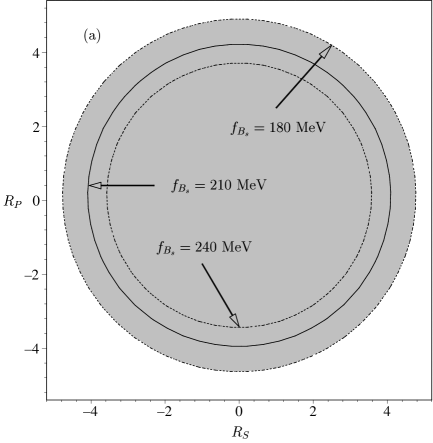
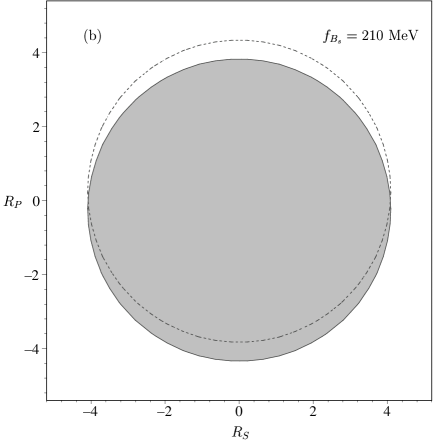
FIG. 3.: Constraints on the coefficients $R_{S}$ and $R_{P}$ as determined from the upper limit on ${\mathcal{B}}\,(\bar{B}_{s}\to\mu^{+}\mu^{-})$. (a) For $R_{10}=1$ and $f_{B_{s}}=210\pm 30\ {\text{MeV}}$. The dark region indicates the allowed region. (b) For the central value $f_{B_{s}}=210\ {\text{MeV}}$ and two choices of $R_{10}$: $-2$ (solid line) and $2$ (dashed line), as described in the text.

2 Branching ratio and FB asymmetry in $\bar{B}\to K\mu^{+}\mu^{-}$

We now assess the implications of scalar and pseudoscalar interactions for the branching ratio and forward-backward asymmetry. For the paper to be self-contained, we also provide the analytic expression for the $\bar{B}\to K^{*}\mu^{+}\mu^{-}$ branching fraction. If we keep in mind that the Wilson coefficients are real, we obtain

$${\mathcal{B}}\,(\bar{B}\to K\mu^{+}\mu^{-}) = [0.042+2.846R_{10}^{2}+2.730R_{9}^{2}+0.043R_{7}^{2}+0.181R_{S}^{2}+0.182R_{P}^{2}$$ (77)

$$- 0.132R_{P}R_{10}-0.686R_{7}R_{9}+0.522R_{9}-0.065R_{7}]\times 10^{-7},$$ (78)

$${\mathcal{B}}\,(\bar{B}\to K^{*}\mu^{+}\mu^{-}) = [0.015+0.922R_{10}^{2}+0.890R_{9}^{2}+0.212R_{7}^{2}+0.014R_{S}^{2}+0.014R_{P}^{2}$$ (79)

$$- 0.015R_{P}R_{10}-0.469R_{7}R_{9}+0.177R_{9}-0.046R_{7}]\times 10^{-6},$$ (80)

where the $R$’s are defined in Eq. (76). We note that the limits on $R_{S}$ and $R_{P}$ from the upper bound on ${\mathcal{B}}\,(\bar{B}\to K\mu^{+}\mu^{-})$ [Eq. (44)] are numerically less stringent than those derived previously from $\bar{B}_{s}\to\mu^{+}\mu^{-}$. Consequently, $|R_{S,P}|\simeq 4$ is essentially the largest value that is possible. Some representative results for the branching ratios of $\bar{B}_{s}\to\mu^{+}\mu^{-}$ and $\bar{B}\to K^{(*)}\mu^{+}\mu^{-}$ are summarized in Table I.

TABLE I.: Branching ratios of the decays $\bar{B}_{s}\to\mu^{+}\mu^{-}$ and $\bar{B}\to K^{(*)}\mu^{+}\mu^{-}$ for the choice $(R_{7},R_{9},R_{10})=(-1.2,1.1,0.8)$ together with the present experimental upper limits (see Sec. IV).

$(R_{S},R_{P})$	${\mathcal{B}}\,(\bar{B}_{s}\to\mu^{+}\mu^{-})$	${\mathcal{B}}\,(\bar{B}\to K\mu^{+}\mu^{-})$	${\mathcal{B}}\,(\bar{B}\to K^{*}\mu^{+}\mu^{-})$
$(0,0)$	$1.8\times 10^{-9}$	$6.8\times 10^{-7}$	$2.8\times 10^{-6}$
$(2,2)$	$1.1\times 10^{-6}$	$8.0\times 10^{-7}$	$2.8\times 10^{-6}$
$(3,-2)$	$2.1\times 10^{-6}$	$9.3\times 10^{-7}$	$2.8\times 10^{-6}$
$(-4,0)$	$2.5\times 10^{-6}$	$9.7\times 10^{-7}$	$2.8\times 10^{-6}$
Exptl limits	$<2.6\times 10^{-6}\ ({95\%\ \mathrm{C.L.}})$	$<5.2\times 10^{-6}\ ({90\%\ \mathrm{C.L.}})$	$<4.0\times 10^{-6}\ ({90\%\ \mathrm{C.L.}})$

As can be seen, the branching ratio of $\bar{B}\to K^{*}\mu^{+}\mu^{-}$ decay is essentially unaffected by the presence of Higgs-mediated interactions since the contributions of $R_{S,P}$ in Eq. (79) are suppressed compared to those of $R_{9,10}$. Furthermore, it is important to emphasize that large effects of scalar and pseudoscalar interactions on the $\bar{B}\to K\mu^{+}\mu^{-}$ decay rate are already excluded by the upper limit on the $\bar{B}_{s}\to\mu^{+}\mu^{-}$ branching fraction. (This constraint has not been taken into account in the analysis of Ref. [32].) As for the asymmetry, our main interest is in the average FB asymmetry, which can be obtained from the expression in Eq. (32) by integrating numerator and denominator separately over the dilepton invariant mass, leading to

$$\left\langle A_{\text{FB}}\right\rangle=R_{S}(0.512+5.424R_{9}-0.681R_{7})\Bigg{(}\frac{10^{-9}}{{\mathcal{B}}\,}\Bigg{)}.$$ (81)

To gain a maximum FB asymmetry, we fix $R_{S}=-4$ and $R_{P}=0$ allowed by current experimental data on ${\mathcal{B}}\,(\bar{B}_{s}\to\mu^{+}\mu^{-})$, together with the SM value of $R_{7}=1$. Referring to Fig. 4,

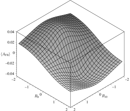
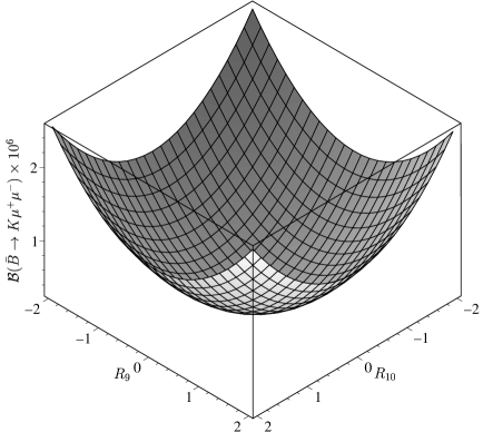
FIG. 4.: The average FB asymmetry in $\bar{B}\to K\mu^{+}\mu^{-}$ as a function of $(R_{9},R_{10})$ for $R_{S}=-4$, $R_{P}=0$, and $R_{7}=1$ consistent with the upper limit on ${\mathcal{B}}\,(\bar{B}_{s}\to\mu^{+}\mu^{-})$. Also shown is the corresponding branching ratio of $\bar{B}\to K\mu^{+}\mu^{-}$ (see the text for details).

it is evident that the average FB asymmetry in $\bar{B}\to K\mu^{+}\mu^{-}$ decay amounts to $\pm 4\%$ at most, the actual value depending on $R_{9}$ and $R_{10}$. We emphasize that some of the values of $(R_{9},R_{10})$, while respecting the upper bound on ${\mathcal{B}}\,(\bar{B}\to K\mu^{+}\mu^{-})$, are not compatible with the experimental constraint on the $\bar{B}\to K^{*}\mu^{+}\mu^{-}$ branching fraction. This is illustrated in Fig. 5, where we show the allowed range of $R_{9,10}$.

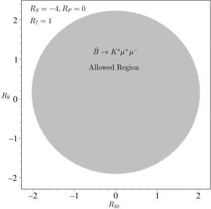
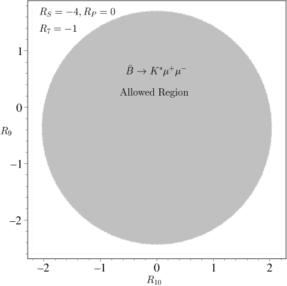
FIG. 5.: Allowed ranges of $R_{9}$ and $R_{10}$ as determined from the upper limit on ${\mathcal{B}}\,(\bar{B}\to K^{*}\mu^{+}\mu^{-})$ for $R_{S}=-4$, $R_{P}=0$, and $R_{7}=\pm 1$. Note that the values of $R_{S,P}$ are consistent with experimental data on $\bar{B}_{s}\to\mu^{+}\mu^{-}$.

Table II contains our predictions for the maximum average FB asymmetry and the branching ratios of $\bar{B}\to K^{(*)}\mu^{+}\mu^{-}$ for certain choices of parameters.

TABLE II.: Maximum values of the average FB asymmetry in $\bar{B}\to K\mu^{+}\mu^{-}$ decay together with the branching ratios of $\bar{B}\to K^{(*)}\mu^{+}\mu^{-}$ for different choices of $(R_{7},R_{9},R_{10})$. We have chosen $(R_{S},R_{P})=(-4,0)$, resulting in ${\mathcal{B}}\,(\bar{B}_{s}\to\mu^{+}\mu^{-})\simeq 2.5\times 10^{-6}$, which is close to the present upper bound of $2.6\times 10^{-6}$. Also listed are the ${90\%\ \mathrm{C.L.}}$ upper limits as discussed in Sec. IV.

$(R_{7},R_{9},R_{10})$	$\left\langle A_{\text{FB}}\right\rangle$	${\mathcal{B}}\,(\bar{B}\to K\mu^{+}\mu^{-})$	${\mathcal{B}}\,(\bar{B}\to K^{*}\mu^{+}\mu^{-})$
$(1,1.9,1)$	$-2.6\%$	$1.5\times 10^{-6}$	$3.8\times 10^{-6}$
$(-1,1.2,1.3)$	$-2.3\%$	$1.3\times 10^{-6}$	$3.9\times 10^{-6}$
$(1,1,1)$	$-2.5\%$	$8.3\times 10^{-7}$	$1.7\times 10^{-6}$
$(1,-1,0)$	$+3.8\%$	$5.8\times 10^{-7}$	$1.4\times 10^{-6}$
$(1,1,0)$	$-3.8\%$	$5.5\times 10^{-7}$	$7.8\times 10^{-7}$
$(-1.2,1.1,0.8)$	$-3.0\%$	$9.7\times 10^{-7}$	$2.8\times 10^{-6}$
Exptl limits	$-$	$<5.2\times 10^{-6}$	$<4.0\times 10^{-6}$

Note that the measurement of a nominal asymmetry of $4\%$ (at $3\sigma$ level), which is accompanied by a branching fraction of $\sim 6\times 10^{-7}$, will necessitate at least $\sim 10^{10}$ $B$ mesons and could conceivably be measured in forthcoming experiments at the CERN Large Hadron Collider (LHC) and the Tevatron. We conclude that the predicted FB asymmetry due to scalar interactions, though larger than in the SM, may possibly be too small to be seen experimentally. Nevertheless, the FB asymmetry does provide a very useful laboratory for studying possible extensions of the SM.

B Constraints on new physics with minimal flavour violation

It is clear from the previous analysis that the upper bound on the $\bar{B}_{s}\to\mu^{+}\mu^{-}$ branching fraction gives the strongest constraints on the scalar and pseudoscalar couplings, $c_{S,P}$, which in turn can be used to restrict the parameter space of models outside the SM.

1 Two-Higgs-doublet model

Using the constraints of the preceding sections, together with the results for the Wilson coefficients of scalar and pseudoscalar operators [Eq. (62)], we obtain exclusions in the $(m_{H^{\pm}},R_{S})$ plane, shown in Fig. 6.

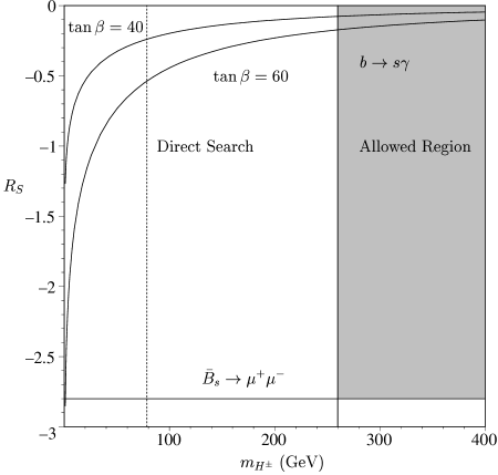
FIG. 6.: $R_{S}$ vs the charged Higgs-boson mass in the 2HDM for large values of $\tan\beta$, taking into account the constraint from $\bar{B}_{s}\to\mu^{+}\mu^{-}$ decay. We exhibit the cases of $\tan\beta=40$ and $\tan\beta=60$, and also show, for comparison, lower limits on the Higgs-boson mass obtained by direct searches at the CERN $e^{+}e^{-}$ collider LEP [33] (vertical line at $m_{H^{\pm}}=78.5\ {\text{GeV}}$) and by the measured $b\to s\gamma$ rate, using the leading-order result for the branching fraction.

The observation to be noted here concerns the measured $b\to s\gamma$ branching fraction, which gives the strongest constraint on the Higgs-boson mass, thereby placing an upper bound on $|R_{S}|$ of $0.17$. As a consequence, the FB asymmetry due to non-standard scalar interactions turns out to be exceedingly small, typically of the order of $O(10^{-3})$. It should also be remarked that the lower bound on the charged Higgs-boson mass, $m_{H^{\pm}}\approx 260\ {\text{GeV}}$, obtained from the measured inclusive $b\to s\gamma$ fraction in the context of the type-II 2HDM, does not directly apply to supersymmetric extensions of the SM since the chargino amplitude may interfere destructively with the charged Higgs- and $W$-boson contributions. Given a charged Higgs-boson mass of $m_{H^{\pm}}=260\ {\text{GeV}}$, the branching ratio of $\bar{B}_{s}\to\mu^{+}\mu^{-}$ amounts to $(1.4$–$4.8)\times 10^{-9}$ for $40\leqslant\tan\beta\leqslant 60$, which should be compared with the SM result of $(3.1\pm 1.4)\times 10^{-9}$ [Eq. (42)]. The average FB asymmetry is estimated to lie in the interval $-0.7\times 10^{-3}\leqslant\left\langle A_{\text{FB}}\right\rangle\leqslant-1.6\times 10^{-3}$, which is much too small to be detected. For the decays $\bar{B}\to K\mu^{+}\mu^{-}$ and $\bar{B}\to K^{*}\mu^{+}\mu^{-}$, we predict branching ratios of $5.2\times 10^{-7}$ and $1.7\times 10^{-6}$ respectively (to be compared with the SM expectations of about $6\times 10^{-7}$ and $2\times 10^{-6}$). Note that these decays are largely unaffected by the charged Higgs-boson contributions to $R_{9},R_{10}$, which are proportional to $\cot^{2}\beta$, and hence small in the large $\tan\beta$ regime.

Our conclusion is therefore that current experimental data on various rare $B$ decays – apart from $b\to s\gamma$ – do not provide any constraints on the parameter space in two-Higgs-doublet models of class II. Moreover, the predictions for the branching ratios of the $B$ decay modes under study are comparable to those of the SM. We next turn to the SUSY scenario.

2 SUSY with minimal flavour violation

As mentioned earlier, we do not consider any $\mathrm{CP}$-violating effects, and consequently the SUSY parameters and mixing matrices discussed in the previous section can be taken to be real. We further assume the sneutrinos to be degenerate in mass so that $R_{\tilde{\nu}}$, which enters the expression in Eq. (64), reduces to the unit matrix.

For the sake of illustration, we perform the numerical analysis for a light stop $\tilde{t}_{1}$, with large mixing $\theta_{\tilde{t}}$, and charginos with large Higgsino components. We impose the lower bounds on the SUSY particle masses as compiled by the Particle Data Group [21]. In the case of a light scalar top quark, there are additional constraints coming from electroweak measurements such as the $\rho$ parameter [34]. As for the constraint from $b\to s\gamma$, it is well known that within supersymmetry there are chargino-stop contributions, in addition to charged Higgs boson and $W$ boson loop contributions, which can significantly affect the $b\to s\gamma$ decay rate in the large $\tan\beta$ region, thereby leading to constraints on the parameter space. This is due to the fact that at large $\tan\beta$, the chargino loop contributions grow linearly with $\tan\beta$ (see, e.g., Ref. [36]). Thus, in order to satisfy the $b\to s\gamma$ bounds, we must require that chargino and charged Higgs- and $W$-boson contributions interfere destructively, so that significant cancellations can occur. Note that in this case the sign of the Wilson coefficient $c_{7}^{\text{eff}}$ is opposite to the SM one.

Using the expressions for the scalar and pseudoscalar Wilson coefficients, Eqs. (62), (64)–(69), we obtain the allowed $(m_{H^{\pm}},m_{\tilde{\chi}^{\pm}_{1}})$ region displayed in Fig. 7 for $m_{\tilde{t}_{1}}=120\ {\text{GeV}}$ and $\theta_{\tilde{t}}\approx-45^{\circ}$. As can be seen, the present upper limit on ${\mathcal{B}}\,(\bar{B}_{s}\to\mu^{+}\mu^{-})$ already excludes a significant portion of the SUSY parameter space with charged Higgs-boson and chargino masses. Remembering that the SM prediction for the branching ratio is of order $O(10^{-9})$, it is clear that within the context of SUSY, the $\bar{B}_{s}\to\mu^{+}\mu^{-}$ branching fraction can be increased by several orders of magnitude, due to the $\tan^{3}\beta$ enhancement of the counterterm diagrams [Eq. (69)].

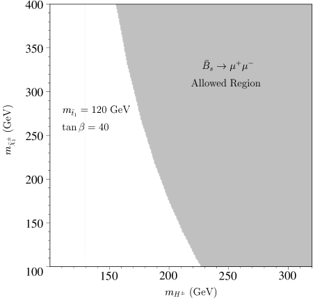
FIG. 7.: Allowed region in the $(m_{H^{\pm}},m_{\tilde{\chi}^{\pm}_{1}})$ plane derived from the upper bound on ${\mathcal{B}}\,(\bar{B}_{s}\to\mu^{+}\mu^{-}$) for a light stop with $m_{\tilde{t}_{1}}=120\ {\text{GeV}}$ and maximal mixing, $\theta_{\tilde{t}}\approx-45^{\circ}$.

Given a chargino mass of $m_{\tilde{\chi}^{\pm}_{1}}=297\ {\text{GeV}}$, the SUSY prediction for $R_{S,P}$, consistent with the upper bound on ${\mathcal{B}}\,(\bar{B}_{s}\to\mu^{+}\mu^{-})$, is shown in Fig. 8(a), as a function of the charged Higgs-boson mass. From this we infer that $R_{S,P}$ are constrained to lie in the range $-3\lesssim R_{S,P}\lesssim 3$, leading to an average FB asymmetry of less than $2\%$. Figure 8(b) displays the dependency of the $\bar{B}_{s}\to\mu^{+}\mu^{-}$ branching ratio on the charged Higgs-boson mass for $m_{\tilde{\chi}^{\pm}_{1}}=297\ {\text{GeV}}$.

FIG. 8.: SUSY predictions for (a) $R_{S,P}$ and (b) the branching ratio of $\bar{B}_{s}\to\mu^{+}\mu^{-}$ at large $\tan\beta$, as a function of the charged Higgs-boson mass, with $m_{\tilde{t}_{1}}=120\ {\text{GeV}}$, $\theta_{\tilde{t}}\approx-45^{\circ}$, and $m_{\tilde{\chi}^{\pm}_{1}}=297\ {\text{GeV}}$. We note that this choice of parameters satisfies all experimental bounds.

Thus, the measurement of the $\bar{B}_{s}\to\mu^{+}\mu^{-}$ branching fraction, together with the $b\to s\gamma$ bounds, provides a useful tool for constraining supersymmetric extensions of the SM. Finally, for the above parameter space point and $m_{H^{\pm}}=170\ {\text{GeV}}$, we obtain ${\mathcal{B}}\,(\bar{B}\to K\mu^{+}\mu^{-})=1.0\times 10^{-6}$ and ${\mathcal{B}}\,(\bar{B}\to K^{*}\mu^{+}\mu^{-})=2.6\times 10^{-6}$ to be compared with the present upper limits of $5.2\times 10^{-6}$ and $4.0\times 10^{-6}$.

VII Summary and conclusions

We have carried out a study of exclusive $B$ decays governed by the $b\to sl^{+}l^{-}$ transition in extensions of the SM with minimal flavour violation and new scalar and pseudoscalar interactions, focusing on the dimuon final state, and taking account of existing experimental data on $b\to s\gamma$ as well as the upper limits on $\bar{B}_{s}\to\mu^{+}\mu^{-}$ and $\bar{B}\to K^{(*)}\mu^{+}\mu^{-}$ decays. We have restricted the discussion to the interesting case of large $\tan\beta$, which may compensate for the inevitable suppression of scalar and pseudoscalar couplings by the lepton mass of $e$ or $\mu$. Our main findings can be summarized as follows.

We have presented in a model-independent manner expressions for the $\bar{B}_{s}\to l^{+}l^{-}$ branching fraction and the differential decay spectrum of $\bar{B}\to Kl^{+}l^{-}$, together with the corresponding FB asymmetry, which is extremely tiny within the SM. In particular, we find that scalar and pseudoscalar interactions can, in principle, lead to striking effects in the decay distribution of $\bar{B}\to K\mu^{+}\mu^{-}$, while the branching ratio of $\bar{B}\to K^{*}\mu^{+}\mu^{-}$ is essentially unaffected by the Higgs-boson contributions. We have demonstrated that once the constraint from $\bar{B}_{s}\to\mu^{+}\mu^{-}$ is taken into account, the effects of scalar and pseudoscalar couplings on the decay $\bar{B}\to K\mu^{+}\mu^{-}$ are much smaller. In view of the inherent uncertainty of the predictions for exclusive $B$ decays due to the form factors, it seems extremely unlikely that a measurement of the decay spectrum alone can provide a clue to new physics with scalar and pseudoscalar interactions. We have also investigated the FB asymmetry of $\mu^{-}$ in $\bar{B}\to K\mu^{+}\mu^{-}$ decay, which turns out to be at the level of a few per cent. Our analysis suggests that the observation of a nominal FB asymmetry of, say, $4\%$, together with a branching ratio of about $6\times 10^{-7}$, will be challenging but might be feasible at the LHC and the Tevatron. As more precise data on the $\bar{B}_{s}\to\mu^{+}\mu^{-}$ branching ratio are available, more stringent upper limits will be placed on the FB asymmetry due to scalar interactions. The essential conclusion of our model-independent analysis is that current experimental data on $\bar{B}_{s}\to\mu^{+}\mu^{-}$ decay already exclude large values of the Wilson coefficients $c_{S}$ and $c_{P}$ of scalar and pseudoscalar operators, so that striking effects are not likely to show up in the decay spectrum of $\bar{B}\to K\mu^{+}\mu^{-}$ and the corresponding FB asymmetry of the muon. Even so, the FB asymmetry provides an independent window to physics beyond the SM, especially to models with an extended Higgs sector, and its observation would be an unambiguous signal of new physics.

In extensions of the SM with minimal flavour violation, we have calculated the Higgs-boson contributions to the Wilson coefficients of scalar and pseudoscalar operators, and investigated how the new-physics parameters are constrained by existing experimental data on rare $B$ decays. Within the type-II 2HDM framework, where the Higgs sector corresponds to the one of the MSSM, we found no appreciable FB asymmetry or any large deviation from the SM prediction for the $\bar{B}\to K^{(*)}\mu^{+}\mu^{-}$ branching fractions. As for the decay $\bar{B}_{s}\to\mu^{+}\mu^{-}$, the branching ratio turns out to be in the range $(1.4$–$4.8)\times 10^{-9}$ for $40\leqslant\tan\beta\leqslant 60$ and $m_{H^{\pm}}=260\ {\text{GeV}}$, which is within the errors of the SM prediction of $(3.1\pm 1.4)\times 10^{-9}$. Ultimately, the smallness of the new-physics contributions is caused by the mass of the charged Higgs boson, which is strongly constrained by the measured $b\to s\gamma$ branching fraction ($m_{H^{\pm}}\gtrsim 260\ {\text{GeV}}$). We therefore conclude that within the type-II 2HDM there are no sizable new-physics effects on the $B$ decay modes described above, apart from $b\to s\gamma$. By contrast, within SUSY, the effects of chargino and neutral Higgs-boson contributions on the $\bar{B}_{s}\to\mu^{+}\mu^{-}$ branching fraction can be enormous while satisfying the $b\to s\gamma$ bounds. We have considered a SUSY scenario with a scalar top quark with large mixing and a mass much lighter than the scalar partners of the light quarks. We find that for a given set of parameters obeying the $b\to s\gamma$ constraint, the upper limit on ${\mathcal{B}}\,(\bar{B}_{s}\to\mu^{+}\mu^{-})$ severely constrains the masses of charginos and charged Higgs bosons. As a typical result, the lower bound $m_{H^{\pm}}\gtrsim 170\ {\text{GeV}}$ has been derived for $m_{\tilde{\chi}^{\pm}_{1}}=297\ {\text{GeV}}$, $m_{\tilde{t}_{1}}=120\ {\text{GeV}}$, and $\theta_{\tilde{t}}\approx-45^{\circ}$. The remaining observables are estimated to be $\left\langle A_{\text{FB}}\right\rangle=1.8\%$ and ${\mathcal{B}}\,(\bar{B}\to K^{(*)}\mu^{+}\mu^{-})=1.0\ (2.6)\times 10^{-6}$ (for $m_{H^{\pm}}=170\ {\text{GeV}}$), the latter being close to the present upper limits. Clearly, the analysis of the decay $\bar{B}_{s}\to\mu^{+}\mu^{-}$ is complementary to the study of $\bar{B}\to K^{(*)}\mu^{+}\mu^{-}$ and $b\to s\gamma$ decays, which leads to constraints on the remaining short-distance coefficients, $c_{7}^{\text{eff}},c_{9}^{\text{eff}}$, and $c_{10}$. A combined analysis of these decay modes, therefore, provides a powerful tool to constrain physics transcending the SM.

Note added in proof. As this paper was readied for publication, we received a paper by Huang et al. [37] that corrects the result presented for the 2HDM in Ref. [10]. The result of Ref. [37] coincides with that of the present paper [Eq. (75)].

A Useful functions

1 The one-loop function $Y(s)$

The function $Y(s)$ appearing in Eq. (38) is given by [14]

$$Y(s) = g(m_{c},s)(3c_{1}+c_{2}+3c_{3}+c_{4}+3c_{5}+c_{6})-\frac{1}{2}g(0,s)(c_{3}+3c_{4})$$ (A1)

$$- \frac{1}{2}g(m_{b},s)(4c_{3}+4c_{4}+3c_{5}+c_{6})+\frac{2}{9}(3c_{3}+c_{4}+3c_{5}+c_{6}),$$ (A2)

where (at $\mu_{b}=m_{b}^{\text{pole}}$)

$$g(m_{i},s)=-\frac{8}{9}\ln(m_{i}/m_{b}^{\text{pole}})+\frac{8}{27}+\frac{4}{9}y_{i}-\frac{2}{9}(2+y_{i})\sqrt{|1-y_{i}|}$$ (A4)

$$\times\left\{\Theta(1-y_{i})\left[\ln\left(\frac{1+\sqrt{1-y_{i}}}{1-\sqrt{1-y_{i}}}\right)-i\pi\right]+\Theta(y_{i}-1)2\arctan\frac{1}{\sqrt{y_{i}-1}}\right\},$$

with $y_{i}=4m_{i}^{2}/s$, and

$$c_{1}=-0.249,\ c_{2}=1.107,\ c_{3}=0.011,\ c_{4}=-0.025,\ c_{5}=0.007,\ c_{6}=-0.031.$$ (A5)

In Eq. (A1), we have omitted the one-gluon correction to the matrix element of the operator ${\mathcal{O}}_{9}$, which can be regarded as a contribution to the form factors.

2 Auxiliary functions

$$B(x,y)=\frac{y}{x-y}\left[\frac{\ln y}{y-1}-\frac{\ln x}{x-1}\right],$$ (A6)

$$C(x,y)=\frac{y}{x-y}\left[\frac{x\ln x}{x-1}-\frac{y\ln y}{y-1}\right],$$ (A7)

$$D_{1}(x,y,z)=\frac{x\ln x}{(1-x)(x-y)(x-z)}+(x\leftrightarrow y)+(x\leftrightarrow z),$$ (A8)

$$D_{2}(x,y)=\frac{x\ln x}{(1-x)(x-y)}+(x\leftrightarrow y),$$ (A9)

$$D_{3}(x)=\frac{x\ln x}{1-x}.$$ (A10)

B SUSY mass and mixing matrices

For the reader’s convenience and to fix our notation, we give here the relevant mass and mixing matrices in the context of SUSY, for which we adopt the conventions of Ref. [29].

1 Chargino mass matrix

Neglecting new $\mathrm{CP}$-violating phases, the chargino mass matrix is given by

$$M_{\tilde{\chi}^{\pm}}=\left(\begin{array}[]{cc}M_{2}&\sqrt{2}M_{W}\sin\beta\\ \sqrt{2}M_{W}\cos\beta&\mu\end{array}\right),$$ (B1)

where $M_{2}$ and $\mu$ are the $W$-ino and Higgsino mass parameters respectively. This matrix can be cast in diagonal form by means of a biorthogonal transformation

$$UM_{\tilde{\chi}^{\pm}}V^{\text{T}}={\mathrm{diag}}(m_{\tilde{\chi}^{\pm}_{1}},m_{\tilde{\chi}^{\pm}_{2}}),$$ (B2)

$m_{\tilde{\chi}^{\pm}_{1,2}}$ being the chargino masses with $m^{2}_{\tilde{\chi}^{\pm}_{1}}<m^{2}_{\tilde{\chi}^{\pm}_{2}}$. The orthogonal matrices $U$, $V$ read

$$U=\left(\begin{array}[]{cc}\cos\theta_{U}&\sin\theta_{U}\\ -\sin\theta_{U}&\cos\theta_{U}\end{array}\right),\quad V=\left(\begin{array}[]{cc}\cos\theta_{V}&\sin\theta_{V}\\ -\sin\theta_{V}&\cos\theta_{V}\end{array}\right),$$ (B3)

with the mixing angles

$$\sin 2\theta_{U,V}=\frac{2M_{W}\big{[}M_{2}^{2}+\mu^{2}\pm(M_{2}^{2}-\mu^{2})\cos 2\beta+2\mu M_{2}\sin 2\beta]^{1/2}}{m^{2}_{\tilde{\chi}^{\pm}_{1}}-m^{2}_{\tilde{\chi}^{\pm}_{2}}},$$ (B4)

$$\cos 2\theta_{U,V}=\frac{M_{2}^{2}-\mu^{2}\mp 2M_{W}^{2}\cos 2\beta}{m^{2}_{\tilde{\chi}^{\pm}_{1}}-m^{2}_{\tilde{\chi}^{\pm}_{2}}}.$$ (B5)

2 Scalar top mass matrix

In the $(\tilde{U}_{L},\tilde{U}_{R})$ basis, the $6\times 6$ up-type squark mass-squared matrix is given by

$$M^{2}_{\tilde{U}}=\left(\begin{array}[]{cc}M^{2}_{\tilde{U}_{LL}}&M^{2}_{\tilde{U}_{LR}}\\ M^{2}_{\tilde{U}_{LR}}&M^{2}_{\tilde{U}_{RR}}\end{array}\right),$$ (B6)

which can be diagonalized by an orthogonal matrix $R_{\tilde{U}}$ such that

$$R_{\tilde{U}}M_{\tilde{U}}^{2}R_{\tilde{U}}^{\text{T}}={\mathrm{diag}}(m_{\tilde{u}_{1}}^{2},m_{\tilde{u}_{2}}^{2},\dots,m_{\tilde{u}_{6}}^{2}).$$ (B7)

Since we ignore flavour-mixing effects among squarks, the matrix in Eq. (B6) decomposes into a series of $2\times 2$ matrices. Working in the so-called super-CKM basis [38], in which the quark mass matrices are diagonal, and squarks as well as quarks are rotated simultaneously, the LR terms in Eq. (B6) are proportional to $m_{q}$, $q=u,c,t$. Thus, large mixing can occur only in the scalar top quark sector, leading to a mass eigenstate $m_{\tilde{t}_{1}}$ possibly much lighter than the remaining squarks.

Defining the $6\times 3$ matrices

$$(\Gamma^{U_{L}})_{ai}=(R_{\tilde{U}})_{ai},\quad(\Gamma^{U_{R}})_{ai}=(R_{\tilde{U}})_{a,i+3},$$ (B8)

we obtain

$$(\Gamma^{U_{L}})^{\text{T}}=\left(\begin{array}[]{cccccc}1&0&0&0&0&0\\ 0&1&0&0&0&0\\ 0&0&\cos\theta_{\tilde{t}}&0&0&-\sin\theta_{\tilde{t}}\end{array}\right),\quad(\Gamma^{U_{R}})^{\text{T}}=\left(\begin{array}[]{cccccc}0&0&0&1&0&0\\ 0&0&0&0&1&0\\ 0&0&\sin\theta_{\tilde{t}}&0&0&\cos\theta_{\tilde{t}}\end{array}\right),$$ (B9)

with the mixing angle $(-\pi/2\leqslant\theta_{\tilde{t}}\leqslant\pi/2$)

$$\sin 2\theta_{\tilde{t}}=\frac{2m_{t}(A_{t}-\mu\cot\beta)}{m_{\tilde{t}_{1}}^{2}-m_{\tilde{t}_{2}}^{2}},\quad\cos 2\theta_{\tilde{t}}=\frac{(m_{\tilde{t}_{L}}^{2}-m_{\tilde{t}_{R}}^{2})+\frac{1}{6}M_{Z}^{2}\cos 2\beta(3-8\sin^{2}\theta_{W})}{m_{\tilde{t}_{1}}^{2}-m_{\tilde{t}_{2}}^{2}}.$$ (B10)

Here $A_{t}$ is the trilinear coupling, $m_{\tilde{t}_{L,R}}$ are the soft SUSY-breaking scalar masses, and $m_{\tilde{t}_{1,2}}$ denote the stop masses with $m^{2}_{\tilde{t}_{1}}<m^{2}_{\tilde{t}_{2}}$.

3 Sneutrino mixing matrix

The $3\times 3$ mixing matrix $R_{\tilde{\nu}}$ appearing in Eq. (64) is defined via

$$R_{\tilde{\nu}}M_{\tilde{\nu}}^{2}R_{\tilde{\nu}}^{\text{T}}={\mathrm{diag}}(m_{\tilde{\nu}_{1}}^{2},m_{\tilde{\nu}_{2}}^{2},m_{\tilde{\nu}_{3}}^{2}),$$ (B11)

where $M_{\tilde{\nu}}^{2}$ is the sneutrino mass-squared matrix (see, e.g., Refs. [39, 38]).

REFERENCES

• [1] H. P. Nilles, Phys. Rep. 110, 1 (1984); H. E. Haber and G. L. Kane, ibid. 117, 75 (1985); J. F. Gunion and H. E. Haber, Nucl. Phys. B272, 1 (1986); B402, 567(E) (1993).
• [2] J. F. Gunion, H. E. Haber, G. L. Kane, and S. Dawson, The Higgs Hunter’s Guide (Addison-Wesley, Reading, MA, 1990); hep-ph/9302272.
• [3] G. Buchalla and A. J. Buras, Nucl. Phys. B400, 225 (1993); B548, 309 (1999).
• [4] X. G. He, T. D. Nguyen, and R. R. Volkas, Phys. Rev. D 38, 814 (1988); J. L. Hewett, S. Nandi, and T. G. Rizzo, ibid. 39, 250 (1989); M. J. Savage, Phys. Lett. B 266, 135 (1991); Y. Grossman, Nucl. Phys. B426, 355 (1994).
• [5] W. Skiba and J. Kalinowski, Nucl. Phys. B404, 3 (1993), and references therein.
• [6] Y. Grossman, Z. Ligeti, and E. Nardi, Phys. Rev. D 55, 2768 (1997).
• [7] Y.-B. Dai, C.-S. Huang, and H.-W. Huang, Phys. Lett. B 390, 257 (1997); C.-S. Huang and Q.-S. Yan, Phys. Lett. B 442, 209 (1998); C.-S. Huang, W. Liao, and Q.-S. Yan, Phys. Rev. D 59, 011701 (1999); S. R. Choudhury and N. Gaur, Phys. Lett. B 451, 86 (1999); K. S. Babu and C. Kolda, Phys. Rev. Lett. 84, 228 (2000).
• [8] D. Guetta and E. Nardi, Phys. Rev. D 58, 012001 (1998).
• [9] H. E. Logan and U. Nierste, Nucl. Phys. B586, 39 (2000).
• [10] C.-S. Huang, W. Liao, Q.-S. Yan, and S.-H. Zhu, Phys. Rev. D 63, 114021 (2001).
• [11] P. H. Chankowski and Ł. Sławianowska, Phys. Rev. D 63, 054012 (2001).
• [12] CDF Collaboration, F. Abe et al., Phys. Rev. D 57, 3811 (1998).
• [13] CDF Collaboration, T. Affolder et al., Phys. Rev. Lett. 83, 3378 (1999).
• [14] A. J. Buras and M. Münz, Phys. Rev. D 52, 186 (1995); M. Misiak, Nucl. Phys. B393, 23 (1993); B439, 461(E) (1995).
• [15] G. Buchalla, A. J. Buras, and M. E. Lautenbacher, Rev. Mod. Phys. 68, 1125 (1996).
• [16] S. Fukae, C. S. Kim, T. Morozumi, and T. Yoshikawa, Phys. Rev. D 59, 074013 (1999).
• [17] M. Wirbel, B. Stech, and M. Bauer, Z. Phys. C 29, 637 (1985).
• [18] A. Ali, P. Ball, L. T. Handoko, and G. Hiller, Phys. Rev. D 61, 074024 (2000).
• [19] D. Melikhov and B. Stech, Phys. Rev. D 62, 014006 (2000).
• [20] For recent reviews, see C. T. Sachrajda, Nucl. Instrum. Methods Phys. Res. A462, 23 (2001); J. Flynn and C.-J. D. Lin, J. Phys. G 27, 1245 (2001); L. Lellouch and C.-J. D. Lin, Phys. Rev. D (to be published), hep-ph/0011086.
• [21] Particle Data Group, D. E. Groom et al., Eur. Phys. J. C 15, 1 (2000).
• [22] A. Ali, T. Mannel, and T. Morozumi, Phys. Lett. B 273, 505 (1991); F. Krüger and L. M. Sehgal, ibid. 380, 199 (1996); Z. Ligeti, I. W. Stewart, and M. B. Wise, ibid. 420, 359 (1998).
• [23] ALEPH Collaboration, R. Barate et al., Phys. Lett. B 429, 169 (1998); CLEO Collaboration, S. Ahmed et al., hep-ex/9908022.
• [24] A. L. Kagan and M. Neubert, Eur. Phys. J. C 7, 5 (1999).
• [25] CLEO Collaboration, T. Bergfeld et al., Phys. Rev. D 62, 091102 (2000).
• [26] For a recent review, see A. J. Buras, hep-ph/0101336, and references therein.
• [27] S. Bertolini, F. Borzumati, A. Masiero, and G. Ridolfi, Nucl. Phys. B353, 591 (1991).
• [28] P. Cho, M. Misiak, and D. Wyler, Phys. Rev. D 54, 3329 (1996); T. Goto, Y. Okada, Y. Shimizu, and M. Tanaka, ibid. 55, 4273 (1997).
• [29] F. Krüger and J. C. Romão, Phys. Rev. D 62, 034020 (2000).
• [30] J. Rosiek, Phys. Rev. D 41, 3464 (1990); hep-ph/9511250.
• [31] C. Bobeth, T. Ewerth, F. Krüger, and J. Urban (in preparation).
• [32] Q.-S. Yan, C.-S. Huang, W. Liao, and S.-H. Zhu, Phys. Rev. D 62, 094023 (2000).
• [33] LEP Higgs Working Group, http://lephiggs.web.cern.ch/LEPHIGGS/www/.
• [34] See, for example, M. Drees and K. Hagiwara, Phys. Rev. D 42, 1709 (1990); J. Erler and D. M. Pierce, Nucl. Phys. B526, 53 (1998); A. Djouadi et al., hep-ph/0002258.
• [35] H. Baer, M. Brhlik, D. Castaño, and X. Tata, Phys. Rev. D 58, 015007 (1998).
• [36] Y. Okada, Phys. Lett. B 315, 119 (1993); R. Garisto and J. N. Ng, ibid. 315, 372 (1993); N. Oshimo, Nucl. Phys. B404, 20 (1993); T. Goto and Y. Okada, Prog. Theor. Phys. 94, 407 (1995); J. L. Hewett and J. D. Wells, Phys. Rev. D 55, 5549 (1997).
• [37] C.-S. Huang, W. Liao, Q.-S. Yan, and S.-H. Zhu, Phys. Rev. D 64, 059902(E) (2001).
• [38] M. Misiak, S. Pokorski, and J. Rosiek, in Heavy Flavours II, edited by A. J. Buras and M. Lindner (World Scientific, Singapore, 1998), p. 795, hep-ph/9703442.
• [39] J. C. Romão, hep-ph/9811454.