The Color Glass Condensate and Small x
Physics: 4 Lectures.

Summary.

The Color Glass Condensate is a state of high density gluonic matter which controls the high energy limit of hadronic matter. These lectures begin with a discussion of general problems of high energy strong interactions. The infinite momentum frame description of a single hadron at very small x is developed, and this picture is applied to the description of ultrarelativistic nuclear collisions. Recent developments in the renormalization group description of the Color Glass Condensate are reviewed.

1 Lecture I: General Considerations

1.1 Introduction

QCD is the correct theory of hadronic physics. It has been tested in various experiments. For high energy short distance phenomena, perturbative QCD computations successfully confront experiment. In lattice Monte-Carlo computations, one gets a successful semi-quantitative description of hadronic spectra, and perhaps in the not too distant future one will obtain precise quantitative agreement.

At present, however, all analytic computations and all precise QCD tests are limited to a small class of problems which correspond to short distance physics, or to semi-quantitative comparisons with the results of lattice gauge theory numerical computations. For the short distance phenomena, there is some characteristic energy transfer scale $E$, and one uses asymptotic freedom,

$$\alpha_{S}(E)\rightarrow 0$$ (1)

as $E\rightarrow\infty$ For example, in Fig. 1, two hadrons collide to make a pair of jets. If the transverse momenta of the jets is large, the strong coupling strength which controls this production is evaluated at the $p_{T}$ of the jet. If $p_{T}>>\Lambda_{QCD}$, then the coupling is weak and this process can be computed in perturbation theory.

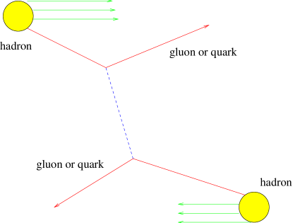
Figure 1: Hadron-hadron scattering to produce a pair of jets.

QCD has also been extensively tested in deep inelastic scattering. In Fig. 2, an electron exchanges a virtual photon with a hadronic target. If the virtual photon momentum transfer $Q$ is large, then one can use weak coupling methods.

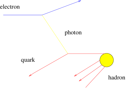
Figure 2: Deep inelastic scattering of an electron on a hadron.

One question which we might ask is whether there are non-perturbative “simple phenomena” which arise from QCD which are worthy of further effort. The questions I would ask before I would become interested in understanding such phenomena are

• Is the phenomenon simple in structure?

• Is the phenomena pervasive?

• Is it reasonably plausible that one can understand the phenomena from first principles, and compute how it would appear in nature?

I will argue that gross or typical processes in QCD, which by their very nature are pervasive, appear to follow simple patterns. The main content of this first lecture is to show some of these processes, and pose some simple questions about their nature which we do not yet understand.

My goal is to convince you that much of these average phenomena of strong interactions at extremely high energies is controlled by a new form of hadronic matter, a dense condensate of gluons. This is called the Color Glass Condensate since

• Color: The gluons are colored.

• Glass: We shall see that the fields associated with the glass evolve very slowly relative to natural time scales, and are disordered. This is like a glass which is disordered and is a liquid on long time scales but seems to be a solid on short time scales.

• Condensate: There is a very high density of massless gluons. These gluons can be packed until their phase space density is so high that interactions prevent more gluon occupation. This forces at increasingly high density the gluons to occupy higher momenta, and the coupling becomes weak. The density saturates at $dN/d^{2}p_{T}d^{2}r_{T}\sim 1/\alpha_{s}>>1$, and is a condensate.

In these lectures, I will try to explain why the above is very plausible.

1.2 Total Cross Sections at Asymptotic Energy

Computing total cross sections as $E\rightarrow\infty$ is one of the great unsolved problems of QCD. Unlike for processes which are computed in perturbation theory, it is not required that any energy transfer become large as the total collision energy $E\rightarrow\infty$. Computing a total cross section for hadronic scattering therefore appears to be intrinsically non-perturbative. In the 60’s and early 70’s, Regge theory was extensively developed in an attempt to understand the total cross section. The results of this analysis were to my mind inconclusive, and certainly can not be claimed to be a first principles understanding from QCD.

The total cross section for $pp$ and $\overline{p}p$ collisions is shown in Fig. 3.

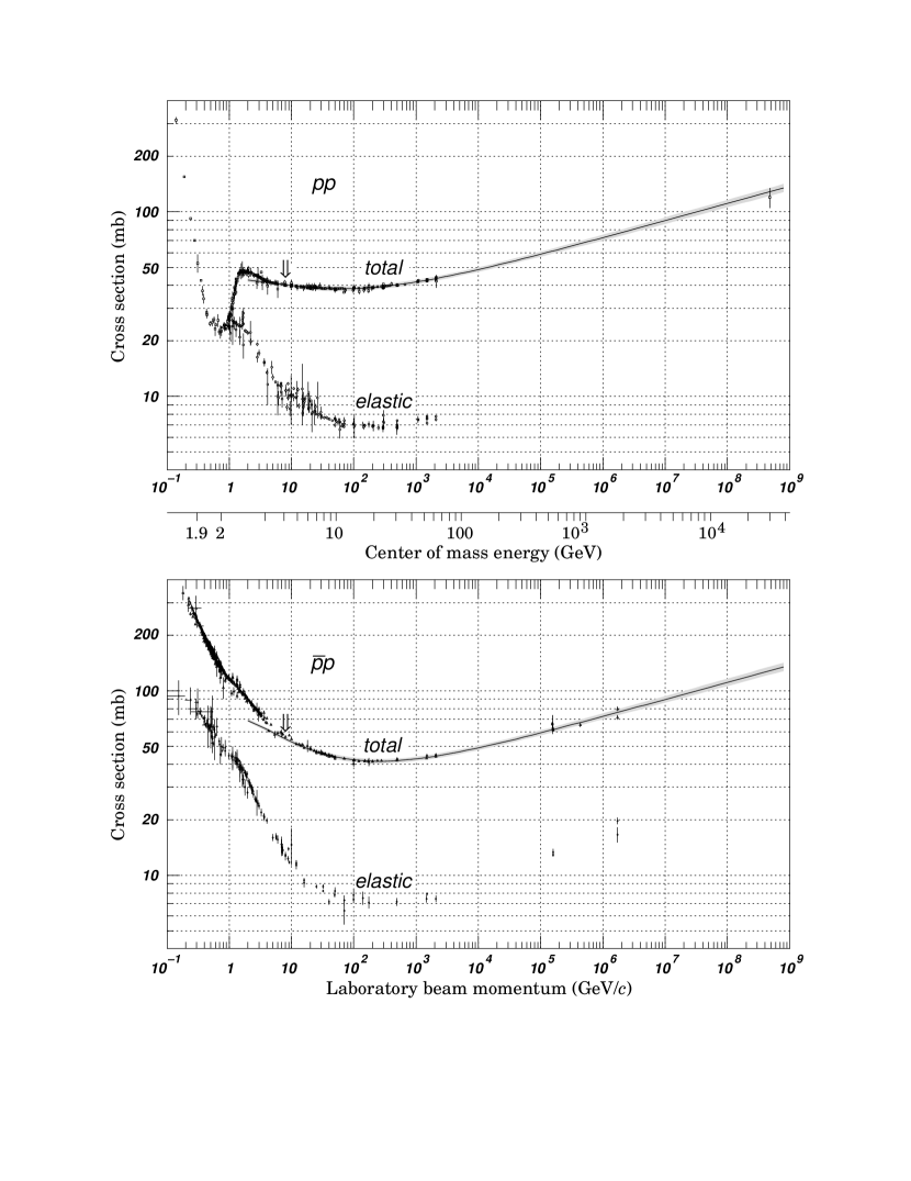
Figure 3: The cross sections for $pp$ and $p\overline{p}$ scattering.

Typically, it is assumed that the total cross section grows as $ln^{2}E$ as $E\rightarrow\infty$. This is the so called Froisart bound which corresponds to the maximal growth allowed by unitarity of the S matrix. Is this correct? Is the coefficient of $ln^{2}E$ universal for all hadronic precesses? Why is the unitarity limit saturated? Can we understand the total cross section from first principles in QCD? Is it understandable in weakly coupled QCD, or is it an intrinsically non-perturbative phenomenon?

1.3 How Are Particles Produced in High Energy Collisions?

In Fig. 4 , I plot the multiplicity of produced particles in $pp$ and in $\overline{p}p$ collisions. The last six points correspond to the $\overline{p}p$ collisions. The three upper points are the multiplicity in $p\overline{p}$ collisions, and the bottom three have the mutliplicity at zero energy subtracted. The remaining points correspond to $pp$. Notice that the $pp$ points and those for $p\overline{p}$ with zero energy multiplicity subtracted fall on the same curve. The implication is that whatever is causing the increase in multiplicity in these collisions may be from the same mechanism.

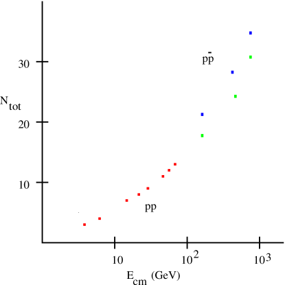
Figure 4: The total multiplicity in $pp$ and $p\overline{p}$ collisions.

Can we compute $N(E)$, the total multiplicity of produced particles as a function of energy?

1.4 Some Useful Variables

At this point it is useful to develop some mathematical tools. I will introduce kinematic variables: light cone coordinates. Let the light cone longitudinal momenta be

$$p^{\pm}={1\over\sqrt{2}}(E\pm p_{z})$$ (2)

Note that the invariant dot product

$$p\cdot q=p_{t}\cdot q_{t}-p^{+}q^{-}-p^{-}q^{+}$$ (3)

and that

$$p^{+}p^{-}={1\over 2}(E^{2}-p_{z}^{2})={1\over 2}(p_{T}^{2}+m^{2})={1\over 2}m_{T}^{2}$$ (4)

This equation defines the transverse mass $m_{T}$. (Please note that my metric is the negative of that conventionally used in particle physics.)

Consider a collision in the center of mass frame as shown in Fig. 5. In this figure, we have assumed that the colliding particles are large compared to the size of the produced particles. This is true for nuclei, or if the typical transverse momenta of the produced particles is large compared to $\Lambda_{QCD}$, since the corresponding size will be much smaller than a Fermi. We have also assumed that the colliding particles have an energy which is large enough so that they pass through one another and produce mesons in their wake. This is known to happen experimentally: the particles which carry the quantum numbers of the colliding particles typically lose only some finite fraction of their momenta in the collision.

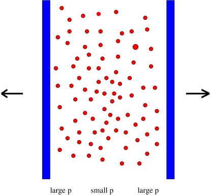
Figure 5: A hadron-hadron collision. The produced particles are shown as red circles.

The right moving particle which initiates the collision shown in Fig. 5 has $p_{1}^{+}\sim\sqrt{2}\mid p_{z}\mid$ and $p_{1}^{-}\sim{1\over{2\sqrt{2}}}m_{T}^{2}/\mid p_{z}\mid$. For the colliding particles $m_{T}=m_{projectile}$, that is because the transverse momentum is zero, the transverse mass equals the particle mass. For particle 2, we have $p^{+}_{2}=p^{-}_{1}$ and $p^{-}_{2}=p^{+}_{1}$.

If we define the Feynman $x$ of a produced pion as

$$x=p^{+}_{\pi}/p_{1}^{+}$$ (5)

then $0\leq x\leq 1$. (This definition agrees with Feynman’s original one if the energy of a particle in the center of mass frame is large and the momentum is positive. We will use this definition as a generalization of the original one of Feynman since it is invariant under longitudinal Lorentz boosts.) The rapidity of a pion is defined to be

$$y={1\over 2}ln(p^{+}_{\pi}/p^{-}_{\pi})={1\over 2}ln(2p^{+2}/m_{T}^{2})$$ (6)

For pions, the transverse mass includes the transverse momentum of the pion.

The pion rapidity is always in the range $-y_{CM}\leq y\leq y_{CM}$ where $y_{CM}=ln({p^{+}/m_{projectile}})$ All the pions are produced in a distribution of rapidities within this range.

A distribution of produced particles in a hadronic collision is shown in Fig. 6. The leading particles are shown in blue and are clustered around the projectile and target rapidities. For example, in a heavy ion collision, this is where the nucleons would be. In red, the distribution of produced mesons is shown.

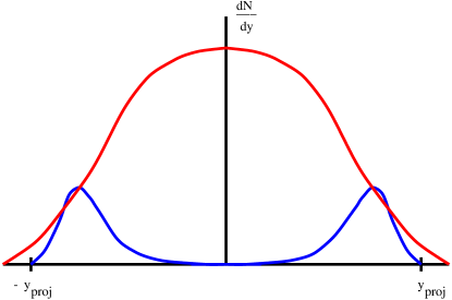
Figure 6: The rapidity distribution of particles produced in a hadronic collision.

These definitions are useful, among other reasons, because of their simple properties under longitudinal Lorentz boosts: $p^{\pm}\rightarrow\kappa^{\pm 1}p^{\pm}$ where $\kappa$ is a constant. Under boosts, the rapidity just changes by a constant.

The distribution of mesons, largely pions, shown in Fig. 4. are conveniently thought about in the center of mass frame. Here we imagine the positive rapidity mesons as somehow related to the right moving particle and the negative rapidity particles as related to the left moving particles. We define $x=p^{+}/p^{+}_{projectile}$ and $x^{\prime}=p^{-}/p^{-}_{projectile}$ and use $x$ for positive rapidity pions and $x^{\prime}$ for negative rapidity pions.

Several theoretical issues arise in multiparticle production. Can we compute $dN/dy$? or even $dN/dy$ at $y=0$? How does the average transverse momentum of produced particles $<p_{T}>$ behave with energy? What is the ratio of produced strange/nonstrange mesons, and corresponding ratios of charm, top, bottom etc at $y=0$ as the center of mass energy approaches infinity?

Does multiparticle production as $E\rightarrow\infty$ at $y=0$ become simple, understandable and computable?

There is a remarkable feature of rapidity distributions of produced hadrons, which we shall refer to as Feynman scaling. If we plot rapidity distributions of produced hadrons at different energies, then as function of the distance from the fragmentation region, the rapidity distributions are to a good approximation independent of energy. This is illustrated in Fig. 7. This means that as we go to higher and higher energies, the new physics is associated with the additional degrees of freedom at small rapidities in the center of mass frame (small-x degrees of freedom). The large x degrees of freedom do not change much. This suggests that there may be some sort of renormalization group description in rapidity where the degrees of freedom at larger x are held fixed as we go to smaller values of x. We shall see that in fact these large x degrees of freedom act as sources for the small x degrees of freedom, and the renormalization group is generated by integrating out low x degrees of freedom to generate these sources.

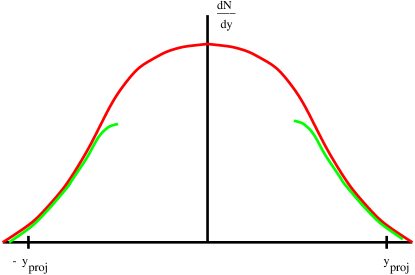
Figure 7: Feynman scaling of rapidity distributions. The two different colors correspond to rapidity distributions at different energies.

1.5 Deep Inelastic Scattering

In Fig. 2, deep inelastic scattering is shown. Here an electron emits a virtual photon which scatters from a quark in a hadron. The momentum and energy transfer of the electron is measured, and the results of the break up are not. In these lectures, I do not have sufficient time to develop the theory of deep inelastic scattering. Suffice it to say, that this measurement is sufficient at large momenta transfer $Q^{2}$ to measure the distributions of quarks in a hadron.

To describe the quark distributions, it is convenient to work in a reference frame where the hadron has a large longitudinal momentum $p^{+}_{hadron}$. The corresponding light cone momentum of the constituent is $p^{+}_{constituent}$. We define $x=p^{+}_{constituent}/p^{+}_{hadron}$. This x variable is equal to the Bjorken x variable, which can be defined in a frame independent way. In this frame independent definition, $x=Q^{2}/2p\cdot Q$ where $p$ is the momentum of the hadronic target and $Q$ is the momentum of the virtual photon. The cross section which one extracts in deep inelastic scattering can be related to the distributions of quarks inside a hadron, $dN/dx$.

It is useful to think about the distributions as a function of rapidity. We define this for deep inelastic scattering as

$$y=y_{hadron}-ln(1/x)$$ (7)

and the invariant rapidity distribution as

$$dN/dy=xdN/dx$$ (8)

Figure 8: The rapidity distribution of gluons inside of a hadron.

In Fig. 8, a typical $dN/dy$ distribution for constituent gluons of a hadron is shown. This plot is similar to the rapidity distribution of produced particles in deep inelastic scattering. The main difference is that we have only half of the plot, corresponding to the left moving hadron in a collision in the center of mass frame.

We shall later argue that there is in fact a relationship between the structure functions as measured in deep inelastic scattering and the rapidity distributions for particle production. We will argue that the gluon distribution function is in fact proportional to the pion rapidity distribution.

The small x problem is that in experiments at Hera, the rapidity distribution function for quarks grows as the rapidity difference between the quark and the hadron grows. This growth appears to be more rapid than simply $\mid y_{proj}-y\mid$ or $(y_{proj}-y)^{2}$, and various theoretical models based on the original considerations of Lipatov and colleagues suggest it may grow as an exponential in $\mid y_{proj}-y\mid$.bfkl (Consistency of the BFKL approach with the more established DGLAP evolution equations remains an outstanding theoretical problem.dglap ) If the rapidity distribution grew at most as $y^{2}$, then there would be no small x problem. We shall try to explain the reasons for this later in this lecture.

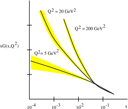
Figure 9: The Zeus data for the gluon structure functions.

In Fig. 9, the Zeus data for the gluon structure function is shown.z I have plotted the structure function for $Q^{2}=5~{}GeV^{2}$, $20~{}GeV^{2}$ and $200~{}GeV^{2}$. The structure function depends upon the resolution of the probe, that is $Q^{2}$. Note the rise of $xg(x)$ at small x, this is the small x problem. If one had plotted the total multiplicity of produced particles in $pp$ and $\overline{p}p$ collisions on the same plot, one would have found rough agreement in the shape of the curves. Here I would use $y=log(E_{cm}/1~{}GeV)$ for the pion production data. This is approximately the maximal value of rapidity difference between centrally produced pions and the projectile rapidity. The total multiplicity would be rescaled so that at small x, it matches the gluon structure functions. This demonstrates the qualitative similarity between the gluon structure function and the total multiplicity.

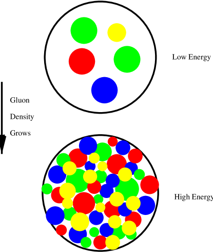
Figure 10: Saturation of gluons in a hadron. A view of a hadron head on as x decreases.

Why is the small x rise in the gluon distribution a problem? Consider Fig. 10, where we view hadron head on.glr -mq The constituents are the valence quarks, gluons and sea quarks shown as colored circles. As we add more and more constituents, the hadron becomes more and more crowded. If we were to try to measure these constituents with say an elementary photon probe, as we do in deep inelastic scattering, we might expect that the hadron would become so crowded that we could not ignore the shadowing effects of constituents as we make the measurement. (Shadowing means that some of the partons are obscured by virtue of having another parton in front of them. For hard spheres, for example, this would result in a decrease of the scattering cross section relative to what is expected from incoherent independent scattering.)

In fact, in deep inelastic scattering, we are measuring the cross section for a virtual photon $\gamma^{*}$ and a hadron, $\sigma_{\gamma^{*}hadron}$. Making x smaller corresponds to increasing the energy of the interaction (at fixed $Q^{2}$). An exponential growth in the rapidity corresponds to power law growth in $1/x$, which in turn implies power law growth with energy. This growth, if it continues forever, violates unitarity. The Froissart bound will allow at most $ln^{2}(1/x)$. (The Froissart bound is a limit on how rapidly a total cross section can rise. It follows from the unitarity of the scattering matrix.)

We shall later argue that in fact the distribution functions at fixed $Q^{2}$ do in fact saturate and cease growing so rapidly at high energy. The total number of gluons however demands a resolution scale, and we will see that the natural intrinsic scale is growing at smaller values of x, so that effectively, the total number of gluons within this intrinsic scale is always increasing. The quantity

$$\Lambda^{2}={1\over{\pi R^{2}}}{{dN}\over{dy}}$$ (9)

defines this intrinsic scale. Here $\pi R^{2}$ is the cross section for hadronic scattering from the hadron. For a nucleus, this is well defined. For a hadron, this is less certain, but certainly if the wavelengths of probes are small compared to $R$, this should be well defined. If

$$\Lambda^{2}>>\Lambda^{2}_{QCD}$$ (10)

as the Hera data suggests, then we are dealing with weakly coupled QCD since $\alpha_{S}(\Lambda)<<1$.

Even though QCD may be weakly coupled at small x, that does not mean the physics is perturbative. There are many examples of nonperturbative physics at weak coupling. An example is instantons in electroweak theory, which lead to the violation of baryon number. Another example is the atomic physics of highly charged nuclei. The electron propagates in the background of a strong nuclear Coulomb field, but on the other hand, the theory is weakly coupled and there is a systematic weak coupling expansion which allows for computation of the properties of high Z (Z is the charge of the nucleus) atoms.

We call this assortment of gluons a Color Glass Condensate. The name follows from the fact that the gluons are colored, and we have seen that they are very dense. For massless particles we expect that the high density limit will be a Bose condensate. The phase space density will be limited by repulsive gluon interactions, and be of order $1/\alpha_{s}>>1$. The glass nature follows because these fields are produced by partons at higher rapidity, and in the center of mass frame, they are Lorentz time dilated. Therefore the induced fields at smaller rapidity evolve slowly compared to natural time scales. These fields are also disordered. These two properties are similar to that of a glass which is a disrodered material which is a liquid on long time scales and a solid on short ones.

If the theory is local in rapidity, then the only parameter which can determine the physics at that rapidity is $\Lambda^{2}$. Locality in rapidity means that there are not long range correlations in the hadronic wavefunction as a function of rapidity. In pion production, it is known that except for overall global conserved quantities such as energy and total charge, such correlations are of short range. Note that if only $\Lambda^{2}$ determines the physics, then in an approximately scale invariant theory such as QCD, a typical transverse momentum of a constituent will also be of order $\Lambda^{2}$. If $\Lambda^{2}>>1/R^{2}$, where $R$ is the radius of the hadron, then the finite size of the hadron becomes irrelevant. Therefore at small enough x, all hadrons become the same. The physics should only be controlled by $\Lambda^{2}$.

There should therefore be some equivalence between nuclei and say protons. When their $\Lambda^{2}$ values are the same, their physics should be the same. We can take an empirical parameterization of the gluon structure functions as

$${1\over{\pi R^{2}}}{{dN}\over{dy}}\sim{{A^{1/3}}\over x^{\delta}}$$ (11)

where $\delta\sim.2-.3$. This suggests that there should be the following correspondences:

• RHIC with nuclei $\sim$ Hera with protons

• LHC with nuclei $\sim$ Hera with nuclei

Estimates of the parameter $\Lambda$ for nuclei at RHIC energies give $\sim 1-2~{}Gev$, and at LHC $2-3~{}Gev$.

Since the physics of high gluon density is weak coupling we have the hope that we might be able to do a first principle calculation of

• the gluon distribution function

• the quark and heavy quark distribution functions

• the intrinsic $p_{T}$ distributions quarks and gluons

We can also suggest a simple escape from unitarity arguments which suggest that the gluon distribution function must not grow at arbitrarily small x. The point is that at smaller x, we have larger $\Lambda$ and correspondingly larger $p_{T}$. A typical parton added to the hadron has a size of order $1/p_{T}$. Therefore although we are increasing the number of gluons, we do it by adding in more gluons of smaller and smaller size. A probe of size resolution $\Delta x\geq 1/p_{T}$ at fixed $Q$ will not see partons smaller than this resolution size. They therefore do not contribute to the fixed $Q^{2}$ cross section, and there is no contradiction with unitarity.

1.6 Heavy Ion Collisions

Figure 11: A space-time figure for ultrarelativistic heavy ion collisions.

In Fig. 11, the standard lightcone cartoon of heavy ion collisions is shown.bj To understand the figure, imagine we have two Lorentz contracted nuclei approaching one another at the speed of light. Since they are well localized, they can be thought of as sitting at $x^{\pm}=0$, that is along the light cone, for $t<0$. At $x^{\pm}=0$, the nuclei collide. To analyze this problem for $t\geq 0$, it is convenient to introduce a time variable which is Lorentz covariant under longitudinal boosts

$$\tau=\sqrt{t^{2}-z^{2}}$$ (12)

and a space-time rapidity variable

$$\eta={1\over 2}ln\left({{t-z}\over{t+z}}\right)$$ (13)

For free streaming particles

$$z=vt={p_{z}\over E}t$$ (14)

we see that the space-time rapidity equals the momentum space rapidity

$$\eta=y$$ (15)

If we have distributions of particles which are slowly varying in rapidity, it should be a good approximation to take the distributions to be rapidity invariant. This should be valid at very high energies in the central region. By the correspondence between space-time and momentum space rapidity, it is plausible therefore to assume that distributions are independent of $\eta$. Therefore distributions are the same on lines of constant $\tau$, which is as shown in Fig. 11. At $z=0$, $\tau=t$, so that $\tau$ is a longitudinally Lorentz invariant time variable.

We expect that at very late times, we have a free streaming gas of hadrons. These are the hadrons which eventually arrive at our detector. At some earlier time, these particles decouple from a dense gas of strongly interacting hadrons. As we proceed earlier in time, at some time there is a transition between a gas of hadrons and a plasma of quarks and gluons. This may be through a first order phase transition where the system might exist in a mixed phase for some length of time, or perhaps there is a continuous change in the properties of the system

At some earlier time, the quarks and gluons of the quark-gluon plasma are formed. This is at RHIC energies, a time of the order of a Fermi, perhaps as small as $.1~{}Fermi$. As they form, the particles scatter from one another, and this can be described using the methods of transport theory. At some later time they have thermalized, and the system can be approximately described using the methods of perfect fluid hydrodynamics.

In the time between that for which the quarks and gluons have been formed and $\tau=0$, the particles are being formed. This is where the initial conditions for a hydrodynamic description are made.

In various levels of sophistication, one can compute the properties of matter made in heavy ion collisions at times later than the formation time. The problems are understood in principle for $\tau\geq\tau_{formation}$ if perhaps not in fact. Very little is known about the initial conditions.

In principal, understanding the initial conditions should be the simplest part of the problem. At the initial time, the degrees of freedom are most energetic and therefore one has the best chance to understand them using weak coupling methods in QCD.

There are two separate classes of problems one has to understand for the initial conditions. First the two nuclei which are colliding are in single quantum mechanical states. Therefore for some early time, the degrees of freedom must be quantum mechanical. This means that

$$\Delta z\Delta p_{z}\geq 1$$ (16)

Therefore classical transport theory cannot describe the particle down to $\tau=0$ since classical transport theory assumes we know a distribution function $f(\vec{p},\vec{x},t)$, which is a simultaneous function of momenta and coordinates. This can also be understood as a consequence of entropy. An initial quantum state has zero entropy. Once one describes things by classical distribution functions, entropy has been produced. Where did it come from?

Another problem which must be understood is classical charge coherence. At very early time, we have a tremendously large number of particles packed into a longitudinal size scale of less than a fermi. This is due to the Lorentz contraction of the nuclei. We know that the particles cannot interact incoherently. For example, if we measure the field due to two opposite charge at a distance scale $r$ large compared to their separation, we know the field falls as $1/r^{2}$, not $1/r$. On the other hand, in cascade theory, interactions are taken into account by cross sections which involve matrix elements squared. There is no room for classical charge coherence.

There are a whole variety of problems one can address in heavy ion collisions such

• What is the equation of state of strongly interacting matter?

• Is there a first order QCD phase transition?

These issues and others would take us beyond the scope of these lectures. The issues which I would like to address are related to the determination of the initial conditions, a problem which can hopefully be addressed using weak coupling methods in QCD.

1.7 Universality

There are two separate formulations of universality which are important in understanding small x physics.

The first is a weak universality. This is the statement that physics should only depend upon the variablemv

$$\Lambda^{2}={1\over{\pi R^{2}}}{{dN}\over{dy}}$$ (17)

As discussed above, this universality has immediate experimentalconsequences which can be directly tested.

The second is a strong universality which is meant in a statistical mechanical sense. At first sight it appears to be a formal idea with little relation to experiment. If it is however true, its consequences are very powerful and far reaching. What we shall mean by strong universality is that the effective action which describes small x distribution function is critical and at a fixed point of some renormalization group. This means that the behavior of correlation functions is given by universal critical exponents, and these universal critical exponents depend only on general properties of the theory such as the symmetries and dimensionality.

Since the correlation functions determine the physics, this statement says that the physics is not determined by the details of the interactions, only by very general properties of the underlying theory!

2 Lecture II: A Very High Energy Nucleus

In this lecture, I will consider the properties of a single nucleus.mv -k I will develop the theory of the small x part of the nucleus, the components most relevant in the high energy limit. I will begin with some general considerations. This will largely be done to develop approximations which will be useful later, and leads directly to the Color Glass description. I then present a brief review of light cone quantization. Finally, I turn to a computation of the color fields which describe the nuclear wavefunction at small x. I show that in a simple approximation for the Color Glass, one recovers saturation, and that the phase space density of the fields is of order $1/\alpha_{s}$ which is typical of a Bose condensate.

2.1 Approximations and the Color Glass

In the previous lecture, I argued that when we go to small x

$$\Lambda^{2}={1\over{\pi R^{2}}}{{dN}\over{dy}}>>\Lambda_{QCD}^{2}$$ (18)

that the theory is weakly coupled $\alpha_{s}(\Lambda)<<1$. The typical transverse momentum scale of constituents of this low x part of the hadron wavefunction is

$$p_{T}^{2}\sim\Lambda^{2}>>1/R_{had}^{2}$$ (19)

This equation means that the scale of transverse variation of the hadron is over much larger sizes than the transverse De Broglie wavelength. I can therefore treat the hadron as having a well defined size and collisions will have well defined impact parameter.

For our purposes, it is sufficient to treat the hadron as a thin sheet of infinite transverse extent. The transverse variation in radius can be reinserted in an almost trivial generalization of these considerations. The thinness of the sheet follows because I shall assume that the sources for the fields at small x come from partons at much larger $x$ which are Lorentz contracted to size scales much smaller than can be resolved.

Figure 12: A single nucleus in the infinite momentum frame as seen by a small x probe.

In Fig. 12, a nucleus in the infinite momentum frame is shown, within the approximations described above.

Recall from the first lecture, we introduced rapidities associated with produced particles in hadron-hadron collisions,

$$y = {1\over 2}ln(p^{+}/p^{-})=ln(\sqrt{2}p^{+}/M_{T})$$ (20)

$$= ln(\sqrt{2}p^{+}_{had}/M_{T})+ln(p^{+}/p^{+}_{had})\sim y_{had}-ln(1/x)$$

This expression shows that the rapidity of produced hadrons can be written in the form used to describe the rapidity of constituents of a hadron. If we were to think of both the constituents and produced partons as pions, they would be the same, or alternatively if we think of both the produced and constituent partons as gluons. We can convert to spacetime rapidity using the uncertainty relation $p^{\pm}x^{\mp}\sim 1$.

$$y\sim{1\over 2}ln(x^{-}/x^{+})\sim y_{had}-ln(x^{-}p^{+}_{had})$$ (21)

We have assumed in deriving this relationship that the typical values of the proper time $\tau=\sqrt{x^{+}x^{-}}$ are not large compared to natural scales such as a transverse mass. These relations argue that all rapidities, up to shifts of order one, are the same. We can identify all momentum-space and space-time rapidities! This has the profound consequence that at high energies momentum space and space-time are intrinsically correlated, and particles which arise from a localized region of momentum space rapidity also arise from a localized region of space-time rapidity.

Now we illustrate a high energy hadron in terms of space-time rapidity. This has the effect of spreading out the thin sheet shown in Fig. 12, as shown in Fig. 13. Note that the partons which are shown have an ordering in momentum space rapidity which corresponds to their coordinate space rapidity. Fast partons are to the left. In this Figure, I have drawn a tube

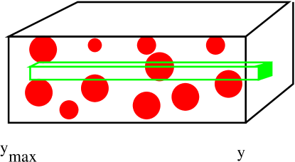
Figure 13: A single nucleus shown in terms of the space-time rapidity. The red circles indicate partons.

of transverse extent $dx$ which goes through the nucleus. I take $dx<<1~{}Fm$ so that one is resolving the constituents of ordinary hadrons. Notice that when $dx\rightarrow 0$, the longitudinal separation between hadrons which intersect the tube becomes large. If I also require that the energy is high enough so that there is always a large number of partons which intersect the box (which are longitudinally well separated), then one can think of a source associated with the charge inside the box, and this charge has a random distribution over the transverse area of the box. (At what scale the source becomes random is not entirely clear from this discussion. This will be resolved more carefully later.)

In the limit where $1/\Lambda<<dx<<1~{}Fm$, there are many charges inside the box of dimension $dx$. The charge should go over to a classical charge on this resolution scale because we can ignore commutators of charges

$$\mid[Q^{a},Q^{b}]\mid=\mid if^{abc}Q^{c}\mid<<Q^{2}$$ (22)

We can define a current associated with this charge which is localized in the sheet as

$$J^{\mu}_{a}=\delta^{\mu+}\delta(x^{-})q^{a}(x_{T})$$ (23)

The $+$ component of the current is the only important one because the sheet is traveling near the speed of light. The source $q^{a}(x_{T})$ is a c-number color charge density which is a random variable on the sheet. It is only defined on scales $1/\Lambda<<dx<<1~{}Fm$. The delta function of $x^{-}$ expresses the fact that the source is on a thin sheet. In fact, for many applications, we will have to relax the delta function assumption, and work with a charge density which includes the effect of distribution in $x^{-}$ as

$$q^{a}(x_{T})=\int dx^{-}~{}\rho^{a}(x^{-},x_{T})$$ (24)

and where for many purposes

$$\rho^{a}(x^{-},x_{T})\sim\delta(x^{-})q^{a}(x_{T})$$ (25)

We now know how to write down a theory. It is a theory where one computes the classical gluon field in stationary phase approximation and then integrates over a random source function. Its measure is

$$Z=\int[dA][d\rho]exp\left\{iS[A]+iJ^{+}A^{-}-{1\over 2}\int dx^{-}d^{2}x_{T}{{\rho^{2}(x^{-},x_{T})}\over{\mu^{2}(x^{-})}}\right\}$$ (26)

In this theory, we have assumed that the sources are randomly distributed as a Gaussian. This turns out to be an approximation valid in a particular range of resolution $dx$, and can be fixed up for a wider range. This will be discussed when we do the renormalization group. The sources and fields are coupled together in the standard $J\cdot A$ form. This results in the problem that the extended current conservation law $D_{\mu}J^{\mu}=0$ makes $J$ not an independent function. This problem can be avoided by introducing a generalization of the $J\cdot A$ coupling. This generalization turns out to be important for the renormalization group analysis of this theory, but is not important when we compute the classical field associated with these sources.

The above theory implicitly has cutoffs in it. We have discussed the range of $dx$ for which this effective theory is valid. Implicit in the analysis is that the fields we are computing have $p^{+}$ values much less than those of the sources. This implies there is an upper $p^{+}$ cutoff in the fields $A$ considered. If we were to Fourier analyze the sources $\rho$, they would have their support for $\mid p^{+}\mid$ which is greater than that of the cutoff. This cutoff is of course entirely arbitrary, and the lack of dependence of physical quantities upon this cutoff forms the basis of the renormalization group.

Notice that this theory, in spite of having a gauge dependent source, is gauge invariant on account of the integration over all sources. This computation of classical fields associated with sources and then averaging over sources is similar to the mathematics of glasses. The physical origin of this similarity is the Lorentz time dilation of the source for the fields and the disorder of the gluon field. The Lorentz time dilation is of course an approximation, and if one were to observe these classical fields over long enough time scales they would evolve, as do the atoms in a glass.

Notice that

$$<\rho^{a}(x)\rho^{b}(y)>=\delta^{ab}\delta^{(3)}(x-y)\mu^{2}(x^{-})$$ (27)

so that $\mu^{2}$ is the charge squared per unit transverse area per unit $x^{-}$ scaled by $1/(N_{c}^{2}-1)$.

2.2 Light Cone Quantization

Before discussing the properties of classical fields associated with these sources, it is useful to review some properties of light cone quantization.v This will allow us to pick out physical observables, such as the gluon density, from expectation values of gluon field operators.

Light cone coordinates are

$$x^{\pm}={1\over\sqrt{2}}(x^{0}\pm x^{3})$$ (28)

and momenta

$$p^{\pm}={1\over\sqrt{2}}(p^{0}\pm p^{3})$$ (29)

The invariant dot product is

$$p\cdot x=p_{t}\cdot x_{t}-p^{+}x^{-}-p^{-}x^{+}$$ (30)

where $p_{t}$ and $x_{t}$ are transverse coordinates. This implies that in this basis the metric is $g^{+-}=g^{-+}=-1$, $g^{ij}=\delta^{ij}$ where $i,j$ refer to transverse coordinates. All other elements of the metric vanish.

An advantage of light cone coordinates is that if we do a Lorentz boost along the longitudinal direction with Lorentz gamma factor $\gamma=cosh(y)$ then $p^{\pm}\rightarrow e^{\pm y}p^{\pm}$

If we let $x^{+}$ be a time variable, we see that the variable $p^{-}$ is to be interpreted as an energy. Therefore when we have a field theory, the component of the momentum operator $P^{-}$ will be interpreted as the Hamiltonian. The remaining variables are to be thought of as momenta and spatial coordinates. In Fig. 14, there is a plot of the $z,t$ plane. The line $x^{+}=0$ provides a surface where initial data might be specified. Time evolution is in the direction normal to this surface.

Figure 14: The initial value problem in light cone coordinates.

We see that an elementary wave equation

$$(p^{2}+M^{2})\phi=0$$ (31)

is particularly simple in light cone gauge. Since $p^{2}=p_{t}^{2}-2p^{+}p^{-}$ this equation is of the form

$$p^{-}\phi={{p_{t}^{2}+M^{2}}\over{2p^{+}}}\phi$$ (32)

is first order in time. In light cone coordinates, the dynamics looks similar to that of the Schrodinger equation. The initial data to be specified is only the value of the field on the initial surface.

In the conventional treatment of the Klein-Gordon field, one must specify the field and its first derivative (the momentum) on the initial surface. In light cone coordinates, the field is sufficient and the field momentum is redundant. This means that the field momentum will not commute with the field on the initial time surface!

Lets us work all this out with the example of the Klein Gordon field. The action for this theory is

$$S=-\int d^{4}x\left\{{1\over 2}(\partial\phi)^{2}+{1\over 2}M^{2}\phi^{2}\right\}$$ (33)

The field momentum is

$$\Pi(x_{t},x^{-})={{\delta S}\over{\delta\partial_{+}\phi}}=\partial_{-}\phi={\partial\over{\partial x^{-}}}\phi$$ (34)

Note that $\Pi$ is a derivative of $\phi$ on the initial time surface. It is therefore not an independent variable, as would be the case in the standard canonical quantization of the scalar field.

We postulate the equal time commutation relation

$$[\Pi(x_{t},x^{-}),\phi(y_{t},y^{-})]=-{i\over 2}\delta^{(3)}(x-y)$$ (35)

(The factor of two in the above expression is subtle and comes from a careful reduction of constrained Dirac bracket quantization for the classical theory to quantum field theory. It can be checked by verifying that we get the correct result for the Hamiltonian.) Here the time is $x^{+}=y^{+}=0$ in both the the field and field momentum. We see therefore that

$$\partial_{-}[\phi(\vec{x}),\phi(\vec{y})]=-{i\over 2}\delta^{(3)}(x-y)$$ (36)

or

$$[\phi(x),\phi(y)]=-{i\over 2}\epsilon(x^{-}-y^{-})\delta^{(2)}(x-y)$$ (37)

Here $\epsilon(v)$ is $1/2$ for $v>0$ and $-1/2$ for $v<0$.

These commutation relations may be realized by the field

$$\phi(x) = \int{{d^{3}p}\over{(2\pi)^{3}2\sqrt{2}p^{+}}}e^{ipx}a(p)$$ (38)

$$= \int_{p^{+}>0}{{d^{3}p}\over{(2\pi)^{3}2\sqrt{2}p^{+}}}\left\{e^{ipx}a(p)+e^{-ipx}a^{\dagger}(p)\right\}$$

Using

$$[a(p),a^{\dagger}(q)]=2p^{+}(2\pi)^{3}\delta^{(3)}(p-q)$$ (39)

one can verify that the equal time commutation relations for the field are satisfied.

The quantity $1/p^{+}$ in the expression for the field in terms of creation and annihilation operators is singular when $p^{+}=0$. When we use a principle value prescription, we reproduce the form of the commutation relations postulated above with the factor of $\epsilon(x^{-}-y^{-})$. Different prescriptions correspond to different choices for the inversion of $1\over\partial^{-}$. One possible prescription is the Leibbrandt-Mandelstam prescription $1/p^{+}=p^{-}/(p^{+}p^{-}+i\epsilon)$. This prescription has some advantages relative to the principle value prescription in that it maintains causality at intermediate stages of computations and the principle value prescription does not. In the end, for physical quantities, the choice of prescription cannot result in different results. Of course, in some schemes the computations may become prohibitively difficult.

The light cone Hamiltonian is

$$P^{-}=\int_{p^{+}>0}{{d^{3}p}\over{(2\pi)^{3}2p^{+}}}{{p_{t}^{2}+M^{2}}\over{2p^{+}}}a^{\dagger}(p)a(p)$$ (40)

with obvious physical interpretation.

In a general interacting theory, the Hamiltonian will of course be more complicated. The representation for the fields in terms of creation and annihilation operators will be the same as above. Note that all particles created by a creation operator have positive $P^{+}$. Therefore, since the vacuum has $P^{+}=0$, there can be no particle content to the vacuum. It is a trivial state. Of course this must be wrong since the physical vacuum must contain condensates such as the one responsible for chiral symmetry restoration. It can be shown that such non-perturbative condensates arise in the $P^{+}=0$ modes of the theory. We have not been careful in treating such modes. For perturbation theory, presumably to all orders, the above treatment is sufficient for our purposes.

2.3 Light Cone Gauge QCD

In QCD we have a vector field $A^{\mu}_{a}$. This can be decomposed into longitudinal and transverse parts as

$$A^{\pm}_{a}={1\over\sqrt{2}}(A^{0}_{a}\pm A^{z}_{a})$$ (41)

and the transverse as lying in the two dimensional plane orthogonal to the beam z axis. Light cone gauge is

$$A^{+}_{a}=0$$ (42)

In this gauge, the equation of motion

$$D_{\mu}F^{\mu\nu}=0$$ (43)

is for the $+$ component

$$D_{i}F^{i+}-D^{+}F^{-+}=0$$ (44)

which allows one to compute $A^{-}$ in terms of $A^{i}$ as

$$A^{-}={1\over\partial^{+2}}D^{i}\partial^{+}A^{i}$$ (45)

This equation says that we can express the longitudinal field entirely in terms of the transverse degrees of freedom which are specified by the transverse fields entirely and explicitly. These degrees of freedom correspond to the two polarization states of the gluons.

We therefore have

$$A^{i}_{a}(x)=\int_{p^{+}>0}{{d^{3}p}\over{(2\pi)^{3}2p^{+}}}\left(e^{ipx}a^{i}_{a}(p)+e^{-ipx}a^{i\dagger}_{a}(p)\right)$$ (46)

where

$$[a^{i}_{a}(p),a^{j\dagger}_{b}(q)]=2p^{+}\delta_{ab}\delta^{ij}(2\pi)^{3}\delta^{(3)}(p-q)$$ (47)

where the commutator is at equal light cone time $x^{+}$.

2.4 Distribution Functions

We would like to explore some hadronic properties using light cone field operators. For example, suppose we have a hadron and ask what is the gluon content of that hadron. Then we would compute

$${{dN_{gluon}}\over{d^{3}p}}=<h\mid a^{\dagger}(p)a(p)\mid h>$$ (48)

If we express this in terms of the gluon field, we find

$${{dN_{gluon}}\over{d^{3}p}}={{2p^{+}}\over{(2\pi)^{3}}}<h\mid A^{ia}(\vec{p},x^{+})A^{ia}(-\vec{p},x^{+})\mid h>$$ (49)

which can be related to the gluon propagator. The quark distribution for quarks of flavor $i$ (for the sum of quarks and antiquarks) would be given in terms of creation and annihilation operators for quarks as

$${{dN_{i}}\over{d^{3}p}}=<h\mid\{b_{i}^{\dagger}(p)b_{i}(p)+d_{i}^{\dagger}(p)d_{i}(p)\}\mid h>$$ (50)

where $b$ corresponds to quarks and $d$ to antiquarks. The creation and annihilation operators for quarks and gluons can be related to the quark coordinate space field operators by techniques similar to those above.v1

2.5 The Classical Gluon Field

To compute the gluon distribution function, we need the expectation value of the gluon field. To lowest order in weak coupling, this is given by computing the classical gluon field and then averaging over sources. The classical equation of motion is

$$D_{\mu}F^{\mu\nu}=\delta^{\nu+}\rho(x^{-},x_{T})$$ (51)

To solve this equation we shall work in the gauge ${\cal A}^{-}=0$, and then gauge rotate the solution back to lightcone gauge $A^{+}=0$. The solution in ${\cal A}^{-}=0$ gauge is

$${\cal A}^{i} = 0$$

$$-\nabla_{T}^{2}{\cal A}^{+} = {\overline{\rho}}$$ (52)

Here ${\overline{\rho}}=U^{\dagger}(x)\rho U(x)$ is the source which has been gauge rotated to this new gauge. Since the measure for integration over sources is gauge invariant, we do not have to distinguish between these sources since we can rotate one into the other.

To rotate back to lightcone gauge we use

$${\cal A}^{\mu}=U^{\dagger}A^{\mu}U+{i\over g}U^{\dagger}\partial^{\mu}U$$ (53)

so that the gauge rotation matrix $U$ is

$$\partial^{+}U=-igU{\cal A}^{+}$$ (54)

where

$${\cal A}^{+}=\alpha={1\over{-\nabla_{T}^{2}}}\nabla{\overline{\rho}}$$ (55)

The solution isk -mkmw

$$U^{\dagger}=Pexp\left\{ig\int^{x^{-}}_{x_{0}^{-}}dz^{-}\alpha(z^{-},x_{T})\right\}$$ (56)

There is a choice of boundary condition here associated with $x_{0}^{+}$. The ambiguity with this choice is associated with a residual gauge freedom. We shall resolve this by choosing retarded boundary conditions, $x_{0}^{-}\rightarrow-\infty$. This boundary condition lets us construct the solution for $U$ at some $x^{-}_{1}$ knowing only information about $\alpha$ for $x^{-}<x^{-}_{1}$.

The solution in light cone gauge is therefore

$$A^{+} = A^{-}=0$$

$$A^{i} = {i\over g}U\nabla^{i}U^{\dagger}$$ (57)

If $x^{-}$ is outside of the range of support of the source $\rho$, this can be written as

$$A^{i}=\theta(x^{-}){i\over g}V\nabla^{i}V^{\dagger}$$ (58)

where

$$V^{\dagger}(x_{T})=Pexp\left(ig\int^{\infty}_{-\infty}dz^{-}\alpha(z^{-},x_{T})\right)$$ (59)

We now have an explicit expression for the gluon field in terms of the sources.k ,mkmw For our Gaussian weight function, we can now compute the expectation value of the gluon fields which gives the gluon distribution function. The details of such a computation are given in Ref. mkmw . It is a straightforward computation to perform: One can expand out the exponentials and compute term by term in the expansion. The series exponentiates. One subtlety occurs due to logarithmic infrared infinity which is regulated on a scale of order of a Fermi where transverse charge correlations go to zero since all hadrons are color singlet.mah . The result is

$$<A^{i}_{a}(\vec{x},x^{+})A^{i}_{a}(\vec{0},x^{+})> = {{N_{c}^{2}-1}\over{\pi\alpha_{s}N_{c}}}{1\over x_{T}^{2}}\times$$ (60)

$$\left(1-exp\{x_{T}^{2}Q_{s}^{2}ln(x_{T}^{2}\Lambda_{QCD}^{2})/4\}\right)$$

In this equation, the saturation momentum is defined as

$$Q_{s}^{2}=2\pi N_{c}\alpha_{s}^{2}\int dx^{-}\mu^{2}$$ (61)

and is of the order $\alpha_{s}^{2}$ times the charge squared per unit area.

This expression can be Fourier transformed to produce the gluon distribution function, with result as shown in Fig. 15.

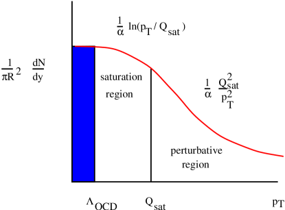
Figure 15: The gluon distribution function.

We can understand this plot from the properties of the coordinate space distribution function. We notice that the dominant scale factor in the problem is $Q_{s}$, so to a first approximation everything scales in terms of this quantity. Large $p_{T}$ corresponds to small $x_{T}$, and the coordinate space distribution behaves as $ln(x_{T}^{2})$ which corresponds to $1/p_{T}^{2}$. This is typical of a bremstrahlung spectrum. At larger $x_{T}$, distribution is of order $1/x_{T}^{2}$, which Fourier transforms into $ln(p_{T}^{2})$ at small $p_{T}$. The softer $x_{T}$ dependence at large $x_{T}$ can be traced to a dipole cancelation of the fields. The monopole charge field, seen at short distances is $ln(x_{T}^{2})$ and the dipole cancelation should set in at large distances when one cannot resolve individual charges, and reduce this by two powers of $x_{T}$.

The overall scale of the curve is $1/\alpha_{s}$. The quantity we are plotting is in fact the phase space density of gluons. At small $\alpha_{s}$, this density becomes large, and the Color Glass becomes a condensate. Hence the name, Color Glass Condensate.

This form of the gluon distribution function illustrates how the problems with unitarity can be solved. Let us assume that the saturation momentum $Q_{s}$ is rapidly increasing as $x\rightarrow 0$. If we start with an $x$ so that $Q>>Q_{s}$, then as $x$ decreases, the number of gluons which can be seen in scattering rises like $Q_{s}^{2}$. (See Fig. 15.) Eventually, $Q_{s}$ becomes larger than $Q$, in which case, the number of gluons rise slowly, like $ln(Q_{s})$. At this point the cross section saturates since the number of gluons which can be resolved stops growing, and we are consistent with unitarity constraints.

The gluon distribution function is defined to be

$$xG(x,Q^{2})=\int_{0}^{Q^{2}}d^{2}p_{T}{{dN}\over{d^{2}p_{T}dy}}$$ (62)

This behaves in the saturation region as $\pi R^{2}Q^{2}$, and in the large $Q$ region as $\pi R^{2}Q_{s}^{2}$. We expect that $Q_{s}^{2}\sim charge^{2}/area$ and due to the random nature of the way charges add, $Q_{s}^{2}\sim R$. Therefore in the saturation region, the gluon distribution function is proportional to the surface area of the hadron, that is the gluons can only be seen which are on the surface of the hadron. In the large $Q$ region, one sees gluons from the entire hadron, that is, the hadron has become transparent.

2.6 The Structure of the Gluon Field

The gluon field arises from a charge density which is essentially delta function in $x^{-}$. In order to solve the equations of motion, the field must have a discontinuity at $x^{-}=0$. This can be achieved with a field which is a two dimensional gauge transform of zero field strength on one side of the sheet and a different gauge transform of zero on the other side. The field strength $F^{\mu\nu}$ is therefore zero if $\mu$ and $\nu$ are both in the two dimensional transverse space. If either index is $-$, it also vanishes since there is no change in the $x^{+}$ direction. The only non-vanishing component is therefore $F^{i+}$, and this is a delta function in the $x^{-}$ direction. Since $F^{i\pm}=E^{i}\pm\epsilon^{ij}B^{j}$, we see that

$$\vec{E}\perp\vec{B}\perp\vec{z}$$ (63)

The fields are therefore transversely polarized to the direction of motion and live in the two dimensional sheet where the charges sit. These are the non-abelian generalizations of the Lienard-Wiechert potentials of electrodynamics. The density of these fields is of order $1/\alpha_{s}$. A picture of the Color Glass Condensate is shown in Fig. 16.

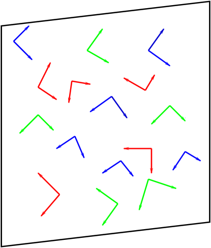
Figure 16: The non-abelian Lienard-Wiechert potentials which form the Color Glass Condensate.

3 Lecture III: Hadron-Hadron Collisions and the Initial Conditions for Heavy Ion Collisions

3.1 Phenomenology of Mini-Jets

In the last lecture, we argued that at small x, the typical gluon constituent of a hadron acquires a transverse momentum of order $Q_{s}$, and that this can grow as $x\rightarrow 0$. This leads us to hope that in hadron-hadron collisions, this will be the typical momentum scale of particle production. If true, then the processes are weakly coupled and computable using weak coupling methods.

This is reminiscent of past attempt to compute particle production by mini-jetskaj -xnwang . On dimensional grounds, the cross section for jet production $d\sigma/dyd^{2}p_{T}\sim\alpha_{s}^{2}/p_{T}^{4}$. If we attempt to compute the total cross section for jet production,

$${{d\sigma}\over{dy}}\sim\alpha_{s}^{2}\int_{\Lambda^{2}_{QCD}}{{d^{2}p_{T}}\over p_{T}^{4}}$$ (64)

the result is infrared sensitive, and presumably would be cutoff at $\Lambda_{QCD}$. In early computations, one introduced an ad hoc cutoff which was fixed, and hopefully large enough so that one could compute the minijet component. This of course left unanswered many questions about the origin of this cutoff, and the effects of particles produced below the cutoff scale.

In this lecture, we will argue that the Color Glass Condensate cuts off the integral at a scale of order $Q_{s}$, the saturation momentum. At large $p_{T}$, dimensional arguments tell us that the density of produced particles has the form

$${1\over{\pi R^{2}}}{{dN}\over{d^{2}p_{T}dy}}=\kappa{1\over\alpha_{s}}{Q_{s}^{4}\over p_{T}^{4}}$$ (65)

The factor of $1/p_{T}^{4}$ comes about because the high $p_{T}$ tail is controlled by perturbation theory. The $1/\alpha_{s}$ arises because of the large density of gluons in the condensate. In fact, if we can successfully formulate the particle production problem classically, we expect that in general

$${1\over{\pi R^{2}}}{{dN}\over{d^{2}p_{T}dy}}={1\over\alpha_{s}}F(Q_{s}^{2}/p_{T}^{2})$$ (66)

At large $p_{T}>>Q_{s}$, $F\sim Q_{s}^{4}/p_{T}^{4}$ and for small $p_{T}<<Q_{s}$, $F$ should be slowly varying (logarithmic) or a constant. A plot is shown in Fig. 17.

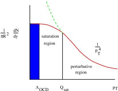
Figure 17: The $p_{T}$ distribution for mini-jets produced by a Color Glass Condensate.

A word of caution should be injected about the interpretation of mini-jet production. Typically it is assumed that there is a simple relationship between the multiplicity of produced gluon jets and the multiplicity of pions. Usually, $N_{pion}$ is taken to be some constant of order one times $N_{gluon}$. In our considerations, we can only talk about the gluon mini-jet production, and it is beyond the scope of these lectures to relate this to the final state multiplicity. Suffice it to say that the situation is controversial, particularly in heavy ion collisions where there can be much final state interaction.son .

Recall that in heavy ion collisions, we expect that $Q_{s}^{2}\sim A^{1/3}$. At large $p_{T}$, Eqn. 66 predicts that

$${{dN}\over{d^{2}p_{T}dy}}\sim\pi R^{2}{Q_{s}^{4}\over p_{T}^{4}}\sim{A^{4/3}\over p_{T}^{4}}$$ (67)

This result is consistent with hard incoherent scattering. At small $p_{T}$,

$${{dN}\over{d^{2}p_{T}dy}}\sim\pi R^{2}\sim A^{2/3}$$ (68)

which is consistent with much shadowing, and the gluons are produced from the surface of the nuclei.

The total multiplicity per unit rapidity

$${{dN}\over{dy}}\sim R^{2}\int_{Q_{s}^{2}}d^{2}p_{T}{{Q_{s}^{4}}\over p_{T}^{4}}\sim R^{2}Q_{s}^{2}\sim A$$ (69)

is proportional to $A$, just as in color string models! This is because for the Color Glass Condensate, the cutoff in transverse momentum depends on $A$. (If one was careful with the factors of $\alpha_{s}$ in the above equation, one would predict mild logarithmic modifications of the linear dependence on $A$.) In addition to the $A$ dependence, there is also a correlation between the energy dependence of the gluon distribution function at saturation and the multiplicity of minijets since

$$\pi R^{2}Q_{s}^{2}=\int_{x}^{1}dx^{\prime}G(x^{\prime},Q_{s})$$ (70)

a relationship which follows from the last lecture.

We can be a little more careful with the numerical factors which determine the saturation momentum.mclgyu Using the results of last lecture,

$$Q_{s}^{2}={{2\pi N_{c}\alpha_{s}^{2}}\over{\pi R^{2}(N_{c}^{2}-1)}}Q_{color}^{2}$$ (71)

Here $Q_{color}^{2}$ is the color charge squared of all quarks and gluons at larger $x$ values than that of interest. For a quark,

$$Q_{quark}^{2}={1\over{N_{c}(N_{c}^{2}-1)}}tr~{}\tau_{a}^{2}={1\over{2N_{c}}}$$ (72)

and for a gluon

$$Q_{gluon}^{2}={N_{c}\over{(N_{c}^{2}-1)}}$$ (73)

We find that

$$Q_{color}^{2}={N_{quark}\over{2N_{c}}}+{{N_{c}N_{gluon}}\over{(N_{c}^{2}-1)}}$$ (74)

If we plug in numbers, at RHIC energies corresponding to $x\sim 10^{-2}$, $Q_{s}\sim 1-2~{}GeV$

3.2 Classical Description of Hadron Collisions

We want to describe the collision of two ultra-relativistic hadrons. A collision is shown in Fig. 18. The hadrons have been Lorentz contracted to thin sheets and a Color Glass Condensate sits in the planes of both sheets.

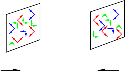
Figure 18: A collision of two ultra-relativistic hadrons.

Before the collision the non-zero fields are for right moving nucleus, $F^{i+}\sim\delta(x^{-})$ and for the left moving nucleus $F^{i-}\sim\delta(x^{+})$. Before the nuclei pass through one another, nothing happens and the fields in each sheet are static. When they pass through one another, the sum of these two fields is not a solution of the equations of motion, unlike the case in electrodynamics, and this induces a time evolution of the fields.kmw

One can understand this from the vector potentials. In Fig. 19

Figure 19: A space-time diagram for the vector potentials in hadron-hadron scattering.

a space-time diagram is shown for the scattering. In the backward light cone, Region I, the field is a pure two dimensional gauge transform of zero field. In crossing into Regions II and III, the fields must have a discontinuity to match the charge on the surfaces of the lightcone. This requires the vector potential to be different gauge transforms of zero field strength, $G_{2}$ and $G_{3}$ in these regions. Now in going to Region IV, one could solve either for the sources on the left edge of the forward light cone with a gauge transform of zero or the right edge of the forward light cone with a different gauge transform of zero. One cannot satisfy the equations of motion for the fields in the presence of the sources on both edges of the light cones with the same gauge transform of zero field strength. One must produce a field in the forward light cone which is not a gauge, and therefore matter is produced.

The situation in QCD is completely different than that in electrodynamics. In electrodynamics, one must produce pairs of charged particles to make matter in the forward light cone. This arises from a quantum correction to the equations of motion. In QCD, matter is produced classically.

The procedure for solving this problem is now straightforward, in principle. One solves the classical equations of motion in the forward light cone with boundary conditions at the edges of the forward light cone. We will shortly determine these boundary conditions and the form of the solution in the forward light cone. Then one evolves the equations of motion into the far future. At some time, the energy density becomes dilute, and the field equations should linearize in some gauge. One can then identify the quanta of the linearized fields in the standard way that one does classical radiation theory in electrodynamics.

3.3 The Form of the Classical Field

Before the collision, the form of the classical field can be taken as

$$A^{+} = A^{-}=0$$

$$A^{i} = \theta(x^{-})\theta(-x^{+})\alpha^{i}_{1}(x_{T})+\theta(-x^{-})\theta(x^{+})\alpha^{i}_{2}(x_{T})$$ (75)

where the $\alpha^{i}$ are two dimensional gauge transforms of zero field. We will consider the collision of identical hadrons. The solution in the forward light cone is therefore expected to be boost invariant. After the collision, a boost invariant solution is

$$A^{+} = x^{+}\alpha(\tau,x_{T})$$

$$A^{-} = x^{-}\beta(\tau,x_{T})$$

$$A^{i} = \alpha^{i}_{3}(\tau,x_{T})$$ (76)

We can choose the gauge

$$x^{+}A^{-}+x^{-}A^{+}=0$$ (77)

so that

$$\alpha(\tau,x_{T})=-\beta(\tau,x_{T})$$ (78)

In the forward light cone, the equations of motion are

$${1\over\tau^{3}}\partial_{\tau}\tau^{3}\partial_{\tau}\alpha-[D^{i},[D^{i},\alpha]]=0$$ (79)

and

$${1\over\tau}\partial_{\tau}\tau\partial_{\tau}\alpha^{i}_{3}-ig\tau^{2}[\alpha,[D^{i},\alpha]]-[D^{j},F^{ji}]=0$$ (80)

The boundary conditions are determined by matching the solution in Regions II and III to that in the forward light cone. The result is that $\alpha$ and $\alpha^{i}_{3}$ must both be regular as $\tau\rightarrow 0$ and

$$\alpha_{3}^{i}(0,x_{T}) = \alpha_{1}^{i}(x_{T})+\alpha_{2}^{i}(x_{T})$$

$$\alpha(0,x_{T}) = {{-ig}\over 2}[\alpha^{i}_{1}(x_{T}),\alpha_{2}^{i}(x_{T})]$$ (81)

The problem is now well defined, and these equations may be numerically solved.

The behaviour of these solution at large $\tau$ can be extracted. With $V(x_{T})$ an element of the group, the solution is a small fluctuation field up to a possible large gauge transformation

$$\alpha(\tau,x_{T}) = V\epsilon(\tau,x_{T})V^{\dagger}$$

$$\alpha^{i}_{3}(\tau,x_{T}) = V(\epsilon^{i}_{3}(\tau,x_{T})+{i\over g}\partial^{i})V^{\dagger}$$ (82)

The small fluctuation fields $\epsilon$ and $\epsilon^{i}$ solve the equations

$${1\over\tau^{3}}\partial_{\tau}\tau^{3}\partial_{\tau}\epsilon-\nabla^{2}_{T}\epsilon=0$$ (83)

and

$${1\over\tau}\partial_{\tau}\tau\partial_{\tau}\epsilon^{i}-(\nabla^{2}_{T}\delta^{ij}-\nabla^{i}\nabla^{j})\epsilon^{j}=0$$ (84)

At large $\tau$, these linear equations can be Fourier analyzed with the result

$$\epsilon^{a}(\tau,x_{T})=\int{{d^{2}k_{T}}\over{(2\pi)^{2}\sqrt{2\omega}}}{1\over\tau^{3/2}}\left(a_{1}^{a}(k_{T})e^{-ik\cdot x}+c.c.\right)$$ (85)

and

$$\epsilon^{ai}(\tau,x_{T})=\int{{d^{2}k_{T}}\over{(2\pi)^{2}\sqrt{2\omega}}}\epsilon^{ij}{k^{j}\over\omega}{1\over\tau^{1/2}}\left(a_{2}^{a}(k_{T})e^{-ik\cdot x}+c.c.\right)$$ (86)

In these equations $\omega=\mid k_{T}\mid$.

One can compute the energy distribution associated with these fields as

$${{dE}\over{dyd^{2}k_{T}}}={\omega\over{(2\pi)^{2}}}\sum_{ia}\mid a_{i}^{a}(k_{T})\mid^{2}$$ (87)

and the multiplicity distribution is given by dividing this by $\omega$, that is

$${{dN}\over{dyd^{2}k_{T}}}={1\over{(2\pi)^{2}}}\sum_{ia}\mid a_{i}^{a}(k_{T})\mid^{2}$$ (88)

These last two formulae correspond to those of free quantum filed theory when we replace $a(p),a^{*}(p)$ by the creation and annihilation operators $a(p),a^{\dagger}(p)$. The $a(p)$ are the classical quantities which correspond to the quantum creation and annihilation operators. These formulae show how to use the classical solutions to compute distributions of produced minijets.

3.4 Numerical Results for Mini-Jet Production

Krasnitz and Venugopalan have numerically solved the classical equations for mini-jet production.kv This involves finding a gauge invariant discretization of the classical equations of motion. One then solves the classical equations for a fixed $\rho_{1}$ and $\rho_{2}$, and extracts the produced radiation. An ensemble of sources are produced with the Gaussian weight of the Color Glass, which then produces an ensemble of radiation fields. These fields are then averaged to generate the mini-jet distributions.

In Fig. 20, the form of the numerical results for mini-jet production is illustrated. At large $p_{T}$, the results of analytic studies are reproduced which up to logarithms is $\sim 1/p^{4}_{T}$. At $p_{T}\leq Q_{s}$, the distribution flattens out.kmw -mclgyu

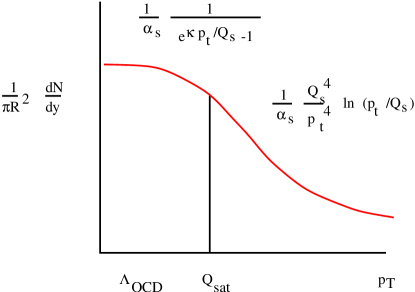
Figure 20: An illustration of the results generated by numerical simulation of the classical equations for mini-jet production.

To good numerical accuracy, the result in this region can be fit to a two dimensional Bose Einstein distribution,

$${1\over{\pi R^{2}}}{{dN}\over{d^{2}p_{T}dy}}\sim{1\over\alpha_{s}}{1\over{e^{\kappa p_{T}/Q_{s}}-1}}$$ (89)

where $\kappa$ is a constant of order 1.

The result at large $p_{T}$ can be computed analytically by expanding the equations in powers of the gluon field. At high $p_{T}$, the phase space is not so heavily occupied, so a field strength expansion makes sense. At small $p_{T}$, it is not at all certain that the result is in fact an exact two dimensional Bose-Einstein distribution.kv -ksea In any case, the origins of this distribution have nothing at all to do with thermodynamics, and it is a useful example of the traps one can fall into if one assumes that exponential distribution corresponds to a temperature and thermalization.

3.5 pA Scattering

An interesting example of minijet production is given by the collision of two hadrons of different size.kovmu -dumcl We will generically refer to this as $pA$ scattering, although most of our considerations could be generalized to $A^{\prime}A$ nuclear collisions. In Fig. 21,

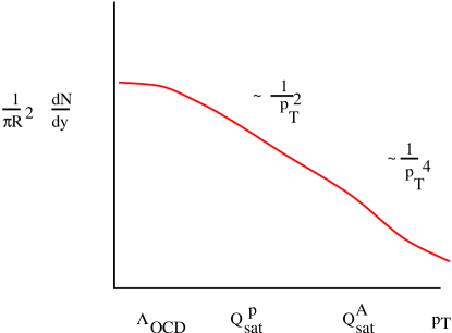
Figure 21: The $p_{T}$ distribution for particles produced in a $pA$ collision.

the transverse momentum distribution for $pA$ scattering is shown.

There are three distinct regions, which follow from the fact that there are two saturation scales, $Q_{s}^{A}$ and $Q_{s}^{p}$, and $Q_{s}^{p}<<Q_{s}^{A}$ since $(Q_{s}^{A})^{2}\sim A^{1/3}$. At very large $p_{T}$ where the fields from both nuclei are small, the distribution can be computed from perturbation theory, and the distribution falls as $1/p_{T}^{4}$ and is proportional to $(Q^{A}_{s}Q^{p}_{s})^{2}$. This first region is for $p_{T}>>Q_{s}^{A}$. An intermediate region where the field from the nucleus is strong but the field from the proton is weak and can be treated perturbatively. This intermediate region is for $Q_{s}^{p}<<p_{T}<<Q_{s}^{A}$. There is finally the region where $p_{T}<<Q_{s}^{p}$ where both fields are strong.

We expect that in the intermediate region, the transverse momentum dependence will be in between the flat behaviour at small $p_{T}$ and the $1/p_{T}^{4}$ behaviour characteristic of large $p_{T}$, The naive expectation is $1/p_{T}^{2}$ in the intermediate region. The total multiplicity can be computed if one understands this intermediate region since the dominant contribution arises here. The strength in this intermediate region should involve the total charge squared from the proton, but that from the nucleus should go like $p_{T}^{2}$ so that when combined with the $1/p_{T}^{4}$, one gets a distribution proportional to $1/p_{T}^{2}$. This softer behaviour of the distribution function follows since we are inside the region where we expect coherence from the field of the nucleus, and since the distribution should extrapolate between $1/p_{T}^{4}$ at very large $p_{T}$ and a constant, up to logarithms, at very small $p_{T}$.

In fact, it is possible to compute the behaviour in this intermediate region. The equations for the classical production can be analytically solved for any $p_{T}>>Q_{s}^{A}$. The solution in the forward light cone are plane waves which are gauge transformed by the field of the large nucleus. The boundary conditions determine the strength of these waves.

For the total multiplicity, in the large $p_{T}$ region $dN/dyd^{2}p_{T}\sim A^{1/3}$. We expect that as we interpolate between the proton fragmentation region and that of the nucleus, we go between $O(1)$ and $O(A^{1/3})$ as shown in Fig. 22.

Figure 22: The distribution in rapidity for $dN/dyd^{2}p_{T}$ in a $pA$ collision.

For $p_{T}$ in the intermediate region, we expect that $dN/dyd^{2}p_{T}$ is of order 1 except for a small region of rapidity around the fragmentation region of the nucleus. The total integrated multiplicity arises from this latter region so we expect that $dN/dy\sim O(1)$.

3.6 Thermalization

After the gluons are produced in hadron-hadron collisions, they may rescatter from one another.son If one goes to very small x so that the density of gluons becomes very large, one expects that the gluons will eventually thermalize. Due to the very large typical $p_{T}$, $\alpha_{s}<<1$, and this takes a time $\tau\sim 1/(\alpha_{s}^{2}Q_{s})$ which is longer by a factor of $1/\alpha_{s}^{2}$ than the natural time scale. The system therefore becomes dilute relative to its natural scale.

In the first diagram of Fig. 23, there is ordinary Coulomb scattering. When all processes which populate and depopulate phase space are summed, this diagram is only naively logarithmically divergent, and is cutoff by the density dependent Debye mass. $\rho_{gluons}<<p_{T}^{3}$.

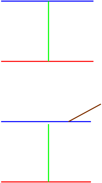
Figure 23: The diagrams for gluon scattering which lead to thermalization.

In the second diagram, there is no such cancellation, and the diagram is of order $1/(\alpha_{s}\sqrt{\rho_{gluons}})$. At a time of order $1/(\alpha_{s}^{2}Q_{s})$ for a density decreasing like $1/\tau$ as we expect for ultrarelativistic nuclear collisions, the diagram is enhanced by a factor of $1/\alpha_{s}$. This cancels the extra factor of $\alpha_{s}$ coming from the diagram being higher order in perturbation theory.son .

What appears to happen is that as the system gets more dilute, it thermalizes due to multigluon production. This will modify the relationship between the number of gluons produced as mini-jets and the pion multiplicity. How this actually works is not yet fully understood.

4 Lecture 4: The Renormalization Group

The effective action for the theory we have described must be gauge invariant and properly describe the dynamics in the presence of external sources. For the theory which we have written down in past lectures with the $J\cdot A$ coupling of source to field, gauge invariance is only retained if we impose

$$D_{\mu}J^{\mu}=0$$ (90)

This equation presents a problem in our formulation since it implies that the source cannot be independently specified from the field. This did not present a problem for the classical theory since one could find a solution which solved the constraint. When we compute quantum corrections and proceed to a renormalization group treatment, we must be more careful.

In a clever series of papers,mklw it was shown that one can generalize the $J\cdot A$ coupling. This lead Jalilian-Marian, Kovner, Leonidov and Weigert to propose the action

$$S = -{1\over 4}\int d^{4}xF_{\mu\nu}^{a}F_{a}^{\mu\nu}+{i\over N_{c}}\int d^{2}x_{t}dx^{-}\delta(x^{-})$$ (91)

$$\times\rho^{a}(x_{t})trT^{a}exp\left\{i\int_{-\infty}^{\infty}dx^{+}T\cdot A^{-}(x)\right\}$$

In this equation, the matrix $T$ is in the adjoint representation of the gauge group. This is required for reality of the action. When this action is extremized to get the Yang-Mills equations, one can identify the current and show that the current is covariantly conserved. This action is invariant under gauge transformations which are identified at $x^{+}=\pm\infty$. (Even this can be corrected to get a fully invariant theory if one generalizes even further to complex time Keldysh contours. As shown in Ref. ilm , this further generalization does not affect the renormalization group in lowest non-trivial order.) This is a consequence of the gauge invariance of the measure of integration over the sources $\rho$. This will be taken as a boundary condition on the theory. In general if we had not integrated over sources, one could not define a gauge invariant theory with a source, as gauge rotations would change the definition of the source. Here because the source is integrated over in a gauge invariant way, the problem does not arise.

In the most general gauge invariant theory which we can write down is generated from

$$Z=\int[d\rho]e^{-F[\rho]}\int[dA]e^{iS[A,\rho]}$$ (92)

This is a generalization of the Gaussian ansatz described in the previous lecture. It allows for a slightly more complicated structure of stochastic variation of the sources. The Gaussian ansatz can be shown to be valid when evaluating structure functions at large transverse momenta.

$$F_{Gaussian}[\rho]={1\over 2}\int dx^{-}d^{2}x_{t}~{}{{\rho^{2}(x_{t})}\over{\mu^{2}(x^{-})}}$$ (93)

This theory is an effective theory valid only in a limited range of rapidity much less than the rapidity of the source. The sources for this theory sit at higher rapidity. This happens because as we go to lower values of rapidity, the fluctuations in the field are integrated out and are replaced by sources and an integral over fluctuations in the source. The renormalization group equations which we will describe are what make the theory independent of this cutoff. To fully determine $F$ in the above equation demands a full solution of these renormalization group equations. This has yet to be done, although there are now approximate solutions for small and large transverse momentum of the fields.ilm -im

We can understand this a little better by imagining what happens when we compute a quantum correction to the classical theory. This quantum correction will generate terms proportional to $\alpha_{s}ln(\Lambda^{+}/p^{+})$ where $\Lambda^{+}$ is the $p^{+}$ cutoff for our effective theory. Clearly these corrections are small and sensible only if $e^{-1/\alpha_{s}}\Lambda^{+}<<p^{+}<<\Lambda^{+}$. If we want to generate a good effective theory at smaller values of $p^{+}$, we need to break the theory into intervals of $p^{+}$ with each interval sufficiently small so that the quantum fluctuations are small and computable. The relation between one interval and the next is the renormalization group.

The remarkable thing that happens when one integrates out the fluctuations interval is that only the function $F$ which controls the source strength is modified! The functional form of $F$ is modified so that this equation is of the form

$${d\over{dy}}Z=-H(\rho,\delta/\delta\rho)Z$$ (94)

where

$$y=ln(\Lambda^{+}_{i}/\Lambda^{+}_{f})$$ (95)

and $\Lambda^{+}_{i,f}$ are the cutoffs at the initial and final values, and

$$Z=e^{-F}$$ (96)

This equation is of the form of the time evolution for a two spatial dimension quantum field theory where the coordinates are $\rho$ and the momenta are $d/d\rho$.

4.1 How to Compute the RG Effective Hamiltonian

In the Eqn. 94, the renormalization group Hamiltonian H was introduced. I will here outline how it is computed. We first take the theory defined for $p^{+}<\Lambda^{+}_{i}$. We integrate out the quantum fluctuations. In particular, the two point function is

$${\cal G}^{ij}(x,y)=<(A^{i}(x)+\delta A^{i}(x))(A^{i}(y)+\delta A^{i}(y))>$$ (97)

In this equation, $A$ is the classical background field and $\delta A$ is the small fluctuation. At the momentum scales which will be of interest for $p^{+}<\Lambda^{+}_{f}$, it is sufficient to consider the equal time limit of this correlation function. We now identify

$$<\delta A\delta A> = G<\delta\rho\delta\rho>G$$ (98)

$$= G\chi G$$

where $G$ is the Greens function in the classical background field $A$. We also identify

$$<\delta A> = G<\delta\rho>$$ (99)

$$= \sigma$$

We can get exactly the same result by modifying the weight function so that we reproduce $\chi$ and $\sigma$ and move the cutoff to $\Lambda^{+}_{f}$ so that there are no longer quantum fluctuations to integrate out. This is the origin of the form of Eqn. 94

Some technical comments about the computations are required. One must be extremely careful of gauge. The gauge prescriptions of retarded or advanced for $1/k^{+}$ singularities are used. We were not able to effectively use either Leibbrandt-Mandelstam or principle value prescriptions although this may be possible in principle. When one computes propagators in background fields, one gets analytic expressions in terms of line ordered phases of the source $\rho$. It is most convenient to compute these in $\delta A^{-}=0$ gauge and express things in terms of the source in $A^{-}=0$ gauge, and then rotate results back to lightcone gauge. This can be carefully done only when the $1/k^{+}$ singularity is properly regularized.

If we change variable to space-time rapidity, we can define

$$\alpha(y,x_{T})={1\over{-\nabla_{T}^{2}}}\rho(y,x_{T})$$ (100)

and

$$V^{\dagger}(y,x_{T})=Pexp\left(ig\int_{-\infty}^{y}dy^{\prime}\alpha(y^{\prime},x_{T})\right)$$ (101)

After much work, one finds

$$H={\alpha_{s}\over 2}\int d^{2}x_{T}J^{ia}(x_{T})J^{ia}(x_{T})$$ (102)

where

$$J^{ia}(x_{T})=\int{{d^{2}z_{T}}\over\pi}{{(x-z)^{i}}\over{(x-z)^{2}}}(1-V^{\dagger}(y,x_{T})V(y,z_{T}))^{ab}{1\over i}{\delta\over{\delta\alpha^{b}(y,z_{T})}}$$ (103)

The Hamiltonian is positive definite and looks like a pure kinetic energy term (up to the multiplicative non-linearities) with no potential.ilm

The renormalization group above can also be seen to be a consequence of equations for correlation functions of $V(y,x_{T})$.bal In Ref. kmiw it was shown that these equations for correlation functions were almost the same as those of the renormalization group. There was an error in this analysis associated with the subtleties of gauge fixing, and when repaired gives that these equations are precisely equivalent.ilm . Meanwhile, Weigert showed that the equations for the correlation functions could be summarized as a Hamiltonian equation of the form above.weig which was also shown to be precisely the equations for the renormalization group Hamiltonian.ilm

4.2 Quantum Diffusion

The Hamiltonian presented in the previous section is analogous to that without a potential. If we were to ignore the non-linearities associated with the matrices $V$, this would be the Hamiltonian for a free theory with only momenta and no potential.

If there was a potential in the Hamiltonian, then at large times, the solution of the above renormalization group equations would be trivial,

$$Z\sim exp(-yE_{o})$$ (104)

where $E_{o}$ is the ground state energy. All expectation values would become rapidity independent and the solution to the small $x$ problem would be trivial: $x$ independence.

The solution to the above equation is more complicated. One can see this by studying a one dimensional quantum mechanics problem:

$${d\over{dy}}Z=-{p^{2}\over 2}Z$$ (105)

with solution

$$Z={1\over\sqrt{2\pi y}}exp(-x^{2}/2y)$$ (106)

This equation describes diffusion. The width of the Gaussian in $x$ grows with time. This is unlike solving

$${d\over{dy}}Z=-\left({p^{2}\over 2}+V(x)\right)Z$$ (107)

In this latter case, the coordinate $x$ evolves towards the minimum of $V$, and then does undergo small fluctuations around this minimum.

We see therefore that the non-triviality of the small x problem in QCD arises because of the quantum diffusive nature of the renormalization group equations.

4.3 Some Generic Features of the Renormalization Group Equation

If we compute the correlation function of two sources using Eqn. 94, we find that

$${d\over{dy}}<\rho(x)\rho(y)>=-<\rho(x)\rho(y)H>$$ (108)

At large $k_{T}$ when the fields are linear, the gluon structure function is the same as the source-source correlation function up to a trivial factor of $1/k_{T}^{2}$. (The momenta $k_{T}$ is conjugate to the coordinate $x_{T}-y_{T}$.) If we ignore the non-linearities in $H$, keeping the lowest order non-vanishing terms, and if we integrate by parts the factors of $\delta/\delta\alpha(y,x_{T})$, we get a closed linear equation for the correlation function. This is precisely the BFKL equation.

In fact, in the region where the equations are linear, one is in the high $k_{T}$ limit, and this also reduces to the DGLAP and BFKL equations, which are known to be equivalent if one computes distribution functions to leading order in $\alpha_{s}ln(1/x)ln(Q^{2})$, where $Q$ is some typical momentum for the correlation function, $Q\sim k_{T}$. When the non-linearities are important, the non-linearities of this equation cannot be ignored.

The situation is as shown in Fig. 24.

Figure 24: The various regions of evolution for structure functions in the $ln(1/x)$-$ln(Q^{2})$ plane.

In the linear region, one can choose to evolve using linear equations. In the $ln(Q^{2})$ direction, the equation is the DGLAP equation and in the $ln(1/x)$ direction, it is the BFKL equation. There is a boundary region in the $ln(1/x)$-$ln(Q^{2})$ plane. Within this boundary region, there is a high density of glue and the evolution becomes non-linear. One always collides with this region if one decreases $x$ and holds $Q^{2}$ fixed or decreases $Q^{2}$ holding $x$ fixed.

4.4 Some Limiting Solutions of the Renormalization Group Equations

In the small $k_{T}$ region, we expect that correlation functions such as $<V(x)V^{\dagger}(y)>$ are very small, since we are probing the theory at distance scales long compared to natural correlation lengths. In this limit, one might be able to ignore the non-linearities in the renormalization group equations. Using that $x^{i}/x^{2}=\nabla^{i}/\nabla^{2}$, we have then

$$\int d^{2}x_{T}~{}J^{2}(x_{T})\sim\int d^{2}zd^{2}z^{\prime}<z\mid{1\over{-\nabla_{T}^{2}}}\mid z^{\prime}>{\delta\over{\delta\alpha(y,z)}}{\delta\over{\delta\alpha(y,z^{\prime})}}$$ (109)

The solution for Eqn. 94 is

$$F={\kappa\over{2\alpha_{s}}}\int dyd^{2}x_{T}\nabla_{T}^{i}\alpha(y,x_{T})\nabla_{T}^{i}\alpha(y,x_{T})$$ (110)

The small $k_{T}$ functional $F$ is a pure scale-invariant Gaussian. It is universal and independent of initial conditions.

In the large $p_{T}$ region, we perform a mean field analysis. The result is that discussed in Lecture II.

For details of the analysis leading to the results of this section, the interested reader is referred to im .

4.5 Some Speculative Remarks

The form of the renormalization group equation appears to be simple. It looks like it might even be possible to find exact solutions. In remarkable works,bal ,k2 Balitsky and Kovchegov have shown that the equation for the two line correlation function $W(x)W^{\dagger}(y)$ where $W$ is in the fundamental representation becomes a closed non-linear equation in the large $N_{color}$ limit. This means that at large $N_{color}$ one can compute this correlation function at arbitrarily small x including all the non-linearities associated with small x.

Although Kovchegov’s original derivation was for large nuclei, the result can be shown to follow directly from the renormalization group Eqn. 94. This is done by taking the expectation value of $<W(x)W^{\dagger}(y)>$, using the form of the Hamiltonian and a factorization property of expectation values true in large $N_{color}$. A derivation is presented in Ref. im for the interested reader.

This result is interesting in itself since it means that all of the saturation effects for $F_{2}(x,Q^{2})$ may be computed at small $x$. The Balitsky-Kovchegov equation has been solved numerically.braun

More important, it suggests that perhaps, at least in large $N_{color}$, the full renormalization group equations may be solved for $F$.

5 Concluding Comments

In these lectures, constraints of space and time have forced me to not mention many of the exciting areas that are currently under study. One of these areas, is diffraction.buchmuller -kovmcl . One can show that the same formalism which gives deep inelastic scattering also gives diffraction and that there is a simple relation between diffractive structure functions and deep inelastic scattering. I have also not developed a formal treatment of deep inelastic scattering within the Color Glass Condensate picture.mueller -venmcl .

The last lecture is very sketchy, and should provide an introduction to the literature on this problem. The derivation of the results discussed in that lecture are onerous, and all the details have been omitted in these lectures. In some sense this is good, since the most interesting part of this problem is to understand and solve the renormalization group equations, and at least this problem is clearly stated, and free from the technical details from which it arises..

An area which should be better understood from the perspective presented above is the nature of shadowing for nuclei at small x. This relates deep inelastic scattering and diffraction in a non-trivial way, and the Color Glass Condensate is one of the few theories available which pretends to treat both consistently.

The other area where there is much potential is the production of quarks in hadron-hadron collisions. In particular, the charm quark may provide us a real clue about non trivial dynamics since its mass is very close to the scale of the Color Glass Condensate for large nuclei at accessible energies.

6 Acknowledgments

These lectures were delivered at the 40’th Schladming Winter School: DENSE MATTER, March 3-10, 2001. I thank the organizers for making this a very informative meeting, with an excellent atmosphere for interaction.

I thank my colleagues Alejandro Ayala-Mercado, Adrian Dumitru, Elena Ferreiro, Miklos Gyulassy, Edmond Iancu Yuri Kovchegov, Alex Kovner, Jamal Jalilian-Marian, Andrei Leonidov, Raju Venugopalan and Heribert Weigert with whom the ideas presented in this talk were developed. I particularly thank Kazunori Itakura for a careful and critical reading of the manuscript.

This manuscript has been authorized under Contract No. DE-AC02-98H10886 with the U. S. Department of Energy.

References

- (1) L. N. Lipatov, Sov. J. Nucl. Phys. 23, 338 (1976); E.A. Kuraev, L.N. Lipatov and Y.S. Fadin, Zh. Eksp. Teor. Fiz 72, 3 (1977) (Sov. Phys. JETP 45, 1 (1977) ); Ya. Ya. Balitsky and L.N. Lipatov, Sov. J. Nucl. Phys. 28 822 (1978);
- (2) V. Gribov and L. Lipatov, Sov. Journ. Nucl. Phys. 15, 438 (1972); G. Altarelli and G. Parisi, Nucl. Phys. B126 298 (1977); Yu.L. Dokshitser, Sov.Phys.JETP 46 641 (1977).
- (3) J. Breitweg et. al., Eur. Phys. J. 67, 609 (1999) and references therein.
- (4) L. V. Gribov, E. M. Levin and M. G. Ryskin, Phys. Rep. 100 1 (1983).
- (5) A. H. Mueller and Jian-wei Qiu, Nucl. Phys. B268, 427 (1986).
- (6) J. D. Bjorken, Phys. Rev. D27, 140 (1983).
- (7) L. McLerran and R. Venugopalan, Phys. Rev. D49 2233 (1994); D49 3352 (1994).
- (8) A. H. Mueller, Nucl. Phys. B558, 285 (1999).
- (9) Y. Kovchegov, Phys. Rev. D54, 5463 (1996); D55, 5445 (1997).
- (10) R. Venugopalan nucl-th/9808023.
- (11) L. McLerran and R. Venugopalan, Phys. Rev. D50, 2225 (1994).
- (12) J. Jalilian-Marian, A. Kovner, L. McLerran and H. Weigert, Phys. Rev. D55 5414 (1997);
- (13) C. S. Lam and G. Mahlon, Phys. Rev. D62, 114023 (2000).
- (14) K. Kajantie, P. Landshoff and J. Lindfors, Phys. Rev. Lett. 59, 2527 (1987); K. Eskola, K. Kajnatie and J. Lindfors, Nucl. Phys. B323, 327 (1989).
- (15) M. Gyulassy and Xin-Nian Wang, Phys. Rev. D43, 104 (1991).
- (16) R. Baier, A. Mueller, D. Schiff and D. Son, Phys. Lett. B502, 51 (2001)
- (17) M. Gyulassy and L. McLerran, Phys. Rev. C56 2219 (1997).
- (18) A. Kovner, L. McLerran, and H. Weigert Phys. Rev. D52, 3809 (1995); 6231 (1995).
- (19) A. Krasnitz and R. Venugopalan Phys. Rev. Lett. 84, 4309 (2000); Nucl. Phys. B557, 237 (1999).
- (20) S. Bass, B. Muller and W. Poschl, J. Phys. G25, L109 (1999)
- (21) Y. Kovchegov, hep-ph/0011252.
- (22) Y. Kovchegov and A. H. Mueller, Nucl. Phys. B529, 451 (1998).
- (23) D. Rischke and Y. Kovchegov, Phys. Rev. C56, 1084 (1997)
- (24) A. Dumitru and L. McLerran, in preparation.
- (25) J. Jalilian-Marian, A. Kovner, A. Leonidov and H. Weigert Nucl. Phys. B504 415 (1997); Phys. Rev. D59 014014 (1999); J. Jalilian-Marian, A. Kovner and H. Weigert, Phys. Rev. D59 014015 (1999).
- (26) E. Iancu and L. McLerran, hep-ph/0103032.
- (27) E. Iancu, A. Leonidov and L. McLerran, hep-ph/0012009; hep-ph/0011241; E. Ferreiro, E. Iancu, A. Leonidov and L. McLerran, in preparation.
- (28) I. Balitsky, Nucl. Phys. B463, 99 (1996).
- (29) A. Kovner, J. G. Milhano and H. Weigert, Phys. Rev. D62, 114005 (2000)
- (30) H. Weigert, hep-ph/0004044.
- (31) Y. Kovchegov, Phys. Rev. D60, 034008 (1999); D61, 074018 (2000).
- (32) M. Braun Eur. Phys. J. C16, 337 (2000).
- (33) W. Buchmuller, T. Gehrmann and A. Hebecker, Nucl. Phys. B537, 477 (1999).
- (34) L. Mclerran and Y. Kovchegov Phys. Rev. D60, 054025 (1999).
- (35) A. H. Mueller, Nucl. Phys. B307, 34 (1988); B317, 573 (1989); B335, 115 (1990).
- (36) L. McLerran and R. Venugopalan, Phys. Rev. D59, 094002 (1999).