Transverse Polarisation of Quarks in Hadrons

Abstract

We review the present state of knowledge regarding the transverse polarisation (or transversity) distributions of quarks. After some generalities on transverse polarisation, we formally define the transversity distributions within the framework of a classification of all leading-twist distribution functions. We describe the QCD evolution of transversity at leading and next-to-leading order. A comprehensive treatment of non-perturbative calculations of transversity distributions (within the framework of quark models, lattice QCD and QCD sum rules) is presented. The phenomenology of transversity (in particular, in Drell–Yan processes and semi-inclusive leptoproduction) is discussed in some detail. Finally, the prospects for future measurements are outlined.

Contents

toc

1 Introduction

There has been, in the past, a common prejudice that all transverse spin effects should be suppressed at high energies. While there is some basis to such a belief, it is far from the entire truth and is certainly misleading as a general statement. The main point to bear in mind is the distinction between transverse polarisation itself and its measurable effects. As well-known, even the ultra-relativistic electrons and positrons of the LEP storage ring are significantly polarised in the transverse plane [1] due to the Sokolov–Ternov effect [2]. Thus, the real problem is to identify processes sensitive to such polarisation: while this is not always easy, it is certainly not impossible.

Historically, the first extensive discussion of transverse spin effects in high-energy hadronic physics followed the discovery in 1976 that $\Lambda^{0}$ hyperons produced in $pN$ interactions even at relatively high $p_{T}$ exhibit an anomalously large transverse polarisation [3]. This result implies a non-zero imaginary part of the off-diagonal elements of the fragmentation matrix of quarks into $\Lambda^{0}$ hyperons. It was soon pointed out that this is forbidden in leading-twist quantum chromodynamics (QCD), and arises only as a $\mathop{\mathcal{O}}\nolimits(1/p_{T})$ effect [6, 7, 8]. It thus took a while to fully realise that transverse spin phenomena are sometimes unsuppressed and observable.

The subject of this report is the transverse polarisation of quarks. This is an elusive and difficult to observe property that has escaped the attention of physicists for many years. Transverse polarisation of quarks is not, in fact, probed in the cleanest hard process, namely deeply-inelastic scattering (DIS), but is measurable in other hard reactions, such as semi-inclusive leptoproduction or Drell–Yan dimuon production.

At leading-twist level, the quark structure of hadrons is described by three distribution functions: the number density, or unpolarised distribution, $f(x)$; the longitudinal polarisation, or helicity, distribution $\Delta{f}(x)$; and the transverse polarisation, or transversity, distribution $\Delta_{T}{f}(x)$.

The first two are well-known quantities: $f(x)$ is the probability of finding a quark with a fraction $x$ of the longitudinal momentum of the parent hadron, regardless of its spin orientation; $\Delta{f}(x)$ measures the net helicity of a quark in a longitudinally polarised hadron, that is, the number density of quarks with momentum fraction $x$ and spin parallel to that of the hadron minus the number density of quarks with the same momentum fraction but spin antiparallel. If we call $f_{\pm}(x)$ the number densities of quarks with helicity ${\pm}1$, then we have

$$f(x) = f_{+}(x)+f_{-}(x)\,,$$ (1.0.1a)

$$\Delta{f}(x) = f_{+}(x)-f_{-}(x)\,.$$ (1.0.1b)

The third distribution function, $\Delta_{T}{f}(x)$, although less familiar, also has a very simple meaning. In a transversely polarised hadron $\Delta_{T}{f}(x)$ is the number density of quarks with momentum fraction $x$ and polarisation parallel to that of the hadron, minus the number density of quarks with the same momentum fraction and antiparallel polarisation, i.e.,

$$\Delta_{T}{f}(x)=f_{\uparrow}(x)-f_{\downarrow}(x)\,.$$ (1.0.2)

In a basis of transverse polarisation states $\Delta_{T}{f}$ too has a probabilistic interpretation. In the helicity basis, in contrast, it has no simple meaning, being related to an off-diagonal quark-hadron amplitude.

Formally, quark distribution functions are light-cone Fourier transforms of connected matrix elements of certain quark-field bilinears. In particular, as we shall see in detail (see Sec. 4.2), $\Delta_{T}{f}$ is given by (we take a hadron moving in the $z$ direction and polarised along the $x$-axis)

$$\Delta_{T}{f}(x)=\int\!\frac{\d\xi^{-}}{4\pi}\,\e^{\text{i}xP^{+}\xi^{-}}\langle PS|\mathchoice{\makebox[0.0pt][l]{$\displaystyle\kern 2.08334pt\overline{\kern-2.43059pt\phantom{\psi}}$}}{\makebox[0.0pt][l]{$\textstyle\kern 2.08334pt\overline{\kern-2.43059pt\phantom{\psi}}$}}{\makebox[0.0pt][l]{$\scriptstyle\kern 1.45834pt\overline{\kern-1.7014pt\phantom{\psi}}$}}{\makebox[0.0pt][l]{$\scriptscriptstyle\kern 1.04167pt\overline{\kern-1.21529pt\phantom{\psi}}$}}\psi(0)\text{i}\sigma^{1+}\gamma_{5}\psi(0,\xi^{-},\mathchoice{\mbox{\boldmath$\displaystyle 0$\unboldmath}}{\mbox{\boldmath$\textstyle 0$\unboldmath}}{\mbox{\boldmath$\scriptstyle 0$\unboldmath}}{\mbox{\boldmath$\scriptscriptstyle 0$\unboldmath}}_{\perp})|PS\rangle\,.$$ (1.0.3)

In the parton model the quark fields appearing in (1.0.3) are free fields. In QCD they must be renormalised (see Sec. 5.1). This introduces a renormalisation-scale dependence into the parton distributions:

$$f(x)\,,\,\Delta{f}(x)\,,\,\Delta_{T}{f}(x)\to f(x,\mu^{2})\,,\,\Delta{f}(x,\mu^{2})\,,\,\Delta_{T}{f}(x,\mu^{2})\,,$$ (1.0.4)

which is governed by the Dokshitzer-Gribov-Lipatov-Altarelli-Parisi [10, 11, 12, 13] (DGLAP) equations (see Sec. 5).

It is important to appreciate that $\Delta_{T}{f}(x)$ is a leading-twist quantity. Hence it enjoys the same status as $f(x)$ and $\Delta{f}(x)$ and, a priori, there is no reason that it should be much smaller than its helicity counterpart. In fact, model calculations show that $\Delta_{T}{f}(x)$ and $\Delta{f}(x)$ are typically of the same order of magnitude, at least at low $Q^{2}$, where model pictures hold (see Sec. 8).

The QCD evolution of $\Delta_{T}{f}(x)$ and $\Delta{f}(x)$ is, however, quite different (see Sec. 5.4). In particular, at low $x$, $\Delta_{T}{f}(x)$ turns out to be suppressed with respect to $\Delta{f}(x)$. As we shall see, this behaviour has important consequences for some observables. Another peculiarity of $\Delta_{T}{f}(x)$ is that it has no gluonic counterpart (in spin-${\textstyle\frac{1}{2}}$ hadrons): gluon transversity distributions for nucleons do not exist (Sec. 4.5). Thus $\Delta_{T}{f}(x)$ does not mix with gluons in its evolution, and evolves as a non-singlet quantity.

Figure 1: (a) Representation of the chirally-odd distribution $\Delta_{T}{f}(x)$. (b) A handbag diagram forbidden by chirality conservation.

One may wonder why the transverse polarisation distributions are so little known, if they are quantitatively comparable to the helicity distributions. No experimental information on $\Delta_{T}{f}(x)$ is indeed available at present (see, however, Sec. 9.2.2, where mention is made of some preliminary data on pion leptoproduction that might involve $\Delta_{T}{f}(x)$). The reason has already been mentioned: transversity distributions are not observable in fully inclusive DIS, the process that has provided most of the information on the other distributions. Examining the operator structure in (1.0.3) one can see that $\Delta_{T}{f}(x)$, in contrast to $f(x)$ and $\Delta{f}(x)$, which contain $\gamma^{+}$ and $\gamma^{+}\gamma_{5}$ instead of $\text{i}\sigma^{1+}\gamma_{5}$, is a chirally-odd quantity (see Fig. 1a). Now, fully inclusive DIS proceeds via the so-called handbag diagram which cannot flip the chirality of the probed quark (see Fig. 1b). In order to measure $\Delta_{T}{f}$ the chirality must be flipped twice, so one needs either two hadrons in the initial state (hadron–hadron collisions), or one hadron in the initial state and one in the final state (semi-inclusive leptoproduction), and at least one of these two hadrons must be transversely polarised. The experimental study of these processes has just started and will provide in the near future a great wealth of data (Sec. 9).

So far we have discussed the distributions $f(x)$, $\Delta{f}(x)$ and $\Delta_{T}{f}(x)$. If quarks are perfectly collinear, these three quantities exhaust the information on the internal dynamics of hadrons. If we admit instead a finite quark transverse momentum $\mathchoice{\mbox{\boldmath$\displaystyle k$\unboldmath}}{\mbox{\boldmath$\textstyle k$\unboldmath}}{\mbox{\boldmath$\scriptstyle k$\unboldmath}}{\mbox{\boldmath$\scriptscriptstyle k$\unboldmath}}_{\perp}$, the number of distribution functions increases (Sec. 4.7). At leading twist, assuming time-reversal invariance, there are six $\mathchoice{\mbox{\boldmath$\displaystyle k$\unboldmath}}{\mbox{\boldmath$\textstyle k$\unboldmath}}{\mbox{\boldmath$\scriptstyle k$\unboldmath}}{\mbox{\boldmath$\scriptscriptstyle k$\unboldmath}}_{\perp}$-dependent distributions. Three of them, called in the Jaffe–Ji–Mulders classification scheme [14, 15] $f_{1}(x,\mathchoice{\mbox{\boldmath$\displaystyle k$\unboldmath}}{\mbox{\boldmath$\textstyle k$\unboldmath}}{\mbox{\boldmath$\scriptstyle k$\unboldmath}}{\mbox{\boldmath$\scriptscriptstyle k$\unboldmath}}_{\perp}^{2})$, $g_{1L}(x,\mathchoice{\mbox{\boldmath$\displaystyle k$\unboldmath}}{\mbox{\boldmath$\textstyle k$\unboldmath}}{\mbox{\boldmath$\scriptstyle k$\unboldmath}}{\mbox{\boldmath$\scriptscriptstyle k$\unboldmath}}_{\perp}^{2})$ and $h_{1}(x,\mathchoice{\mbox{\boldmath$\displaystyle k$\unboldmath}}{\mbox{\boldmath$\textstyle k$\unboldmath}}{\mbox{\boldmath$\scriptstyle k$\unboldmath}}{\mbox{\boldmath$\scriptscriptstyle k$\unboldmath}}_{\perp}^{2})$, upon integration over $\mathchoice{\mbox{\boldmath$\displaystyle k$\unboldmath}}{\mbox{\boldmath$\textstyle k$\unboldmath}}{\mbox{\boldmath$\scriptstyle k$\unboldmath}}{\mbox{\boldmath$\scriptscriptstyle k$\unboldmath}}_{\perp}^{2}$, yield $f(x)$, $\Delta{f}(x)$ and $\Delta_{T}{f}(x)$, respectively. The remaining three distributions are new and disappear when the hadronic tensor is integrated over $\mathchoice{\mbox{\boldmath$\displaystyle k$\unboldmath}}{\mbox{\boldmath$\textstyle k$\unboldmath}}{\mbox{\boldmath$\scriptstyle k$\unboldmath}}{\mbox{\boldmath$\scriptscriptstyle k$\unboldmath}}_{\perp}$, as is the case in DIS. Mulders has called them $g_{1T}(x,\mathchoice{\mbox{\boldmath$\displaystyle k$\unboldmath}}{\mbox{\boldmath$\textstyle k$\unboldmath}}{\mbox{\boldmath$\scriptstyle k$\unboldmath}}{\mbox{\boldmath$\scriptscriptstyle k$\unboldmath}}_{\perp}^{2})$, $h_{1L}^{\perp}(x,\mathchoice{\mbox{\boldmath$\displaystyle k$\unboldmath}}{\mbox{\boldmath$\textstyle k$\unboldmath}}{\mbox{\boldmath$\scriptstyle k$\unboldmath}}{\mbox{\boldmath$\scriptscriptstyle k$\unboldmath}}_{\perp}^{2})$ and $h_{1T}^{\perp}(x,\mathchoice{\mbox{\boldmath$\displaystyle k$\unboldmath}}{\mbox{\boldmath$\textstyle k$\unboldmath}}{\mbox{\boldmath$\scriptstyle k$\unboldmath}}{\mbox{\boldmath$\scriptscriptstyle k$\unboldmath}}_{\perp}^{2})$. If time-reversal invariance is not applied (for the physical motivation behind this, see Sec. 4.8), two more, $T$-odd, $\mathchoice{\mbox{\boldmath$\displaystyle k$\unboldmath}}{\mbox{\boldmath$\textstyle k$\unboldmath}}{\mbox{\boldmath$\scriptstyle k$\unboldmath}}{\mbox{\boldmath$\scriptscriptstyle k$\unboldmath}}_{\perp}$-dependent distribution functions appear [16]: $f_{1T}^{\perp}(x,\mathchoice{\mbox{\boldmath$\displaystyle k$\unboldmath}}{\mbox{\boldmath$\textstyle k$\unboldmath}}{\mbox{\boldmath$\scriptstyle k$\unboldmath}}{\mbox{\boldmath$\scriptscriptstyle k$\unboldmath}}_{\perp}^{2})$ and $h_{1}^{\perp}(x,\mathchoice{\mbox{\boldmath$\displaystyle k$\unboldmath}}{\mbox{\boldmath$\textstyle k$\unboldmath}}{\mbox{\boldmath$\scriptstyle k$\unboldmath}}{\mbox{\boldmath$\scriptscriptstyle k$\unboldmath}}_{\perp}^{2})$. At present the existence of these distributions is merely conjectural.

To summarise, here is an overall list of the leading-twist quark distribution functions:

$$\overbrace{f\,,\;\Delta{f}\,,\;\Delta_{T}{f}\vphantom{{}^{\perp}}}^{\text{no $\mathchoice{\mbox{\boldmath$\displaystyle k$\unboldmath}}{\mbox{\boldmath$\textstyle k$\unboldmath}}{\mbox{\boldmath$\scriptstyle k$\unboldmath}}{\mbox{\boldmath$\scriptscriptstyle k$\unboldmath}}_{\perp}$}}\,,\,\overbrace{g_{1T}\,,\;h_{1L}^{\perp}\,,\;h_{1T}^{\perp}}^{\!\text{$\mathchoice{\mbox{\boldmath$\displaystyle k$\unboldmath}}{\mbox{\boldmath$\textstyle k$\unboldmath}}{\mbox{\boldmath$\scriptstyle k$\unboldmath}}{\mbox{\boldmath$\scriptscriptstyle k$\unboldmath}}_{\perp}$-dependent}\!}\,,\,\underbrace{f_{1T}^{\perp}\,,\;h_{1}^{\perp}\rule[-4.30554pt]{0.0pt}{0.0pt}}_{\text{$T$-odd}}\,.$$

At higher twist the proliferation of distribution functions continues [14, 15]. Although, for the sake of completeness, we shall also briefly discuss the $\mathchoice{\mbox{\boldmath$\displaystyle k$\unboldmath}}{\mbox{\boldmath$\textstyle k$\unboldmath}}{\mbox{\boldmath$\scriptstyle k$\unboldmath}}{\mbox{\boldmath$\scriptscriptstyle k$\unboldmath}}_{\perp}$-dependent and the twist-three distributions, most of our attention will be directed to $\Delta_{T}{f}(x)$. Less space will be dedicated to the other transverse polarisation distributions, many of which have, at present, only an academic interest.

In hadron production processes, which, as mentioned above, play an important rôle in the study of transversity, there appear other dynamical quantities: fragmentation functions. These are in a sense specular to distribution functions, and represent the probability for a quark in a given polarisation state to fragment into a hadron carrying some momentum fraction $z$. When the quark is transversely polarised and so too is the produced hadron, the process is described by the leading-twist fragmentation function $\Delta_{T}{D}(z)$, which is the analogue of $\Delta_{T}{f}(x)$ (see Sec. 6.3). A $T$-odd fragmentation function, usually called $H_{1}^{\perp}(z)$, describes instead the production of unpolarised (or spinless) hadrons from transversely polarised quarks, and couples to $\Delta_{T}{f}(x)$ in certain semi-inclusive processes of great relevance for the phenomenology of transversity (the emergence of $\Delta_{T}{f}$ via its coupling to $H_{1}^{\perp}$ is known as the Collins effect [17]). The fragmentation of transversely polarised quarks will be described in detail in Sec. 6 and Sec. 7.

1.1 History

The transverse polarisation distributions were first introduced in 1979 by Ralston and Soper in their seminal work on Drell–Yan production with polarised beams [9]. In that paper $\Delta_{T}{f}(x)$ was called $h_{T}(x)$. This quantity was apparently forgotten for about a decade, until the beginning of nineties, when it was rediscovered by Artru and Mekhfi [18], who called it $\Delta_{1}q(x)$ and studied its QCD evolution, and also by Jaffe and Ji [19, 14], who renamed it $h_{1}(x)$ in the framework of a general classification of all leading-twist and higher-twist parton distribution functions. At about the same time, other important studies of the transverse polarisation distributions exploring the possibility of measuring them in hadron–hadron or lepton-hadron collisions were carried out by Cortes, Pire and Ralston [20], and by Ji [21].

The last few years have witnessed a great revival of interest in the transverse polarisation distributions. A major effort has been devoted to investigating their structure using more and more sophisticated model calculations and other non-perturbative tools (QCD sum rules, lattice QCD etc.). Their QCD evolution has been calculated up to next-to-leading order (NLO). The related phenomenology has been explored in detail: many suggestions for measuring (or at least detecting) transverse polarisation distributions have been put forward and a number of predictions for observables containing $\Delta_{T}{f}$ are now available. We can say that our theoretical knowledge of the transversity distributions is by now nearly comparable to that of the helicity distributions. What is really called for is an experimental study of the subject.

On the experimental side, in fact, the history of transverse polarisation distributions is readily summarised: (almost) no measurements of $\Delta_{T}{f}$ have been performed as yet. Probing quark transverse polarisation is among the goals of a number of ongoing or future experiments. At the Relativistic Heavy Ion Collider (RHIC) $\Delta_{T}{f}$ can be extracted from the measurement of the double-spin transverse asymmetry in Drell–Yan dimuon production with two transversely polarised hadron beams [22] (Sec. 10.2). Another important class of reactions that can probe transverse polarisation distributions is semi-inclusive DIS. The HERMES collaboration at HERA [23] and the SMC collaboration at CERN [24] have recently presented results on single-spin transverse asymmetries, which could be related to the transverse polarisation distributions via the hypothetical Collins mechanism [17] (Sec. 9.2.2). The study of transversity in semi-inclusive DIS is one of the aims of the upgraded HERMES experiment and of the COMPASS experiment at the CERN SPS collider, which started taking data in 2001 [25]. It also represents a significant part of other projects (see Sec. 10.1). We may therefore say that the experimental study of transverse polarisation distributions, which is right now only at the very beginning, promises to have an exciting future.

1.2 Notation and terminology

Transverse polarisation of quarks is a relatively young and still unsettled subject, hence it is not surprising that the terminology is rather confused. Notation that has been used in the past for the transverse polarisation of quarks comprises

$$\begin{array}[]{r@{\qquad}l}h_{T}(x)&\text{(Ralston \& Soper),}\\ \Delta_{1}q(x)&\text{(Artru \& Mekhfi),}\\ h_{1}(x)&\text{(Jaffe \& Ji),}\end{array}$$

The first two forms are now obsolete while the third is still widely employed. This last was introduced by Jaffe and Ji in their classification of all twist-two, twist-three and twist-four parton distribution functions. In the Jaffe–Ji scheme, $f_{1}(x)$, $g_{1}(x)$ and $h_{1}(x)$ are the unpolarised, longitudinally polarised and transversely polarised distribution functions, respectively, with the subscript 1 denoting leading-twist quantities. The main disadvantage of this nomenclature is the use of $g_{1}$ to denote a leading-twist distribution function whereas the same notation is universally adopted for one of the two polarised structure functions. This is a serious source of confusion. In the most recent literature the transverse polarisation distributions are often called

$$\delta{q}(x)\quad\text{or}\quad\Delta_{T}{q}(x)\,.$$

Both forms appear quite natural as they emphasise the parallel between the longitudinal and the transverse polarisation distributions.

In this report we shall use $\Delta_{T}{f}$, or $\Delta_{T}{q}$, to denote the transverse polarisation distributions, reserving $\delta{q}$ for the tensor charge (the first moment of $\Delta_{T}{q}$).

The Jaffe–Ji classification scheme has been extended by Mulders and collaborators [15, 16] to all twist-two and twist-three $\mathchoice{\mbox{\boldmath$\displaystyle k$\unboldmath}}{\mbox{\boldmath$\textstyle k$\unboldmath}}{\mbox{\boldmath$\scriptstyle k$\unboldmath}}{\mbox{\boldmath$\scriptscriptstyle k$\unboldmath}}_{\perp}$-dependent distribution functions. The letters $f$, $g$ and $h$ denote unpolarised, longitudinally polarised, and transversely polarised quark distributions, respectively. A subscript $1$ labels the leading-twist quantities. Subscripts $L$ and $T$ indicate that the parent hadron is longitudinally or transversely polarised. Finally, a superscript $\perp$ signals the presence of transverse momenta with uncontracted Lorentz indices.

In the present paper we adopt a hybrid terminology. We use the traditional notation for the $\mathchoice{\mbox{\boldmath$\displaystyle k$\unboldmath}}{\mbox{\boldmath$\textstyle k$\unboldmath}}{\mbox{\boldmath$\scriptstyle k$\unboldmath}}{\mbox{\boldmath$\scriptscriptstyle k$\unboldmath}}_{\perp}$-integrated distribution functions: $f(x)$, or $q(x)$, for the number density, $\Delta{f}(x)$, or $\Delta{q}(x)$, for the helicity distributions, $\Delta_{T}{f}(x)$, or $\Delta_{T}{q}(x)$, for the transverse polarisation distributions, and Mulders’ notation for the additional $\mathchoice{\mbox{\boldmath$\displaystyle k$\unboldmath}}{\mbox{\boldmath$\textstyle k$\unboldmath}}{\mbox{\boldmath$\scriptstyle k$\unboldmath}}{\mbox{\boldmath$\scriptscriptstyle k$\unboldmath}}_{\perp}$-dependent distribution functions: $g_{1T}$, $h_{1L}^{\perp}$, $h_{1T}^{\perp}$, $f_{1T}^{\perp}$ and $h_{1}^{\perp}$.

We make the same choice for the fragmentation functions. We call the $\mathchoice{\mbox{\boldmath$\displaystyle\kappa$\unboldmath}}{\mbox{\boldmath$\textstyle\kappa$\unboldmath}}{\mbox{\boldmath$\scriptstyle\kappa$\unboldmath}}{\mbox{\boldmath$\scriptscriptstyle\kappa$\unboldmath}}_{\perp}$-integrated fragmentation functions $D(z)$ (unpolarised), $\Delta{D}(z)$ (longitudinally polarised) and $\Delta_{T}{D}(z)$ (transversely polarised). For the $\mathchoice{\mbox{\boldmath$\displaystyle\kappa$\unboldmath}}{\mbox{\boldmath$\textstyle\kappa$\unboldmath}}{\mbox{\boldmath$\scriptstyle\kappa$\unboldmath}}{\mbox{\boldmath$\scriptscriptstyle\kappa$\unboldmath}}_{\perp}$-dependent functions we use Mulders’ terminology.

Occasionally, other notation will be introduced, for the sake of clarity, or to maintain contact with the literature on the subject. In particular, we shall follow these rules:

• the subscripts $0,L,T$ in the distribution and fragmentation functions denote the polarisation state of the quark ($0$ indicates unpolarised, and the subscript $L$ is actually omitted in the familiar helicity distribution and fragmentation functions);

• the superscripts $0,L,T$ denote the polarisation state of the parent hadron.

Thus, for instance, $\Delta_{T}^{L}{f}$ represents the distribution function of transversely polarised quarks in a longitudinally polarised hadron (it is related to Mulders’ $h_{1L}^{\perp}$). The Jaffe–Ji–Mulders terminology is compared to ours in Table 1. The correspondence with other notation encountered in the literature [26, 27] is

$$\Delta^{N}f_{q/N^{\uparrow}} \equiv \Delta_{0}^{T}f\,,$$

$$\Delta^{N}f_{q^{\uparrow}/N} \equiv \Delta_{T}^{0}f\,,$$

$$\Delta^{N}D_{h/q^{\uparrow}} \equiv 2\Delta_{T}^{0}D_{h/q}\,.$$

Finally, we recall that the name transversity, as a synonym for transverse polarisation, was proposed by Jaffe and Ji [19]. In [28, 29] it was noted that “transversity” is a pre-existing term in spin physics, with a different meaning, and that its use therefore in a different context might cause confusion. In this report we shall ignore this problem, and use both terms, “transverse polarisation distributions” and “transversity distributions” with the same meaning.

Table 1: Notation for the distribution and the fragmentation functions (JJM denotes the Jaffe–Ji–Mulders classification.

Distribution functions
JJM	This paper
$f_{1}$	$f$, $q$
$g_{1}$	$\Delta{f}$, $\Delta{q}$
$h_{1}$	$\Delta_{T}{f}$, $\Delta_{T}{q}$
$g_{1T}$	$g_{1T}$
$h_{1L}^{\perp}$	$h_{1L}^{\perp}$
$h_{1T}^{\perp}$	$h_{1T}^{\perp}$
$f_{1T}^{\perp}$	$f_{1T}^{\perp}$, $\Delta_{0}^{T}f$
$h_{1}^{\perp}$	$h_{1}^{\perp}$, $\Delta_{T}^{0}f$

Fragmentation functions
JJM	This paper
$D_{1}$	$D$
$G_{1}$	$\Delta{D}$
$H_{1}$	$\Delta_{T}{D}$
$G_{1T}$	$G_{1T}$
$H_{1L}^{\perp}$	$H_{1L}^{\perp}$
$H_{1T}^{\perp}$	$H_{1T}^{\perp}$
$D_{1T}^{\perp}$	$D_{1T}^{\perp}$
$H_{1}^{\perp}$	$H_{1}^{\perp}$, $\Delta_{T}^{0}D$

1.3 Conventions

We now list some further conventions adopted throughout the paper.

The metric tensor is

$$g^{\mu\nu}=g_{\mu\nu}=\mathop{\text{diag}}\nolimits(+1,-1,-1,-1)\,.$$ (1.3.1)

The totally antisymmetric tensor $\varepsilon^{\mu\nu\rho\sigma}$ is normalised so that

$$\varepsilon^{0123}=-\varepsilon_{0123}=+1\,.$$ (1.3.2)

A generic four-vector $A^{\mu}$ is written, in Cartesian contravariant components, as

$$A^{\mu}=(A^{0},A^{1},A^{2},A^{3})=(A^{0},\mathchoice{\mbox{\boldmath$\displaystyle A$\unboldmath}}{\mbox{\boldmath$\textstyle A$\unboldmath}}{\mbox{\boldmath$\scriptstyle A$\unboldmath}}{\mbox{\boldmath$\scriptscriptstyle A$\unboldmath}})\,,$$ (1.3.3)

The light-cone components of $A^{\mu}$ are defined as

$$A^{\pm}={\textstyle\frac{1}{\sqrt{\vphantom{0}}2}}\,(A^{0}\pm A^{3})\,,$$ (1.3.4)

and in these components $A^{\mu}$ is written as

$$A^{\mu}=(A^{+},A^{-},\mathchoice{\mbox{\boldmath$\displaystyle A$\unboldmath}}{\mbox{\boldmath$\textstyle A$\unboldmath}}{\mbox{\boldmath$\scriptstyle A$\unboldmath}}{\mbox{\boldmath$\scriptscriptstyle A$\unboldmath}}_{\perp})\,.$$ (1.3.5)

The norm of $A^{\mu}$ is given by

$$A^{2}={(A^{0})}^{2}-\mathchoice{\mbox{\boldmath$\displaystyle A$\unboldmath}}{\mbox{\boldmath$\textstyle A$\unboldmath}}{\mbox{\boldmath$\scriptstyle A$\unboldmath}}{\mbox{\boldmath$\scriptscriptstyle A$\unboldmath}}^{2}=2A^{+}A^{-}-\mathchoice{\mbox{\boldmath$\displaystyle A$\unboldmath}}{\mbox{\boldmath$\textstyle A$\unboldmath}}{\mbox{\boldmath$\scriptstyle A$\unboldmath}}{\mbox{\boldmath$\scriptscriptstyle A$\unboldmath}}_{\perp}^{2}\,,$$ (1.3.6)

and the scalar product of two four-vectors $A^{\mu}$ and $B^{\mu}$ is

$$A{\cdot}B=A^{0}B^{0}-\mathchoice{\mbox{\boldmath$\displaystyle A$\unboldmath}}{\mbox{\boldmath$\textstyle A$\unboldmath}}{\mbox{\boldmath$\scriptstyle A$\unboldmath}}{\mbox{\boldmath$\scriptscriptstyle A$\unboldmath}}{\cdot}\mathchoice{\mbox{\boldmath$\displaystyle B$\unboldmath}}{\mbox{\boldmath$\textstyle B$\unboldmath}}{\mbox{\boldmath$\scriptstyle B$\unboldmath}}{\mbox{\boldmath$\scriptscriptstyle B$\unboldmath}}=A^{+}B^{-}+A^{-}B^{+}-\mathchoice{\mbox{\boldmath$\displaystyle A$\unboldmath}}{\mbox{\boldmath$\textstyle A$\unboldmath}}{\mbox{\boldmath$\scriptstyle A$\unboldmath}}{\mbox{\boldmath$\scriptscriptstyle A$\unboldmath}}_{\perp}{\cdot}\mathchoice{\mbox{\boldmath$\displaystyle B$\unboldmath}}{\mbox{\boldmath$\textstyle B$\unboldmath}}{\mbox{\boldmath$\scriptstyle B$\unboldmath}}{\mbox{\boldmath$\scriptscriptstyle B$\unboldmath}}_{\perp}\,.$$ (1.3.7)

Our fermionic states are normalised as

$$\langle p|p^{\prime}\rangle=(2\pi)^{3}\,2E\,\delta^{3}(\mathchoice{\mbox{\boldmath$\displaystyle p$\unboldmath}}{\mbox{\boldmath$\textstyle p$\unboldmath}}{\mbox{\boldmath$\scriptstyle p$\unboldmath}}{\mbox{\boldmath$\scriptscriptstyle p$\unboldmath}}-\mathchoice{\mbox{\boldmath$\displaystyle p$\unboldmath}}{\mbox{\boldmath$\textstyle p$\unboldmath}}{\mbox{\boldmath$\scriptstyle p$\unboldmath}}{\mbox{\boldmath$\scriptscriptstyle p$\unboldmath}}^{\prime})=(2\pi)^{3}\,2p^{+}\,\delta(p^{+}-{p^{\prime}}^{+})\,\delta(\mathchoice{\mbox{\boldmath$\displaystyle p$\unboldmath}}{\mbox{\boldmath$\textstyle p$\unboldmath}}{\mbox{\boldmath$\scriptstyle p$\unboldmath}}{\mbox{\boldmath$\scriptscriptstyle p$\unboldmath}}_{\perp}-\mathchoice{\mbox{\boldmath$\displaystyle p$\unboldmath}}{\mbox{\boldmath$\textstyle p$\unboldmath}}{\mbox{\boldmath$\scriptstyle p$\unboldmath}}{\mbox{\boldmath$\scriptscriptstyle p$\unboldmath}}_{\perp}^{\prime})\,,$$ (1.3.8)

$$\mathchoice{\makebox[0.0pt][l]{$\displaystyle\kern 1.29167pt\overline{\kern-1.50696pt\phantom{u}}$}}{\makebox[0.0pt][l]{$\textstyle\kern 1.29167pt\overline{\kern-1.50696pt\phantom{u}}$}}{\makebox[0.0pt][l]{$\scriptstyle\kern 0.90417pt\overline{\kern-1.05487pt\phantom{u}}$}}{\makebox[0.0pt][l]{$\scriptscriptstyle\kern 0.64583pt\overline{\kern-0.75348pt\phantom{u}}$}}u(p,s)\gamma^{\mu}u(p,s^{\prime})=2p^{\mu}\,\delta_{ss^{\prime}}\,,$$ (1.3.9)

with $E=(\mathchoice{\mbox{\boldmath$\displaystyle p$\unboldmath}}{\mbox{\boldmath$\textstyle p$\unboldmath}}{\mbox{\boldmath$\scriptstyle p$\unboldmath}}{\mbox{\boldmath$\scriptscriptstyle p$\unboldmath}}^{2}+m^{2})^{1/2}$. The creation and annihilation operators satisfy the anticommutator relations

$$\left\{b(p,s),b^{\dagger}(p^{\prime},s^{\prime})\right\}=\left\{d(p,s),d^{\dagger}(p^{\prime},s^{\prime})\right\}=(2\pi)^{3}\,2E\,\delta_{ss^{\prime}}\,\delta^{3}(\mathchoice{\mbox{\boldmath$\displaystyle p$\unboldmath}}{\mbox{\boldmath$\textstyle p$\unboldmath}}{\mbox{\boldmath$\scriptstyle p$\unboldmath}}{\mbox{\boldmath$\scriptscriptstyle p$\unboldmath}}-\mathchoice{\mbox{\boldmath$\displaystyle p$\unboldmath}}{\mbox{\boldmath$\textstyle p$\unboldmath}}{\mbox{\boldmath$\scriptstyle p$\unboldmath}}{\mbox{\boldmath$\scriptscriptstyle p$\unboldmath}}^{\prime})\,.$$ (1.3.10)

2 Longitudinal and transverse polarisation

The representations of the Poincaré group are labelled by the eigenvalues of two Casimir operators, $P^{2}$ and $W^{2}$ (see e.g., [30]). $P^{\mu}$ is the energy–momentum operator, $W^{\mu}$ is the Pauli–Lubanski operator, constructed from $P^{\mu}$ and the angular-momentum operator $J^{\mu\nu}$

$$W^{\mu}=-{\textstyle\frac{1}{2}}\,\varepsilon^{\mu\nu\rho\sigma}J_{\nu\rho}P_{\sigma}\,.$$ (2.0.1)

The eigenvalues of $P^{2}$ and $W^{2}$ are $m^{2}$ and $-s(s+1)m^{2}$ respectively, where $m$ is the mass of the particle and $s$ its spin.

The states of a Dirac particle ($s=1/2$) are eigenvectors of $P^{\mu}$ and of the polarisation operator $\Pi\equiv-W{\cdot}s/m$

$$P^{\mu}\,|p,s\rangle = p^{\mu}\,|p,s\rangle\,,$$ (2.0.2)

$$-\frac{W{\cdot}s}{m}\,|p,s\rangle = \pm\frac{1}{2}\,|p,s\rangle\,,$$ (2.0.3)

where $s^{\mu}$ is the spin (or polarisation) vector of the particle, with the properties

$$s^{2}=-1,\quad s{\cdot}p=0\,.$$ (2.0.4)

In general, $s^{\mu}$ may be written as

$$s^{\mu}=\left(\frac{\mathchoice{\mbox{\boldmath$\displaystyle p$\unboldmath}}{\mbox{\boldmath$\textstyle p$\unboldmath}}{\mbox{\boldmath$\scriptstyle p$\unboldmath}}{\mbox{\boldmath$\scriptscriptstyle p$\unboldmath}}{\cdot}\mathchoice{\mbox{\boldmath$\displaystyle n$\unboldmath}}{\mbox{\boldmath$\textstyle n$\unboldmath}}{\mbox{\boldmath$\scriptstyle n$\unboldmath}}{\mbox{\boldmath$\scriptscriptstyle n$\unboldmath}}}{m},\;\mathchoice{\mbox{\boldmath$\displaystyle n$\unboldmath}}{\mbox{\boldmath$\textstyle n$\unboldmath}}{\mbox{\boldmath$\scriptstyle n$\unboldmath}}{\mbox{\boldmath$\scriptscriptstyle n$\unboldmath}}+\frac{(\mathchoice{\mbox{\boldmath$\displaystyle p$\unboldmath}}{\mbox{\boldmath$\textstyle p$\unboldmath}}{\mbox{\boldmath$\scriptstyle p$\unboldmath}}{\mbox{\boldmath$\scriptscriptstyle p$\unboldmath}}{\cdot}\mathchoice{\mbox{\boldmath$\displaystyle n$\unboldmath}}{\mbox{\boldmath$\textstyle n$\unboldmath}}{\mbox{\boldmath$\scriptstyle n$\unboldmath}}{\mbox{\boldmath$\scriptscriptstyle n$\unboldmath}})\,\mathchoice{\mbox{\boldmath$\displaystyle p$\unboldmath}}{\mbox{\boldmath$\textstyle p$\unboldmath}}{\mbox{\boldmath$\scriptstyle p$\unboldmath}}{\mbox{\boldmath$\scriptscriptstyle p$\unboldmath}}}{m(m+p^{0})}\right),$$ (2.0.5)

where $\textstyle n$ is a unit vector identifying a generic space direction.

The polarisation operator $\Pi$ can be re-expressed as

$$\Pi=\frac{1}{2m}\,\gamma_{5}\,\not{s}\,\not{p}\,,$$ (2.0.6)

and if we write the plane-wave solutions of the free Dirac equation in the form

$$\psi(x)=\left\{\begin{array}[]{ll}\e^{-\text{i}p{\cdot}x}\,u(p)&\qquad\text{(positive energy),}\\ \e^{+\text{i}p{\cdot}x}\,v(p)&\qquad\text{(negative energy),}\end{array}\right.$$ (2.0.7)

with the condition $p^{0}>0$, $\Pi$ becomes

$$\Pi =+{\textstyle\frac{1}{2}}\,\gamma_{5}\,\not{s}$$ (positive-energy states), (2.0.8a)

when acting on positive-energy states, $$(\not{p}-m)\,u(p)=0$$, and

$$\Pi =-{\textstyle\frac{1}{2}}\,\gamma_{5}\,\not{s}$$ (negative-energy states), (2.0.8b)

when acting on negative-energy states, $(\not{p}+m)\,v(p)=0$. Thus the eigenvalue equations for the polarisation operator read ($\alpha=1,2$)

$$\begin{array}[]{rccl}\Pi\,u_{(\alpha)}=+{\textstyle\frac{1}{2}}\,\gamma_{5}\,\not{s}\,u_{(\alpha)}&=&\pm\,{\textstyle\frac{1}{2}}\,u_{(\alpha)}&\quad\text{(positive energy),}\\ \Pi\,v_{(\alpha)}=-{\textstyle\frac{1}{2}}\,\gamma_{5}\,\not{s}\,v_{(\alpha)}&=&\pm\,{\textstyle\frac{1}{2}}\,v_{(\alpha)}&\quad\text{(negative energy).}\end{array}$$ (2.0.9)

Let us consider now particles that are at rest in a given frame. The spin $s^{\mu}$ is then (set $\mathchoice{\mbox{\boldmath$\displaystyle p$\unboldmath}}{\mbox{\boldmath$\textstyle p$\unboldmath}}{\mbox{\boldmath$\scriptstyle p$\unboldmath}}{\mbox{\boldmath$\scriptscriptstyle p$\unboldmath}}=0$ in eq. (2.0.5))

$$s^{\mu}=(0,\mathchoice{\mbox{\boldmath$\displaystyle n$\unboldmath}}{\mbox{\boldmath$\textstyle n$\unboldmath}}{\mbox{\boldmath$\scriptstyle n$\unboldmath}}{\mbox{\boldmath$\scriptscriptstyle n$\unboldmath}})\,,$$ (2.0.10)

and in the Dirac representation we have the operator

$${\textstyle\frac{1}{2}}\,\gamma_{5}\,\not{s}=\left(\begin{array}[]{cc}\mathchoice{\mbox{\boldmath$\displaystyle\sigma$\unboldmath}}{\mbox{\boldmath$\textstyle\sigma$\unboldmath}}{\mbox{\boldmath$\scriptstyle\sigma$\unboldmath}}{\mbox{\boldmath$\scriptscriptstyle\sigma$\unboldmath}}{\cdot}\mathchoice{\mbox{\boldmath$\displaystyle n$\unboldmath}}{\mbox{\boldmath$\textstyle n$\unboldmath}}{\mbox{\boldmath$\scriptstyle n$\unboldmath}}{\mbox{\boldmath$\scriptscriptstyle n$\unboldmath}}&0\\ 0&-\mathchoice{\mbox{\boldmath$\displaystyle\sigma$\unboldmath}}{\mbox{\boldmath$\textstyle\sigma$\unboldmath}}{\mbox{\boldmath$\scriptstyle\sigma$\unboldmath}}{\mbox{\boldmath$\scriptscriptstyle\sigma$\unboldmath}}{\cdot}\mathchoice{\mbox{\boldmath$\displaystyle n$\unboldmath}}{\mbox{\boldmath$\textstyle n$\unboldmath}}{\mbox{\boldmath$\scriptstyle n$\unboldmath}}{\mbox{\boldmath$\scriptscriptstyle n$\unboldmath}}\end{array}\right),$$ (2.0.11)

acting on

$$u_{(\alpha)}=\left(\begin{array}[]{c}\varphi_{(\alpha)}\\ 0\end{array}\right),\qquad v_{(\alpha)}=\left(\begin{array}[]{c}0\\ \chi_{(\alpha)}\end{array}\right).$$ (2.0.12)

Hence, the spinors $u_{(1)}$ and $v_{(1)}$ represent particles with spin ${\textstyle\frac{1}{2}}\mathchoice{\mbox{\boldmath$\displaystyle\sigma$\unboldmath}}{\mbox{\boldmath$\textstyle\sigma$\unboldmath}}{\mbox{\boldmath$\scriptstyle\sigma$\unboldmath}}{\mbox{\boldmath$\scriptscriptstyle\sigma$\unboldmath}}{\cdot}\mathchoice{\mbox{\boldmath$\displaystyle n$\unboldmath}}{\mbox{\boldmath$\textstyle n$\unboldmath}}{\mbox{\boldmath$\scriptstyle n$\unboldmath}}{\mbox{\boldmath$\scriptscriptstyle n$\unboldmath}}=+{\textstyle\frac{1}{2}}$ in their rest frame whereas the spinors $u_{(2)}$ and $v_{(2)}$ represent particles with spin ${\textstyle\frac{1}{2}}\mathchoice{\mbox{\boldmath$\displaystyle\sigma$\unboldmath}}{\mbox{\boldmath$\textstyle\sigma$\unboldmath}}{\mbox{\boldmath$\scriptstyle\sigma$\unboldmath}}{\mbox{\boldmath$\scriptscriptstyle\sigma$\unboldmath}}{\cdot}\mathchoice{\mbox{\boldmath$\displaystyle n$\unboldmath}}{\mbox{\boldmath$\textstyle n$\unboldmath}}{\mbox{\boldmath$\scriptstyle n$\unboldmath}}{\mbox{\boldmath$\scriptscriptstyle n$\unboldmath}}=-{\textstyle\frac{1}{2}}$ in their rest frame. Note that the polarisation operator in the form (2.0.8a, LABEL:subtp8) is also well defined for massless particles.

2.1 Longitudinal polarisation

For a longitudinally polarised particle ($\mathchoice{\mbox{\boldmath$\displaystyle n$\unboldmath}}{\mbox{\boldmath$\textstyle n$\unboldmath}}{\mbox{\boldmath$\scriptstyle n$\unboldmath}}{\mbox{\boldmath$\scriptscriptstyle n$\unboldmath}}=\mathchoice{\mbox{\boldmath$\displaystyle p$\unboldmath}}{\mbox{\boldmath$\textstyle p$\unboldmath}}{\mbox{\boldmath$\scriptstyle p$\unboldmath}}{\mbox{\boldmath$\scriptscriptstyle p$\unboldmath}}/|\mathchoice{\mbox{\boldmath$\displaystyle p$\unboldmath}}{\mbox{\boldmath$\textstyle p$\unboldmath}}{\mbox{\boldmath$\scriptstyle p$\unboldmath}}{\mbox{\boldmath$\scriptscriptstyle p$\unboldmath}}|$), the spin vector reads

$$s^{\mu}=\left(\frac{|\mathchoice{\mbox{\boldmath$\displaystyle p$\unboldmath}}{\mbox{\boldmath$\textstyle p$\unboldmath}}{\mbox{\boldmath$\scriptstyle p$\unboldmath}}{\mbox{\boldmath$\scriptscriptstyle p$\unboldmath}}|}{m},\frac{p^{0}}{m}\frac{\mathchoice{\mbox{\boldmath$\displaystyle p$\unboldmath}}{\mbox{\boldmath$\textstyle p$\unboldmath}}{\mbox{\boldmath$\scriptstyle p$\unboldmath}}{\mbox{\boldmath$\scriptscriptstyle p$\unboldmath}}}{|\mathchoice{\mbox{\boldmath$\displaystyle p$\unboldmath}}{\mbox{\boldmath$\textstyle p$\unboldmath}}{\mbox{\boldmath$\scriptstyle p$\unboldmath}}{\mbox{\boldmath$\scriptscriptstyle p$\unboldmath}}|}\right),$$ (2.1.1)

and the polarisation operator becomes the helicity operator

$$\Pi=\frac{\mathchoice{\mbox{\boldmath$\displaystyle\Sigma$\unboldmath}}{\mbox{\boldmath$\textstyle\Sigma$\unboldmath}}{\mbox{\boldmath$\scriptstyle\Sigma$\unboldmath}}{\mbox{\boldmath$\scriptscriptstyle\Sigma$\unboldmath}}{\cdot}\mathchoice{\mbox{\boldmath$\displaystyle p$\unboldmath}}{\mbox{\boldmath$\textstyle p$\unboldmath}}{\mbox{\boldmath$\scriptstyle p$\unboldmath}}{\mbox{\boldmath$\scriptscriptstyle p$\unboldmath}}}{2|\mathchoice{\mbox{\boldmath$\displaystyle p$\unboldmath}}{\mbox{\boldmath$\textstyle p$\unboldmath}}{\mbox{\boldmath$\scriptstyle p$\unboldmath}}{\mbox{\boldmath$\scriptscriptstyle p$\unboldmath}}|}\,,$$ (2.1.2)

with $\mathchoice{\mbox{\boldmath$\displaystyle\Sigma$\unboldmath}}{\mbox{\boldmath$\textstyle\Sigma$\unboldmath}}{\mbox{\boldmath$\scriptstyle\Sigma$\unboldmath}}{\mbox{\boldmath$\scriptscriptstyle\Sigma$\unboldmath}}=\gamma_{5}\gamma^{0}\mathchoice{\mbox{\boldmath$\displaystyle\gamma$\unboldmath}}{\mbox{\boldmath$\textstyle\gamma$\unboldmath}}{\mbox{\boldmath$\scriptstyle\gamma$\unboldmath}}{\mbox{\boldmath$\scriptscriptstyle\gamma$\unboldmath}}$. Consistently with eq. (2.0.7), the helicity states satisfy the equations

$$\begin{split}\frac{\mathchoice{\mbox{\boldmath$\displaystyle\Sigma$\unboldmath}}{\mbox{\boldmath$\textstyle\Sigma$\unboldmath}}{\mbox{\boldmath$\scriptstyle\Sigma$\unboldmath}}{\mbox{\boldmath$\scriptscriptstyle\Sigma$\unboldmath}}{\cdot}\mathchoice{\mbox{\boldmath$\displaystyle p$\unboldmath}}{\mbox{\boldmath$\textstyle p$\unboldmath}}{\mbox{\boldmath$\scriptstyle p$\unboldmath}}{\mbox{\boldmath$\scriptscriptstyle p$\unboldmath}}}{|\mathchoice{\mbox{\boldmath$\displaystyle p$\unboldmath}}{\mbox{\boldmath$\textstyle p$\unboldmath}}{\mbox{\boldmath$\scriptstyle p$\unboldmath}}{\mbox{\boldmath$\scriptscriptstyle p$\unboldmath}}|}\,u_{\pm}(p)&=\pm\,u_{\pm}(p)\,,\\ \frac{\mathchoice{\mbox{\boldmath$\displaystyle\Sigma$\unboldmath}}{\mbox{\boldmath$\textstyle\Sigma$\unboldmath}}{\mbox{\boldmath$\scriptstyle\Sigma$\unboldmath}}{\mbox{\boldmath$\scriptscriptstyle\Sigma$\unboldmath}}{\cdot}\mathchoice{\mbox{\boldmath$\displaystyle p$\unboldmath}}{\mbox{\boldmath$\textstyle p$\unboldmath}}{\mbox{\boldmath$\scriptstyle p$\unboldmath}}{\mbox{\boldmath$\scriptscriptstyle p$\unboldmath}}}{|\mathchoice{\mbox{\boldmath$\displaystyle p$\unboldmath}}{\mbox{\boldmath$\textstyle p$\unboldmath}}{\mbox{\boldmath$\scriptstyle p$\unboldmath}}{\mbox{\boldmath$\scriptscriptstyle p$\unboldmath}}|}\,v_{\pm}(p)&=\mp\,v_{\pm}(p)\,.\end{split}$$ (2.1.3)

Here the subscript $+$ indicates positive helicity, that is spin parallel to the momentum ($\mathchoice{\mbox{\boldmath$\displaystyle\Sigma$\unboldmath}}{\mbox{\boldmath$\textstyle\Sigma$\unboldmath}}{\mbox{\boldmath$\scriptstyle\Sigma$\unboldmath}}{\mbox{\boldmath$\scriptscriptstyle\Sigma$\unboldmath}}{\cdot}\mathchoice{\mbox{\boldmath$\displaystyle p$\unboldmath}}{\mbox{\boldmath$\textstyle p$\unboldmath}}{\mbox{\boldmath$\scriptstyle p$\unboldmath}}{\mbox{\boldmath$\scriptscriptstyle p$\unboldmath}}>0$ for positive-energy states, $\mathchoice{\mbox{\boldmath$\displaystyle\Sigma$\unboldmath}}{\mbox{\boldmath$\textstyle\Sigma$\unboldmath}}{\mbox{\boldmath$\scriptstyle\Sigma$\unboldmath}}{\mbox{\boldmath$\scriptscriptstyle\Sigma$\unboldmath}}{\cdot}\mathchoice{\mbox{\boldmath$\displaystyle p$\unboldmath}}{\mbox{\boldmath$\textstyle p$\unboldmath}}{\mbox{\boldmath$\scriptstyle p$\unboldmath}}{\mbox{\boldmath$\scriptscriptstyle p$\unboldmath}}<0$ for negative-energy states); the subscript $-$ indicates negative helicity, that is spin antiparallel to the momentum ($\mathchoice{\mbox{\boldmath$\displaystyle\Sigma$\unboldmath}}{\mbox{\boldmath$\textstyle\Sigma$\unboldmath}}{\mbox{\boldmath$\scriptstyle\Sigma$\unboldmath}}{\mbox{\boldmath$\scriptscriptstyle\Sigma$\unboldmath}}{\cdot}\mathchoice{\mbox{\boldmath$\displaystyle p$\unboldmath}}{\mbox{\boldmath$\textstyle p$\unboldmath}}{\mbox{\boldmath$\scriptstyle p$\unboldmath}}{\mbox{\boldmath$\scriptscriptstyle p$\unboldmath}}<0$ for positive-energy states, $\mathchoice{\mbox{\boldmath$\displaystyle\Sigma$\unboldmath}}{\mbox{\boldmath$\textstyle\Sigma$\unboldmath}}{\mbox{\boldmath$\scriptstyle\Sigma$\unboldmath}}{\mbox{\boldmath$\scriptscriptstyle\Sigma$\unboldmath}}{\cdot}\mathchoice{\mbox{\boldmath$\displaystyle p$\unboldmath}}{\mbox{\boldmath$\textstyle p$\unboldmath}}{\mbox{\boldmath$\scriptstyle p$\unboldmath}}{\mbox{\boldmath$\scriptscriptstyle p$\unboldmath}}>0$ for negative-energy states). The correspondence with the spinors $u_{(\alpha)}$ and $v_{(\alpha)}$ previously introduced is: $u_{+}=u_{(1)}$, $u_{-}=u_{(2)}$, $v_{+}=v_{(2)}$, $v_{-}=v_{(1)}$.

In the case of massless particles one has

$$\Pi=\frac{\mathchoice{\mbox{\boldmath$\displaystyle\Sigma$\unboldmath}}{\mbox{\boldmath$\textstyle\Sigma$\unboldmath}}{\mbox{\boldmath$\scriptstyle\Sigma$\unboldmath}}{\mbox{\boldmath$\scriptscriptstyle\Sigma$\unboldmath}}{\cdot}\mathchoice{\mbox{\boldmath$\displaystyle p$\unboldmath}}{\mbox{\boldmath$\textstyle p$\unboldmath}}{\mbox{\boldmath$\scriptstyle p$\unboldmath}}{\mbox{\boldmath$\scriptscriptstyle p$\unboldmath}}}{2|\mathchoice{\mbox{\boldmath$\displaystyle p$\unboldmath}}{\mbox{\boldmath$\textstyle p$\unboldmath}}{\mbox{\boldmath$\scriptstyle p$\unboldmath}}{\mbox{\boldmath$\scriptscriptstyle p$\unboldmath}}|}={\textstyle\frac{1}{2}}\,\gamma_{5}\,.$$ (2.1.4)

Denoting again by $u_{\pm},v_{\pm}$ the helicity eigenstates, eqs. (2.1.3) become for zero-mass particles

$$\begin{split}\gamma_{5}\,u_{\pm}(p)&=\pm\,u_{\pm}(p)\,,\\ \gamma_{5}\,v_{\pm}(p)&=\mp\,v_{\pm}(p)\,.\end{split}$$ (2.1.5)

Thus helicity coincides with chirality for positive-energy states, while it is opposite to chirality for negative-energy states. The helicity projectors for massless particles are then

$$\mathcal{P}_{\pm}=\left\{\begin{array}[]{l@{\qquad}l}{\textstyle\frac{1}{2}}\,(1\pm\gamma_{5})&\text{positive-energy states,}\\ {\textstyle\frac{1}{2}}\,(1\mp\gamma_{5})&\text{negative-energy states.}\end{array}\right.$$ (2.1.6)

2.2 Transverse polarisation

Let us come now to the case of transversely polarised particles. With $\mathchoice{\mbox{\boldmath$\displaystyle n$\unboldmath}}{\mbox{\boldmath$\textstyle n$\unboldmath}}{\mbox{\boldmath$\scriptstyle n$\unboldmath}}{\mbox{\boldmath$\scriptscriptstyle n$\unboldmath}}{\cdot}\mathchoice{\mbox{\boldmath$\displaystyle p$\unboldmath}}{\mbox{\boldmath$\textstyle p$\unboldmath}}{\mbox{\boldmath$\scriptstyle p$\unboldmath}}{\mbox{\boldmath$\scriptscriptstyle p$\unboldmath}}=0$ and assuming that the particle moves along the $z$ direction, the spin vector (2.0.5) becomes, in Cartesian components

$$s^{\mu}=s_{\perp}^{\mu}=(0,\mathchoice{\mbox{\boldmath$\displaystyle n$\unboldmath}}{\mbox{\boldmath$\textstyle n$\unboldmath}}{\mbox{\boldmath$\scriptstyle n$\unboldmath}}{\mbox{\boldmath$\scriptscriptstyle n$\unboldmath}}_{\perp},0)\,,$$ (2.2.1)

where $\mathchoice{\mbox{\boldmath$\displaystyle n$\unboldmath}}{\mbox{\boldmath$\textstyle n$\unboldmath}}{\mbox{\boldmath$\scriptstyle n$\unboldmath}}{\mbox{\boldmath$\scriptscriptstyle n$\unboldmath}}_{\perp}$ is a transverse two-vector. The polarisation operator takes the form

$$\Pi=\left\{\begin{array}[]{l@{\quad}l}-{\textstyle\frac{1}{2}}\,\gamma_{5}\mathchoice{\mbox{\boldmath$\displaystyle\gamma$\unboldmath}}{\mbox{\boldmath$\textstyle\gamma$\unboldmath}}{\mbox{\boldmath$\scriptstyle\gamma$\unboldmath}}{\mbox{\boldmath$\scriptscriptstyle\gamma$\unboldmath}}_{\perp}{\cdot}\mathchoice{\mbox{\boldmath$\displaystyle n$\unboldmath}}{\mbox{\boldmath$\textstyle n$\unboldmath}}{\mbox{\boldmath$\scriptstyle n$\unboldmath}}{\mbox{\boldmath$\scriptscriptstyle n$\unboldmath}}_{\perp}=\hphantom{-}{\textstyle\frac{1}{2}}\,\gamma_{0}\mathchoice{\mbox{\boldmath$\displaystyle\Sigma$\unboldmath}}{\mbox{\boldmath$\textstyle\Sigma$\unboldmath}}{\mbox{\boldmath$\scriptstyle\Sigma$\unboldmath}}{\mbox{\boldmath$\scriptscriptstyle\Sigma$\unboldmath}}_{\perp}{\cdot}\mathchoice{\mbox{\boldmath$\displaystyle n$\unboldmath}}{\mbox{\boldmath$\textstyle n$\unboldmath}}{\mbox{\boldmath$\scriptstyle n$\unboldmath}}{\mbox{\boldmath$\scriptscriptstyle n$\unboldmath}}_{\perp}&\text{(positive-energy states),}\\ \hphantom{-}{\textstyle\frac{1}{2}}\,\gamma_{5}\mathchoice{\mbox{\boldmath$\displaystyle\gamma$\unboldmath}}{\mbox{\boldmath$\textstyle\gamma$\unboldmath}}{\mbox{\boldmath$\scriptstyle\gamma$\unboldmath}}{\mbox{\boldmath$\scriptscriptstyle\gamma$\unboldmath}}_{\perp}{\cdot}\mathchoice{\mbox{\boldmath$\displaystyle n$\unboldmath}}{\mbox{\boldmath$\textstyle n$\unboldmath}}{\mbox{\boldmath$\scriptstyle n$\unboldmath}}{\mbox{\boldmath$\scriptscriptstyle n$\unboldmath}}_{\perp}=-{\textstyle\frac{1}{2}}\,\gamma_{0}\mathchoice{\mbox{\boldmath$\displaystyle\Sigma$\unboldmath}}{\mbox{\boldmath$\textstyle\Sigma$\unboldmath}}{\mbox{\boldmath$\scriptstyle\Sigma$\unboldmath}}{\mbox{\boldmath$\scriptscriptstyle\Sigma$\unboldmath}}_{\perp}{\cdot}\mathchoice{\mbox{\boldmath$\displaystyle n$\unboldmath}}{\mbox{\boldmath$\textstyle n$\unboldmath}}{\mbox{\boldmath$\scriptstyle n$\unboldmath}}{\mbox{\boldmath$\scriptscriptstyle n$\unboldmath}}_{\perp}&\text{(negative-energy states),}\end{array}\right.$$ (2.2.2)

and its eigenvalue equations are

$$\begin{split}{\textstyle\frac{1}{2}}\,\gamma_{5}\,\not{s}_{\perp}\,u_{\uparrow\downarrow}&=\pm\,{\textstyle\frac{1}{2}}\,u_{\uparrow\downarrow}\,,\\ {\textstyle\frac{1}{2}}\,\gamma_{5}\,\not{s}_{\perp}\,v_{\uparrow\downarrow}&=\mp\,{\textstyle\frac{1}{2}}\,v_{\uparrow\downarrow}\,.\end{split}$$ (2.2.3)

The transverse polarisation projectors along the directions $\textstyle\hat{x}$ and $\textstyle\hat{y}$ are

$$\begin{split}\mathcal{P}_{\uparrow\downarrow}^{(x)}&={\textstyle\frac{1}{2}}\,(1\pm\gamma^{1}\gamma_{5})\,,\\ \mathcal{P}_{\uparrow\downarrow}^{(y)}&={\textstyle\frac{1}{2}}\,(1\pm\gamma^{2}\gamma_{5})\,,\end{split}$$ (2.2.4)

for positive-energy states, and

$$\begin{split}\mathcal{P}_{\uparrow\downarrow}^{(x)}&={\textstyle\frac{1}{2}}\,(1\mp\gamma^{1}\gamma_{5})\,,\\ \mathcal{P}_{\uparrow\downarrow}^{(y)}&={\textstyle\frac{1}{2}}\,(1\mp\gamma^{2}\gamma_{5})\,,\end{split}$$ (2.2.5)

for negative-energy states.

The relations between transverse polarisation states and helicity states are (for positive-energy wave functions)

$$\left\{\begin{array}[]{c}u_{\uparrow}^{(x)}=\frac{1}{\sqrt{\vphantom{0}}2}\,(u_{+}+u_{-})\\ u_{\downarrow}^{(x)}=\frac{1}{\sqrt{\vphantom{0}}2}\,(u_{+}-u_{-})\end{array}\right.\qquad\left\{\begin{array}[]{c}u_{\uparrow}^{(y)}=\frac{1}{\sqrt{\vphantom{0}}2}\,(u_{+}+\text{i}u_{-})\\ u_{\downarrow}^{(y)}=\frac{1}{\sqrt{\vphantom{0}}2}\,(u_{+}-iu_{-})\end{array}\right.$$ (2.2.6)

2.3 Spin density matrix

The spinor $u(p,s)$ for a particle with polarisation vector $s^{\mu}$ satisfies

$$u(p,s)\,\mathchoice{\makebox[0.0pt][l]{$\displaystyle\kern 1.29167pt\overline{\kern-1.50696pt\phantom{u}}$}}{\makebox[0.0pt][l]{$\textstyle\kern 1.29167pt\overline{\kern-1.50696pt\phantom{u}}$}}{\makebox[0.0pt][l]{$\scriptstyle\kern 0.90417pt\overline{\kern-1.05487pt\phantom{u}}$}}{\makebox[0.0pt][l]{$\scriptscriptstyle\kern 0.64583pt\overline{\kern-0.75348pt\phantom{u}}$}}u(p,s)=(\not{p}+m)\,{\textstyle\frac{1}{2}}(1+\gamma_{5}\not{s})\,.$$ (2.3.1)

If the particle is at rest, then $s^{\mu}=(0,\mathchoice{\mbox{\boldmath$\displaystyle s$\unboldmath}}{\mbox{\boldmath$\textstyle s$\unboldmath}}{\mbox{\boldmath$\scriptstyle s$\unboldmath}}{\mbox{\boldmath$\scriptscriptstyle s$\unboldmath}})=(0,\mathchoice{\mbox{\boldmath$\displaystyle s$\unboldmath}}{\mbox{\boldmath$\textstyle s$\unboldmath}}{\mbox{\boldmath$\scriptstyle s$\unboldmath}}{\mbox{\boldmath$\scriptscriptstyle s$\unboldmath}}_{\perp},\lambda)$ and (2.3.1) gives

$$\frac{1}{2m}\,u(p,s)\,\mathchoice{\makebox[0.0pt][l]{$\displaystyle\kern 1.29167pt\overline{\kern-1.50696pt\phantom{u}}$}}{\makebox[0.0pt][l]{$\textstyle\kern 1.29167pt\overline{\kern-1.50696pt\phantom{u}}$}}{\makebox[0.0pt][l]{$\scriptstyle\kern 0.90417pt\overline{\kern-1.05487pt\phantom{u}}$}}{\makebox[0.0pt][l]{$\scriptscriptstyle\kern 0.64583pt\overline{\kern-0.75348pt\phantom{u}}$}}u(p,s)=\left(\begin{array}[]{c@{\quad}c}{\textstyle\frac{1}{2}}(1+\mathchoice{\mbox{\boldmath$\displaystyle\sigma$\unboldmath}}{\mbox{\boldmath$\textstyle\sigma$\unboldmath}}{\mbox{\boldmath$\scriptstyle\sigma$\unboldmath}}{\mbox{\boldmath$\scriptscriptstyle\sigma$\unboldmath}}{\cdot}\mathchoice{\mbox{\boldmath$\displaystyle s$\unboldmath}}{\mbox{\boldmath$\textstyle s$\unboldmath}}{\mbox{\boldmath$\scriptstyle s$\unboldmath}}{\mbox{\boldmath$\scriptscriptstyle s$\unboldmath}})&0\\ 0&0\end{array}\right).$$ (2.3.2)

Here one recognises the spin density matrix for a spin-half particle

$$\rho={\textstyle\frac{1}{2}}\,(1+\mathchoice{\mbox{\boldmath$\displaystyle\sigma$\unboldmath}}{\mbox{\boldmath$\textstyle\sigma$\unboldmath}}{\mbox{\boldmath$\scriptstyle\sigma$\unboldmath}}{\mbox{\boldmath$\scriptscriptstyle\sigma$\unboldmath}}{\cdot}\mathchoice{\mbox{\boldmath$\displaystyle s$\unboldmath}}{\mbox{\boldmath$\textstyle s$\unboldmath}}{\mbox{\boldmath$\scriptstyle s$\unboldmath}}{\mbox{\boldmath$\scriptscriptstyle s$\unboldmath}})\,.$$ (2.3.3)

This matrix provides a general description of the spin structure of a system that is also valid when the system is not in a pure state. The polarisation three-vector $\mathchoice{\mbox{\boldmath$\displaystyle s$\unboldmath}}{\mbox{\boldmath$\textstyle s$\unboldmath}}{\mbox{\boldmath$\scriptstyle s$\unboldmath}}{\mbox{\boldmath$\scriptscriptstyle s$\unboldmath}}=(\lambda,\mathchoice{\mbox{\boldmath$\displaystyle s$\unboldmath}}{\mbox{\boldmath$\textstyle s$\unboldmath}}{\mbox{\boldmath$\scriptstyle s$\unboldmath}}{\mbox{\boldmath$\scriptscriptstyle s$\unboldmath}}_{\perp})$ is, in general, such that $\mathchoice{\mbox{\boldmath$\displaystyle s$\unboldmath}}{\mbox{\boldmath$\textstyle s$\unboldmath}}{\mbox{\boldmath$\scriptstyle s$\unboldmath}}{\mbox{\boldmath$\scriptscriptstyle s$\unboldmath}}^{2}\leq 1$: in particular, $\mathchoice{\mbox{\boldmath$\displaystyle s$\unboldmath}}{\mbox{\boldmath$\textstyle s$\unboldmath}}{\mbox{\boldmath$\scriptstyle s$\unboldmath}}{\mbox{\boldmath$\scriptscriptstyle s$\unboldmath}}^{2}=1$ for pure states and $\mathchoice{\mbox{\boldmath$\displaystyle s$\unboldmath}}{\mbox{\boldmath$\textstyle s$\unboldmath}}{\mbox{\boldmath$\scriptstyle s$\unboldmath}}{\mbox{\boldmath$\scriptscriptstyle s$\unboldmath}}^{2}<1$ for mixtures. Explicitly, $\rho$ reads

$$\rho={\textstyle\frac{1}{2}}\left(\begin{array}[]{cc}1+\lambda&s_{x}-\text{i}s_{y}\\ s_{x}+\text{i}s_{y}&1-\lambda\end{array}\right).$$ (2.3.4)

The entries of the spin density matrix have an obvious probabilistic interpretation. If we call $P_{m}(\hat{\mathchoice{\mbox{\boldmath$\displaystyle n$\unboldmath}}{\mbox{\boldmath$\textstyle n$\unboldmath}}{\mbox{\boldmath$\scriptstyle n$\unboldmath}}{\mbox{\boldmath$\scriptscriptstyle n$\unboldmath}}})$ the probability that the spin component in the $\hat{\mathchoice{\mbox{\boldmath$\displaystyle n$\unboldmath}}{\mbox{\boldmath$\textstyle n$\unboldmath}}{\mbox{\boldmath$\scriptstyle n$\unboldmath}}{\mbox{\boldmath$\scriptscriptstyle n$\unboldmath}}}$ direction is $m$, we can write

$$\lambda = P_{1/2}(\hat{z})-P_{-1/2}(\hat{z})\,,$$

$$s_{x} = P_{1/2}(\hat{x})-P_{-1/2}(\hat{x})\,,$$ (2.3.5)

$$s_{y} = P_{1/2}(\hat{y})-P_{-1/2}(\hat{y})\,.$$

In the high-energy limit the polarisation vector is

$$s^{\mu}=\lambda\,\frac{p^{\mu}}{m}+s_{\perp}^{\mu},$$ (2.3.6)

where $\lambda$ is (twice) the helicity of the particle. Thus we have

$$(1+\gamma_{5}\not{s})\,(m\pm\not{p})=(1\pm\lambda\gamma_{5}+\gamma_{5}\not{s}_{\perp})\,(m\pm\not{p}),$$ (2.3.7)

and the projector (2.3.1) becomes (with $m\to 0$)

$$u(p,s)\,\mathchoice{\makebox[0.0pt][l]{$\displaystyle\kern 1.29167pt\overline{\kern-1.50696pt\phantom{u}}$}}{\makebox[0.0pt][l]{$\textstyle\kern 1.29167pt\overline{\kern-1.50696pt\phantom{u}}$}}{\makebox[0.0pt][l]{$\scriptstyle\kern 0.90417pt\overline{\kern-1.05487pt\phantom{u}}$}}{\makebox[0.0pt][l]{$\scriptscriptstyle\kern 0.64583pt\overline{\kern-0.75348pt\phantom{u}}$}}u(p,s)={\textstyle\frac{1}{2}}\,\not{p}\,(1-\lambda\gamma_{5}+\gamma_{5}\not{s}_{\perp})\,.$$ (2.3.8)

If $u_{\lambda}(p)$ are helicity spinors, calling $\rho_{\lambda\lambda^{\prime}}$ the elements of the spin density matrix, one has

$${\textstyle\frac{1}{2}}\,\not{p}\,(1-\lambda\gamma_{5}+\gamma_{5}\not{s}_{\perp})=\rho_{\lambda\lambda^{\prime}}\,u_{\lambda^{\prime}}(p)\,\mathchoice{\makebox[0.0pt][l]{$\displaystyle\kern 1.29167pt\overline{\kern-1.50696pt\phantom{u}}$}}{\makebox[0.0pt][l]{$\textstyle\kern 1.29167pt\overline{\kern-1.50696pt\phantom{u}}$}}{\makebox[0.0pt][l]{$\scriptstyle\kern 0.90417pt\overline{\kern-1.05487pt\phantom{u}}$}}{\makebox[0.0pt][l]{$\scriptscriptstyle\kern 0.64583pt\overline{\kern-0.75348pt\phantom{u}}$}}u_{\lambda}(p),$$ (2.3.9)

where the r.h.s. is a trace in helicity space.

3 Quark distributions in DIS

Although the transverse polarisation distributions cannot be probed in fully inclusive DIS for the reasons mentioned in the Introduction, it is convenient to start from this process to illustrate the field-theoretical definitions of quark (and antiquark) distribution functions. In this manner, we shall see why the transversity distributions $\Delta_{T}{f}$ decouple from DIS even when quark masses are taken into account (which would in principle allow chirality-flip distributions). We start by reviewing some well-known features of DIS (for an exhaustive treatment of the subject see e.g., [31]).

3.1 Deeply-inelastic scattering

Consider inclusive lepton–nucleon scattering (see Fig. 2, where the dominance of one-photon exchange is assumed)

$$l(\ell)\,+\,N(P)\to l^{\prime}(\ell^{\prime})\,+X(P_{X})\,,$$ (3.1.1)

where $X$ is an undetected hadronic system (in brackets we put the four-momenta of the particles). Our notation is as follows: $M$ is the nucleon mass, $m_{\ell}$ the lepton mass, $s_{\ell}(s^{\prime}_{\ell})$ the spin four-vector of the incoming (outgoing) lepton, $S$ the spin four-vector of the nucleon, while $\ell=(E,\mathchoice{\mbox{\boldmath$\displaystyle\ell$\unboldmath}}{\mbox{\boldmath$\textstyle\ell$\unboldmath}}{\mbox{\boldmath$\scriptstyle\ell$\unboldmath}}{\mbox{\boldmath$\scriptscriptstyle\ell$\unboldmath}})$, and $\ell^{\prime}=(E^{\prime},\mathchoice{\mbox{\boldmath$\displaystyle\ell$\unboldmath}}{\mbox{\boldmath$\textstyle\ell$\unboldmath}}{\mbox{\boldmath$\scriptstyle\ell$\unboldmath}}{\mbox{\boldmath$\scriptscriptstyle\ell$\unboldmath}}^{\prime})$ are the lepton four-momenta.

Figure 2: Deeply-inelastic scattering.

Two kinematic variables (besides the centre-of-mass energy $s=(\ell+P)^{2}$, or, alternatively, the lepton beam energy $E$) are needed to describe reaction (3.1.1). They can be chosen among the following invariants (unless otherwise stated, we neglect lepton masses):

$$q^{2} =(\ell-\ell^{\prime})^{2}=-2EE^{\prime}(1-\cos\vartheta)\,,$$

$$\nu =\frac{P{\cdot}q}{M}$$ (the lab-frame photon energy),

$$x =\frac{Q^{2}}{2P{\cdot}q}=\frac{Q^{2}}{2M\nu}$$ (the Bjorken variable),

$$y =\frac{P{\cdot}q}{P{\cdot}\ell}$$ (the inelasticity),

where $\vartheta$ is the scattering angle. The photon momentum $q$ is a spacelike four-vector and one usually introduces the positive quantity $Q^{2}\equiv-q^{2}$. Both the Bjorken variable $x$ and the inelasticity $y$ take on values between 0 and 1. They are related to $Q^{2}$ by $xy=Q^{2}/(s-M^{2})$.

The DIS cross-section is

$$\d\sigma=\frac{1}{4\,\ell{\cdot}P}\,\frac{e^{4}}{Q^{4}}\,L_{\mu\nu}\,W^{\mu\nu}\,2\pi\,\frac{\d^{3}\mathchoice{\mbox{\boldmath$\displaystyle\ell$\unboldmath}}{\mbox{\boldmath$\textstyle\ell$\unboldmath}}{\mbox{\boldmath$\scriptstyle\ell$\unboldmath}}{\mbox{\boldmath$\scriptscriptstyle\ell$\unboldmath}}^{\prime}}{(2\pi)^{3}\,2E^{\prime}}\,,$$ (3.1.2)

where the leptonic tensor $L_{\mu\nu}$ is defined as (lepton masses are retained here)

$$L_{\mu\nu} = \sum_{s_{l^{\prime}}}\left[\mathchoice{\makebox[0.0pt][l]{$\displaystyle\kern 1.29167pt\overline{\kern-1.50696pt\phantom{u}}$}}{\makebox[0.0pt][l]{$\textstyle\kern 1.29167pt\overline{\kern-1.50696pt\phantom{u}}$}}{\makebox[0.0pt][l]{$\scriptstyle\kern 0.90417pt\overline{\kern-1.05487pt\phantom{u}}$}}{\makebox[0.0pt][l]{$\scriptscriptstyle\kern 0.64583pt\overline{\kern-0.75348pt\phantom{u}}$}}u_{l^{\prime}}(\ell^{\prime},s_{l^{\prime}})\gamma_{\mu}u_{l}(\ell,s_{l})\right]^{*}\left[\mathchoice{\makebox[0.0pt][l]{$\displaystyle\kern 1.29167pt\overline{\kern-1.50696pt\phantom{u}}$}}{\makebox[0.0pt][l]{$\textstyle\kern 1.29167pt\overline{\kern-1.50696pt\phantom{u}}$}}{\makebox[0.0pt][l]{$\scriptstyle\kern 0.90417pt\overline{\kern-1.05487pt\phantom{u}}$}}{\makebox[0.0pt][l]{$\scriptscriptstyle\kern 0.64583pt\overline{\kern-0.75348pt\phantom{u}}$}}u_{l^{\prime}}(\ell^{\prime},s_{l^{\prime}})\gamma_{\nu}u_{l}(\ell,s_{l})\right]$$ (3.1.3)

$$= \mathop{\text{Tr}}\nolimits\left[(\not{\ell}+m_{l})\,{\textstyle\frac{1}{2}}(1+\gamma_{5}\not{s}_{l})\,\gamma_{\mu}\,(\not{\ell}^{\prime}+m_{l})\,\gamma_{\nu}\right].$$

and the hadronic tensor $W^{\mu\nu}$ is

$$W^{\mu\nu} = \frac{1}{2\pi}\,\sum_{X}\int\!\frac{\d^{3}\mathchoice{\mbox{\boldmath$\displaystyle P$\unboldmath}}{\mbox{\boldmath$\textstyle P$\unboldmath}}{\mbox{\boldmath$\scriptstyle P$\unboldmath}}{\mbox{\boldmath$\scriptscriptstyle P$\unboldmath}}_{X}}{(2\pi)^{3}\,2E_{X}}\,(2\pi)^{4}\,\delta^{4}(P+q-P_{X})$$ (3.1.4)

$$\hskip 50.00008pt\hbox{}\times\langle PS|J^{\mu}(0)|X\rangle\langle X|J^{\nu}(0)|PS\rangle\,.$$

Using translational invariance this can be also written as

$$W^{\mu\nu}=\frac{1}{2\pi}\int\!\d^{4}\xi\,\e^{\text{i}q{\cdot}\xi}\,\langle PS|J^{\mu}(\xi)J^{\nu}(0)|PS\rangle\,.$$ (3.1.5)

It is important to recall that the matrix elements in (3.1.5) are connected. Therefore, vacuum transitions of the form $\langle 0|J^{\mu}(\xi)J^{\nu}(0)|0\rangle\,\langle{PS}|{PS}\rangle$ are excluded.

Note that in (3.1.3) and (3.1.4) we summed over the final lepton spin but did not average over the initial lepton spin, nor sum over the hadron spin. Thus we are describing, in general, the scattering of polarised leptons on a polarised target, with no measurement of the outgoing lepton polarisation (for comprehensive reviews on polarised DIS see [29, 32, 33]).

In the target rest frame, where $\ell{\cdot}P=ME$, (3.1.2) reads

$$\frac{\d\sigma}{\d{E}^{\prime}\,\d\Omega}=\frac{\alpha_{\text{em}}^{2}}{2MQ^{4}}\,\frac{E^{\prime}}{E}\,L_{\mu\nu}W^{\mu\nu}\,,$$ (3.1.6)

where $\d\Omega=\d\cos\vartheta\,\d\varphi$.

The leptonic tensor $L_{\mu\nu}$ can be decomposed into a symmetric and an antisymmetric part under $\mu\leftrightarrow\nu$ interchange

$$L_{\mu\nu}=L_{\mu\nu}^{\text{(S)}}(\ell,\ell^{\prime})+\text{i}\,L_{\mu\nu}^{\text{(A)}}(\ell,s_{l};\ell^{\prime})\,,$$ (3.1.7)

and, computing the trace in (3.1.3), we obtain

$$L_{\mu\nu}^{\text{(S)}} = 2(\ell_{\mu}\ell^{\prime}_{\nu}+\ell_{\nu}\ell^{\prime}_{\mu}-g_{\mu\nu}\,\ell{\cdot}\ell^{\prime})\,,$$ (3.1.8a)

$$L_{\mu\nu}^{\text{(A)}} = 2m_{l}\,\varepsilon_{\mu\nu\rho\sigma}s_{\ell}^{\rho}(\ell-\ell^{\prime})^{\sigma}\,.$$ (3.1.8b)

If the incoming lepton is longitudinally polarised, its spin vector is

$$s_{l}^{\mu}=\frac{\lambda_{l}}{m_{l}}\,\ell^{\mu},\quad\lambda_{l}=\pm 1\,,$$ (3.1.9)

and (3.1.8b) becomes

$$L_{\mu\nu}^{\text{(A)}}=2\lambda_{l}\,\varepsilon_{\mu\nu\rho\sigma}\ell^{\rho}q^{\sigma}\,.$$ (3.1.10)

Note that the lepton mass $m_{l}$ appearing in (3.1.8b) has been cancelled by the denominator of (3.1.9). In contrast, if the lepton is transversely polarised, that is $s_{l}^{\mu}=s_{l\perp}^{\mu}$, no such cancellation occurs and the process is suppressed by a factor $m_{l}/E$. In what follows we shall consider only unpolarised or longitudinally polarised lepton beams.

The hadronic tensor $W_{\mu\nu}$ can be split as

$$W_{\mu\nu}=W_{\mu\nu}^{\text{(S)}}(q,P)+\text{i}\,W_{\mu\nu}^{\text{(A)}}(q;P,S)\,,$$ (3.1.11)

where the symmetric and the antisymmetric parts are expressed in terms of two pairs of structure functions, $F_{1}$, $F_{2}$ and $G_{1}$, $G_{2}$, as

$$\frac{1}{2M}\,W_{\mu\nu}^{\text{(S)}} = \left(-g_{\mu\nu}+\frac{q_{\mu}q_{\nu}}{q^{2}}\right)W_{1}(P{\cdot}q,q^{2})$$ (3.1.12a)

$$\hbox{}+\frac{1}{M^{2}}\left[\left(P_{\mu}-\frac{P{\cdot}q}{q^{2}}\,q_{\mu}\right)\left(P_{\nu}-\frac{P{\cdot}q}{q^{2}}\,q_{\nu}\right)\right]W_{2}(P{\cdot}q,q^{2})\,,\hskip 40.00006pt$$

$$\frac{1}{2M}\,W_{\mu\nu}^{\text{(A)}} = \varepsilon_{\mu\nu\rho\sigma}\,q^{\rho}\left\{MS^{\sigma}\,G_{1}(P{\cdot}q,q^{2})\rule[-7.3194pt]{0.0pt}{20.23602pt}\right.$$ (3.1.12b)

$$\hbox{}+\left.\frac{1}{M}\left[P{\cdot}q\,S^{\sigma}-S{\cdot}q\,P^{\sigma}\right]G_{2}(P{\cdot}q,q^{2})\right\}.$$

Eqs. (3.1.12a, LABEL:subdis12) are the most general expressions compatible with the requirement of gauge invariance, which implies

$$q_{\mu}W^{\mu\nu}=0=q_{\nu}W^{\mu\nu}.$$ (3.1.13)

Using (3.1.7, 3.1.11) the cross-section (3.1.6) becomes

$$\frac{\d\sigma}{\d{E}^{\prime}\,\d\Omega}=\frac{\alpha_{\text{em}}^{2}}{2MQ^{4}}\,\frac{E^{\prime}}{E}\left[L_{\mu\nu}^{\text{(S)}}W^{\mu\nu\,\text{(S)}}-L_{\mu\nu}^{\text{(A)}}W^{\mu\nu\,\text{(A)}}\right].$$ (3.1.14)

The unpolarised cross-section is then obtained by averaging over the spins of the incoming lepton ($s_{l}$) and of the nucleon ($S$) and reads

$$\frac{\d\sigma^{\text{unp}}}{\d{E}^{\prime}\,\d\Omega}=\frac{1}{2}\sum_{s_{l}}\,\frac{1}{2}\sum_{S}\frac{\d\sigma}{\d{E}^{\prime}\,\d\Omega}=\frac{\alpha_{\text{em}}^{2}}{2MQ^{4}}\,\frac{E^{\prime}}{E}\,L_{\mu\nu}^{\text{(S)}}W^{\mu\nu\,\text{(S)}}\,.$$ (3.1.15)

Inserting eqs. (3.1.8a) and (3.1.12a) into (3.1.15) one obtains the well-known expression

$$\frac{\d\sigma^{\text{unp}}}{\d{E}^{\prime}\,\d\Omega}=\frac{4\alpha_{\text{em}}^{2}{E^{\prime}}^{2}}{Q^{4}}\left[2W_{1}\,\sin^{2}\frac{\vartheta}{2}+W_{2}\,\cos^{2}\frac{\vartheta}{2}\right].$$ (3.1.16)

Differences of cross-sections with opposite target spin probe the antisymmetric part of the leptonic and hadronic tensors

$$\frac{\d\sigma(+S)}{\d{E}^{\prime}\,\d\Omega}-\frac{\d\sigma(-S)}{\d{E}^{\prime}\,\d\Omega}=-\frac{\alpha_{\text{em}}^{2}}{2MQ^{4}}\,\frac{E^{\prime}}{E}\,2L_{\mu\nu}^{\text{(A)}}W^{\mu\nu\,\text{(A)}}\,.$$ (3.1.17)

In the target rest frame the spin of the nucleon can be parametrised as (assuming $|\mathchoice{\mbox{\boldmath$\displaystyle S$\unboldmath}}{\mbox{\boldmath$\textstyle S$\unboldmath}}{\mbox{\boldmath$\scriptstyle S$\unboldmath}}{\mbox{\boldmath$\scriptscriptstyle S$\unboldmath}}|=1$)

$$S^{\mu}=(0,\mathchoice{\mbox{\boldmath$\displaystyle S$\unboldmath}}{\mbox{\boldmath$\textstyle S$\unboldmath}}{\mbox{\boldmath$\scriptstyle S$\unboldmath}}{\mbox{\boldmath$\scriptscriptstyle S$\unboldmath}})=(0,\,\sin\alpha\cos\beta,\,\sin\alpha\sin\beta,\,\cos\alpha)\,.$$ (3.1.18)

Taking the direction of the incoming lepton to be the $z$-axis, we have

$$\begin{split}\ell^{\mu}&=E(1,0,0,1)\,,\\ {\ell^{\prime}}^{\mu}&=E^{\prime}(1,\,\sin\vartheta\cos\varphi,\,\sin\vartheta\sin\varphi,\,\cos\vartheta)\,.\end{split}$$ (3.1.19)

Inserting (3.1.8b) and (3.1.12b) in eq. (3.1.17), with the above parametrisations for the spin and the momentum four-vectors, for the cross-section asymmetry in the target rest frame we now obtain

$$\frac{\d\sigma(+S)}{\d{E}^{\prime}\,\d\Omega} - \frac{\d\sigma(-S)}{\d{E}^{\prime}\,\d\Omega}=-\frac{4\alpha_{\text{em}}^{2}\,E^{\prime}}{Q^{2}\,E}$$ (3.1.20)

$$\hbox{}\times\left\{\left[E\cos\alpha+E^{\prime}(\sin\vartheta\sin\alpha\cos\phi+\cos\vartheta\cos\alpha)\right]MG_{1}\right.$$

$$\quad\hbox{}\left.+2EE^{\prime}\left[\sin\vartheta\sin\alpha\cos\phi+\cos\vartheta\cos\alpha-\cos\alpha\right]G_{2}\right\},\hskip 40.00006pt$$

where $\phi=\beta-\varphi$ is the azimuthal angle between the lepton plane and the $(\hat{\mathchoice{\mbox{\boldmath$\displaystyle\ell$\unboldmath}}{\mbox{\boldmath$\textstyle\ell$\unboldmath}}{\mbox{\boldmath$\scriptstyle\ell$\unboldmath}}{\mbox{\boldmath$\scriptscriptstyle\ell$\unboldmath}}},\hat{\mathchoice{\mbox{\boldmath$\displaystyle S$\unboldmath}}{\mbox{\boldmath$\textstyle S$\unboldmath}}{\mbox{\boldmath$\scriptstyle S$\unboldmath}}{\mbox{\boldmath$\scriptscriptstyle S$\unboldmath}}})$ plane.

In particular, when the target nucleon is longitudinally polarised (that is, polarised along the incoming lepton direction), one has $\alpha=0$ and the spin asymmetry becomes

$$\frac{\d\sigma^{\Rightarrow}}{\d{E}^{\prime}\,\d\Omega}-\frac{\d\sigma^{\Leftarrow}}{\d{E}^{\prime}\,\d\Omega}=-\frac{4\alpha_{\text{em}}^{2}E^{\prime}}{Q^{2}E}\left[(E+E^{\prime}\cos\vartheta)\,M\,G_{1}-Q^{2}\,G_{2}\right].$$ (3.1.21a)

When the target nucleon is transversely polarised (that is, polarised orthogonally to the incoming lepton direction), one has $$\alpha=\pi/2$$ and the spin asymmetry is

$$\frac{\d\sigma^{\Uparrow}}{\d{E}^{\prime}\,\d\Omega}-\frac{\d\sigma^{\Downarrow}}{\d{E}^{\prime}\,\d\Omega}=-\frac{4\alpha_{\text{em}}^{2}{E^{\prime}}^{2}}{Q^{2}E}\,\sin\vartheta\left[M\,G_{1}+2E\,G_{2}\right].$$ (3.1.21b)

Figure 3: Lepton and spin planes. The lepton plane is taken here to coincide with the $xz$ plane, i.e., $\varphi=0$.

A remark on the terminology is in order here. The terms “longitudinal” and “transverse” are somewhat ambiguous, insofar as a reference axis is not specified. From an experimental point of view, the “longitudinal” and “transverse” polarisations of the nucleon are in reference to the lepton beam axis. Thus “longitudinal” (“transverse”) indicates parallel (orthogonal) to this axis. We use the large arrows $\Rightarrow$ and $\Uparrow$ to denote these two cases respectively. From a theoretical point of view, it is simpler to refer to the direction of motion of the virtual photon. One then speaks of the “longitudinal” ($S_{\parallel}$) and “transverse” ($S_{\perp}$) spin of the nucleon, meaning by this spin parallel and perpendicular, respectively, to the photon axis. When the target is “longitudinally” or “transversely” polarised in this sense, we shall make explicit reference to $S_{\parallel}$ and $S_{\perp}$ in the cross-section. Later, it will be shown how to pass from $\d\sigma^{\Rightarrow}-\d\sigma^{\Leftarrow}$ and $\d\sigma^{\Uparrow}-\d\sigma^{\Downarrow}$ to $\d\sigma(+S_{\parallel})-\d\sigma(-S_{\parallel})$ and $\d\sigma(+S_{\perp})-\d\sigma(-S_{\perp})$. Note that, in general, $\d\sigma^{\Rightarrow}$ is a combination of $\d\sigma(S_{\parallel})$ and $\d\sigma(S_{\perp})$. We shall return to this point in Sec. 9.2.

It is customary to introduce the dimensionless structure functions

$$\begin{split}F_{1}(x,Q^{2})&\equiv M\,W_{1}(\nu,Q^{2})\,,\\ F_{2}(x,Q^{2})&\equiv\nu\,W_{2}(\nu,Q^{2})\,,\\ g_{1}(x,Q^{2})&\equiv M^{2}\nu\,G_{1}(\nu,Q^{2})\,,\\ g_{2}(x,Q^{2})&\equiv M\nu^{2}\,G_{2}(\nu,Q^{2})\,.\end{split}$$ (3.1.22)

In the Bjorken limit

$$\nu,Q^{2}\to\infty\,,\quad x=\frac{Q^{2}}{2M\nu}\quad\text{fixed},$$ (3.1.23)

$F_{1}$, $F_{2}$, $g_{1}$ and $g_{2}$ are expected to scale approximately, that is, to depend only on $x$. In terms of $F_{1}$, $F_{2}$, $g_{1}$ and $g_{2}$, the hadronic tensor reads

$$W_{\mu\nu}^{\text{(S)}} = 2\left(-g_{\mu\nu}+\frac{q_{\mu}q_{\nu}}{q^{2}}\right)F_{1}(x,Q^{2})$$ (3.1.24a)

$$\hbox{}+\frac{2}{P{\cdot}q}\left[\left(P_{\mu}-\frac{P{\cdot}q}{q^{2}}\,q_{\mu}\right)\left(P_{\nu}-\frac{P{\cdot}q}{q^{2}}\,q_{\nu}\right)\right]F_{2}(x,Q^{2})\,,$$

$$W_{\mu\nu}^{\text{(A)}} = \frac{2M\,\varepsilon_{\mu\nu\rho\sigma}\,q^{\rho}}{P{\cdot}q}\left\{S^{\sigma}\,g_{1}(x,Q^{2})+\left[S^{\sigma}-\frac{S{\cdot}q}{P{\cdot}q}\,P^{\sigma}\right]g_{2}(x,Q^{2})\right\}.\hskip 40.00006pt$$ (3.1.24b)

The unpolarised cross-section then becomes (as a function of $x$ and $y$)

$$\frac{\d\sigma}{\d{x}\,\d{y}}=\frac{4\pi\alpha_{\text{em}}^{2}s}{Q^{4}}\left\{xy^{2}\,F_{1}(x,Q^{2})+\left(1-y-\frac{xym_{N}^{2}}{s}\right)F_{2}(x,Q^{2})\right\},$$ (3.1.25)

whereas the spin asymmetry (3.1.20), in terms of $g_{1}$ and $g_{2}$, takes on the form

$$\frac{\d\sigma(+S)}{\d{x}\,\d{y}\,\d\varphi}-\frac{\d\sigma(-S)}{\d{x}\,\d{y}\,\d\varphi}=\frac{4\alpha_{\text{em}}^{2}}{Q^{2}}\left\{(2-y)\,g_{1}(x,Q^{2})\,\cos\alpha\rule[-9.04166pt]{0.0pt}{23.68048pt}\right.$$

$$\qquad\left.\hbox{}+\frac{2Mx}{Q}\,\sqrt{1-y}\left[y\,g_{1}(x,Q^{2})+2g_{2}(x,Q^{2})\right]\sin\alpha\,\cos\phi\right\},\qquad$$ (3.1.26)

where we have neglected contributions of order $M^{2}/Q^{2}$. Note that the term containing $g_{2}$ is suppressed by one power of $Q$. This renders the measurement of $g_{2}$ quite a difficult task.

It is useful at this point to re-express the cross-section asymmetry (3.1.26) in terms of the angle $\Theta$ between the spin of the nucleon $\textstyle S$ and the photon momentum $\mathchoice{\mbox{\boldmath$\displaystyle q$\unboldmath}}{\mbox{\boldmath$\textstyle q$\unboldmath}}{\mbox{\boldmath$\scriptstyle q$\unboldmath}}{\mbox{\boldmath$\scriptscriptstyle q$\unboldmath}}=\mathchoice{\mbox{\boldmath$\displaystyle l$\unboldmath}}{\mbox{\boldmath$\textstyle l$\unboldmath}}{\mbox{\boldmath$\scriptstyle l$\unboldmath}}{\mbox{\boldmath$\scriptscriptstyle l$\unboldmath}}-\mathchoice{\mbox{\boldmath$\displaystyle l$\unboldmath}}{\mbox{\boldmath$\textstyle l$\unboldmath}}{\mbox{\boldmath$\scriptstyle l$\unboldmath}}{\mbox{\boldmath$\scriptscriptstyle l$\unboldmath}}^{\prime}$. The relation between $\alpha$, $\phi$ and $\Theta$, ignoring terms $\mathop{\mathcal{O}}\nolimits(M^{2}/Q^{2})$, is

$$\begin{split}\cos\alpha&=\cos\Theta+\frac{2Mx}{Q}\,\sqrt{1-y}\,\cos\phi\,\sin\Theta\,,\\ \sin\alpha&=\sin\Theta-\frac{2Mx}{Q}\,\sqrt{1-y}\,\cos\phi\,\cos\Theta\,,\end{split}$$ (3.1.27)

and hence we obtain

$$\frac{\d\sigma(+S)}{\d{x}\,\d{y}\,\d\varphi}-\frac{\d\sigma(-S)}{\d{x}\,\d{y}\,\d\varphi} = -\frac{4\alpha_{\text{em}}^{2}}{Q^{2}}\left[\rule[-9.04166pt]{0.0pt}{23.68048pt}(2-y)\,g_{1}\,\cos\Theta\right.$$ (3.1.28a)

$$\quad\left.\hbox{}+\frac{4Mx}{Q}\,\sqrt{1-y}\,(g_{1}+g_{2})\,\sin\Theta\cos\phi\right],\hskip 40.00006pt$$

which demonstrates that when the target spin is perpendicular to the photon momentum ($$\Theta=\pi/2 g_{1}+g_{2}$$) DIS probes the combination ; and

$$\frac{\d\sigma(+S_{\perp})}{\d{x}\,\d{y}\,\d\varphi}-\frac{\d\sigma(-S_{\perp})}{\d{x}\,\d{y}\,\d\varphi}=-\frac{4\alpha_{\text{em}}^{2}}{Q^{2}}\left[\frac{4Mx}{Q}\,\sqrt{1-y}\,(g_{1}+g_{2})\right]\cos\phi\,.$$ (3.1.28b)

This result can be obtained in another, more direct, manner. Splitting the spin vector of the nucleon into a longitudinal and transverse part (with respect to the photon axis):

$$S^{\mu}=S_{\parallel}^{\mu}+S_{\perp}^{\mu}\,,$$ (3.1.29)

where $\lambda_{N}=\pm 1$ is (twice) the helicity of the nucleon, the antisymmetric part of the hadronic tensor becomes

$$W_{\mu\nu}^{\text{(A)}}=\frac{2M\,\varepsilon_{\mu\nu\rho\sigma}\,q^{\rho}}{P{\cdot}q}\left[S_{\parallel}^{\sigma}\,g_{1}+S_{\perp}^{\sigma}\,(g_{1}+g_{2})\right].$$ (3.1.30)

Thus, if the nucleon is longitudinally polarised the DIS cross-section depends only on $g_{1}$; if it is transversely polarised (with respect to the photon axis) what is measured is the sum of $g_{1}$ and $g_{2}$. We shall use expression (3.1.30) when studying the quark content of structure functions in the parton model, to which we now turn.

3.2 The parton model

In the parton model the virtual photon is assumed to scatter incoherently off the constituents of the nucleon (quarks and antiquarks). Currents are treated as in free field theory and any interaction between the struck quark and the target remnant is ignored.

Figure 4: The so-called handbag diagram.

The hadronic tensor $W^{\mu\nu}$ is then represented by the handbag diagram shown in Fig. 4 and reads (to simplify the presentation, for the moment we consider only quarks, the extension to antiquarks being rather straight-forward)

$$W^{\mu\nu} = \frac{1}{(2\pi)}\,\sum_{a}e_{a}^{2}\,\sum_{X}\int\!\frac{\d^{3}\mathchoice{\mbox{\boldmath$\displaystyle P$\unboldmath}}{\mbox{\boldmath$\textstyle P$\unboldmath}}{\mbox{\boldmath$\scriptstyle P$\unboldmath}}{\mbox{\boldmath$\scriptscriptstyle P$\unboldmath}}_{X}}{(2\pi)^{3}\,2E_{X}}\int\!\frac{\d^{4}k}{(2\pi)^{4}}\int\!\frac{\d^{4}\kappa}{(2\pi)^{4}}\,\delta(\kappa^{2})$$ (3.2.1)

$$\qquad\hbox{}\times\left[\mathchoice{\makebox[0.0pt][l]{$\displaystyle\kern 1.29167pt\overline{\kern-1.50696pt\phantom{u}}$}}{\makebox[0.0pt][l]{$\textstyle\kern 1.29167pt\overline{\kern-1.50696pt\phantom{u}}$}}{\makebox[0.0pt][l]{$\scriptstyle\kern 0.90417pt\overline{\kern-1.05487pt\phantom{u}}$}}{\makebox[0.0pt][l]{$\scriptscriptstyle\kern 0.64583pt\overline{\kern-0.75348pt\phantom{u}}$}}u(\kappa)\gamma^{\mu}\phi(k;P,S)\right]^{*}\left[\mathchoice{\makebox[0.0pt][l]{$\displaystyle\kern 1.29167pt\overline{\kern-1.50696pt\phantom{u}}$}}{\makebox[0.0pt][l]{$\textstyle\kern 1.29167pt\overline{\kern-1.50696pt\phantom{u}}$}}{\makebox[0.0pt][l]{$\scriptstyle\kern 0.90417pt\overline{\kern-1.05487pt\phantom{u}}$}}{\makebox[0.0pt][l]{$\scriptscriptstyle\kern 0.64583pt\overline{\kern-0.75348pt\phantom{u}}$}}u(\kappa)\gamma^{\nu}\phi(k;P,S)\right]$$

$$\qquad\hbox{}\times(2\pi)^{4}\,\delta^{4}(P-k-P_{X})\;(2\pi)^{4}\,\delta^{4}(k+q-\kappa)\,,$$

where $\sum_{a}$ is a sum over the flavours, $e_{a}$ is the quark charge in units of $e$, and we have introduced the matrix elements of the quark field between the nucleon and its remnant

$$\phi_{i}(k,P,S)=\langle X|\psi_{i}(0)|PS\rangle\,.$$ (3.2.2)

We define the quark–quark correlation matrix $\Phi_{ij}(k,P,S)$ as

$$\Phi_{ij}(k,P,S) = \sum_{X}\int\!\frac{\d^{3}\mathchoice{\mbox{\boldmath$\displaystyle P$\unboldmath}}{\mbox{\boldmath$\textstyle P$\unboldmath}}{\mbox{\boldmath$\scriptstyle P$\unboldmath}}{\mbox{\boldmath$\scriptscriptstyle P$\unboldmath}}_{X}}{(2\pi)^{3}\,2E_{X}}\,(2\pi)^{4}\,\delta^{4}(P-k-P_{X})$$ (3.2.3)

$$\hskip 50.00008pt\hbox{}\times\langle PS|\psi_{j}(0)|X\rangle\langle X|\psi_{i}(0)|PS\rangle\,.$$

Using translational invariance and the completeness of the $|X\rangle$ states this matrix can be re-expressed in the more synthetic form

$$\Phi_{ij}(k,P,S)=\int\!\d^{4}\xi\,\e^{\text{i}k{\cdot}\xi}\,\langle PS|\mathchoice{\makebox[0.0pt][l]{$\displaystyle\kern 2.08334pt\overline{\kern-2.43059pt\phantom{\psi}}$}}{\makebox[0.0pt][l]{$\textstyle\kern 2.08334pt\overline{\kern-2.43059pt\phantom{\psi}}$}}{\makebox[0.0pt][l]{$\scriptstyle\kern 1.45834pt\overline{\kern-1.7014pt\phantom{\psi}}$}}{\makebox[0.0pt][l]{$\scriptscriptstyle\kern 1.04167pt\overline{\kern-1.21529pt\phantom{\psi}}$}}\psi_{j}(0)\psi_{i}(\xi)|PS\rangle\,.$$ (3.2.4)

With the definition (3.2.3) the hadronic tensor becomes

$$W^{\mu\nu} = \sum_{a}e_{a}^{2}\int\!\frac{\d^{4}k}{(2\pi)^{4}}\int\!\frac{\d^{4}\kappa}{(2\pi)^{4}}\,\delta(\kappa^{2})\,(2\pi)^{4}\,\delta^{4}(k+q-\kappa)\,\mathop{\text{Tr}}\nolimits\left[\Phi\gamma^{\mu}\not{\kappa}\gamma^{\nu}\right]$$ (3.2.5)

$$= \sum_{a}e_{a}^{2}\int\!\frac{\d^{4}k}{(2\pi)^{4}}\,\delta\!\left((k+q)^{2}\right)\mathop{\text{Tr}}\nolimits\left[\Phi\gamma^{\mu}(\not{k}+\not{q})\gamma^{\nu}\right].$$

In order to calculate $W^{\mu\nu}$, it is convenient to use a Sudakov parametrisation of the four-momenta at hand (the Sudakov decomposition of vectors is described in Appendix A). We introduce the null vectors $p^{\mu}$ and $n^{\mu}$, satisfying

$$p^{2}=0=n^{2}\,,\qquad p{\cdot}n=1\,,\qquad n^{+}=0=p^{-}\,.$$ (3.2.6)

and we work in a frame where the virtual photon and the proton are collinear. As is customary, the proton is taken to be directed along the positive $z$ direction (see Fig. 5). In terms of $p^{\mu}$ and $n^{\mu}$ the proton momentum can be parametrised as

$$P^{\mu}=p^{\mu}+\frac{M^{2}}{2}n^{\mu}\simeq p^{\mu}\,.$$ (3.2.7)

Note that, neglecting the mass $M$, $P^{\mu}$ coincides with the Sudakov vector $p^{\mu}$. The momentum $q^{\mu}$ of the virtual photon can be written as

$$q^{\mu}\simeq P{\cdot}q\,n^{\mu}-x\,p^{\mu}\,,$$ (3.2.8)

where we are implicitly ignoring terms $\mathop{\mathcal{O}}\nolimits(M^{2}/Q^{2})$. Finally, the Sudakov decomposition of the quark momentum is

$$k^{\mu}=\alpha\,p^{\mu}+\frac{(k^{2}+\mathchoice{\mbox{\boldmath$\displaystyle k$\unboldmath}}{\mbox{\boldmath$\textstyle k$\unboldmath}}{\mbox{\boldmath$\scriptstyle k$\unboldmath}}{\mbox{\boldmath$\scriptscriptstyle k$\unboldmath}}_{\perp}^{2})}{2\alpha}\,n^{\mu}+k_{\perp}^{\mu}\,.$$ (3.2.9)

Figure 5: The $\gamma^{*}N$ collinear frame (note our convention for the axes).

In the parton model one assumes that the handbag-diagram contribution to the hadronic tensor is dominated by small values of $k^{2}$ and $\mathchoice{\mbox{\boldmath$\displaystyle k$\unboldmath}}{\mbox{\boldmath$\textstyle k$\unboldmath}}{\mbox{\boldmath$\scriptstyle k$\unboldmath}}{\mbox{\boldmath$\scriptscriptstyle k$\unboldmath}}_{\perp}^{2}$. This means that we can write $k^{\mu}$ approximately as

$$k^{\mu}\simeq\alpha\,p^{\mu}\,.$$ (3.2.10)

The on-shell condition of the outgoing quark then implies

$$\delta\!\left((k+q)^{2}\right)\simeq\delta(-Q^{2}+2\alpha\,P{\cdot}q)=\frac{1}{2P{\cdot}q}\,\delta(\alpha-x)\,,$$ (3.2.11)

that is, $k^{\mu}\simeq{x}\,P^{\mu}$. Thus the Bjorken variable $x\equiv{Q^{2}}/(2P{\cdot}q)$ is the fraction of the longitudinal momentum of the nucleon carried by the struck quark: $x=k^{+}/P^{+}$. (In the following we shall also consider the possibility of retaining the quark transverse momentum; in this case (3.2.9) will be approximated as $k^{\mu}\simeq{x}P^{\mu}+k_{\perp}^{\mu}$.)

Returning to the hadronic tensor (3.2.5), the identity

$$\gamma^{\mu}\gamma^{\rho}\gamma^{\nu}=\left[g^{\mu\rho}g^{\nu\sigma}+g^{\mu\sigma}g^{\nu\rho}-g^{\mu\nu}g^{\rho\sigma}+\text{i}\varepsilon^{\mu\rho\nu\sigma}\gamma_{5}\right]\gamma_{\sigma}\,,$$ (3.2.12)

allows us to split $W^{\mu\nu}$ into symmetric (S) and antisymmetric (A) parts under $\mu\leftrightarrow\nu$ interchange. Let us first consider $W_{\mu\nu}^{\text{(S)}}$ (i.e., unpolarised DIS):

$$W_{\mu\nu}^{\text{(S)}} = \frac{1}{2P{\cdot}q}\,\sum_{a}e_{a}^{2}\int\!\frac{\d^{4}k}{(2\pi)^{4}}\;\delta\!\left(x-\frac{k^{+}}{P^{+}}\right)$$ (3.2.13)

$$\hskip 50.00008pt\hbox{}\times\left[(k_{\mu}+q_{\mu})\mathop{\text{Tr}}\nolimits(\Phi\gamma_{\nu})+(k_{\nu}+q_{\nu})\mathop{\text{Tr}}\nolimits(\Phi\gamma_{\mu})\right.$$

$$\hskip 60.00009pt\hbox{}-\left.g_{\mu\nu}(k^{\rho}+q^{\rho})\mathop{\text{Tr}}\nolimits(\Phi\gamma_{\rho})\right].$$

From (3.2.8) and (3.2.9) we have $k_{\mu}+q_{\mu}\simeq(P{\cdot}q)\,n_{\mu}$ and (3.2.13) becomes

$$W_{\mu\nu}^{\text{(S)}} = \frac{1}{2}\,\sum_{a}e_{a}^{2}\int\!\frac{\d^{4}k}{(2\pi)^{4}}\;\delta\!\left(x-\frac{k^{+}}{P^{+}}\right)$$ (3.2.14)

$$\hskip 30.00005pt\hbox{}\times\left[n_{\mu}\mathop{\text{Tr}}\nolimits(\Phi\gamma_{\nu})+n_{\nu}\mathop{\text{Tr}}\nolimits(\Phi\gamma_{\mu})-g_{\mu\nu}n^{\rho}\mathop{\text{Tr}}\nolimits(\Phi\gamma_{\rho})\right].\hskip 40.00006pt$$

Introducing the notation

$$\langle\Gamma\rangle \equiv \int\!\frac{\d^{4}k}{(2\pi)^{4}}\,\delta\!\left(x-\frac{k^{+}}{P^{+}}\right)\mathop{\text{Tr}}\nolimits(\Gamma\,\Phi)$$ (3.2.15)

$$= P^{+}\int\!\frac{\d\xi^{-}}{2\pi}\,\e^{\text{i}xP^{+}\xi^{-}}\,\langle PS|\mathchoice{\makebox[0.0pt][l]{$\displaystyle\kern 2.08334pt\overline{\kern-2.43059pt\phantom{\psi}}$}}{\makebox[0.0pt][l]{$\textstyle\kern 2.08334pt\overline{\kern-2.43059pt\phantom{\psi}}$}}{\makebox[0.0pt][l]{$\scriptstyle\kern 1.45834pt\overline{\kern-1.7014pt\phantom{\psi}}$}}{\makebox[0.0pt][l]{$\scriptscriptstyle\kern 1.04167pt\overline{\kern-1.21529pt\phantom{\psi}}$}}\psi(0)\,\Gamma\,\psi(0,\xi^{-},\mathchoice{\mbox{\boldmath$\displaystyle 0$\unboldmath}}{\mbox{\boldmath$\textstyle 0$\unboldmath}}{\mbox{\boldmath$\scriptstyle 0$\unboldmath}}{\mbox{\boldmath$\scriptscriptstyle 0$\unboldmath}}_{\perp})|PS\rangle$$

$$= \int\!\frac{\d\tau}{2\pi}\,\e^{\text{i}\tau x}\,\langle PS|\mathchoice{\makebox[0.0pt][l]{$\displaystyle\kern 2.08334pt\overline{\kern-2.43059pt\phantom{\psi}}$}}{\makebox[0.0pt][l]{$\textstyle\kern 2.08334pt\overline{\kern-2.43059pt\phantom{\psi}}$}}{\makebox[0.0pt][l]{$\scriptstyle\kern 1.45834pt\overline{\kern-1.7014pt\phantom{\psi}}$}}{\makebox[0.0pt][l]{$\scriptscriptstyle\kern 1.04167pt\overline{\kern-1.21529pt\phantom{\psi}}$}}\psi(0)\,\Gamma\,\psi(\tau n)|PS\rangle\,,$$

where $\Gamma$ is a Dirac matrix, $W_{\mu\nu}^{\text{(S)}}$ is written as

$$W_{\mu\nu}^{\text{(S)}}={\textstyle\frac{1}{2}}\sum_{a}\,e_{a}^{2}\left[n_{\mu}\,\langle\gamma_{\nu}\rangle+n_{\nu}\,\langle\gamma_{\mu}\rangle-g_{\mu\nu}\,n^{\rho}\,\langle\gamma_{\rho}\rangle\right].$$ (3.2.16)

We have now to parametrise $\langle\gamma^{\mu}\rangle$, which is a vector quantity containing information on the quark dynamics. At leading twist, i.e., considering contributions $\mathop{\mathcal{O}}\nolimits(P^{+})$ in the infinite momentum frame, the only vector at our disposal is $p^{\mu}\simeq{P}^{\mu}$ (recall that $n^{\mu}=\mathop{\mathcal{O}}\nolimits(1/P^{+})$ and $k^{\mu}\simeq{x}P^{\mu}$). Thus we can write

$$\langle\gamma^{\mu}\rangle \equiv \int\!\frac{\d^{4}k}{(2\pi)^{4}}\,\delta\!\left(x-\frac{k^{+}}{P^{+}}\right)\mathop{\text{Tr}}\nolimits(\gamma^{\mu}\,\Phi)$$ (3.2.17)

$$= \int\!\frac{\d\tau}{2\pi}\,\e^{\text{i}\tau x}\,\langle PS|\mathchoice{\makebox[0.0pt][l]{$\displaystyle\kern 2.08334pt\overline{\kern-2.43059pt\phantom{\psi}}$}}{\makebox[0.0pt][l]{$\textstyle\kern 2.08334pt\overline{\kern-2.43059pt\phantom{\psi}}$}}{\makebox[0.0pt][l]{$\scriptstyle\kern 1.45834pt\overline{\kern-1.7014pt\phantom{\psi}}$}}{\makebox[0.0pt][l]{$\scriptscriptstyle\kern 1.04167pt\overline{\kern-1.21529pt\phantom{\psi}}$}}\psi(0)\,\gamma^{\mu}\,\psi(\tau n)|PS\rangle=2f(x)\,P^{\mu}\,,$$

where the coefficient of $P^{\mu}$, which we called $f(x)$, is the quark number density, as will become clear later on (see Secs. 4.2 and 4.3). From (3.2.17) we obtain the following expression for $f(x)$

$$f(x)=\int\!\frac{\d\xi^{-}}{4\pi}\,\e^{\text{i}xP^{+}\xi^{-}}\,\langle PS|\mathchoice{\makebox[0.0pt][l]{$\displaystyle\kern 2.08334pt\overline{\kern-2.43059pt\phantom{\psi}}$}}{\makebox[0.0pt][l]{$\textstyle\kern 2.08334pt\overline{\kern-2.43059pt\phantom{\psi}}$}}{\makebox[0.0pt][l]{$\scriptstyle\kern 1.45834pt\overline{\kern-1.7014pt\phantom{\psi}}$}}{\makebox[0.0pt][l]{$\scriptscriptstyle\kern 1.04167pt\overline{\kern-1.21529pt\phantom{\psi}}$}}\psi(0)\gamma^{+}\psi(0,\xi^{-},\mathchoice{\mbox{\boldmath$\displaystyle 0$\unboldmath}}{\mbox{\boldmath$\textstyle 0$\unboldmath}}{\mbox{\boldmath$\scriptstyle 0$\unboldmath}}{\mbox{\boldmath$\scriptscriptstyle 0$\unboldmath}}_{\perp})|PS\rangle\,.$$ (3.2.18)

Inserting (3.2.17) into (3.2.16) yields

$$W_{\mu\nu}^{\text{(S)}}=\sum_{a}e_{a}^{2}\,(n_{\mu}P_{\nu}+n_{\nu}P_{\mu}-g_{\mu\nu})\,f_{a}(x)\,.$$ (3.2.19)

The structure functions $F_{1}$ and $F_{2}$ can be extracted from $W_{\mu\nu}$ by means of two projectors (terms of relative order $1/Q^{2}$ are neglected)

$$F_{1} = \mathcal{P}_{1}^{\mu\nu}W_{\mu\nu}=\frac{1}{4}\left(\frac{4x^{2}}{Q^{2}}\,P^{\mu}P^{\nu}-g^{\mu\nu}\right)W_{\mu\nu}\,,$$ (3.2.20a)

$$F_{2} = \mathcal{P}_{2}^{\mu\nu}W_{\mu\nu}=\frac{x}{2}\left(\frac{12x^{2}}{Q^{2}}\,P^{\mu}P^{\nu}-g^{\mu\nu}\right)W_{\mu\nu}\,.$$ (3.2.20b)

Since $(P^{\mu}P^{\nu}/Q^{2})\,W_{\mu\nu}=\mathop{\mathcal{O}}\nolimits(M^{2}/Q^{2})$, we find that $F_{1}$ and $F_{2}$ are proportional to each other (the so-called Callan–Gross relation) and are given by

$$F_{2}(x)=2x\,F_{1}(x)=-\frac{x}{2}\,g^{\mu\nu}W_{\mu\nu}^{\text{(S)}}=\sum_{a}e_{a}^{2}\,x\,f_{a}(x)\,,$$ (3.2.21)

which is the well-known parton model expression for the unpolarised structure functions, restricted to quarks. To obtain the full expressions for $F_{1}$ and $F_{2}$, one must simply add to (3.2.20b) the antiquark distributions $\mathchoice{\makebox[0.0pt][l]{$\displaystyle\kern 2.08334pt\overline{\kern-2.43059pt\phantom{f}}$}}{\makebox[0.0pt][l]{$\textstyle\kern 2.08334pt\overline{\kern-2.43059pt\phantom{f}}$}}{\makebox[0.0pt][l]{$\scriptstyle\kern 1.45834pt\overline{\kern-1.7014pt\phantom{f}}$}}{\makebox[0.0pt][l]{$\scriptscriptstyle\kern 1.04167pt\overline{\kern-1.21529pt\phantom{f}}$}}f_{a}$, which were left aside in the above discussion. They read (the rôle of $\psi$ and $\mathchoice{\makebox[0.0pt][l]{$\displaystyle\kern 2.08334pt\overline{\kern-2.43059pt\phantom{\psi}}$}}{\makebox[0.0pt][l]{$\textstyle\kern 2.08334pt\overline{\kern-2.43059pt\phantom{\psi}}$}}{\makebox[0.0pt][l]{$\scriptstyle\kern 1.45834pt\overline{\kern-1.7014pt\phantom{\psi}}$}}{\makebox[0.0pt][l]{$\scriptscriptstyle\kern 1.04167pt\overline{\kern-1.21529pt\phantom{\psi}}$}}\psi$ is interchanged with respect to the quark distributions: see Sec. 4.2 for a detailed discussion)

$$\mathchoice{\makebox[0.0pt][l]{$\displaystyle\kern 2.08334pt\overline{\kern-2.43059pt\phantom{f}}$}}{\makebox[0.0pt][l]{$\textstyle\kern 2.08334pt\overline{\kern-2.43059pt\phantom{f}}$}}{\makebox[0.0pt][l]{$\scriptstyle\kern 1.45834pt\overline{\kern-1.7014pt\phantom{f}}$}}{\makebox[0.0pt][l]{$\scriptscriptstyle\kern 1.04167pt\overline{\kern-1.21529pt\phantom{f}}$}}f(x)=\int\!\frac{\d\xi^{-}}{4\pi}\,\e^{\text{i}xP^{+}\xi^{-}}\,\langle PS|\mathop{\text{Tr}}\nolimits\left[\gamma^{+}\psi(0)\mathchoice{\makebox[0.0pt][l]{$\displaystyle\kern 2.08334pt\overline{\kern-2.43059pt\phantom{\psi}}$}}{\makebox[0.0pt][l]{$\textstyle\kern 2.08334pt\overline{\kern-2.43059pt\phantom{\psi}}$}}{\makebox[0.0pt][l]{$\scriptstyle\kern 1.45834pt\overline{\kern-1.7014pt\phantom{\psi}}$}}{\makebox[0.0pt][l]{$\scriptscriptstyle\kern 1.04167pt\overline{\kern-1.21529pt\phantom{\psi}}$}}\psi(0,\xi^{-},\mathchoice{\mbox{\boldmath$\displaystyle 0$\unboldmath}}{\mbox{\boldmath$\textstyle 0$\unboldmath}}{\mbox{\boldmath$\scriptstyle 0$\unboldmath}}{\mbox{\boldmath$\scriptscriptstyle 0$\unboldmath}}_{\perp})\right]|PS\rangle\,.$$ (3.2.22)

and the structure functions $F_{1}$ and $F_{2}$ are

$$F_{2}(x)=2x\,F_{1}(x)=\sum_{a}e_{a}^{2}\,x\left[f_{a}(x)+\mathchoice{\makebox[0.0pt][l]{$\displaystyle\kern 2.08334pt\overline{\kern-2.43059pt\phantom{f}}$}}{\makebox[0.0pt][l]{$\textstyle\kern 2.08334pt\overline{\kern-2.43059pt\phantom{f}}$}}{\makebox[0.0pt][l]{$\scriptstyle\kern 1.45834pt\overline{\kern-1.7014pt\phantom{f}}$}}{\makebox[0.0pt][l]{$\scriptscriptstyle\kern 1.04167pt\overline{\kern-1.21529pt\phantom{f}}$}}f_{a}(x)\right].$$ (3.2.23)

3.3 Polarised DIS in the parton model

Let us turn now to polarised DIS. The parton-model expression of the antisymmetric part of the hadronic tensor is

$$W_{\mu\nu}^{\text{(A)}}=\frac{1}{2P{\cdot}q}\,\sum_{a}e_{a}^{2}\int\!\frac{\d^{4}k}{(2\pi)^{4}}\,\delta\!\left(x-\frac{k^{+}}{P^{+}}\right)\varepsilon_{\mu\nu\rho\sigma}(k+q)^{\rho}\,\mathop{\text{Tr}}\nolimits(\gamma^{\sigma}\gamma_{5}\Phi)\,.$$ (3.3.1)

With $k^{\mu}=xP^{\mu}$ this becomes, using the notation (3.2.15)

$$W_{\mu\nu}^{\text{(A)}}=\varepsilon_{\mu\nu\rho\sigma}\,n^{\rho}\,\sum_{a}\frac{e^{2}_{a}}{2}\,\langle\gamma^{\sigma}\gamma_{5}\rangle\,.$$ (3.3.2)

At leading twist the only pseudovector at hand is $S_{\parallel}^{\mu}$ (recall that $S_{\parallel}^{\mu}=\mathop{\mathcal{O}}\nolimits(P^{+})$ and $S_{\perp}^{\mu}=\mathop{\mathcal{O}}\nolimits(1)$) and $\langle\gamma^{\sigma}\gamma_{5}\rangle$ is parametrised as (a factor $M$ is inserted for dimensional reasons)

$$\langle\gamma^{\sigma}\gamma_{5}\rangle=2M\,\Delta{f}(x)\,S_{\parallel}^{\sigma}=2\lambda_{N}\,\Delta{f}(x)\,P^{\sigma}\,.$$ (3.3.3)

Here $\Delta{f}(x)$, given explicitly by

$$\Delta{f}(x)=\int\!\frac{\d\xi^{-}}{4\pi}\,\e^{\text{i}xP^{+}\xi^{-}}\,\langle PS|\mathchoice{\makebox[0.0pt][l]{$\displaystyle\kern 2.08334pt\overline{\kern-2.43059pt\phantom{\psi}}$}}{\makebox[0.0pt][l]{$\textstyle\kern 2.08334pt\overline{\kern-2.43059pt\phantom{\psi}}$}}{\makebox[0.0pt][l]{$\scriptstyle\kern 1.45834pt\overline{\kern-1.7014pt\phantom{\psi}}$}}{\makebox[0.0pt][l]{$\scriptscriptstyle\kern 1.04167pt\overline{\kern-1.21529pt\phantom{\psi}}$}}\psi(0)\gamma^{+}\gamma_{5}\psi(0,\xi^{-},\mathchoice{\mbox{\boldmath$\displaystyle 0$\unboldmath}}{\mbox{\boldmath$\textstyle 0$\unboldmath}}{\mbox{\boldmath$\scriptstyle 0$\unboldmath}}{\mbox{\boldmath$\scriptscriptstyle 0$\unboldmath}}_{\perp})|PS\rangle\,,$$ (3.3.4)

is the longitudinal polarisation (i.e., helicity) distribution of quarks. In fact, inserting (3.3.3) in (3.3.2), we find

$$W_{\mu\nu}^{\text{(A)}}=2\lambda_{N}\,\varepsilon_{\mu\nu\rho\sigma}\,n^{\rho}p^{\sigma}\,\sum_{a}\frac{e^{2}_{a}}{2}\,\Delta{f}_{a}(x)\,.$$ (3.3.5)

Comparing with the longitudinal part of the hadronic tensor (3.1.30), which can be rewritten as

$$W^{\text{(A)}}_{\mu\nu,\;\text{long}}=2\lambda_{N}\,\varepsilon_{\mu\nu\rho\sigma}\,n^{\rho}p^{\sigma}\,g_{1}\,,$$ (3.3.6)

we obtain the usual parton model expression for the polarised structure function $g_{1}$

$$g_{1}(x)={\textstyle\frac{1}{2}}\,\sum_{a}e_{a}^{2}\,\Delta{f}_{a}(x)\,.$$ (3.3.7)

Again, antiquark distributions $\Delta{f}_{\mathchoice{\makebox[0.0pt][l]{$\displaystyle\kern 0.90417pt\overline{\kern-1.05487pt\phantom{q}}$}}{\makebox[0.0pt][l]{$\textstyle\kern 0.90417pt\overline{\kern-1.05487pt\phantom{q}}$}}{\makebox[0.0pt][l]{$\scriptstyle\kern 0.63292pt\overline{\kern-0.7384pt\phantom{q}}$}}{\makebox[0.0pt][l]{$\scriptscriptstyle\kern 0.45209pt\overline{\kern-0.52744pt\phantom{q}}$}}q}$ should be added to (3.3.7) to obtain the full parton model expression for $g_{1}$

$$g_{1}(x)={\textstyle\frac{1}{2}}\,\sum_{a}e_{a}^{2}\left[\Delta{f}_{a}(x)+\Delta\mathchoice{\makebox[0.0pt][l]{$\displaystyle\kern 2.08334pt\overline{\kern-2.43059pt\phantom{f}}$}}{\makebox[0.0pt][l]{$\textstyle\kern 2.08334pt\overline{\kern-2.43059pt\phantom{f}}$}}{\makebox[0.0pt][l]{$\scriptstyle\kern 1.45834pt\overline{\kern-1.7014pt\phantom{f}}$}}{\makebox[0.0pt][l]{$\scriptscriptstyle\kern 1.04167pt\overline{\kern-1.21529pt\phantom{f}}$}}f_{a}(x)\right].$$ (3.3.8)

The important lesson we learned is that, at leading twist, only longitudinal polarisation contributes to DIS.

3.4 Transversely polarised targets

Since $S_{\perp}$ is suppressed by a power of $P^{+}$ with respect to its longitudinal counterpart $S_{\parallel}$, transverse polarisation effects in DIS manifest themselves at twist-three level. Including subdominant contributions, eq. (3.3.3) becomes

$$\langle\gamma^{\sigma}\gamma_{5}\rangle=2M\,\Delta{f}(x)\,S_{\parallel}\sigma+2M\,g_{T}(x)\,S_{\perp}^{\sigma}\,,$$ (3.4.1)

where we have introduced a new, twist-three, distribution function $g_{T}$, defined as (we take the nucleon spin to be directed along the $x$-axis)

$$g_{T}(x) = \frac{P^{+}}{2M}\,\langle\gamma^{i}\gamma_{5}\rangle$$ (3.4.2)

$$= \frac{P^{+}}{M}\int\!\frac{\d\xi^{-}}{4\pi}\,\e^{\text{i}xP^{+}\xi^{-}}\,\langle PS|\mathchoice{\makebox[0.0pt][l]{$\displaystyle\kern 2.08334pt\overline{\kern-2.43059pt\phantom{\psi}}$}}{\makebox[0.0pt][l]{$\textstyle\kern 2.08334pt\overline{\kern-2.43059pt\phantom{\psi}}$}}{\makebox[0.0pt][l]{$\scriptstyle\kern 1.45834pt\overline{\kern-1.7014pt\phantom{\psi}}$}}{\makebox[0.0pt][l]{$\scriptscriptstyle\kern 1.04167pt\overline{\kern-1.21529pt\phantom{\psi}}$}}\psi(0)\,\gamma^{i}\gamma_{5}\,\psi(0,\xi^{-},\mathchoice{\mbox{\boldmath$\displaystyle 0$\unboldmath}}{\mbox{\boldmath$\textstyle 0$\unboldmath}}{\mbox{\boldmath$\scriptstyle 0$\unboldmath}}{\mbox{\boldmath$\scriptscriptstyle 0$\unboldmath}}_{\perp})|PS\rangle\,,$$

As we are working at twist 3 (that is, with quantities suppressed by $1/P^{+}$) we take into account the transverse components of the quark momentum, $k^{\mu}\simeq{x}p^{\mu}+k_{\perp}^{\mu}$. Moreover, quark mass terms cannot be ignored. Reinstating these terms in the hadronic tensor, we have

$$W_{\mu\nu}^{\text{(A)}} = \frac{1}{2P{\cdot}q}\,\sum_{a}e_{a}^{2}\int\!\frac{\d^{4}k}{(2\pi)^{4}}\,\delta\!\left(x-\frac{k^{+}}{P^{+}}\right)$$ (3.4.3)

$$\hbox{}\times\varepsilon_{\mu\nu\rho\sigma}\left\{(k+q)^{\rho}\,\mathop{\text{Tr}}\nolimits\left[\gamma^{\sigma}\gamma_{5}\Phi\right]-\frac{1}{2}\,m_{q}\,\mathop{\text{Tr}}\nolimits\left[\text{i}\,\sigma^{\rho\sigma}\,\gamma_{5}\,\Phi\right]\right\}.\hskip 20.00003pt$$

Notice that now we cannot simply set $k^{\rho}+q^{\rho}\simeq{P{\cdot}q}\,n^{\mu}$, as we did in the case of longitudinal polarisation. Let us rewrite eq. (3.4.3) as

$$W_{\mu\nu}^{\text{(A)}}=\frac{1}{2P{\cdot}q}\,\varepsilon_{\mu\nu\rho\sigma}\,q^{\rho}\,\sum_{a}e_{a}^{2}\,\langle\gamma^{\sigma}\gamma_{5}\rangle+\Delta W_{\mu\nu}^{\text{(A)}}\,,$$ (3.4.4)

where

$$\Delta W_{\mu\nu}^{\text{(A)}}=\frac{1}{2P{\cdot}q}\,\varepsilon_{\mu\nu\rho\sigma}\,\sum_{a}e_{a}^{2}\left(\langle\text{i}\gamma^{\sigma}\gamma_{5}\partial^{\rho}\rangle-\frac{1}{2}m_{q}\,\langle\text{i}\sigma^{\rho\sigma}\gamma_{5}\rangle\right).$$ (3.4.5)

If we could neglect the term $\Delta{W}_{\mu\nu}^{\text{(A)}}$ then, for a transversely polarised target, we should have, using eq. (3.4.1)

$$W_{\mu\nu}^{\text{(A)}}=\frac{2M\varepsilon_{\mu\nu\rho\sigma}q^{\rho}\,S_{\perp}^{\sigma}}{P{\cdot}q}\,\sum_{a}\frac{e_{a}^{2}}{2}\,g_{T}^{a}(x)\,.$$ (3.4.6)

Comparing with eq. (3.1.30) yields the parton-model expression for the polarised structure function combination $g_{1}+g_{2}$:

$$g_{1}(x)+g_{2}(x)={\textstyle\frac{1}{2}}\,\sum_{a}e_{a}^{2}\,g_{T}^{a}(x)\,,$$ (3.4.7)

This result has been obtained by ignoring the term ${\Delta}W_{\mu\nu}^{\text{(A)}}$ in the hadronic tensor, rather a strong assumption, which seems lacking in justification. Surprisingly enough, however, eq. (3.4.5) turns out to be correct. The reason is that at twist 3 one has to add an extra term $W_{\mu\nu}^{\text{(A)g}}$ into (3.4.4), arising from non-handbag diagrams with gluon exchange (see Fig. 6) and which exactly cancel out ${\Delta}W_{\mu\nu}^{\text{(A)}}$. Referring the reader to the original papers [34] (see also [35]) for a detailed proof, we limit ourselves to presenting the main steps.

For the sum ${\Delta}W_{\mu\nu}^{\text{(A)}}+W_{\mu\nu}^{\text{(A)}g}$ one obtains

$$\Delta W_{\mu\nu}^{\text{(A)}}+W_{\mu\nu}^{\text{(A)}g} = \frac{1}{4P{\cdot}q}\,\sum_{a}e_{a}^{2}\left\{\varepsilon_{\mu\nu\rho\sigma}\left(\langle\text{i}\gamma^{\sigma}\gamma_{5}D^{\rho}(\tau n)\rangle-\frac{1}{2}m_{q}\,\langle\text{i}\sigma^{\rho\sigma}\gamma_{5}\rangle\right)\right.$$ (3.4.8)

$$\hbox{}\left.\rule[-7.3194pt]{0.0pt}{20.23602pt}-\langle\gamma_{\mu}D_{\nu}(\tau n)-\gamma_{\nu}D_{\mu}(\tau n)\rangle+\dots\right\},$$

where $D_{\mu}=\partial_{\mu}-{\text{i}}g\,A_{\mu}$ and the ellipsis denotes terms with the covariant derivative acting to the left and the gluon field evaluated at the space–time point 0. We now resort to the identity

$${\textstyle\frac{1}{2}}\,\varepsilon_{\mu\nu\tau\sigma}\sigma^{\tau\sigma}\gamma_{5}\gamma_{\rho}=g_{\rho\nu}\gamma_{\mu}-g_{\mu\rho}\gamma_{\nu}-\text{i}\varepsilon_{\mu\nu\rho\sigma}\gamma^{\sigma}\gamma_{5}\,.$$ (3.4.9)

Contracting with $D^{\rho}$ and using the equations of motion $(\text{i}\not{D}-m_{q})\psi=0$ we ultimately obtain

$${\textstyle\frac{1}{2}}\,m_{q}\,\varepsilon_{\mu\nu\tau\sigma}\langle\sigma^{\tau\sigma}\gamma_{5}\rangle=\langle\gamma_{\nu}D_{\mu}\rangle-\langle\gamma_{\mu}D_{\nu}\rangle+\varepsilon_{\mu\nu\rho\sigma}\langle\text{i}\gamma^{\sigma}\gamma_{5}D^{\rho}\rangle\,,$$ (3.4.10)

which implies the vanishing of (3.4.8). Concluding, DIS with transversely polarised nucleon (where transverse refers to the photon axis) probes a twist-three distribution function, $g_{T}(x)$, which, as we shall see, has no probabilistic meaning and is not related in a simple manner to transverse quark polarisation.

Figure 6: Higher-twist contribution to DIS involving quark–gluon correlation.

3.5 Transverse polarisation distributions of quarks in DIS

Let us focus now on the quark mass term appearing in the antisymmetric hadronic tensor – see eqs. (3.4.5) and (3.4.8). We have shown that actually it cancels out and does not contribute to DIS. Its structure, however, is quite interesting. It contains, in fact, the transverse polarisation distribution of quarks, $\Delta_{T}{f}$, which is the main subject of this report. The decoupling of the quark mass term thus entails the absence of $\Delta_{T}{f}$ from DIS, even at higher-twist level.

The matrix element $\langle\text{i}\sigma^{\rho\sigma}\gamma_{5}\rangle$ admits a unique leading-twist parametrisation in terms of a tensor structure containing the transverse spin vector of the target $S_{\perp}^{\mu}$ and the dominant Sudakov vector $p^{\mu}$

$$\langle\text{i}\sigma^{\rho\sigma}\gamma_{5}\rangle=2(p^{\sigma}S_{\perp}^{\rho}-p^{\rho}S_{\perp}^{\sigma})\,\Delta_{T}{f}(x)\,.$$ (3.5.1)

The coefficient $\Delta_{T}{f}(x)$ is indeed the transverse polarisation distribution. It can be singled out by contracting (3.5.1) with $n_{\rho}$, which gives (for definiteness, we take the spin vector directed along $x$)

$$\Delta_{T}{f}(x) = {\textstyle\frac{1}{2}}\,\langle\text{i}n_{\rho}\sigma^{1\rho}\gamma_{5}\rangle$$ (3.5.2)

$$= \int\!\frac{\d\xi^{-}}{4\pi}\,\e^{\text{i}xP^{+}\xi^{-}}\,\langle PS|\mathchoice{\makebox[0.0pt][l]{$\displaystyle\kern 2.08334pt\overline{\kern-2.43059pt\phantom{\psi}}$}}{\makebox[0.0pt][l]{$\textstyle\kern 2.08334pt\overline{\kern-2.43059pt\phantom{\psi}}$}}{\makebox[0.0pt][l]{$\scriptstyle\kern 1.45834pt\overline{\kern-1.7014pt\phantom{\psi}}$}}{\makebox[0.0pt][l]{$\scriptscriptstyle\kern 1.04167pt\overline{\kern-1.21529pt\phantom{\psi}}$}}\psi(0)\text{i}\sigma^{1+}\gamma_{5}\psi(0,\xi^{-},\mathchoice{\mbox{\boldmath$\displaystyle 0$\unboldmath}}{\mbox{\boldmath$\textstyle 0$\unboldmath}}{\mbox{\boldmath$\scriptstyle 0$\unboldmath}}{\mbox{\boldmath$\scriptscriptstyle 0$\unboldmath}}_{\perp})|PS\rangle\,,$$

Eq. (3.4.10) can be put in the form of a constraint between $\Delta_{T}{f}(x)$ and other twist-three distributions embodied in $\langle\gamma_{\mu}D_{\nu}\rangle$ and $\langle\text{i}\gamma^{\sigma}\gamma_{5}D^{\rho}\rangle$. Let us consider the partonic content of the last two quantities. The gluonic (non-handbag) contribution $W_{\mu\nu}^{\text{(A)}g}$ to the hadronic tensor involves traces of a quark–gluon–quark correlation matrix. We introduce the following two quantities:

$$\langle\!\langle\gamma^{\mu}D^{\nu}(\tau_{2}n)\rangle\!\rangle \equiv \int\!\frac{\d\tau_{1}}{2\pi}\int\!\frac{\d\tau_{2}}{2\pi}\,\e^{\text{i}\tau_{1}x_{2}}\,\e^{\text{i}\tau_{2}(x_{1}-x_{2})}$$ (3.5.3a)

$$\hskip 25.00003pt\hbox{}\times\langle PS|\mathchoice{\makebox[0.0pt][l]{$\displaystyle\kern 2.08334pt\overline{\kern-2.43059pt\phantom{\psi}}$}}{\makebox[0.0pt][l]{$\textstyle\kern 2.08334pt\overline{\kern-2.43059pt\phantom{\psi}}$}}{\makebox[0.0pt][l]{$\scriptstyle\kern 1.45834pt\overline{\kern-1.7014pt\phantom{\psi}}$}}{\makebox[0.0pt][l]{$\scriptscriptstyle\kern 1.04167pt\overline{\kern-1.21529pt\phantom{\psi}}$}}\psi(0)\gamma^{\mu}D^{\nu}(\tau_{2}n)\,\psi(\tau_{1}n)|PS\rangle\,,$$

$$\langle\!\langle\text{i}\gamma^{\mu}\gamma_{5}D^{\nu}(\tau_{2}n)\rangle\!\rangle \equiv \int\!\frac{\d\tau_{1}}{2\pi}\int\!\frac{\d\tau_{2}}{2\pi}\e^{\text{i}\tau_{1}x_{2}}\,\e^{\text{i}\tau_{2}(x_{1}-x_{2})}$$ (3.5.3b)

$$\hskip 25.00003pt\hbox{}\times\langle PS|\mathchoice{\makebox[0.0pt][l]{$\displaystyle\kern 2.08334pt\overline{\kern-2.43059pt\phantom{\psi}}$}}{\makebox[0.0pt][l]{$\textstyle\kern 2.08334pt\overline{\kern-2.43059pt\phantom{\psi}}$}}{\makebox[0.0pt][l]{$\scriptstyle\kern 1.45834pt\overline{\kern-1.7014pt\phantom{\psi}}$}}{\makebox[0.0pt][l]{$\scriptscriptstyle\kern 1.04167pt\overline{\kern-1.21529pt\phantom{\psi}}$}}\psi(0)\text{i}\gamma^{\mu}\gamma_{5}D^{\nu}(\tau_{2}n)\,\psi(\tau_{1}n)|PS\rangle\,.\qquad$$

These matrix elements are related to those appearing in (3.4.8) by

$$\int\!\d{x}_{2}\,\langle\!\langle\gamma^{\mu}D^{\nu}(\tau_{2}n)\rangle\!\rangle = \langle\gamma^{\mu}D^{\nu}(\tau_{2}n)\rangle\,,$$ (3.5.4a)

$$\int\!\d{x}_{2}\,\langle\!\langle\text{i}\gamma^{\mu}\gamma_{5}D^{\nu}(\tau_{1}n)\rangle\!\rangle = \langle\text{i}\gamma^{\mu}\gamma_{5}D^{\nu}(\tau_{1}n)\rangle\,.$$ (3.5.4b)

At leading order (which for the quark–gluon–quark correlation functions implies twist 3) the possible Lorentzian structures of $\langle\!\langle\gamma^{\mu}D^{\nu}\rangle\!\rangle$ and $\langle\!\langle\text{i}\gamma^{\mu}\gamma_{5}D^{\nu}\rangle\!\rangle$ are

$$\langle\!\langle\gamma^{\mu}D^{\nu}\rangle\!\rangle = 2M\,G_{D}(x_{1},x_{2})\,p^{\mu}\,\varepsilon^{\nu\alpha\beta\rho}\,p_{\alpha}\,n_{\beta}\,S_{\perp\rho}\,,$$ (3.5.5a)

$$\langle\!\langle\text{i}\gamma^{\mu}\gamma_{5}D^{\nu}\rangle\!\rangle = 2M\,\widetilde{G}_{D}(x_{1},x_{2})\,p^{\mu}S_{\perp}^{\nu}+2M\,\widetilde{G}^{\prime}_{D}(x_{1},x_{2})\,p^{\nu}S_{\perp}^{\mu}\,.$$ (3.5.5b)

Here three multiparton distributions, $G_{D}(x_{1},x_{2})$, $\widetilde{G}_{D}(x_{1},x_{2})$ and $\widetilde{G}^{\prime}_{D}(x_{1},x_{2})$, have been introduced. One of them, $\widetilde{G}^{\prime}(x_{1},x_{2})$, is only apparently a new quantity. Contracting eq. (3.5.5b) with $n_{\nu}$ and exploiting the gauge choice $A^{+}=0$, it is not difficult to derive a simple connection between $\widetilde{G}^{\prime}(x_{1},x_{2})$ and the twist-three distribution function $g_{T}(x_{2})$ [34]

$$\widetilde{G}^{\prime}_{D}(x_{1},x_{2})=x_{2}\,\delta(x_{1}-x_{2})\,g_{T}(x_{2})\,,$$ (3.5.6)

Hence $\widetilde{G}^{\prime}_{D}(x_{1},x_{2})$ can be eliminated in favour of the more familiar $g_{T}(x_{2})$. We are now in the position to translate eq. (3.4.10) into a relation between quark and multiparton distribution functions. Using (3.5.1) and (3.5.4a–3.5.6) in (3.4.10) we find

$$\int\!\d{y}\left[G_{D}(x,y)+\widetilde{G}_{D}(x,y)\right]=x\,g_{T}(x)-\frac{m_{q}}{M}\,\Delta_{T}{f}(x)\,.$$ (3.5.7)

By virtue of this constraint, the transverse polarisation distributions of quarks, that one could naïvely expect to be probed by DIS at a subleading level, turn out to be completely absent from this process.

4 Systematics of quark distribution functions

In this section we present in detail the systematics of quark and antiquark distribution functions. Our focus will be on leading-twist distributions. For the sake of completeness, however, we shall also sketch some information on the higher-twist distributions.

4.1 The quark–quark correlation matrix

Let us consider the quark–quark correlation matrix introduced in Sec. 3.2 and represented in Fig. 7,

$$\Phi_{ij}(k,P,S)=\int\!\d^{4}\xi\,\e^{\text{i}k{\cdot}\xi}\,\langle PS|\mathchoice{\makebox[0.0pt][l]{$\displaystyle\kern 2.08334pt\overline{\kern-2.43059pt\phantom{\psi}}$}}{\makebox[0.0pt][l]{$\textstyle\kern 2.08334pt\overline{\kern-2.43059pt\phantom{\psi}}$}}{\makebox[0.0pt][l]{$\scriptstyle\kern 1.45834pt\overline{\kern-1.7014pt\phantom{\psi}}$}}{\makebox[0.0pt][l]{$\scriptscriptstyle\kern 1.04167pt\overline{\kern-1.21529pt\phantom{\psi}}$}}\psi_{j}(0)\psi_{i}(\xi)|PS\rangle\,.$$ (4.1.1)

Here, we recall, $i$ and $j$ are Dirac indices and a summation over colour is implicit. The quark distribution functions are essentially integrals over $k$ of traces of the form

$$\mathop{\text{Tr}}\nolimits(\Gamma\Phi)=\int\!\d^{4}\xi\,\e^{\text{i}k{\cdot}\xi}\,\langle PS|\mathchoice{\makebox[0.0pt][l]{$\displaystyle\kern 2.08334pt\overline{\kern-2.43059pt\phantom{\psi}}$}}{\makebox[0.0pt][l]{$\textstyle\kern 2.08334pt\overline{\kern-2.43059pt\phantom{\psi}}$}}{\makebox[0.0pt][l]{$\scriptstyle\kern 1.45834pt\overline{\kern-1.7014pt\phantom{\psi}}$}}{\makebox[0.0pt][l]{$\scriptscriptstyle\kern 1.04167pt\overline{\kern-1.21529pt\phantom{\psi}}$}}\psi(0)\,\Gamma\,\psi(\xi)|PS\rangle\,,$$ (4.1.2)

where $\Gamma$ is a Dirac matrix structure.

In Sec. 3.2, $\Phi$ was defined within the naïve parton model. In QCD, in order to make $\Phi$ gauge invariant, a path-dependent link operator

$$\mathcal{L}(0,\xi)=\mathcal{P}\,\exp\left(-\text{i}g\int_{0}^{\xi}\d{s}_{\mu}\,A^{\mu}(s)\right),$$ (4.1.3)

where $\mathcal{P}$ denotes path-ordering, must be inserted between the quark fields. It turns out that the distribution functions involve separations $\xi$ of the form $[0,\xi^{-},\mathchoice{\mbox{\boldmath$\displaystyle 0$\unboldmath}}{\mbox{\boldmath$\textstyle 0$\unboldmath}}{\mbox{\boldmath$\scriptstyle 0$\unboldmath}}{\mbox{\boldmath$\scriptscriptstyle 0$\unboldmath}}_{\perp}]$, or $[0,\xi^{-},\mathchoice{\mbox{\boldmath$\displaystyle\xi$\unboldmath}}{\mbox{\boldmath$\textstyle\xi$\unboldmath}}{\mbox{\boldmath$\scriptstyle\xi$\unboldmath}}{\mbox{\boldmath$\scriptscriptstyle\xi$\unboldmath}}_{\perp}]$. Thus, by working in the axial gauge $A^{+}=0$ and choosing an appropriate path, $\mathcal{L}$ can be reduced to unity. Hereafter we shall simply assume that the link operator is unity, and just omit it.

Figure 7: The quark–quark correlation matrix $\Phi$.

The $\Phi$ matrix satisfies certain relations arising from hermiticity, parity invariance and time-reversal invariance [15]:

$$\Phi^{\dagger}(k,P,S) =\gamma^{0}\,\Phi(k,P,S)\,\gamma^{0}$$ (hermiticity), (4.1.4a)

$$\Phi(k,P,S) =\gamma^{0}\,\Phi(\widetilde{k},\widetilde{P},-\widetilde{S})\,\gamma^{0}$$ (parity), (4.1.4b)

$$\Phi^{*}(k,P,S) =\gamma_{5}C\,\Phi(\widetilde{k},\widetilde{P},\widetilde{S})\,C^{\dagger}\gamma_{5}$$ (time-reversal), (4.1.4c)

where $C=\text{i}\gamma^{2}\gamma^{0}$ and the tilde four-vectors are defined as $\widetilde{k}^{\mu}=(k^{0},-\mathchoice{\mbox{\boldmath$\displaystyle k$\unboldmath}}{\mbox{\boldmath$\textstyle k$\unboldmath}}{\mbox{\boldmath$\scriptstyle k$\unboldmath}}{\mbox{\boldmath$\scriptscriptstyle k$\unboldmath}})$. As we shall see, the time-reversal condition (4.1.4c) plays an important rôle in the phenomenology of transverse polarisation distributions. It is derived in a straight-forward manner by using $T\,\psi(\xi)\,T^{\dagger}=-\text{i}\gamma_{5}C\,\psi(-\widetilde{\xi})$ and $T\,|PS\rangle=(-1)^{S-S_{z}}\,|\widetilde{P}\widetilde{S}\rangle$, where $T$ is the time-reversal operator. The crucial point, to be kept in mind, is the transformation of the nucleon state, which is a free particle state. Under $T$, this goes into the same state with reversed $\textstyle P$ and $\textstyle S$.

The most general decomposition of $\Phi$ in a basis of Dirac matrices,

$$\Gamma=\left\{\,{\makebox[3.39996pt]{\kern 1.49994pt\rule{0.29999pt}{6.45831pt}\kern 0.70007pt\rule{0.29999pt}{7.10411pt}\kern-2.20001pt\hrulefill\kern-3.50006pt\raisebox{3.22916pt}{\char 32\relax}\kern 0.50003pt}\kern 0.59998pt}\,,\;\gamma^{\mu},\;\gamma^{\mu}\gamma_{5},\;\text{i}\gamma_{5},\;\text{i}\sigma^{\mu\nu}\gamma_{5}\right\},$$ (4.1.5)

is (we introduce a factor ${\textstyle\frac{1}{2}}$ for later convenience)

$$\Phi(k,P,S)={\textstyle\frac{1}{2}}\left\{\mathcal{S}\,\,{\makebox[3.39996pt]{\kern 1.49994pt\rule{0.29999pt}{6.45831pt}\kern 0.70007pt\rule{0.29999pt}{7.10411pt}\kern-2.20001pt\hrulefill\kern-3.50006pt\raisebox{3.22916pt}{\char 32\relax}\kern 0.50003pt}\kern 0.59998pt}\,+\mathcal{V}_{\mu}\,\gamma^{\mu}+\mathcal{A}_{\mu}\gamma_{5}\gamma^{\mu}+\text{i}\mathcal{P}_{5}\gamma_{5}+{\textstyle\frac{1}{2}}\text{i}\,\mathcal{T}_{\mu\nu}\,\sigma^{\mu\nu}\gamma_{5}\right\}.$$ (4.1.6)

The quantities $\mathcal{S}$, $\mathcal{V}^{\mu}$, $\mathcal{A}^{\mu}$, $\mathcal{P}_{5}$ and $\mathcal{T}^{\mu\nu}$ are constructed with the vectors $k^{\mu}$, $P^{\mu}$ and the pseudovector $S^{\mu}$. Imposing the constraints (4.1.4a–LABEL:subdf1d) we have, in general,

$$\mathcal{S} = {\textstyle\frac{1}{2}}\,\mathop{\text{Tr}}\nolimits(\Phi)=C_{1}\,,$$ (4.1.7a)

$$\mathcal{V}^{\mu} = {\textstyle\frac{1}{2}}\,\mathop{\text{Tr}}\nolimits(\gamma^{\mu}\Phi)=C_{2}\,P^{\mu}+C_{3}\,k^{\mu}\,,$$ (4.1.7b)

$$\mathcal{A}^{\mu} = {\textstyle\frac{1}{2}}\,\mathop{\text{Tr}}\nolimits(\gamma^{\mu}\gamma_{5}\Phi)=C_{4}\,S^{\mu}+C_{5}\,k{\cdot}S\,P^{\mu}+C_{6}\,k{\cdot}S\,k^{\mu}\,,$$ (4.1.7c)

$$\mathcal{P}_{5} = {\textstyle\frac{1}{2\text{i}}}\,\mathop{\text{Tr}}\nolimits(\gamma_{5}\Phi)=0\,,$$ (4.1.7d)

$$\mathcal{T}^{\mu\nu} = {\textstyle\frac{1}{2\text{i}}}\,\mathop{\text{Tr}}\nolimits(\sigma^{\mu\nu}\gamma_{5}\Phi)=C_{7}\,P^{[\mu}S^{\nu]}+C_{8}\,k^{[\mu}S^{\nu]}+C_{9}\,k{\cdot}S\,P^{[\mu}k^{\nu]}\,,\qquad$$ (4.1.7e)

where the coefficients $C_{i}=C_{i}(k^{2},k{\cdot}P)$ are real functions, owing to hermiticity.

If we relax the constraint (4.1.4c) of time-reversal invariance (for the physical relevance of this, see Sec. 4.8 below), three more terms appear:

$$\mathcal{V}^{\mu} =\dots+C_{10}\,\varepsilon^{\mu\nu\rho\sigma}S_{\nu}P_{\rho}k_{\sigma}\,,$$ (4.1.7b^′)

$$\mathcal{P}_{5} =C_{11}\,k{\cdot}S\,,$$ (4.1.7d^′)

$$\mathcal{T}^{\mu\nu} =\dots+C_{12}\,\varepsilon^{\mu\nu\rho\sigma}P_{\rho}k_{\sigma}\,.$$ (4.1.7e^′)

4.2 Leading-twist distribution functions

We are mainly interested in the leading-twist contributions, that is the terms in eqs. (4.1.7a–LABEL:subdf2.5) that are of order $\mathop{\mathcal{O}}\nolimits(P^{+})$ in the infinite momentum frame.

The vectors at our disposal are $P^{\mu}$, $k^{\mu}\simeq{}xP^{\mu}$, and $S^{\mu}\simeq\lambda_{N}P^{\mu}/M+S_{\perp}^{\mu}$, where the approximate equality signs indicate that we are neglecting terms suppressed by $(P^{+})^{-2}$. Remember that the transverse spin vector $S_{\perp}^{\mu}$ is of order $(P^{+})^{0}$. For the time being we ignore quark transverse momentum $k_{\perp}^{\mu}$ (which in DIS is integrated over). We shall see later on how the situation becomes more complicated when $k_{\perp}^{\mu}$ enters the game.

At leading order in $P^{+}$ only the vector, axial, and tensor terms in (4.1.6) survive and eqs. (4.1.7b, LABEL:subdf2.3, LABEL:subdf2.5) become

$$\mathcal{V}^{\mu} = {\textstyle\frac{1}{2}}\int\!\d^{4}\xi\,\e^{\text{i}k{\cdot}\xi}\,\langle PS|\mathchoice{\makebox[0.0pt][l]{$\displaystyle\kern 2.08334pt\overline{\kern-2.43059pt\phantom{\psi}}$}}{\makebox[0.0pt][l]{$\textstyle\kern 2.08334pt\overline{\kern-2.43059pt\phantom{\psi}}$}}{\makebox[0.0pt][l]{$\scriptstyle\kern 1.45834pt\overline{\kern-1.7014pt\phantom{\psi}}$}}{\makebox[0.0pt][l]{$\scriptscriptstyle\kern 1.04167pt\overline{\kern-1.21529pt\phantom{\psi}}$}}\psi(0)\gamma^{\mu}\psi(\xi)|PS\rangle=A_{1}\,P^{\mu}\,,$$ (4.2.1a)

$$\mathcal{A}^{\mu} = {\textstyle\frac{1}{2}}\int\!\d^{4}\xi\,\e^{\text{i}k{\cdot}\xi}\,\langle PS|\mathchoice{\makebox[0.0pt][l]{$\displaystyle\kern 2.08334pt\overline{\kern-2.43059pt\phantom{\psi}}$}}{\makebox[0.0pt][l]{$\textstyle\kern 2.08334pt\overline{\kern-2.43059pt\phantom{\psi}}$}}{\makebox[0.0pt][l]{$\scriptstyle\kern 1.45834pt\overline{\kern-1.7014pt\phantom{\psi}}$}}{\makebox[0.0pt][l]{$\scriptscriptstyle\kern 1.04167pt\overline{\kern-1.21529pt\phantom{\psi}}$}}\psi(0)\gamma^{\mu}\gamma_{5}\psi(\xi)|PS\rangle=\lambda_{N}\,A_{2}\,P^{\mu}\,,$$ (4.2.1b)

$$\mathcal{T}^{\mu\nu} = {\textstyle\frac{1}{2\text{i}}}\int\!\d^{4}\xi\,\e^{\text{i}k{\cdot}\xi}\,\langle PS|\mathchoice{\makebox[0.0pt][l]{$\displaystyle\kern 2.08334pt\overline{\kern-2.43059pt\phantom{\psi}}$}}{\makebox[0.0pt][l]{$\textstyle\kern 2.08334pt\overline{\kern-2.43059pt\phantom{\psi}}$}}{\makebox[0.0pt][l]{$\scriptstyle\kern 1.45834pt\overline{\kern-1.7014pt\phantom{\psi}}$}}{\makebox[0.0pt][l]{$\scriptscriptstyle\kern 1.04167pt\overline{\kern-1.21529pt\phantom{\psi}}$}}\psi(0)\sigma^{\mu\nu}\gamma_{5}\psi(\xi)|PS\rangle=A_{3}\,P_{\vphantom{\perp}}^{[\mu}S_{\perp}^{\nu]}\,,$$ (4.2.1c)

where we have introduced new real functions $A_{i}(k^{2},k{\cdot}P)$. The leading-twist quark correlation matrix (4.1.6) is then (we use $P_{\vphantom{\perp}}^{[\mu}S_{\perp}^{\nu]}\sigma_{\mu\nu}=2\text{i}\,\not{P}\,\not{S}_{\perp}$)

$$\Phi(k,P,S)={\textstyle\frac{1}{2}}\left\{A_{1}\,\not{P}+A_{2}\,\lambda_{N}\,\gamma_{5}\,\not{P}+A_{3}\,\not{P}\,\gamma_{5}\,\not{S}_{\perp}\right\}.$$ (4.2.2)

From (4.2.1a–LABEL:subdf7) we obtain

$$A_{1} = \frac{1}{2P^{+}}\,\mathop{\text{Tr}}\nolimits(\gamma^{+}\Phi)\,,$$ (4.2.3a)

$$\lambda_{N}\,A_{2} = \frac{1}{2P^{+}}\,\mathop{\text{Tr}}\nolimits(\gamma^{+}\gamma_{5}\Phi)\,,$$ (4.2.3b)

$$S_{\perp}^{i}\,A_{3} = \frac{1}{2P^{+}}\,\mathop{\text{Tr}}\nolimits(\text{i}\sigma^{i+}\gamma_{5}\Phi)=\frac{1}{2P^{+}}\,\mathop{\text{Tr}}\nolimits(\gamma^{+}\gamma^{i}\gamma_{5}\Phi)\,.$$ (4.2.3c)

The leading-twist distribution functions $f(x)$, $\Delta{f}(x)$ and $\Delta_{T}{f}(x)$ are obtained by integrating $A_{1}$, $A_{2}$ and $A_{3}$, respectively, over $k$, with the constraint $x=k^{+}/P^{+}$, that is,

$$\left\{\begin{array}[]{c}f(x)\\ \Delta{f}(x)\\ \Delta_{T}{f}(x)\end{array}\right\}=\int\!\frac{\d^{4}k}{(2\pi)^{4}}\left\{\begin{array}[]{c}A_{1}(k^{2},k{\cdot}P)\\ A_{2}(k^{2},k{\cdot}P)\\ A_{3}(k^{2},k{\cdot}P)\end{array}\right\}\,\delta\!\left(x-\frac{k^{+}}{P^{+}}\right),$$ (4.2.4)

that is, using (4.2.3a–LABEL:subdf15) and setting for definiteness $\lambda_{N}=+1$ and $S_{\perp}^{i}=(1,0)$

$$f(x) = \frac{1}{2}\int\!\frac{\d^{4}k}{(2\pi)^{4}}\,\mathop{\text{Tr}}\nolimits(\gamma^{+}\Phi)\,\delta(k^{+}-xP^{+})\,,$$ (4.2.5a)

$$\Delta{f}(x) = \frac{1}{2}\int\!\frac{\d^{4}k}{(2\pi)^{4}}\,\mathop{\text{Tr}}\nolimits(\gamma^{+}\gamma_{5}\Phi)\,\delta(k^{+}-xP^{+})\,,$$ (4.2.5b)

$$\Delta_{T}{f}(x) = \frac{1}{2}\int\!\frac{\d^{4}k}{(2\pi)^{4}}\,\mathop{\text{Tr}}\nolimits(\gamma^{+}\gamma^{1}\gamma_{5}\Phi)\,\delta(k^{+}-xP^{+})\,.$$ (4.2.5c)

Finally, inserting the definition (4.1.1) of $\Phi$ in (4.2.5a–LABEL:subdf18), we obtain the three leading-twist distribution functions as light-cone Fourier transforms of expectation values of quark-field bilinears [36]:

$$f(x) = \int\!\frac{\d\xi^{-}}{4\pi}\e^{\text{i}xP^{+}\xi^{-}}\langle PS|\mathchoice{\makebox[0.0pt][l]{$\displaystyle\kern 2.08334pt\overline{\kern-2.43059pt\phantom{\psi}}$}}{\makebox[0.0pt][l]{$\textstyle\kern 2.08334pt\overline{\kern-2.43059pt\phantom{\psi}}$}}{\makebox[0.0pt][l]{$\scriptstyle\kern 1.45834pt\overline{\kern-1.7014pt\phantom{\psi}}$}}{\makebox[0.0pt][l]{$\scriptscriptstyle\kern 1.04167pt\overline{\kern-1.21529pt\phantom{\psi}}$}}\psi(0)\gamma^{+}\psi(0,\xi^{-},\mathchoice{\mbox{\boldmath$\displaystyle 0$\unboldmath}}{\mbox{\boldmath$\textstyle 0$\unboldmath}}{\mbox{\boldmath$\scriptstyle 0$\unboldmath}}{\mbox{\boldmath$\scriptscriptstyle 0$\unboldmath}}_{\perp})|PS\rangle\,,$$ (4.2.6a)

$$\Delta{f}(x) = \int\!\frac{\d\xi^{-}}{4\pi}\e^{\text{i}xP^{+}\xi^{-}}\langle PS|\mathchoice{\makebox[0.0pt][l]{$\displaystyle\kern 2.08334pt\overline{\kern-2.43059pt\phantom{\psi}}$}}{\makebox[0.0pt][l]{$\textstyle\kern 2.08334pt\overline{\kern-2.43059pt\phantom{\psi}}$}}{\makebox[0.0pt][l]{$\scriptstyle\kern 1.45834pt\overline{\kern-1.7014pt\phantom{\psi}}$}}{\makebox[0.0pt][l]{$\scriptscriptstyle\kern 1.04167pt\overline{\kern-1.21529pt\phantom{\psi}}$}}\psi(0)\gamma^{+}\gamma_{5}\psi(0,\xi^{-},\mathchoice{\mbox{\boldmath$\displaystyle 0$\unboldmath}}{\mbox{\boldmath$\textstyle 0$\unboldmath}}{\mbox{\boldmath$\scriptstyle 0$\unboldmath}}{\mbox{\boldmath$\scriptscriptstyle 0$\unboldmath}}_{\perp})|PS\rangle\,,$$ (4.2.6b)

$$\Delta_{T}{f}(x) = \int\!\frac{\d\xi^{-}}{4\pi}\e^{\text{i}xP^{+}\xi^{-}}\langle PS|\mathchoice{\makebox[0.0pt][l]{$\displaystyle\kern 2.08334pt\overline{\kern-2.43059pt\phantom{\psi}}$}}{\makebox[0.0pt][l]{$\textstyle\kern 2.08334pt\overline{\kern-2.43059pt\phantom{\psi}}$}}{\makebox[0.0pt][l]{$\scriptstyle\kern 1.45834pt\overline{\kern-1.7014pt\phantom{\psi}}$}}{\makebox[0.0pt][l]{$\scriptscriptstyle\kern 1.04167pt\overline{\kern-1.21529pt\phantom{\psi}}$}}\psi(0)\gamma^{+}\gamma^{1}\gamma_{5}\psi(0,\xi^{-},\mathchoice{\mbox{\boldmath$\displaystyle 0$\unboldmath}}{\mbox{\boldmath$\textstyle 0$\unboldmath}}{\mbox{\boldmath$\scriptstyle 0$\unboldmath}}{\mbox{\boldmath$\scriptscriptstyle 0$\unboldmath}}_{\perp})|PS\rangle\,.\hskip 20.00003pt$$ (4.2.6c)

The quark–quark correlation matrix $\Phi$ integrated over $k$ with the constraint $x=k^{+}/P^{+}$

$$\Phi_{ij}(x) = \int\!\frac{\d^{4}k}{(2\pi)^{4}}\,\Phi_{ij}(k,P,S)\,\delta(x-k^{+}/P^{+})$$ (4.2.7)

$$= \int\!\frac{\d\tau}{2\pi}\,\e^{\text{i}\tau x}\,\langle PS|\mathchoice{\makebox[0.0pt][l]{$\displaystyle\kern 2.08334pt\overline{\kern-2.43059pt\phantom{\psi}}$}}{\makebox[0.0pt][l]{$\textstyle\kern 2.08334pt\overline{\kern-2.43059pt\phantom{\psi}}$}}{\makebox[0.0pt][l]{$\scriptstyle\kern 1.45834pt\overline{\kern-1.7014pt\phantom{\psi}}$}}{\makebox[0.0pt][l]{$\scriptscriptstyle\kern 1.04167pt\overline{\kern-1.21529pt\phantom{\psi}}$}}\psi_{j}(0)\psi_{i}(\tau n)|PS\rangle\,,$$

in terms of the three leading-twist distribution functions, reads

$$\Phi(x)={\textstyle\frac{1}{2}}\left\{f(x)\,\not{P}+\lambda_{N}\,\Delta{f}(x)\,\gamma_{5}\,\not{P}+\Delta_{T}{f}(x)\,\not{P}\,\gamma_{5}\,\not{S}_{\perp}\right\}.$$ (4.2.8)

Let us now complete the discussion introducing the antiquarks. Their distribution functions are obtained from the correlation matrix

$$\overline{\Phi}_{ij}(k,P,S)=\int\!\d^{4}\xi\,\e^{\text{i}k{\cdot}\xi}\,\langle PS|\psi_{i}(0)\mathchoice{\makebox[0.0pt][l]{$\displaystyle\kern 2.08334pt\overline{\kern-2.43059pt\phantom{\psi}}$}}{\makebox[0.0pt][l]{$\textstyle\kern 2.08334pt\overline{\kern-2.43059pt\phantom{\psi}}$}}{\makebox[0.0pt][l]{$\scriptstyle\kern 1.45834pt\overline{\kern-1.7014pt\phantom{\psi}}$}}{\makebox[0.0pt][l]{$\scriptscriptstyle\kern 1.04167pt\overline{\kern-1.21529pt\phantom{\psi}}$}}\psi_{j}(\xi)|PS\rangle\,.$$ (4.2.9)

Tracing $\overline{\Phi}$ with the Dirac matrices $\Gamma$ gives

$$\mathop{\text{Tr}}\nolimits(\Gamma\Phi)=\int\!\d^{4}\xi\,\e^{\text{i}k{\cdot}\xi}\,\langle PS|\mathop{\text{Tr}}\nolimits\left[\Gamma\,\psi(0)\mathchoice{\makebox[0.0pt][l]{$\displaystyle\kern 2.08334pt\overline{\kern-2.43059pt\phantom{\psi}}$}}{\makebox[0.0pt][l]{$\textstyle\kern 2.08334pt\overline{\kern-2.43059pt\phantom{\psi}}$}}{\makebox[0.0pt][l]{$\scriptstyle\kern 1.45834pt\overline{\kern-1.7014pt\phantom{\psi}}$}}{\makebox[0.0pt][l]{$\scriptscriptstyle\kern 1.04167pt\overline{\kern-1.21529pt\phantom{\psi}}$}}\psi(\xi)\right]|PS\rangle\,,$$ (4.2.10)

In deriving the expressions for $\mathchoice{\makebox[0.0pt][l]{$\displaystyle\kern 2.08334pt\overline{\kern-2.43059pt\phantom{f}}$}}{\makebox[0.0pt][l]{$\textstyle\kern 2.08334pt\overline{\kern-2.43059pt\phantom{f}}$}}{\makebox[0.0pt][l]{$\scriptstyle\kern 1.45834pt\overline{\kern-1.7014pt\phantom{f}}$}}{\makebox[0.0pt][l]{$\scriptscriptstyle\kern 1.04167pt\overline{\kern-1.21529pt\phantom{f}}$}}f$, $\Delta\mathchoice{\makebox[0.0pt][l]{$\displaystyle\kern 2.08334pt\overline{\kern-2.43059pt\phantom{f}}$}}{\makebox[0.0pt][l]{$\textstyle\kern 2.08334pt\overline{\kern-2.43059pt\phantom{f}}$}}{\makebox[0.0pt][l]{$\scriptstyle\kern 1.45834pt\overline{\kern-1.7014pt\phantom{f}}$}}{\makebox[0.0pt][l]{$\scriptscriptstyle\kern 1.04167pt\overline{\kern-1.21529pt\phantom{f}}$}}f$, $\Delta_{T}\mathchoice{\makebox[0.0pt][l]{$\displaystyle\kern 2.08334pt\overline{\kern-2.43059pt\phantom{f}}$}}{\makebox[0.0pt][l]{$\textstyle\kern 2.08334pt\overline{\kern-2.43059pt\phantom{f}}$}}{\makebox[0.0pt][l]{$\scriptstyle\kern 1.45834pt\overline{\kern-1.7014pt\phantom{f}}$}}{\makebox[0.0pt][l]{$\scriptscriptstyle\kern 1.04167pt\overline{\kern-1.21529pt\phantom{f}}$}}f$ care is needed with the signs. By charge conjugation, the field bilinears in (4.1.4a) transform as

$$\mathchoice{\makebox[0.0pt][l]{$\displaystyle\kern 2.08334pt\overline{\kern-2.43059pt\phantom{\psi}}$}}{\makebox[0.0pt][l]{$\textstyle\kern 2.08334pt\overline{\kern-2.43059pt\phantom{\psi}}$}}{\makebox[0.0pt][l]{$\scriptstyle\kern 1.45834pt\overline{\kern-1.7014pt\phantom{\psi}}$}}{\makebox[0.0pt][l]{$\scriptscriptstyle\kern 1.04167pt\overline{\kern-1.21529pt\phantom{\psi}}$}}\psi(0)\,\Gamma\,\psi(\xi)\to\pm\,\mathop{\text{Tr}}\nolimits\left[\Gamma\,\psi(0)\mathchoice{\makebox[0.0pt][l]{$\displaystyle\kern 2.08334pt\overline{\kern-2.43059pt\phantom{\psi}}$}}{\makebox[0.0pt][l]{$\textstyle\kern 2.08334pt\overline{\kern-2.43059pt\phantom{\psi}}$}}{\makebox[0.0pt][l]{$\scriptstyle\kern 1.45834pt\overline{\kern-1.7014pt\phantom{\psi}}$}}{\makebox[0.0pt][l]{$\scriptscriptstyle\kern 1.04167pt\overline{\kern-1.21529pt\phantom{\psi}}$}}\psi(\xi)\right],$$ (4.2.11)

where the $+$ sign is for $\Gamma=\gamma^{\mu}$, $\text{i}\sigma^{\mu\nu}\gamma_{5}$ and the $-$ sign for $\Gamma=\gamma^{\mu}\gamma_{5}$. We thus obtain the antiquark density number:

$$\mathchoice{\makebox[0.0pt][l]{$\displaystyle\kern 2.08334pt\overline{\kern-2.43059pt\phantom{f}}$}}{\makebox[0.0pt][l]{$\textstyle\kern 2.08334pt\overline{\kern-2.43059pt\phantom{f}}$}}{\makebox[0.0pt][l]{$\scriptstyle\kern 1.45834pt\overline{\kern-1.7014pt\phantom{f}}$}}{\makebox[0.0pt][l]{$\scriptscriptstyle\kern 1.04167pt\overline{\kern-1.21529pt\phantom{f}}$}}f(x) = \frac{1}{2}\int\!\frac{\d^{4}k}{(2\pi)^{4}}\,\mathop{\text{Tr}}\nolimits(\gamma^{+}\overline{\Phi})\,\delta(k^{+}-xP^{+})$$ (4.2.12)

$$= \int\!\frac{\d\xi^{-}}{4\pi}\e^{\text{i}xP^{+}\xi^{-}}\langle PS|\mathop{\text{Tr}}\nolimits\left[\gamma^{+}\psi(0)\mathchoice{\makebox[0.0pt][l]{$\displaystyle\kern 2.08334pt\overline{\kern-2.43059pt\phantom{\psi}}$}}{\makebox[0.0pt][l]{$\textstyle\kern 2.08334pt\overline{\kern-2.43059pt\phantom{\psi}}$}}{\makebox[0.0pt][l]{$\scriptstyle\kern 1.45834pt\overline{\kern-1.7014pt\phantom{\psi}}$}}{\makebox[0.0pt][l]{$\scriptscriptstyle\kern 1.04167pt\overline{\kern-1.21529pt\phantom{\psi}}$}}\psi(0,\xi^{-},\mathchoice{\mbox{\boldmath$\displaystyle 0$\unboldmath}}{\mbox{\boldmath$\textstyle 0$\unboldmath}}{\mbox{\boldmath$\scriptstyle 0$\unboldmath}}{\mbox{\boldmath$\scriptscriptstyle 0$\unboldmath}}_{\perp})\right]|PS\rangle\,,$$

the antiquark helicity distribution

$$\Delta\mathchoice{\makebox[0.0pt][l]{$\displaystyle\kern 2.08334pt\overline{\kern-2.43059pt\phantom{f}}$}}{\makebox[0.0pt][l]{$\textstyle\kern 2.08334pt\overline{\kern-2.43059pt\phantom{f}}$}}{\makebox[0.0pt][l]{$\scriptstyle\kern 1.45834pt\overline{\kern-1.7014pt\phantom{f}}$}}{\makebox[0.0pt][l]{$\scriptscriptstyle\kern 1.04167pt\overline{\kern-1.21529pt\phantom{f}}$}}f(x) = -\frac{1}{2}\int\!\frac{\d^{4}k}{(2\pi)^{4}}\,\mathop{\text{Tr}}\nolimits\left(\gamma^{+}\gamma_{5}\overline{\Phi}\right)\delta(k^{+}-xP^{+})$$ (4.2.13)

$$= \int\!\frac{\d\xi^{-}}{4\pi}\e^{\text{i}xP^{+}\xi^{-}}\langle PS|\mathop{\text{Tr}}\nolimits\left[\gamma^{+}\gamma_{5}\psi(0)\mathchoice{\makebox[0.0pt][l]{$\displaystyle\kern 2.08334pt\overline{\kern-2.43059pt\phantom{\psi}}$}}{\makebox[0.0pt][l]{$\textstyle\kern 2.08334pt\overline{\kern-2.43059pt\phantom{\psi}}$}}{\makebox[0.0pt][l]{$\scriptstyle\kern 1.45834pt\overline{\kern-1.7014pt\phantom{\psi}}$}}{\makebox[0.0pt][l]{$\scriptscriptstyle\kern 1.04167pt\overline{\kern-1.21529pt\phantom{\psi}}$}}\psi(0,\xi^{-},\mathchoice{\mbox{\boldmath$\displaystyle 0$\unboldmath}}{\mbox{\boldmath$\textstyle 0$\unboldmath}}{\mbox{\boldmath$\scriptstyle 0$\unboldmath}}{\mbox{\boldmath$\scriptscriptstyle 0$\unboldmath}}_{\perp})\right]|PS\rangle\,,\hskip 20.00003pt$$

and the antiquark transversity distribution

$$\Delta_{T}\mathchoice{\makebox[0.0pt][l]{$\displaystyle\kern 2.08334pt\overline{\kern-2.43059pt\phantom{f}}$}}{\makebox[0.0pt][l]{$\textstyle\kern 2.08334pt\overline{\kern-2.43059pt\phantom{f}}$}}{\makebox[0.0pt][l]{$\scriptstyle\kern 1.45834pt\overline{\kern-1.7014pt\phantom{f}}$}}{\makebox[0.0pt][l]{$\scriptscriptstyle\kern 1.04167pt\overline{\kern-1.21529pt\phantom{f}}$}}f(x) = \frac{1}{2}\int\!\frac{\d^{4}k}{(2\pi)^{4}}\,\mathop{\text{Tr}}\nolimits\left(\gamma^{+}\gamma^{1}\gamma_{5}\overline{\Phi}\right)\delta(k^{+}-xP^{+})$$ (4.2.14)

$$= \int\!\frac{\d\xi^{-}}{4\pi}\e^{\text{i}xP^{+}\xi^{-}}\langle PS|\mathop{\text{Tr}}\nolimits\left[\gamma^{+}\gamma^{1}\gamma_{5}\psi(0)\mathchoice{\makebox[0.0pt][l]{$\displaystyle\kern 2.08334pt\overline{\kern-2.43059pt\phantom{\psi}}$}}{\makebox[0.0pt][l]{$\textstyle\kern 2.08334pt\overline{\kern-2.43059pt\phantom{\psi}}$}}{\makebox[0.0pt][l]{$\scriptstyle\kern 1.45834pt\overline{\kern-1.7014pt\phantom{\psi}}$}}{\makebox[0.0pt][l]{$\scriptscriptstyle\kern 1.04167pt\overline{\kern-1.21529pt\phantom{\psi}}$}}\psi(0,\xi^{-},\mathchoice{\mbox{\boldmath$\displaystyle 0$\unboldmath}}{\mbox{\boldmath$\textstyle 0$\unboldmath}}{\mbox{\boldmath$\scriptstyle 0$\unboldmath}}{\mbox{\boldmath$\scriptscriptstyle 0$\unboldmath}}_{\perp})\right]|PS\rangle\,.\hskip 40.00006pt$$

Note the minus sign in the definition of the antiquark helicity distribution.

If we adhere to the definitions of quark and antiquark distributions, eqs. (4.2.6a–LABEL:subdf21) and (4.2.12–4.2.14), the variable $x\equiv{}k^{+}/P^{+}$ is not a priori constrained to be positive and to range from 0 to 1 (we shall see in Sec. 4.3 how the correct support for $x$ comes out, hence justifying its identification with the Bjorken variable). It turns out that there is a set of symmetry relations connecting quark and antiquark distribution functions, which are obtained by continuing $x$ to negative values. Using anticommutation relations for the fermion fields in the connected matrix elements

$$\langle PS|\mathchoice{\makebox[0.0pt][l]{$\displaystyle\kern 2.08334pt\overline{\kern-2.43059pt\phantom{\psi}}$}}{\makebox[0.0pt][l]{$\textstyle\kern 2.08334pt\overline{\kern-2.43059pt\phantom{\psi}}$}}{\makebox[0.0pt][l]{$\scriptstyle\kern 1.45834pt\overline{\kern-1.7014pt\phantom{\psi}}$}}{\makebox[0.0pt][l]{$\scriptscriptstyle\kern 1.04167pt\overline{\kern-1.21529pt\phantom{\psi}}$}}\psi(\xi)\psi(0)|PS\rangle_{c}=-\langle PS|\psi(0)\mathchoice{\makebox[0.0pt][l]{$\displaystyle\kern 2.08334pt\overline{\kern-2.43059pt\phantom{\psi}}$}}{\makebox[0.0pt][l]{$\textstyle\kern 2.08334pt\overline{\kern-2.43059pt\phantom{\psi}}$}}{\makebox[0.0pt][l]{$\scriptstyle\kern 1.45834pt\overline{\kern-1.7014pt\phantom{\psi}}$}}{\makebox[0.0pt][l]{$\scriptscriptstyle\kern 1.04167pt\overline{\kern-1.21529pt\phantom{\psi}}$}}\psi(\xi)|PS\rangle_{c}\,,$$ (4.2.15)

one easily obtains the following relations for the three distribution functions

$$\mathchoice{\makebox[0.0pt][l]{$\displaystyle\kern 2.08334pt\overline{\kern-2.43059pt\phantom{f}}$}}{\makebox[0.0pt][l]{$\textstyle\kern 2.08334pt\overline{\kern-2.43059pt\phantom{f}}$}}{\makebox[0.0pt][l]{$\scriptstyle\kern 1.45834pt\overline{\kern-1.7014pt\phantom{f}}$}}{\makebox[0.0pt][l]{$\scriptscriptstyle\kern 1.04167pt\overline{\kern-1.21529pt\phantom{f}}$}}f(x) = -f(-x)\,,$$ (4.2.16a)

$$\Delta\mathchoice{\makebox[0.0pt][l]{$\displaystyle\kern 2.08334pt\overline{\kern-2.43059pt\phantom{f}}$}}{\makebox[0.0pt][l]{$\textstyle\kern 2.08334pt\overline{\kern-2.43059pt\phantom{f}}$}}{\makebox[0.0pt][l]{$\scriptstyle\kern 1.45834pt\overline{\kern-1.7014pt\phantom{f}}$}}{\makebox[0.0pt][l]{$\scriptscriptstyle\kern 1.04167pt\overline{\kern-1.21529pt\phantom{f}}$}}f(x) = \hphantom{-}\Delta{f}(-x)\,,$$ (4.2.16b)

$$\Delta_{T}\mathchoice{\makebox[0.0pt][l]{$\displaystyle\kern 2.08334pt\overline{\kern-2.43059pt\phantom{f}}$}}{\makebox[0.0pt][l]{$\textstyle\kern 2.08334pt\overline{\kern-2.43059pt\phantom{f}}$}}{\makebox[0.0pt][l]{$\scriptstyle\kern 1.45834pt\overline{\kern-1.7014pt\phantom{f}}$}}{\makebox[0.0pt][l]{$\scriptscriptstyle\kern 1.04167pt\overline{\kern-1.21529pt\phantom{f}}$}}f(x) = -\Delta_{T}{f}(-x)\,.$$ (4.2.16c)

Therefore, antiquark distributions are given by the continuation of the corresponding quark distributions into the negative $x$ region.

4.3 Probabilistic interpretation of distribution functions

Distribution functions are essentially the probability densities for finding partons with a given momentum fraction and a given polarisation inside a hadron. We shall now see how this interpretation comes about from the field-theoretical definitions of quark (and antiquark) distribution functions presented above.

Let us first of all decompose the quark fields into “good” and “bad” components:

$$\psi=\psi_{(+)}+\psi_{(-)}\,,$$ (4.3.1)

where

$$\psi_{({\pm})}={\textstyle\frac{1}{2}}\,\gamma^{\mp}\,\gamma^{\pm}\,\psi\,.$$ (4.3.2)

The usefulness of this procedure lies in the fact that “bad” components are not dynamically independent: using the equations of motion, they can be eliminated in favour of “good” components and terms containing quark masses and gluon fields. Since in the $P^{+}\to\infty$ limit $\psi_{(+)}$ dominates over $\psi_{(-)}$, the presence of “bad” components in a parton distribution function signals higher twists. Using the relations

$$\mathchoice{\makebox[0.0pt][l]{$\displaystyle\kern 2.08334pt\overline{\kern-2.43059pt\phantom{\psi}}$}}{\makebox[0.0pt][l]{$\textstyle\kern 2.08334pt\overline{\kern-2.43059pt\phantom{\psi}}$}}{\makebox[0.0pt][l]{$\scriptstyle\kern 1.45834pt\overline{\kern-1.7014pt\phantom{\psi}}$}}{\makebox[0.0pt][l]{$\scriptscriptstyle\kern 1.04167pt\overline{\kern-1.21529pt\phantom{\psi}}$}}\psi\,\gamma^{+}\,\psi = \sqrt{2}\,\psi_{(+)}^{\dagger}\,\psi_{(+)}\,,$$ (4.3.3a)

$$\mathchoice{\makebox[0.0pt][l]{$\displaystyle\kern 2.08334pt\overline{\kern-2.43059pt\phantom{\psi}}$}}{\makebox[0.0pt][l]{$\textstyle\kern 2.08334pt\overline{\kern-2.43059pt\phantom{\psi}}$}}{\makebox[0.0pt][l]{$\scriptstyle\kern 1.45834pt\overline{\kern-1.7014pt\phantom{\psi}}$}}{\makebox[0.0pt][l]{$\scriptscriptstyle\kern 1.04167pt\overline{\kern-1.21529pt\phantom{\psi}}$}}\psi\,\gamma^{+}\gamma_{5}\,\psi = \sqrt{2}\,\psi_{(+)}^{\dagger}\,\gamma_{5}\,\psi_{(+)}\,,$$ (4.3.3b)

$$\mathchoice{\makebox[0.0pt][l]{$\displaystyle\kern 2.08334pt\overline{\kern-2.43059pt\phantom{\psi}}$}}{\makebox[0.0pt][l]{$\textstyle\kern 2.08334pt\overline{\kern-2.43059pt\phantom{\psi}}$}}{\makebox[0.0pt][l]{$\scriptstyle\kern 1.45834pt\overline{\kern-1.7014pt\phantom{\psi}}$}}{\makebox[0.0pt][l]{$\scriptscriptstyle\kern 1.04167pt\overline{\kern-1.21529pt\phantom{\psi}}$}}\psi\,\text{i}\sigma^{i+}\gamma_{5}\,\psi = \sqrt{2}\,\psi_{(+)}^{\dagger}\,\gamma^{i}\gamma_{5}\,\psi_{(+)}\,.$$ (4.3.3c)

the leading-twist distributions (4.2.6a–LABEL:subdf21) can be re-expressed as [36]

$$f(x) = \int\!\frac{\d\xi^{-}}{2\sqrt{2}\,\pi}\e^{\text{i}xP^{+}\xi^{-}}\langle PS|\psi_{(+)}^{\dagger}(0)\gamma^{+}\psi_{(+)}(0,\xi^{-},\mathchoice{\mbox{\boldmath$\displaystyle 0$\unboldmath}}{\mbox{\boldmath$\textstyle 0$\unboldmath}}{\mbox{\boldmath$\scriptstyle 0$\unboldmath}}{\mbox{\boldmath$\scriptscriptstyle 0$\unboldmath}}_{\perp})|PS\rangle\,,$$ (4.3.4a)

$$\Delta{f}(x) = \int\!\frac{\d\xi^{-}}{2\sqrt{2}\,\pi}\e^{\text{i}xP^{+}\xi^{-}}\langle PS|\psi_{(+)}^{\dagger}(0)\gamma_{5}\psi_{(+)}(0,\xi^{-},\mathchoice{\mbox{\boldmath$\displaystyle 0$\unboldmath}}{\mbox{\boldmath$\textstyle 0$\unboldmath}}{\mbox{\boldmath$\scriptstyle 0$\unboldmath}}{\mbox{\boldmath$\scriptscriptstyle 0$\unboldmath}}_{\perp})|PS\rangle\,,$$ (4.3.4b)

$$\Delta_{T}{f}(x) = \int\!\frac{\d\xi^{-}}{2\sqrt{2}\,\pi}\e^{\text{i}xP^{+}\xi^{-}}\langle PS|\psi_{(+)}^{\dagger}(0)\gamma^{1}\gamma_{5}\psi_{(+)}(0,\xi^{-},\mathchoice{\mbox{\boldmath$\displaystyle 0$\unboldmath}}{\mbox{\boldmath$\textstyle 0$\unboldmath}}{\mbox{\boldmath$\scriptstyle 0$\unboldmath}}{\mbox{\boldmath$\scriptscriptstyle 0$\unboldmath}}_{\perp})|PS\rangle\,,\hskip 20.00003pt$$ (4.3.4c)

Note that, as anticipated, only “good” components appear. It is the peculiar structure of the quark-field bilinears in eqs. (4.3.4a–LABEL:subgood11) that allows us to put the distributions in a form that renders their probabilistic nature transparent.

A remark on the support of the distribution functions is now in order. We already mentioned that, according to the definitions of the quark distributions, nothing constrains the ratio $x\equiv{}k^{+}/P^{+}$ to take on values between 0 and 1. The correct support of the distributions emerges, along with their probabilistic content, if one inserts into (4.3.4a–LABEL:subgood11) a complete set of intermediate states $\{|n\rangle\}$ [37] (see Fig. 8). Considering, for instance, the unpolarised distribution we obtain from (4.3.4a)

$$f(x)={\textstyle\frac{1}{\sqrt{2}}}\,\sum_{n}\,\delta\!\left((1-x)P^{+}-P_{n}^{+}\right)|\langle PS|\psi_{(+)}(0)|n\rangle|^{2}\,,$$ (4.3.5)

where $\sum_{n}$ incorporates the integration over the phase space of the intermediate states. Eq. (4.3.5) clearly gives the probability of finding inside the nucleon a quark with longitudinal momentum $k^{+}/P^{+}$, irrespective of its polarisation. Since the states $|n\rangle$ are physical we must have $P_{n}^{+}\geq 0$, that is $E_{n}\geq|\mathchoice{\mbox{\boldmath$\displaystyle P$\unboldmath}}{\mbox{\boldmath$\textstyle P$\unboldmath}}{\mbox{\boldmath$\scriptstyle P$\unboldmath}}{\mbox{\boldmath$\scriptscriptstyle P$\unboldmath}}_{n}|$, and therefore $x\leq 1$. Moreover, if we exclude semi-connected diagrams like that in Fig. 8b, which correspond to $x<0$, we are left with the connected diagram of Fig. 8a and with the correct support $0\leq{}x\leq 1$. A similar reasoning applies to antiquarks.

Figure 8: (a) A connected matrix element with the insertion of a complete set of intermediate states and (b) a semi-connected matrix element.

Let us turn now to the polarised distributions. Using the Pauli–Lubanski projectors $\mathcal{P}_{\pm}={\textstyle\frac{1}{2}}\,(1\pm\gamma_{5})$ (for helicity) and $\mathcal{P}_{\uparrow\downarrow}={\textstyle\frac{1}{2}}(1\pm\gamma^{1}\gamma_{5})$ (for transverse polarisation), we obtain

$$\Delta{f}(x) = {\textstyle\frac{1}{\sqrt{\vphantom{0}}2}}\,\sum_{n}\,\delta\!\left((1-x)P^{+}-P_{n}^{+}\right)$$ (4.3.6a)

$$\hskip 25.00003pt\hbox{}\times\left\{\left|\langle PS|\mathcal{P}_{+}\psi_{(+)}(0)|n\rangle\right|^{2}-\left|\langle PS|\mathcal{P}_{-}\psi_{(+)}(0)|n\rangle\right|^{2}\right\},\hskip 40.00006pt$$

$$\Delta_{T}{f}(x) = {\textstyle\frac{1}{\sqrt{\vphantom{0}}2}}\,\sum_{n}\,\delta\left((1-x)P^{+}-P_{n}^{+}\right)$$ (4.3.6b)

$$\hskip 25.00003pt\hbox{}\times\left\{\left|\langle PS|\mathcal{P}_{\uparrow}\psi_{(+)}(0)|n\rangle\right|^{2}-\left|\langle PS|\mathcal{P}_{\downarrow}\psi_{(+)}(0)|n\rangle\right|^{2}\right\}.$$

These expressions exhibit the probabilistic content of the leading-twist polarised distributions $\Delta{f}(x)$ and $\Delta_{T}{f}(x)$: $\Delta{f}(x)$ is the number density of quarks with helicity $+$ minus the number density of quarks with helicity $-$ (assuming the parent nucleon to have helicity $+$); $\Delta_{T}{f}(x)$ is the number density of quarks with transverse polarisation $\uparrow$ minus the number density of quarks with transverse polarisation $\downarrow$ (assuming the parent nucleon to have transverse polarisation $\uparrow$). It is important to notice that $\Delta_{T}{f}$ admits an interpretation in terms of probability densities only in the transverse polarisation basis.

The three leading-twist quark distribution functions are contained in the entries of the spin density matrix of quarks in the nucleon ($\lambda(x)$ is the quark helicity density, $\mathchoice{\mbox{\boldmath$\displaystyle s$\unboldmath}}{\mbox{\boldmath$\textstyle s$\unboldmath}}{\mbox{\boldmath$\scriptstyle s$\unboldmath}}{\mbox{\boldmath$\scriptscriptstyle s$\unboldmath}}_{\perp}(x)$ is the quark transverse spin density):

$$\rho_{\lambda\lambda^{\prime}} = \left(\begin{array}[]{cc}\rho_{++}&\rho_{+-}\\ \rho_{-+}&\rho_{--}\end{array}\right)$$ (4.3.9)

$$= \frac{1}{2}\left(\begin{array}[]{cc}1+\lambda(x)&s_{x}(x)-\text{i}s_{y}(x)\\ s_{x}(x)+\text{i}s_{y}(x)&1-\lambda(x)\end{array}\right).$$ (4.3.12)

Recalling the probabilistic interpretation of the spin density matrix elements discussed in Sec. 2.3, one finds that the spin components $\mathchoice{\mbox{\boldmath$\displaystyle s$\unboldmath}}{\mbox{\boldmath$\textstyle s$\unboldmath}}{\mbox{\boldmath$\scriptstyle s$\unboldmath}}{\mbox{\boldmath$\scriptscriptstyle s$\unboldmath}}_{\perp},\lambda$ of the quark appearing in (4.3.12) are related to the spin components $\mathchoice{\mbox{\boldmath$\displaystyle S$\unboldmath}}{\mbox{\boldmath$\textstyle S$\unboldmath}}{\mbox{\boldmath$\scriptstyle S$\unboldmath}}{\mbox{\boldmath$\scriptscriptstyle S$\unboldmath}}_{\perp},\lambda_{N}$ of the parent nucleon by

$$\lambda_{q}(x)\,f(x) = \lambda_{N}\,\Delta{f}(x)\,,$$ (4.3.13a)

$$\mathchoice{\mbox{\boldmath$\displaystyle s$\unboldmath}}{\mbox{\boldmath$\textstyle s$\unboldmath}}{\mbox{\boldmath$\scriptstyle s$\unboldmath}}{\mbox{\boldmath$\scriptscriptstyle s$\unboldmath}}_{\perp}(x)\,f(x) = \mathchoice{\mbox{\boldmath$\displaystyle S$\unboldmath}}{\mbox{\boldmath$\textstyle S$\unboldmath}}{\mbox{\boldmath$\scriptstyle S$\unboldmath}}{\mbox{\boldmath$\scriptscriptstyle S$\unboldmath}}_{\perp}\,\Delta_{T}{f}(x)\,.$$ (4.3.13b)

4.4 Vector, axial and tensor charges

If we integrate the correlation matrix $\Phi(k,P,S)$ over $k$, or equivalently $\Phi(x)$ over $x$, we obtain a local matrix element (which we call $\Phi$, with no arguments)

$$\Phi_{ij}=\int\!\d^{4}k\,\Phi_{ij}(k,P,S)=\int\!\d{x}\,\Phi_{ij}(x)=\langle PS|\mathchoice{\makebox[0.0pt][l]{$\displaystyle\kern 2.08334pt\overline{\kern-2.43059pt\phantom{\psi}}$}}{\makebox[0.0pt][l]{$\textstyle\kern 2.08334pt\overline{\kern-2.43059pt\phantom{\psi}}$}}{\makebox[0.0pt][l]{$\scriptstyle\kern 1.45834pt\overline{\kern-1.7014pt\phantom{\psi}}$}}{\makebox[0.0pt][l]{$\scriptscriptstyle\kern 1.04167pt\overline{\kern-1.21529pt\phantom{\psi}}$}}\psi_{j}(0)\psi_{i}(0)|PS\rangle\,,$$ (4.4.1)

which, in view of (4.2.2), can be parametrised as

$$\Phi={\textstyle\frac{1}{2}}\left[g_{V}\,\not{P}+g_{A}\,\lambda_{N}\,\gamma_{5}\,\not{P}+g_{T}\,\gamma_{5}\,\not{S}_{\perp}\,\not{P}\right].$$ (4.4.2)

Here $g_{V},g_{A}$ and $g_{T}$ are the vector, axial and tensor charge, respectively. They are given by the following matrix elements, recall (4.2.1a–LABEL:subdf7):

$$\langle PS|\mathchoice{\makebox[0.0pt][l]{$\displaystyle\kern 2.08334pt\overline{\kern-2.43059pt\phantom{\psi}}$}}{\makebox[0.0pt][l]{$\textstyle\kern 2.08334pt\overline{\kern-2.43059pt\phantom{\psi}}$}}{\makebox[0.0pt][l]{$\scriptstyle\kern 1.45834pt\overline{\kern-1.7014pt\phantom{\psi}}$}}{\makebox[0.0pt][l]{$\scriptscriptstyle\kern 1.04167pt\overline{\kern-1.21529pt\phantom{\psi}}$}}\psi(0)\gamma^{\mu}\psi_{i}(0)|PS\rangle = 2g_{V}\,P^{\mu}\,,$$ (4.4.3a)

$$\langle PS|\mathchoice{\makebox[0.0pt][l]{$\displaystyle\kern 2.08334pt\overline{\kern-2.43059pt\phantom{\psi}}$}}{\makebox[0.0pt][l]{$\textstyle\kern 2.08334pt\overline{\kern-2.43059pt\phantom{\psi}}$}}{\makebox[0.0pt][l]{$\scriptstyle\kern 1.45834pt\overline{\kern-1.7014pt\phantom{\psi}}$}}{\makebox[0.0pt][l]{$\scriptscriptstyle\kern 1.04167pt\overline{\kern-1.21529pt\phantom{\psi}}$}}\psi(0)\gamma^{\mu}\gamma_{5}\psi_{i}(0)|PS\rangle = 2g_{A}\,MS^{\mu}\,,$$ (4.4.3b)

$$\langle PS|\mathchoice{\makebox[0.0pt][l]{$\displaystyle\kern 2.08334pt\overline{\kern-2.43059pt\phantom{\psi}}$}}{\makebox[0.0pt][l]{$\textstyle\kern 2.08334pt\overline{\kern-2.43059pt\phantom{\psi}}$}}{\makebox[0.0pt][l]{$\scriptstyle\kern 1.45834pt\overline{\kern-1.7014pt\phantom{\psi}}$}}{\makebox[0.0pt][l]{$\scriptscriptstyle\kern 1.04167pt\overline{\kern-1.21529pt\phantom{\psi}}$}}\psi(0)\text{i}\sigma^{\mu\nu}\gamma_{5}\psi_{i}(0)|PS\rangle = 2g_{T}\,(S^{\mu}P^{\nu}-S^{\nu}P^{\mu})\,.$$ (4.4.3c)

Warning: the tensor charge $g_{T}$ should not be confused with the twist-three distribution function $g_{T}(x)$ encountered in Sec. 3.4.

Integrating eqs. (4.2.6a–LABEL:subdf21) and using the symmetry relations (4.2.16a–LABEL:subadf10) yields

$$\int_{-1}^{+1}\d{x}\,f(x) =\int_{0}^{1}\d{x}\left[f(x)-\mathchoice{\makebox[0.0pt][l]{$\displaystyle\kern 2.08334pt\overline{\kern-2.43059pt\phantom{f}}$}}{\makebox[0.0pt][l]{$\textstyle\kern 2.08334pt\overline{\kern-2.43059pt\phantom{f}}$}}{\makebox[0.0pt][l]{$\scriptstyle\kern 1.45834pt\overline{\kern-1.7014pt\phantom{f}}$}}{\makebox[0.0pt][l]{$\scriptscriptstyle\kern 1.04167pt\overline{\kern-1.21529pt\phantom{f}}$}}f(x)\right]=g_{V}\,,$$ (4.4.4a)

$$\int_{-1}^{+1}\d{x}\,\Delta{f}(x) =\int_{0}^{1}\d{x}\left[\Delta{f}(x)+\Delta\mathchoice{\makebox[0.0pt][l]{$\displaystyle\kern 2.08334pt\overline{\kern-2.43059pt\phantom{f}}$}}{\makebox[0.0pt][l]{$\textstyle\kern 2.08334pt\overline{\kern-2.43059pt\phantom{f}}$}}{\makebox[0.0pt][l]{$\scriptstyle\kern 1.45834pt\overline{\kern-1.7014pt\phantom{f}}$}}{\makebox[0.0pt][l]{$\scriptscriptstyle\kern 1.04167pt\overline{\kern-1.21529pt\phantom{f}}$}}f(x)\right]=g_{A}\,,$$ (4.4.4b)

$$\int_{-1}^{+1}\d{x}\,\Delta_{T}{f}(x) =\int_{0}^{1}\d{x}\left[\Delta_{T}{f}(x)-\Delta_{T}\mathchoice{\makebox[0.0pt][l]{$\displaystyle\kern 2.08334pt\overline{\kern-2.43059pt\phantom{f}}$}}{\makebox[0.0pt][l]{$\textstyle\kern 2.08334pt\overline{\kern-2.43059pt\phantom{f}}$}}{\makebox[0.0pt][l]{$\scriptstyle\kern 1.45834pt\overline{\kern-1.7014pt\phantom{f}}$}}{\makebox[0.0pt][l]{$\scriptscriptstyle\kern 1.04167pt\overline{\kern-1.21529pt\phantom{f}}$}}f(x)\right]=g_{T}\,.$$ (4.4.4c)

Note that $g_{V}$ is simply the valence number. As a consequence of the charge conjugation properties of the field bilinears $\mathchoice{\makebox[0.0pt][l]{$\displaystyle\kern 2.08334pt\overline{\kern-2.43059pt\phantom{\psi}}$}}{\makebox[0.0pt][l]{$\textstyle\kern 2.08334pt\overline{\kern-2.43059pt\phantom{\psi}}$}}{\makebox[0.0pt][l]{$\scriptstyle\kern 1.45834pt\overline{\kern-1.7014pt\phantom{\psi}}$}}{\makebox[0.0pt][l]{$\scriptscriptstyle\kern 1.04167pt\overline{\kern-1.21529pt\phantom{\psi}}$}}\psi\gamma^{\mu}\psi$, $\mathchoice{\makebox[0.0pt][l]{$\displaystyle\kern 2.08334pt\overline{\kern-2.43059pt\phantom{\psi}}$}}{\makebox[0.0pt][l]{$\textstyle\kern 2.08334pt\overline{\kern-2.43059pt\phantom{\psi}}$}}{\makebox[0.0pt][l]{$\scriptstyle\kern 1.45834pt\overline{\kern-1.7014pt\phantom{\psi}}$}}{\makebox[0.0pt][l]{$\scriptscriptstyle\kern 1.04167pt\overline{\kern-1.21529pt\phantom{\psi}}$}}\psi\gamma^{\mu}\gamma_{5}\psi$ and $\mathchoice{\makebox[0.0pt][l]{$\displaystyle\kern 2.08334pt\overline{\kern-2.43059pt\phantom{\psi}}$}}{\makebox[0.0pt][l]{$\textstyle\kern 2.08334pt\overline{\kern-2.43059pt\phantom{\psi}}$}}{\makebox[0.0pt][l]{$\scriptstyle\kern 1.45834pt\overline{\kern-1.7014pt\phantom{\psi}}$}}{\makebox[0.0pt][l]{$\scriptscriptstyle\kern 1.04167pt\overline{\kern-1.21529pt\phantom{\psi}}$}}\psi\text{i}\sigma^{\mu\nu}\gamma_{5}\psi$, the vector and tensor charges are the first moments of flavour non-singlet combinations (quarks minus antiquarks) whereas the axial charge is the first moment of a flavour singlet combination (quarks plus antiquarks).

4.5 Quark–nucleon helicity amplitudes

The DIS hadronic tensor is related to forward virtual Compton scattering amplitudes. Thus, leading-twist quark distribution functions can be expressed in terms of quark–nucleon forward amplitudes. In the helicity basis these amplitudes have the form $\mathcal{A}_{\Lambda\lambda,\Lambda^{\prime}\lambda^{\prime}}$, where $\lambda,\lambda^{\prime}$ ($\Lambda,\Lambda^{\prime}$) are quark (nucleon) helicities. There are in general 16 amplitudes. Imposing helicity conservation,

$$\Lambda-\lambda^{\prime}=\Lambda^{\prime}-\lambda\,,\quad\text{\emph{i}.\emph{e}.,}\quad\Lambda+\lambda=\Lambda^{\prime}+\lambda^{\prime}\,,$$ (4.5.1)

only 6 amplitudes survive:

$$\mathcal{A}_{++,++}\,,\;\mathcal{A}_{--,--}\,,\;\mathcal{A}_{+-,+-}\,,\;\mathcal{A}_{-+,-+}\,,\;\mathcal{A}_{+-,-+}\,,\;\mathcal{A}_{-+,+-}\,.$$ (4.5.2)

Parity invariance implies

$$\mathcal{A}_{\Lambda\lambda,\Lambda^{\prime}\lambda^{\prime}}=\mathcal{A}_{-\Lambda-\lambda,-\Lambda^{\prime}-\lambda^{\prime}}\,,$$ (4.5.3)

and gives the following 3 constraints on the amplitudes:

$$\mathcal{A}_{++,++} = \mathcal{A}_{--,--}\,,$$

$$\mathcal{A}_{++,--} = \mathcal{A}_{--,++}\,,$$ (4.5.4)

$$\mathcal{A}_{+-,-+} = \mathcal{A}_{-+,+-}\,.$$

Time-reversal invariance,

$$\mathcal{A}_{\Lambda\lambda,\Lambda^{\prime}\lambda^{\prime}}=\mathcal{A}_{\Lambda^{\prime}\lambda^{\prime},\Lambda\lambda}\,,$$ (4.5.5)

adds no further constraints. Hence, we are left with three independent amplitudes (see Fig. 9)

$$\mathcal{A}_{++,++}\,,\quad\mathcal{A}_{+-,+-}\,,\quad\mathcal{A}_{+-,-+}\,.$$ (4.5.6)

Figure 9: The three quark–nucleon helicity amplitudes.

Two of the amplitudes in (4.5.6), $\mathcal{A}_{++,++}$ and $\mathcal{A}_{+-,+-}$, are diagonal in the helicity basis (the quark does not flip its helicity: $\lambda=\lambda^{\prime}$), the third, $\mathcal{A}_{+-,-+}$, is off-diagonal (helicity flip: $\lambda=-\lambda^{\prime}$). Using the optical theorem we can relate these quark–nucleon helicity amplitudes to the three leading-twist quark distribution functions, according to the scheme

$$f(x)= f_{+}(x)+f_{-}(x) \sim\mathop{\text{Im}}\nolimits(\mathcal{A}_{++,++}+\mathcal{A}_{+-,+-})\,,$$ (4.5.7a)

$$\Delta{f}(x)= f_{+}(x)-f_{-}(x) \sim\mathop{\text{Im}}\nolimits(\mathcal{A}_{++,++}-\mathcal{A}_{+-,+-})\,,$$ (4.5.7b)

$$\Delta_{T}{f}(x)= f_{\uparrow}(x)-f_{\downarrow}(x) \sim\mathop{\text{Im}}\nolimits\mathcal{A}_{+-,-+}\,.$$ (4.5.7c)

In a transversity basis (with $\uparrow$ directed along $y$)

$$\begin{array}[]{lcr}|\uparrow\rangle&=&\frac{1}{\sqrt{\vphantom{0}}2}\left[|+\rangle+\text{i}|-\rangle\right],\\ |\downarrow\rangle&=&\frac{1}{\sqrt{\vphantom{0}}2}\left[|+\rangle-\text{i}|-\rangle\right],\end{array}$$ (4.5.8)

the transverse polarisation distributions $\Delta_{T}{f}$ is related to a diagonal amplitude

$$\Delta_{T}{f}(x)=f_{\uparrow}(x)-f_{\downarrow}(x)\sim\mathop{\text{Im}}\nolimits(\mathcal{A}_{\uparrow\uparrow,\uparrow\uparrow}-\mathcal{A}_{\uparrow\downarrow,\uparrow\downarrow})\,.$$ (4.5.9)

Reasoning in terms of parton–nucleon forward helicity amplitudes, it is easy to understand why there is no such thing as leading-twist transverse polarisation of gluons. A hypothetical $\Delta_{T}{g}$ would imply an helicity flip gluon–nucleon amplitude, which cannot exist owing to helicity conservation. In fact, gluons have helicity $\pm 1$ but the nucleon cannot undergo an helicity change $\Delta\Lambda=\pm 2$. Targets with higher spin may have an helicity-flip gluon distribution.

If transverse momenta of quarks are not neglected, the situation becomes more complicated and the number of independent helicity amplitudes increases. These amplitudes combine to form six $\mathchoice{\mbox{\boldmath$\displaystyle k$\unboldmath}}{\mbox{\boldmath$\textstyle k$\unboldmath}}{\mbox{\boldmath$\scriptstyle k$\unboldmath}}{\mbox{\boldmath$\scriptscriptstyle k$\unboldmath}}_{\perp}$-dependent distribution functions (three of which reduce to $f(x)$, $\Delta{f}(x)$ and $\Delta_{T}{f}(x)$ when integrated over $\mathchoice{\mbox{\boldmath$\displaystyle k$\unboldmath}}{\mbox{\boldmath$\textstyle k$\unboldmath}}{\mbox{\boldmath$\scriptstyle k$\unboldmath}}{\mbox{\boldmath$\scriptscriptstyle k$\unboldmath}}_{\perp}$).

4.6 The Soffer inequality

From the definitions of $f$, $\Delta{f}$ and $\Delta_{T}{f}$, that is, $\Delta{f}(x)=f_{+}(x)-f_{-}(x)$, $\Delta_{T}{f}(x)=f_{\uparrow}(x)-f_{\downarrow}(x)$ and $f(x)=f_{+}(x)+f_{-}(x)=f_{\uparrow}(x)+f_{\downarrow}(x)$, two bounds on $\Delta{f}$ and $\Delta_{T}{f}$ immediately follow:

$$|\Delta{f}(x)| \leq f(x)\,,$$ (4.6.1a)

$$|\Delta_{T}{f}(x)| \leq f(x)\,,$$ (4.6.1b)

Similar inequalities are satisfied by the antiquark distributions. Another, more subtle, bound, simultaneously involving $f$, $\Delta{f}$ and $\Delta_{T}{f}$, was discovered by Soffer [38]. It can be derived from the expressions (4.5.7a–LABEL:subforward7) of the distribution functions in terms of quark–nucleon forward amplitudes. Let us introduce the quark–nucleon vertices $a_{\Lambda\lambda^{\prime}}$:

and rewrite eqs. (4.5.7a–LABEL:subforward7) in the form

$$f(x) \sim \mathop{\text{Im}}\nolimits(\mathcal{A}_{++,++}+\mathcal{A}_{+-,+-})\sim\sum_{X}(a_{++}^{*}a_{++}+a_{+-}^{*}a_{+-})\,,$$ (4.6.2a)

$$\Delta{f}(x) \sim \mathop{\text{Im}}\nolimits(\mathcal{A}_{++,++}-\mathcal{A}_{+-,+-})\sim\sum_{X}(a_{++}^{*}a_{++}-a_{+-}^{*}a_{+-})\,,$$ (4.6.2b)

$$\Delta_{T}{f}(x) \sim \mathop{\text{Im}}\nolimits\mathcal{A}_{+-,-+}\sim\sum_{X}a_{--}^{*}a_{++}\,.$$ (4.6.2c)

From

$$\sum_{X}|a_{++}\pm a_{--}|^{2}\geq 0\,,$$ (4.6.3)

using parity invariance, we obtain

$$\sum_{X}a_{++}^{*}a_{++}\pm\sum_{X}a_{--}^{*}a_{++}\geq 0\,,$$ (4.6.4)

that is

$$f_{+}(x)\geq|\Delta_{T}{f}(x)|\,,$$ (4.6.5)

which is equivalent to

$$f(x)+\Delta{f}(x)\geq 2|\Delta_{T}{f}(x)|\,.$$ (4.6.6)

An analogous relation holds for the antiquark distributions. Eq. (4.6.6) is known as the Soffer inequality. It is an important bound, which must be satisfied by the leading-twist distribution functions. The reason it escaped attention until a relatively late discovery in [38] is that it involves three quantities that are not diagonal in the same basis. Thus, to be derived, Soffer’s inequality requires consideration of probability amplitudes, not of probabilities themselves. The constraint (4.6.6) is represented in Fig. 10.

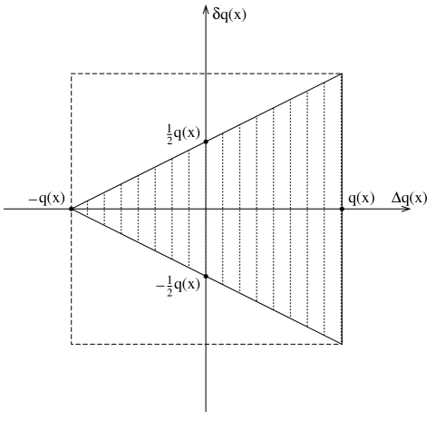
Figure 10: The Soffer bound on the leading-twist distributions [38] (note that there $\Delta_{T}{q}(x)$ was called $\delta{q}(x)$).

We shall see in Sec. 5.5 that the Soffer bound, like the other two – more obvious – inequalities (4.6.1a, LABEL:subsoffer0.2), is preserved by QCD evolution, as it should be.

4.7 Transverse motion of quarks

Let us now account for the transverse motion of quarks. This is necessary in semi-inclusive DIS, when one wants to study the $\mathchoice{\mbox{\boldmath$\displaystyle P$\unboldmath}}{\mbox{\boldmath$\textstyle P$\unboldmath}}{\mbox{\boldmath$\scriptstyle P$\unboldmath}}{\mbox{\boldmath$\scriptscriptstyle P$\unboldmath}}_{h\perp}$ distribution of the produced hadron. Therefore, in this section we shall prepare the field for later applications.

The quark momentum is now given by

$$k^{\mu}\simeq xP^{\mu}+k_{\perp}^{\mu}\,,$$ (4.7.1)

where we have retained $k_{\perp}^{\mu}$, which is zeroth order in $P^{+}$ and thus suppressed by one power of $P^{+}$ with respect to the longitudinal momentum.

At leading twist, again, only the vector, axial and tensor terms in (4.1.6) appear and eqs. (4.1.7b, LABEL:subdf2.3, LABEL:subdf2.5) become

$$\mathcal{V}^{\mu} = \,A_{1}\,P^{\mu}\,,$$ (4.7.2a)

$$\mathcal{A}^{\mu} = \lambda_{N}\,A_{2}\,P^{\mu}+\frac{1}{M}\,\widetilde{A}_{1}\,\mathchoice{\mbox{\boldmath$\displaystyle k$\unboldmath}}{\mbox{\boldmath$\textstyle k$\unboldmath}}{\mbox{\boldmath$\scriptstyle k$\unboldmath}}{\mbox{\boldmath$\scriptscriptstyle k$\unboldmath}}_{\perp}{\cdot}\mathchoice{\mbox{\boldmath$\displaystyle S$\unboldmath}}{\mbox{\boldmath$\textstyle S$\unboldmath}}{\mbox{\boldmath$\scriptstyle S$\unboldmath}}{\mbox{\boldmath$\scriptscriptstyle S$\unboldmath}}_{\perp}\,P^{\mu}\,,$$ (4.7.2b)

$$\mathcal{T}^{\mu\nu} = A_{3}\,P_{\vphantom{\perp}}^{[\mu}S_{\perp}^{\nu]}\,+\frac{\lambda_{N}}{M}\,\widetilde{A}_{2}\,P_{\vphantom{\perp}}^{[\mu}k_{\perp}^{\nu]}+\frac{1}{M^{2}}\,\widetilde{A}_{3}\,\mathchoice{\mbox{\boldmath$\displaystyle k$\unboldmath}}{\mbox{\boldmath$\textstyle k$\unboldmath}}{\mbox{\boldmath$\scriptstyle k$\unboldmath}}{\mbox{\boldmath$\scriptscriptstyle k$\unboldmath}}_{\perp}{\cdot}\mathchoice{\mbox{\boldmath$\displaystyle S$\unboldmath}}{\mbox{\boldmath$\textstyle S$\unboldmath}}{\mbox{\boldmath$\scriptstyle S$\unboldmath}}{\mbox{\boldmath$\scriptscriptstyle S$\unboldmath}}_{\perp}\,P_{\vphantom{\perp}}^{[\mu}k_{\perp}^{\nu]}\,,$$ (4.7.2c)

where we have defined new real functions $\widetilde{A}_{i}(k^{2},k{\cdot}P)$ (the tilde signals the presence of $\mathchoice{\mbox{\boldmath$\displaystyle k$\unboldmath}}{\mbox{\boldmath$\textstyle k$\unboldmath}}{\mbox{\boldmath$\scriptstyle k$\unboldmath}}{\mbox{\boldmath$\scriptscriptstyle k$\unboldmath}}_{\perp}$) and introduced powers of $M$, so that all coefficients have the same dimension. The quark–quark correlation matrix (4.1.6) then reads

$$\Phi(k,P,S) = \frac{1}{2}\left\{\rule[-7.3194pt]{0.0pt}{20.23602pt}A_{1}\,\not{P}+A_{2}\,\lambda_{N}\,\gamma_{5}\,\not{P}+A_{3}\,\not{P}\,\gamma_{5}\,\not{S}_{\perp}\right.$$ (4.7.3)

$$\qquad\hbox{}+\left.\frac{1}{M}\,\widetilde{A}_{1}\,\mathchoice{\mbox{\boldmath$\displaystyle k$\unboldmath}}{\mbox{\boldmath$\textstyle k$\unboldmath}}{\mbox{\boldmath$\scriptstyle k$\unboldmath}}{\mbox{\boldmath$\scriptscriptstyle k$\unboldmath}}_{\perp}{\cdot}\mathchoice{\mbox{\boldmath$\displaystyle S$\unboldmath}}{\mbox{\boldmath$\textstyle S$\unboldmath}}{\mbox{\boldmath$\scriptstyle S$\unboldmath}}{\mbox{\boldmath$\scriptscriptstyle S$\unboldmath}}_{\perp}\,\gamma_{5}\not{P}+\widetilde{A}_{2}\,\frac{\lambda_{N}}{M}\,\not{P}\,\gamma_{5}\,\not{k}_{\perp}\right.$$

$$\qquad\hbox{}+\left.\frac{1}{M^{2}}\,\widetilde{A}_{3}\,\mathchoice{\mbox{\boldmath$\displaystyle k$\unboldmath}}{\mbox{\boldmath$\textstyle k$\unboldmath}}{\mbox{\boldmath$\scriptstyle k$\unboldmath}}{\mbox{\boldmath$\scriptscriptstyle k$\unboldmath}}_{\perp}{\cdot}\mathchoice{\mbox{\boldmath$\displaystyle S$\unboldmath}}{\mbox{\boldmath$\textstyle S$\unboldmath}}{\mbox{\boldmath$\scriptstyle S$\unboldmath}}{\mbox{\boldmath$\scriptscriptstyle S$\unboldmath}}_{\perp}\,\not{P}\,\gamma_{5}\,\not{k}_{\perp}\right\}.$$

We can project out the $A_{i}$’s and $\widetilde{A}_{i}$’s, as we did in Sec. 4.2

$$\frac{1}{2P^{+}}\,\mathop{\text{Tr}}\nolimits(\gamma^{+}\Phi) = A_{1}\,,$$ (4.7.4a)

$$\frac{1}{2P^{+}}\,\mathop{\text{Tr}}\nolimits(\gamma^{+}\gamma_{5}\Phi) = \lambda_{N}\,A_{2}+\frac{1}{M}\,\mathchoice{\mbox{\boldmath$\displaystyle k$\unboldmath}}{\mbox{\boldmath$\textstyle k$\unboldmath}}{\mbox{\boldmath$\scriptstyle k$\unboldmath}}{\mbox{\boldmath$\scriptscriptstyle k$\unboldmath}}_{\perp}{\cdot}\mathchoice{\mbox{\boldmath$\displaystyle S$\unboldmath}}{\mbox{\boldmath$\textstyle S$\unboldmath}}{\mbox{\boldmath$\scriptstyle S$\unboldmath}}{\mbox{\boldmath$\scriptscriptstyle S$\unboldmath}}_{\perp}\,\widetilde{A}_{1}\,,$$ (4.7.4b)

$$\frac{1}{2P^{+}}\,\mathop{\text{Tr}}\nolimits(\text{i}\sigma^{i+}\gamma_{5}\Phi) = S_{\perp}^{i}\,A_{3}+\frac{\lambda_{N}}{M}\,k_{\perp}^{i}\,\widetilde{A}_{2}+\frac{1}{M^{2}}\,\mathchoice{\mbox{\boldmath$\displaystyle k$\unboldmath}}{\mbox{\boldmath$\textstyle k$\unboldmath}}{\mbox{\boldmath$\scriptstyle k$\unboldmath}}{\mbox{\boldmath$\scriptscriptstyle k$\unboldmath}}_{\perp}{\cdot}\mathchoice{\mbox{\boldmath$\displaystyle S$\unboldmath}}{\mbox{\boldmath$\textstyle S$\unboldmath}}{\mbox{\boldmath$\scriptstyle S$\unboldmath}}{\mbox{\boldmath$\scriptscriptstyle S$\unboldmath}}_{\perp}\,k_{\perp}^{i}\,\widetilde{A}_{3}\,.$$ (4.7.4c)

Let us rearrange the r.h.s. of the last expression in the following manner

$$S_{\perp}^{i}\,A_{3}+\frac{1}{M^{2}}\,\mathchoice{\mbox{\boldmath$\displaystyle k$\unboldmath}}{\mbox{\boldmath$\textstyle k$\unboldmath}}{\mbox{\boldmath$\scriptstyle k$\unboldmath}}{\mbox{\boldmath$\scriptscriptstyle k$\unboldmath}}_{\perp}{\cdot}\mathchoice{\mbox{\boldmath$\displaystyle S$\unboldmath}}{\mbox{\boldmath$\textstyle S$\unboldmath}}{\mbox{\boldmath$\scriptstyle S$\unboldmath}}{\mbox{\boldmath$\scriptscriptstyle S$\unboldmath}}_{\perp}\,k_{\perp}^{i}\,\widetilde{A}_{3} = S_{\perp}^{i}\left(A_{3}+\frac{\mathchoice{\mbox{\boldmath$\displaystyle k$\unboldmath}}{\mbox{\boldmath$\textstyle k$\unboldmath}}{\mbox{\boldmath$\scriptstyle k$\unboldmath}}{\mbox{\boldmath$\scriptscriptstyle k$\unboldmath}}_{\perp}^{2}}{2M^{2}}\,\widetilde{A}_{3}\right)$$ (4.7.5)

$$\hbox{}-\frac{1}{M^{2}}\left(k_{\perp}^{i}k_{\perp}^{j}+\frac{1}{2}\,\mathchoice{\mbox{\boldmath$\displaystyle k$\unboldmath}}{\mbox{\boldmath$\textstyle k$\unboldmath}}{\mbox{\boldmath$\scriptstyle k$\unboldmath}}{\mbox{\boldmath$\scriptscriptstyle k$\unboldmath}}_{\perp}^{2}\,g_{\perp}^{ij}\right)S_{\perp j}\,\widetilde{A}_{3}\,.\hskip 20.00003pt$$

If we integrate eqs. (4.7.4a–LABEL:subtm8) over $k$ with the constraint $x=k^{+}/P^{+}$, the terms proportional to $\widetilde{A}_{1}$, $\widetilde{A}_{2}$ and $\widetilde{A}_{3}$ in (4.7.4b, LABEL:subtm8) and (4.7.5) vanish. We are left with the three terms proportional to $A_{1}$, $A_{2}$ and to the combination $A_{3}+(\mathchoice{\mbox{\boldmath$\displaystyle k$\unboldmath}}{\mbox{\boldmath$\textstyle k$\unboldmath}}{\mbox{\boldmath$\scriptstyle k$\unboldmath}}{\mbox{\boldmath$\scriptscriptstyle k$\unboldmath}}_{\perp}^{2}/2M^{2})\,\widetilde{A}_{3}$, which give, upon integration, the three distribution functions $f(x)$, $\Delta{f}(x)$ and $\Delta_{T}{f}(x)$, respectively. The only difference from the previous case of no quark transverse momentum is that $\Delta_{T}{f}(x)$ is now related to $A_{3}+(\mathchoice{\mbox{\boldmath$\displaystyle k$\unboldmath}}{\mbox{\boldmath$\textstyle k$\unboldmath}}{\mbox{\boldmath$\scriptstyle k$\unboldmath}}{\mbox{\boldmath$\scriptscriptstyle k$\unboldmath}}_{\perp}^{2}/2M^{2})\,\widetilde{A}_{3}$ and not to $A_{3}$ alone

$$\Delta_{T}{f}(x)\equiv\int\!\frac{\d^{4}k}{(2\pi)^{4}}\left(A_{3}+\frac{\mathchoice{\mbox{\boldmath$\displaystyle k$\unboldmath}}{\mbox{\boldmath$\textstyle k$\unboldmath}}{\mbox{\boldmath$\scriptstyle k$\unboldmath}}{\mbox{\boldmath$\scriptscriptstyle k$\unboldmath}}_{\perp}^{2}}{2M^{2}}\,\widetilde{A}_{3}\right)\delta(x-k^{+}/P^{+})\,.$$ (4.7.6)

If we do not integrate over $\mathchoice{\mbox{\boldmath$\displaystyle k$\unboldmath}}{\mbox{\boldmath$\textstyle k$\unboldmath}}{\mbox{\boldmath$\scriptstyle k$\unboldmath}}{\mbox{\boldmath$\scriptscriptstyle k$\unboldmath}}_{\perp}$, we obtain six $\mathchoice{\mbox{\boldmath$\displaystyle k$\unboldmath}}{\mbox{\boldmath$\textstyle k$\unboldmath}}{\mbox{\boldmath$\scriptstyle k$\unboldmath}}{\mbox{\boldmath$\scriptscriptstyle k$\unboldmath}}_{\perp}$-dependent distribution functions. Three of them, which we call $f(x,\mathchoice{\mbox{\boldmath$\displaystyle k$\unboldmath}}{\mbox{\boldmath$\textstyle k$\unboldmath}}{\mbox{\boldmath$\scriptstyle k$\unboldmath}}{\mbox{\boldmath$\scriptscriptstyle k$\unboldmath}}_{\perp}^{2})$, $\Delta{f}(x,\mathchoice{\mbox{\boldmath$\displaystyle k$\unboldmath}}{\mbox{\boldmath$\textstyle k$\unboldmath}}{\mbox{\boldmath$\scriptstyle k$\unboldmath}}{\mbox{\boldmath$\scriptscriptstyle k$\unboldmath}}_{\perp}^{2})$ and $\Delta_{T}^{\prime}f(x,\mathchoice{\mbox{\boldmath$\displaystyle k$\unboldmath}}{\mbox{\boldmath$\textstyle k$\unboldmath}}{\mbox{\boldmath$\scriptstyle k$\unboldmath}}{\mbox{\boldmath$\scriptscriptstyle k$\unboldmath}}_{\perp}^{2})$, are such that $f(x)=\int\d^{2}\mathchoice{\mbox{\boldmath$\displaystyle k$\unboldmath}}{\mbox{\boldmath$\textstyle k$\unboldmath}}{\mbox{\boldmath$\scriptstyle k$\unboldmath}}{\mbox{\boldmath$\scriptscriptstyle k$\unboldmath}}_{\perp}f(x,\mathchoice{\mbox{\boldmath$\displaystyle k$\unboldmath}}{\mbox{\boldmath$\textstyle k$\unboldmath}}{\mbox{\boldmath$\scriptstyle k$\unboldmath}}{\mbox{\boldmath$\scriptscriptstyle k$\unboldmath}}_{\perp}^{2})$, etc. The other three are completely new and are related to the terms of the correlation matrix containing the $\widetilde{A}_{i}$’s. We shall adopt Mulders’ terminology for them [15, 16]. Introducing the notation

$$\Phi^{[\Gamma]} \equiv \frac{1}{2}\int\!\frac{\d{k}^{+}\,\d{k}^{-}}{(2\pi)^{4}}\,\mathop{\text{Tr}}\nolimits(\Gamma\,\Phi)\,\delta(k^{+}-xP^{+})$$ (4.7.7)

$$= \int\!\frac{\d\xi^{-}\,\d^{2}\mathchoice{\mbox{\boldmath$\displaystyle\xi$\unboldmath}}{\mbox{\boldmath$\textstyle\xi$\unboldmath}}{\mbox{\boldmath$\scriptstyle\xi$\unboldmath}}{\mbox{\boldmath$\scriptscriptstyle\xi$\unboldmath}}_{\perp}}{2(2\pi)^{3}}\e^{\text{i}(xP^{+}\xi^{-}-\mathchoice{\mbox{\boldmath$\displaystyle k$\unboldmath}}{\mbox{\boldmath$\textstyle k$\unboldmath}}{\mbox{\boldmath$\scriptstyle k$\unboldmath}}{\mbox{\boldmath$\scriptscriptstyle k$\unboldmath}}_{\perp}{\cdot}\mathchoice{\mbox{\boldmath$\displaystyle\xi$\unboldmath}}{\mbox{\boldmath$\textstyle\xi$\unboldmath}}{\mbox{\boldmath$\scriptstyle\xi$\unboldmath}}{\mbox{\boldmath$\scriptscriptstyle\xi$\unboldmath}}_{\perp})}\langle PS|\mathchoice{\makebox[0.0pt][l]{$\displaystyle\kern 2.08334pt\overline{\kern-2.43059pt\phantom{\psi}}$}}{\makebox[0.0pt][l]{$\textstyle\kern 2.08334pt\overline{\kern-2.43059pt\phantom{\psi}}$}}{\makebox[0.0pt][l]{$\scriptstyle\kern 1.45834pt\overline{\kern-1.7014pt\phantom{\psi}}$}}{\makebox[0.0pt][l]{$\scriptscriptstyle\kern 1.04167pt\overline{\kern-1.21529pt\phantom{\psi}}$}}\psi(0)\Gamma\psi(0,\xi^{-},\mathchoice{\mbox{\boldmath$\displaystyle\xi$\unboldmath}}{\mbox{\boldmath$\textstyle\xi$\unboldmath}}{\mbox{\boldmath$\scriptstyle\xi$\unboldmath}}{\mbox{\boldmath$\scriptscriptstyle\xi$\unboldmath}}_{\perp})|PS\rangle\,,\qquad$$

we have

$$\Phi^{[\gamma^{+}]} = \mathcal{P}_{q/N}(x,\mathchoice{\mbox{\boldmath$\displaystyle k$\unboldmath}}{\mbox{\boldmath$\textstyle k$\unboldmath}}{\mbox{\boldmath$\scriptstyle k$\unboldmath}}{\mbox{\boldmath$\scriptscriptstyle k$\unboldmath}}_{\perp})=f(x,\mathchoice{\mbox{\boldmath$\displaystyle k$\unboldmath}}{\mbox{\boldmath$\textstyle k$\unboldmath}}{\mbox{\boldmath$\scriptstyle k$\unboldmath}}{\mbox{\boldmath$\scriptscriptstyle k$\unboldmath}}_{\perp}^{2})\,,$$ (4.7.8a)

$$\Phi^{[\gamma^{+}\gamma_{5}]} = \mathcal{P}_{q/N}(x,\mathchoice{\mbox{\boldmath$\displaystyle k$\unboldmath}}{\mbox{\boldmath$\textstyle k$\unboldmath}}{\mbox{\boldmath$\scriptstyle k$\unboldmath}}{\mbox{\boldmath$\scriptscriptstyle k$\unboldmath}}_{\perp})\,\lambda(x,\mathchoice{\mbox{\boldmath$\displaystyle k$\unboldmath}}{\mbox{\boldmath$\textstyle k$\unboldmath}}{\mbox{\boldmath$\scriptstyle k$\unboldmath}}{\mbox{\boldmath$\scriptscriptstyle k$\unboldmath}}_{\perp})$$ (4.7.8b)

$$= \lambda_{N}\,\Delta{f}(x,\mathchoice{\mbox{\boldmath$\displaystyle k$\unboldmath}}{\mbox{\boldmath$\textstyle k$\unboldmath}}{\mbox{\boldmath$\scriptstyle k$\unboldmath}}{\mbox{\boldmath$\scriptscriptstyle k$\unboldmath}}_{\perp}^{2})+\frac{\mathchoice{\mbox{\boldmath$\displaystyle k$\unboldmath}}{\mbox{\boldmath$\textstyle k$\unboldmath}}{\mbox{\boldmath$\scriptstyle k$\unboldmath}}{\mbox{\boldmath$\scriptscriptstyle k$\unboldmath}}_{\perp}{\cdot}\mathchoice{\mbox{\boldmath$\displaystyle S$\unboldmath}}{\mbox{\boldmath$\textstyle S$\unboldmath}}{\mbox{\boldmath$\scriptstyle S$\unboldmath}}{\mbox{\boldmath$\scriptscriptstyle S$\unboldmath}}_{\perp}}{M}\,g_{1T}(x,\mathchoice{\mbox{\boldmath$\displaystyle k$\unboldmath}}{\mbox{\boldmath$\textstyle k$\unboldmath}}{\mbox{\boldmath$\scriptstyle k$\unboldmath}}{\mbox{\boldmath$\scriptscriptstyle k$\unboldmath}}_{\perp}^{2})\,,$$

$$\Phi^{[\text{i}\sigma^{i+}\gamma_{5}]} = \mathcal{P}_{q/N}(x,\mathchoice{\mbox{\boldmath$\displaystyle k$\unboldmath}}{\mbox{\boldmath$\textstyle k$\unboldmath}}{\mbox{\boldmath$\scriptstyle k$\unboldmath}}{\mbox{\boldmath$\scriptscriptstyle k$\unboldmath}}_{\perp})\,s_{\perp}^{i}(x,\mathchoice{\mbox{\boldmath$\displaystyle k$\unboldmath}}{\mbox{\boldmath$\textstyle k$\unboldmath}}{\mbox{\boldmath$\scriptstyle k$\unboldmath}}{\mbox{\boldmath$\scriptscriptstyle k$\unboldmath}}_{\perp})$$ (4.7.8c)

$$= S_{\perp}^{i}\,\Delta_{T}^{\prime}f(x,\mathchoice{\mbox{\boldmath$\displaystyle k$\unboldmath}}{\mbox{\boldmath$\textstyle k$\unboldmath}}{\mbox{\boldmath$\scriptstyle k$\unboldmath}}{\mbox{\boldmath$\scriptscriptstyle k$\unboldmath}}_{\perp}^{2})+\frac{\lambda_{N}}{M}\,k_{\perp}^{i}\,h_{1L}^{\perp}(x,\mathchoice{\mbox{\boldmath$\displaystyle k$\unboldmath}}{\mbox{\boldmath$\textstyle k$\unboldmath}}{\mbox{\boldmath$\scriptstyle k$\unboldmath}}{\mbox{\boldmath$\scriptscriptstyle k$\unboldmath}}_{\perp}^{2})$$

$$\hbox{}-\frac{1}{M^{2}}\left(k_{\perp}^{i}k_{\perp}^{j}+\frac{1}{2}\,\mathchoice{\mbox{\boldmath$\displaystyle k$\unboldmath}}{\mbox{\boldmath$\textstyle k$\unboldmath}}{\mbox{\boldmath$\scriptstyle k$\unboldmath}}{\mbox{\boldmath$\scriptscriptstyle k$\unboldmath}}_{\perp}^{2}\,g_{\perp}^{ij}\right)S_{\perp j}\,h_{1T}^{\perp}(x,\mathchoice{\mbox{\boldmath$\displaystyle k$\unboldmath}}{\mbox{\boldmath$\textstyle k$\unboldmath}}{\mbox{\boldmath$\scriptstyle k$\unboldmath}}{\mbox{\boldmath$\scriptscriptstyle k$\unboldmath}}_{\perp}^{2})\,,$$

where $\mathcal{P}_{q/N}(x,\mathchoice{\mbox{\boldmath$\displaystyle k$\unboldmath}}{\mbox{\boldmath$\textstyle k$\unboldmath}}{\mbox{\boldmath$\scriptstyle k$\unboldmath}}{\mbox{\boldmath$\scriptscriptstyle k$\unboldmath}}_{\perp})$ is the probability of finding a quark with longitudinal momentum fraction $x$ and transverse momentum $\mathchoice{\mbox{\boldmath$\displaystyle k$\unboldmath}}{\mbox{\boldmath$\textstyle k$\unboldmath}}{\mbox{\boldmath$\scriptstyle k$\unboldmath}}{\mbox{\boldmath$\scriptscriptstyle k$\unboldmath}}_{\perp}$, and $\lambda(x,\mathchoice{\mbox{\boldmath$\displaystyle k$\unboldmath}}{\mbox{\boldmath$\textstyle k$\unboldmath}}{\mbox{\boldmath$\scriptstyle k$\unboldmath}}{\mbox{\boldmath$\scriptscriptstyle k$\unboldmath}}_{\perp})$, $\mathchoice{\mbox{\boldmath$\displaystyle s$\unboldmath}}{\mbox{\boldmath$\textstyle s$\unboldmath}}{\mbox{\boldmath$\scriptstyle s$\unboldmath}}{\mbox{\boldmath$\scriptscriptstyle s$\unboldmath}}_{\perp}(x,\mathchoice{\mbox{\boldmath$\displaystyle k$\unboldmath}}{\mbox{\boldmath$\textstyle k$\unboldmath}}{\mbox{\boldmath$\scriptstyle k$\unboldmath}}{\mbox{\boldmath$\scriptscriptstyle k$\unboldmath}}_{\perp})$ are the quark helicity and transverse spin densities, respectively. The spin density matrix of quarks now reads

$$\rho_{\lambda\lambda^{\prime}}=\frac{1}{2}\left(\begin{array}[]{cc}1+\lambda(x,\mathchoice{\mbox{\boldmath$\displaystyle k$\unboldmath}}{\mbox{\boldmath$\textstyle k$\unboldmath}}{\mbox{\boldmath$\scriptstyle k$\unboldmath}}{\mbox{\boldmath$\scriptscriptstyle k$\unboldmath}}_{\perp})&s_{x}(x,\mathchoice{\mbox{\boldmath$\displaystyle k$\unboldmath}}{\mbox{\boldmath$\textstyle k$\unboldmath}}{\mbox{\boldmath$\scriptstyle k$\unboldmath}}{\mbox{\boldmath$\scriptscriptstyle k$\unboldmath}}_{\perp})-\text{i}s_{y}(x,\mathchoice{\mbox{\boldmath$\displaystyle k$\unboldmath}}{\mbox{\boldmath$\textstyle k$\unboldmath}}{\mbox{\boldmath$\scriptstyle k$\unboldmath}}{\mbox{\boldmath$\scriptscriptstyle k$\unboldmath}}_{\perp})\\ s_{x}(x,\mathchoice{\mbox{\boldmath$\displaystyle k$\unboldmath}}{\mbox{\boldmath$\textstyle k$\unboldmath}}{\mbox{\boldmath$\scriptstyle k$\unboldmath}}{\mbox{\boldmath$\scriptscriptstyle k$\unboldmath}}_{\perp})+\text{i}s_{y}(x,\mathchoice{\mbox{\boldmath$\displaystyle k$\unboldmath}}{\mbox{\boldmath$\textstyle k$\unboldmath}}{\mbox{\boldmath$\scriptstyle k$\unboldmath}}{\mbox{\boldmath$\scriptscriptstyle k$\unboldmath}}_{\perp})&1-\lambda(x,\mathchoice{\mbox{\boldmath$\displaystyle k$\unboldmath}}{\mbox{\boldmath$\textstyle k$\unboldmath}}{\mbox{\boldmath$\scriptstyle k$\unboldmath}}{\mbox{\boldmath$\scriptscriptstyle k$\unboldmath}}_{\perp})\end{array}\right),$$ (4.7.9)

and its entries incorporate the six distributions listed above, according to eqs. (4.7.8a–4.7.8b).

Let us now try to understand the partonic content of the $\mathchoice{\mbox{\boldmath$\displaystyle k$\unboldmath}}{\mbox{\boldmath$\textstyle k$\unboldmath}}{\mbox{\boldmath$\scriptstyle k$\unboldmath}}{\mbox{\boldmath$\scriptscriptstyle k$\unboldmath}}_{\perp}$-dependent distributions. If the target nucleon is unpolarised, the only measurable quantity is $f(x,\mathchoice{\mbox{\boldmath$\displaystyle k$\unboldmath}}{\mbox{\boldmath$\textstyle k$\unboldmath}}{\mbox{\boldmath$\scriptstyle k$\unboldmath}}{\mbox{\boldmath$\scriptscriptstyle k$\unboldmath}}_{\perp}^{2})$, which coincides with $\mathcal{P}_{q}(x,\mathchoice{\mbox{\boldmath$\displaystyle k$\unboldmath}}{\mbox{\boldmath$\textstyle k$\unboldmath}}{\mbox{\boldmath$\scriptstyle k$\unboldmath}}{\mbox{\boldmath$\scriptscriptstyle k$\unboldmath}}_{\perp})$, the number density of quarks with longitudinal momentum fraction $x$ and transverse momentum squared $\mathchoice{\mbox{\boldmath$\displaystyle k$\unboldmath}}{\mbox{\boldmath$\textstyle k$\unboldmath}}{\mbox{\boldmath$\scriptstyle k$\unboldmath}}{\mbox{\boldmath$\scriptscriptstyle k$\unboldmath}}_{\perp}^{2}$.

If the target nucleon is transversely polarised, there is some probability of finding the quarks transversely polarised along the same direction as the nucleon, along a different direction, or longitudinally polarised. This variety of situations is allowed by the presence of $\mathchoice{\mbox{\boldmath$\displaystyle k$\unboldmath}}{\mbox{\boldmath$\textstyle k$\unboldmath}}{\mbox{\boldmath$\scriptstyle k$\unboldmath}}{\mbox{\boldmath$\scriptscriptstyle k$\unboldmath}}_{\perp}$. Integrating over $\mathchoice{\mbox{\boldmath$\displaystyle k$\unboldmath}}{\mbox{\boldmath$\textstyle k$\unboldmath}}{\mbox{\boldmath$\scriptstyle k$\unboldmath}}{\mbox{\boldmath$\scriptscriptstyle k$\unboldmath}}_{\perp}$, the transverse polarisation asymmetry of quarks along a different direction with respect to the nucleon polarisation, and the longitudinal polarisation asymmetry of quarks in a transversely polarised nucleon disappear: only the case $\mathchoice{\mbox{\boldmath$\displaystyle s$\unboldmath}}{\mbox{\boldmath$\textstyle s$\unboldmath}}{\mbox{\boldmath$\scriptstyle s$\unboldmath}}{\mbox{\boldmath$\scriptscriptstyle s$\unboldmath}}_{\perp}\parallel\mathchoice{\mbox{\boldmath$\displaystyle S$\unboldmath}}{\mbox{\boldmath$\textstyle S$\unboldmath}}{\mbox{\boldmath$\scriptstyle S$\unboldmath}}{\mbox{\boldmath$\scriptscriptstyle S$\unboldmath}}_{\perp}$ survives.

Referring to Fig. 11 for the geometry in the azimuthal plane and using the following parametrisations for the vectors at hand (we assume full polarisation of the nucleon):

$$\mathchoice{\mbox{\boldmath$\displaystyle k$\unboldmath}}{\mbox{\boldmath$\textstyle k$\unboldmath}}{\mbox{\boldmath$\scriptstyle k$\unboldmath}}{\mbox{\boldmath$\scriptscriptstyle k$\unboldmath}}_{\perp} = (|\mathchoice{\mbox{\boldmath$\displaystyle k$\unboldmath}}{\mbox{\boldmath$\textstyle k$\unboldmath}}{\mbox{\boldmath$\scriptstyle k$\unboldmath}}{\mbox{\boldmath$\scriptscriptstyle k$\unboldmath}}_{\perp}|\,\cos\phi_{k},\,-|\mathchoice{\mbox{\boldmath$\displaystyle k$\unboldmath}}{\mbox{\boldmath$\textstyle k$\unboldmath}}{\mbox{\boldmath$\scriptstyle k$\unboldmath}}{\mbox{\boldmath$\scriptscriptstyle k$\unboldmath}}_{\perp}|\,\sin\phi_{k})\,,$$ (4.7.10)

$$\mathchoice{\mbox{\boldmath$\displaystyle S$\unboldmath}}{\mbox{\boldmath$\textstyle S$\unboldmath}}{\mbox{\boldmath$\scriptstyle S$\unboldmath}}{\mbox{\boldmath$\scriptscriptstyle S$\unboldmath}}_{\perp} = (\cos\phi_{S},\,-\sin\phi_{S})\,,$$ (4.7.11)

$$\mathchoice{\mbox{\boldmath$\displaystyle s$\unboldmath}}{\mbox{\boldmath$\textstyle s$\unboldmath}}{\mbox{\boldmath$\scriptstyle s$\unboldmath}}{\mbox{\boldmath$\scriptscriptstyle s$\unboldmath}}_{\perp} = (|\mathchoice{\mbox{\boldmath$\displaystyle s$\unboldmath}}{\mbox{\boldmath$\textstyle s$\unboldmath}}{\mbox{\boldmath$\scriptstyle s$\unboldmath}}{\mbox{\boldmath$\scriptscriptstyle s$\unboldmath}}_{\perp}|\,\cos\phi_{s},\,-|\mathchoice{\mbox{\boldmath$\displaystyle s$\unboldmath}}{\mbox{\boldmath$\textstyle s$\unboldmath}}{\mbox{\boldmath$\scriptstyle s$\unboldmath}}{\mbox{\boldmath$\scriptscriptstyle s$\unboldmath}}_{\perp}|\,\sin\phi_{s})\,,$$ (4.7.12)

we find for the $\mathchoice{\mbox{\boldmath$\displaystyle k$\unboldmath}}{\mbox{\boldmath$\textstyle k$\unboldmath}}{\mbox{\boldmath$\scriptstyle k$\unboldmath}}{\mbox{\boldmath$\scriptscriptstyle k$\unboldmath}}_{\perp}$-dependent transverse polarisation distributions of quarks in a transversely polarised nucleon (${\pm}$ denote, as usual, longitudinal polarisation whereas $\uparrow\downarrow$ denote transverse polarisation)

$$\mathcal{P}_{q\uparrow/N\uparrow}(x,\mathchoice{\mbox{\boldmath$\displaystyle k$\unboldmath}}{\mbox{\boldmath$\textstyle k$\unboldmath}}{\mbox{\boldmath$\scriptstyle k$\unboldmath}}{\mbox{\boldmath$\scriptscriptstyle k$\unboldmath}}_{\perp})-\mathcal{P}_{q\downarrow/N\uparrow}(x,\mathchoice{\mbox{\boldmath$\displaystyle k$\unboldmath}}{\mbox{\boldmath$\textstyle k$\unboldmath}}{\mbox{\boldmath$\scriptstyle k$\unboldmath}}{\mbox{\boldmath$\scriptscriptstyle k$\unboldmath}}_{\perp}) = \cos(\phi_{S}-\phi_{s})\,\Delta_{T}^{\prime}f(x,\mathchoice{\mbox{\boldmath$\displaystyle k$\unboldmath}}{\mbox{\boldmath$\textstyle k$\unboldmath}}{\mbox{\boldmath$\scriptstyle k$\unboldmath}}{\mbox{\boldmath$\scriptscriptstyle k$\unboldmath}}_{\perp}^{2})$$ (4.7.13a)

$$\hbox{}+\frac{\mathchoice{\mbox{\boldmath$\displaystyle k$\unboldmath}}{\mbox{\boldmath$\textstyle k$\unboldmath}}{\mbox{\boldmath$\scriptstyle k$\unboldmath}}{\mbox{\boldmath$\scriptscriptstyle k$\unboldmath}}_{\perp}^{2}}{2M^{2}}\,\cos(2\phi_{k}-\phi_{S}-\phi_{s})\,h_{1T}^{\perp}(x,\mathchoice{\mbox{\boldmath$\displaystyle k$\unboldmath}}{\mbox{\boldmath$\textstyle k$\unboldmath}}{\mbox{\boldmath$\scriptstyle k$\unboldmath}}{\mbox{\boldmath$\scriptscriptstyle k$\unboldmath}}_{\perp}^{2})\,,\qquad$$

and for the longitudinal polarisation distribution of quarks in a transversely polarised nucleon

$$\mathcal{P}_{q+/N\uparrow}(x,\mathchoice{\mbox{\boldmath$\displaystyle k$\unboldmath}}{\mbox{\boldmath$\textstyle k$\unboldmath}}{\mbox{\boldmath$\scriptstyle k$\unboldmath}}{\mbox{\boldmath$\scriptscriptstyle k$\unboldmath}}_{\perp})-\mathcal{P}_{q-/N\uparrow}(x,\mathchoice{\mbox{\boldmath$\displaystyle k$\unboldmath}}{\mbox{\boldmath$\textstyle k$\unboldmath}}{\mbox{\boldmath$\scriptstyle k$\unboldmath}}{\mbox{\boldmath$\scriptscriptstyle k$\unboldmath}}_{\perp})=\frac{|\mathchoice{\mbox{\boldmath$\displaystyle k$\unboldmath}}{\mbox{\boldmath$\textstyle k$\unboldmath}}{\mbox{\boldmath$\scriptstyle k$\unboldmath}}{\mbox{\boldmath$\scriptscriptstyle k$\unboldmath}}_{\perp}|}{M}\,\cos(\phi_{S}-\phi_{k})\,g_{1T}(x,\mathchoice{\mbox{\boldmath$\displaystyle k$\unboldmath}}{\mbox{\boldmath$\textstyle k$\unboldmath}}{\mbox{\boldmath$\scriptstyle k$\unboldmath}}{\mbox{\boldmath$\scriptscriptstyle k$\unboldmath}}_{\perp}^{2})\,.$$ (4.7.13b)

Figure 11: Our definition of the azimuthal angles in the plane orthogonal to the $\gamma^{*}N$ axis. The photon momentum, which is directed along the positive $z$ axis, points inwards. For our choice of the axes see Fig. 5.

Due to transverse motion, quarks can also be transversely polarised in a longitudinally polarised nucleon. Their polarisation asymmetry is

$$\mathcal{P}_{q\uparrow/N+}(x,\mathchoice{\mbox{\boldmath$\displaystyle k$\unboldmath}}{\mbox{\boldmath$\textstyle k$\unboldmath}}{\mbox{\boldmath$\scriptstyle k$\unboldmath}}{\mbox{\boldmath$\scriptscriptstyle k$\unboldmath}}_{\perp})-\mathcal{P}_{q\downarrow/N+}(x,\mathchoice{\mbox{\boldmath$\displaystyle k$\unboldmath}}{\mbox{\boldmath$\textstyle k$\unboldmath}}{\mbox{\boldmath$\scriptstyle k$\unboldmath}}{\mbox{\boldmath$\scriptscriptstyle k$\unboldmath}}_{\perp})=\frac{|\mathchoice{\mbox{\boldmath$\displaystyle k$\unboldmath}}{\mbox{\boldmath$\textstyle k$\unboldmath}}{\mbox{\boldmath$\scriptstyle k$\unboldmath}}{\mbox{\boldmath$\scriptscriptstyle k$\unboldmath}}_{\perp}|}{M}\,\cos(\phi_{k}-\phi_{s})\,h_{1L}^{\perp}(x,\mathchoice{\mbox{\boldmath$\displaystyle k$\unboldmath}}{\mbox{\boldmath$\textstyle k$\unboldmath}}{\mbox{\boldmath$\scriptstyle k$\unboldmath}}{\mbox{\boldmath$\scriptscriptstyle k$\unboldmath}}_{\perp}^{2})\,.$$ (4.7.13c)

As we shall see in Sec. 6.5, the $\mathchoice{\mbox{\boldmath$\displaystyle k$\unboldmath}}{\mbox{\boldmath$\textstyle k$\unboldmath}}{\mbox{\boldmath$\scriptstyle k$\unboldmath}}{\mbox{\boldmath$\scriptscriptstyle k$\unboldmath}}_{\perp}$-dependent distribution function $h_{1L}^{\perp}$ plays a rôle in the azimuthal asymmetries of semi-inclusive leptoproduction.

4.8 $T$-odd distributions

Relaxing the time-reversal invariance condition (4.1.4c) – we postpone the discussion of the physical relevance of this until the end of this subsection – two additional terms in the vector and tensor components of $\Phi$ arise

$$\mathcal{V}^{\mu} =\dots+\frac{1}{M}\,A_{1}^{\prime}\,\varepsilon^{\mu\nu\rho\sigma}\,P_{\nu}k_{\perp\rho}S_{\perp\sigma}\,,$$ (4.1.7b^′′)

$$\mathcal{T}^{\mu\nu} =\dots+\frac{1}{M}\,A_{2}^{\prime}\,\varepsilon^{\mu\nu\rho\sigma}\,P_{\rho}k_{\perp\sigma}\,,$$ (4.1.7e^′′)

which give rise to two $\mathchoice{\mbox{\boldmath$\displaystyle k$\unboldmath}}{\mbox{\boldmath$\textstyle k$\unboldmath}}{\mbox{\boldmath$\scriptstyle k$\unboldmath}}{\mbox{\boldmath$\scriptscriptstyle k$\unboldmath}}_{\perp}$-dependent $T$-odd distribution functions, $f_{1T}^{\perp}$ and $h_{1}^{\perp}$

$$\Phi^{[\gamma^{+}]} = \dots-\frac{\varepsilon_{\perp}^{ij}k_{\perp i}S_{\perp j}}{M}\,f_{1T}^{\perp}(x,\mathchoice{\mbox{\boldmath$\displaystyle k$\unboldmath}}{\mbox{\boldmath$\textstyle k$\unboldmath}}{\mbox{\boldmath$\scriptstyle k$\unboldmath}}{\mbox{\boldmath$\scriptscriptstyle k$\unboldmath}}_{\perp}^{2})\,,$$ (4.8.1a)

$$\Phi^{[\text{i}\sigma^{i+}\gamma_{5}]} = \dots-\frac{\varepsilon_{\perp}^{ij}k_{\perp j}}{M}\,h_{1}^{\perp}(x,\mathchoice{\mbox{\boldmath$\displaystyle k$\unboldmath}}{\mbox{\boldmath$\textstyle k$\unboldmath}}{\mbox{\boldmath$\scriptstyle k$\unboldmath}}{\mbox{\boldmath$\scriptscriptstyle k$\unboldmath}}_{\perp}^{2})\,.$$ (4.8.1b)

Let us see the partonic interpretation of the new distributions. The first of them, $f_{1T}^{\perp}$, is related to the number density of unpolarised quarks in a transversely polarised nucleon. More precisely, it is given by

$$\mathcal{P}_{q/N\uparrow}(x,\mathchoice{\mbox{\boldmath$\displaystyle k$\unboldmath}}{\mbox{\boldmath$\textstyle k$\unboldmath}}{\mbox{\boldmath$\scriptstyle k$\unboldmath}}{\mbox{\boldmath$\scriptscriptstyle k$\unboldmath}}_{\perp})-\mathcal{P}_{q/N\downarrow}(x,\mathchoice{\mbox{\boldmath$\displaystyle k$\unboldmath}}{\mbox{\boldmath$\textstyle k$\unboldmath}}{\mbox{\boldmath$\scriptstyle k$\unboldmath}}{\mbox{\boldmath$\scriptscriptstyle k$\unboldmath}}_{\perp}) = \mathcal{P}_{q/N\uparrow}(x,\mathchoice{\mbox{\boldmath$\displaystyle k$\unboldmath}}{\mbox{\boldmath$\textstyle k$\unboldmath}}{\mbox{\boldmath$\scriptstyle k$\unboldmath}}{\mbox{\boldmath$\scriptscriptstyle k$\unboldmath}}_{\perp})-\mathcal{P}_{q/N\uparrow}(x,-\mathchoice{\mbox{\boldmath$\displaystyle k$\unboldmath}}{\mbox{\boldmath$\textstyle k$\unboldmath}}{\mbox{\boldmath$\scriptstyle k$\unboldmath}}{\mbox{\boldmath$\scriptscriptstyle k$\unboldmath}}_{\perp})$$ (4.8.2a)

$$= -2\frac{|\mathchoice{\mbox{\boldmath$\displaystyle k$\unboldmath}}{\mbox{\boldmath$\textstyle k$\unboldmath}}{\mbox{\boldmath$\scriptstyle k$\unboldmath}}{\mbox{\boldmath$\scriptscriptstyle k$\unboldmath}}_{\perp}|}{M}\,\sin(\phi_{k}-\phi_{S})\,f_{1T}^{\perp}(x,\mathchoice{\mbox{\boldmath$\displaystyle k$\unboldmath}}{\mbox{\boldmath$\textstyle k$\unboldmath}}{\mbox{\boldmath$\scriptstyle k$\unboldmath}}{\mbox{\boldmath$\scriptscriptstyle k$\unboldmath}}_{\perp}^{2})\,.\qquad$$

The other $$T h_{1}^{\perp}$$-odd distribution, , measures quark transverse polarisation in an unpolarised hadron [16] and is defined via

$$\mathcal{P}_{q\uparrow/N}(x,\mathchoice{\mbox{\boldmath$\displaystyle k$\unboldmath}}{\mbox{\boldmath$\textstyle k$\unboldmath}}{\mbox{\boldmath$\scriptstyle k$\unboldmath}}{\mbox{\boldmath$\scriptscriptstyle k$\unboldmath}}_{\perp})-\mathcal{P}_{q\downarrow/N}(x,\mathchoice{\mbox{\boldmath$\displaystyle k$\unboldmath}}{\mbox{\boldmath$\textstyle k$\unboldmath}}{\mbox{\boldmath$\scriptstyle k$\unboldmath}}{\mbox{\boldmath$\scriptscriptstyle k$\unboldmath}}_{\perp})=-\frac{|\mathchoice{\mbox{\boldmath$\displaystyle k$\unboldmath}}{\mbox{\boldmath$\textstyle k$\unboldmath}}{\mbox{\boldmath$\scriptstyle k$\unboldmath}}{\mbox{\boldmath$\scriptscriptstyle k$\unboldmath}}_{\perp}|}{M}\,\sin(\phi_{k}-\phi_{s})\,h_{1}^{\perp}(x,\mathchoice{\mbox{\boldmath$\displaystyle k$\unboldmath}}{\mbox{\boldmath$\textstyle k$\unboldmath}}{\mbox{\boldmath$\scriptstyle k$\unboldmath}}{\mbox{\boldmath$\scriptscriptstyle k$\unboldmath}}_{\perp}^{2})\,.$$ (4.8.2b)

We shall encounter again these distributions in the analysis of hadron production (Sec. 7.4). For later convenience we define two quantities $\Delta_{0}^{T}{f}$ and $\Delta_{T}^{0}{f}$, related to $f_{1T}^{\perp}$ and $h_{1}^{\perp}$, respectively, by (for the notation see Sec. 1.2)

$$\Delta_{0}^{T}f(x,\mathchoice{\mbox{\boldmath$\displaystyle k$\unboldmath}}{\mbox{\boldmath$\textstyle k$\unboldmath}}{\mbox{\boldmath$\scriptstyle k$\unboldmath}}{\mbox{\boldmath$\scriptscriptstyle k$\unboldmath}}_{\perp}^{2}) \equiv -2\frac{|\mathchoice{\mbox{\boldmath$\displaystyle k$\unboldmath}}{\mbox{\boldmath$\textstyle k$\unboldmath}}{\mbox{\boldmath$\scriptstyle k$\unboldmath}}{\mbox{\boldmath$\scriptscriptstyle k$\unboldmath}}_{\perp}|}{M}\,f_{1T}^{\perp}(x,\mathchoice{\mbox{\boldmath$\displaystyle k$\unboldmath}}{\mbox{\boldmath$\textstyle k$\unboldmath}}{\mbox{\boldmath$\scriptstyle k$\unboldmath}}{\mbox{\boldmath$\scriptscriptstyle k$\unboldmath}}_{\perp}^{2})\,,$$ (4.8.3a)

$$\Delta_{T}^{0}f(x,\mathchoice{\mbox{\boldmath$\displaystyle k$\unboldmath}}{\mbox{\boldmath$\textstyle k$\unboldmath}}{\mbox{\boldmath$\scriptstyle k$\unboldmath}}{\mbox{\boldmath$\scriptscriptstyle k$\unboldmath}}_{\perp}^{2}) \equiv -\,\frac{|\mathchoice{\mbox{\boldmath$\displaystyle k$\unboldmath}}{\mbox{\boldmath$\textstyle k$\unboldmath}}{\mbox{\boldmath$\scriptstyle k$\unboldmath}}{\mbox{\boldmath$\scriptscriptstyle k$\unboldmath}}_{\perp}|}{M}\,h_{1}^{\perp}(x,\mathchoice{\mbox{\boldmath$\displaystyle k$\unboldmath}}{\mbox{\boldmath$\textstyle k$\unboldmath}}{\mbox{\boldmath$\scriptstyle k$\unboldmath}}{\mbox{\boldmath$\scriptscriptstyle k$\unboldmath}}_{\perp}^{2})\,.$$ (4.8.3b)

It is now time to comment on the physical meaning of the quantities we have introduced in this section. One may legitimately wonder whether $T$-odd quark distributions, such as $f_{1T}^{\perp}$ and $h_{1}^{\perp}$ that violate the time-reversal condition (4.1.4c) make any sense at all. In order to justify the existence of $T$-odd distribution functions, their proponents [39] advocate initial-state effects, which prevent implementation of time-reversal invariance by naïvely imposing the condition (4.1.4c). The idea, similar to that which leads to admitting $T$-odd fragmentation functions as a result of final-state effects (see Sec. 6.4), is that the colliding particles interact strongly with non-trivial relative phases. As a consequence, time reversal no longer implies the constraint (4.1.4c). If hadronic interactions in the initial state are crucial to explain the existence of $f_{1T}^{\perp}$ and $h_{1}^{\perp}$, these distributions should only be observable in reactions involving two initial hadrons (Drell–Yan processes, hadron production in proton–proton collisions etc.). This mechanism is known as the Sivers effect [40, 41]. Clearly, it should be absent in leptoproduction.

A different way of looking at the $T$-odd distributions has been proposed in [42, 43, 44]. By relying on a general argument using time reversal, originally due to Wigner and recently revisited by Weinberg [45], the authors of [44] show that time reversal does not necessarily forbid $f_{1T}^{\perp}$ and $h_{1}^{\perp}$. In particular, an explicit realisation of Weinberg’s mechanism, based on chiral Lagrangians, shows that $f_{1T}^{\perp}$ and $h_{1}^{\perp}$ may emerge from the time-reversal preserving chiral dynamics of quarks in the nucleon, with no need for initial-state interaction effects. If this idea is correct, the $T$-odd distributions should also be observable in semi-inclusive leptoproduction. A conclusive statement on the matter will only be made by experiments.

4.9 Twist-three distributions

At twist 3 the quark–quark correlation matrix, integrated over $k$, has the structure [14]

$$\Phi(x)=\dots+\frac{M}{2}\left\{e(x)+g_{T}(x)\,\gamma_{5}\,\not{S}_{\perp}+\frac{\lambda_{N}}{2}\,h_{L}(x)\,\gamma_{5}\left[\not{p},\not{n}\right]\right\},$$ (4.9.1)

where the dots represent the twist-two contribution, eq. (4.2.8), and $p$, $n$ are the Sudakov vectors (see Appendix A). Three more distributions appear in (4.9.1): $e(x)$, $g_{T}(x)$ and $h_{L}(x)$. We already encountered $g_{T}(x)$, which is the twist-three partner of $\Delta{f}(x)$:

$$\int\!\frac{\d\tau}{2\pi}\,\e^{\text{i}\tau x}\,\langle PS|\mathchoice{\makebox[0.0pt][l]{$\displaystyle\kern 2.08334pt\overline{\kern-2.43059pt\phantom{\psi}}$}}{\makebox[0.0pt][l]{$\textstyle\kern 2.08334pt\overline{\kern-2.43059pt\phantom{\psi}}$}}{\makebox[0.0pt][l]{$\scriptstyle\kern 1.45834pt\overline{\kern-1.7014pt\phantom{\psi}}$}}{\makebox[0.0pt][l]{$\scriptscriptstyle\kern 1.04167pt\overline{\kern-1.21529pt\phantom{\psi}}$}}\psi(0)\gamma^{\mu}\gamma_{5}\psi(\tau n)|PS\rangle = 2\lambda_{N}\,\Delta{f}(x)\,p^{\mu}+2M\,g_{T}(x)\,S_{\perp}^{\mu}$$ (4.9.2a)

$$\hbox{}+\text{twist-4 terms}\,.$$

Analogously, $$h_{L}(x) \Delta_{T}{f}(x)$$ is the twist-three partner of and appears in the tensor term of the quark–quark correlation matrix:

$$\int\!\frac{\d\tau}{2\pi}\,\e^{\text{i}\tau x}\,\langle PS|\mathchoice{\makebox[0.0pt][l]{$\displaystyle\kern 2.08334pt\overline{\kern-2.43059pt\phantom{\psi}}$}}{\makebox[0.0pt][l]{$\textstyle\kern 2.08334pt\overline{\kern-2.43059pt\phantom{\psi}}$}}{\makebox[0.0pt][l]{$\scriptstyle\kern 1.45834pt\overline{\kern-1.7014pt\phantom{\psi}}$}}{\makebox[0.0pt][l]{$\scriptscriptstyle\kern 1.04167pt\overline{\kern-1.21529pt\phantom{\psi}}$}}\psi(0)\text{i}\sigma^{\mu\nu}\gamma_{5}\psi(\tau n)|PS\rangle = 2\Delta_{T}{f}(x)\,p_{\vphantom{\perp}}^{[\mu}S_{\perp}^{\nu]}+2M\,h_{L}(x)\,p^{[\mu}n^{\nu]}$$ (4.9.2b)

$$\hbox{}+\text{twist-4 terms.}$$

The third distribution, $$e(x)$$, has no counterpart at leading twist. It appears in the expansion of the scalar field bilinear:

$$\int\!\frac{\d\tau}{2\pi}\,\e^{\text{i}\tau x}\,\langle PS|\mathchoice{\makebox[0.0pt][l]{$\displaystyle\kern 2.08334pt\overline{\kern-2.43059pt\phantom{\psi}}$}}{\makebox[0.0pt][l]{$\textstyle\kern 2.08334pt\overline{\kern-2.43059pt\phantom{\psi}}$}}{\makebox[0.0pt][l]{$\scriptstyle\kern 1.45834pt\overline{\kern-1.7014pt\phantom{\psi}}$}}{\makebox[0.0pt][l]{$\scriptscriptstyle\kern 1.04167pt\overline{\kern-1.21529pt\phantom{\psi}}$}}\psi(0)\psi(\tau n)|PS\rangle=2M\,e(x)+\;\text{twist-4 terms.}$$ (4.9.2c)

The higher-twist distributions do not admit any probabilistic interpretation. To see this, consider for instance $g_{T}(x)$. Upon separation of $\psi$ into good and bad components, it turns out to be

$$g_{T}(x) = \frac{P^{+}}{M}\int\!\frac{\d\xi^{-}}{4\pi}\e^{\text{i}xP^{+}\xi^{-}}\langle PS|\psi_{(+)}^{\dagger}(0)\gamma^{0}\gamma^{1}\gamma_{5}\psi_{(-)}(0,\xi^{-},\mathchoice{\mbox{\boldmath$\displaystyle 0$\unboldmath}}{\mbox{\boldmath$\textstyle 0$\unboldmath}}{\mbox{\boldmath$\scriptstyle 0$\unboldmath}}{\mbox{\boldmath$\scriptscriptstyle 0$\unboldmath}}_{\perp})$$ (4.9.3)

$$\hskip 90.00014pt\hbox{}-\psi_{(-)}^{\dagger}(0)\gamma^{0}\gamma^{1}\gamma_{5}\psi_{(+)}(0,\xi^{-},\mathchoice{\mbox{\boldmath$\displaystyle 0$\unboldmath}}{\mbox{\boldmath$\textstyle 0$\unboldmath}}{\mbox{\boldmath$\scriptstyle 0$\unboldmath}}{\mbox{\boldmath$\scriptscriptstyle 0$\unboldmath}}_{\perp})|PS\rangle\,.\qquad$$

This distribution cannot be put into a form such as (4.3.6a, LABEL:subgood16). Thus $g_{T}$ cannot be regarded as a probability density. Like all higher-twist distributions, it involves quark–quark–gluon correlations and hence has no simple partonic meaning. It is precisely this fact that renders $g_{T}(x)$ and the structure function that contains $g_{T}(x)$, i.e., $g_{2}(x,Q^{2})$, quite subtle and difficult to handle within the framework of parton model.

Figure 12: The quark–quark–gluon correlation matrix $\Phi_{A}^{\mu}$.

It should be borne in mind that the twist-three distributions in (4.9.1) are, in a sense, “effective” quantities, which incorporate various kinematical and dynamical effects that contribute to higher twist: quark masses, intrinsic transverse motion and gluon interactions. It can be shown [15] that $e(x)$, $h_{L}(x)$ and $g_{T}(x)$ admit the decomposition

$$e(x) = \frac{m_{q}}{M}\,\frac{f(x)}{x}+\widetilde{e}(x)\,,$$ (4.9.4a)

$$h_{L}(x) = \frac{m_{q}}{M}\,\frac{\Delta{f}(x)}{x}-\frac{2}{x}\,h_{1L}^{\perp(1)}(x)+\widetilde{h}_{L}(x)\,,$$ (4.9.4b)

$$g_{T}(x) = \frac{m_{q}}{M}\,\frac{\Delta_{T}{f}(x)}{x}+\frac{1}{x}\,g_{1T}^{(1)}(x)+\widetilde{g}_{T}(x)\,,$$ (4.9.4c)

where we have introduced the weighted distributions

$$h_{1L}^{\perp(1)}(x) \equiv \int\!\d^{2}\mathchoice{\mbox{\boldmath$\displaystyle k$\unboldmath}}{\mbox{\boldmath$\textstyle k$\unboldmath}}{\mbox{\boldmath$\scriptstyle k$\unboldmath}}{\mbox{\boldmath$\scriptscriptstyle k$\unboldmath}}_{\perp}\,\frac{\mathchoice{\mbox{\boldmath$\displaystyle k$\unboldmath}}{\mbox{\boldmath$\textstyle k$\unboldmath}}{\mbox{\boldmath$\scriptstyle k$\unboldmath}}{\mbox{\boldmath$\scriptscriptstyle k$\unboldmath}}_{\perp}^{2}}{2M^{2}}\,h_{1L}^{\perp}(x,\mathchoice{\mbox{\boldmath$\displaystyle k$\unboldmath}}{\mbox{\boldmath$\textstyle k$\unboldmath}}{\mbox{\boldmath$\scriptstyle k$\unboldmath}}{\mbox{\boldmath$\scriptscriptstyle k$\unboldmath}}_{\perp}^{2})\,,$$ (4.9.5a)

$$g_{1T}^{(1)}(x) \equiv \int\!\d^{2}\mathchoice{\mbox{\boldmath$\displaystyle k$\unboldmath}}{\mbox{\boldmath$\textstyle k$\unboldmath}}{\mbox{\boldmath$\scriptstyle k$\unboldmath}}{\mbox{\boldmath$\scriptscriptstyle k$\unboldmath}}_{\perp}\,\frac{\mathchoice{\mbox{\boldmath$\displaystyle k$\unboldmath}}{\mbox{\boldmath$\textstyle k$\unboldmath}}{\mbox{\boldmath$\scriptstyle k$\unboldmath}}{\mbox{\boldmath$\scriptscriptstyle k$\unboldmath}}_{\perp}^{2}}{2M^{2}}\,g_{1T}(x,\mathchoice{\mbox{\boldmath$\displaystyle k$\unboldmath}}{\mbox{\boldmath$\textstyle k$\unboldmath}}{\mbox{\boldmath$\scriptstyle k$\unboldmath}}{\mbox{\boldmath$\scriptscriptstyle k$\unboldmath}}_{\perp}^{2})\,.$$ (4.9.5b)

The three tilde functions $\widetilde{e}(x)$, $\widetilde{h}_{L}(x)$ and $\widetilde{g}_{T}(x)$ are the genuine interaction-dependent twist-three parts of the subleading distributions, arising from non-handbag diagrams like that of Fig. 6. To understand the origin of such quantities, let us define the quark correlation matrix with a gluon insertion (see Fig. 12)

$$\Phi_{Aij}^{\mu}(k,\widetilde{k},P,S) = \int\!\d^{4}\xi\int\!\d^{4}z\,\e^{\text{i}\widetilde{k}{\cdot}\xi}\,\e^{\text{i}(k-\widetilde{k}){\cdot}z}$$ (4.9.6)

$$\hskip 30.00005pt\hbox{}\times\langle PS|\mathchoice{\makebox[0.0pt][l]{$\displaystyle\kern 2.08334pt\overline{\kern-2.43059pt\phantom{\phi}}$}}{\makebox[0.0pt][l]{$\textstyle\kern 2.08334pt\overline{\kern-2.43059pt\phantom{\phi}}$}}{\makebox[0.0pt][l]{$\scriptstyle\kern 1.45834pt\overline{\kern-1.7014pt\phantom{\phi}}$}}{\makebox[0.0pt][l]{$\scriptscriptstyle\kern 1.04167pt\overline{\kern-1.21529pt\phantom{\phi}}$}}\phi_{j}(0)\,gA^{\mu}(z)\,\phi_{i}(\xi)|PS\rangle\,.$$

Note that in the diagram of Fig. 12 the momenta of the quarks on the left and on the right of the unitarity cut are different. We call $x$ and $y$ the two momentum fractions, i.e.,

$$k=xP\,,\qquad\widetilde{k}=yP\,,$$ (4.9.7)

and integrate (4.9.6) over $k$ and $\widetilde{k}$ with the constraints (4.9.7)

$$\Phi_{Aij}^{\mu}(x,y) = \int\!\frac{\d^{4}k}{(2\pi)^{4}}\int\!\frac{\d^{4}\widetilde{k}}{(2\pi)^{4}}\,\Phi_{A}^{\mu}(k,\widetilde{k},P,S)\,\delta(x-k^{+}/P^{+})\,\delta(y-\widetilde{k}^{+}/P^{+})$$ (4.9.8)

$$= \int\!\frac{\d\tau}{2\pi}\int\!\frac{\d\eta}{2\pi}\,\e^{\text{i}\tau y}\,\e^{\text{i}\eta(x-y)}\,\langle PS|\mathchoice{\makebox[0.0pt][l]{$\displaystyle\kern 2.08334pt\overline{\kern-2.43059pt\phantom{\phi}}$}}{\makebox[0.0pt][l]{$\textstyle\kern 2.08334pt\overline{\kern-2.43059pt\phantom{\phi}}$}}{\makebox[0.0pt][l]{$\scriptstyle\kern 1.45834pt\overline{\kern-1.7014pt\phantom{\phi}}$}}{\makebox[0.0pt][l]{$\scriptscriptstyle\kern 1.04167pt\overline{\kern-1.21529pt\phantom{\phi}}$}}\phi_{j}(0)\,gA^{\mu}(\eta n)\,\phi_{i}(\tau n)|PS\rangle\,,\hskip 40.00006pt$$

where in the last equality we set $\tau=P^{+}\xi^{-}$ and $\eta=P^{+}z^{-}$, and $n$ is the usual Sudakov vector. If a further integration over $y$ is performed, one obtains a quark–quark–gluon correlation matrix where one of the quark fields and the gluon field are evaluated at the same space–time point:

$$\Phi_{Aij}^{\mu}(x)=\int\!\frac{\d\tau}{2\pi}\,\e^{\text{i}\tau x}\langle PS|\mathchoice{\makebox[0.0pt][l]{$\displaystyle\kern 2.08334pt\overline{\kern-2.43059pt\phantom{\phi}}$}}{\makebox[0.0pt][l]{$\textstyle\kern 2.08334pt\overline{\kern-2.43059pt\phantom{\phi}}$}}{\makebox[0.0pt][l]{$\scriptstyle\kern 1.45834pt\overline{\kern-1.7014pt\phantom{\phi}}$}}{\makebox[0.0pt][l]{$\scriptscriptstyle\kern 1.04167pt\overline{\kern-1.21529pt\phantom{\phi}}$}}\phi_{j}(0)\,gA^{\mu}(\tau n)\,\phi_{i}(\tau n)|PS\rangle\,.$$ (4.9.9)

The matrix $\Phi_{A}^{\mu}(x,y)$ makes its appearance in the calculation of the hadronic tensor at the twist-three level. It contains four multiparton distributions $G_{A}$, $\widetilde{G}_{A}$, $H_{A}$ and $E_{A}$; and has the following structure:

$$\Phi_{A}^{\mu}(x,y) = \frac{M}{2}\left\{\text{i}\,G_{A}(x,y)\,\varepsilon_{\perp}^{\mu\nu}S_{\perp\nu}\not{P}+\widetilde{G}_{A}(x,y)\,S_{\perp}^{\mu}\gamma_{5}\not{P}\right.$$ (4.9.10)

$$\qquad\hbox{}+\left.H_{A}(x,y)\,\lambda_{N}\gamma_{5}\gamma_{\perp}^{\mu}\not{P}+E_{A}(x,y)\,\gamma_{\perp}^{\mu}\not{P}\right\}.$$

Time-reversal invariance implies that $G_{A}$, $\widetilde{G}_{A}$, $H_{A}$ and $E_{A}$ are real functions. By hermiticity $\widetilde{G}_{A}$ and $H_{A}$ are symmetric whereas $G_{A}$ and $E_{A}$ are antisymmetric under interchange of $x$ and $y$.

It turns out that $\widetilde{g}_{T}(x),\widetilde{h}_{L}(x)$ and $\widetilde{e}(x)$ are indeed related to $G_{A}$, $\widetilde{G}_{A}$, $H_{A}$ and $E_{A}$, in particular to the integrals over $y$ of these functions. One finds, in fact, [46]

$$x\,\widetilde{g}_{T}(x) = \int\!\d{y}\left[G_{A}(x,y)+\widetilde{G}_{A}(x,y)\right],$$ (4.9.11a)

$$x\,\widetilde{h}_{L}(x) = 2\int\!\d{y}\,H_{A}(x,y)\,,$$ (4.9.11b)

$$x\,\widetilde{e}(x) = 2\int\!\d{y}\,E_{A}(x,y)\,.$$ (4.9.11c)

For future reference we give in conclusion the $T$-odd twist-three quark–quark correlation matrix, which contains three more distribution functions [16, 47]

$$\left.\Phi(x)\right|_{T-\text{odd}}=\frac{M}{2}\left\{f_{T}(x)\,\varepsilon_{\perp}^{\mu\nu}S_{\perp\mu}\gamma_{\nu}-\text{i}\lambda_{N}\,e_{L}(x)\,\gamma_{5}\,+\frac{\text{i}}{2}\,h(x)\left[\not{p},\not{n}\right]\right\},$$ (4.9.12)

We shall find these distributions again in Sec. 7.3.1.

The quark (and antiquark) distribution functions at leading twist and twist 3 are collected in Table 2.

Table 2: The quark distributions at twist 2 and 3. $S$ denotes the polarisation state of the parent hadron (0 indicates unpolarised). The asterisk indicates $T$-odd quantities.

Quark distributions
$S$	0	L	T
twist 2	$f(x)$	$\Delta{f}(x)$	$\Delta_{T}{f}(x)$
twist 3	$e(x)$	$h_{L}(x)$	$g_{T}(x)$
(*)	$h(x)$	$e_{L}(x)$	$f_{T}(x)$

4.10 Sum rules for the transversity distributions

A noteworthy relation between the twist-three distribution $h_{L}$ and $\Delta_{T}{f}$, arising from Lorentz covariance, is [48]

$$h_{L}(x)=\Delta_{T}{f}(x)-\frac{\d}{\d{x}}\,h_{1L}^{\perp(1)}(x)\,.$$ (4.10.1)

where $h_{1L}^{\perp(1)}(x)$ has been defined in (4.9.5a). Combining (4.10.1) with (4.9.4b) and solving for $h_{1L}^{\perp(1)}$ we obtain [14] (quark mass terms are neglected)

$$h_{L}(x)=2x\int_{x}^{1}\frac{\d{y}}{y^{2}}\,\Delta_{T}{f}(y)+\widetilde{h}_{L}(x)-2x\int_{x}^{1}\frac{\d{y}}{y^{2}}\,\widetilde{h}_{L}(y)\,.$$ (4.10.2)

On the other hand, solving for $h_{L}$ leads to

$$x^{3}\,\frac{\d}{\d{x}}\left(\frac{h_{1L}^{\perp(1)}}{x^{2}}\right)=x\,\Delta_{T}{f}(x)-x\,\widetilde{h}_{L}(x)\,.$$ (4.10.3)

If the twist-three interaction dependent distribution $\widetilde{h}_{L}(x)$ is set to zero one obtains from (4.10.2)

$$h_{L}(x)=2x\int_{x}^{1}\frac{\d{y}}{y^{2}}\,\Delta_{T}{f}(y)\,,$$ (4.10.4)

and from (4.10.3) and (4.10.1)

$$h_{1L}^{\perp(1)}(x)=-\frac{1}{2}\,xh_{L}(x)=-x^{2}\int_{x}^{1}\frac{\d{y}}{y^{2}}\,\Delta_{T}{f}(y)\,.$$ (4.10.5)

Equation (4.10.4) is the transversity analogue of the Wandzura-Wilczek (WW) sum rule [49] for the $g_{1}$ and $g_{2}$ structure functions, which reads

$$g_{2}^{\text{WW}}(x,Q^{2})=-g_{1}(x,Q^{2})+\int_{x}^{1}\frac{\d{y}}{y}\,g_{1}(y,Q^{2})\,,$$ (4.10.6)

where $g_{2}^{\text{WW}}$ is the twist-two part of $g_{2}$. In partonic terms, in fact, the WW sum rule can be rewritten as (see (3.4.7))

$$g_{T}(x)=\int_{x}^{1}\frac{\d{y}}{y}\,\Delta{f}(y)\,,$$ (4.10.7)

which is analogous to (4.10.5) and can be derived from (4.9.4a) and from a relation for $g_{T}(x)$ similar to (4.10.1).

5 Transversity distributions in quantum chromodynamics

As well-known, the principal effect of QCD on the naïve parton model is to induce, via renormalisation, a (logarithmic) dependence on $Q^{2}$ [50, 51, 52], the energy scale at which the distributions are defined or (in other words) the resolution with which they are measured. The two techniques with which we shall exemplify the following discussions of this dependence and of the general calculational framework are the renormalisation group equations [53, 54] (RGE) applied to the operator-product expansion [55] (OPE) (providing a solid formal basis) and the ladder-diagram summation approach [56, 57] (providing a physically more intuitive picture). The variation of the distributions as functions of energy scale may be expressed in the form of the standard DGLAP so-called evolution equations.

Further consequences of higher-order QCD are mixing and, beyond the leading logarithmic (LL) approximation, eventual scheme ambiguity in the definitions of the various quark and gluon distributions; i.e., the densities lose their precise meaning in terms of real physical probability and require further conventional definition. In this section we shall examine the $Q^{2}$ evolution of the transversity distribution at leading order (LO) and NLO. In particular, we shall compare its evolution with that of both the unpolarised and helicity-dependent distributions. Such a comparison is especially relevant to the so-called Soffer inequality [38], which involves all three types of distribution. The section closes with a detailed examination of the question of parton density positivity and the generalised so-called positivity bounds (of which Soffer’s is then just one example).

5.1 The renormalisation group equations

In order to establish our conventions for the definition of operators and their renormalisation etc., it will be useful to briefly recall the RGE as applied to the OPE in QCD. Before doing so let us make two remarks related to the problem of scheme dependence. Firstly, in order to lighten the notation, where applicable and unless otherwise stated, all expressions will be understood to refer to the so-called minimal modified subtraction $(\overline{\text{MS}})$ scheme. A further complication that arises in the case of polarisation at NLO is the extension of $\gamma_{5}$ to $d\not=4$ dimensions [58, 59, 60]. An in-depth discussion of this problem is beyond the scope of the present review and the interested reader is referred to [61], where it is also considered in the context of transverse polarisation.

For a generic composite operator ${O}$, the scale independent so-called bare (${O}^{B}$) and renormalised (${O}(\mu^{2})$) operators are related via a renormalisation constant $Z(\mu^{2})$, where $\mu$ is then the renormalisation scale:

$${O}(\mu^{2})=Z^{-1}(\mu^{2})\,{O}^{B}\,.$$ (5.1.1)

The scale dependence of ${O}(\mu^{2})$ is obtained by solving the RGE, which expressed in terms of the QCD coupling constant, $\alpha_{s}=g^{2}/4\pi$, is

$$\mu^{2}\frac{\partial{O}(\mu^{2})}{\partial\mu^{2}}+\gamma\left(\alpha_{s}(\mu^{2})\right){O}(\mu^{2})=0\,,$$ (5.1.2)

where $\gamma(\alpha_{s}(\mu^{2}))$, the anomalous dimension for the operator ${O}(\mu^{2})$, is defined by

$$\gamma(\alpha_{s}(\mu^{2}))=\mu^{2}\frac{\partial}{\partial\mu^{2}}\ln Z(\mu^{2})\,.$$ (5.1.3)

The formal solution is simply

$${O}(Q^{2})={O}(\mu^{2})\,\exp\left[-\int_{\alpha_{s}(\mu^{2})}^{\alpha_{s}(Q^{2})}\!\d{\alpha_{s}}\frac{\gamma(\alpha_{s})}{\beta(\alpha_{s})}\right],$$ (5.1.4)

where $\beta(\alpha_{s})$ is the RGE function governing the renormalisation scale dependence of the effective QCD coupling constant $\alpha_{s}(\mu^{2})$:

$$\beta(\alpha_{s})=\mu^{2}\frac{\partial\alpha_{s}(\mu^{2})}{\partial\mu^{2}}\,.$$ (5.1.5)

At NLO the anomalous dimension $\gamma(\mu^{2})$ and the QCD $\beta$-function $\beta(\alpha_{s})$ can then be expanded perturbatively as

$$\gamma(\alpha_{s}) = \frac{\alpha_{s}}{2\pi}\,\gamma^{(0)}+\left(\frac{\alpha_{s}}{2\pi}\right)^{2}\,\gamma^{(1)}+\mathop{\mathcal{O}}\nolimits(\alpha_{s}^{3})\,,$$ (5.1.6)

$$\beta(\alpha_{s}) = -\alpha_{s}\left[\frac{\alpha_{s}}{4\pi}\,\beta_{0}{}+\left(\frac{\alpha_{s}}{4\pi}\right)^{2}\,\beta_{1}{}+\mathop{\mathcal{O}}\nolimits(\alpha_{s}^{3})\right].$$ (5.1.7)

The first two coefficients of the $\beta$-function are: $\beta_{0}{}=\frac{11}{3}C_{\text{G}}-\frac{4}{3}T_{\text{F}}=11-\frac{2}{3}N_{\text{f}}$ and $\beta_{1}{}=\frac{2}{3}(17C_{\text{G}}^{2}-10C_{\text{G}}T_{\text{F}}-6C_{\text{F}}T_{\text{F}})=102-\frac{38}{3}N_{\text{f}}$, where $C_{\text{G}}=N_{\text{c}}$ and $C_{\text{F}}=(N_{\text{c}}^{2}-1)/2N_{\text{c}}$ are the usual Casimirs related respectively to the gluon and the fermion representations of the colour symmetry group, $\text{SU}(N_{\text{c}})$, and $T_{\text{F}}={\textstyle\frac{1}{2}}N_{\text{f}}$, for active quark flavour number $N_{\text{f}}$. This leads to the following NLO expression for the QCD coupling constant:

$$\frac{\alpha_{s}(Q^{2})}{4\pi}\simeq\frac{1}{\beta_{0}{}\ln Q^{2}/\Lambda^{2}}\left[1-\frac{\beta_{1}{}}{\beta_{0}{}^{2}}\frac{\ln\ln Q^{2}/\Lambda^{2}}{\ln Q^{2}/\Lambda^{2}}\right],$$ (5.1.8)

where $\Lambda$ is the QCD scale parameter.

A generic observable derived from the operator ${O}$ may be defined by $f(Q^{2})\sim\left\langle PS\left|{O}(Q^{2})\vphantom{PSPS}\right|PS\right\rangle$. Inserting the above expansions into (5.1.4), the NLO evolution equation for $f(Q^{2})=\left\langle{O}\right\rangle$ is then obtained (note that the equations apply directly to ${O}$ if it already represents a physical observable):

$$\frac{f(Q^{2})}{f(\mu^{2})} =\left(\frac{\alpha_{s}(Q^{2})}{\alpha_{s}(\mu^{2})}\right)^{-\frac{2\gamma^{(0)}}{\beta_{0}{}}}\left[\frac{\beta_{0}{}+\beta_{1}{}\alpha_{s}(Q^{2})/4\pi}{\beta_{0}{}+\beta_{1}{}\alpha_{s}(\mu^{2})/4\pi}\right]^{-\left(\frac{4\gamma^{(1)}}{\beta_{1}{}}-\frac{2\gamma^{(0)}}{\beta_{0}{}}\right)},$$ (5.1.9)

which, to NLO accuracy, may be expanded thus

$$\simeq\left(\frac{\alpha_{s}(Q^{2})}{\alpha_{s}(\mu^{2})}\right)^{-\frac{2\gamma^{(0)}}{\beta_{0}{}}}\left[1+\frac{\alpha_{s}(\mu^{2})-\alpha_{s}(Q^{2})}{\pi\beta_{0}{}}\left(\gamma^{(1)}-\frac{\beta_{1}{}}{2\beta_{0}{}}\,\gamma^{(0)}\right)\right].\hskip 30.00005pt$$ (5.1.9^′)

In order to obtain physical hadronic cross-sections at NLO level, the NLO contribution to $f$ has then to be combined with the NLO contribution to the relevant hard partonic cross-section; indeed, it is only this combination that is fully scheme independent.

It turns out that the quantities typically measured experimentally (i.e., cross-sections, DIS structure functions or, more simply, quark distributions) are related via Mellin-moment transforms to expectation values of composite quark and gluon field operators. The definition we adopt for the Mellin transform of structure functions, anomalous dimension etc. is as follows:$\!{}^{,}$

$$f(n)=\int_{0}^{1}\d{x}\,x^{n-1}f(x)\,.$$ (5.1.10)

We may also define the Altarelli-Parisi [12] (AP) splitting function, $P(x)$, as precisely the function of which the Mellin moments, eq. (5.1.10), are just the anomalous dimensions, $\gamma(n)$. Note that $P(x)$ may be expanded in powers of the QCD coupling constant in a manner analogous to $\gamma$ and therefore also depends on $Q^{2}$. In $x$-space the evolution equations may be written in the following schematic form:

$$\frac{\d}{\d\ln Q^{2}}\,f(x,Q^{2})=P(x,Q^{2})\otimes f(x,Q^{2})\,,$$ (5.1.11)

where the symbol $\otimes$ stands for a convolution in $x$,

$$g(x)\otimes f(x)=\int_{x}^{1}\frac{\d{y}}{y}\,g\!\left(\frac{x}{y}\right)f(y)\,,$$ (5.1.12)

which becomes a simple product in Mellin-moment space. With these expressions it is then possible to perform numerical evolution either via direct integration of (5.1.11) using suitable parametric forms to fit data, or in the form of (5.1.9^′) via inversion of the Mellin moments.

The operators governing the twist-two evolution of moments of the $f_{1}$, $g_{1}$ and $h_{1}$ structure functions (in this section we shall use $f_{1}$, $g_{1}$ and $h_{1}$ to generically indicate unpolarised, helicity and transversity weighted parton densities respectively) are

$${O}^{f_{1}}(n) = \mathcal{S}\,\mathchoice{\makebox[0.0pt][l]{$\displaystyle\kern 2.08334pt\overline{\kern-2.43059pt\phantom{\psi}}$}}{\makebox[0.0pt][l]{$\textstyle\kern 2.08334pt\overline{\kern-2.43059pt\phantom{\psi}}$}}{\makebox[0.0pt][l]{$\scriptstyle\kern 1.45834pt\overline{\kern-1.7014pt\phantom{\psi}}$}}{\makebox[0.0pt][l]{$\scriptscriptstyle\kern 1.04167pt\overline{\kern-1.21529pt\phantom{\psi}}$}}\psi\gamma^{\mu_{1}}\text{i}D^{\mu_{2}}\dots\text{i}D^{\mu_{n}}\psi\,,$$ (5.1.13a)

$${O}^{g_{1}}(n) = \mathcal{S}\,\mathchoice{\makebox[0.0pt][l]{$\displaystyle\kern 2.08334pt\overline{\kern-2.43059pt\phantom{\psi}}$}}{\makebox[0.0pt][l]{$\textstyle\kern 2.08334pt\overline{\kern-2.43059pt\phantom{\psi}}$}}{\makebox[0.0pt][l]{$\scriptstyle\kern 1.45834pt\overline{\kern-1.7014pt\phantom{\psi}}$}}{\makebox[0.0pt][l]{$\scriptscriptstyle\kern 1.04167pt\overline{\kern-1.21529pt\phantom{\psi}}$}}\psi\gamma_{5}\gamma^{\mu_{1}}\text{i}D^{\mu_{2}}\dots\text{i}D^{\mu_{n}}\psi\,,$$ (5.1.13b)

$${O}^{h_{1}}(n) = \mathcal{S}^{\prime}\,\mathchoice{\makebox[0.0pt][l]{$\displaystyle\kern 2.08334pt\overline{\kern-2.43059pt\phantom{\psi}}$}}{\makebox[0.0pt][l]{$\textstyle\kern 2.08334pt\overline{\kern-2.43059pt\phantom{\psi}}$}}{\makebox[0.0pt][l]{$\scriptstyle\kern 1.45834pt\overline{\kern-1.7014pt\phantom{\psi}}$}}{\makebox[0.0pt][l]{$\scriptscriptstyle\kern 1.04167pt\overline{\kern-1.21529pt\phantom{\psi}}$}}\psi\gamma_{5}\gamma^{\mu_{1}}\gamma^{\mu_{2}}\text{i}D^{\mu_{3}}\dots\text{i}D^{\mu_{n}}\psi\,.$$ (5.1.13c)

where the symbol $\mathcal{S}$ conventionally indicates symmetrisation over the indices $\mu_{1},\mu_{2},\dots\mu_{n}$ while the symbol $\mathcal{S}^{\prime}$ indicates simultaneous antisymmetrisation over the indices $\mu_{1}$ and $\mu_{2}$ and symmetrisation over the indices $\mu_{2},\mu_{3},\dots\mu_{n}$.

5.2 QCD evolution at leading order

The $Q^{2}$ evolution coefficients for $f_{1}$ and $g_{1}$ at LO have long been known while the LO $Q^{2}$ evolution for $h_{1}$ was first specifically presented in [18]. However, the first calculations of the one-loop anomalous dimensions related to the operators governing the evolution of $\Delta_{T}{q}(x,Q^{2})$ date back, in fact, to early (though incomplete) work on the evolution of the transverse-spin DIS structure function $g_{2}$ [62], which, albeit in an indirect manner, involves the operators of interest here. Mention (though again incomplete) may also be found in [63]. Following this, and with various approaches, the complete derivation of the complex system of evolution equations for the twist-three operators governing $g_{2}$ was presented [64, 65, 35]. Among the operators mixing with the leading contributions one finds the following:

$${O}(n)=\mathcal{S}^{\prime}m\mathchoice{\makebox[0.0pt][l]{$\displaystyle\kern 2.08334pt\overline{\kern-2.43059pt\phantom{\psi}}$}}{\makebox[0.0pt][l]{$\textstyle\kern 2.08334pt\overline{\kern-2.43059pt\phantom{\psi}}$}}{\makebox[0.0pt][l]{$\scriptstyle\kern 1.45834pt\overline{\kern-1.7014pt\phantom{\psi}}$}}{\makebox[0.0pt][l]{$\scriptscriptstyle\kern 1.04167pt\overline{\kern-1.21529pt\phantom{\psi}}$}}\psi\gamma_{5}\gamma^{\mu_{1}}\gamma^{\mu_{2}}\text{i}D^{\mu_{3}}\dots\text{i}D^{\mu_{n}}\psi\,,$$ (5.2.1)

where $m$ is the (current) quark mass. It is immediately apparent that this is none other than the twist-two operator responsible for $\Delta_{T}{q}(x)$, multiplied here however by a quark mass and thereby rendered twist three—its evolution is, of course, identical to the twist-two version.

For reasons already mentioned, see for example Eq. (4.5.9) and the discussion following, calculation of the anomalous dimensions governing $\Delta_{T}{q}(x)$ turns out to be surprisingly simpler than for the other twist-two structure functions, owing to its peculiar chiral-odd properties. Indeed, as we have seen, the gluon field cannot contribute at LO in the case of spin-half hadrons as it would require helicity flip of two units in the corresponding hadron–parton amplitude. Thus, in the case of baryons the evolution is of a purely non-singlet type. Note that this is no longer the case for targets of spin greater than one half and, as pointed out in [18], a separate contribution due to linear gluon polarisation is possible; we shall also consider the situation for spin-1 mesons and/or indeed photons in what follows.

In dimensional regularisation ($d=4-\epsilon$ dimensions) calculation of the anomalous dimensions requires evaluation of the $1/\epsilon$ poles in the diagrams depicted in Fig. 13 (recall that at this order there is no scheme dependence). Although not present in baryon scattering, the linearly polarised gluon distribution, $\Delta_{T}{g}$, can contribute to scattering involving polarised spin-1 mesons. Thus, to complete the discussion of leading-order evolution, we include here too the anomalous dimensions for this density. For the four cases that are diagonal in parton type (spin-averaged and helicity-weighted [12]; transversity and linear gluon polarisation [18]) one finds in Mellin-moment space:

$$\gamma_{qq}(n) = C_{\text{F}}\left[\frac{3}{2}+\frac{1}{n(n+1)}-2\sum_{j=1}^{n}\frac{1}{j}\right],$$ (5.2.2a)

$$\Delta\gamma_{qq}(n) = \gamma_{qq}(n)\,,$$ (5.2.2b)

$$\Delta_{T}\gamma_{qq}(n) = C_{\text{F}}\left[\frac{3}{2}-2\sum_{j=1}^{n}\frac{1}{j}\right]$$ (5.2.2c)

$$= \gamma_{qq}(n)-C_{\text{F}}\frac{1}{n(n+1)}\,,$$

$$\Delta_{T}\gamma_{gg}(n) = C_{\text{G}}\left[\frac{11}{6n}-2\sum_{j=1}^{n}\frac{1}{j}\right]-\frac{2}{3}T_{\text{F}}\,.$$ (5.2.2d)

The equality expressed in eq. (5.2.2b) is a direct consequence of fermion-helicity conservation by purely vector interactions in the limit of negligible fermion mass.

The first point to stress is the commonly growing negative value, for increasing $n$, indicative of the tendency of all the $x$-space distributions to migrate towards $x=0$ with increasing $Q^{2}$. In other words, evolution has a degrading effect on the densities. Secondly, in contrast to the behaviour of both $q$ and $\Delta{q}$, the anomalous dimensions governing $\Delta_{T}{q}$ do not vanish for $n=0$ and hence there is no sum rule associated with the tensor charge [14]. Moreover, comparison to $\Delta{q}$ reveals that $\Delta_{T}\gamma_{qq}(n)<\Delta\gamma_{qq}(n)$ for all $n$. This implies that for (hypothetically) identical starting distributions (i.e., $\Delta_{T}{q}(x,Q_{0}^{2})=\Delta{q}(x,Q_{0}^{2})$), $\Delta_{T}{q}(x,Q^{2})$ everywhere in $x$ will fall more rapidly than $\Delta{q}(x,Q^{2})$ with increasing $Q^{2}$. We shall return in more detail to this point in Sec. 5.5.

Figure 13: Example one-loop diagrams contributing to the $\mathop{\mathcal{O}}\nolimits(\alpha_{s})$ anomalous dimensions of $\Delta_{T}{q}$.

For completeness, we also present the AP splitting functions (i.e., the $x$-space version of the anomalous dimensions) $\gamma(n)=\int_{0}^{1}\d{x}\,x^{n-1}P(x)$, for the pure fermion sector:

$$P_{qq}^{(0)} = C_{\text{F}}\left(\frac{1+x^{2}}{1-x}\right)_{+}\,,$$ (5.2.3a)

$$\Delta{P}_{qq}^{(0)} = P_{qq}^{(0)}\,,$$ (5.2.3b)

$$\Delta_{T}{P}_{qq}^{(0)} = C_{\text{F}}\left[\left(\frac{1+x^{2}}{1-x}\right)_{+}-1+x\right]$$ (5.2.3c)

$$= P_{qq}^{(0)}(z)-C_{\text{F}}(1-z)\,,$$

where the “plus” regularisation prescription is defined in Appendix C in eq. (C.1) and we also have made use of the identity given in eq. (C.2). Naturally, the plus prescription is to be ignored when multiplying functions that vanish at $x=1$. Once again, the inequality $\Delta_{T}{P}_{qq}^{(0)}<\Delta{P}_{qq}^{(0)}$ is manifest for all $x<1$, indeed, one has

$${\textstyle\frac{1}{2}}\left[P_{qq}^{(0)}(x)+\Delta{P}_{qq}^{(0)}(x)\right]-\Delta_{T}{P}_{qq}^{(0)}(x)=C_{\text{F}}(1-x)\geq 0\,,$$ (5.2.4)

The non-mixing of the transversity distributions for quarks, $\Delta_{T}{q}$, and gluons, $\Delta_{T}{g}$, is afforded a physical demonstration via the ladder-diagram summation technique. In Fig. 14 the general leading-order one-particle irreducible (1PI) kernels are displayed. If the four external lines are all quarks (i.e., a gluon rung, see Fig. 14a), the kernel is clearly diagonal (in parton type) and therefore contributes to the evolution of $\Delta_{T}{q}$. For the case in which one pair of external lines are quarks and the other gluons (i.e., a quark rung, see Figs. 14b and c), helicity conservation along the quark line in the chiral limit implies a vanishing contribution to transversity evolution. Likewise, the known properties of four-body amplitudes, namely t-channel helicity conservation, preclude any contribution that might mix the evolution of $\Delta_{T}{q}$ and $\Delta_{T}{g}$.

Figure 14: The 1PI kernels contributing to the $\mathop{\mathcal{O}}\nolimits(\alpha_{s})$ evolution of $\Delta_{T}{q}$ in the axial gauge.

The same reasoning clearly holds at higher orders since the only manner for gluon and quark ladders to mix is via diagrams in which an incoming quark line connects to its Hermitian-conjugate partner. Thus, quark-helicity conservation in the chiral limit will always protect against such contributions.

Before continuing to NLO, a comment is in order here on the recent debate in the literature [66, 67, 68] regarding the calculation of the anomalous dimensions for $h_{1}$ and the validity of certain approaches. The authors of [66] attempted to calculate the anomalous dimensions relevant to $h_{1}$ exploiting a method based on [69]. The motivation was that use of so-called time-ordered or old-fashioned perturbation theory in the Weizsäcker–Williams approximation [70, 71] (as adopted in, e.g., [18]) encounters a serious difficulty: it is only applicable to the region $x<1$ while the end-point ($x=1$) contributions cannot be evaluated directly. Where there is a conservation law (e.g., quark number), then appeal to the resulting sum rule allows indirect extraction at this point (the common $\delta$-function contribution). In the case of transversity no such conserved quantum number exists and one might doubt the validity of such calculations. Indeed, the claim in [66] was that direct calculation, based on a dispersion relation approach, yielded a different result to that reported in eq. (5.2.3c) above.

A priori, from a purely theoretical point of view, such an apparent discrepancy is hard to credit: were it real, it would imply precisely the type of ambiguity to which the singularity structure of the theory on the light-cone is supposedly immune. In [66] the anomalous dimensions are calculated via the one-loop corrections to the Compton amplitude or classic handbag diagram (e.g., see Fig. 4 with on-shell external quark states and no lower hadronic blob). In order to mimic the required chiral structure, one of the upper vertices is taken to be $\gamma_{5}\gamma^{\mu}$ and the other $\gamma^{\mu}$ or     ̵  for $g_{1}$ or $h_{1}$ respectively. The results for $g_{1}$ are in agreement with other approaches while the anomalous dimensions for $h_{1}$ differ in the coefficient of the $\delta$-function contribution. What immediately casts doubt on such findings is the fact that in a physical gauge, as used for example in the ladder-diagram summation approach [56, 57] mentioned earlier, precisely all such vertex corrections are in fact absent (to this order in QCD). Moreover, it is just this property that gives rise, in that approach, to the universal short-distance behaviour, independent of the particular nature of the vertices involved.

Various cross checks of these potentially disturbing findings have been performed [67, 68] with the conclusion that the original calculations are after all correct. In particular, Blümlein [68] has produced a very thorough appraisal of the situation. Moreover, he has uncovered a fatal conceptual oversight: the scalar current is not conserved. To appreciate the relevance of this observation let us briefly recall the salient points of the RGE approach (for more detail the reader is referred to [68]).

A product of two currents (as in the peculiar Compton amplitude under consideration) may be expanded as

$$j_{1}(z)j_{2}(0)=\sum_{n}C(n;z)\,{O}(n;0)\,,$$ (5.2.5)

where typically then $j_{i}=j_{V,A}$ (i.e., vector or axial vector currents) but here a scalar current $j_{S}$ must be introduced. The RGE for the Wilson coefficients $C(n;z)$ is

$$\left[\mathcal{D}+\gamma_{j_{1}}(g)+\gamma_{j_{2}}(g)-\gamma_{{O}}(n;g)\right]C(n;z)=0\,,$$ (5.2.6)

where $\gamma_{j_{i}}(g)$ and $\gamma_{{O}}(n;g)$ are the anomalous dimensions of the currents $j_{i}$ and the composite operators ${O}(n)$ respectively, and (neglecting quark masses) the RG operator is defined as

$$\mathcal{D}=\mu^{2}\frac{\partial}{\partial\mu^{2}}+\beta(g)\,\frac{\partial}{\partial{g}}\,.$$ (5.2.7)

Thus, the LL corrections to the Compton amplitude have coefficients

$$\gamma_{C}(n;g)=\gamma_{j_{1}}(g)+\gamma_{j_{2}}(g)-\gamma_{{O}}(n;g)\,.$$ (5.2.8)

The point then is that while in the better-known spin-averaged and helicity-weighted cases $\gamma_{j_{i}}=0$ for both currents (axial and/or vector), the scalar current necessary for the transversity case is not conserved and $\gamma_{j_{S}}\not=0$. Thus, in contrast to the former, $\gamma_{C}$ and $-\gamma_{{O}}$ do not coincide in the calculation for $h_{1}$. The discrepancy in [66] is due precisely to the neglect of $\gamma_{j_{S}}$.

5.3 QCD evolution at next-to-leading order

Reliable QCD analysis of the sort of data samples we have come to expect in modern experiments requires full NLO accuracy. For this it is necessary to calculate both the anomalous dimensions to two-loop level and the constant terms (i.e., the part independent of $\ln{Q^{2}}$) of the so-called coefficient function (or hard-scattering process) at the one-loop level, together, of course, with the two-loop $\beta$-function.

The two-loop anomalous-dimension calculation for $h_{1}$ has now been presented in three papers: [72, 73] using the MS scheme in the Feynman gauge and [74] using the $\overline{\text{MS}}$ scheme in the light-cone gauge. These complement the earlier two-loop calculations for the better-known twist-two structure functions: $f_{1}$ [75, 76, 77, 78, 79, 80, 81] and $g_{1}$ [82, 83, 84]. Such knowledge has been exploited in the past for the phenomenological parametrisation of $f_{1}$ [85, 86, 87] and $g_{1}$ [88, 89, 90] in order to perform global analyses of the experimental data; and will certainly be of value when the time comes to analyse data on transversity.

The situation at NLO is still relatively simple, as compared to the unpolarised or helicity-weighted cases. Examples of the relevant two-loop diagrams are shown in Fig. 15. It remains impossible for the gluon to contribute, for the reasons already given. The only complication is the usual mixing, possible at this level, between quark and antiquark distributions, for which quark helicity conservation poses no restriction since the quark and antiquark lines do not connect directly to one another, see Fig. 15d.

Figure 15: Example two-loop diagrams contributing at $\mathop{\mathcal{O}}\nolimits(\alpha_{s}^{2})$ to the anomalous dimensions of $\Delta_{T}{q}$.

It is convenient to introduce the following combinations of quark transversity distributions (the $\pm$ subscript is not to be confused with helicity):

$$\Delta_{T}{q}_{\pm}(n) = \Delta_{T}{q}(n)\pm\Delta_{T}\mathchoice{\makebox[0.0pt][l]{$\displaystyle\kern 1.29167pt\overline{\kern-1.50696pt\phantom{q}}$}}{\makebox[0.0pt][l]{$\textstyle\kern 1.29167pt\overline{\kern-1.50696pt\phantom{q}}$}}{\makebox[0.0pt][l]{$\scriptstyle\kern 0.90417pt\overline{\kern-1.05487pt\phantom{q}}$}}{\makebox[0.0pt][l]{$\scriptscriptstyle\kern 0.64583pt\overline{\kern-0.75348pt\phantom{q}}$}}q(n)\,,$$ (5.3.1a)

$$\Delta_{T}\widetilde{q}_{+}(n) = \Delta_{T}{q}_{+}(n)-\Delta_{T}{q}_{+}^{\prime}(n)\,,$$ (5.3.1b)

$$\Delta_{T}\Sigma(n) = \sum_{q}\Delta_{T}{q}_{+}(n)\,,$$ (5.3.1c)

where $q$ and $q^{\prime}$ represent quarks of differing flavours. The specific evolution equations may then be written as (e.g., see[91])

$$\frac{\d}{\d\ln Q^{2}}\Delta_{T}{q}_{-}(n,Q^{2}) = \Delta_{T}\gamma_{qq,-}(n,\alpha_{s}(Q^{2}))\,\Delta_{T}{q}_{-}(n,Q^{2})\,,$$ (5.3.2a)

$$\frac{\d}{\d\ln Q^{2}}\Delta_{T}\widetilde{q}_{+}(n,Q^{2}) = \Delta_{T}\gamma_{qq,+}(n,\alpha_{s}(Q^{2}))\,\Delta_{T}\widetilde{q}_{+}(n,Q^{2})\,,$$ (5.3.2b)

$$\frac{\d}{\d\ln Q^{2}}\Delta_{T}\Sigma(n,Q^{2}) = \Delta_{T}\gamma_{\Sigma\Sigma}(n,\alpha_{s}(Q^{2}))\,\Delta_{T}\Sigma(n,Q^{2})\,,$$ (5.3.2c)

Note that the first moment ($n=1$) in eq. (5.3.2a) corresponds to evolution of the nucleon’s tensor charge [19, 14, 92]. The splitting functions $\Delta_{T}\gamma_{qq,{\pm}}$ and $\Delta_{T}\gamma_{\Sigma\Sigma}$ have expansions in powers of the coupling constant that take the following form:

$$\Delta_{T}\gamma_{ii}(n,\alpha_{s})=\left(\frac{\alpha_{s}}{2\pi}\right)\Delta_{T}\gamma_{qq}^{(0)}(n)+\left(\frac{\alpha_{s}}{2\pi}\right)^{2}\Delta_{T}\gamma_{ii}^{(1)}(n)+\dots\,,$$ (5.3.3)

where $\{ii\}=\{qq,{\pm}\}$, $\{\Sigma\Sigma\}$ and we have taken into account the fact that $\Delta_{T}\gamma_{qq,+}$, $\Delta_{T}\gamma_{qq,-}$ and $\Delta_{T}\gamma_{\Sigma\Sigma}$ are all equal at LO. It is convenient then to introduce[91]

$$\Delta_{T}\gamma_{qq,{\pm}}^{(1)}(n) = \Delta_{T}\gamma_{qq}^{(1)}(n)\pm\Delta_{T}\gamma_{q\mathchoice{\makebox[0.0pt][l]{$\displaystyle\kern 0.90417pt\overline{\kern-1.05487pt\phantom{q}}$}}{\makebox[0.0pt][l]{$\textstyle\kern 0.90417pt\overline{\kern-1.05487pt\phantom{q}}$}}{\makebox[0.0pt][l]{$\scriptstyle\kern 0.63292pt\overline{\kern-0.7384pt\phantom{q}}$}}{\makebox[0.0pt][l]{$\scriptscriptstyle\kern 0.45209pt\overline{\kern-0.52744pt\phantom{q}}$}}q}^{(1)}(n)\,,$$ (5.3.4a)

$$\Delta_{T}\gamma_{\Sigma\Sigma}^{(1)}(n) = \Delta_{T}\gamma_{qq,+}^{(1)}(n)+\Delta_{T}\gamma_{qq,PS}^{(1)}(n)\,.$$ (5.3.4b)

Since it turns out that $\Delta_{T}\gamma_{qq,PS}^{(1)}(n)=0$, the two evolution eqs. (5.3.2b, LABEL:subeq:qcd-evol-singlet) may be replaced by a single equation:

$$\frac{\d}{\d\ln Q^{2}}\,\Delta_{T}{q}_{+}(n,Q^{2})=\Delta_{T}\gamma_{qq,+}(n,\alpha_{s}(Q^{2}))\,\Delta_{T}{q}_{+}(n,Q^{2})\,.$$ (5.3.2b^′)

The formal solution to eqs. (5.3.2a) and (5.3.2b^′) is well-known (e.g., see [93]) and reads

$$\Delta_{T}{q}_{\pm}(n,Q^{2}) = \left\{1+\frac{\alpha_{s}(Q_{0}^{2})-\alpha_{s}(Q^{2})}{\pi\beta_{0}{}}\left[\Delta_{T}\gamma_{qq,{\pm}}^{(1)}(n)-\frac{\beta_{1}{}}{2\beta_{0}{}}\Delta_{T}\gamma_{qq}^{(0)}(n)\right]\right\}$$ (5.3.5)

$$\times\left(\frac{\alpha_{s}(Q^{2})}{\alpha_{s}(Q_{0}^{2})}\right)^{\frac{-2\Delta_{T}\gamma_{qq}^{(0)}(n)}{\beta_{0}{}}}\!\Delta_{T}{q}_{\pm}(n,Q_{0}^{2})\,,$$

with the input distributions $\Delta_{T}{q}_{\pm}(n,Q_{0}^{2})$ given at the input scale $Q_{0}$. Of course, the corresponding LO expressions may be recovered from the above expressions by setting the NLO quantities, $\Delta_{T}\gamma_{ij,{\pm}}^{(1)}$ and $\beta_{1}{}$, to zero.

In the $\overline{\text{MS}}$ scheme the $\gamma^{(1)}(n)$ relevant to $h_{1}$ are as follows:

$$\Delta_{T}\gamma_{qq,\eta}^{(1)}(n) = C_{\text{F}}^{2}\left\{\rule[-7.3194pt]{0.0pt}{20.23602pt}{\textstyle\frac{3}{8}}+{\textstyle\frac{2}{n(n+1)}}\delta_{\eta-}-3S_{2}(n)-4S_{1}(n)\left[S_{2}(n)-S^{\prime}_{2}\left({\textstyle\frac{n}{2}}\right)\right]\right.$$ (5.3.6)

$$\hskip 20.00003pt\left.\rule[-7.3194pt]{0.0pt}{20.23602pt}\hbox{}-8\widetilde{S}(n)+S^{\prime}_{3}\left({\textstyle\frac{n}{2}}\right)\right\}$$

$$+ {\textstyle\frac{1}{2}}C_{\text{F}}N_{\text{c}}\left\{\rule[-7.3194pt]{0.0pt}{20.23602pt}{\textstyle\frac{17}{12}}-{\textstyle\frac{2}{n(n+1)}}\delta_{\eta-}-{\textstyle\frac{134}{9}}S_{1}(n)+{\textstyle\frac{22}{3}}S_{2}(n)\right.$$

$$\hskip 40.00006pt\left.\rule[-7.3194pt]{0.0pt}{20.23602pt}\hbox{}+4S_{1}(n)\left[2S_{2}(n)-S^{\prime}_{2}\left({\textstyle\frac{n}{2}}\right)\right]+8\widetilde{S}(n)-S^{\prime}_{3}\left({\textstyle\frac{n}{2}}\right)\right\}$$

$$+ {\textstyle\frac{2}{3}}C_{\text{F}}T_{\text{F}}\left\{\rule[-7.3194pt]{0.0pt}{20.23602pt}{-}{\textstyle\frac{1}{4}}+{\textstyle\frac{10}{3}}S_{1}(n)-2S_{2}(n)\right\},$$

where $\eta={\pm}$ and the $S$ functions are defined by

$$S_{k}(n) = \sum_{j=1}^{n}j^{-k},$$ (5.3.7a)

$$S^{\prime}_{k}\left({\textstyle\frac{n}{2}}\right) = 2^{k}\kern-10.00002pt\sum_{j=2,\text{even}}^{n}j^{-k},$$ (5.3.7b)

$$\widetilde{S}(n) = \sum_{j=1}^{n}(-1)^{j}S_{1}(j)j^{-2}\,.$$ (5.3.7c)

In Fig. 16 we show the $n$ dependence of the two-loop anomalous dimensions (as presented in [72]). From the figure, one clearly sees that for $n$ small, $\Delta_{T}\gamma^{(1)}(n)$ is significantly larger than $\gamma^{(1)}(n)$ but, with growing $n$, very quickly approaches $\gamma^{(1)}(n)$ while maintaining the inequality $\Delta_{T}\gamma^{(1)}(n)>\gamma^{(1)}(n)$. For the specific moments $n=1$ (corresponding to the tensor charge) and $n=2$, we display the $Q^{2}$ variation in Fig. 17

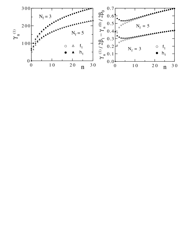
(a)                                                      (b)

Figure 16: Comparison between $f_{1}$ and $h_{1}$ of the variation with $n$ of (a) the two-loop anomalous dimensions $\gamma^{(1)}_{n}$ for $N_{f}=3$ (circles) and 5 (triangles), and (b) the combination $\gamma^{(1)}(n)/2\beta_{1}-\gamma^{(0)}(n)/2\beta_{0}$ for $N_{f}=3$ and 5; from [72].

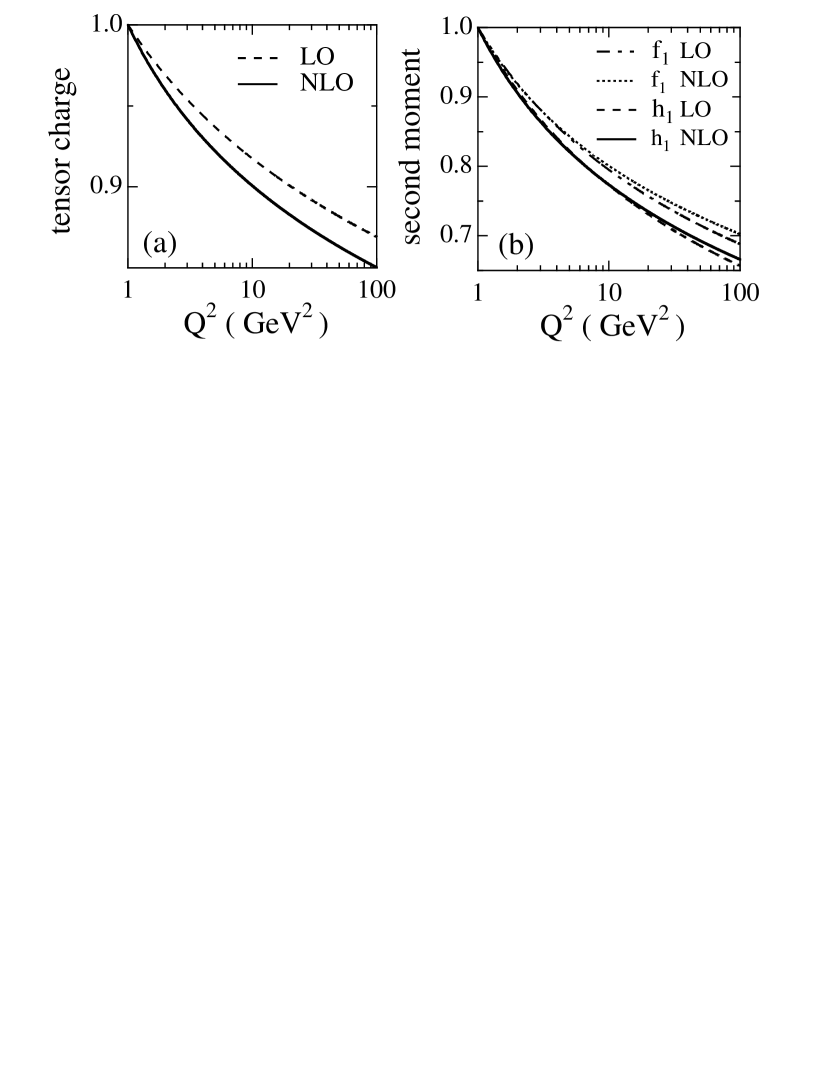
(a)                                                     (b)

Figure 17: The LO and NLO $Q^{2}$-evolution of (a) the tensor charge and (b) the second moments of $h_{1}(x,Q^{2})$ and $f_{1}(x,Q^{2})$ (both are normalised at $Q^{2}=1\,\text{GeV}^{2}$), from [72].

To express the corresponding results in $x$ space it is convenient to introduce the following definitions:

$$\Delta_{T}{R}^{(0)}(x) = \frac{2x}{(1-x)_{+}}\,,$$ (5.3.8)

$$S_{2}(x) = \int_{\frac{x}{1+x}}^{\frac{1}{1+x}}\frac{\d{z}}{z}\ln\left(\frac{1-z}{z}\right)$$ (5.3.9)

$$= -2\text{Li}_{2}(-x)-2\ln{x}\ln(1+x)+{\textstyle\frac{1}{2}}\ln^{2}x-{\textstyle\frac{1}{6}}\pi^{2}\,,$$

where $\text{Li}_{2}(x)$ is the usual dilogarithm function. In the $\overline{\text{MS}}$ scheme, defining

$$\Delta_{T}{P}_{qq,{\pm}}^{(1)}(x)=\Delta_{T}{P}_{qq}^{(1)}(x)\pm\Delta_{T}{P}_{q\mathchoice{\makebox[0.0pt][l]{$\displaystyle\kern 0.90417pt\overline{\kern-1.05487pt\phantom{q}}$}}{\makebox[0.0pt][l]{$\textstyle\kern 0.90417pt\overline{\kern-1.05487pt\phantom{q}}$}}{\makebox[0.0pt][l]{$\scriptstyle\kern 0.63292pt\overline{\kern-0.7384pt\phantom{q}}$}}{\makebox[0.0pt][l]{$\scriptscriptstyle\kern 0.45209pt\overline{\kern-0.52744pt\phantom{q}}$}}q}^{(1)}(x)\,,$$ (5.3.10)

cf. eq. (5.3.4a), one then has

$$\Delta_{T}{P}_{qq}^{(1)}(x) = C_{\text{F}}^{2}\left\{\rule[-7.3194pt]{0.0pt}{20.23602pt}1-x-\left[{\textstyle\frac{3}{2}}+2\ln(1-x)\right]\ln{x}\,\Delta_{T}{R}^{(0)}(x)\right.$$ (5.3.11a)

$$\hskip 50.00008pt+\left.\rule[-7.3194pt]{0.0pt}{20.23602pt}\left[{\textstyle\frac{3}{8}}-{\textstyle\frac{1}{2}}\pi^{2}+6\zeta(3)\right]\delta(1-x)\right\}$$

$$+ {\textstyle\frac{1}{2}}C_{\text{F}}C_{\text{G}}\left\{\rule[-7.3194pt]{0.0pt}{20.23602pt}-(1-x)+\left[{\textstyle\frac{67}{9}}+{\textstyle\frac{11}{3}}\ln{x}+\ln^{2}x-{\textstyle\frac{1}{3}}\pi^{2}\right]\Delta_{T}{R}^{(0)}(x)\right.$$

$$\hskip 50.00008pt+\left.\rule[-7.3194pt]{0.0pt}{20.23602pt}\left[{\textstyle\frac{17}{12}}+{\textstyle\frac{11}{9}}\pi^{2}-6\zeta(3)\right]\delta(1-x)\right\}$$

$$+ {\textstyle\frac{2}{3}}C_{\text{F}}T_{\text{F}}\left\{\rule[-7.3194pt]{0.0pt}{20.23602pt}\left[-\ln{x}-{\textstyle\frac{5}{3}}\right]\Delta_{T}{R}^{(0)}(x)\right.$$

$$\hskip 50.00008pt-\left.\rule[-7.3194pt]{0.0pt}{20.23602pt}\left[{\textstyle\frac{1}{4}}+{\textstyle\frac{1}{3}}\pi^{2}\right]\delta(1-x)\right\},$$

$$\Delta_{T}{P}_{q\mathchoice{\makebox[0.0pt][l]{$\displaystyle\kern 0.90417pt\overline{\kern-1.05487pt\phantom{q}}$}}{\makebox[0.0pt][l]{$\textstyle\kern 0.90417pt\overline{\kern-1.05487pt\phantom{q}}$}}{\makebox[0.0pt][l]{$\scriptstyle\kern 0.63292pt\overline{\kern-0.7384pt\phantom{q}}$}}{\makebox[0.0pt][l]{$\scriptscriptstyle\kern 0.45209pt\overline{\kern-0.52744pt\phantom{q}}$}}q}^{(1)}(x) = C_{\text{F}}\left[C_{\text{F}}-{\textstyle\frac{1}{2}}C_{\text{G}}\right]\left\{\rule[-7.3194pt]{0.0pt}{20.23602pt}-(1-x)+2S_{2}(x)\,\Delta_{T}{R}^{(0)}(-x)\right\},$$ (5.3.11b)

where $\zeta(3)\approx 1.202057$ is the usual Riemann Zeta function. Note that the plus prescription is to be ignored in $\Delta_{T}{R}^{(0)}(-x)$.

To complete this section we also report on the corresponding NLO calculation for linear (transverse) gluon polarisation [94]. As already noted, $\Delta_{T}{g}$ is precluded in the case of spin-half hadrons – it may, however, be present in objects of spin one, such as the deuteron or indeed even the photon[95].

$$\Delta_{T}{P}_{gg}^{(1)}(x) = C_{\text{G}}^{2}\left[\left({\textstyle\frac{67}{18}}+{\textstyle\frac{1}{2}}\ln^{2}x-2\ln{x}\ln(1-x)-{\textstyle\frac{1}{6}}\pi^{2}\right)\Delta_{T}{R}^{(0)}(x)\right.$$ (5.3.12)

$$\hskip 28.45274pt\left.\hbox{}+\frac{1-x^{3}}{6x}+S_{2}(x)\Delta_{T}{R}^{(0)}(-x)+\left({\textstyle\frac{8}{3}}+3\zeta(3)\right)\delta(1-x)\right]$$

$$+ C_{\text{G}}T_{\text{F}}\left[-{\textstyle\frac{10}{9}}\Delta_{T}{R}^{(0)}(x)+\frac{1-x^{3}}{3x}-{\textstyle\frac{4}{3}}\delta(1-x)\right]$$

$$- C_{\text{F}}T_{\text{F}}\left[\frac{2(1-x^{3})}{3x}+\delta(1-x)\right]\,.$$

The corresponding expression in Mellin-moment space for the anomalous dimensions is

$$\Delta_{T}\gamma_{gg}^{(1)}(n) = C_{\text{G}}^{2}\left[{\textstyle\frac{8}{3}}+{\textstyle\frac{1}{2(n-1)(n+2)}}+S_{1}(n)\left(2S_{2}^{{}^{\prime}}({\textstyle\frac{n}{2}})-{\textstyle\frac{67}{9}}\right)+{\textstyle\frac{1}{2}}S_{3}^{{}^{\prime}}({\textstyle\frac{n}{2}})-4\widetilde{S}(n)\right]$$ (5.3.13)

$$+ C_{\text{G}}T_{\text{F}}\left[-{\textstyle\frac{4}{3}}+{\textstyle\frac{20}{9}}S_{1}(n)+{\textstyle\frac{1}{(n-1)(n+2)}}\right]$$

$$- C_{\text{F}}T_{\text{F}}{\textstyle\frac{n(n+1)}{(n-1)(n+2)}}\,.$$

As noted in [94] the result for the part $\sim C_{\text{F}}T_{\text{F}}$ in (5.3.12) was presented in [95] for the region $x<1$ (corresponding to the two-loop splitting function for linearly polarised gluons into photons). However, the two calculations appear to be at variance: the results of [95] imply a small-$x$ behaviour of $\mathop{\mathcal{O}}\nolimits(1/x^{2})$ for the relevant splitting function, which would then be more singular than the unpolarised case.

There are two aspects of the splitting function (5.3.12) that warrant particular comment. Firstly, the small-$x$ behaviour changes significantly on going from LO to NLO. At LO, the splitting function is $\mathop{\mathcal{O}}\nolimits(x)$ for $x\to 0$ whereas at NLO there are $\mathop{\mathcal{O}}\nolimits(1/x)$ terms (as in the unpolarised case): we have

$$\Delta_{T}{P}_{gg}^{(1)}(x)\approx\frac{1}{6x}\left(N_{\text{c}}^{2}+2N_{\text{c}}T_{\text{F}}-4C_{\text{F}}T_{\text{F}}\right)+\mathop{\mathcal{O}}\nolimits(x)\qquad(x\to 0)\,.$$ (5.3.14)

Notice that all logarithmic terms ${\sim}x\ln^{2}x$ cancel in this limiting region.

The second comment regards the so-called supersymmetric limit: namely $C_{\text{F}}=N_{\text{c}}=2T_{\text{F}}$ [65], which was investigated for the unpolarised and longitudinally polarised NLO splitting functions in [96, 82, 84, 83], for the time-like case in [97] and for the case of transversity in [94]. In the supersymmetric limit the LO splitting functions for quark transversity and for linearly polarised gluons are equal[18, 95]:

$$\Delta_{T}{P}_{qq}^{(0)}(x)=N_{\text{c}}\left[\frac{2x}{(1-x)_{+}}+\frac{3}{2}\delta(1-x)\right]=\Delta{P}_{gg}^{(0)}(x)\,.$$ (5.3.15)

Hence, we may consider linear polarisation of the gluon as the supersymmetric partner to transversity (see also [65]). Indeed, as was natural, we have already applied the terminology without distinction to spin-half and spin-one.

In [94] the check was performed that the supersymmetric relation still holds at NLO. To do so it is necessary to transform to a regularisation scheme that respects supersymmetry, namely dimensional reduction. As noted in [94] the transformation is rendered essentially trivial owing to the absence of $\mathop{\mathcal{O}}\nolimits(\epsilon)$ terms in the $d$-dimensional LO splitting functions for transversity or linearly polarised gluons at $x<1$; such terms are always absent in dimensional reduction but may be present in dimensional regularisation. Thus, at NLO the results for the splitting functions for quark transversity – see eqs. (5.3.11a, LABEL:subeq:qcd-DTP1qqbar) – and for linearly polarised gluons, eq. (5.3.12), automatically coincide for $x<1$ with their respective $\overline{\text{MS}}$ expressions in dimensional reduction. These expressions may therefore be immediately compared in the supersymmetric limit and indeed for $C_{\text{F}}=N_{\text{c}}=2T_{\text{F}}$

$$\Delta_{T}{P}_{qq,+}^{(1)}(x)\equiv\Delta_{T}{P}_{gg}^{(1)}(x)\qquad(x<1)\,.$$ (5.3.16)

Note, in addition, that the supersymmetric relation is trivially satisfied for $x=1$; see [84, 83], where the appropriate factorisation-scheme transformation to dimensional reduction for $x=1$ is given.

5.4 Evolution of the transversity distributions

The interest in the effects of evolution in the case of transversity is two-fold: first, there is the obvious question of the relative magnitude of the distributions at high energies given some low-energy starting point (e.g., a non-perturbative model calculation, for a detailed discussion and examples see Sec. 8) and second is the problem raised by the Soffer inequality. It is to the first that we now address our attention while we shall deal with latter shortly.

Let us for the moment simply pose the question of the effect of QCD evolution [98, 99, 100, 101, 102, 72, 103, 104, 105, 106, 107, 108, 74, 109, 110, 111, 112, 94] on the overall magnitude of the transversity densities that might be constructed at some low-energy scale. As already noted above, there is no conservation rule associated with the tensor charge of the nucleon (cf. the vector and axial-vector charges) and, indeed, the sign of the anomalous dimensions at both LO and NLO is such that the first moment of $h_{1}$ falls with increasing $Q^{2}$. Thus, one immediately deduces that the tensor charge will eventually disappear in comparison to the vector and axial charges. Such behaviour could have a dramatic impact on the feasibility of high-energy measurement of $h_{1}$ and thus requires carefully study.

A analytic functional form for the LO anomalous dimensions governing the evolution of $h_{1}$ is

$$\Delta_{T}\gamma^{(0)}(n)={\textstyle\frac{4}{3}}\left\{{\textstyle\frac{3}{2}}-2\left[\psi(n+1)+\gamma_{\text{E}}\right]\right\},$$ (5.4.1)

where $\psi(z)=\frac{\d\ln\Gamma(z)}{\d{z}}$ is the digamma function and $\gamma_{\text{E}}=0.5772157$ is the Euler–Mascheroni constant. Since $\Delta_{T}\gamma^{(0)}(1)=-\frac{2}{3}$, the first moment of $h_{1}$ and the tensor charges, $\delta{q}=\int_{0}^{1}\d{x}\,(\Delta_{T}{q}-\Delta_{T}\mathchoice{\makebox[0.0pt][l]{$\displaystyle\kern 1.29167pt\overline{\kern-1.50696pt\phantom{q}}$}}{\makebox[0.0pt][l]{$\textstyle\kern 1.29167pt\overline{\kern-1.50696pt\phantom{q}}$}}{\makebox[0.0pt][l]{$\scriptstyle\kern 0.90417pt\overline{\kern-1.05487pt\phantom{q}}$}}{\makebox[0.0pt][l]{$\scriptscriptstyle\kern 0.64583pt\overline{\kern-0.75348pt\phantom{q}}$}}q)$, decrease with $Q^{2}$ as

$$\delta{q}(Q^{2}) = \left[\frac{\alpha_{s}(Q^{2})}{\alpha_{s}(Q_{0}^{2})}\right]^{-2\Delta_{T}\gamma_{qq}^{(0)}\!(1)/\beta_{0}{}}\,\delta{q}(Q_{0}^{2})$$ (5.4.2)

$$= \left[\frac{\alpha_{s}(Q_{0}^{2})}{\alpha_{s}(Q^{2})}\right]^{-4/27}\,\delta{q}(Q_{0}^{2})\,,$$

where, to obtain the second equality, we have set $N_{\text{f}}=3$. Despite the smallness of the exponent, $-4/27$, we shall see that the evolution of $\Delta_{T}{q}(x,Q^{2})$ is rather different from that of the helicity distributions $\Delta{q}(x,Q^{2})$, especially for small $x$. At NLO this becomes

$$\delta{q}(Q^{2}) = \left[\frac{\alpha_{s}(Q^{2})}{\alpha_{s}(Q_{0}^{2})}\right]^{-2\Delta_{T}\gamma_{qq}^{(0)}\!(1)/\beta_{0}}$$ (5.4.3)

$$\hbox{}\times\left[1+\frac{\alpha_{s}(Q_{0}^{2})-\alpha_{s}(Q^{2})}{\pi\beta_{0}}\left(\Delta_{T}\gamma_{qq,-}^{(1)}(1)-\frac{\beta_{1}}{2\beta_{0}}\,\Delta_{T}\gamma_{qq}^{(0)}(1)\right)\right]\delta{q}(Q_{0}^{2})$$

$$= \left[\frac{\alpha_{s}(Q^{2})}{\alpha_{s}(Q_{0}^{2})}\right]^{\frac{4}{27}}\left[\rule[-9.04166pt]{0.0pt}{23.68048pt}1-\frac{337}{486\pi}\left(\alpha_{s}(Q_{0}^{2})-\alpha_{s}(Q^{2})\right)\right],$$

where in the second equality we have used

$$\Delta_{T}\gamma_{qq,-}^{(1)}(1)=\frac{19}{8}\,C_{\text{F}}^{2}-\frac{257}{72}\,C_{\text{F}}N_{\text{c}}+\frac{13}{18}\,C_{\text{F}}T_{\text{F}}=-\frac{181}{18}+\frac{13}{27}\,N_{\text{f}}\,,$$ (5.4.4)

and we have once again set $N_{\text{f}}=3$.

Recall that the first moments of the $q\to{qg}$ polarised and unpolarised splitting functions, vanish to all orders in perturbation theory and that the $g\to{q}\mathchoice{\makebox[0.0pt][l]{$\displaystyle\kern 1.29167pt\overline{\kern-1.50696pt\phantom{q}}$}}{\makebox[0.0pt][l]{$\textstyle\kern 1.29167pt\overline{\kern-1.50696pt\phantom{q}}$}}{\makebox[0.0pt][l]{$\scriptstyle\kern 0.90417pt\overline{\kern-1.05487pt\phantom{q}}$}}{\makebox[0.0pt][l]{$\scriptscriptstyle\kern 0.64583pt\overline{\kern-0.75348pt\phantom{q}}$}}q$ polarised anomalous dimension $\Delta\gamma_{qg}(1)$ is zero at LO; thus, $\Delta{q}(Q^{2})$ is constant. This can be seen analytically by the following argument [99] based on the double-log approximation. The leading behaviour of the parton distributions for small $x$ is governed by the rightmost singularity of their anomalous dimensions in Mellin-moment space. From eq. (5.4.1) we see that this singularity is located at $n=-1$ for $\Delta_{T}{q}$ at LO. Expanding $\Delta_{T}\gamma(n)$ around this point gives

$$\Delta_{T}\gamma(n)\sim\frac{8}{3(n+1)}+\mathop{\mathcal{O}}\nolimits(1)\,.$$ (5.4.5)

Equivalently, in $x$-space, expanding the splitting function $\Delta_{T}{P}$ in powers of $x$ yields

$$\Delta_{T}{P}(x)\sim\frac{8}{3}x+\mathop{\mathcal{O}}\nolimits(x^{2})\,.$$ (5.4.6)

In contrast, the rightmost singularity for $\Delta{q}$ in moment space is located at $n=0$ and the splitting functions $\Delta{P}_{qq}$ and $\Delta{P}_{qg}$ behave as constants as $x\to 0$. Therefore, owing to QCD evolution, $\Delta_{T}{q}$ acquires and an extra suppression factor of one power of $x$ with respect to $\Delta{q}$ at small $x$. We note too that at NLO the rightmost singularity for $\Delta_{T}{q}$ is located at $n=0$, so that NLO evolution renders the DGLAP asymptotics for $x\to 0$ in the case of transversity compatible with Regge theory[113].

As mentioned earlier, this problem may be investigated numerically by integrating the DGLAP equations (5.1.11) with suitable starting input for $h_{1}$ and $g_{1}$. As a reasonable trial model one may assume the various $\Delta_{T}{q}$ and $\Delta{q}$ to be equal at some small scale $Q_{0}^{2}$ and then allow the two types of distributions to evolve separately, each according to its own evolution equations. The input hypothesis $\Delta_{T}{q}(x,Q_{0}^{2})=\Delta{q}(x,Q_{0}^{2})$ is suggested by various quark-model calculations of $\Delta_{T}{q}$ and $\Delta{q}$ [14, 98] (see also Sec. 8 here), in which these two distributions are found to be very similar at a scale $Q_{0}^{2}\lesssim 0.5\,\text{GeV}^{2}$. For $\Delta{q}(x,Q_{0}^{2})$, we then use the leading-order Glück-Reya-Vogelsang (GRV) parametrisation [114], whose input scale is $Q_{0}^{2}=0.23\,\text{GeV}^{2}$. The result for the $u$-quark distributions is shown in Fig. 18 (the situation is similar for the other flavours). The dashed line is the input, the solid line and the dotted line are the results of the evolution of $\Delta_{T}{u}$ and $\Delta{u}$, respectively, at $Q^{2}=25\,\text{GeV}^{2}$. For completeness, the evolution of $\Delta_{T}{u}$ when driven only by $P_{qq}$ – i.e., with the $\Delta_{T}{P}$ term turned off, see eq. (5.2.3c) – is also shown (dot–dashed line). The large difference in the evolution of $\Delta_{T}{u}$ (solid curve) and $\Delta{u}$ (dotted curve) at small $x$ is evident. Note also the difference between the correct evolution of $\Delta_{T}{u}$ and the evolution driven purely by $P_{qq}$ (dot–dashed curve).

Figure 18: Evolution of the helicity and transversity distributions for the $u$ flavour [99]. The dashed curve is the input $\Delta_{T}{u}=\Delta{u}$ at $Q_{0}^{2}=0.23\,\text{GeV}^{2}$ taken from the GRV [114] parametrisation. The solid (dotted) curve is $\Delta_{T}{u}$ ($\Delta{u}$) at $Q^{2}=25\,\text{GeV}^{2}$. The dot–dashed curve is the result of the evolution of $\Delta_{T}{u}$ at $Q^{2}=25\,\text{GeV}^{2}$ driven by $P_{qq}$, i.e., with the term $\Delta_{T}{P}$ in $P_{h}$ turned off.

As a further comparison of the behaviour of $h_{1}$ and $g_{1}$, in Figs. 19 (a) and (b) we display the LO and NLO $Q^{2}$-evolution of $\Delta_{T}{u}$ and $\Delta{u}$, starting respectively from the LO and NLO input function for $\Delta{u}$ given in [88] for $Q^{2}=0.23$ and $0.34\,\text{GeV}^{2}$. Although LO evolution leads to a significant divergence between $\Delta_{T}{u}$ and $\Delta{u}$ at $Q^{2}=20\,\text{GeV}^{2}$, this tendency is strengthened by the NLO evolution, in particular, in the small-$x$ region. Although the evolution of $\Delta{u}$ shown in Fig. 19 is affected by mixing with the gluon distribution, the non-singlet quark distributions also show the same trend.

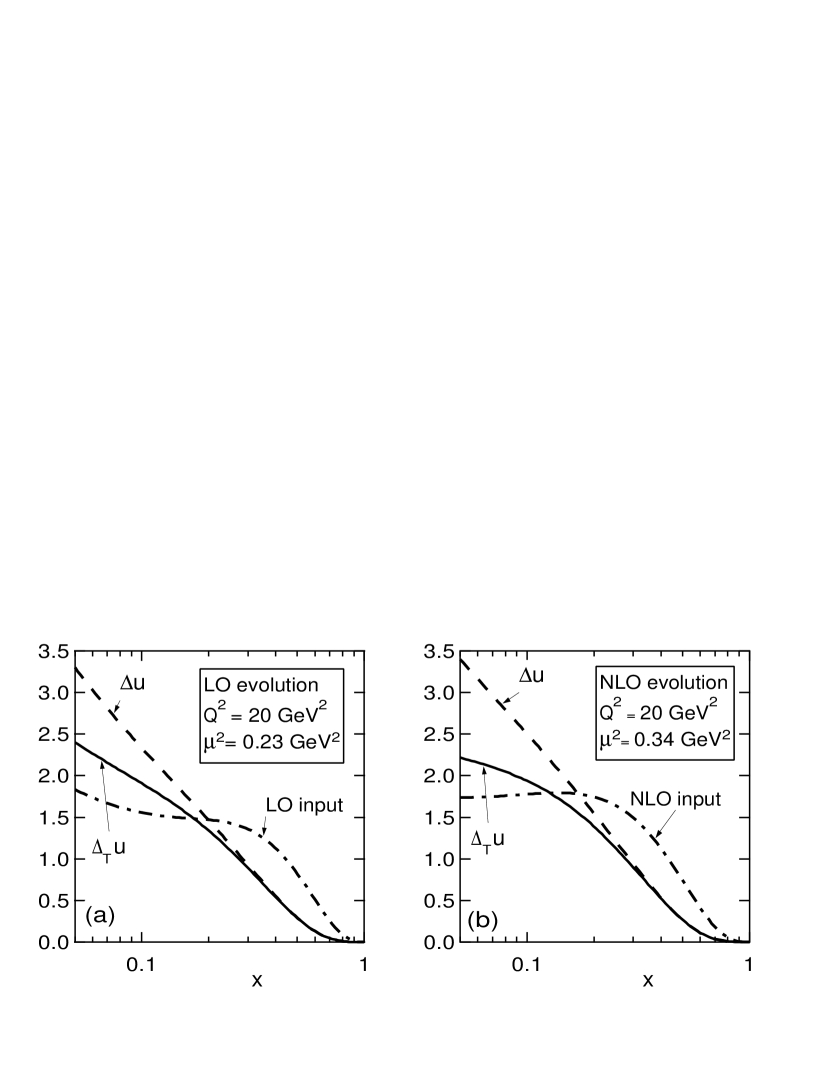
(a)                                                           (b)

Figure 19: Comparison of the $Q^{2}$-evolution of $\Delta_{T}{u}(x,Q^{2})$ and $\Delta{u}(x,Q^{2})$ at (a) LO and (b) NLO, from [72].

In Fig. 20, we compare the NLO $Q^{2}$-evolution of $\Delta_{T}\mathchoice{\makebox[0.0pt][l]{$\displaystyle\kern 1.29167pt\overline{\kern-1.50696pt\phantom{u}}$}}{\makebox[0.0pt][l]{$\textstyle\kern 1.29167pt\overline{\kern-1.50696pt\phantom{u}}$}}{\makebox[0.0pt][l]{$\scriptstyle\kern 0.90417pt\overline{\kern-1.05487pt\phantom{u}}$}}{\makebox[0.0pt][l]{$\scriptscriptstyle\kern 0.64583pt\overline{\kern-0.75348pt\phantom{u}}$}}u$, $\Delta_{T}\mathchoice{\makebox[0.0pt][l]{$\displaystyle\kern 2.08334pt\overline{\kern-2.43059pt\phantom{d}}$}}{\makebox[0.0pt][l]{$\textstyle\kern 2.08334pt\overline{\kern-2.43059pt\phantom{d}}$}}{\makebox[0.0pt][l]{$\scriptstyle\kern 1.45834pt\overline{\kern-1.7014pt\phantom{d}}$}}{\makebox[0.0pt][l]{$\scriptscriptstyle\kern 1.04167pt\overline{\kern-1.21529pt\phantom{d}}$}}d$ and $\Delta\mathchoice{\makebox[0.0pt][l]{$\displaystyle\kern 1.29167pt\overline{\kern-1.50696pt\phantom{u}}$}}{\makebox[0.0pt][l]{$\textstyle\kern 1.29167pt\overline{\kern-1.50696pt\phantom{u}}$}}{\makebox[0.0pt][l]{$\scriptstyle\kern 0.90417pt\overline{\kern-1.05487pt\phantom{u}}$}}{\makebox[0.0pt][l]{$\scriptscriptstyle\kern 0.64583pt\overline{\kern-0.75348pt\phantom{u}}$}}u$, starting from the same input distribution function (the NLO input function for the sea-quark distribution to $g_{1}$ given in [88]). The difference between $\Delta_{T}\mathchoice{\makebox[0.0pt][l]{$\displaystyle\kern 1.29167pt\overline{\kern-1.50696pt\phantom{u}}$}}{\makebox[0.0pt][l]{$\textstyle\kern 1.29167pt\overline{\kern-1.50696pt\phantom{u}}$}}{\makebox[0.0pt][l]{$\scriptstyle\kern 0.90417pt\overline{\kern-1.05487pt\phantom{u}}$}}{\makebox[0.0pt][l]{$\scriptscriptstyle\kern 0.64583pt\overline{\kern-0.75348pt\phantom{u}}$}}u$ and $\Delta\mathchoice{\makebox[0.0pt][l]{$\displaystyle\kern 1.29167pt\overline{\kern-1.50696pt\phantom{u}}$}}{\makebox[0.0pt][l]{$\textstyle\kern 1.29167pt\overline{\kern-1.50696pt\phantom{u}}$}}{\makebox[0.0pt][l]{$\scriptstyle\kern 0.90417pt\overline{\kern-1.05487pt\phantom{u}}$}}{\makebox[0.0pt][l]{$\scriptscriptstyle\kern 0.64583pt\overline{\kern-0.75348pt\phantom{u}}$}}u$ is again significant. Although the input sea-quark distribution is taken to be flavour symmetric ($\Delta_{T}\mathchoice{\makebox[0.0pt][l]{$\displaystyle\kern 1.29167pt\overline{\kern-1.50696pt\phantom{u}}$}}{\makebox[0.0pt][l]{$\textstyle\kern 1.29167pt\overline{\kern-1.50696pt\phantom{u}}$}}{\makebox[0.0pt][l]{$\scriptstyle\kern 0.90417pt\overline{\kern-1.05487pt\phantom{u}}$}}{\makebox[0.0pt][l]{$\scriptscriptstyle\kern 0.64583pt\overline{\kern-0.75348pt\phantom{u}}$}}u=\Delta_{T}\mathchoice{\makebox[0.0pt][l]{$\displaystyle\kern 2.08334pt\overline{\kern-2.43059pt\phantom{d}}$}}{\makebox[0.0pt][l]{$\textstyle\kern 2.08334pt\overline{\kern-2.43059pt\phantom{d}}$}}{\makebox[0.0pt][l]{$\scriptstyle\kern 1.45834pt\overline{\kern-1.7014pt\phantom{d}}$}}{\makebox[0.0pt][l]{$\scriptscriptstyle\kern 1.04167pt\overline{\kern-1.21529pt\phantom{d}}$}}d$ at $Q^{2}=0.34\,\text{GeV}^{2}$), NLO evolution violates this symmetry owing to the appearance of $\Delta_{T}{P}_{q\mathchoice{\makebox[0.0pt][l]{$\displaystyle\kern 0.90417pt\overline{\kern-1.05487pt\phantom{q}}$}}{\makebox[0.0pt][l]{$\textstyle\kern 0.90417pt\overline{\kern-1.05487pt\phantom{q}}$}}{\makebox[0.0pt][l]{$\scriptstyle\kern 0.63292pt\overline{\kern-0.7384pt\phantom{q}}$}}{\makebox[0.0pt][l]{$\scriptscriptstyle\kern 0.45209pt\overline{\kern-0.52744pt\phantom{q}}$}}q}^{(1)}$ – see (5.3.11b). However, this effect is very small, as is evident from Fig. 20 and discussed in [105].

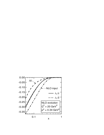
Figure 20: Comparison of the NLO $Q^{2}$-evolution of $\Delta_{T}\bar{u}(x,Q^{2})$, $\Delta_{T}\bar{d}(x,Q^{2})$ and $\Delta\bar{u}(x,Q^{2})$, from [72].

5.5 Evolution of the Soffer inequality and general positivity constraints

Particular interest in the effects of evolution arises in connection with the Soffer inequality [38], eq. (4.6.6). It has been argued [115] that this inequality, which was derived within a parton model framework, may be spoilt by radiative corrections, much as the Callan–Gross relation. Such an analogy, however, is somewhat misleading, since the Soffer inequality is actually very similar to the more familiar positivity bound $|\Delta{q}(x)|\leq{q}(x)$. The LO evolution of the inequality is governed by eq. (5.2.4) and hence it is not endangered, as pointed out in [99]. At NLO the situation is complicated by the well-known problems of scheme dependence etc.

Indeed, it is perhaps worth remarking that the entire question of positivity is ill-defined beyond LO, inasmuch as the parton distributions themselves as physical quantities become ill-defined: a priori there is no guarantee in a given scheme that any form of positivity will survive higher-order corrections. This observation may, of course, be turned on its head and used to impose conditions on the scheme choice such that positivity will be guaranteed [116]. At any rate, if this is possible then at the hadronic level any natural positivity bounds should be respected, independently of the regularisation scheme applied.

An instructive and rather general manner to examine the problem is to recast the system of evolution equations into a form analogous to the Boltzmann equation [101]. First of all, let us rewrite eq. (5.1.11) in a slightly more suggestive form for the non-singlet case:

$$\frac{\d{q}(x,t)}{\d{t}}=\int_{x}^{1}\frac{\d{y}}{y}\;P\!\left(\frac{x}{y},t\right)q(y,t)\,,$$ (5.5.1)

where $t=\ln{Q^{2}}$. One may thus interpret the equation as describing the time, $t$, evolution of densities, $f(x,t)$, in a one-dimensional $x$ space. The flow is constrained to run from large to small $x$ owing to the ordering $x<y$ under the integral. Such an interpretation facilitates dealing with the infrared (IR) singularities present in the expressions for $P(x)$. Indeed, a key element is provided by consideration of precisely the IR singularities[117, 118].

Let us now rewrite the plus regularisation in the following form:

$$P_{+}(x,t)=P(x,t)-\delta(1-x)\int_{0}^{1}\frac{\d{y}}{y}\;P(y,t)\,,$$ (5.5.2)

which then permits the evolution equations to be rewritten as

$$\frac{\d{q}(x,t)}{\d{t}}=\int_{x}^{1}\frac{\d{y}}{y}\;q(y,t)\,P\!\left(\frac{x}{y},t\right)-q(x,t)\int_{0}^{1}\d{y}\;P(y,t)\,.$$ (5.5.3)

Reading the second term as describing the flow of partons at the point $x$ [117], the kinetic interpretation is immediate. It is useful to render the analogy more direct by the change of variables $y\to{y/x}$ in the second term, leading to the following more symmetric form:

$$\frac{\d{q}(x,t)}{\d{t}}=\int_{x}^{1}\frac{\d{y}}{y}\;q(y,t)\,P\!\left(\frac{x}{y},t\right)-\int_{0}^{x}\frac{\d{y}}{x}\;q(x,t)\,P\!\left(\frac{y}{x},t\right).$$ (5.5.4)

In this fashion the equation has been translated into a form analogous to the Boltzmann equation: namely,

$$\frac{\d{q}(x,t)}{\d{t}}=\int_{0}^{1}\d{y}\left[\sigma(y\to x;t)\,q(y,t)-\sigma(x\to y;t)\,q(x,t)\right],$$ (5.5.5)

where the one-dimensional analogue of the Boltzmann “scattering probability” may be defined as

$$\sigma(y\to x;t)=\theta(y-x)\,\frac{1}{y}\,P\!\left(\frac{x}{y},t\right).$$ (5.5.6)

Cancellation of the IR divergencies between contributions involving real and virtual gluons is therefore seen to occur as a consequence of the continuity condition on “particle number”; i.e., the equality of flow in and out in the neighbourhood of $y=x$ in both terms of eq. (5.5.5).

In the spin-averaged case the particle density (at some initialisation point) is positive by definition. Now, the negative second term in eq. (5.5.5) cannot change the sign of the distribution because it is “diagonal” in $x$, i.e., it is proportional to the function at the same point $x$. When the distribution is sufficiently close to zero, it stops decreasing. This is true for both “plus” and $\delta(1-x)$ terms, for any value of their coefficients (if positive, it only reinforces positivity of the distribution).

Turning next to the spin-dependent case, for simplicity we consider first the flavour non-singlet and allow the spin-dependent and spin-independent kernels to be different, as they indeed are at NLO. Rather than the usual helicity sums and differences, it turns out to be convenient to cast the equations in terms of definite parton helicities. Although such a form mixes contributions of different helicities, the positivity properties emerge more clearly. We thus have

$$\frac{\d{q}_{+}(x,t)}{\d{t}}=P_{++}(x,t)\otimes q_{+}(x,t)+P_{+-}(x,t)\otimes q_{-}(x,t)\,,$$ (5.5.7a)

$$\frac{\d{q}_{-}(x,t)}{\d{t}}=P_{+-}(x,t)\otimes q_{+}(x,t)+P_{++}(x,t)\otimes q_{-}(x,t)\,,$$ (5.5.7b)

where $P_{+\mathbin{\mathchoice{\raisebox{-0.57263pt}{$\displaystyle\pm$}}{\raisebox{-0.57263pt}{$\textstyle\pm$}}{\raisebox{-0.43399pt}{$\scriptstyle\pm$}}{\raisebox{-0.3014pt}{$\scriptscriptstyle\pm$}}}}(z,t)={\textstyle\frac{1}{2}}[P(z,t)\pm\Delta{P}(z,t)]$ are the evolution kernels for helicity non-flip and flip respectively. For $x<y$, positivity of the initial distributions, $q_{\pm}(x,t_{0})\geq 0$ or $|\Delta{q}(x,t_{0})|\leq{q}(x,t_{0})$, is preserved if both kernels $P_{+\mathbin{\mathchoice{\raisebox{-0.57263pt}{$\displaystyle\pm$}}{\raisebox{-0.57263pt}{$\textstyle\pm$}}{\raisebox{-0.43399pt}{$\scriptstyle\pm$}}{\raisebox{-0.3014pt}{$\scriptscriptstyle\pm$}}}}$ are positive, which is true if

$$|\Delta{P}(z,t)|\leq P(z,t)\qquad(z<1)\,.$$ (5.5.8)

Terms that are singular at $z=1$ cannot alter positivity as they only appear in the diagonal (in helicity) kernel, $P_{++}$; non-forward scattering is completely IR safe. Once again in the kinetic interpretation, the distributions $q_{+}$ and $q_{-}$ stop decreasing on approaching zero.

To extend the proof to include the case in which there is quark–gluon mixing is trivial—we need the full expressions for the evolutions of quark and gluon distributions of each helicity:

$$\frac{\d{q}_{+}(x,t)}{{\d{t}}} = P_{++}^{qq}(x,t)\otimes q_{+}(x,t)+P_{+-}^{qq}(x,t)\otimes q_{-}(x,t)$$ (5.5.9a)

$$+ P_{++}^{qg}(x,t)\otimes g_{+}(x,t)+P_{+-}^{qg}(x,t)\otimes g_{-}(x,t)\,,$$

$$\frac{\d{q}_{-}(x,t)}{{\d{t}}} = P_{+-}^{qg}(x,t)\otimes q_{+}(x,t)+P_{++}^{qg}(x,t)\otimes q_{-}(x,t)$$ (5.5.9b)

$$+ P_{+-}^{qg}(x,t)\otimes g_{+}(x,t)+P_{++}^{qg}(x,t)\otimes g_{-}(x,t)\,,$$

$$\frac{\d{g}_{+}(x,t)}{{\d{t}}} = P_{++}^{gq}(x,t)\otimes q_{+}(x,t)+P_{+-}^{gq}(x,t)\otimes q_{-}(x,t)$$ (5.5.9c)

$$+ P_{++}^{gg}(x,t)\otimes g_{+}(x,t)+P_{+-}^{gg}(x,t)\otimes g_{-}(x,t)\,,$$

$$\frac{\d{g}_{-}(x,t)}{{\d{t}}} = P_{+-}^{gq}(x,t)\otimes q_{+}(x,t)+P_{++}^{gq}(x,t)\otimes q_{-}(x,t)$$ (5.5.9d)

$$+ P_{+-}^{gg}(x,t)\otimes g_{+}(x,t)+P_{++}^{gg}(x,t)\otimes g_{-}(x,t)\,.$$

Since inequality (5.5.8) is clearly valid separately for each type of parton[116],

$$|\Delta{P}_{ij}(z,t)|\leq P_{ij}(z,t)\qquad(z<1,\quad i,j=q,g)\,,$$ (5.5.10)

all the kernels appearing on the r.h.s. of this system, are positive. With regard to the singular terms, they are again diagonal (in parton type here) and hence cannot affect positivity. The validity of the equations at LO is guaranteed via their derivation, just as the (positive) helicity-dependent kernels were in fact first calculated in [12]. At NLO, the situation is more complex[116].

To conclude, the maintenance of positivity under $Q^{2}$ evolution has two sources: (a) inequalities (5.5.10), leading to the increase of distributions and (b) the kinetic interpretation of the decreasing terms. For the latter, it is crucial that they are diagonal in $x$, helicity and also parton type, which is a prerequisite for their IR nature.

We now finally return to the Soffer inequality: in analogy with the previous analysis, it is convenient to define the following “super” distributions

$$Q_{+}(x) = q_{+}(x)+\Delta_{T}{q}(x)\,,$$ (5.5.11a)

$$Q_{-}(x) = q_{+}(x)-\Delta_{T}{q}(x)\,.$$ (5.5.11b)

According to the Soffer inequality, both distributions are positive at some scale (say $Q^{2}_{0}$) and the evolution equations for the non-singlet case take the form (henceforth the argument $t$ will be suppressed)

$$\frac{\d{Q}_{+}(x)}{\d{t}} = P^{Q}_{++}(x)\otimes Q_{+}(x)+P^{Q}_{+-}(x)\otimes Q_{-}(x)\,,$$ (5.5.12a)

$$\frac{\d{Q}_{-}(x)}{\d{t}} = P^{Q}_{+-}(x)\otimes Q_{+}(x)+P^{Q}_{++}(x)\otimes Q_{-}(x))\,,$$ (5.5.12b)

where the “super” kernels at LO are just

$$P^{Q}_{++}(z) = {\textstyle\frac{1}{2}}[P_{qq}^{(0)}(z)+P_{h}^{(0)}(z)]$$ (5.5.13a)

$$= {\textstyle\frac{1}{2}}C_{\text{F}}\left[\frac{(1+z)^{2}}{(1-z)_{+}}+3\delta(1-z)\right],$$

$$P^{Q}_{+-}(z) = {\textstyle\frac{1}{2}}[P_{qq}^{(0)}(z)-P_{h}^{(0)}(z)]$$ (5.5.13b)

$$= {\textstyle\frac{1}{2}}C_{\text{F}}(1-z)\,.$$

One can easily see, that the inequalities analogous to (5.5.10) are satisfied, so that both $P^{Q}_{++}(z)$ and $P^{Q}_{+-}(z)$ are positive for $z<1$, while the singular term appears only in the diagonal kernel. Thus, both requirements are fulfilled and the Soffer inequality is maintained under LO evolution. The extension to the singlet case is trivial owing to the exclusion of gluon mixing. Therefore, only evolution of quarks is affected, leading to the presence of the same extra terms on the r.h.s., as in eqs. (5.5.9a):

$$\frac{\d{Q}_{+}(x)}{\d{t}} = P_{++}^{Q}(x)\otimes Q_{+}(x)+P_{+-}^{Q}(x)\otimes Q_{-}(x)$$ (5.5.14a)

$$+ P_{+-}^{qG}(x)\otimes G_{+}(x)+P_{++}^{qG}(x)\otimes G_{-}(x)\,,$$

$$\frac{\d{Q}_{-}(x)}{\d{t}} = P_{+-}^{Q}(x)\otimes Q_{+}(x)+P_{++}^{Q}(x)\otimes Q_{-}(x)$$ (5.5.14b)

$$+ P_{+-}^{qG}(x)\otimes G_{+}(x)+P_{++}^{qG}(x)\otimes G_{-}(x)\,,$$

which are all positive and singularity free; this concludes the demonstration that positivity is indeed preserved.

6 Transversity in semi-inclusive leptoproduction

While it is usual to adopt DIS as the defining process and point of reference when discussing distribution functions, as repeatedly noted and explicitly shown in Sec. 3, the case of transversity is somewhat special in that it does not appear in DIS. However, owing to the topology of the contributing Feynman diagrams, transversity does play a rôle in semi-inclusive DIS, owing to the presence of two hadrons: one in the initial state and the other in the final state [18, 119, 20, 17, 120, 121, 122]. This process is the subject of the present section.

6.1 Definitions and kinematics

Semi-inclusive – or, to be more precise, single-particle inclusive – leptoproduction (see Fig. 21) is a DIS reaction in which a hadron $h$, produced in the current fragmentation region, is detected in the final state (for the general formalism see [123, 15])

$$l(\ell)\,+\,N(P)\to l^{\prime}(\ell^{\prime})\,+\,h(P_{h})\,+\,X(P_{X})\,.$$ (6.1.1)

With a transversely polarised target, one can measure quark transverse polarisation at leading twist either by looking at a possible asymmetry in the $\mathchoice{\mbox{\boldmath$\displaystyle P$\unboldmath}}{\mbox{\boldmath$\textstyle P$\unboldmath}}{\mbox{\boldmath$\scriptstyle P$\unboldmath}}{\mbox{\boldmath$\scriptscriptstyle P$\unboldmath}}_{h\perp}$ distribution of the produced hadron (the so-called Collins effect [17, 124, 16, 15]), or by polarimetry of a transversely polarised final hadron (for instance, a $\Lambda^{0}$ hyperon) [18, 125, 126, 15]. Transversity distributions also appear in the $\mathchoice{\mbox{\boldmath$\displaystyle P$\unboldmath}}{\mbox{\boldmath$\textstyle P$\unboldmath}}{\mbox{\boldmath$\scriptstyle P$\unboldmath}}{\mbox{\boldmath$\scriptscriptstyle P$\unboldmath}}_{h\perp}$-integrated cross-section at higher twist [120, 15].

Figure 21: Semi-inclusive deeply-inelastic scattering.

We define the invariants

$$x=\frac{Q^{2}}{2P{\cdot}q}\,,\quad y=\frac{P{\cdot}q}{P{\cdot}\ell}\,,\quad z=\frac{P{\cdot}P_{h}}{P{\cdot}q}\,.$$ (6.1.2)

We shall be interested in the limit where $Q^{2}\equiv-q^{2},P{\cdot}q,P_{h}{\cdot}q$ and $P_{h}{\cdot}P$ become large while $x$ and $z$ remain finite.

The geometry of the process is shown in Fig. 22. The lepton scattering plane is identified by $\textstyle\ell$ and $\mathchoice{\mbox{\boldmath$\displaystyle\ell$\unboldmath}}{\mbox{\boldmath$\textstyle\ell$\unboldmath}}{\mbox{\boldmath$\scriptstyle\ell$\unboldmath}}{\mbox{\boldmath$\scriptscriptstyle\ell$\unboldmath}}^{\prime}$. The virtual photon is taken to move along the $z$-axis. The three-momenta of the virtual photon $\textstyle q$ and of the produced hadron $\mathchoice{\mbox{\boldmath$\displaystyle P$\unboldmath}}{\mbox{\boldmath$\textstyle P$\unboldmath}}{\mbox{\boldmath$\scriptstyle P$\unboldmath}}{\mbox{\boldmath$\scriptscriptstyle P$\unboldmath}}_{h}$ define a second plane, which we call the hadron plane. The spin $S$ of the nucleon and the spin $S_{h}$ of the produced hadron satisfy $S^{2}=S_{h}^{2}=-1$ and $S{\cdot}P=S_{h}{\cdot}P_{h}=0$.

The cross-section for the reaction (6.1.1) is

$$\d\sigma = \frac{1}{4\ell{\cdot}P}\,\sum_{s_{l^{\prime}}}\sum_{X}\int\!\frac{{\d^{3}}\mathchoice{\mbox{\boldmath$\displaystyle P$\unboldmath}}{\mbox{\boldmath$\textstyle P$\unboldmath}}{\mbox{\boldmath$\scriptstyle P$\unboldmath}}{\mbox{\boldmath$\scriptscriptstyle P$\unboldmath}}_{X}}{(2\pi)^{3}\,2E_{X}}$$ (6.1.3)

$$\hbox{}\times(2\pi)^{4}\,\delta^{4}(P+\ell-P_{X}-P_{h}-\ell^{\prime})\,|\mathcal{M}|^{2}\,\frac{{\d}^{3}\mathchoice{\mbox{\boldmath$\displaystyle\ell$\unboldmath}}{\mbox{\boldmath$\textstyle\ell$\unboldmath}}{\mbox{\boldmath$\scriptstyle\ell$\unboldmath}}{\mbox{\boldmath$\scriptscriptstyle\ell$\unboldmath}}^{\prime}}{(2\pi)^{3}\,2E^{\prime}}\,\frac{\d^{3}\mathchoice{\mbox{\boldmath$\displaystyle P$\unboldmath}}{\mbox{\boldmath$\textstyle P$\unboldmath}}{\mbox{\boldmath$\scriptstyle P$\unboldmath}}{\mbox{\boldmath$\scriptscriptstyle P$\unboldmath}}_{h}}{(2\pi)^{3}\,2E_{h}}\,,\qquad$$

where we have summed over the spin $s_{l^{\prime}}$ of the outgoing lepton. The squared matrix element in (6.1.3) is

$$|\mathcal{M}|^{2} = \frac{e^{4}}{q^{4}}\left[\mathchoice{\makebox[0.0pt][l]{$\displaystyle\kern 1.29167pt\overline{\kern-1.50696pt\phantom{u}}$}}{\makebox[0.0pt][l]{$\textstyle\kern 1.29167pt\overline{\kern-1.50696pt\phantom{u}}$}}{\makebox[0.0pt][l]{$\scriptstyle\kern 0.90417pt\overline{\kern-1.05487pt\phantom{u}}$}}{\makebox[0.0pt][l]{$\scriptscriptstyle\kern 0.64583pt\overline{\kern-0.75348pt\phantom{u}}$}}u_{l^{\prime}}(\ell^{\prime},s_{l^{\prime}})\gamma_{\mu}u_{l}(\ell,s_{l})\right]^{*}\left[\mathchoice{\makebox[0.0pt][l]{$\displaystyle\kern 1.29167pt\overline{\kern-1.50696pt\phantom{u}}$}}{\makebox[0.0pt][l]{$\textstyle\kern 1.29167pt\overline{\kern-1.50696pt\phantom{u}}$}}{\makebox[0.0pt][l]{$\scriptstyle\kern 0.90417pt\overline{\kern-1.05487pt\phantom{u}}$}}{\makebox[0.0pt][l]{$\scriptscriptstyle\kern 0.64583pt\overline{\kern-0.75348pt\phantom{u}}$}}u_{l^{\prime}}(\ell^{\prime},s_{l^{\prime}})\gamma_{\nu}u_{l}(\ell,s_{l})\right]$$ (6.1.4)

$$\hbox{}\times\langle X,P_{h}S_{h}|J^{\mu}(0)|PS\rangle^{*}\langle X,P_{h}S_{h}|J^{\nu}(0)|PS\rangle\,,$$

Introducing the leptonic tensor

$$L_{\mu\nu} = \sum_{s_{l^{\prime}}}\left[\mathchoice{\makebox[0.0pt][l]{$\displaystyle\kern 1.29167pt\overline{\kern-1.50696pt\phantom{u}}$}}{\makebox[0.0pt][l]{$\textstyle\kern 1.29167pt\overline{\kern-1.50696pt\phantom{u}}$}}{\makebox[0.0pt][l]{$\scriptstyle\kern 0.90417pt\overline{\kern-1.05487pt\phantom{u}}$}}{\makebox[0.0pt][l]{$\scriptscriptstyle\kern 0.64583pt\overline{\kern-0.75348pt\phantom{u}}$}}u_{l^{\prime}}(\ell^{\prime},s_{l^{\prime}})\gamma_{\mu}u_{l}(\ell,s_{l})\right]^{*}\left[\mathchoice{\makebox[0.0pt][l]{$\displaystyle\kern 1.29167pt\overline{\kern-1.50696pt\phantom{u}}$}}{\makebox[0.0pt][l]{$\textstyle\kern 1.29167pt\overline{\kern-1.50696pt\phantom{u}}$}}{\makebox[0.0pt][l]{$\scriptstyle\kern 0.90417pt\overline{\kern-1.05487pt\phantom{u}}$}}{\makebox[0.0pt][l]{$\scriptscriptstyle\kern 0.64583pt\overline{\kern-0.75348pt\phantom{u}}$}}u_{l^{\prime}}(\ell^{\prime},s_{l^{\prime}})\gamma_{\nu}u_{l}(\ell,s_{l})\right]$$ (6.1.5)

$$= 2(\ell_{\mu}\ell^{\prime}_{\nu}+\ell_{\nu}\ell^{\prime}_{\mu}-g_{\mu\nu}\,\ell{\cdot}\ell^{\prime})+2\text{i}\,\lambda_{l}\,\varepsilon_{\mu\nu\rho\sigma}\ell^{\rho}q^{\sigma}\,,$$

and the hadronic tensor

$$W^{\mu\nu} = \frac{1}{(2\pi)^{4}}\,\sum_{X}\int\!\frac{{\d^{3}}\mathchoice{\mbox{\boldmath$\displaystyle P$\unboldmath}}{\mbox{\boldmath$\textstyle P$\unboldmath}}{\mbox{\boldmath$\scriptstyle P$\unboldmath}}{\mbox{\boldmath$\scriptscriptstyle P$\unboldmath}}_{X}}{(2\pi)^{3}\,2E_{X}}\,(2\pi)^{4}\,\delta^{4}(P+q-P_{X}-P_{h})$$ (6.1.6)

$$\hskip 50.00008pt\hbox{}\times\langle PS|J^{\mu}(0)|X,P_{h}S_{h}\rangle\langle X,P_{h}S_{h}|J^{\nu}(0)|PS\rangle\,,$$

the cross-section becomes

$$\d\sigma=\frac{1}{4\ell{\cdot}P}\,\frac{e^{4}}{Q^{4}}\,L_{\mu\nu}W^{\mu\nu}\,(2\pi)^{4}\,\frac{{\d}^{3}\mathchoice{\mbox{\boldmath$\displaystyle\ell$\unboldmath}}{\mbox{\boldmath$\textstyle\ell$\unboldmath}}{\mbox{\boldmath$\scriptstyle\ell$\unboldmath}}{\mbox{\boldmath$\scriptscriptstyle\ell$\unboldmath}}^{\prime}}{(2\pi)^{3}\,2E^{\prime}}\,\frac{{\d}^{3}\mathchoice{\mbox{\boldmath$\displaystyle P$\unboldmath}}{\mbox{\boldmath$\textstyle P$\unboldmath}}{\mbox{\boldmath$\scriptstyle P$\unboldmath}}{\mbox{\boldmath$\scriptscriptstyle P$\unboldmath}}_{h}}{(2\pi)^{3}\,2E_{h}}\,,$$ (6.1.7)

In the target rest frame ($\ell{\cdot}P=ME$) one has

$$2E_{h}\,\frac{\d\sigma}{\d^{3}\mathchoice{\mbox{\boldmath$\displaystyle P$\unboldmath}}{\mbox{\boldmath$\textstyle P$\unboldmath}}{\mbox{\boldmath$\scriptstyle P$\unboldmath}}{\mbox{\boldmath$\scriptscriptstyle P$\unboldmath}}_{h}\,\d{E}^{\prime}\,\d\Omega}=\frac{\alpha_{\text{em}}^{2}}{2MQ^{4}}\,\frac{E^{\prime}}{E}\,L_{\mu\nu}W^{\mu\nu}\,,$$ (6.1.8)

In terms of the invariants $x$, $y$ and $z$ eq. (6.1.8) reads

$$2E_{h}\,\frac{\d\sigma}{\d^{3}\mathchoice{\mbox{\boldmath$\displaystyle P$\unboldmath}}{\mbox{\boldmath$\textstyle P$\unboldmath}}{\mbox{\boldmath$\scriptstyle P$\unboldmath}}{\mbox{\boldmath$\scriptscriptstyle P$\unboldmath}}_{h}\,\d{x}\,\d{y}}=\frac{\pi\alpha_{\text{em}}^{2}y}{Q^{4}}\,L_{\mu\nu}W^{\mu\nu}\,.$$ (6.1.9)

If we decompose the momentum $\mathchoice{\mbox{\boldmath$\displaystyle P$\unboldmath}}{\mbox{\boldmath$\textstyle P$\unboldmath}}{\mbox{\boldmath$\scriptstyle P$\unboldmath}}{\mbox{\boldmath$\scriptscriptstyle P$\unboldmath}}_{h}$ of the produced hadron into a longitudinal ($\mathchoice{\mbox{\boldmath$\displaystyle P$\unboldmath}}{\mbox{\boldmath$\textstyle P$\unboldmath}}{\mbox{\boldmath$\scriptstyle P$\unboldmath}}{\mbox{\boldmath$\scriptscriptstyle P$\unboldmath}}_{h\parallel}$) and a transverse ($\mathchoice{\mbox{\boldmath$\displaystyle P$\unboldmath}}{\mbox{\boldmath$\textstyle P$\unboldmath}}{\mbox{\boldmath$\scriptstyle P$\unboldmath}}{\mbox{\boldmath$\scriptscriptstyle P$\unboldmath}}_{h\perp}$) component with respect to the $\gamma^{*}N$ axis and if $|\mathchoice{\mbox{\boldmath$\displaystyle P$\unboldmath}}{\mbox{\boldmath$\textstyle P$\unboldmath}}{\mbox{\boldmath$\scriptstyle P$\unboldmath}}{\mbox{\boldmath$\scriptscriptstyle P$\unboldmath}}_{h\perp}|$ is small compared to the energy $E_{h}$, then we can write approximately

$$\frac{\d^{3}\mathchoice{\mbox{\boldmath$\displaystyle P$\unboldmath}}{\mbox{\boldmath$\textstyle P$\unboldmath}}{\mbox{\boldmath$\scriptstyle P$\unboldmath}}{\mbox{\boldmath$\scriptscriptstyle P$\unboldmath}}_{h}}{2E_{h}}=\frac{1}{2z}\,\d{z}\,\d^{2}\mathchoice{\mbox{\boldmath$\displaystyle P$\unboldmath}}{\mbox{\boldmath$\textstyle P$\unboldmath}}{\mbox{\boldmath$\scriptstyle P$\unboldmath}}{\mbox{\boldmath$\scriptscriptstyle P$\unboldmath}}_{h\perp}\,,$$ (6.1.10)

and re-express eq. (6.1.9) as

$$\frac{\d\sigma}{\d{x}\d{y}\d{z}\d^{2}\mathchoice{\mbox{\boldmath$\displaystyle P$\unboldmath}}{\mbox{\boldmath$\textstyle P$\unboldmath}}{\mbox{\boldmath$\scriptstyle P$\unboldmath}}{\mbox{\boldmath$\scriptscriptstyle P$\unboldmath}}_{h\perp}}=\frac{\pi\alpha_{\text{em}}^{2}}{2Q^{4}}\,\frac{y}{z}\,L_{\mu\nu}W^{\mu\nu}\,.$$ (6.1.11)

Figure 22: Lepton and hadron planes in semi-inclusive leptoproduction.

Instead of working in a $\gamma^{*}N$ collinear frame, it is often convenient to work in a frame where the target nucleon and the produced hadron move collinearly (the $hN$ collinear frame, see Appendix B.2). In this frame the virtual photon has a transverse momentum $\mathchoice{\mbox{\boldmath$\displaystyle q$\unboldmath}}{\mbox{\boldmath$\textstyle q$\unboldmath}}{\mbox{\boldmath$\scriptstyle q$\unboldmath}}{\mbox{\boldmath$\scriptscriptstyle q$\unboldmath}}_{T}$, which is related to $\mathchoice{\mbox{\boldmath$\displaystyle P$\unboldmath}}{\mbox{\boldmath$\textstyle P$\unboldmath}}{\mbox{\boldmath$\scriptstyle P$\unboldmath}}{\mbox{\boldmath$\scriptscriptstyle P$\unboldmath}}_{h\perp}$, up to $1/Q^{2}$ corrections, by $\mathchoice{\mbox{\boldmath$\displaystyle q$\unboldmath}}{\mbox{\boldmath$\textstyle q$\unboldmath}}{\mbox{\boldmath$\scriptstyle q$\unboldmath}}{\mbox{\boldmath$\scriptscriptstyle q$\unboldmath}}_{T}\simeq-\mathchoice{\mbox{\boldmath$\displaystyle P$\unboldmath}}{\mbox{\boldmath$\textstyle P$\unboldmath}}{\mbox{\boldmath$\scriptstyle P$\unboldmath}}{\mbox{\boldmath$\scriptscriptstyle P$\unboldmath}}_{h\perp}/z$. Thus eq. (6.1.11) can be written as

$$\frac{\d\sigma}{\d{x}\d{y}\d{z}\d^{2}\mathchoice{\mbox{\boldmath$\displaystyle q$\unboldmath}}{\mbox{\boldmath$\textstyle q$\unboldmath}}{\mbox{\boldmath$\scriptstyle q$\unboldmath}}{\mbox{\boldmath$\scriptscriptstyle q$\unboldmath}}_{T}}=\frac{\pi\alpha_{\text{em}}^{2}}{2Q^{4}}\,yz\,L_{\mu\nu}W^{\mu\nu}\,.$$ (6.1.12)

Let us now evaluate the leptonic tensor. In the $\gamma^{*}N$ collinear frame the lepton momenta can be parametrised in terms of the Sudakov vectors $p$ and $n$ as

$$\ell^{\mu} = \frac{x}{y}\,(1-y)\,p^{\mu}+\frac{Q^{2}}{2xy}\,n^{\mu}+\ell_{\perp}^{\mu}\,,$$ (6.1.13a)

$${\ell^{\prime}}^{\mu} = \frac{x}{y}\,p^{\mu}+\frac{Q^{2}(1-y)}{2xy}\,n^{\mu}+\ell_{\perp}^{\mu}\,,$$ (6.1.13b)

with $\mathchoice{\mbox{\boldmath$\displaystyle\ell$\unboldmath}}{\mbox{\boldmath$\textstyle\ell$\unboldmath}}{\mbox{\boldmath$\scriptstyle\ell$\unboldmath}}{\mbox{\boldmath$\scriptscriptstyle\ell$\unboldmath}}_{\perp}^{2}=(\frac{1-y}{y^{2}})\,Q^{2}$. The symmetric part of the leptonic tensor then becomes

$$L^{\mu\nu\text{(S)}} = -\frac{Q^{2}}{y^{2}}\left[1+(1-y)^{2}\right]g_{\perp}^{\mu\nu}+\frac{4(1-y)}{y^{2}}\,t^{\mu}t^{\nu}$$ (6.1.14a)

$$\hbox{}+\frac{2(2-y)}{y}\,(t^{\mu}\ell_{\perp}^{\nu}+t^{\nu}\ell_{\perp}^{\mu})+\frac{4Q^{2}\,(1-y)}{y^{2}}\left(\frac{\ell_{\perp}^{\mu}\ell_{\perp}^{\nu}}{\mathchoice{\mbox{\boldmath$\displaystyle\ell$\unboldmath}}{\mbox{\boldmath$\textstyle\ell$\unboldmath}}{\mbox{\boldmath$\scriptstyle\ell$\unboldmath}}{\mbox{\boldmath$\scriptscriptstyle\ell$\unboldmath}}_{\perp}^{2}}+\frac{1}{2}\,g_{\perp}^{\mu\nu}\right),\hskip 40.00006pt$$

where $$t^{\mu}=2xp^{\mu}+q^{\mu}$$; the antisymmetric part reads

$$L^{\mu\nu(A)}=\lambda_{l}\,\varepsilon_{\mu\nu\rho\sigma}\left[\frac{Q^{2}(2-y)}{y}\,p^{\rho}n^{\sigma}+\frac{Q^{2}}{x}\,\ell_{\perp}^{\rho}n^{\sigma}-2x\,\ell_{\perp}^{\rho}p^{\sigma}\right].$$ (6.1.14b)

At leading-twist level, only semi-inclusive DIS processes with an unpolarised lepton beam probe the transverse polarisation distributions of quarks [15]. Therefore, in what follows, we shall focus on this case and take only the target nucleon (and, possibly, the outgoing hadron) to be polarised. At twist 3 there are also semi-inclusive DIS reactions with polarised leptons, which allow extracting $\Delta_{T}{f}$. For these higher-twist processes we shall limit ourselves to presenting the cross-sections without derivation.

6.2 The parton model

In the parton model the virtual photon strikes a quark (or antiquark), which later fragments into a hadron $h$. The process is depicted in Fig. 23. The relevant diagram is the handbag diagram with an upper blob representing the fragmentation process.

Figure 23: Diagram contributing to semi-inclusive DIS at LO.

Referring to Fig. 23 for the notation, the hadronic tensor is given by (for simplicity we consider only the quark contribution)

$$W^{\mu\nu} = \frac{1}{(2\pi)^{4}}\,\sum_{a}e_{a}^{2}\,\sum_{X}\int\!\frac{{\d^{3}}\mathchoice{\mbox{\boldmath$\displaystyle P$\unboldmath}}{\mbox{\boldmath$\textstyle P$\unboldmath}}{\mbox{\boldmath$\scriptstyle P$\unboldmath}}{\mbox{\boldmath$\scriptscriptstyle P$\unboldmath}}_{X}}{(2\pi)^{3}\,2E_{X}}\int\!\frac{\d^{4}k}{(2\pi)^{4}}\int\!\frac{\d^{4}\kappa}{(2\pi)^{4}}$$ (6.2.1)

$$\hbox{}\times(2\pi)^{4}\,\delta^{4}(P-k-P_{X})\;(2\pi)^{4}\,\delta^{4}(k+q-\kappa)\;(2\pi)^{4}\delta^{4}(\kappa-P_{h}-P_{X^{\prime}})$$

$$\hbox{}\times\left[\mathchoice{\makebox[0.0pt][l]{$\displaystyle\kern 1.29167pt\overline{\kern-1.50696pt\phantom{\chi}}$}}{\makebox[0.0pt][l]{$\textstyle\kern 1.29167pt\overline{\kern-1.50696pt\phantom{\chi}}$}}{\makebox[0.0pt][l]{$\scriptstyle\kern 0.90417pt\overline{\kern-1.05487pt\phantom{\chi}}$}}{\makebox[0.0pt][l]{$\scriptscriptstyle\kern 0.64583pt\overline{\kern-0.75348pt\phantom{\chi}}$}}\chi(\kappa;P_{h},S_{h})\gamma^{\mu}\phi(k;P,S)\right]^{*}\left[\mathchoice{\makebox[0.0pt][l]{$\displaystyle\kern 1.29167pt\overline{\kern-1.50696pt\phantom{\chi}}$}}{\makebox[0.0pt][l]{$\textstyle\kern 1.29167pt\overline{\kern-1.50696pt\phantom{\chi}}$}}{\makebox[0.0pt][l]{$\scriptstyle\kern 0.90417pt\overline{\kern-1.05487pt\phantom{\chi}}$}}{\makebox[0.0pt][l]{$\scriptscriptstyle\kern 0.64583pt\overline{\kern-0.75348pt\phantom{\chi}}$}}\chi(\kappa;P_{h},S_{h})\gamma^{\nu}\phi(k;P,S)\right],$$

where $\phi(k;P,S)$ and $\chi(\kappa;P_{h},S_{h})$ are matrix elements of the quark field $\psi$, defined as

$$\phi(k;P,S)=\langle X|\psi(0)|PS\rangle\,,$$ (6.2.2)

$$\chi(\kappa;P_{h},S_{h})=\langle 0|\psi(0)|P_{h}S_{h},X\rangle\,.$$ (6.2.3)

We now introduce the quark–quark correlation matrices

$$\Phi_{ij}(k;P,S) = \sum_{X}\int\!\frac{\d^{3}\mathchoice{\mbox{\boldmath$\displaystyle P$\unboldmath}}{\mbox{\boldmath$\textstyle P$\unboldmath}}{\mbox{\boldmath$\scriptstyle P$\unboldmath}}{\mbox{\boldmath$\scriptscriptstyle P$\unboldmath}}_{X}}{(2\pi)^{3}\,2E_{X}}\;(2\pi)^{4}\,\delta^{4}(P_{X}+k-P)\,\phi_{i}(k;P,S)\,\mathchoice{\makebox[0.0pt][l]{$\displaystyle\kern 2.08334pt\overline{\kern-2.43059pt\phantom{\phi}}$}}{\makebox[0.0pt][l]{$\textstyle\kern 2.08334pt\overline{\kern-2.43059pt\phantom{\phi}}$}}{\makebox[0.0pt][l]{$\scriptstyle\kern 1.45834pt\overline{\kern-1.7014pt\phantom{\phi}}$}}{\makebox[0.0pt][l]{$\scriptscriptstyle\kern 1.04167pt\overline{\kern-1.21529pt\phantom{\phi}}$}}\phi_{j}(k;P,S)$$ (6.2.4)

$$= \int\!\d^{4}\xi\,\e^{\text{i}k{\cdot}\xi}\,\langle PS|\mathchoice{\makebox[0.0pt][l]{$\displaystyle\kern 2.08334pt\overline{\kern-2.43059pt\phantom{\psi}}$}}{\makebox[0.0pt][l]{$\textstyle\kern 2.08334pt\overline{\kern-2.43059pt\phantom{\psi}}$}}{\makebox[0.0pt][l]{$\scriptstyle\kern 1.45834pt\overline{\kern-1.7014pt\phantom{\psi}}$}}{\makebox[0.0pt][l]{$\scriptscriptstyle\kern 1.04167pt\overline{\kern-1.21529pt\phantom{\psi}}$}}\psi_{j}(0)\psi_{i}(\xi)|PS\rangle,$$

and

$$\Xi_{ij}(\kappa;P_{h},S_{h}) = \sum_{X}\int\!\frac{\d^{3}\mathchoice{\mbox{\boldmath$\displaystyle P$\unboldmath}}{\mbox{\boldmath$\textstyle P$\unboldmath}}{\mbox{\boldmath$\scriptstyle P$\unboldmath}}{\mbox{\boldmath$\scriptscriptstyle P$\unboldmath}}_{X}}{(2\pi)^{3}\,2E_{X}}\,(2\pi)^{4}\,\delta^{4}(P_{h}+P_{X}-\kappa)$$ (6.2.5)

$$\hskip 25.00003pt\hbox{}\times\chi_{i}(\kappa;P_{h},S_{h})\,\mathchoice{\makebox[0.0pt][l]{$\displaystyle\kern 1.29167pt\overline{\kern-1.50696pt\phantom{\chi}}$}}{\makebox[0.0pt][l]{$\textstyle\kern 1.29167pt\overline{\kern-1.50696pt\phantom{\chi}}$}}{\makebox[0.0pt][l]{$\scriptstyle\kern 0.90417pt\overline{\kern-1.05487pt\phantom{\chi}}$}}{\makebox[0.0pt][l]{$\scriptscriptstyle\kern 0.64583pt\overline{\kern-0.75348pt\phantom{\chi}}$}}\chi_{j}(\kappa;P_{h},S_{h})$$

$$= \sum_{X}\int\!\frac{\d^{3}\mathchoice{\mbox{\boldmath$\displaystyle P$\unboldmath}}{\mbox{\boldmath$\textstyle P$\unboldmath}}{\mbox{\boldmath$\scriptstyle P$\unboldmath}}{\mbox{\boldmath$\scriptscriptstyle P$\unboldmath}}_{X}}{(2\pi)^{3}\,2E_{X}}\int\!\d^{4}\xi\,\e^{\text{i}\kappa{\cdot}\xi}$$

$$\hskip 25.00003pt\hbox{}\times\langle 0|\psi_{i}(\xi)|P_{h}S_{h},X\rangle\langle P_{h}S_{h},X|\mathchoice{\makebox[0.0pt][l]{$\displaystyle\kern 2.08334pt\overline{\kern-2.43059pt\phantom{\psi}}$}}{\makebox[0.0pt][l]{$\textstyle\kern 2.08334pt\overline{\kern-2.43059pt\phantom{\psi}}$}}{\makebox[0.0pt][l]{$\scriptstyle\kern 1.45834pt\overline{\kern-1.7014pt\phantom{\psi}}$}}{\makebox[0.0pt][l]{$\scriptscriptstyle\kern 1.04167pt\overline{\kern-1.21529pt\phantom{\psi}}$}}\psi_{j}(0)|0\rangle\,,$$

Here $\Phi$ is the matrix already encountered in inclusive DIS, see Secs. 3.2 and 4.1, which incorporates the quark distribution functions. $\Xi$ is a new quark–quark correlation matrix (sometimes called decay matrix), which contains the fragmentation functions of quarks into a hadron $h$. An average over colours is included in $\Xi$. Inserting eqs. (6.2.4, 6.2.5) into (6.2.1) yields

$$W^{\mu\nu}=\sum_{a}e_{a}^{2}\int\!\frac{\d^{4}k}{(2\pi)^{4}}\int\!\frac{\d^{4}\kappa}{(2\pi)^{4}}\,\delta^{4}(k+q-\kappa)\,\mathop{\text{Tr}}\nolimits[\Phi\,\gamma^{\mu}\,\Xi\gamma^{\nu}]\,.$$ (6.2.6)

It is an assumption of the parton model that $k^{2}$, $k{\cdot}P$, $\kappa^{2}$ and $\kappa{\cdot}P_{h}$ are much smaller than $Q^{2}$. Stated differently, when these quantities become large, $\Phi$ and $\Xi$ are strongly suppressed. Let us work in the $hN$ collinear frame (see Appendix B.2), the photon momentum is

$$q^{\mu}\simeq-xP^{\mu}+\frac{1}{z}\,P_{h}^{\mu}+q_{T}^{\mu}=\left(-xP^{+},\,\frac{1}{z}P_{h}^{-},\,\mathchoice{\mbox{\boldmath$\displaystyle q$\unboldmath}}{\mbox{\boldmath$\textstyle q$\unboldmath}}{\mbox{\boldmath$\scriptstyle q$\unboldmath}}{\mbox{\boldmath$\scriptscriptstyle q$\unboldmath}}_{T}\right).$$ (6.2.7)

We recall that $\mathchoice{\mbox{\boldmath$\displaystyle P$\unboldmath}}{\mbox{\boldmath$\textstyle P$\unboldmath}}{\mbox{\boldmath$\scriptstyle P$\unboldmath}}{\mbox{\boldmath$\scriptscriptstyle P$\unboldmath}}_{h\perp}\simeq-z\mathchoice{\mbox{\boldmath$\displaystyle q$\unboldmath}}{\mbox{\boldmath$\textstyle q$\unboldmath}}{\mbox{\boldmath$\scriptstyle q$\unboldmath}}{\mbox{\boldmath$\scriptscriptstyle q$\unboldmath}}_{T}$. The quark momenta are

$$k^{\mu} \simeq \alpha\,P^{\mu}+k_{T}^{\mu}=(\xi P^{+},0,\mathchoice{\mbox{\boldmath$\displaystyle 0$\unboldmath}}{\mbox{\boldmath$\textstyle 0$\unboldmath}}{\mbox{\boldmath$\scriptstyle 0$\unboldmath}}{\mbox{\boldmath$\scriptscriptstyle 0$\unboldmath}}_{T})$$ (6.2.8a)

$$\kappa^{\mu} \simeq \beta\,P_{h}^{\mu}+\kappa_{T}^{\mu}=(0,P_{h}^{-}/\zeta,\mathchoice{\mbox{\boldmath$\displaystyle 0$\unboldmath}}{\mbox{\boldmath$\textstyle 0$\unboldmath}}{\mbox{\boldmath$\scriptstyle 0$\unboldmath}}{\mbox{\boldmath$\scriptscriptstyle 0$\unboldmath}}_{T})\,.$$ (6.2.8b)

Thus the delta function in (6.2.6) can be decomposed as

$$\delta^{4}(k+q-\kappa) = \delta(k^{+}+q^{+}-\kappa^{+})\,\delta(k^{-}+q^{-}-\kappa^{-})\,\delta^{2}(\mathchoice{\mbox{\boldmath$\displaystyle k$\unboldmath}}{\mbox{\boldmath$\textstyle k$\unboldmath}}{\mbox{\boldmath$\scriptstyle k$\unboldmath}}{\mbox{\boldmath$\scriptscriptstyle k$\unboldmath}}_{T}+\mathchoice{\mbox{\boldmath$\displaystyle q$\unboldmath}}{\mbox{\boldmath$\textstyle q$\unboldmath}}{\mbox{\boldmath$\scriptstyle q$\unboldmath}}{\mbox{\boldmath$\scriptscriptstyle q$\unboldmath}}_{T}-{\mathchoice{\mbox{\boldmath$\displaystyle\kappa$\unboldmath}}{\mbox{\boldmath$\textstyle\kappa$\unboldmath}}{\mbox{\boldmath$\scriptstyle\kappa$\unboldmath}}{\mbox{\boldmath$\scriptscriptstyle\kappa$\unboldmath}}}_{T})$$ (6.2.9)

$$\simeq \delta(k^{+}-xP^{+})\,\delta(k^{-}-P_{h}^{-}/z)\,\delta^{2}(\mathchoice{\mbox{\boldmath$\displaystyle k$\unboldmath}}{\mbox{\boldmath$\textstyle k$\unboldmath}}{\mbox{\boldmath$\scriptstyle k$\unboldmath}}{\mbox{\boldmath$\scriptscriptstyle k$\unboldmath}}_{T}+\mathchoice{\mbox{\boldmath$\displaystyle q$\unboldmath}}{\mbox{\boldmath$\textstyle q$\unboldmath}}{\mbox{\boldmath$\scriptstyle q$\unboldmath}}{\mbox{\boldmath$\scriptscriptstyle q$\unboldmath}}_{T}-{\mathchoice{\mbox{\boldmath$\displaystyle\kappa$\unboldmath}}{\mbox{\boldmath$\textstyle\kappa$\unboldmath}}{\mbox{\boldmath$\scriptstyle\kappa$\unboldmath}}{\mbox{\boldmath$\scriptscriptstyle\kappa$\unboldmath}}}_{T})\,.\qquad$$

which implies $\alpha=x$ and $\beta=1/z$, that is

$$k^{\mu} \simeq xP^{\mu}+k_{T}^{\mu}$$ (6.2.10a)

$$\kappa^{\mu} \simeq \frac{1}{z}P_{h}^{\mu}+\kappa_{T}^{\mu}\,.$$ (6.2.10b)

The hadronic tensor (6.2.6) then becomes

$$W^{\mu\nu} = \sum_{a}e_{a}^{2}\int\!\frac{\d{k}^{+}\,\d{k}^{-}\,\d^{2}\mathchoice{\mbox{\boldmath$\displaystyle k$\unboldmath}}{\mbox{\boldmath$\textstyle k$\unboldmath}}{\mbox{\boldmath$\scriptstyle k$\unboldmath}}{\mbox{\boldmath$\scriptscriptstyle k$\unboldmath}}_{T}}{(2\pi)^{4}}\int\!\frac{\d\kappa^{+}\,\d\kappa^{-}\,\d^{2}\mathchoice{\mbox{\boldmath$\displaystyle\kappa$\unboldmath}}{\mbox{\boldmath$\textstyle\kappa$\unboldmath}}{\mbox{\boldmath$\scriptstyle\kappa$\unboldmath}}{\mbox{\boldmath$\scriptscriptstyle\kappa$\unboldmath}}_{T}}{(2\pi)^{4}}$$ (6.2.11)

$$\hskip 25.00003pt\hbox{}\times\delta(k^{+}-xP^{+})\,\delta(k^{-}-P_{h}^{-}/z)\,\delta^{2}(\mathchoice{\mbox{\boldmath$\displaystyle k$\unboldmath}}{\mbox{\boldmath$\textstyle k$\unboldmath}}{\mbox{\boldmath$\scriptstyle k$\unboldmath}}{\mbox{\boldmath$\scriptscriptstyle k$\unboldmath}}_{T}+\mathchoice{\mbox{\boldmath$\displaystyle q$\unboldmath}}{\mbox{\boldmath$\textstyle q$\unboldmath}}{\mbox{\boldmath$\scriptstyle q$\unboldmath}}{\mbox{\boldmath$\scriptscriptstyle q$\unboldmath}}_{T}-{\mathchoice{\mbox{\boldmath$\displaystyle\kappa$\unboldmath}}{\mbox{\boldmath$\textstyle\kappa$\unboldmath}}{\mbox{\boldmath$\scriptstyle\kappa$\unboldmath}}{\mbox{\boldmath$\scriptscriptstyle\kappa$\unboldmath}}}_{T})$$

$$\hskip 25.00003pt\hbox{}\times\mathop{\text{Tr}}\nolimits[\Phi\,\gamma^{\mu}\,\Xi\,\gamma^{\nu}]\,.$$

Exploiting the delta functions in the longitudinal momenta, we obtain

$$W^{\mu\nu} = \sum_{a}e_{a}^{2}\int\!\frac{\d{k}^{-}\,\d^{2}\mathchoice{\mbox{\boldmath$\displaystyle k$\unboldmath}}{\mbox{\boldmath$\textstyle k$\unboldmath}}{\mbox{\boldmath$\scriptstyle k$\unboldmath}}{\mbox{\boldmath$\scriptscriptstyle k$\unboldmath}}_{T}}{(2\pi)^{4}}\int\!\frac{\d\kappa^{+}\,\d^{2}\mathchoice{\mbox{\boldmath$\displaystyle\kappa$\unboldmath}}{\mbox{\boldmath$\textstyle\kappa$\unboldmath}}{\mbox{\boldmath$\scriptstyle\kappa$\unboldmath}}{\mbox{\boldmath$\scriptscriptstyle\kappa$\unboldmath}}_{T}}{(2\pi)^{4}}$$ (6.2.12)

$$\hbox{}\times\delta^{2}(\mathchoice{\mbox{\boldmath$\displaystyle k$\unboldmath}}{\mbox{\boldmath$\textstyle k$\unboldmath}}{\mbox{\boldmath$\scriptstyle k$\unboldmath}}{\mbox{\boldmath$\scriptscriptstyle k$\unboldmath}}_{T}+\mathchoice{\mbox{\boldmath$\displaystyle q$\unboldmath}}{\mbox{\boldmath$\textstyle q$\unboldmath}}{\mbox{\boldmath$\scriptstyle q$\unboldmath}}{\mbox{\boldmath$\scriptscriptstyle q$\unboldmath}}_{T}-\mathchoice{\mbox{\boldmath$\displaystyle\kappa$\unboldmath}}{\mbox{\boldmath$\textstyle\kappa$\unboldmath}}{\mbox{\boldmath$\scriptstyle\kappa$\unboldmath}}{\mbox{\boldmath$\scriptscriptstyle\kappa$\unboldmath}}_{T})\,\mathop{\text{Tr}}\nolimits[\Phi\,\gamma^{\mu}\,\Xi\gamma^{\nu}]_{k^{+}=xP^{+},\,\kappa^{-}=P_{h}^{-}/z}\,.$$

To obtain the final form of $W^{\mu\nu}$, we must insert the explicit expressions for $\Phi$ and $\Xi$ into (6.2.12). The former has been already discussed in Sec. 4.1. In the following we shall concentrate on the structure of $\Xi$.

6.3 Systematics of fragmentation functions

The fragmentation functions are contained in the decay matrix $\Xi$, which we rewrite here for convenience (from now on $\sum_{X}$ incorporates the integration over $\mathchoice{\mbox{\boldmath$\displaystyle P$\unboldmath}}{\mbox{\boldmath$\textstyle P$\unboldmath}}{\mbox{\boldmath$\scriptstyle P$\unboldmath}}{\mbox{\boldmath$\scriptscriptstyle P$\unboldmath}}_{X}$)

$$\Xi_{ij}(\kappa;P_{h},S_{h})=\sum_{X}\int\!\d^{4}\xi\,\e^{\text{i}\kappa{\cdot}\xi}\langle 0|\psi_{i}(\xi)|P_{h}S_{h},X\rangle\langle P_{h}S_{h},X|\mathchoice{\makebox[0.0pt][l]{$\displaystyle\kern 2.08334pt\overline{\kern-2.43059pt\phantom{\psi}}$}}{\makebox[0.0pt][l]{$\textstyle\kern 2.08334pt\overline{\kern-2.43059pt\phantom{\psi}}$}}{\makebox[0.0pt][l]{$\scriptstyle\kern 1.45834pt\overline{\kern-1.7014pt\phantom{\psi}}$}}{\makebox[0.0pt][l]{$\scriptscriptstyle\kern 1.04167pt\overline{\kern-1.21529pt\phantom{\psi}}$}}\psi_{j}(0)|0\rangle\,.$$ (6.3.1)

We have omitted the path-ordered exponential $\mathcal{L}=\mathcal{P}\,\exp\left(-{\text{i}}g\int{\d}s_{\mu}\,A^{\mu}(s)\right)$, needed to make (6.3.1) gauge invariant, since in the $A^{+}=0$ gauge a proper path may be chosen such that $\mathcal{L}=1$. Hereafter the formalism will be similar to that developed in Sec. 4.1 for $\Phi$ and, therefore, much detail will be suppressed.

The quark fragmentation functions are related to traces of the form

$$\mathop{\text{Tr}}\nolimits[\Gamma\,\Xi]=\sum_{X}\int\!\d^{4}\xi\,\e^{\text{i}\kappa{\cdot}\xi}\mathop{\text{Tr}}\nolimits\langle 0|\psi_{i}(\xi)|P_{h}S_{h},X\rangle\langle P_{h}S_{h},X|\mathchoice{\makebox[0.0pt][l]{$\displaystyle\kern 2.08334pt\overline{\kern-2.43059pt\phantom{\psi}}$}}{\makebox[0.0pt][l]{$\textstyle\kern 2.08334pt\overline{\kern-2.43059pt\phantom{\psi}}$}}{\makebox[0.0pt][l]{$\scriptstyle\kern 1.45834pt\overline{\kern-1.7014pt\phantom{\psi}}$}}{\makebox[0.0pt][l]{$\scriptscriptstyle\kern 1.04167pt\overline{\kern-1.21529pt\phantom{\psi}}$}}\psi_{j}(0)\,\Gamma|0\rangle\,,$$ (6.3.2)

where $\Gamma$ is a Dirac matrix. $\Xi$ can be decomposed over a Dirac matrix basis as

$$\Xi(\kappa;P_{h},S_{h})=\frac{1}{2}\left\{\mathcal{S}\,\,{\makebox[3.39996pt]{\kern 1.49994pt\rule{0.29999pt}{6.45831pt}\kern 0.70007pt\rule{0.29999pt}{7.10411pt}\kern-2.20001pt\hrulefill\kern-3.50006pt\raisebox{3.22916pt}{\char 32\relax}\kern 0.50003pt}\kern 0.59998pt}\,+\mathcal{V}_{\mu}\,\gamma^{\mu}+\mathcal{A}_{\mu}\gamma_{5}\gamma^{\mu}+\text{i}\mathcal{P}_{5}\gamma_{5}+\frac{\text{i}}{2}\,\mathcal{T}_{\mu\nu}\,\sigma^{\mu\nu}\gamma_{5}\right\},$$ (6.3.3)

where the quantities $\mathcal{S}$, $\mathcal{V}^{\mu}$, $\mathcal{A}^{\mu}$, $\mathcal{P}_{5}$, $\mathcal{T}^{\mu\nu}$, constructed with the momentum of the fragmenting quark $\kappa^{\mu}$, the momentum of the produced hadron $P_{h}^{\mu}$ and its spin $S_{h}^{\mu}$, have the general form [127, 128, 121, 15, 129]

$$\mathcal{S} = \frac{1}{2}\,\mathop{\text{Tr}}\nolimits(\Xi)=\mathcal{C}_{1}$$ (6.3.4a)

$$\mathcal{V}^{\mu} = \frac{1}{2}\,\mathop{\text{Tr}}\nolimits(\gamma^{\mu}\,\Xi)=\mathcal{C}_{2}\,P_{h}^{\mu}+\mathcal{C}_{3}\,\kappa^{\mu}+\mathcal{C}_{10}\,\varepsilon^{\mu\nu\rho\sigma}S_{h\nu}P_{h\rho}\kappa_{\sigma}\,,$$ (6.3.4b)

$$\mathcal{A}^{\mu} = \frac{1}{2}\,\mathop{\text{Tr}}\nolimits(\gamma^{\mu}\gamma_{5}\,\Xi)=\mathcal{C}_{4}\,S_{h}^{\mu}+\mathcal{C}_{5}\,\kappa{\cdot}S_{h}\,P_{h}^{\mu}+\mathcal{C}_{6}\,\kappa{\cdot}S_{h}\,\kappa^{\mu}$$ (6.3.4c)

$$\mathcal{P}_{5} = \frac{1}{2\text{i}}\,\mathop{\text{Tr}}\nolimits(\gamma_{5}\,\Xi)=\mathcal{C}_{11}\,\kappa{\cdot}S_{h}$$ (6.3.4d)

$$\mathcal{T}^{\mu\nu} = \frac{1}{2\text{i}}\,\mathop{\text{Tr}}\nolimits(\sigma^{\mu\nu}\gamma_{5}\,\Xi)=\mathcal{C}_{7}\,P_{h}^{[\mu}S_{h}^{\nu]}+\mathcal{C}_{8}\,\kappa^{[\mu}S_{h}^{\nu]}$$ (6.3.4e)

$$\hskip 75.0001pt\hbox{}+\mathcal{C}_{9}\,\kappa{\cdot}S_{h}\,P_{h}^{[\mu}\kappa^{\nu]}+\mathcal{C}_{12}\,\varepsilon^{\mu\nu\rho\sigma}P_{h\rho}\kappa_{\sigma}\,.$$

The quantities $\mathcal{C}_{i}=\mathcal{C}_{i}(\kappa^{2},\kappa{\cdot}P_{h})$ are real functions of their arguments, owing to the hermiticity property of $\Xi$.

The presence of the terms with coefficients $\mathcal{C}_{10}$, $\mathcal{C}_{11}$ and $\mathcal{C}_{12}$, which were forbidden in the expansion of the $\Phi$ matrix by time-reversal invariance, is justified by the fact that in the fragmentation case we cannot naïvely impose a condition similar to (4.1.4c), that is

$$\Xi^{*}(\kappa;P_{h},S_{h})=\gamma_{5}C\;\Xi(\widetilde{\kappa};\widetilde{P}_{h},\widetilde{S}_{h})\;C^{\dagger}\gamma_{5}\,.$$ (6.3.5)

In the derivation of (4.1.4c) the simple transformation property of the nucleon state $|PS\rangle$ under $T$ is crucial. However, $\Xi$ contains the states $|P_{h}S_{h},X\rangle$ which are out-states with possible final-state interactions between the hadron and the remnants. Under time reversal they do not simply invert their momenta and spin but transform into in-states

$$T\,|P_{h}S_{h},X;\text{out}\rangle\propto|\widetilde{P}_{h}\widetilde{S}_{h},\widetilde{X};\text{in}\rangle\,.$$ (6.3.6)

These may differ non-trivially from $|\widetilde{P}_{h}\widetilde{S}_{h},\widetilde{X};\text{out}\rangle$ owing to final-state interactions, which can generate relative phases between the various channels open in the $|\text{in}\rangle\to|\text{out}\rangle$ transition. Thus, the terms containing $\mathcal{C}_{10}$, $\mathcal{C}_{11}$ and $\mathcal{C}_{12}$ are allowed in principle. The fragmentation functions related to these terms are called $T$-odd fragmentation functions [128, 15, 129]. One of them, called $H_{1}^{\perp}$, gives rise to the so-called Collins effect [17, 15, 129].

A generic mechanism giving rise to $T$-odd fragmentation functions is shown diagrammatically in Fig. 24. What is needed, in order to produce such fragmentation functions, is an interference diagram in which the final-state interaction (represented in figure by the dark blob) between the produced hadron and the residual fragments cannot be reabsorbed into the quark–hadron vertex [130].

It has been argued in [131] that the relative phases between the hadron and the $X$ system might actually cancel in the sum over $X$. This would cause the $T$-odd distributions to disappear. Only experiments will settle the question.

Figure 24: A hypothetical mechanism giving rise to a $T$-odd fragmentation function.

Working in a $hN$ collinear frame, the vectors (or pseudovectors) appearing in (6.3.4a–LABEL:subfrag7) are

$$P_{h}^{\mu}\,,\quad\kappa^{\mu}\simeq\frac{1}{z}\,P_{h}^{\mu}+\kappa_{T}\quad\text{and}\quad S_{h}^{\mu}\simeq\frac{\lambda_{h}}{M_{h}}\,P_{h}^{\mu}+S_{hT}^{\mu}\,,$$ (6.3.7)

where we have to remember that the transverse components are suppressed by a factor $1/P_{h}^{-}$ (that is, $1/Q$) compared to the longitudinal ones.

To start with, consider the case of collinear kinematics. If we ignore $\mathchoice{\mbox{\boldmath$\displaystyle\kappa$\unboldmath}}{\mbox{\boldmath$\textstyle\kappa$\unboldmath}}{\mbox{\boldmath$\scriptstyle\kappa$\unboldmath}}{\mbox{\boldmath$\scriptscriptstyle\kappa$\unboldmath}}_{T}$, at leading twist (that is at order $\mathop{\mathcal{O}}\nolimits(P_{h}^{-})$) the terms contributing to (6.3.3) are

$$\mathcal{V}^{\mu} = \frac{1}{2}\,\mathop{\text{Tr}}\nolimits(\gamma^{\mu}\,\Xi)=B_{1}\,P_{h}^{\mu}\,,$$ (6.3.8a)

$$\mathcal{A}^{\mu} = \frac{1}{2}\,\mathop{\text{Tr}}\nolimits(\gamma^{\mu}\gamma_{5}\,\Xi)=\lambda_{h}\,B_{2}\,P_{h}^{\mu}\,,$$ (6.3.8b)

$$\mathcal{T}^{\mu\nu} = \frac{1}{2\text{i}}\,\mathop{\text{Tr}}\nolimits(\sigma^{\mu\nu}\gamma_{5}\,\Xi)=B_{3}\,P_{h}^{[\mu}S_{hT}^{\nu]}\,,$$ (6.3.8c)

where we introduced the functions $B_{i}(\kappa^{2},\kappa{\cdot}P_{h})$. The decay matrix then reads

$$\Xi(\kappa;P_{h},S_{h})={\textstyle\frac{1}{2}}\left\{B_{1}\,\not{P}_{h}+\lambda_{h}\,B_{2}\,\gamma_{5}\,\not{P}_{h}+B_{3}\,\not{P}_{h}\,\gamma_{5}\not{S}_{hT}\right\}.$$ (6.3.9)

Recalling that $P_{h}$ only has a $P_{h}^{-}$ component, eqs. (6.3.8a–LABEL:subfrag11) become

$$\frac{1}{2P_{h}^{-}}\,\mathop{\text{Tr}}\nolimits(\gamma^{-}\,\Xi) = B_{1}\,,$$ (6.3.10a)

$$\frac{1}{2P_{h}^{-}}\,\mathop{\text{Tr}}\nolimits(\gamma^{-}\gamma_{5}\,\Xi) = \lambda_{h}\,B_{2}\,,$$ (6.3.10b)

$$\frac{1}{2P_{h}^{-}}\,\mathop{\text{Tr}}\nolimits(\text{i}\sigma^{i-}\gamma_{5}\,\Xi) = S_{hT}^{i}\,B_{3}\,\,.$$ (6.3.10c)

The three leading-twist fragmentation functions: the unpolarised fragmentation function $D_{q}(x)$, the longitudinally polarised fragmentation function $\Delta{D}_{q}(x)$, and the transversely polarised fragmentation function $\Delta_{T}{D}_{q}(x)$, are obtained by integrating $B_{1}$, $B_{2}$ and $B_{3}$, respectively, over $\kappa$, with the constraint $1/z=\kappa^{-}/P_{h}^{-}$. For instance

$$D(z) = \frac{z}{2}\int\!\frac{\d^{4}\kappa}{(2\pi)^{4}}\,B_{1}(\kappa^{2},\kappa{\cdot}P_{h})\,\delta(1/z-\kappa^{-}/P_{h}^{-})$$ (6.3.11)

$$= \frac{z}{4}\int\!\frac{\d^{4}\kappa}{(2\pi)^{4}}\,\mathop{\text{Tr}}\nolimits(\gamma^{-}\Xi)\,\delta(\kappa^{-}-P_{h}^{-}/z)$$

$$= \frac{z}{4}\,\sum_{X}\int\!\frac{\d\xi^{+}}{2\pi}\,\e^{\text{i}P_{h}^{-}\xi^{+}/z}\,$$

$$\hskip 25.00003pt\hbox{}\times\langle 0|\psi(\xi^{+},0,\mathchoice{\mbox{\boldmath$\displaystyle 0$\unboldmath}}{\mbox{\boldmath$\textstyle 0$\unboldmath}}{\mbox{\boldmath$\scriptstyle 0$\unboldmath}}{\mbox{\boldmath$\scriptscriptstyle 0$\unboldmath}}_{\perp})|P_{h}S_{h},X\rangle\langle P_{h}S_{h},X|\mathchoice{\makebox[0.0pt][l]{$\displaystyle\kern 2.08334pt\overline{\kern-2.43059pt\phantom{\psi}}$}}{\makebox[0.0pt][l]{$\textstyle\kern 2.08334pt\overline{\kern-2.43059pt\phantom{\psi}}$}}{\makebox[0.0pt][l]{$\scriptstyle\kern 1.45834pt\overline{\kern-1.7014pt\phantom{\psi}}$}}{\makebox[0.0pt][l]{$\scriptscriptstyle\kern 1.04167pt\overline{\kern-1.21529pt\phantom{\psi}}$}}\psi(0)\gamma^{-}|0\rangle\,.\qquad$$

The normalisation of $D(z)$ is such that

$$\sum_{h}\sum_{S_{h}}\int\!\d{z}\,z\,D(z)=1\,,$$ (6.3.12)

where $\sum_{h}$ is a sum over all produced hadrons. Hence, $D(z)$ is the number density of hadrons of type $h$ with longitudinal momentum fraction $z$ in the fragmenting quark.

Analogously, we have for $\Delta{D}(z)$ (with $\lambda_{h}=1$)

$$\Delta{D}(z) = \frac{z}{2}\int\!\frac{\d^{4}\kappa}{(2\pi)^{4}}\,B_{2}(\kappa^{2},\kappa{\cdot}P_{h})\,\delta(1/z-\kappa^{-}/P_{h}^{-})$$ (6.3.13)

$$= \frac{z}{4}\,\sum_{X}\int\!\frac{\d\xi^{+}}{2\pi}\,\e^{\text{i}P_{h}^{-}\xi^{+}/z}$$

$$\hskip 10.00002pt\hbox{}\times\langle 0|\psi(\xi^{+},0,\mathchoice{\mbox{\boldmath$\displaystyle 0$\unboldmath}}{\mbox{\boldmath$\textstyle 0$\unboldmath}}{\mbox{\boldmath$\scriptstyle 0$\unboldmath}}{\mbox{\boldmath$\scriptscriptstyle 0$\unboldmath}}_{\perp})|P_{h}S_{h},X\rangle\langle P_{h}S_{h},X|\mathchoice{\makebox[0.0pt][l]{$\displaystyle\kern 2.08334pt\overline{\kern-2.43059pt\phantom{\psi}}$}}{\makebox[0.0pt][l]{$\textstyle\kern 2.08334pt\overline{\kern-2.43059pt\phantom{\psi}}$}}{\makebox[0.0pt][l]{$\scriptstyle\kern 1.45834pt\overline{\kern-1.7014pt\phantom{\psi}}$}}{\makebox[0.0pt][l]{$\scriptscriptstyle\kern 1.04167pt\overline{\kern-1.21529pt\phantom{\psi}}$}}\psi(0)\gamma^{-}\gamma_{5}|0\rangle\,,\qquad$$

and for $\Delta_{T}{D}(z)$ (with $S_{hT}^{i}=(1,0)$ for definiteness)

$$\Delta_{T}{D}(z) = \frac{z}{2}\int\!\frac{\d^{4}\kappa}{(2\pi)^{4}}\,B_{3}(\kappa^{2},\kappa{\cdot}P_{h})\,\delta(1/z-\kappa^{-}/P_{h}^{-})$$ (6.3.14)

$$= \frac{z}{4}\,\sum_{X}\int\!\frac{\d\xi^{+}}{2\pi}\,\e^{\text{i}P_{h}^{-}\xi^{+}/z}\,$$

$$\hskip 10.00002pt\hbox{}\times\langle 0|\psi(\xi^{+},0,\mathchoice{\mbox{\boldmath$\displaystyle 0$\unboldmath}}{\mbox{\boldmath$\textstyle 0$\unboldmath}}{\mbox{\boldmath$\scriptstyle 0$\unboldmath}}{\mbox{\boldmath$\scriptscriptstyle 0$\unboldmath}}_{\perp})|P_{h}S_{h},X\rangle\langle P_{h}S_{h},X|\mathchoice{\makebox[0.0pt][l]{$\displaystyle\kern 2.08334pt\overline{\kern-2.43059pt\phantom{\psi}}$}}{\makebox[0.0pt][l]{$\textstyle\kern 2.08334pt\overline{\kern-2.43059pt\phantom{\psi}}$}}{\makebox[0.0pt][l]{$\scriptstyle\kern 1.45834pt\overline{\kern-1.7014pt\phantom{\psi}}$}}{\makebox[0.0pt][l]{$\scriptscriptstyle\kern 1.04167pt\overline{\kern-1.21529pt\phantom{\psi}}$}}\psi(0)\text{i}\sigma^{1-}\gamma_{5}|0\rangle\,.\qquad$$

Note that $\Delta_{T}{D}(z)$ is the fragmentation function analogous to the transverse polarisation distribution function $\Delta_{T}{f}(x)$. In the literature $\Delta_{T}{D}$ is often called $H_{1}(z)$ [15].

Introducing the $\kappa$-integrated matrix

$$\Xi(z)=\frac{z}{2}\int\!\frac{\d^{4}\kappa}{(2\pi)^{4}}\;\Xi(\kappa;P_{h},S_{h})\,\delta(1/z-\kappa^{-}/P_{h}^{-})\,,$$ (6.3.15)

the leading-twist structure of the fragmentation process is summarised in the expression of $\Xi(z)$, which is

$$\Xi(z)={\textstyle\frac{1}{2}}\left\{D(z)\,\not{P}_{h}+\lambda_{h}\,\Delta{D}(z)\,\gamma_{5}\not{P}_{h}+\Delta_{T}{D}(z)\,\not{P}_{h}\gamma_{5}\not{S}_{hT}\right\}.$$ (6.3.16)

The probabilistic interpretation of $D(z)$, $\Delta{D}(z)$ and $\Delta_{T}{D}(z)$ is analogous to that of the corresponding distribution functions (see Sec. 4.3). If we denote by $\mathcal{N}_{h/q}(z)$ the probability of finding a hadron with longitudinal momentum fraction $z$ inside a quark $q$, then we have (using $\pm$ to label longitudinal polarisation states and $\uparrow\downarrow$ to label transverse polarisation states)

$$D(z) = \mathcal{N}_{h/q}(z)\,,$$ (6.3.17a)

$$\Delta{D}(z) = \mathcal{N}_{h/q+}(z)-\mathcal{N}_{h/q-}(z)\,,$$ (6.3.17b)

$$\Delta_{T}{D}(z) = \mathcal{N}_{h/q\uparrow}(z)-\mathcal{N}_{h/q\downarrow}(z)\,.$$ (6.3.17c)

6.4 $\mathchoice{\mbox{\boldmath$\displaystyle\kappa$\unboldmath}}{\mbox{\boldmath$\textstyle\kappa$\unboldmath}}{\mbox{\boldmath$\scriptstyle\kappa$\unboldmath}}{\mbox{\boldmath$\scriptscriptstyle\kappa$\unboldmath}}_{T}$-dependent fragmentation functions

In the collinear case ($\mathchoice{\mbox{\boldmath$\displaystyle k$\unboldmath}}{\mbox{\boldmath$\textstyle k$\unboldmath}}{\mbox{\boldmath$\scriptstyle k$\unboldmath}}{\mbox{\boldmath$\scriptscriptstyle k$\unboldmath}}_{T}=\mathchoice{\mbox{\boldmath$\displaystyle\kappa$\unboldmath}}{\mbox{\boldmath$\textstyle\kappa$\unboldmath}}{\mbox{\boldmath$\scriptstyle\kappa$\unboldmath}}{\mbox{\boldmath$\scriptscriptstyle\kappa$\unboldmath}}_{T}=0$) the produced hadron is constrained to have zero transverse momentum ($\mathchoice{\mbox{\boldmath$\displaystyle P$\unboldmath}}{\mbox{\boldmath$\textstyle P$\unboldmath}}{\mbox{\boldmath$\scriptstyle P$\unboldmath}}{\mbox{\boldmath$\scriptscriptstyle P$\unboldmath}}_{h\perp}=-z\mathchoice{\mbox{\boldmath$\displaystyle q$\unboldmath}}{\mbox{\boldmath$\textstyle q$\unboldmath}}{\mbox{\boldmath$\scriptstyle q$\unboldmath}}{\mbox{\boldmath$\scriptscriptstyle q$\unboldmath}}_{T}=0$). Therefore, in order to investigate its $\mathchoice{\mbox{\boldmath$\displaystyle P$\unboldmath}}{\mbox{\boldmath$\textstyle P$\unboldmath}}{\mbox{\boldmath$\scriptstyle P$\unboldmath}}{\mbox{\boldmath$\scriptscriptstyle P$\unboldmath}}_{h\perp}$ distribution within the parton model, one has to account for the transverse motion of quarks (in QCD transverse momenta of quarks emerge at NLO owing to gluon emission). The kinematics in the $\gamma^{*}N$ and $hN$ frames is depicted in Fig. 25 (for simplicity the case of no transverse motion of quarks inside the target is illustrated).

Figure 25: Kinematics in (a) the $\gamma^{*}N$ frame and (b) the $hN$ frame.

Reintroducing $\mathchoice{\mbox{\boldmath$\displaystyle\kappa$\unboldmath}}{\mbox{\boldmath$\textstyle\kappa$\unboldmath}}{\mbox{\boldmath$\scriptstyle\kappa$\unboldmath}}{\mbox{\boldmath$\scriptscriptstyle\kappa$\unboldmath}}_{T}$, we have at leading twist [127, 128, 121, 15, 129]

$$\mathcal{V}^{\mu} = \frac{1}{2}\,\mathop{\text{Tr}}\nolimits(\gamma^{\mu}\,\Xi)=B_{1}\,P_{h}^{\mu}+\frac{1}{M_{h}}\,B^{\prime}_{1}\,\varepsilon^{\mu\nu\rho\sigma}\,P_{h\nu}\kappa_{T\rho}S_{hT\sigma}\,,$$ (6.4.1a)

$$\mathcal{A}^{\mu} = \frac{1}{2}\,\mathop{\text{Tr}}\nolimits(\gamma^{\mu}\gamma_{5}\,\Xi)=\lambda_{h}\,B_{2}\,P_{h}^{\mu}+\frac{1}{M_{h}}\,\widetilde{B}_{1}\,\mathchoice{\mbox{\boldmath$\displaystyle\kappa$\unboldmath}}{\mbox{\boldmath$\textstyle\kappa$\unboldmath}}{\mbox{\boldmath$\scriptstyle\kappa$\unboldmath}}{\mbox{\boldmath$\scriptscriptstyle\kappa$\unboldmath}}_{T}{\cdot}\mathchoice{\mbox{\boldmath$\displaystyle S$\unboldmath}}{\mbox{\boldmath$\textstyle S$\unboldmath}}{\mbox{\boldmath$\scriptstyle S$\unboldmath}}{\mbox{\boldmath$\scriptscriptstyle S$\unboldmath}}_{hT}\,P_{h}^{\mu}\,,$$ (6.4.1b)

$$\mathcal{T}^{\mu\nu} = \frac{1}{2\text{i}}\,\mathop{\text{Tr}}\nolimits(\sigma^{\mu\nu}\gamma_{5}\,\Xi)=B_{3}\,P_{h}^{[\mu}S_{hT}^{\nu]}\,+\frac{\lambda_{h}}{M_{h}}\,\widetilde{B}_{2}\,P_{h}^{[\mu}\kappa_{T}^{\nu]}\hbox{}+\frac{1}{M_{h}^{2}}\,\widetilde{B}_{3}\,\mathchoice{\mbox{\boldmath$\displaystyle\kappa$\unboldmath}}{\mbox{\boldmath$\textstyle\kappa$\unboldmath}}{\mbox{\boldmath$\scriptstyle\kappa$\unboldmath}}{\mbox{\boldmath$\scriptscriptstyle\kappa$\unboldmath}}_{T}{\cdot}\mathchoice{\mbox{\boldmath$\displaystyle S$\unboldmath}}{\mbox{\boldmath$\textstyle S$\unboldmath}}{\mbox{\boldmath$\scriptstyle S$\unboldmath}}{\mbox{\boldmath$\scriptscriptstyle S$\unboldmath}}_{hT}\,P_{h}^{[\mu}\kappa_{T}^{\nu]}$$ (6.4.1c)

$$\hskip 80.00012pt\hbox{}+\frac{1}{M_{h}}\,B^{\prime}_{2}\,\varepsilon^{\mu\nu\rho\sigma}\,P_{h\rho}\kappa_{T\sigma}\,,$$

where we have introduced new functions $\widetilde{B}_{i}(\kappa^{2},\kappa{\cdot}P_{h})$ (the tilde signals the presence of $\mathchoice{\mbox{\boldmath$\displaystyle\kappa$\unboldmath}}{\mbox{\boldmath$\textstyle\kappa$\unboldmath}}{\mbox{\boldmath$\scriptstyle\kappa$\unboldmath}}{\mbox{\boldmath$\scriptscriptstyle\kappa$\unboldmath}}_{T}$), $B^{\prime}_{i}(\kappa^{2},\kappa{\cdot}P_{h})$ (the prime labels the $T$-odd terms) and inserted powers of $M_{h}$ so that all coefficients have the same dimension. Contracting eqs. (6.4.1a–LABEL:subkappaT03) with $P_{\mu}$ yields

$$\frac{1}{2P_{h}^{-}}\,\mathop{\text{Tr}}\nolimits(\gamma^{-}\Xi) = B_{1}+\frac{1}{M_{h}}\,B^{\prime}_{1}\,\varepsilon_{T}^{ij}\kappa_{Ti}S_{hTj}\,,$$ (6.4.2a)

$$\frac{1}{2P^{-}}\,\mathop{\text{Tr}}\nolimits(\gamma^{-}\gamma_{5}\Xi) = \lambda_{h}\,B_{2}+\frac{1}{M_{h}}\,\mathchoice{\mbox{\boldmath$\displaystyle\kappa$\unboldmath}}{\mbox{\boldmath$\textstyle\kappa$\unboldmath}}{\mbox{\boldmath$\scriptstyle\kappa$\unboldmath}}{\mbox{\boldmath$\scriptscriptstyle\kappa$\unboldmath}}_{T}{\cdot}\mathchoice{\mbox{\boldmath$\displaystyle S$\unboldmath}}{\mbox{\boldmath$\textstyle S$\unboldmath}}{\mbox{\boldmath$\scriptstyle S$\unboldmath}}{\mbox{\boldmath$\scriptscriptstyle S$\unboldmath}}_{hT}\,\widetilde{B}_{1},$$ (6.4.2b)

$$\frac{1}{2P^{-}}\,\mathop{\text{Tr}}\nolimits(\text{i}\sigma^{i-}\gamma_{5}\Xi) = \left(B_{3}+\frac{\mathchoice{\mbox{\boldmath$\displaystyle\kappa$\unboldmath}}{\mbox{\boldmath$\textstyle\kappa$\unboldmath}}{\mbox{\boldmath$\scriptstyle\kappa$\unboldmath}}{\mbox{\boldmath$\scriptscriptstyle\kappa$\unboldmath}}_{T}^{2}}{2M_{h}^{2}}\,\widetilde{B}_{3}\right)S_{hT}^{i}+\frac{\lambda_{h}}{M_{h}}\,\widetilde{B}_{2}\,\kappa_{T}^{i}$$ (6.4.2c)

$$\hbox{}-\frac{1}{M_{h}^{2}}\,\widetilde{B}_{3}\left(\kappa_{T}^{i}\kappa_{T}^{j}+\frac{1}{2}\,\mathchoice{\mbox{\boldmath$\displaystyle\kappa$\unboldmath}}{\mbox{\boldmath$\textstyle\kappa$\unboldmath}}{\mbox{\boldmath$\scriptstyle\kappa$\unboldmath}}{\mbox{\boldmath$\scriptscriptstyle\kappa$\unboldmath}}_{T}^{2}\,g_{\perp}^{ij}\right)S_{hTj}+\frac{1}{M_{h}}\,B^{\prime}_{2}\,\varepsilon_{T}^{ij}\kappa_{Tj}\,.\qquad$$

The eight $\mathchoice{\mbox{\boldmath$\displaystyle\kappa$\unboldmath}}{\mbox{\boldmath$\textstyle\kappa$\unboldmath}}{\mbox{\boldmath$\scriptstyle\kappa$\unboldmath}}{\mbox{\boldmath$\scriptscriptstyle\kappa$\unboldmath}}_{T}$-dependent fragmentation functions are obtained from the $B$ coefficients as follows

$$D(z,{\mathchoice{\mbox{\boldmath$\displaystyle\kappa$\unboldmath}}{\mbox{\boldmath$\textstyle\kappa$\unboldmath}}{\mbox{\boldmath$\scriptstyle\kappa$\unboldmath}}{\mbox{\boldmath$\scriptscriptstyle\kappa$\unboldmath}}^{\prime}_{T}}^{2})=\frac{1}{2z}\int\!\frac{\d\kappa^{+}\d\kappa^{-}}{(2\pi)^{4}}\,B_{1}(\kappa^{2},\kappa{\cdot}P_{h})\,\delta(1/z-\kappa^{-}/P_{h}^{-})\,,$$ (6.4.3)

etc., where $\mathchoice{\mbox{\boldmath$\displaystyle\kappa$\unboldmath}}{\mbox{\boldmath$\textstyle\kappa$\unboldmath}}{\mbox{\boldmath$\scriptstyle\kappa$\unboldmath}}{\mbox{\boldmath$\scriptscriptstyle\kappa$\unboldmath}}^{\prime}_{T}\equiv-z\mathchoice{\mbox{\boldmath$\displaystyle\kappa$\unboldmath}}{\mbox{\boldmath$\textstyle\kappa$\unboldmath}}{\mbox{\boldmath$\scriptstyle\kappa$\unboldmath}}{\mbox{\boldmath$\scriptscriptstyle\kappa$\unboldmath}}_{T}$ is the transverse momentum of the hadron $h$ with respect to the fragmenting quark, see eq. (6.2.10b). If the transverse motion of quarks inside the target is ignored, then $\mathchoice{\mbox{\boldmath$\displaystyle\kappa$\unboldmath}}{\mbox{\boldmath$\textstyle\kappa$\unboldmath}}{\mbox{\boldmath$\scriptstyle\kappa$\unboldmath}}{\mbox{\boldmath$\scriptscriptstyle\kappa$\unboldmath}}^{\prime}_{T}$ coincides with $\mathchoice{\mbox{\boldmath$\displaystyle P$\unboldmath}}{\mbox{\boldmath$\textstyle P$\unboldmath}}{\mbox{\boldmath$\scriptstyle P$\unboldmath}}{\mbox{\boldmath$\scriptscriptstyle P$\unboldmath}}_{h\perp}$.

Defining the integrated trace

$$\Xi^{[\Gamma]} \equiv \frac{1}{4z}\int\!\frac{\d\kappa^{+}\d\kappa^{-}}{(2\pi)^{4}}\,\mathop{\text{Tr}}\nolimits(\Gamma\Xi)\,\delta(\kappa^{-}-P_{h}^{-}/z)$$ (6.4.4)

$$= \frac{1}{4z}\,\sum_{X}\int\!\frac{\d\xi^{+}\d^{2}\mathchoice{\mbox{\boldmath$\displaystyle\xi$\unboldmath}}{\mbox{\boldmath$\textstyle\xi$\unboldmath}}{\mbox{\boldmath$\scriptstyle\xi$\unboldmath}}{\mbox{\boldmath$\scriptscriptstyle\xi$\unboldmath}}_{T}}{(2\pi)^{3}}\,\e^{\text{i}(P_{h}^{-}\xi^{+}/z-\mathchoice{\mbox{\boldmath$\displaystyle\kappa$\unboldmath}}{\mbox{\boldmath$\textstyle\kappa$\unboldmath}}{\mbox{\boldmath$\scriptstyle\kappa$\unboldmath}}{\mbox{\boldmath$\scriptscriptstyle\kappa$\unboldmath}}_{T}{\cdot}\mathchoice{\mbox{\boldmath$\displaystyle\xi$\unboldmath}}{\mbox{\boldmath$\textstyle\xi$\unboldmath}}{\mbox{\boldmath$\scriptstyle\xi$\unboldmath}}{\mbox{\boldmath$\scriptscriptstyle\xi$\unboldmath}}_{T})}$$

$$\hskip 25.00003pt\hbox{}\times\mathop{\text{Tr}}\nolimits\langle 0|\psi(\xi^{+},0,\mathchoice{\mbox{\boldmath$\displaystyle\xi$\unboldmath}}{\mbox{\boldmath$\textstyle\xi$\unboldmath}}{\mbox{\boldmath$\scriptstyle\xi$\unboldmath}}{\mbox{\boldmath$\scriptscriptstyle\xi$\unboldmath}}_{T})|P_{h}S_{h},X\rangle\langle P_{h}S_{h},X|\mathchoice{\makebox[0.0pt][l]{$\displaystyle\kern 2.08334pt\overline{\kern-2.43059pt\phantom{\psi}}$}}{\makebox[0.0pt][l]{$\textstyle\kern 2.08334pt\overline{\kern-2.43059pt\phantom{\psi}}$}}{\makebox[0.0pt][l]{$\scriptstyle\kern 1.45834pt\overline{\kern-1.7014pt\phantom{\psi}}$}}{\makebox[0.0pt][l]{$\scriptscriptstyle\kern 1.04167pt\overline{\kern-1.21529pt\phantom{\psi}}$}}\psi(0)\Gamma|0\rangle\,,$$

we obtain from (6.4.2a–LABEL:subkappaT3)

$$\Xi^{[\gamma^{-}]} = \mathcal{N}_{h/q}(z,\mathchoice{\mbox{\boldmath$\displaystyle\kappa$\unboldmath}}{\mbox{\boldmath$\textstyle\kappa$\unboldmath}}{\mbox{\boldmath$\scriptstyle\kappa$\unboldmath}}{\mbox{\boldmath$\scriptscriptstyle\kappa$\unboldmath}}^{\prime}_{T})$$ (6.4.5a)

$$= D(z,{\mathchoice{\mbox{\boldmath$\displaystyle\kappa$\unboldmath}}{\mbox{\boldmath$\textstyle\kappa$\unboldmath}}{\mbox{\boldmath$\scriptstyle\kappa$\unboldmath}}{\mbox{\boldmath$\scriptscriptstyle\kappa$\unboldmath}}^{\prime}_{T}}^{2})+\frac{1}{M_{h}}\,\varepsilon_{T}^{ij}\kappa_{Ti}S_{hTj}\,D_{1T}^{\perp}(z,{\mathchoice{\mbox{\boldmath$\displaystyle\kappa$\unboldmath}}{\mbox{\boldmath$\textstyle\kappa$\unboldmath}}{\mbox{\boldmath$\scriptstyle\kappa$\unboldmath}}{\mbox{\boldmath$\scriptscriptstyle\kappa$\unboldmath}}^{\prime}_{T}}^{2})\,,$$

$$\Xi^{[\gamma^{-}\gamma_{5}]} = \mathcal{N}_{h/q}(z,\mathchoice{\mbox{\boldmath$\displaystyle\kappa$\unboldmath}}{\mbox{\boldmath$\textstyle\kappa$\unboldmath}}{\mbox{\boldmath$\scriptstyle\kappa$\unboldmath}}{\mbox{\boldmath$\scriptscriptstyle\kappa$\unboldmath}}^{\prime}_{T})\,\lambda^{\prime}(z,\mathchoice{\mbox{\boldmath$\displaystyle\kappa$\unboldmath}}{\mbox{\boldmath$\textstyle\kappa$\unboldmath}}{\mbox{\boldmath$\scriptstyle\kappa$\unboldmath}}{\mbox{\boldmath$\scriptscriptstyle\kappa$\unboldmath}}^{\prime}_{T})$$ (6.4.5b)

$$= \lambda_{h}\,\Delta{D}(z,{\mathchoice{\mbox{\boldmath$\displaystyle\kappa$\unboldmath}}{\mbox{\boldmath$\textstyle\kappa$\unboldmath}}{\mbox{\boldmath$\scriptstyle\kappa$\unboldmath}}{\mbox{\boldmath$\scriptscriptstyle\kappa$\unboldmath}}^{\prime}_{T}}^{2})+\frac{1}{M_{h}}\,\mathchoice{\mbox{\boldmath$\displaystyle\kappa$\unboldmath}}{\mbox{\boldmath$\textstyle\kappa$\unboldmath}}{\mbox{\boldmath$\scriptstyle\kappa$\unboldmath}}{\mbox{\boldmath$\scriptscriptstyle\kappa$\unboldmath}}_{T}{\cdot}\mathchoice{\mbox{\boldmath$\displaystyle S$\unboldmath}}{\mbox{\boldmath$\textstyle S$\unboldmath}}{\mbox{\boldmath$\scriptstyle S$\unboldmath}}{\mbox{\boldmath$\scriptscriptstyle S$\unboldmath}}_{hT}\,G_{1T}(z,{\mathchoice{\mbox{\boldmath$\displaystyle\kappa$\unboldmath}}{\mbox{\boldmath$\textstyle\kappa$\unboldmath}}{\mbox{\boldmath$\scriptstyle\kappa$\unboldmath}}{\mbox{\boldmath$\scriptscriptstyle\kappa$\unboldmath}}^{\prime}_{T}}^{2})\,,$$

$$\Xi^{[\text{i}\sigma^{i-}\gamma_{5}]} = \mathcal{N}_{h/q}(z,\mathchoice{\mbox{\boldmath$\displaystyle\kappa$\unboldmath}}{\mbox{\boldmath$\textstyle\kappa$\unboldmath}}{\mbox{\boldmath$\scriptstyle\kappa$\unboldmath}}{\mbox{\boldmath$\scriptscriptstyle\kappa$\unboldmath}}^{\prime}_{T})\,{s^{\prime}}_{\perp}^{i}(z,\mathchoice{\mbox{\boldmath$\displaystyle\kappa$\unboldmath}}{\mbox{\boldmath$\textstyle\kappa$\unboldmath}}{\mbox{\boldmath$\scriptstyle\kappa$\unboldmath}}{\mbox{\boldmath$\scriptscriptstyle\kappa$\unboldmath}}^{\prime}_{T})$$ (6.4.5c)

$$= S_{hT}^{i}\,\Delta^{\prime}_{T}D(z,{\mathchoice{\mbox{\boldmath$\displaystyle\kappa$\unboldmath}}{\mbox{\boldmath$\textstyle\kappa$\unboldmath}}{\mbox{\boldmath$\scriptstyle\kappa$\unboldmath}}{\mbox{\boldmath$\scriptscriptstyle\kappa$\unboldmath}}^{\prime}_{T}}^{2})+\frac{\lambda_{h}}{M_{h}}\,\kappa_{T}^{i}H_{1L}^{\perp}(z,{\mathchoice{\mbox{\boldmath$\displaystyle\kappa$\unboldmath}}{\mbox{\boldmath$\textstyle\kappa$\unboldmath}}{\mbox{\boldmath$\scriptstyle\kappa$\unboldmath}}{\mbox{\boldmath$\scriptscriptstyle\kappa$\unboldmath}}^{\prime}_{T}}^{2})$$

$$\hbox{}-\frac{1}{M_{h}^{2}}\left(\kappa_{T}^{i}\kappa_{T}^{j}+\frac{1}{2}\,\mathchoice{\mbox{\boldmath$\displaystyle\kappa$\unboldmath}}{\mbox{\boldmath$\textstyle\kappa$\unboldmath}}{\mbox{\boldmath$\scriptstyle\kappa$\unboldmath}}{\mbox{\boldmath$\scriptscriptstyle\kappa$\unboldmath}}_{T}^{2}\,g_{\perp}^{ij}\right)S_{hTj}\,H_{1T}^{\perp}(z,{\mathchoice{\mbox{\boldmath$\displaystyle\kappa$\unboldmath}}{\mbox{\boldmath$\textstyle\kappa$\unboldmath}}{\mbox{\boldmath$\scriptstyle\kappa$\unboldmath}}{\mbox{\boldmath$\scriptscriptstyle\kappa$\unboldmath}}^{\prime}_{T}}^{2})$$

$$\hbox{}+\frac{1}{M_{h}}\,\varepsilon_{T}^{ij}\kappa_{Tj}\,H_{1}^{\perp}(z,{\mathchoice{\mbox{\boldmath$\displaystyle\kappa$\unboldmath}}{\mbox{\boldmath$\textstyle\kappa$\unboldmath}}{\mbox{\boldmath$\scriptstyle\kappa$\unboldmath}}{\mbox{\boldmath$\scriptscriptstyle\kappa$\unboldmath}}^{\prime}_{T}}^{2})\,,$$

where $\mathchoice{\mbox{\boldmath$\displaystyle s$\unboldmath}}{\mbox{\boldmath$\textstyle s$\unboldmath}}{\mbox{\boldmath$\scriptstyle s$\unboldmath}}{\mbox{\boldmath$\scriptscriptstyle s$\unboldmath}}^{\prime}=(\mathchoice{\mbox{\boldmath$\displaystyle s$\unboldmath}}{\mbox{\boldmath$\textstyle s$\unboldmath}}{\mbox{\boldmath$\scriptstyle s$\unboldmath}}{\mbox{\boldmath$\scriptscriptstyle s$\unboldmath}}^{\prime}_{\perp},\lambda^{\prime})$ is the spin of the quark and $\mathcal{N}_{h/q}(z,\mathchoice{\mbox{\boldmath$\displaystyle\kappa$\unboldmath}}{\mbox{\boldmath$\textstyle\kappa$\unboldmath}}{\mbox{\boldmath$\scriptstyle\kappa$\unboldmath}}{\mbox{\boldmath$\scriptscriptstyle\kappa$\unboldmath}}^{\prime}_{T})$ is the probability of finding a hadron with longitudinal momentum fraction $z$ and transverse momentum $\mathchoice{\mbox{\boldmath$\displaystyle\kappa$\unboldmath}}{\mbox{\boldmath$\textstyle\kappa$\unboldmath}}{\mbox{\boldmath$\scriptstyle\kappa$\unboldmath}}{\mbox{\boldmath$\scriptscriptstyle\kappa$\unboldmath}}^{\prime}_{T}=-z\mathchoice{\mbox{\boldmath$\displaystyle\kappa$\unboldmath}}{\mbox{\boldmath$\textstyle\kappa$\unboldmath}}{\mbox{\boldmath$\scriptstyle\kappa$\unboldmath}}{\mbox{\boldmath$\scriptscriptstyle\kappa$\unboldmath}}_{T}$, with respect to the quark momentum, inside a quark $q$.

In (6.4.5a–LABEL:subkappaT8) we have adopted a more traditional notation for the three fragmentation functions, $D$, $\Delta{D}$ and $\Delta_{T}{D}$, that survive upon integration over $\mathchoice{\mbox{\boldmath$\displaystyle\kappa$\unboldmath}}{\mbox{\boldmath$\textstyle\kappa$\unboldmath}}{\mbox{\boldmath$\scriptstyle\kappa$\unboldmath}}{\mbox{\boldmath$\scriptscriptstyle\kappa$\unboldmath}}_{T}$ whereas we have resorted to Mulders’ terminology [15] for the other, less familiar, fragmentation functions, $D_{1T}^{\perp}$, $G_{1T}$, $H_{1L}^{\perp}$, $H_{1T}^{\perp}$ and $H_{1}^{\perp}$ (note that in Mulders’ scheme $D$, $\Delta{D}$ and $\Delta^{\prime}_{T}D$ are called $D_{1}$, $G_{1L}$ and $H_{1T}$, respectively, and $D_{1}$, $G_{1}$ and $H_{1}$, once integrated over $\mathchoice{\mbox{\boldmath$\displaystyle\kappa$\unboldmath}}{\mbox{\boldmath$\textstyle\kappa$\unboldmath}}{\mbox{\boldmath$\scriptstyle\kappa$\unboldmath}}{\mbox{\boldmath$\scriptscriptstyle\kappa$\unboldmath}}_{T}$). The integrated fragmentation functions $D(z)$ and $\Delta{D}(z)$, are obtained from $D(z,{\mathchoice{\mbox{\boldmath$\displaystyle\kappa$\unboldmath}}{\mbox{\boldmath$\textstyle\kappa$\unboldmath}}{\mbox{\boldmath$\scriptstyle\kappa$\unboldmath}}{\mbox{\boldmath$\scriptscriptstyle\kappa$\unboldmath}}^{\prime}_{T}}^{2})$ and $\Delta{D}(z,{\mathchoice{\mbox{\boldmath$\displaystyle\kappa$\unboldmath}}{\mbox{\boldmath$\textstyle\kappa$\unboldmath}}{\mbox{\boldmath$\scriptstyle\kappa$\unboldmath}}{\mbox{\boldmath$\scriptscriptstyle\kappa$\unboldmath}}^{\prime}_{T}}^{2})$, via

$$D(z) =\int\!\d^{2}\mathchoice{\mbox{\boldmath$\displaystyle\kappa$\unboldmath}}{\mbox{\boldmath$\textstyle\kappa$\unboldmath}}{\mbox{\boldmath$\scriptstyle\kappa$\unboldmath}}{\mbox{\boldmath$\scriptscriptstyle\kappa$\unboldmath}}^{\prime}_{T}\,D(z,{\mathchoice{\mbox{\boldmath$\displaystyle\kappa$\unboldmath}}{\mbox{\boldmath$\textstyle\kappa$\unboldmath}}{\mbox{\boldmath$\scriptstyle\kappa$\unboldmath}}{\mbox{\boldmath$\scriptscriptstyle\kappa$\unboldmath}}^{\prime}_{T}}^{2})\,,$$ (6.4.6a)

$$\Delta{D}(z) =\int\!\d^{2}\mathchoice{\mbox{\boldmath$\displaystyle\kappa$\unboldmath}}{\mbox{\boldmath$\textstyle\kappa$\unboldmath}}{\mbox{\boldmath$\scriptstyle\kappa$\unboldmath}}{\mbox{\boldmath$\scriptscriptstyle\kappa$\unboldmath}}^{\prime}_{T}\,\Delta{D}(z,{\mathchoice{\mbox{\boldmath$\displaystyle\kappa$\unboldmath}}{\mbox{\boldmath$\textstyle\kappa$\unboldmath}}{\mbox{\boldmath$\scriptstyle\kappa$\unboldmath}}{\mbox{\boldmath$\scriptscriptstyle\kappa$\unboldmath}}^{\prime}_{T}}^{2})\,,$$ (6.4.6b)

whereas $$\Delta_{T}{D}(z)$$ is given by

$$\Delta_{T}{D}(z) =\int\!\d^{2}\mathchoice{\mbox{\boldmath$\displaystyle\kappa$\unboldmath}}{\mbox{\boldmath$\textstyle\kappa$\unboldmath}}{\mbox{\boldmath$\scriptstyle\kappa$\unboldmath}}{\mbox{\boldmath$\scriptscriptstyle\kappa$\unboldmath}}^{\prime}_{T}\left(\Delta^{\prime}_{T}D(z,{\mathchoice{\mbox{\boldmath$\displaystyle\kappa$\unboldmath}}{\mbox{\boldmath$\textstyle\kappa$\unboldmath}}{\mbox{\boldmath$\scriptstyle\kappa$\unboldmath}}{\mbox{\boldmath$\scriptscriptstyle\kappa$\unboldmath}}^{\prime}_{T}}^{2})+\frac{{\mathchoice{\mbox{\boldmath$\displaystyle\kappa$\unboldmath}}{\mbox{\boldmath$\textstyle\kappa$\unboldmath}}{\mbox{\boldmath$\scriptstyle\kappa$\unboldmath}}{\mbox{\boldmath$\scriptscriptstyle\kappa$\unboldmath}}^{\prime}_{T}}^{2}}{2M_{h}^{2}}\,H_{1T}^{\perp}(z,{\mathchoice{\mbox{\boldmath$\displaystyle\kappa$\unboldmath}}{\mbox{\boldmath$\textstyle\kappa$\unboldmath}}{\mbox{\boldmath$\scriptstyle\kappa$\unboldmath}}{\mbox{\boldmath$\scriptscriptstyle\kappa$\unboldmath}}^{\prime}_{T}}^{2})\right).$$ (6.4.6c)

Among the unintegrated fragmentation functions, the $T$-odd quantity $H_{1}^{\perp}(z,{\mathchoice{\mbox{\boldmath$\displaystyle\kappa$\unboldmath}}{\mbox{\boldmath$\textstyle\kappa$\unboldmath}}{\mbox{\boldmath$\scriptstyle\kappa$\unboldmath}}{\mbox{\boldmath$\scriptscriptstyle\kappa$\unboldmath}}^{\prime}_{T}}^{2})$ plays an important rôle in the phenomenology of transversity as it is related to the Collins effect, i.e., the observation of azimuthal asymmetries in single-inclusive production of unpolarised hadrons at leading twist. In partonic terms, $H_{1}^{\perp}$ is defined – see eq. (4.8.2b) for the corresponding distribution function $h_{1}^{\perp}$ – via

$$\mathcal{N}_{h/q\uparrow}(z,\mathchoice{\mbox{\boldmath$\displaystyle\kappa$\unboldmath}}{\mbox{\boldmath$\textstyle\kappa$\unboldmath}}{\mbox{\boldmath$\scriptstyle\kappa$\unboldmath}}{\mbox{\boldmath$\scriptscriptstyle\kappa$\unboldmath}}^{\prime}_{T})-\mathcal{N}_{h/q\downarrow}(z,\mathchoice{\mbox{\boldmath$\displaystyle\kappa$\unboldmath}}{\mbox{\boldmath$\textstyle\kappa$\unboldmath}}{\mbox{\boldmath$\scriptstyle\kappa$\unboldmath}}{\mbox{\boldmath$\scriptscriptstyle\kappa$\unboldmath}}^{\prime}_{T})=\frac{|\mathchoice{\mbox{\boldmath$\displaystyle\kappa$\unboldmath}}{\mbox{\boldmath$\textstyle\kappa$\unboldmath}}{\mbox{\boldmath$\scriptstyle\kappa$\unboldmath}}{\mbox{\boldmath$\scriptscriptstyle\kappa$\unboldmath}}_{T}|}{M_{h}}\,\sin(\phi_{\kappa}-\phi_{s^{\prime}})\;H_{1}^{\perp}(z,{\mathchoice{\mbox{\boldmath$\displaystyle\kappa$\unboldmath}}{\mbox{\boldmath$\textstyle\kappa$\unboldmath}}{\mbox{\boldmath$\scriptstyle\kappa$\unboldmath}}{\mbox{\boldmath$\scriptscriptstyle\kappa$\unboldmath}}^{\prime}_{T}}^{2})\,,$$ (6.4.7)

where $\phi_{\kappa}$ and $\phi_{s^{\prime}}$ are the azimuthal angles of the quark momentum and polarisation, respectively, defined in a plane perpendicular to $\mathchoice{\mbox{\boldmath$\displaystyle P$\unboldmath}}{\mbox{\boldmath$\textstyle P$\unboldmath}}{\mbox{\boldmath$\scriptstyle P$\unboldmath}}{\mbox{\boldmath$\scriptscriptstyle P$\unboldmath}}_{h}$. The angular factor in (6.4.7), that is (recall that $\mathchoice{\mbox{\boldmath$\displaystyle P$\unboldmath}}{\mbox{\boldmath$\textstyle P$\unboldmath}}{\mbox{\boldmath$\scriptstyle P$\unboldmath}}{\mbox{\boldmath$\scriptscriptstyle P$\unboldmath}}_{h}$ is directed along $-z$)

$$\sin(\phi_{\kappa}-\phi_{s^{\prime}})=\frac{(\mathchoice{\mbox{\boldmath$\displaystyle\kappa$\unboldmath}}{\mbox{\boldmath$\textstyle\kappa$\unboldmath}}{\mbox{\boldmath$\scriptstyle\kappa$\unboldmath}}{\mbox{\boldmath$\scriptscriptstyle\kappa$\unboldmath}}\mathop{{\mathchoice{\scriptstyle}{\scriptstyle}{\scriptscriptstyle}{\scriptscriptstyle}\wedge\!}}\nolimits\mathchoice{\mbox{\boldmath$\displaystyle P$\unboldmath}}{\mbox{\boldmath$\textstyle P$\unboldmath}}{\mbox{\boldmath$\scriptstyle P$\unboldmath}}{\mbox{\boldmath$\scriptscriptstyle P$\unboldmath}}_{h}){\cdot}\mathchoice{\mbox{\boldmath$\displaystyle s$\unboldmath}}{\mbox{\boldmath$\textstyle s$\unboldmath}}{\mbox{\boldmath$\scriptstyle s$\unboldmath}}{\mbox{\boldmath$\scriptscriptstyle s$\unboldmath}}^{\prime}}{|\mathchoice{\mbox{\boldmath$\displaystyle\kappa$\unboldmath}}{\mbox{\boldmath$\textstyle\kappa$\unboldmath}}{\mbox{\boldmath$\scriptstyle\kappa$\unboldmath}}{\mbox{\boldmath$\scriptscriptstyle\kappa$\unboldmath}}\mathop{{\mathchoice{\scriptstyle}{\scriptstyle}{\scriptscriptstyle}{\scriptscriptstyle}\wedge\!}}\nolimits\mathchoice{\mbox{\boldmath$\displaystyle P$\unboldmath}}{\mbox{\boldmath$\textstyle P$\unboldmath}}{\mbox{\boldmath$\scriptstyle P$\unboldmath}}{\mbox{\boldmath$\scriptscriptstyle P$\unboldmath}}_{h}|\,|\mathchoice{\mbox{\boldmath$\displaystyle s$\unboldmath}}{\mbox{\boldmath$\textstyle s$\unboldmath}}{\mbox{\boldmath$\scriptstyle s$\unboldmath}}{\mbox{\boldmath$\scriptscriptstyle s$\unboldmath}}^{\prime}|}\,,$$ (6.4.8)

is related to the so-called Collins angle (see Sec. 6.5), as we now show. First of all, note that on neglecting $\mathop{\mathcal{O}}\nolimits(1/Q)$ effects, azimuthal angles in the plane perpendicular to the $hN$ axis coincide with the azimuthal angles defined in the plane perpendicular to the $\gamma^{*}N$ axis. Then, if we ignore the intrinsic motion of quarks inside the target, we have $\mathchoice{\mbox{\boldmath$\displaystyle\kappa$\unboldmath}}{\mbox{\boldmath$\textstyle\kappa$\unboldmath}}{\mbox{\boldmath$\scriptstyle\kappa$\unboldmath}}{\mbox{\boldmath$\scriptscriptstyle\kappa$\unboldmath}}_{T}=-\mathchoice{\mbox{\boldmath$\displaystyle P$\unboldmath}}{\mbox{\boldmath$\textstyle P$\unboldmath}}{\mbox{\boldmath$\scriptstyle P$\unboldmath}}{\mbox{\boldmath$\scriptscriptstyle P$\unboldmath}}_{h\perp}/z$ and

$$\phi_{\kappa}=\phi_{h}-\pi\,.$$ (6.4.9)

The angle in (6.4.8) is therefore

$$\phi_{\kappa}-\phi_{s^{\prime}}=\phi_{h}-\phi_{s^{\prime}}-\pi=-\Phi_{C}-\pi\,,$$ (6.4.10)

so that

$$\sin(\phi_{\kappa}-\phi_{s^{\prime}})=\sin\Phi_{C}\,,$$ (6.4.11)

where $\Phi_{C}$, the azimuthal angle between the spin vector of the fragmenting quark and the momentum of the produced hadron, is what is known as the Collins angle [17].

Figure 26: Toy model for fragmentation.

Just to show how the $T$-odd fragmentation function $H_{1}^{\perp}$ may arise from non-trivial final-state interactions, as discussed in Sec. 6.3, let us consider a toy model [130] (see Fig. 26) that provides a simple example of the mechanism symbolically presented in Fig. 24. Thus, we assume that the quark, with momentum $\kappa$ and mass $m$, fragments into an unpolarised hadron, leaving a remnant which is a point-like scalar diquark. The fragmentation function $H_{1}^{\perp}$ is contained in the tensor component of the matrix $\Xi$

$$\Xi(\kappa,P_{h})=\frac{1}{2}\left\{\dots+\frac{\text{i}}{2}\,\mathcal{T}_{\mu\nu}\sigma^{\mu\nu}\gamma_{5}\right\},$$ (6.4.12)

where – see eq. (6.4.1c),

$$\mathcal{T}_{\mu\nu}=\dots+\frac{1}{M_{h}}\,B^{\prime}_{2}\,\varepsilon_{\mu\nu\rho\sigma}\,P_{h}^{\rho}\kappa^{\sigma}\,,$$ (6.4.13)

so that, using $\gamma_{5}\sigma^{\mu\nu}={\textstyle\frac{1}{2}}\text{i}\,\varepsilon^{\mu\nu\alpha\beta}\,\sigma_{\alpha\beta}$,

$$\Xi(\kappa,P_{h})=\frac{1}{2}\left\{\dots\,+\frac{1}{M_{h}}\,B^{\prime}_{2}\,\sigma^{\mu\nu}P_{h\mu}\kappa_{\nu}\right\}.$$ (6.4.14)

If we describe the hadron $h$ by a plane wave

$$\psi_{h}(x)\sim u(P_{h})\,\e^{\text{i}\,P_{h}{\cdot}x}\,,$$ (6.4.15)

it is easy to show that the fragmentation matrix $\Xi$ is

$$\Xi(\kappa,P_{h}) \sim \frac{-\text{i}}{\not{\kappa}-m}\,u(P_{h})\,\mathchoice{\makebox[0.0pt][l]{$\displaystyle\kern 1.29167pt\overline{\kern-1.50696pt\phantom{u}}$}}{\makebox[0.0pt][l]{$\textstyle\kern 1.29167pt\overline{\kern-1.50696pt\phantom{u}}$}}{\makebox[0.0pt][l]{$\scriptstyle\kern 0.90417pt\overline{\kern-1.05487pt\phantom{u}}$}}{\makebox[0.0pt][l]{$\scriptscriptstyle\kern 0.64583pt\overline{\kern-0.75348pt\phantom{u}}$}}u(P_{h})\,\frac{\text{i}}{\not{\kappa}-m}$$ (6.4.16)

$$\sim \frac{\not{\kappa}+m}{\kappa^{2}-m^{2}}\left(\not{P}_{h}+M_{h}\right)\frac{\not{\kappa}+m}{\kappa^{2}-m^{2}}\,,$$

where we have omitted inessential factors.

We cannot extract a factor proportional to $\sigma^{\mu\nu}P_{h\mu}\kappa_{\nu}$ (hence, producing $H_{1}^{\perp}$) from (6.4.16).

Let us now suppose that a residual interaction of $h$ with the intermediate state generates a phase in the hadron wave function. If, for instance, in (6.4.16) we make the replacement (assuming only two fragmentation channels)

$$u(P_{h})\to u(P_{h})+\e^{\text{i}\chi}\,\not{\kappa}\,u(P_{h})\,,$$ (6.4.17)

by a little algebra one can show that a term of the type (6.4.14) emerges in $\Xi$, with

$$B^{\prime}_{2}\sim\frac{M_{h}}{\kappa^{2}-m^{2}}\,\sin\chi\,.$$ (6.4.18)

Therefore, if the interference between the fragmentation channels produces a non-zero phase $\chi$, $T$-odd contributions may appear. The proliferation of channels, however, might lead, as suggested in [131], to the vanishing of such phases and of the resulting $T$-odd fragmentation functions.

Another microscopic mechanism that may give rise to a $T$-odd fragmentation function has been recently investigated in [132]. Using a simple pseudoscalar coupling between pions and quarks to model the fragmentation process, these authors show that the inclusion of one-loop self-energy and vertex corrections generates a non-vanishing $H_{1}^{\perp}$.

6.5 Cross-sections and asymmetries in semi-inclusive leptoproduction

We shall now calculate the trace in (6.2.12).

At leading twist, as already mentioned, transverse polarisation distributions are probed by unpolarised lepton beams. In this case, the leptonic tensor is symmetric and couples to the symmetric part of $W^{\mu\nu}$, that is

$$W^{\mu\nu(S)} = \frac{1}{2}\,\sum_{a}e_{a}^{2}\int\!\frac{\d{k}^{-}\,\d^{2}\mathchoice{\mbox{\boldmath$\displaystyle k$\unboldmath}}{\mbox{\boldmath$\textstyle k$\unboldmath}}{\mbox{\boldmath$\scriptstyle k$\unboldmath}}{\mbox{\boldmath$\scriptscriptstyle k$\unboldmath}}_{T}}{(2\pi)^{4}}\int\!\frac{\d\kappa^{+}\,\d^{2}\mathchoice{\mbox{\boldmath$\displaystyle\kappa$\unboldmath}}{\mbox{\boldmath$\textstyle\kappa$\unboldmath}}{\mbox{\boldmath$\scriptstyle\kappa$\unboldmath}}{\mbox{\boldmath$\scriptscriptstyle\kappa$\unboldmath}}_{T}}{(2\pi)^{4}}$$ (6.5.1)

$$\hskip 10.00002pt\hbox{}\times\delta^{2}(\mathchoice{\mbox{\boldmath$\displaystyle k$\unboldmath}}{\mbox{\boldmath$\textstyle k$\unboldmath}}{\mbox{\boldmath$\scriptstyle k$\unboldmath}}{\mbox{\boldmath$\scriptscriptstyle k$\unboldmath}}_{T}+\mathchoice{\mbox{\boldmath$\displaystyle q$\unboldmath}}{\mbox{\boldmath$\textstyle q$\unboldmath}}{\mbox{\boldmath$\scriptstyle q$\unboldmath}}{\mbox{\boldmath$\scriptscriptstyle q$\unboldmath}}_{T}-\mathchoice{\mbox{\boldmath$\displaystyle\kappa$\unboldmath}}{\mbox{\boldmath$\textstyle\kappa$\unboldmath}}{\mbox{\boldmath$\scriptstyle\kappa$\unboldmath}}{\mbox{\boldmath$\scriptscriptstyle\kappa$\unboldmath}}_{T})\,\mathop{\text{Tr}}\nolimits\left[\Phi\,\gamma^{\{\mu}\,\Xi\,\gamma^{\nu\}}\right]_{k^{+}=xP^{+},\,\kappa^{-}=P_{h}^{-}/z}\,.\qquad$$

Using the Fierz identity we can decompose the trace in (6.5.1) as

$$\mathop{\text{Tr}}\nolimits\left[\Phi\,\gamma^{\{\mu}\,\Xi\,\gamma^{\nu\}}\right] = {\textstyle\frac{1}{2}}\left\{\mathop{\text{Tr}}\nolimits\left[\Phi\right]\mathop{\text{Tr}}\nolimits\left[\Xi\right]+\mathop{\text{Tr}}\nolimits\left[\text{i}\,\Phi\,\gamma_{5}\right]\mathop{\text{Tr}}\nolimits\left[\text{i}\,\Xi\,\gamma_{5}\right]\right.$$ (6.5.2)

$$\hbox{}-\mathop{\text{Tr}}\nolimits\left[\Phi\,\gamma^{\alpha}\right]\mathop{\text{Tr}}\nolimits\left[\Xi\,\gamma_{\alpha}\right]-\mathop{\text{Tr}}\nolimits\left[\Phi\,\gamma^{\alpha}\,\gamma_{5}\right]\mathop{\text{Tr}}\nolimits\left[\Xi\,\gamma_{\alpha}\,\gamma_{5}\right]$$

$$\left.\hbox{}+{\textstyle\frac{1}{2}}\,\mathop{\text{Tr}}\nolimits\left[\text{i}\,\Phi\,\sigma^{\alpha\beta}\,\gamma_{5}\right]\mathop{\text{Tr}}\nolimits\left[\text{i}\,\Xi\,\sigma_{\alpha\beta}\,\gamma_{5}\right]\right\}\,g^{\mu\nu}$$

$$\hbox{}+{\textstyle\frac{1}{2}}\,\mathop{\text{Tr}}\nolimits\left[\Phi\,\gamma^{\{\mu}\right]\mathop{\text{Tr}}\nolimits\left[\Xi\,\gamma^{\nu\}}\right]+{\textstyle\frac{1}{2}}\,\mathop{\text{Tr}}\nolimits\left[\Phi\,\gamma^{\{\mu}\,\gamma_{5}\right]\mathop{\text{Tr}}\nolimits\left[\Xi\,\gamma^{\nu\}}\,\gamma_{5}\right]$$

$$\hbox{}+{\textstyle\frac{1}{2}}\,\mathop{\text{Tr}}\nolimits\left[\text{i}\,\Phi\,\sigma^{\alpha\{\mu}\,\gamma_{5}\right]\mathop{\text{Tr}}\nolimits\left[\text{i}\,\Xi\,\sigma^{\nu\}}_{\alpha}\,\gamma_{5}\right].$$

If we insert eqs. (4.7.2a–LABEL:subtm4) and (6.4.1a–LABEL:subkappaT03) into (6.5.1) and integrate over $k^{-}$ and $\kappa^{+}$ making use of eqs. (4.7.8a–LABEL:subtm13) and (6.4.5a–LABEL:subkappaT8), after some algebra we obtain [127, 128, 121, 15]

$$W^{\mu\nu(S)} = 2\sum_{a}e_{a}^{2}\,z\int\!\d^{2}\mathchoice{\mbox{\boldmath$\displaystyle\kappa$\unboldmath}}{\mbox{\boldmath$\textstyle\kappa$\unboldmath}}{\mbox{\boldmath$\scriptstyle\kappa$\unboldmath}}{\mbox{\boldmath$\scriptscriptstyle\kappa$\unboldmath}}_{T}\int\!\d^{2}\mathchoice{\mbox{\boldmath$\displaystyle k$\unboldmath}}{\mbox{\boldmath$\textstyle k$\unboldmath}}{\mbox{\boldmath$\scriptstyle k$\unboldmath}}{\mbox{\boldmath$\scriptscriptstyle k$\unboldmath}}_{T}\,\delta^{2}(\mathchoice{\mbox{\boldmath$\displaystyle k$\unboldmath}}{\mbox{\boldmath$\textstyle k$\unboldmath}}{\mbox{\boldmath$\scriptstyle k$\unboldmath}}{\mbox{\boldmath$\scriptscriptstyle k$\unboldmath}}_{T}+\mathchoice{\mbox{\boldmath$\displaystyle q$\unboldmath}}{\mbox{\boldmath$\textstyle q$\unboldmath}}{\mbox{\boldmath$\scriptstyle q$\unboldmath}}{\mbox{\boldmath$\scriptscriptstyle q$\unboldmath}}_{T}-\mathchoice{\mbox{\boldmath$\displaystyle\kappa$\unboldmath}}{\mbox{\boldmath$\textstyle\kappa$\unboldmath}}{\mbox{\boldmath$\scriptstyle\kappa$\unboldmath}}{\mbox{\boldmath$\scriptscriptstyle\kappa$\unboldmath}}_{T})\,$$ (6.5.3)

$$\times \left\{-g_{T}^{\mu\nu}\left[f(x,\mathchoice{\mbox{\boldmath$\displaystyle k$\unboldmath}}{\mbox{\boldmath$\textstyle k$\unboldmath}}{\mbox{\boldmath$\scriptstyle k$\unboldmath}}{\mbox{\boldmath$\scriptscriptstyle k$\unboldmath}}_{T}^{2})\,D(z,{\mathchoice{\mbox{\boldmath$\displaystyle\kappa$\unboldmath}}{\mbox{\boldmath$\textstyle\kappa$\unboldmath}}{\mbox{\boldmath$\scriptstyle\kappa$\unboldmath}}{\mbox{\boldmath$\scriptscriptstyle\kappa$\unboldmath}}^{\prime}_{T}}^{2})+\frac{1}{M_{h}}\,\varepsilon_{T}^{\rho\sigma}\kappa_{T\rho}S_{hT\sigma}\,f(x,\mathchoice{\mbox{\boldmath$\displaystyle k$\unboldmath}}{\mbox{\boldmath$\textstyle k$\unboldmath}}{\mbox{\boldmath$\scriptstyle k$\unboldmath}}{\mbox{\boldmath$\scriptscriptstyle k$\unboldmath}}_{T}^{2})\,D_{1T}^{\perp}(z,{\mathchoice{\mbox{\boldmath$\displaystyle\kappa$\unboldmath}}{\mbox{\boldmath$\textstyle\kappa$\unboldmath}}{\mbox{\boldmath$\scriptstyle\kappa$\unboldmath}}{\mbox{\boldmath$\scriptscriptstyle\kappa$\unboldmath}}^{\prime}_{T}}^{2})\right]\rule[-9.04166pt]{0.0pt}{23.68048pt}\right.$$

$$\hbox{}-\left[S_{T}^{\{\mu}S_{hT}^{\nu\}}+\mathchoice{\mbox{\boldmath$\displaystyle S$\unboldmath}}{\mbox{\boldmath$\textstyle S$\unboldmath}}{\mbox{\boldmath$\scriptstyle S$\unboldmath}}{\mbox{\boldmath$\scriptscriptstyle S$\unboldmath}}_{T}{\cdot}\mathchoice{\mbox{\boldmath$\displaystyle S$\unboldmath}}{\mbox{\boldmath$\textstyle S$\unboldmath}}{\mbox{\boldmath$\scriptstyle S$\unboldmath}}{\mbox{\boldmath$\scriptscriptstyle S$\unboldmath}}_{hT}\,g_{T}^{\mu\nu}\right]\Delta^{\prime}_{T}f(x,\mathchoice{\mbox{\boldmath$\displaystyle k$\unboldmath}}{\mbox{\boldmath$\textstyle k$\unboldmath}}{\mbox{\boldmath$\scriptstyle k$\unboldmath}}{\mbox{\boldmath$\scriptscriptstyle k$\unboldmath}}_{T}^{2})\,\Delta^{\prime}_{T}D(z,{\mathchoice{\mbox{\boldmath$\displaystyle\kappa$\unboldmath}}{\mbox{\boldmath$\textstyle\kappa$\unboldmath}}{\mbox{\boldmath$\scriptstyle\kappa$\unboldmath}}{\mbox{\boldmath$\scriptscriptstyle\kappa$\unboldmath}}^{\prime}_{T}}^{2})$$

$$\hbox{}-\frac{\left[S_{T}^{\{\mu}\kappa_{T}^{\nu\}}+\mathchoice{\mbox{\boldmath$\displaystyle S$\unboldmath}}{\mbox{\boldmath$\textstyle S$\unboldmath}}{\mbox{\boldmath$\scriptstyle S$\unboldmath}}{\mbox{\boldmath$\scriptscriptstyle S$\unboldmath}}_{T}{\cdot}\mathchoice{\mbox{\boldmath$\displaystyle\kappa$\unboldmath}}{\mbox{\boldmath$\textstyle\kappa$\unboldmath}}{\mbox{\boldmath$\scriptstyle\kappa$\unboldmath}}{\mbox{\boldmath$\scriptscriptstyle\kappa$\unboldmath}}_{T}\,g_{T}^{\mu\nu}\right]\mathchoice{\mbox{\boldmath$\displaystyle\kappa$\unboldmath}}{\mbox{\boldmath$\textstyle\kappa$\unboldmath}}{\mbox{\boldmath$\scriptstyle\kappa$\unboldmath}}{\mbox{\boldmath$\scriptscriptstyle\kappa$\unboldmath}}_{T}{\cdot}\mathchoice{\mbox{\boldmath$\displaystyle S$\unboldmath}}{\mbox{\boldmath$\textstyle S$\unboldmath}}{\mbox{\boldmath$\scriptstyle S$\unboldmath}}{\mbox{\boldmath$\scriptscriptstyle S$\unboldmath}}_{hT}}{M_{h}^{2}}\,\Delta_{T}{f}(x,\mathchoice{\mbox{\boldmath$\displaystyle k$\unboldmath}}{\mbox{\boldmath$\textstyle k$\unboldmath}}{\mbox{\boldmath$\scriptstyle k$\unboldmath}}{\mbox{\boldmath$\scriptscriptstyle k$\unboldmath}}_{T}^{2})\,H_{1T}^{\perp}(z,{\mathchoice{\mbox{\boldmath$\displaystyle\kappa$\unboldmath}}{\mbox{\boldmath$\textstyle\kappa$\unboldmath}}{\mbox{\boldmath$\scriptstyle\kappa$\unboldmath}}{\mbox{\boldmath$\scriptscriptstyle\kappa$\unboldmath}}^{\prime}_{T}}^{2})$$

$$\hbox{}-\frac{S_{T}^{\{\mu}\varepsilon_{T}^{\nu\}\rho}\kappa_{T\rho}+\kappa_{T}^{\{\mu}\varepsilon_{T}^{\nu\}\rho}S_{T\rho}}{2M_{h}}\,\Delta^{\prime}_{T}f(x,\mathchoice{\mbox{\boldmath$\displaystyle k$\unboldmath}}{\mbox{\boldmath$\textstyle k$\unboldmath}}{\mbox{\boldmath$\scriptstyle k$\unboldmath}}{\mbox{\boldmath$\scriptscriptstyle k$\unboldmath}}_{T}^{2})\,H_{1}^{\perp}(z,{\mathchoice{\mbox{\boldmath$\displaystyle\kappa$\unboldmath}}{\mbox{\boldmath$\textstyle\kappa$\unboldmath}}{\mbox{\boldmath$\scriptstyle\kappa$\unboldmath}}{\mbox{\boldmath$\scriptscriptstyle\kappa$\unboldmath}}^{\prime}_{T}}^{2})+\dots\left.\rule[-9.04166pt]{0.0pt}{23.68048pt}\right\}.$$

In (6.5.3) we have considered only unpolarised and transversely polarised terms, and we have omitted the $\mathchoice{\mbox{\boldmath$\displaystyle k$\unboldmath}}{\mbox{\boldmath$\textstyle k$\unboldmath}}{\mbox{\boldmath$\scriptstyle k$\unboldmath}}{\mbox{\boldmath$\scriptscriptstyle k$\unboldmath}}_{T}$-dependent contributions (in the following we shall assume that transverse motion of quarks inside the target can be neglected).

Neglecting higher-twist (i.e., $\mathop{\mathcal{O}}\nolimits(1/Q)$) contributions, the transverse ($T$) vectors and tensors appearing in (6.5.3) coincide with the corresponding perpendicular ($\perp$) vectors and tensors. The contraction of $W^{\mu\nu(S)}$ with the leptonic tensor $L_{\mu\nu}^{(S)}$ is performed by means of the identities [15]

$$g_{\perp}^{\mu\nu}\,L_{\mu\nu}^{(S)} =-\frac{2Q^{2}}{y^{2}}\left[1+(1-y)^{2}\right],$$ (6.5.4a)

$$\left[a_{\perp}^{\{\mu}b_{\perp}^{\nu\}}+\mathchoice{\mbox{\boldmath$\displaystyle a$\unboldmath}}{\mbox{\boldmath$\textstyle a$\unboldmath}}{\mbox{\boldmath$\scriptstyle a$\unboldmath}}{\mbox{\boldmath$\scriptscriptstyle a$\unboldmath}}_{\perp}{\cdot}\mathchoice{\mbox{\boldmath$\displaystyle b$\unboldmath}}{\mbox{\boldmath$\textstyle b$\unboldmath}}{\mbox{\boldmath$\scriptstyle b$\unboldmath}}{\mbox{\boldmath$\scriptscriptstyle b$\unboldmath}}_{\perp}\,g_{\perp}^{\mu\nu}\right]L_{\mu\nu}^{(S)} =\frac{4Q^{2}(1-y)}{y^{2}}\,|\mathchoice{\mbox{\boldmath$\displaystyle a$\unboldmath}}{\mbox{\boldmath$\textstyle a$\unboldmath}}{\mbox{\boldmath$\scriptstyle a$\unboldmath}}{\mbox{\boldmath$\scriptscriptstyle a$\unboldmath}}_{\perp}||\mathchoice{\mbox{\boldmath$\displaystyle b$\unboldmath}}{\mbox{\boldmath$\textstyle b$\unboldmath}}{\mbox{\boldmath$\scriptstyle b$\unboldmath}}{\mbox{\boldmath$\scriptscriptstyle b$\unboldmath}}_{\perp}|\cos(\phi_{a}+\phi_{b})\,,$$ (6.5.4b)

$${\textstyle\frac{1}{2}}\left[a_{\perp}^{\{\mu}\varepsilon_{\perp}^{\nu\}\rho}b_{\perp\rho}+b_{\perp}^{\{\mu}\varepsilon_{\perp}^{\nu\}\rho}a_{\perp\rho}\right]L_{\mu\nu}^{(S)} =-\frac{4Q^{2}(1-y)}{y^{2}}\,|\mathchoice{\mbox{\boldmath$\displaystyle a$\unboldmath}}{\mbox{\boldmath$\textstyle a$\unboldmath}}{\mbox{\boldmath$\scriptstyle a$\unboldmath}}{\mbox{\boldmath$\scriptscriptstyle a$\unboldmath}}_{\perp}||\mathchoice{\mbox{\boldmath$\displaystyle b$\unboldmath}}{\mbox{\boldmath$\textstyle b$\unboldmath}}{\mbox{\boldmath$\scriptstyle b$\unboldmath}}{\mbox{\boldmath$\scriptscriptstyle b$\unboldmath}}_{\perp}|\sin(\phi_{a}+\phi_{b})\,,$$ (6.5.4c)

where $\phi_{a}$ and $\phi_{b}$ are the azimuthal angles in the plane perpendicular to the photon–nucleon axis. Combining eq. (6.5.3) with eqs. (6.5.4a–LABEL:subsicross7) leads quite straight-forwardly to the parton-model formulæ for the cross-sections. To obtain the leading-order QCD expressions, one must simply insert the $Q^{2}$ dependence into the distribution and fragmentation functions.

6.5.1 Integrated cross-sections

Consider, first of all, the cross-sections integrated over $\mathchoice{\mbox{\boldmath$\displaystyle P$\unboldmath}}{\mbox{\boldmath$\textstyle P$\unboldmath}}{\mbox{\boldmath$\scriptstyle P$\unboldmath}}{\mbox{\boldmath$\scriptscriptstyle P$\unboldmath}}_{h\perp}$. In this case, the $\mathchoice{\mbox{\boldmath$\displaystyle k$\unboldmath}}{\mbox{\boldmath$\textstyle k$\unboldmath}}{\mbox{\boldmath$\scriptstyle k$\unboldmath}}{\mbox{\boldmath$\scriptscriptstyle k$\unboldmath}}_{T}$ and $\mathchoice{\mbox{\boldmath$\displaystyle\kappa$\unboldmath}}{\mbox{\boldmath$\textstyle\kappa$\unboldmath}}{\mbox{\boldmath$\scriptstyle\kappa$\unboldmath}}{\mbox{\boldmath$\scriptscriptstyle\kappa$\unboldmath}}_{T}$ integrals decouple and can be performed, yielding the integrated distribution and fragmentation functions. Hence we obtain

$$\frac{\d\sigma}{\d{x}\d{y}\d{z}} = \frac{4\pi\alpha_{\text{em}}^{2}s}{Q^{4}}\,\sum_{a}e_{a}^{2}\,x\left\{\frac{1}{2}\left[1+(1-y)^{2}\right]f_{a}(x)\,D_{a}(z)\right.$$ (6.5.5)

$$- \left.\rule[-7.3194pt]{0.0pt}{20.23602pt}(1-y)\,|\mathchoice{\mbox{\boldmath$\displaystyle S$\unboldmath}}{\mbox{\boldmath$\textstyle S$\unboldmath}}{\mbox{\boldmath$\scriptstyle S$\unboldmath}}{\mbox{\boldmath$\scriptscriptstyle S$\unboldmath}}_{\perp}|\,|\mathchoice{\mbox{\boldmath$\displaystyle S$\unboldmath}}{\mbox{\boldmath$\textstyle S$\unboldmath}}{\mbox{\boldmath$\scriptstyle S$\unboldmath}}{\mbox{\boldmath$\scriptscriptstyle S$\unboldmath}}_{h\perp}|\,\cos(\phi_{S}+\phi_{S_{h}})\,\Delta_{T}{f}_{a}(x)\,\Delta_{T}{D}_{a}(z)\right\}.\qquad$$

As one can see, at leading twist, the transversity distributions are probed only when both the target and the produced hadron are transversely polarised.

From (6.5.5) we can extract the transverse polarisation $\mathchoice{\mbox{\boldmath$\displaystyle\mathcal{P}$\unboldmath}}{\mbox{\boldmath$\textstyle\mathcal{P}$\unboldmath}}{\mbox{\boldmath$\scriptstyle\mathcal{P}$\unboldmath}}{\mbox{\boldmath$\scriptscriptstyle\mathcal{P}$\unboldmath}}_{h}$ of the detected hadron, defined so that (‘unp’ = unpolarised)

$$\d\sigma=\d\sigma_{\text{unp}}\,(1+\mathchoice{\mbox{\boldmath$\displaystyle\mathcal{P}$\unboldmath}}{\mbox{\boldmath$\textstyle\mathcal{P}$\unboldmath}}{\mbox{\boldmath$\scriptstyle\mathcal{P}$\unboldmath}}{\mbox{\boldmath$\scriptscriptstyle\mathcal{P}$\unboldmath}}_{h}{\cdot}\mathchoice{\mbox{\boldmath$\displaystyle S$\unboldmath}}{\mbox{\boldmath$\textstyle S$\unboldmath}}{\mbox{\boldmath$\scriptstyle S$\unboldmath}}{\mbox{\boldmath$\scriptscriptstyle S$\unboldmath}}_{h})\,.$$ (6.5.6)

If we denote by $\mathcal{P}_{hy}^{\uparrow}$ the transverse polarisation of $h$ along $y$, when the target nucleon is polarised along $y$ ($\uparrow$), and by $\mathcal{P}_{hx}^{\to}$ the transverse polarisation of $h$ along $x$, when the target nucleon is polarised along $x$ ($\to$), we find

$$\mathcal{P}_{hy}^{\uparrow}=-\mathcal{P}_{hx}^{\to}=\frac{2(1-y)}{1+(1-y)^{2}}\,\frac{\sum_{a}e_{a}^{2}\,\Delta_{T}{f}_{a}(x)\,\Delta_{T}{D}_{a}(z)}{\sum_{a}e_{a}^{2}\,f_{a}(x)\,D_{a}(z)}\,.$$ (6.5.7)

If the hadron $h$ is not transversely polarised, or – a fortiori – is spinless, the leading-twist $\mathchoice{\mbox{\boldmath$\displaystyle P$\unboldmath}}{\mbox{\boldmath$\textstyle P$\unboldmath}}{\mbox{\boldmath$\scriptstyle P$\unboldmath}}{\mbox{\boldmath$\scriptscriptstyle P$\unboldmath}}_{h\perp}$-integrated cross-section does not contain $\Delta_{T}{f}$. In this case, in order to probe the transversity distributions, one has to observe the $\mathchoice{\mbox{\boldmath$\displaystyle P$\unboldmath}}{\mbox{\boldmath$\textstyle P$\unboldmath}}{\mbox{\boldmath$\scriptstyle P$\unboldmath}}{\mbox{\boldmath$\scriptscriptstyle P$\unboldmath}}_{h\perp}$ distributions, or consider higher-twist contributions (Sec. 6.6). In the next section we shall discuss the former possibility.

6.5.2 Azimuthal asymmetries

We now study the (leading-twist) $\mathchoice{\mbox{\boldmath$\displaystyle P$\unboldmath}}{\mbox{\boldmath$\textstyle P$\unboldmath}}{\mbox{\boldmath$\scriptstyle P$\unboldmath}}{\mbox{\boldmath$\scriptscriptstyle P$\unboldmath}}_{h\perp}$ distributions in semi-inclusive DIS and the resulting azimuthal asymmetries. We shall assume that the detected hadron is spinless, or that its polarisation is not observed. For simplicity, we also neglect (at the beginning, at least) the transverse motion of quarks inside the target. Thus (6.5.3) simplifies as follows (recall that only the unpolarised and the transversely polarised terms are considered)

$$W^{\mu\nu(S)} = 2\sum_{a}e_{a}^{2}\,z\int\!\d^{2}\mathchoice{\mbox{\boldmath$\displaystyle\kappa$\unboldmath}}{\mbox{\boldmath$\textstyle\kappa$\unboldmath}}{\mbox{\boldmath$\scriptstyle\kappa$\unboldmath}}{\mbox{\boldmath$\scriptscriptstyle\kappa$\unboldmath}}_{T}\,\delta^{2}(\mathchoice{\mbox{\boldmath$\displaystyle\kappa$\unboldmath}}{\mbox{\boldmath$\textstyle\kappa$\unboldmath}}{\mbox{\boldmath$\scriptstyle\kappa$\unboldmath}}{\mbox{\boldmath$\scriptscriptstyle\kappa$\unboldmath}}_{T}+\mathchoice{\mbox{\boldmath$\displaystyle P$\unboldmath}}{\mbox{\boldmath$\textstyle P$\unboldmath}}{\mbox{\boldmath$\scriptstyle P$\unboldmath}}{\mbox{\boldmath$\scriptscriptstyle P$\unboldmath}}_{h\perp}/z)$$ (6.5.8)

$$\hskip 10.00002pt\times\left\{\rule[-7.3194pt]{0.0pt}{20.23602pt}\right.-g_{\perp}^{\mu\nu}\,f(x)\,D(z,{{\mathchoice{\mbox{\boldmath$\displaystyle\kappa$\unboldmath}}{\mbox{\boldmath$\textstyle\kappa$\unboldmath}}{\mbox{\boldmath$\scriptstyle\kappa$\unboldmath}}{\mbox{\boldmath$\scriptscriptstyle\kappa$\unboldmath}}}^{\prime}_{T}}^{2})$$

$$\hskip 30.00005pt-\frac{\left(S_{T}^{\{\mu}\varepsilon_{T}^{\nu\}\rho}\kappa_{T\rho}+\kappa_{T}^{\{\mu}\varepsilon_{T}^{\nu\}\rho}S_{T\rho}\right)}{2M_{h}}\,\Delta_{T}{f}(x)\,H_{1}^{\perp}(z,{\mathchoice{\mbox{\boldmath$\displaystyle\kappa$\unboldmath}}{\mbox{\boldmath$\textstyle\kappa$\unboldmath}}{\mbox{\boldmath$\scriptstyle\kappa$\unboldmath}}{\mbox{\boldmath$\scriptscriptstyle\kappa$\unboldmath}}^{\prime}_{T}}^{2})$$

$$\hskip 30.00005pt+\dots\left.\rule[-7.3194pt]{0.0pt}{20.23602pt}\right\}.$$

Contracting $W^{\mu\nu(S)}$ with the leptonic tensor (6.1.14a) and inserting the result into (6.1.11) gives the cross-section

$$\frac{\d\sigma}{\d{x}\d{y}\d{z}\d^{2}\mathchoice{\mbox{\boldmath$\displaystyle P$\unboldmath}}{\mbox{\boldmath$\textstyle P$\unboldmath}}{\mbox{\boldmath$\scriptstyle P$\unboldmath}}{\mbox{\boldmath$\scriptscriptstyle P$\unboldmath}}_{h\perp}} = \frac{4\pi\alpha_{\text{em}}^{2}s}{Q^{4}}\,\sum_{a}e_{a}^{2}\,x\left\{\frac{1}{2}\left[1+(1-y)^{2}\right]f_{a}(x)\,D_{a}(z,\mathchoice{\mbox{\boldmath$\displaystyle P$\unboldmath}}{\mbox{\boldmath$\textstyle P$\unboldmath}}{\mbox{\boldmath$\scriptstyle P$\unboldmath}}{\mbox{\boldmath$\scriptscriptstyle P$\unboldmath}}_{h\perp}^{2})\right.$$ (6.5.9)

$$\hskip 70.0001pt\hbox{}+(1-y)\,\frac{|\mathchoice{\mbox{\boldmath$\displaystyle P$\unboldmath}}{\mbox{\boldmath$\textstyle P$\unboldmath}}{\mbox{\boldmath$\scriptstyle P$\unboldmath}}{\mbox{\boldmath$\scriptscriptstyle P$\unboldmath}}_{h\perp}|}{zM_{h}}\,|\mathchoice{\mbox{\boldmath$\displaystyle S$\unboldmath}}{\mbox{\boldmath$\textstyle S$\unboldmath}}{\mbox{\boldmath$\scriptstyle S$\unboldmath}}{\mbox{\boldmath$\scriptscriptstyle S$\unboldmath}}_{\perp}|\,\sin(\phi_{S}+\phi_{h})$$

$$\hskip 80.00012pt\hbox{}\times\left.\rule[-7.3194pt]{0.0pt}{20.23602pt}\Delta_{T}{f}_{a}(x)\,H_{1a}^{\perp}(z,\mathchoice{\mbox{\boldmath$\displaystyle P$\unboldmath}}{\mbox{\boldmath$\textstyle P$\unboldmath}}{\mbox{\boldmath$\scriptstyle P$\unboldmath}}{\mbox{\boldmath$\scriptscriptstyle P$\unboldmath}}_{h\perp}^{2})\right\}.$$

From this we obtain the transverse single-spin asymmetry

$$A_{T}^{h} \equiv \frac{\d\sigma(\mathchoice{\mbox{\boldmath$\displaystyle S$\unboldmath}}{\mbox{\boldmath$\textstyle S$\unboldmath}}{\mbox{\boldmath$\scriptstyle S$\unboldmath}}{\mbox{\boldmath$\scriptscriptstyle S$\unboldmath}}_{\perp})-\d\sigma(-\mathchoice{\mbox{\boldmath$\displaystyle S$\unboldmath}}{\mbox{\boldmath$\textstyle S$\unboldmath}}{\mbox{\boldmath$\scriptstyle S$\unboldmath}}{\mbox{\boldmath$\scriptscriptstyle S$\unboldmath}}_{\perp})}{\d\sigma(\mathchoice{\mbox{\boldmath$\displaystyle S$\unboldmath}}{\mbox{\boldmath$\textstyle S$\unboldmath}}{\mbox{\boldmath$\scriptstyle S$\unboldmath}}{\mbox{\boldmath$\scriptscriptstyle S$\unboldmath}}_{\perp})+\d\sigma(-\mathchoice{\mbox{\boldmath$\displaystyle S$\unboldmath}}{\mbox{\boldmath$\textstyle S$\unboldmath}}{\mbox{\boldmath$\scriptstyle S$\unboldmath}}{\mbox{\boldmath$\scriptscriptstyle S$\unboldmath}}_{\perp})}$$ (6.5.10)

$$= \frac{2(1-y)}{1+(1-y)^{2}}\,\frac{\sum_{a}e_{a}^{2}\,\Delta_{T}{f}_{a}(x)\,\Delta_{T}^{0}D_{a}(z,\mathchoice{\mbox{\boldmath$\displaystyle P$\unboldmath}}{\mbox{\boldmath$\textstyle P$\unboldmath}}{\mbox{\boldmath$\scriptstyle P$\unboldmath}}{\mbox{\boldmath$\scriptscriptstyle P$\unboldmath}}_{h\perp}^{2})}{\sum_{a}e_{a}^{2}\,f_{a}(x)\,D_{a}(z,\mathchoice{\mbox{\boldmath$\displaystyle P$\unboldmath}}{\mbox{\boldmath$\textstyle P$\unboldmath}}{\mbox{\boldmath$\scriptstyle P$\unboldmath}}{\mbox{\boldmath$\scriptscriptstyle P$\unboldmath}}_{h\perp}^{2})}\,|\mathchoice{\mbox{\boldmath$\displaystyle S$\unboldmath}}{\mbox{\boldmath$\textstyle S$\unboldmath}}{\mbox{\boldmath$\scriptstyle S$\unboldmath}}{\mbox{\boldmath$\scriptscriptstyle S$\unboldmath}}_{\perp}|\sin(\phi_{S}+\phi_{h})\,.\hskip 30.00005pt$$

Here we have defined the $T$-odd fragmentation function $\Delta_{T}^{0}D(z,\mathchoice{\mbox{\boldmath$\displaystyle P$\unboldmath}}{\mbox{\boldmath$\textstyle P$\unboldmath}}{\mbox{\boldmath$\scriptstyle P$\unboldmath}}{\mbox{\boldmath$\scriptscriptstyle P$\unboldmath}}_{h\perp}^{2})$ as – see (6.4.7)

$$\Delta_{T}^{0}D(z,\mathchoice{\mbox{\boldmath$\displaystyle P$\unboldmath}}{\mbox{\boldmath$\textstyle P$\unboldmath}}{\mbox{\boldmath$\scriptstyle P$\unboldmath}}{\mbox{\boldmath$\scriptscriptstyle P$\unboldmath}}_{h\perp}^{2})=\frac{|\mathchoice{\mbox{\boldmath$\displaystyle P$\unboldmath}}{\mbox{\boldmath$\textstyle P$\unboldmath}}{\mbox{\boldmath$\scriptstyle P$\unboldmath}}{\mbox{\boldmath$\scriptscriptstyle P$\unboldmath}}_{h\perp}|}{zM_{h}}\,H_{1}^{\perp}(z,\mathchoice{\mbox{\boldmath$\displaystyle P$\unboldmath}}{\mbox{\boldmath$\textstyle P$\unboldmath}}{\mbox{\boldmath$\scriptstyle P$\unboldmath}}{\mbox{\boldmath$\scriptscriptstyle P$\unboldmath}}_{h\perp}^{2})\,.$$ (6.5.11)

Note that our $\Delta_{T}^{0}D$ is related to $\Delta^{N}D$ of [26] by $\Delta_{T}^{0}D=\Delta^{N}D/2$ (our notation is explained in Sec. 1.2).

The existence of an azimuthal asymmetry in transversely polarised leptoproduction of spinless hadrons at leading twist, which depends on the $T$-odd fragmentation function $H_{1}^{\perp}$ and arises from final-state interaction effects, was predicted by Collins [17] and is now known as the Collins effect.

The Collins angle $\Phi_{C}$ was originally defined in [17] as the angle between the transverse spin vector of the fragmenting quark and the transverse momentum of the outgoing hadron, i.e.,

$$\Phi_{C}=\phi_{s^{\prime}}-\phi_{h}\,.$$ (6.5.12)

Thus, one has

$$\sin\Phi_{C}=\frac{(\mathchoice{\mbox{\boldmath$\displaystyle q$\unboldmath}}{\mbox{\boldmath$\textstyle q$\unboldmath}}{\mbox{\boldmath$\scriptstyle q$\unboldmath}}{\mbox{\boldmath$\scriptscriptstyle q$\unboldmath}}\mathop{{\mathchoice{\scriptstyle}{\scriptstyle}{\scriptscriptstyle}{\scriptscriptstyle}\wedge\!}}\nolimits\mathchoice{\mbox{\boldmath$\displaystyle P$\unboldmath}}{\mbox{\boldmath$\textstyle P$\unboldmath}}{\mbox{\boldmath$\scriptstyle P$\unboldmath}}{\mbox{\boldmath$\scriptscriptstyle P$\unboldmath}}_{h}){\cdot}\mathchoice{\mbox{\boldmath$\displaystyle s$\unboldmath}}{\mbox{\boldmath$\textstyle s$\unboldmath}}{\mbox{\boldmath$\scriptstyle s$\unboldmath}}{\mbox{\boldmath$\scriptscriptstyle s$\unboldmath}}^{\prime}}{|\mathchoice{\mbox{\boldmath$\displaystyle q$\unboldmath}}{\mbox{\boldmath$\textstyle q$\unboldmath}}{\mbox{\boldmath$\scriptstyle q$\unboldmath}}{\mbox{\boldmath$\scriptscriptstyle q$\unboldmath}}\mathop{{\mathchoice{\scriptstyle}{\scriptstyle}{\scriptscriptstyle}{\scriptscriptstyle}\wedge\!}}\nolimits\mathchoice{\mbox{\boldmath$\displaystyle P$\unboldmath}}{\mbox{\boldmath$\textstyle P$\unboldmath}}{\mbox{\boldmath$\scriptstyle P$\unboldmath}}{\mbox{\boldmath$\scriptscriptstyle P$\unboldmath}}_{h}|\,|\mathchoice{\mbox{\boldmath$\displaystyle s$\unboldmath}}{\mbox{\boldmath$\textstyle s$\unboldmath}}{\mbox{\boldmath$\scriptstyle s$\unboldmath}}{\mbox{\boldmath$\scriptscriptstyle s$\unboldmath}}^{\prime}|}\,.$$ (6.5.13)

Since, as dictated by QED (see Sec. 6.7), the directions of the final and initial quark spins are related to each other by (see Fig. 27)

$$\phi_{s^{\prime}}=\pi-\phi_{s}\,,$$ (6.5.14)

(6.5.13) becomes $\Phi_{C}=\pi-\phi_{s}-\phi_{h}$. Ignoring the transverse motion of quarks in the target, the initial quark spin is parallel to the target spin (i.e., $\phi_{s}=\phi_{S}$) and $\Phi_{C}$ can finally be expressed in terms of measurable angles as

$$\Phi_{C}=\pi-\phi_{S}-\phi_{h}\,.$$ (6.5.15)

If the transverse motion of quarks in the target is taken into account the cross-sections become more complicated. We limit ourselves to a brief overview of them. Let us start from the unpolarised cross-section, which reads

$$\frac{\d\sigma_{\text{unp}}}{\d{x}\d{y}\d{z}\d^{2}\mathchoice{\mbox{\boldmath$\displaystyle P$\unboldmath}}{\mbox{\boldmath$\textstyle P$\unboldmath}}{\mbox{\boldmath$\scriptstyle P$\unboldmath}}{\mbox{\boldmath$\scriptscriptstyle P$\unboldmath}}_{h\perp}}=\frac{4\pi\alpha_{\text{em}}^{2}s}{Q^{4}}\,\sum_{a}\frac{e_{a}^{2}}{2}\,x\left[1+(1-y)^{2}\right]I[f_{a}\,D_{a}]\,,$$ (6.5.16)

where we have introduced the integral $I$, defined as [15]

$$I[f\,D](x,z) \equiv \int\!\d^{2}\mathchoice{\mbox{\boldmath$\displaystyle k$\unboldmath}}{\mbox{\boldmath$\textstyle k$\unboldmath}}{\mbox{\boldmath$\scriptstyle k$\unboldmath}}{\mbox{\boldmath$\scriptscriptstyle k$\unboldmath}}_{T}\,\d^{2}\mathchoice{\mbox{\boldmath$\displaystyle\kappa$\unboldmath}}{\mbox{\boldmath$\textstyle\kappa$\unboldmath}}{\mbox{\boldmath$\scriptstyle\kappa$\unboldmath}}{\mbox{\boldmath$\scriptscriptstyle\kappa$\unboldmath}}_{T}\,\delta^{2}(\mathchoice{\mbox{\boldmath$\displaystyle k$\unboldmath}}{\mbox{\boldmath$\textstyle k$\unboldmath}}{\mbox{\boldmath$\scriptstyle k$\unboldmath}}{\mbox{\boldmath$\scriptscriptstyle k$\unboldmath}}_{T}+\mathchoice{\mbox{\boldmath$\displaystyle q$\unboldmath}}{\mbox{\boldmath$\textstyle q$\unboldmath}}{\mbox{\boldmath$\scriptstyle q$\unboldmath}}{\mbox{\boldmath$\scriptscriptstyle q$\unboldmath}}_{T}-\mathchoice{\mbox{\boldmath$\displaystyle\kappa$\unboldmath}}{\mbox{\boldmath$\textstyle\kappa$\unboldmath}}{\mbox{\boldmath$\scriptstyle\kappa$\unboldmath}}{\mbox{\boldmath$\scriptscriptstyle\kappa$\unboldmath}}_{T})\,f(x,\mathchoice{\mbox{\boldmath$\displaystyle k$\unboldmath}}{\mbox{\boldmath$\textstyle k$\unboldmath}}{\mbox{\boldmath$\scriptstyle k$\unboldmath}}{\mbox{\boldmath$\scriptscriptstyle k$\unboldmath}}_{T}^{2})\,D(z,{\mathchoice{\mbox{\boldmath$\displaystyle\kappa$\unboldmath}}{\mbox{\boldmath$\textstyle\kappa$\unboldmath}}{\mbox{\boldmath$\scriptstyle\kappa$\unboldmath}}{\mbox{\boldmath$\scriptscriptstyle\kappa$\unboldmath}}^{\prime}_{T}}^{2})$$ (6.5.17)

$$= \int\!\d^{2}\mathchoice{\mbox{\boldmath$\displaystyle k$\unboldmath}}{\mbox{\boldmath$\textstyle k$\unboldmath}}{\mbox{\boldmath$\scriptstyle k$\unboldmath}}{\mbox{\boldmath$\scriptscriptstyle k$\unboldmath}}_{T}\,\,f(x,\mathchoice{\mbox{\boldmath$\displaystyle k$\unboldmath}}{\mbox{\boldmath$\textstyle k$\unboldmath}}{\mbox{\boldmath$\scriptstyle k$\unboldmath}}{\mbox{\boldmath$\scriptscriptstyle k$\unboldmath}}_{T}^{2})\,D(z,|\mathchoice{\mbox{\boldmath$\displaystyle P$\unboldmath}}{\mbox{\boldmath$\textstyle P$\unboldmath}}{\mbox{\boldmath$\scriptstyle P$\unboldmath}}{\mbox{\boldmath$\scriptscriptstyle P$\unboldmath}}_{h\perp}-z\mathchoice{\mbox{\boldmath$\displaystyle k$\unboldmath}}{\mbox{\boldmath$\textstyle k$\unboldmath}}{\mbox{\boldmath$\scriptstyle k$\unboldmath}}{\mbox{\boldmath$\scriptscriptstyle k$\unboldmath}}_{T}|^{2})\,.$$

The cross-section for a transversely polarised target takes the form

$$\frac{\d\sigma(\mathchoice{\mbox{\boldmath$\displaystyle S$\unboldmath}}{\mbox{\boldmath$\textstyle S$\unboldmath}}{\mbox{\boldmath$\scriptstyle S$\unboldmath}}{\mbox{\boldmath$\scriptscriptstyle S$\unboldmath}}_{\perp})}{\d{x}\d{y}\d{z}\d^{2}\mathchoice{\mbox{\boldmath$\displaystyle P$\unboldmath}}{\mbox{\boldmath$\textstyle P$\unboldmath}}{\mbox{\boldmath$\scriptstyle P$\unboldmath}}{\mbox{\boldmath$\scriptscriptstyle P$\unboldmath}}_{h\perp}} = \frac{4\pi\alpha_{\text{em}}^{2}s}{Q^{4}}\,|\mathchoice{\mbox{\boldmath$\displaystyle S$\unboldmath}}{\mbox{\boldmath$\textstyle S$\unboldmath}}{\mbox{\boldmath$\scriptstyle S$\unboldmath}}{\mbox{\boldmath$\scriptscriptstyle S$\unboldmath}}_{\perp}|\,\sum_{a}e_{a}^{2}\,x(1-y)$$ (6.5.18)

$$\hbox{}\times I\left[\frac{\hat{\mathchoice{\mbox{\boldmath$\displaystyle h$\unboldmath}}{\mbox{\boldmath$\textstyle h$\unboldmath}}{\mbox{\boldmath$\scriptstyle h$\unboldmath}}{\mbox{\boldmath$\scriptscriptstyle h$\unboldmath}}}{\cdot}\mathchoice{\mbox{\boldmath$\displaystyle\kappa$\unboldmath}}{\mbox{\boldmath$\textstyle\kappa$\unboldmath}}{\mbox{\boldmath$\scriptstyle\kappa$\unboldmath}}{\mbox{\boldmath$\scriptscriptstyle\kappa$\unboldmath}}_{\perp}}{M_{h}}\,\Delta_{T}{f}_{a}\,H_{1a}^{\perp}\right]\sin(\phi_{S}+\phi_{h})+\dots\,,\qquad$$

where $\hat{\mathchoice{\mbox{\boldmath$\displaystyle h$\unboldmath}}{\mbox{\boldmath$\textstyle h$\unboldmath}}{\mbox{\boldmath$\scriptstyle h$\unboldmath}}{\mbox{\boldmath$\scriptscriptstyle h$\unboldmath}}}\equiv\mathchoice{\mbox{\boldmath$\displaystyle P$\unboldmath}}{\mbox{\boldmath$\textstyle P$\unboldmath}}{\mbox{\boldmath$\scriptstyle P$\unboldmath}}{\mbox{\boldmath$\scriptscriptstyle P$\unboldmath}}_{h\perp}/|\mathchoice{\mbox{\boldmath$\displaystyle P$\unboldmath}}{\mbox{\boldmath$\textstyle P$\unboldmath}}{\mbox{\boldmath$\scriptstyle P$\unboldmath}}{\mbox{\boldmath$\scriptscriptstyle P$\unboldmath}}_{h\perp}|$ and a term giving rise to a $\sin(3\phi_{h}-\phi_{S})$ asymmetry, but not involving $\Delta_{T}{f}$, has been omitted. As we shall see in Sec. 9.2.2 there are presently some data on semi-inclusive DIS off nucleons polarised along the scattering axis, that are of a certain interest for the study of transversity. It is therefore convenient, in view of the phenomenological analysis of those measurements, to give also the unintegrated cross-section for a longitudinally polarised target, which, although not containing $\Delta_{T}{f}$, depends on the Collins fragmentation function $H_{1}^{\perp}$, a crucial ingredient in the phenomenology of transversity. One finds

$$\frac{\d\sigma(\lambda_{N})}{\d{x}\d{y}\d{z}\d^{2}\mathchoice{\mbox{\boldmath$\displaystyle P$\unboldmath}}{\mbox{\boldmath$\textstyle P$\unboldmath}}{\mbox{\boldmath$\scriptstyle P$\unboldmath}}{\mbox{\boldmath$\scriptscriptstyle P$\unboldmath}}_{h\perp}} = -\frac{4\pi\alpha_{\text{em}}^{2}s}{Q^{4}}\,\lambda_{N}\sum_{a}e_{a}^{2}\,x(1-y)$$ (6.5.19)

$$\times I\left[\frac{2\,(\hat{\mathchoice{\mbox{\boldmath$\displaystyle h$\unboldmath}}{\mbox{\boldmath$\textstyle h$\unboldmath}}{\mbox{\boldmath$\scriptstyle h$\unboldmath}}{\mbox{\boldmath$\scriptscriptstyle h$\unboldmath}}}{\cdot}\mathchoice{\mbox{\boldmath$\displaystyle\kappa$\unboldmath}}{\mbox{\boldmath$\textstyle\kappa$\unboldmath}}{\mbox{\boldmath$\scriptstyle\kappa$\unboldmath}}{\mbox{\boldmath$\scriptscriptstyle\kappa$\unboldmath}}_{\perp})\,(\hat{\mathchoice{\mbox{\boldmath$\displaystyle h$\unboldmath}}{\mbox{\boldmath$\textstyle h$\unboldmath}}{\mbox{\boldmath$\scriptstyle h$\unboldmath}}{\mbox{\boldmath$\scriptscriptstyle h$\unboldmath}}}{\cdot}\mathchoice{\mbox{\boldmath$\displaystyle k$\unboldmath}}{\mbox{\boldmath$\textstyle k$\unboldmath}}{\mbox{\boldmath$\scriptstyle k$\unboldmath}}{\mbox{\boldmath$\scriptscriptstyle k$\unboldmath}}_{\perp})-\mathchoice{\mbox{\boldmath$\displaystyle\kappa$\unboldmath}}{\mbox{\boldmath$\textstyle\kappa$\unboldmath}}{\mbox{\boldmath$\scriptstyle\kappa$\unboldmath}}{\mbox{\boldmath$\scriptscriptstyle\kappa$\unboldmath}}_{\perp}{\cdot}\mathchoice{\mbox{\boldmath$\displaystyle k$\unboldmath}}{\mbox{\boldmath$\textstyle k$\unboldmath}}{\mbox{\boldmath$\scriptstyle k$\unboldmath}}{\mbox{\boldmath$\scriptscriptstyle k$\unboldmath}}_{\perp}}{MM_{h}}\,h_{1La}^{\perp}\,H_{1a}^{\perp}\right]\sin(2\phi_{h})\,.\hskip 40.00006pt$$

Note the characteristic $\sin(2\phi_{h})$ dependence of (6.5.18) and the appearance of the $\mathchoice{\mbox{\boldmath$\displaystyle k$\unboldmath}}{\mbox{\boldmath$\textstyle k$\unboldmath}}{\mbox{\boldmath$\scriptstyle k$\unboldmath}}{\mbox{\boldmath$\scriptscriptstyle k$\unboldmath}}_{\perp}$-dependent distribution function $h_{1L}^{\perp}$.

One can factorise the $x$ and $z$ dependence in the above expressions by properly weighting the cross-sections with some function that depends on the azimuthal angles [133, 16]. This procedure also singles out the different contributions to the cross-section for a given spin configuration of the target (and of the incoming lepton). To see how it works let us consider the case of a transversely polarised target. We redefine the azimuthal angles so that the orientation of the lepton plane is given by a generic angle $\phi_{\ell}$ in the transverse space. Equation (6.5.18) then becomes

$$\frac{\d\sigma(\mathchoice{\mbox{\boldmath$\displaystyle S$\unboldmath}}{\mbox{\boldmath$\textstyle S$\unboldmath}}{\mbox{\boldmath$\scriptstyle S$\unboldmath}}{\mbox{\boldmath$\scriptscriptstyle S$\unboldmath}}_{\perp})}{\d{x}\d{y}\d{z}\d\phi_{\ell}\d^{2}\mathchoice{\mbox{\boldmath$\displaystyle P$\unboldmath}}{\mbox{\boldmath$\textstyle P$\unboldmath}}{\mbox{\boldmath$\scriptstyle P$\unboldmath}}{\mbox{\boldmath$\scriptscriptstyle P$\unboldmath}}_{h\perp}} = \frac{2\alpha_{\text{em}}^{2}s}{Q^{4}}\,|\mathchoice{\mbox{\boldmath$\displaystyle S$\unboldmath}}{\mbox{\boldmath$\textstyle S$\unboldmath}}{\mbox{\boldmath$\scriptstyle S$\unboldmath}}{\mbox{\boldmath$\scriptscriptstyle S$\unboldmath}}_{\perp}|\,\sum_{a}e_{a}^{2}\,x(1-y)$$ (6.5.20)

$$\hbox{}\times I\left[\frac{\hat{\mathchoice{\mbox{\boldmath$\displaystyle h$\unboldmath}}{\mbox{\boldmath$\textstyle h$\unboldmath}}{\mbox{\boldmath$\scriptstyle h$\unboldmath}}{\mbox{\boldmath$\scriptscriptstyle h$\unboldmath}}}{\cdot}\mathchoice{\mbox{\boldmath$\displaystyle\kappa$\unboldmath}}{\mbox{\boldmath$\textstyle\kappa$\unboldmath}}{\mbox{\boldmath$\scriptstyle\kappa$\unboldmath}}{\mbox{\boldmath$\scriptscriptstyle\kappa$\unboldmath}}_{\perp}}{M_{h}}\,\Delta_{T}{f}_{a}\,H_{1a}^{\perp}\right]\sin(\phi_{S}+\phi_{h}-2\phi_{\ell})$$

$$\hbox{}+\sin(3\phi_{h}-\phi_{S}-2\phi_{\ell})\;\;\text{term}$$

The weighted cross-section that projects the first term of (6.5.20) out, and leads to a factorised expression in $x$ and $z$, is

$$\int\d\phi_{\ell}\,\d^{2}\mathchoice{\mbox{\boldmath$\displaystyle P$\unboldmath}}{\mbox{\boldmath$\textstyle P$\unboldmath}}{\mbox{\boldmath$\scriptstyle P$\unboldmath}}{\mbox{\boldmath$\scriptscriptstyle P$\unboldmath}}_{h\perp}\,\frac{|\mathchoice{\mbox{\boldmath$\displaystyle P$\unboldmath}}{\mbox{\boldmath$\textstyle P$\unboldmath}}{\mbox{\boldmath$\scriptstyle P$\unboldmath}}{\mbox{\boldmath$\scriptscriptstyle P$\unboldmath}}_{h\perp}|}{M_{h}z}\,\sin(\phi_{S}+\phi_{h}-2\phi_{\ell})\,\frac{\d\sigma(\mathchoice{\mbox{\boldmath$\displaystyle S$\unboldmath}}{\mbox{\boldmath$\textstyle S$\unboldmath}}{\mbox{\boldmath$\scriptstyle S$\unboldmath}}{\mbox{\boldmath$\scriptscriptstyle S$\unboldmath}}_{\perp})}{\d{x}\d{y}\d{z}\d\phi_{\ell}\d^{2}\mathchoice{\mbox{\boldmath$\displaystyle P$\unboldmath}}{\mbox{\boldmath$\textstyle P$\unboldmath}}{\mbox{\boldmath$\scriptstyle P$\unboldmath}}{\mbox{\boldmath$\scriptscriptstyle P$\unboldmath}}_{h\perp}}$$

$$\hbox{}\hskip 22.76228pt=\frac{4\pi\alpha_{\text{em}}^{2}s}{Q^{4}}\,|\mathchoice{\mbox{\boldmath$\displaystyle S$\unboldmath}}{\mbox{\boldmath$\textstyle S$\unboldmath}}{\mbox{\boldmath$\scriptstyle S$\unboldmath}}{\mbox{\boldmath$\scriptscriptstyle S$\unboldmath}}_{\perp}|\,\sum_{a}e_{a}^{2}\,x(1-y)\Delta_{T}{f}_{a}(x)\,H_{1a}^{\perp(1)}(z)\,,$$ (6.5.21)

where the weighted fragmentation function $H_{1}^{\perp(1)}$ is defined as

$$H_{1}^{\perp(1)}(z)=z^{2}\int\!\d^{2}\mathchoice{\mbox{\boldmath$\displaystyle\kappa$\unboldmath}}{\mbox{\boldmath$\textstyle\kappa$\unboldmath}}{\mbox{\boldmath$\scriptstyle\kappa$\unboldmath}}{\mbox{\boldmath$\scriptscriptstyle\kappa$\unboldmath}}_{T}\left(\frac{\mathchoice{\mbox{\boldmath$\displaystyle\kappa$\unboldmath}}{\mbox{\boldmath$\textstyle\kappa$\unboldmath}}{\mbox{\boldmath$\scriptstyle\kappa$\unboldmath}}{\mbox{\boldmath$\scriptscriptstyle\kappa$\unboldmath}}_{T}^{2}}{2M_{h}^{2}}\right)H_{1}^{\perp}(z,z^{2}\mathchoice{\mbox{\boldmath$\displaystyle\kappa$\unboldmath}}{\mbox{\boldmath$\textstyle\kappa$\unboldmath}}{\mbox{\boldmath$\scriptstyle\kappa$\unboldmath}}{\mbox{\boldmath$\scriptscriptstyle\kappa$\unboldmath}}_{T}^{2})\,.$$ (6.5.22)

For a more complete discussion of transversely polarised semi-inclusive leptoproduction, with or without intrinsic quark motion, we refer the reader to the vast literature on the subject [127, 121, 15, 134, 135, 126, 133, 136, 16, 137, 138, 48]. In Sec. 9.2 we shall present some predictions and some preliminary experimental results on $A_{T}^{h}$.

Figure 27: The transverse spin vectors and the transverse momentum of the outgoing hadron in the plane perpendicular to the $\gamma^{*}N$ axis. $\Phi_{C}$ is the Collins angle.

6.6 Semi-inclusive leptoproduction at twist three

Let us now see how transversity distributions appear at the higher-twist level. We shall consider only twist-three contributions and limit ourselves to quoting the main results without derivation (which may be found in [15]).

If the lepton beam is unpolarised, the cross-section for leptoproduction of unpolarised (or spinless) hadrons with a transversely polarised target is

$$\frac{\d\sigma(\mathchoice{\mbox{\boldmath$\displaystyle S$\unboldmath}}{\mbox{\boldmath$\textstyle S$\unboldmath}}{\mbox{\boldmath$\scriptstyle S$\unboldmath}}{\mbox{\boldmath$\scriptscriptstyle S$\unboldmath}}_{\perp})}{\d{x}\d{y}\d{z}} = \frac{4\pi\alpha_{\text{em}}^{2}s}{Q^{4}}\,|\mathchoice{\mbox{\boldmath$\displaystyle S$\unboldmath}}{\mbox{\boldmath$\textstyle S$\unboldmath}}{\mbox{\boldmath$\scriptstyle S$\unboldmath}}{\mbox{\boldmath$\scriptscriptstyle S$\unboldmath}}_{\perp}|\,\frac{M}{Q}\,\sum_{a}e_{a}^{2}\,2(2-y)\sqrt{1-y}$$ (6.6.1)

$$\times \left\{\frac{M_{h}}{M}\,\sin\phi_{S}\,x\,\Delta_{T}{f}_{a}(x)\,\frac{\widetilde{H}_{a}(z)}{z}\right.$$

$$- \left.\lambda_{h}\,\cos\phi_{S}\left[x^{2}\,g_{T}^{a}(x)\,\Delta{D}_{a}(z)+\frac{M_{h}}{M}\,x\,\Delta_{T}{f}_{a}(x)\,\frac{\widetilde{H}_{L}^{a}(z)}{z}\right]\right\},\qquad$$

where the factor $M/Q$ signals that (6.6.1) is a twist-three quantity. Adding (6.6.1) to the transverse component of (6.5.5) gives the complete $\mathchoice{\mbox{\boldmath$\displaystyle P$\unboldmath}}{\mbox{\boldmath$\textstyle P$\unboldmath}}{\mbox{\boldmath$\scriptstyle P$\unboldmath}}{\mbox{\boldmath$\scriptscriptstyle P$\unboldmath}}_{h\perp}$-integrated cross-section of semi-inclusive DIS off a transversely polarised target up to twist 3. Note that in (6.6.1) the leading-twist transversity distributions $\Delta_{T}{f}(x)$ are coupled to the twist-three fragmentation functions $\widetilde{H}(z)$ and $\widetilde{H}_{L}(z)$, while the leading-twist helicity fragmentation function $\Delta{D}(z)$ is coupled to the twist-three distribution $g_{T}(x)$. $\widetilde{H}(z)$ is a $T$-odd fragmentation function.

At twist 3, the transversity distributions also contribute to the scattering of a longitudinally polarised lepton beam. The corresponding cross-section is

$$\frac{\d\sigma(\lambda_{l},\mathchoice{\mbox{\boldmath$\displaystyle S$\unboldmath}}{\mbox{\boldmath$\textstyle S$\unboldmath}}{\mbox{\boldmath$\scriptstyle S$\unboldmath}}{\mbox{\boldmath$\scriptscriptstyle S$\unboldmath}}_{\perp})}{\d{x}\d{y}\d{z}} = -\frac{4\pi\alpha_{\text{em}}^{2}s}{Q^{4}}\,\lambda_{l}\,|\mathchoice{\mbox{\boldmath$\displaystyle S$\unboldmath}}{\mbox{\boldmath$\textstyle S$\unboldmath}}{\mbox{\boldmath$\scriptstyle S$\unboldmath}}{\mbox{\boldmath$\scriptscriptstyle S$\unboldmath}}_{\perp}|\,\frac{M}{Q}\,\sum_{a}e_{a}^{2}\,2y\sqrt{1-y}$$ (6.6.2)

$$\hbox{}\times\left\{\cos\phi_{S}\left[x^{2}\,g_{T}^{a}(x)\,D_{a}(z)+\frac{M_{h}}{M}\,x\,\Delta_{T}{f}_{a}(x)\,\frac{\widetilde{E}_{a}(z)}{z}\right]\right.$$

$$\qquad\hbox{}+\left.\lambda_{h}\,\sin\phi_{S}\left[\frac{M_{h}}{M}\,x\,\Delta_{T}{f}(x)\,\frac{\widetilde{E}_{L}^{a}(z)}{z}\right]\right\}.$$

Here, again, the leading-twist transversity distributions $\Delta_{T}{f}(x)$ are coupled to the twist-three fragmentation functions $\widetilde{E}(z)$ and $\widetilde{E}_{L}(z)$, and the leading-twist unpolarised fragmentation function $D(z)$ is coupled to the twist-three distribution $g_{T}(x)$. $\widetilde{E}_{L}(z)$ is a $T$-odd fragmentation function.

Up to order $\mathop{\mathcal{O}}\nolimits(1/Q)$, there are no other observables in semi-inclusive leptoproduction involving transversity distributions. The twist-two and twist-three contributions to semi-inclusive leptoproduction involving the transversity distributions $\Delta_{T}{f}$ are collected in Tables 3 and 4.

Table 3: The contributions to the $\mathchoice{\mbox{\boldmath$\displaystyle P$\unboldmath}}{\mbox{\boldmath$\textstyle P$\unboldmath}}{\mbox{\boldmath$\scriptstyle P$\unboldmath}}{\mbox{\boldmath$\scriptscriptstyle P$\unboldmath}}_{h\perp}$-integrated cross-section involving the transversity distributions. $T$, $L$ and $0$ denote transverse, longitudinal and no polarisation, respectively. The asterisk indicates $T$-odd observables.

Cross-section integrated over $\mathchoice{\mbox{\boldmath$\displaystyle P$\unboldmath}}{\mbox{\boldmath$\textstyle P$\unboldmath}}{\mbox{\boldmath$\scriptstyle P$\unboldmath}}{\mbox{\boldmath$\scriptscriptstyle P$\unboldmath}}_{h\perp}$
	$\ell$	$N$	$h$	observable
twist 2	0	T	T	$\Delta_{T}{f}(x)\,\Delta_{T}{D}(z)$
twist 3	0	T	0	$\Delta_{T}{f}(x)\,\widetilde{H}(z)$ (*)
	0	T	L	$\Delta_{T}{f}(x)\,\widetilde{H}_{L}(z)$
	L	T	0	$\Delta_{T}{f}(x)\,\widetilde{E}(z)$
	L	T	L	$\Delta_{T}{f}(x)\,\widetilde{E}_{L}(z)$ (*)

Table 4: Contributions to the $\mathchoice{\mbox{\boldmath$\displaystyle P$\unboldmath}}{\mbox{\boldmath$\textstyle P$\unboldmath}}{\mbox{\boldmath$\scriptstyle P$\unboldmath}}{\mbox{\boldmath$\scriptscriptstyle P$\unboldmath}}_{h\perp}$ distributions involving transversity. The produced hadron $h$ is taken to be unpolarised. The notation is as in Table 3.

$\mathchoice{\mbox{\boldmath$\displaystyle P$\unboldmath}}{\mbox{\boldmath$\textstyle P$\unboldmath}}{\mbox{\boldmath$\scriptstyle P$\unboldmath}}{\mbox{\boldmath$\scriptscriptstyle P$\unboldmath}}_{h\perp}$ distribution ($h$ unpolarised)
	$\ell$	$N$	observable
twist 2	0	T	$\Delta_{T}{f}\otimes H_{1}^{\perp}$ (*)
twist 3	0	T	$\Delta_{T}{f}\otimes\widetilde{H}$ (*)
	0	T	$\Delta_{T}{f}\otimes H_{1}^{\perp}$ (*)
	L	T	$\Delta_{T}{f}\otimes\widetilde{E}$

6.7 Factorisation in semi-inclusive leptoproduction

It is instructive to use a different approach, based on QCD factorisation, to rederive the results on semi-inclusive DIS presented in Sec. 6.5. We start by considering the collinear case, that is ignoring the transverse motion of quarks both in the target and in the produced hadron. In this case a factorisation theorem is known to hold. This theorem was originally demonstrated for the production of unpolarised particles [139, 140, 141, 142, 143] and then also shown to apply if the detected particles are polarised [144]. In contrast, when the transverse motion of quarks is taken into account, factorisation is not proven and can only be regarded as a reasonable assumption.

6.7.1 Collinear case

The QCD factorisation theorem states that the cross-section for semi-inclusive DIS can be written, to all orders of perturbation theory, as

$$\d\sigma = \sum_{ab}\sum_{\lambda\lambda^{\prime}\eta\eta^{\prime}}\int\!\d\xi\,\d\zeta\,f_{a}(\xi,\mu)\,\rho_{\lambda^{\prime}\lambda}$$ (6.7.1)

$$\hskip 50.00008pt\hbox{}\times\d\hat{\sigma}_{\lambda\lambda^{\prime}\eta\eta^{\prime}}(x/\xi,Q/\mu,\alpha_{s}(\mu))\;\mathcal{D}_{h/b}^{\eta^{\prime}\eta}(\zeta,\mu)\,,$$

where $\sum_{ab}$ is a sum over initial ($a$) and final ($b$) partons, $\rho_{\lambda\lambda^{\prime}}$ is the spin density matrix of parton $a$ in the nucleon, and $\d\hat{\sigma}$ is the perturbatively calculable cross-section of the hard subprocesses that contribute to the reaction. In (6.7.1) $\xi$ is the fraction of the proton momentum carried by the parton $a$, $\zeta$ is the fraction of the momentum of parton $b$ carried by the produced hadron, and $\mu$ is the factorisation scale. Lastly, $\mathcal{D}_{h/b}(z)$ is the fragmentation matrix of parton $b$ into the hadron $h$

$$\mathcal{D}_{h/b}=\left(\begin{array}[]{cc}\mathcal{D}_{h/b}^{++}&\mathcal{D}_{h/b}^{+-}\\ \mathcal{D}_{h/b}^{-+}&\mathcal{D}_{h/b}^{--}\end{array}\right).$$ (6.7.2)

It is defined in such a manner that

$${\textstyle\frac{1}{2}}\,\sum_{\eta}\mathcal{D}_{h/b}^{\eta\eta}(z)={\textstyle\frac{1}{2}}\left[\mathcal{D}_{h/b}^{++}(z)+\mathcal{D}_{h/b}^{--}(z)\right]=D_{h/b}(z)\,,$$ (6.7.3)

where $D_{h/b}(z)$ is the usual unpolarised fragmentation function, that is the probability of finding a hadron $h$ with longitudinal momentum fraction $z$ inside a parton $b$. The difference of the diagonal elements of $\mathcal{D}_{h/b}(z)$ gives the longitudinal polarisation fragmentation function

$${\textstyle\frac{1}{2}}\left[\mathcal{D}_{h/b}^{++}(z)-\mathcal{D}_{h/b}^{--}(z)\right] =\lambda_{h}\,\Delta{D}_{h/b}(z)\,,$$ (6.7.4a)

whereas the off-diagonal elements are related to transverse polarisation

$${\textstyle\frac{1}{2}}\left[\mathcal{D}_{h/b}^{+-}(z)+\mathcal{D}_{h/b}^{-+}(z)\right] =S_{hx}\,\Delta_{T}{D}_{h/b}(z)\,,$$ (6.7.4b)

$${\textstyle\frac{\text{i}}{2}}\left[\mathcal{D}_{h/b}^{+-}(z)-\mathcal{D}_{h/b}^{-+}(z)\right] =S_{hy}\,\Delta_{T}{D}_{h/b}(z)\,.$$ (6.7.4c)

Note that $\mathcal{D}_{h/b}$ is normalised such that for an unpolarised hadron it reduces to the unit matrix.

At lowest order the only elementary process contributing to $\d\hat{\sigma}$ is $l\,q\,(\mathchoice{\makebox[0.0pt][l]{$\displaystyle\kern 1.29167pt\overline{\kern-1.50696pt\phantom{q}}$}}{\makebox[0.0pt][l]{$\textstyle\kern 1.29167pt\overline{\kern-1.50696pt\phantom{q}}$}}{\makebox[0.0pt][l]{$\scriptstyle\kern 0.90417pt\overline{\kern-1.05487pt\phantom{q}}$}}{\makebox[0.0pt][l]{$\scriptscriptstyle\kern 0.64583pt\overline{\kern-0.75348pt\phantom{q}}$}}q)\to{l}\,q\,(\mathchoice{\makebox[0.0pt][l]{$\displaystyle\kern 1.29167pt\overline{\kern-1.50696pt\phantom{q}}$}}{\makebox[0.0pt][l]{$\textstyle\kern 1.29167pt\overline{\kern-1.50696pt\phantom{q}}$}}{\makebox[0.0pt][l]{$\scriptstyle\kern 0.90417pt\overline{\kern-1.05487pt\phantom{q}}$}}{\makebox[0.0pt][l]{$\scriptscriptstyle\kern 0.64583pt\overline{\kern-0.75348pt\phantom{q}}$}}q)$ (see Fig. 28). Thus, the sum $\sum_{ab}$ runs only over quarks and antiquarks, and $a=b$. Eq. (6.7.1) then becomes (omitting energy scales)

$$E^{\prime}E_{h}\,\frac{\d\sigma}{\d^{3}\mathchoice{\mbox{\boldmath$\displaystyle\ell$\unboldmath}}{\mbox{\boldmath$\textstyle\ell$\unboldmath}}{\mbox{\boldmath$\scriptstyle\ell$\unboldmath}}{\mbox{\boldmath$\scriptscriptstyle\ell$\unboldmath}}^{\prime}\,\d^{3}\mathchoice{\mbox{\boldmath$\displaystyle P$\unboldmath}}{\mbox{\boldmath$\textstyle P$\unboldmath}}{\mbox{\boldmath$\scriptstyle P$\unboldmath}}{\mbox{\boldmath$\scriptscriptstyle P$\unboldmath}}_{h}} = \sum_{a}\sum_{\lambda\lambda^{\prime}\eta\eta^{\prime}}\int\!\d\xi\,\frac{\d\zeta}{\zeta^{2}}\,f_{a}(\xi)\,\rho_{\lambda^{\prime}\lambda}$$ (6.7.5)

$$\hskip 40.00006pt\hbox{}\times E^{\prime}E_{\kappa}\left(\frac{\d\hat{\sigma}}{\d^{3}\mathchoice{\mbox{\boldmath$\displaystyle\ell$\unboldmath}}{\mbox{\boldmath$\textstyle\ell$\unboldmath}}{\mbox{\boldmath$\scriptstyle\ell$\unboldmath}}{\mbox{\boldmath$\scriptscriptstyle\ell$\unboldmath}}^{\prime}\,\d^{3}\mathchoice{\mbox{\boldmath$\displaystyle\kappa$\unboldmath}}{\mbox{\boldmath$\textstyle\kappa$\unboldmath}}{\mbox{\boldmath$\scriptstyle\kappa$\unboldmath}}{\mbox{\boldmath$\scriptscriptstyle\kappa$\unboldmath}}}\right)_{\lambda\lambda^{\prime}\eta\eta^{\prime}}\,\mathcal{D}_{h/a}^{\eta^{\prime}\eta}(\zeta)\,.\qquad$$

The elementary cross-section in (6.7.5) is ($\hat{s}=xs$ is the centre-of-mass energy squared of the partonic scattering, with the hat labelling quantities defined at the subprocess level)

$$E^{\prime}E_{\kappa}\left(\frac{\d\hat{\sigma}}{\d^{3}\mathchoice{\mbox{\boldmath$\displaystyle\ell$\unboldmath}}{\mbox{\boldmath$\textstyle\ell$\unboldmath}}{\mbox{\boldmath$\scriptstyle\ell$\unboldmath}}{\mbox{\boldmath$\scriptscriptstyle\ell$\unboldmath}}^{\prime}\,\d^{3}\mathchoice{\mbox{\boldmath$\displaystyle\kappa$\unboldmath}}{\mbox{\boldmath$\textstyle\kappa$\unboldmath}}{\mbox{\boldmath$\scriptstyle\kappa$\unboldmath}}{\mbox{\boldmath$\scriptscriptstyle\kappa$\unboldmath}}}\right)_{\lambda\lambda^{\prime}\eta\eta^{\prime}} = \frac{1}{32\pi^{2}\hat{s}}\,\frac{1}{2}\sum_{\alpha\beta}\mathcal{M}_{\lambda\alpha\eta\beta}\,\mathcal{M}^{*}_{\lambda^{\prime}\alpha\eta^{\prime}\beta}\,\delta^{4}(\ell+k-\ell^{\prime}-\kappa)$$ (6.7.6)

$$= \frac{1}{2\pi}\left(\frac{\d\hat{\sigma}}{\d{y}}\right)_{\lambda\lambda^{\prime}\eta\eta^{\prime}}\,\delta^{4}(\ell+k-\ell^{\prime}-\kappa)\,,$$

where

$$\left(\frac{\d\hat{\sigma}}{\d{y}}\right)_{\lambda\lambda^{\prime}\eta\eta^{\prime}}=\frac{1}{16\pi\hat{s}}\,\frac{1}{2}\,\sum_{\alpha\beta}\mathcal{M}_{\lambda\alpha\eta\beta}\,\mathcal{M}^{*}_{\lambda^{\prime}\alpha\eta^{\prime}\beta}\,,$$ (6.7.7)

with the sum being performed over the helicities of the incoming and outgoing leptons.

Figure 28: Lepton–quark (–antiquark) scattering.

Working in the $hN$ collinear frame, where the photon momentum is $q^{\mu}\simeq-xP^{\mu}+\frac{1}{z}\,P_{h}^{\mu}+q_{T}^{\mu}$, that is, in light-cone components, $q^{\mu}\simeq(-xP^{+},\frac{1}{z}\,P_{h}^{-},\mathchoice{\mbox{\boldmath$\displaystyle q$\unboldmath}}{\mbox{\boldmath$\textstyle q$\unboldmath}}{\mbox{\boldmath$\scriptstyle q$\unboldmath}}{\mbox{\boldmath$\scriptscriptstyle q$\unboldmath}}_{T})$, the energy–momentum conservation delta function may be written as

$$\delta^{4}(\ell+k-\ell^{\prime}-\kappa) = \delta^{4}(q+k-\kappa)$$ (6.7.8)

$$\simeq \delta(q^{+}+k^{+})\,\delta(q^{-}-\kappa^{-})\,\delta^{2}(\mathchoice{\mbox{\boldmath$\displaystyle q$\unboldmath}}{\mbox{\boldmath$\textstyle q$\unboldmath}}{\mbox{\boldmath$\scriptstyle q$\unboldmath}}{\mbox{\boldmath$\scriptscriptstyle q$\unboldmath}}_{T})$$

$$= \frac{2xz}{Q^{2}}\,\delta(\xi-x)\,\delta(\zeta-z)\,\delta^{2}(\mathchoice{\mbox{\boldmath$\displaystyle q$\unboldmath}}{\mbox{\boldmath$\textstyle q$\unboldmath}}{\mbox{\boldmath$\scriptstyle q$\unboldmath}}{\mbox{\boldmath$\scriptscriptstyle q$\unboldmath}}_{T})\,.$$

The integrations over $\xi$ and $\zeta$ in (6.7.5) can now be performed and the cross-section for semi-inclusive DIS (expressed in terms of the invariants $x,y,z$ and of the transverse momentum of the outgoing hadron $\mathchoice{\mbox{\boldmath$\displaystyle P$\unboldmath}}{\mbox{\boldmath$\textstyle P$\unboldmath}}{\mbox{\boldmath$\scriptstyle P$\unboldmath}}{\mbox{\boldmath$\scriptscriptstyle P$\unboldmath}}_{h\perp}$) reads

$$\frac{\d\sigma}{\d{x}\d{y}\d{z}\d^{2}\mathchoice{\mbox{\boldmath$\displaystyle P$\unboldmath}}{\mbox{\boldmath$\textstyle P$\unboldmath}}{\mbox{\boldmath$\scriptstyle P$\unboldmath}}{\mbox{\boldmath$\scriptscriptstyle P$\unboldmath}}_{h\perp}}=\sum_{a}\sum_{\lambda\lambda^{\prime}\eta\eta^{\prime}}f_{a}(\xi)\,\rho_{\lambda^{\prime}\lambda}\left(\frac{\d\hat{\sigma}}{\d{y}}\right)_{\lambda\lambda^{\prime}\eta\eta^{\prime}}\,\mathcal{D}_{h/a}^{\eta^{\prime}\eta}(z)\,\delta^{2}(\mathchoice{\mbox{\boldmath$\displaystyle P$\unboldmath}}{\mbox{\boldmath$\textstyle P$\unboldmath}}{\mbox{\boldmath$\scriptstyle P$\unboldmath}}{\mbox{\boldmath$\scriptscriptstyle P$\unboldmath}}_{h\perp})\,.$$ (6.7.9)

Note the $\delta^{2}(\mathchoice{\mbox{\boldmath$\displaystyle P$\unboldmath}}{\mbox{\boldmath$\textstyle P$\unboldmath}}{\mbox{\boldmath$\scriptstyle P$\unboldmath}}{\mbox{\boldmath$\scriptscriptstyle P$\unboldmath}}_{h\perp})$ factor coming from the kinematics of the hard subprocess at lowest order. Integrating the cross-section over the hadron transverse momentum we obtain

$$\frac{\d\sigma}{\d{x}\d{y}\d{z}}=\sum_{a}\sum_{\lambda\lambda^{\prime}\eta\eta^{\prime}}f_{a}(\xi)\,\rho_{\lambda\lambda^{\prime}}\left(\frac{\d\hat{\sigma}}{\d{y}}\right)_{\lambda\lambda^{\prime}\eta\eta^{\prime}}\,\mathcal{D}_{h/a}^{\eta\eta^{\prime}}(z)\,.$$ (6.7.10)

Let us now look at the helicity structure of the $lq$ scattering process. By helicity conservation, the only non-vanishing scattering amplitudes are ($y=-\hat{t}/\hat{s}={\textstyle\frac{1}{2}}(1-\cos\theta)$)

$$\mathcal{M}_{++++} = \mathcal{M}_{----}=4\text{i}\,e^{2}e_{a}\,\frac{1}{\cos\theta}=2\text{i}\,e^{2}e_{a}\,\frac{1}{y}\,,$$ (6.7.11a)

$$\mathcal{M}_{+-+-} = \mathcal{M}_{-+-+}=2\text{i}\,e^{2}e_{a}\,\frac{1+\cos\theta}{1-\cos\theta}=2\text{i}\,e^{2}e_{a}\,\frac{1-y}{y}\,,$$ (6.7.11b)

where $\theta$ is the scattering angle in the $lq$ centre-of-mass frame. The elementary cross-sections contributing to (6.7.10) are

$$\left(\frac{\d\hat{\sigma}}{\d{y}}\right)_{++++}=\left(\frac{\d\hat{\sigma}}{\d{y}}\right)_{----} = \frac{1}{16\pi\hat{s}}\,\frac{1}{2}\left(|\mathcal{M}_{++++}|^{2}+|\mathcal{M}_{+-+-}|^{2}\right)$$ (6.7.12a)

$$= \frac{4\pi\alpha^{2}xs}{Q^{4}}\,\frac{e_{a}^{2}}{2}\left[1+(1-y)^{2}\right],$$

$$\left(\frac{\d\hat{\sigma}}{\d{y}}\right)_{+-+-}=\left(\frac{\d\hat{\sigma}}{\d{y}}\right)_{-+-+} = \frac{1}{16\pi\hat{s}}\,\mathop{\text{Re}}\nolimits\mathcal{M}_{++++}\,\mathcal{M}^{*}_{+-+-}$$ (6.7.12b)

$$= \frac{4\pi\alpha^{2}xs}{Q^{4}}\,e_{a}^{2}\,(1-y)\,,$$

and the cross-section (6.7.10) then reads

$$\frac{\d\sigma}{\d{x}\d{y}\d{z}} = \sum_{a}f_{a}(x)\left\{\left(\frac{\d\hat{\sigma}}{\d{y}}\right)_{++++}\left(\rho_{++}\,\mathcal{D}_{h/a}^{++}+\rho_{--}\,\mathcal{D}_{h/a}^{--}\right)\right.$$ (6.7.13)

$$\hskip 50.00008pt\hbox{}+\left.\left(\frac{\d\hat{\sigma}}{\d{y}}\right)_{+-+-}\left(\rho_{+-}\,\mathcal{D}_{h/a}^{+-}+\rho_{-+}\,\mathcal{D}_{h/a}^{-+}\right)\right\}.\qquad$$

Inserting (6.7.12a, LABEL:subsidisfac11) into (6.7.13) and using (4.3.12–4.3.13b) and (6.7.3–6.7.4c), we obtain

$$\frac{\d\sigma}{\d{x}\d{y}\d{z}} = \frac{4\pi\alpha_{\text{em}}^{2}s}{Q^{4}}\,\sum_{a}e_{a}^{2}\,x$$ (6.7.14)

$$\hbox{}\times\left\{\rule[-7.3194pt]{0.0pt}{20.23602pt}\right.\frac{1}{2}\left[1+(1-y)^{2}\right]\left[f_{a}(x)\,D_{h/a}(z)+\lambda_{N}\lambda_{h}\,\Delta{f}_{a}(x)\,\Delta{D}_{h/a}(z)\right]$$

$$\hbox{}+(1-y)\,|\mathchoice{\mbox{\boldmath$\displaystyle S$\unboldmath}}{\mbox{\boldmath$\textstyle S$\unboldmath}}{\mbox{\boldmath$\scriptstyle S$\unboldmath}}{\mbox{\boldmath$\scriptscriptstyle S$\unboldmath}}_{\perp}|\,|\mathchoice{\mbox{\boldmath$\displaystyle S$\unboldmath}}{\mbox{\boldmath$\textstyle S$\unboldmath}}{\mbox{\boldmath$\scriptstyle S$\unboldmath}}{\mbox{\boldmath$\scriptscriptstyle S$\unboldmath}}_{h\perp}|\,\cos(\phi_{S}+\phi_{S_{h}})\,\Delta_{T}{f}_{a}(x)\,\Delta_{T}{D}_{h/a}(z)\left.\rule[-7.3194pt]{0.0pt}{20.23602pt}\right\}.\qquad$$

which coincides with the result already obtained in Sec. 6.5.

In the light of the present derivation of (6.7.14), we understand the origin of the $y$-dependent factor in (6.5.7) and (6.5.10). This factor,

$$\hat{a}_{T}\equiv\frac{\d\hat{\sigma}_{+-+-}}{\d\hat{\sigma}_{++++}}=\frac{2(1-y)}{1+(1-y)^{2}}\,.$$ (6.7.15)

is a spin transfer coefficient, i.e., the transverse polarisation of the final quark generated by an initial transversely polarised quark in the $lq\to{l}q$ process. To see this, let us call $H_{\eta\eta^{\prime}}$ the quantity

$$H_{\eta\eta^{\prime}}\equiv\rho_{\lambda^{\prime}\lambda}\left(\frac{\d\hat{\sigma}}{\d{y}}\right)_{\lambda\lambda^{\prime}\eta\eta^{\prime}}\,,$$ (6.7.16)

and introduce the spin density matrix of the final quark, defined via

$$H_{\eta\eta^{\prime}}=H_{\text{unp}}\,\rho^{\prime}_{\eta\eta^{\prime}}\,,$$ (6.7.17)

where

$$H_{\text{unp}}=H_{++}+H_{--}=(\d\hat{\sigma})_{++++}\,.$$ (6.7.18)

We find explicitly

$$\rho^{\prime}=\left(\begin{array}[]{cc}\rho_{++}&\hat{a}_{T}\,\rho_{-+}\\ \hat{a}_{T}\,\rho_{+-}&\rho_{--}\end{array}\right),$$ (6.7.19)

and, recalling that the final quark travels along $-z$, we finally obtain for its spin vector $\mathchoice{\mbox{\boldmath$\displaystyle s$\unboldmath}}{\mbox{\boldmath$\textstyle s$\unboldmath}}{\mbox{\boldmath$\scriptstyle s$\unboldmath}}{\mbox{\boldmath$\scriptscriptstyle s$\unboldmath}}^{\prime}$

$$s^{\prime}_{x}=-\hat{a}_{T}\,s_{x}\,,\qquad s^{\prime}_{y}=\hat{a}_{T}\,s_{y}\,.$$ (6.7.20)

Thus, the initial and final quark spin directions are specular with respect to the $y$ axis. The factor $\hat{a}_{T}$ is also known as the depolarisation factor. It decreases with $y$, being unity at $y=0$ and zero at $y=1$.

6.7.2 Non-collinear case

If quarks are allowed to have transverse momenta, QCD factorisation is no longer a proven property, but only an assumption. In this case we write, in analogy with (6.7.5),

$$E^{\prime}E_{h}\,\frac{\d\sigma}{\d^{3}\mathchoice{\mbox{\boldmath$\displaystyle\ell$\unboldmath}}{\mbox{\boldmath$\textstyle\ell$\unboldmath}}{\mbox{\boldmath$\scriptstyle\ell$\unboldmath}}{\mbox{\boldmath$\scriptscriptstyle\ell$\unboldmath}}^{\prime}\,\d^{3}\mathchoice{\mbox{\boldmath$\displaystyle P$\unboldmath}}{\mbox{\boldmath$\textstyle P$\unboldmath}}{\mbox{\boldmath$\scriptstyle P$\unboldmath}}{\mbox{\boldmath$\scriptscriptstyle P$\unboldmath}}_{h}} = \sum_{a}\sum_{\lambda\lambda^{\prime}\eta\eta^{\prime}}\int\!\d\xi\int\!\frac{\d\zeta}{\zeta^{2}}\int\!\d^{2}\mathchoice{\mbox{\boldmath$\displaystyle k$\unboldmath}}{\mbox{\boldmath$\textstyle k$\unboldmath}}{\mbox{\boldmath$\scriptstyle k$\unboldmath}}{\mbox{\boldmath$\scriptscriptstyle k$\unboldmath}}_{T}\int\!\d^{2}\mathchoice{\mbox{\boldmath$\displaystyle\kappa$\unboldmath}}{\mbox{\boldmath$\textstyle\kappa$\unboldmath}}{\mbox{\boldmath$\scriptstyle\kappa$\unboldmath}}{\mbox{\boldmath$\scriptscriptstyle\kappa$\unboldmath}}_{T}^{\prime}\,\mathcal{P}_{a}(\xi,\mathchoice{\mbox{\boldmath$\displaystyle k$\unboldmath}}{\mbox{\boldmath$\textstyle k$\unboldmath}}{\mbox{\boldmath$\scriptstyle k$\unboldmath}}{\mbox{\boldmath$\scriptscriptstyle k$\unboldmath}}_{T})\,\rho_{\lambda^{\prime}\lambda}$$ (6.7.21)

$$\hskip 25.00003pt\hbox{}\times E^{\prime}E_{\kappa}\left(\frac{\d\hat{\sigma}}{\d^{3}\mathchoice{\mbox{\boldmath$\displaystyle\ell$\unboldmath}}{\mbox{\boldmath$\textstyle\ell$\unboldmath}}{\mbox{\boldmath$\scriptstyle\ell$\unboldmath}}{\mbox{\boldmath$\scriptscriptstyle\ell$\unboldmath}}^{\prime}\,\d^{3}\mathchoice{\mbox{\boldmath$\displaystyle\kappa$\unboldmath}}{\mbox{\boldmath$\textstyle\kappa$\unboldmath}}{\mbox{\boldmath$\scriptstyle\kappa$\unboldmath}}{\mbox{\boldmath$\scriptscriptstyle\kappa$\unboldmath}}}\right)_{\lambda\lambda^{\prime}\eta\eta^{\prime}}\,\mathcal{D}_{h/a}^{\eta^{\prime}\eta}(\zeta,\mathchoice{\mbox{\boldmath$\displaystyle\kappa$\unboldmath}}{\mbox{\boldmath$\textstyle\kappa$\unboldmath}}{\mbox{\boldmath$\scriptstyle\kappa$\unboldmath}}{\mbox{\boldmath$\scriptscriptstyle\kappa$\unboldmath}}^{\prime}_{T})\,,$$

where $\mathcal{P}_{a}(\xi,\mathchoice{\mbox{\boldmath$\displaystyle k$\unboldmath}}{\mbox{\boldmath$\textstyle k$\unboldmath}}{\mbox{\boldmath$\scriptstyle k$\unboldmath}}{\mbox{\boldmath$\scriptscriptstyle k$\unboldmath}}_{T})$ is the probability of finding a quark $a$ with momentum fraction $x$ and transverse momentum $\mathchoice{\mbox{\boldmath$\displaystyle k$\unboldmath}}{\mbox{\boldmath$\textstyle k$\unboldmath}}{\mbox{\boldmath$\scriptstyle k$\unboldmath}}{\mbox{\boldmath$\scriptscriptstyle k$\unboldmath}}_{T}$ inside the target nucleon, and $\mathcal{D}_{h/a}(\zeta,\mathchoice{\mbox{\boldmath$\displaystyle\kappa$\unboldmath}}{\mbox{\boldmath$\textstyle\kappa$\unboldmath}}{\mbox{\boldmath$\scriptstyle\kappa$\unboldmath}}{\mbox{\boldmath$\scriptscriptstyle\kappa$\unboldmath}}^{\prime}_{T})$ is the fragmentation matrix of quark $a$ into the hadron $h$, having transverse momentum $\mathchoice{\mbox{\boldmath$\displaystyle\kappa$\unboldmath}}{\mbox{\boldmath$\textstyle\kappa$\unboldmath}}{\mbox{\boldmath$\scriptstyle\kappa$\unboldmath}}{\mbox{\boldmath$\scriptscriptstyle\kappa$\unboldmath}}^{\prime}_{T}\equiv=-z\mathchoice{\mbox{\boldmath$\displaystyle\kappa$\unboldmath}}{\mbox{\boldmath$\textstyle\kappa$\unboldmath}}{\mbox{\boldmath$\scriptstyle\kappa$\unboldmath}}{\mbox{\boldmath$\scriptscriptstyle\kappa$\unboldmath}}_{T}$ with respect to the quark momentum. Evaluating eq. (6.7.21), as we did with eq. (6.7.5), we obtain the cross-section in terms of the invariants $x,y,z$ and of $\mathchoice{\mbox{\boldmath$\displaystyle P$\unboldmath}}{\mbox{\boldmath$\textstyle P$\unboldmath}}{\mbox{\boldmath$\scriptstyle P$\unboldmath}}{\mbox{\boldmath$\scriptscriptstyle P$\unboldmath}}_{h\perp}^{2}$

$$\frac{\d\sigma}{\d{x}\d{y}\d{z}\d^{2}\mathchoice{\mbox{\boldmath$\displaystyle P$\unboldmath}}{\mbox{\boldmath$\textstyle P$\unboldmath}}{\mbox{\boldmath$\scriptstyle P$\unboldmath}}{\mbox{\boldmath$\scriptscriptstyle P$\unboldmath}}_{h\perp}} = \sum_{a}\sum_{\lambda\lambda^{\prime}\eta\eta^{\prime}}\int\!\d^{2}\mathchoice{\mbox{\boldmath$\displaystyle k$\unboldmath}}{\mbox{\boldmath$\textstyle k$\unboldmath}}{\mbox{\boldmath$\scriptstyle k$\unboldmath}}{\mbox{\boldmath$\scriptscriptstyle k$\unboldmath}}_{T}\int\!\d^{2}\mathchoice{\mbox{\boldmath$\displaystyle\kappa$\unboldmath}}{\mbox{\boldmath$\textstyle\kappa$\unboldmath}}{\mbox{\boldmath$\scriptstyle\kappa$\unboldmath}}{\mbox{\boldmath$\scriptscriptstyle\kappa$\unboldmath}}^{\prime}_{T}\,\mathcal{P}_{a}(\xi,\mathchoice{\mbox{\boldmath$\displaystyle k$\unboldmath}}{\mbox{\boldmath$\textstyle k$\unboldmath}}{\mbox{\boldmath$\scriptstyle k$\unboldmath}}{\mbox{\boldmath$\scriptscriptstyle k$\unboldmath}}_{T})\,\rho_{\lambda^{\prime}\lambda}\,$$ (6.7.22)

$$\times \left(\frac{\d\hat{\sigma}}{\d{y}}\right)_{\lambda\lambda^{\prime}\eta\eta^{\prime}}\,\mathcal{D}_{h/a}^{\eta^{\prime}\eta}(z,\mathchoice{\mbox{\boldmath$\displaystyle\kappa$\unboldmath}}{\mbox{\boldmath$\textstyle\kappa$\unboldmath}}{\mbox{\boldmath$\scriptstyle\kappa$\unboldmath}}{\mbox{\boldmath$\scriptscriptstyle\kappa$\unboldmath}}^{\prime}_{T})\,\delta^{2}(z\mathchoice{\mbox{\boldmath$\displaystyle k$\unboldmath}}{\mbox{\boldmath$\textstyle k$\unboldmath}}{\mbox{\boldmath$\scriptstyle k$\unboldmath}}{\mbox{\boldmath$\scriptscriptstyle k$\unboldmath}}_{T}-\mathchoice{\mbox{\boldmath$\displaystyle\kappa$\unboldmath}}{\mbox{\boldmath$\textstyle\kappa$\unboldmath}}{\mbox{\boldmath$\scriptstyle\kappa$\unboldmath}}{\mbox{\boldmath$\scriptscriptstyle\kappa$\unboldmath}}^{\prime}_{T}-\mathchoice{\mbox{\boldmath$\displaystyle P$\unboldmath}}{\mbox{\boldmath$\textstyle P$\unboldmath}}{\mbox{\boldmath$\scriptstyle P$\unboldmath}}{\mbox{\boldmath$\scriptscriptstyle P$\unboldmath}}_{h\perp})\,.$$

Inserting the elementary cross-sections (6.7.12a, LABEL:subsidisfac11) in (6.7.22) and writing explicitly the sum over the helicities, we obtain

$$\frac{\d\sigma}{\d{x}\d{y}\d{z}\d^{2}\mathchoice{\mbox{\boldmath$\displaystyle P$\unboldmath}}{\mbox{\boldmath$\textstyle P$\unboldmath}}{\mbox{\boldmath$\scriptstyle P$\unboldmath}}{\mbox{\boldmath$\scriptscriptstyle P$\unboldmath}}_{h\perp}} = \frac{4\pi\alpha_{\text{em}}^{2}s}{Q^{4}}\,\sum_{a}e_{a}^{2}\,x\int\!\d^{2}\mathchoice{\mbox{\boldmath$\displaystyle k$\unboldmath}}{\mbox{\boldmath$\textstyle k$\unboldmath}}{\mbox{\boldmath$\scriptstyle k$\unboldmath}}{\mbox{\boldmath$\scriptscriptstyle k$\unboldmath}}_{T}\int\!\d^{2}\mathchoice{\mbox{\boldmath$\displaystyle\kappa$\unboldmath}}{\mbox{\boldmath$\textstyle\kappa$\unboldmath}}{\mbox{\boldmath$\scriptstyle\kappa$\unboldmath}}{\mbox{\boldmath$\scriptscriptstyle\kappa$\unboldmath}}^{\prime}_{T}\,\mathcal{P}_{a}(x,\mathchoice{\mbox{\boldmath$\displaystyle k$\unboldmath}}{\mbox{\boldmath$\textstyle k$\unboldmath}}{\mbox{\boldmath$\scriptstyle k$\unboldmath}}{\mbox{\boldmath$\scriptscriptstyle k$\unboldmath}}_{T})$$ (6.7.23)

$$\hskip 25.00003pt\hbox{}\times\left\{\frac{1}{2}\left[1+(1-y)^{2}\right]\left[\rho_{++}\,\mathcal{D}_{h/a}^{++}+\rho_{--}\,\mathcal{D}_{h/a}^{--}\right]\right.$$

$$\hskip 50.00008pt\hbox{}+\left.\rule[-7.3194pt]{0.0pt}{20.23602pt}(1-y)\left[\rho_{+-}\,\mathcal{D}_{h/a}^{+-}+\rho_{-+}\,\mathcal{D}_{h/a}^{-+}\right]\right\}$$

$$\hskip 25.00003pt\hbox{}\times\delta^{2}(z\mathchoice{\mbox{\boldmath$\displaystyle k$\unboldmath}}{\mbox{\boldmath$\textstyle k$\unboldmath}}{\mbox{\boldmath$\scriptstyle k$\unboldmath}}{\mbox{\boldmath$\scriptscriptstyle k$\unboldmath}}_{T}-\mathchoice{\mbox{\boldmath$\displaystyle\kappa$\unboldmath}}{\mbox{\boldmath$\textstyle\kappa$\unboldmath}}{\mbox{\boldmath$\scriptstyle\kappa$\unboldmath}}{\mbox{\boldmath$\scriptscriptstyle\kappa$\unboldmath}}^{\prime}_{T}-\mathchoice{\mbox{\boldmath$\displaystyle P$\unboldmath}}{\mbox{\boldmath$\textstyle P$\unboldmath}}{\mbox{\boldmath$\scriptstyle P$\unboldmath}}{\mbox{\boldmath$\scriptscriptstyle P$\unboldmath}}_{h\perp})\,.$$

Let us suppose now that the hadron $h$ is unpolarised. Using the correspondence (4.3.12) between the spin density matrix elements and the spin of the initial quark, and the analogous relations for the fragmentation matrix obtained from (6.4.5a–LABEL:subkappaT8), that is

$$\frac{1}{2}\,(\mathcal{D}_{h/a}^{++}+\mathcal{D}_{h/a}^{--}) = D(z,{\mathchoice{\mbox{\boldmath$\displaystyle\kappa$\unboldmath}}{\mbox{\boldmath$\textstyle\kappa$\unboldmath}}{\mbox{\boldmath$\scriptstyle\kappa$\unboldmath}}{\mbox{\boldmath$\scriptscriptstyle\kappa$\unboldmath}}^{\prime}_{T}}^{2})+\frac{1}{M_{h}}\,\varepsilon_{T}^{ij}\kappa_{Ti}S_{hTj}\,D_{1T}^{\perp}(z,{\mathchoice{\mbox{\boldmath$\displaystyle\kappa$\unboldmath}}{\mbox{\boldmath$\textstyle\kappa$\unboldmath}}{\mbox{\boldmath$\scriptstyle\kappa$\unboldmath}}{\mbox{\boldmath$\scriptscriptstyle\kappa$\unboldmath}}^{\prime}_{T}}^{2})\,,$$ (6.7.24a)

$$\frac{1}{2}\,(\mathcal{D}_{h/a}^{++}-\mathcal{D}_{h/a}^{--}) = \lambda_{h}\,\Delta{D}(z,{\mathchoice{\mbox{\boldmath$\displaystyle\kappa$\unboldmath}}{\mbox{\boldmath$\textstyle\kappa$\unboldmath}}{\mbox{\boldmath$\scriptstyle\kappa$\unboldmath}}{\mbox{\boldmath$\scriptscriptstyle\kappa$\unboldmath}}^{\prime}_{T}}^{2})+\frac{1}{M_{h}}\,\mathchoice{\mbox{\boldmath$\displaystyle\kappa$\unboldmath}}{\mbox{\boldmath$\textstyle\kappa$\unboldmath}}{\mbox{\boldmath$\scriptstyle\kappa$\unboldmath}}{\mbox{\boldmath$\scriptscriptstyle\kappa$\unboldmath}}_{T}{\cdot}\mathchoice{\mbox{\boldmath$\displaystyle S$\unboldmath}}{\mbox{\boldmath$\textstyle S$\unboldmath}}{\mbox{\boldmath$\scriptstyle S$\unboldmath}}{\mbox{\boldmath$\scriptscriptstyle S$\unboldmath}}_{hT}\,G_{1T}(z,{\mathchoice{\mbox{\boldmath$\displaystyle\kappa$\unboldmath}}{\mbox{\boldmath$\textstyle\kappa$\unboldmath}}{\mbox{\boldmath$\scriptstyle\kappa$\unboldmath}}{\mbox{\boldmath$\scriptscriptstyle\kappa$\unboldmath}}^{\prime}_{T}}^{2})\,,\qquad$$ (6.7.24b)

$$\frac{1}{2}\,(\mathcal{D}_{h/a}^{+-}+\mathcal{D}_{h/a}^{-+}) = S_{hT}^{1}\,\Delta^{\prime}_{T}D(z,{\mathchoice{\mbox{\boldmath$\displaystyle\kappa$\unboldmath}}{\mbox{\boldmath$\textstyle\kappa$\unboldmath}}{\mbox{\boldmath$\scriptstyle\kappa$\unboldmath}}{\mbox{\boldmath$\scriptscriptstyle\kappa$\unboldmath}}^{\prime}_{T}}^{2})+\frac{\lambda_{h}}{M_{h}}\,\kappa_{T}^{1}H_{1L}^{\perp}(z,{\mathchoice{\mbox{\boldmath$\displaystyle\kappa$\unboldmath}}{\mbox{\boldmath$\textstyle\kappa$\unboldmath}}{\mbox{\boldmath$\scriptstyle\kappa$\unboldmath}}{\mbox{\boldmath$\scriptscriptstyle\kappa$\unboldmath}}^{\prime}_{T}}^{2})$$ (6.7.24c)

$$\hbox{}-\frac{1}{M_{h}^{2}}\left(\kappa_{T}^{1}\kappa_{T}^{j}+\frac{1}{2}\,\mathchoice{\mbox{\boldmath$\displaystyle\kappa$\unboldmath}}{\mbox{\boldmath$\textstyle\kappa$\unboldmath}}{\mbox{\boldmath$\scriptstyle\kappa$\unboldmath}}{\mbox{\boldmath$\scriptscriptstyle\kappa$\unboldmath}}_{T}^{2}\,g_{\perp}^{1j}\right)S_{hTj}\,H_{1T}^{\perp}(z,{\mathchoice{\mbox{\boldmath$\displaystyle\kappa$\unboldmath}}{\mbox{\boldmath$\textstyle\kappa$\unboldmath}}{\mbox{\boldmath$\scriptstyle\kappa$\unboldmath}}{\mbox{\boldmath$\scriptscriptstyle\kappa$\unboldmath}}^{\prime}_{T}}^{2})$$

$$\hbox{}+\frac{1}{M_{h}}\,\varepsilon_{T}^{1j}\kappa_{Tj}\,H_{1}^{\perp}(z,{\mathchoice{\mbox{\boldmath$\displaystyle\kappa$\unboldmath}}{\mbox{\boldmath$\textstyle\kappa$\unboldmath}}{\mbox{\boldmath$\scriptstyle\kappa$\unboldmath}}{\mbox{\boldmath$\scriptscriptstyle\kappa$\unboldmath}}^{\prime}_{T}}^{2})\,,$$

$$-\frac{1}{2\text{i}}\,(\mathcal{D}_{h/a}^{+-}-\mathcal{D}_{h/a}^{-+}) = S_{hT}^{2}\,\Delta^{\prime}_{T}D(z,{\mathchoice{\mbox{\boldmath$\displaystyle\kappa$\unboldmath}}{\mbox{\boldmath$\textstyle\kappa$\unboldmath}}{\mbox{\boldmath$\scriptstyle\kappa$\unboldmath}}{\mbox{\boldmath$\scriptscriptstyle\kappa$\unboldmath}}^{\prime}_{T}}^{2})+\frac{\lambda_{h}}{M_{h}}\,\kappa_{T}^{2}H_{1L}^{\perp}(z,{\mathchoice{\mbox{\boldmath$\displaystyle\kappa$\unboldmath}}{\mbox{\boldmath$\textstyle\kappa$\unboldmath}}{\mbox{\boldmath$\scriptstyle\kappa$\unboldmath}}{\mbox{\boldmath$\scriptscriptstyle\kappa$\unboldmath}}^{\prime}_{T}}^{2})$$ (6.7.24d)

$$\hbox{}-\frac{1}{M_{h}^{2}}\left(\kappa_{T}^{1}\kappa_{T}^{j}+\frac{1}{2}\,\mathchoice{\mbox{\boldmath$\displaystyle\kappa$\unboldmath}}{\mbox{\boldmath$\textstyle\kappa$\unboldmath}}{\mbox{\boldmath$\scriptstyle\kappa$\unboldmath}}{\mbox{\boldmath$\scriptscriptstyle\kappa$\unboldmath}}_{T}^{2}\,g_{\perp}^{2j}\right)S_{hTj}\,H_{1T}^{\perp}(z,{\mathchoice{\mbox{\boldmath$\displaystyle\kappa$\unboldmath}}{\mbox{\boldmath$\textstyle\kappa$\unboldmath}}{\mbox{\boldmath$\scriptstyle\kappa$\unboldmath}}{\mbox{\boldmath$\scriptscriptstyle\kappa$\unboldmath}}^{\prime}_{T}}^{2})$$

$$\hbox{}+\frac{1}{M_{h}}\,\varepsilon_{T}^{2j}\kappa_{Tj}\,H_{1}^{\perp}(z,{\mathchoice{\mbox{\boldmath$\displaystyle\kappa$\unboldmath}}{\mbox{\boldmath$\textstyle\kappa$\unboldmath}}{\mbox{\boldmath$\scriptstyle\kappa$\unboldmath}}{\mbox{\boldmath$\scriptscriptstyle\kappa$\unboldmath}}^{\prime}_{T}}^{2})\,,$$

the transverse polarisation contribution to the cross-section turns out to be

$$\frac{\d\sigma(\mathchoice{\mbox{\boldmath$\displaystyle S$\unboldmath}}{\mbox{\boldmath$\textstyle S$\unboldmath}}{\mbox{\boldmath$\scriptstyle S$\unboldmath}}{\mbox{\boldmath$\scriptscriptstyle S$\unboldmath}}_{\perp})}{\d{x}\d{y}\d{z}\d^{2}\mathchoice{\mbox{\boldmath$\displaystyle P$\unboldmath}}{\mbox{\boldmath$\textstyle P$\unboldmath}}{\mbox{\boldmath$\scriptstyle P$\unboldmath}}{\mbox{\boldmath$\scriptscriptstyle P$\unboldmath}}_{h\perp}} = -\frac{4\pi\alpha_{\text{em}}^{2}s}{Q^{4}}\,\sum_{a}e_{a}^{2}\,x(1-y)\int\!\d^{2}\mathchoice{\mbox{\boldmath$\displaystyle k$\unboldmath}}{\mbox{\boldmath$\textstyle k$\unboldmath}}{\mbox{\boldmath$\scriptstyle k$\unboldmath}}{\mbox{\boldmath$\scriptscriptstyle k$\unboldmath}}_{T}\int\!\d^{2}\mathchoice{\mbox{\boldmath$\displaystyle\kappa$\unboldmath}}{\mbox{\boldmath$\textstyle\kappa$\unboldmath}}{\mbox{\boldmath$\scriptstyle\kappa$\unboldmath}}{\mbox{\boldmath$\scriptscriptstyle\kappa$\unboldmath}}^{\prime}_{T}\,\mathcal{P}_{a}(x,\mathchoice{\mbox{\boldmath$\displaystyle k$\unboldmath}}{\mbox{\boldmath$\textstyle k$\unboldmath}}{\mbox{\boldmath$\scriptstyle k$\unboldmath}}{\mbox{\boldmath$\scriptscriptstyle k$\unboldmath}}_{T})$$ (6.7.25)

$$\hbox{}\times\frac{1}{M_{h}}\,(s_{x}\kappa_{Ty}+s_{y}\kappa_{Tx})\,H_{1a}^{\perp}(z,{\mathchoice{\mbox{\boldmath$\displaystyle\kappa$\unboldmath}}{\mbox{\boldmath$\textstyle\kappa$\unboldmath}}{\mbox{\boldmath$\scriptstyle\kappa$\unboldmath}}{\mbox{\boldmath$\scriptscriptstyle\kappa$\unboldmath}}^{\prime}}_{T}^{2})$$

$$\hbox{}\times\delta^{2}(z\mathchoice{\mbox{\boldmath$\displaystyle k$\unboldmath}}{\mbox{\boldmath$\textstyle k$\unboldmath}}{\mbox{\boldmath$\scriptstyle k$\unboldmath}}{\mbox{\boldmath$\scriptscriptstyle k$\unboldmath}}_{T}-\mathchoice{\mbox{\boldmath$\displaystyle\kappa$\unboldmath}}{\mbox{\boldmath$\textstyle\kappa$\unboldmath}}{\mbox{\boldmath$\scriptstyle\kappa$\unboldmath}}{\mbox{\boldmath$\scriptscriptstyle\kappa$\unboldmath}}^{\prime}_{T}-\mathchoice{\mbox{\boldmath$\displaystyle P$\unboldmath}}{\mbox{\boldmath$\textstyle P$\unboldmath}}{\mbox{\boldmath$\scriptstyle P$\unboldmath}}{\mbox{\boldmath$\scriptscriptstyle P$\unboldmath}}_{h\perp})\,.$$

If, for simplicity, we neglect the transverse momentum of the quarks inside the target, then $\mathchoice{\mbox{\boldmath$\displaystyle s$\unboldmath}}{\mbox{\boldmath$\textstyle s$\unboldmath}}{\mbox{\boldmath$\scriptstyle s$\unboldmath}}{\mbox{\boldmath$\scriptscriptstyle s$\unboldmath}}_{\perp}\,\mathcal{P}_{a}(x)=\mathchoice{\mbox{\boldmath$\displaystyle S$\unboldmath}}{\mbox{\boldmath$\textstyle S$\unboldmath}}{\mbox{\boldmath$\scriptstyle S$\unboldmath}}{\mbox{\boldmath$\scriptscriptstyle S$\unboldmath}}_{\perp}\,\Delta_{T}{f}_{a}(x)$. The integration over $\mathchoice{\mbox{\boldmath$\displaystyle\kappa$\unboldmath}}{\mbox{\boldmath$\textstyle\kappa$\unboldmath}}{\mbox{\boldmath$\scriptstyle\kappa$\unboldmath}}{\mbox{\boldmath$\scriptscriptstyle\kappa$\unboldmath}}^{\prime}_{T}$ can be performed giving the constraint $\mathchoice{\mbox{\boldmath$\displaystyle\kappa$\unboldmath}}{\mbox{\boldmath$\textstyle\kappa$\unboldmath}}{\mbox{\boldmath$\scriptstyle\kappa$\unboldmath}}{\mbox{\boldmath$\scriptscriptstyle\kappa$\unboldmath}}^{\prime}_{T}\equiv-z\mathchoice{\mbox{\boldmath$\displaystyle\kappa$\unboldmath}}{\mbox{\boldmath$\textstyle\kappa$\unboldmath}}{\mbox{\boldmath$\scriptstyle\kappa$\unboldmath}}{\mbox{\boldmath$\scriptscriptstyle\kappa$\unboldmath}}_{T}=\mathchoice{\mbox{\boldmath$\displaystyle P$\unboldmath}}{\mbox{\boldmath$\textstyle P$\unboldmath}}{\mbox{\boldmath$\scriptstyle P$\unboldmath}}{\mbox{\boldmath$\scriptscriptstyle P$\unboldmath}}_{h\perp}$, and eq. (6.7.25) becomes, with our convention for the axes and azimuthal angles

$$\frac{\d\sigma(\mathchoice{\mbox{\boldmath$\displaystyle S$\unboldmath}}{\mbox{\boldmath$\textstyle S$\unboldmath}}{\mbox{\boldmath$\scriptstyle S$\unboldmath}}{\mbox{\boldmath$\scriptscriptstyle S$\unboldmath}}_{\perp})}{\d{x}\,\d{y}\,\d{z}\,\d^{2}\mathchoice{\mbox{\boldmath$\displaystyle P$\unboldmath}}{\mbox{\boldmath$\textstyle P$\unboldmath}}{\mbox{\boldmath$\scriptstyle P$\unboldmath}}{\mbox{\boldmath$\scriptscriptstyle P$\unboldmath}}_{h\perp}} = \frac{4\pi\alpha_{\text{em}}^{2}s}{Q^{4}}\,|\mathchoice{\mbox{\boldmath$\displaystyle S$\unboldmath}}{\mbox{\boldmath$\textstyle S$\unboldmath}}{\mbox{\boldmath$\scriptstyle S$\unboldmath}}{\mbox{\boldmath$\scriptscriptstyle S$\unboldmath}}_{\perp}|\,\sum_{a}e_{a}^{2}\,x(1-y)\,\Delta_{T}{f}_{a}(x)$$ (6.7.26)

$$\hskip 25.00003pt\hbox{}\times\frac{|\mathchoice{\mbox{\boldmath$\displaystyle P$\unboldmath}}{\mbox{\boldmath$\textstyle P$\unboldmath}}{\mbox{\boldmath$\scriptstyle P$\unboldmath}}{\mbox{\boldmath$\scriptscriptstyle P$\unboldmath}}_{h\perp}|}{zM_{h}}\,H_{1a}^{\perp}(z,\mathchoice{\mbox{\boldmath$\displaystyle P$\unboldmath}}{\mbox{\boldmath$\textstyle P$\unboldmath}}{\mbox{\boldmath$\scriptstyle P$\unboldmath}}{\mbox{\boldmath$\scriptscriptstyle P$\unboldmath}}_{h\perp}^{2})\,\sin(\phi_{\kappa}+\phi_{S})\,.\hskip 20.00003pt$$

Since $\mathchoice{\mbox{\boldmath$\displaystyle\kappa$\unboldmath}}{\mbox{\boldmath$\textstyle\kappa$\unboldmath}}{\mbox{\boldmath$\scriptstyle\kappa$\unboldmath}}{\mbox{\boldmath$\scriptscriptstyle\kappa$\unboldmath}}_{T}=-\mathchoice{\mbox{\boldmath$\displaystyle P$\unboldmath}}{\mbox{\boldmath$\textstyle P$\unboldmath}}{\mbox{\boldmath$\scriptstyle P$\unboldmath}}{\mbox{\boldmath$\scriptscriptstyle P$\unboldmath}}_{h\perp}/z$, we have

$$\phi_{\kappa}+\phi_{S}=\phi_{h}-\pi+\phi_{S}=\Phi_{C}-\pi\,,$$ (6.7.27)

and (6.7.26) reduces to the transverse polarisation term of (6.5.9).

6.8 Two-hadron leptoproduction

Another partially inclusive DIS reaction that may provide important information on transversity is two-particle leptoproduction (see Fig. 29):

$$l(\ell)\,+\,N(P)\to l^{\prime}(\ell^{\prime})\,+\,h_{1}(P_{1})\,+\,h_{2}(P_{2})\,+\,X(P_{X})\,.$$ (6.8.1)

with the target transversely polarised. In this reaction two hadrons (for instance, two pions) are detected in the final state.

Two-hadron leptoproduction has been proposed and studied by various authors [124, 131, 130, 145] as a process that can probe the transverse polarisation distributions of the nucleon, coupled to some interference fragmentation functions. The idea is to look at angular correlations of the form $(\mathchoice{\mbox{\boldmath$\displaystyle P$\unboldmath}}{\mbox{\boldmath$\textstyle P$\unboldmath}}{\mbox{\boldmath$\scriptstyle P$\unboldmath}}{\mbox{\boldmath$\scriptscriptstyle P$\unboldmath}}_{1}\mathop{{\mathchoice{\scriptstyle}{\scriptstyle}{\scriptscriptstyle}{\scriptscriptstyle}\wedge\!}}\nolimits\mathchoice{\mbox{\boldmath$\displaystyle P$\unboldmath}}{\mbox{\boldmath$\textstyle P$\unboldmath}}{\mbox{\boldmath$\scriptstyle P$\unboldmath}}{\mbox{\boldmath$\scriptscriptstyle P$\unboldmath}}_{2}){\cdot}\mathchoice{\mbox{\boldmath$\displaystyle s$\unboldmath}}{\mbox{\boldmath$\textstyle s$\unboldmath}}{\mbox{\boldmath$\scriptstyle s$\unboldmath}}{\mbox{\boldmath$\scriptscriptstyle s$\unboldmath}}^{\prime}$, where $\mathchoice{\mbox{\boldmath$\displaystyle P$\unboldmath}}{\mbox{\boldmath$\textstyle P$\unboldmath}}{\mbox{\boldmath$\scriptstyle P$\unboldmath}}{\mbox{\boldmath$\scriptscriptstyle P$\unboldmath}}_{1}$ and $\mathchoice{\mbox{\boldmath$\displaystyle P$\unboldmath}}{\mbox{\boldmath$\textstyle P$\unboldmath}}{\mbox{\boldmath$\scriptstyle P$\unboldmath}}{\mbox{\boldmath$\scriptscriptstyle P$\unboldmath}}_{2}$ are the momenta of the two produced hadrons and $\mathchoice{\mbox{\boldmath$\displaystyle s$\unboldmath}}{\mbox{\boldmath$\textstyle s$\unboldmath}}{\mbox{\boldmath$\scriptstyle s$\unboldmath}}{\mbox{\boldmath$\scriptscriptstyle s$\unboldmath}}^{\prime}_{\perp}$ is the transverse spin vector of the fragmenting quark. These correlations are not forbidden by time-reversal invariance owing to final-state interactions between the two hadrons. To our knowledge, the first authors who suggested resonance interference as a way to produce non-diagonal fragmentation matrices of quarks were Cea et al. [146] in their attempt to explain the observed transverse polarisation of $\Lambda^{0}$ hyperons produced in $pN$ interactions [3].

Figure 29: Two-particle leptoproduction.

Hereafter we shall consider an unpolarised lepton beam and unpolarised hadrons in the final state. The cross-section for the reaction (6.8.1) reads, cf. eq. (6.1.7)

$$\d\sigma=\frac{1}{4\ell{\cdot}P}\,\frac{e^{4}}{Q^{4}}\,L_{\mu\nu}W^{\mu\nu}\,(2\pi)^{4}\,\frac{\d^{3}\mathchoice{\mbox{\boldmath$\displaystyle\ell$\unboldmath}}{\mbox{\boldmath$\textstyle\ell$\unboldmath}}{\mbox{\boldmath$\scriptstyle\ell$\unboldmath}}{\mbox{\boldmath$\scriptscriptstyle\ell$\unboldmath}}^{\prime}}{(2\pi)^{3}\,2E^{\prime}}\,\frac{\d^{3}\mathchoice{\mbox{\boldmath$\displaystyle P$\unboldmath}}{\mbox{\boldmath$\textstyle P$\unboldmath}}{\mbox{\boldmath$\scriptstyle P$\unboldmath}}{\mbox{\boldmath$\scriptscriptstyle P$\unboldmath}}_{1}}{(2\pi)^{3}\,2E_{1}}\,\frac{\d^{3}\mathchoice{\mbox{\boldmath$\displaystyle P$\unboldmath}}{\mbox{\boldmath$\textstyle P$\unboldmath}}{\mbox{\boldmath$\scriptstyle P$\unboldmath}}{\mbox{\boldmath$\scriptscriptstyle P$\unboldmath}}_{2}}{(2\pi)^{3}\,2E_{2}}\,,$$ (6.8.2)

where $L_{\mu\nu}$ is the usual leptonic tensor, eq. (6.1.5), and $W^{\mu\nu}$ is the hadronic tensor

$$W^{\mu\nu} = \frac{1}{(2\pi)^{4}}\,\sum_{X}\int\!\frac{{\d^{3}}P_{X}}{(2\pi)^{3}\,2E_{X}}\,(2\pi)^{4}\,\delta^{4}(P+q-P_{X}-P_{1}-P_{2})$$ (6.8.3)

$$\hskip 25.00003pt\hbox{}\times\langle PS|J^{\mu}(0)|X,P_{1}P_{2}\rangle\langle X,P_{1}P_{2}|J^{\nu}(0)|PS\rangle\,,$$

Following [130], we introduce the combinations

$$P_{h}\equiv P_{1}+P_{2},\quad R\equiv{\textstyle\frac{1}{2}}\,(P_{1}-P_{2})\,,$$ (6.8.4)

and the invariants

$$z_{1} =\frac{P{\cdot}P_{1}}{P{\cdot}q}\,, z_{2} =\frac{P{\cdot}P_{2}}{P{\cdot}q}\,,$$ (6.8.5)

$$z=z_{1}+z_{2} =\frac{P{\cdot}P_{h}}{P{\cdot}q}\,, \xi =\frac{z_{1}}{z}=\frac{P{\cdot}P_{1}}{P{\cdot}P_{h}}=1-\frac{z_{2}}{z}\,,$$ (6.8.6)

in terms of which the cross-section becomes

$$\frac{\d\sigma}{\d{x}\,\d{y}\,\d{z}\,\d\xi\,\d^{2}\mathchoice{\mbox{\boldmath$\displaystyle P$\unboldmath}}{\mbox{\boldmath$\textstyle P$\unboldmath}}{\mbox{\boldmath$\scriptstyle P$\unboldmath}}{\mbox{\boldmath$\scriptscriptstyle P$\unboldmath}}_{h\perp}\,\d^{2}\mathchoice{\mbox{\boldmath$\displaystyle R$\unboldmath}}{\mbox{\boldmath$\textstyle R$\unboldmath}}{\mbox{\boldmath$\scriptstyle R$\unboldmath}}{\mbox{\boldmath$\scriptscriptstyle R$\unboldmath}}_{\perp}}=\frac{\pi\alpha_{\text{em}}^{2}}{4(2\pi)^{3}\,Q^{4}}\,\frac{y}{\xi(1-\xi)\,z}\,L_{\mu\nu}W^{\mu\nu}\,.$$ (6.8.7)

Using

$$\d^{2}\mathchoice{\mbox{\boldmath$\displaystyle R$\unboldmath}}{\mbox{\boldmath$\textstyle R$\unboldmath}}{\mbox{\boldmath$\scriptstyle R$\unboldmath}}{\mbox{\boldmath$\scriptscriptstyle R$\unboldmath}}_{\perp}={\textstyle\frac{1}{2}}\,\d\mathchoice{\mbox{\boldmath$\displaystyle R$\unboldmath}}{\mbox{\boldmath$\textstyle R$\unboldmath}}{\mbox{\boldmath$\scriptstyle R$\unboldmath}}{\mbox{\boldmath$\scriptscriptstyle R$\unboldmath}}_{\perp}^{2}\,\d\phi_{R}={\textstyle\frac{1}{2}}\,\xi(1-\xi)\,\d{M}_{h}^{2}\,\d\phi_{R}\,,$$ (6.8.8)

where $M_{h}^{2}=P_{h}^{2}=(P_{1}+P_{2})^{2}$ is the invariant-mass squared of the two hadrons and $\phi_{R}$ is the azimuthal angle of $\textstyle R$ in the plane perpendicular to the $\gamma^{*}N$ axis, the cross-section can then be re-expressed as

$$\frac{\d\sigma}{\d{x}\,\d{y}\,\d{z}\,\d\xi\,\d^{2}\mathchoice{\mbox{\boldmath$\displaystyle P$\unboldmath}}{\mbox{\boldmath$\textstyle P$\unboldmath}}{\mbox{\boldmath$\scriptstyle P$\unboldmath}}{\mbox{\boldmath$\scriptscriptstyle P$\unboldmath}}_{h\perp}\,\d{M}_{h}^{2}\,\d\phi_{R}}=\frac{\pi\alpha_{\text{em}}^{2}y}{2(2\pi)^{3}Q^{4}z}\,L_{\mu\nu}W^{\mu\nu}\,.$$ (6.8.9)

In the parton model (see Fig. 30) the hadronic tensor has a form similar to that of the single-particle case

$$W^{\mu\nu} = \sum_{q}e_{q}^{2}\int\!\frac{\d{k}^{-}\,\d^{2}\mathchoice{\mbox{\boldmath$\displaystyle k$\unboldmath}}{\mbox{\boldmath$\textstyle k$\unboldmath}}{\mbox{\boldmath$\scriptstyle k$\unboldmath}}{\mbox{\boldmath$\scriptscriptstyle k$\unboldmath}}_{T}}{(2\pi)^{4}}\int\!\frac{\d\kappa^{+}\,\d^{2}\mathchoice{\mbox{\boldmath$\displaystyle\kappa$\unboldmath}}{\mbox{\boldmath$\textstyle\kappa$\unboldmath}}{\mbox{\boldmath$\scriptstyle\kappa$\unboldmath}}{\mbox{\boldmath$\scriptscriptstyle\kappa$\unboldmath}}_{T}}{(2\pi)^{4}}$$ (6.8.10)

$$\hbox{}\times\delta^{2}(\mathchoice{\mbox{\boldmath$\displaystyle k$\unboldmath}}{\mbox{\boldmath$\textstyle k$\unboldmath}}{\mbox{\boldmath$\scriptstyle k$\unboldmath}}{\mbox{\boldmath$\scriptscriptstyle k$\unboldmath}}_{T}+\mathchoice{\mbox{\boldmath$\displaystyle q$\unboldmath}}{\mbox{\boldmath$\textstyle q$\unboldmath}}{\mbox{\boldmath$\scriptstyle q$\unboldmath}}{\mbox{\boldmath$\scriptscriptstyle q$\unboldmath}}_{T}-{\mathchoice{\mbox{\boldmath$\displaystyle\kappa$\unboldmath}}{\mbox{\boldmath$\textstyle\kappa$\unboldmath}}{\mbox{\boldmath$\scriptstyle\kappa$\unboldmath}}{\mbox{\boldmath$\scriptscriptstyle\kappa$\unboldmath}}}_{T})\,\mathop{\text{Tr}}\nolimits[\Phi\,\gamma^{\mu}\,\Theta\,\gamma^{\nu}]_{k^{+}=xP^{+},\,\kappa^{-}=P_{h}^{-}/z}\,,$$

except that there now appears a decay matrix for the production of a pair of hadrons

$$\Theta_{ij}(\kappa;P_{1},P_{2})=\sum_{X}\int\!\d^{4}\zeta\,\e^{\text{i}\kappa{\cdot}\zeta}\langle 0|\psi_{i}(\zeta)|P_{1}P_{2},X\rangle\langle P_{1}P_{2},X|\mathchoice{\makebox[0.0pt][l]{$\displaystyle\kern 2.08334pt\overline{\kern-2.43059pt\phantom{\psi}}$}}{\makebox[0.0pt][l]{$\textstyle\kern 2.08334pt\overline{\kern-2.43059pt\phantom{\psi}}$}}{\makebox[0.0pt][l]{$\scriptstyle\kern 1.45834pt\overline{\kern-1.7014pt\phantom{\psi}}$}}{\makebox[0.0pt][l]{$\scriptscriptstyle\kern 1.04167pt\overline{\kern-1.21529pt\phantom{\psi}}$}}\psi_{j}(0)|0\rangle\,.$$ (6.8.11)

Working in a frame where $P$ and $P_{h}$ are collinear (transverse vectors in this frame are denoted, as usual, by a $T$ subscript), the matrix (6.8.11) can be decomposed as was (6.3.3). At leading twist the contributing terms are (remember that hadrons $h_{1}$ and $h_{2}$ are unpolarised)

$$\mathcal{V}^{\mu} = {\textstyle\frac{1}{2}}\,\mathop{\text{Tr}}\nolimits(\gamma^{\mu}\,\Theta)=\,\mathcal{B}_{1}\,P_{h}^{\mu}\,,$$ (6.8.12a)

$$\mathcal{A}^{\mu} = \frac{1}{2}\,\mathop{\text{Tr}}\nolimits(\gamma^{\mu}\gamma_{5}\,\Theta)=\frac{1}{M_{1}\,M_{2}}\,\mathcal{B}^{\prime}_{1}\,\varepsilon^{\mu\nu\rho\sigma}\,P_{h\nu}R_{\rho}\kappa_{T\sigma}\,,$$ (6.8.12b)

$$\mathcal{T}^{\mu\nu} = \frac{1}{2\text{i}}\,\mathop{\text{Tr}}\nolimits(\sigma^{\mu\nu}\,\gamma_{5}\,\Theta)=\frac{1}{M_{1}+M_{2}}\left[\mathcal{B}^{\prime}_{2}\,\varepsilon^{\mu\nu\rho\sigma}P_{h\rho}\kappa_{T\sigma}\right.$$ (6.8.12c)

$$\hskip 130.0002pt\left.\hbox{}+\mathcal{B}^{\prime}_{3}\,\varepsilon^{\mu\nu\rho\sigma}P_{h\rho}R_{\sigma}\right],$$

where $M_{1}$ and $M_{2}$ are the masses of $h_{1}$ and $h_{2}$, respectively. In (6.8.12c) $\mathcal{B}_{i}$ and $\mathcal{B}^{\prime}_{i}$ are functions of the invariants constructed with $\kappa$, $P$, $P_{h}$ and $R$. The prime labels the so-called $T$-odd terms (but one should bear in mind that $T$-invariance is not actually broken).

Figure 30: Diagram contributing to two-hadron leptoproduction at lowest order.

Contracting eqs. (6.8.12a–LABEL:subtwopart12) with $P_{\mu}$ results in

$$\frac{1}{2P_{h}^{-}}\,\mathop{\text{Tr}}\nolimits(\gamma^{-}\,\Theta) = \mathcal{B}_{1}\,,$$ (6.8.13a)

$$\frac{1}{2P_{h}^{-}}\,\mathop{\text{Tr}}\nolimits(\gamma^{-}\gamma_{5}\,\Theta) = \frac{1}{M_{1}M_{2}}\,\mathcal{B}^{\prime}_{1}\,\varepsilon_{T}^{ij}R_{Ti}\kappa_{Tj}\,,$$ (6.8.13b)

$$\frac{1}{2P_{h}^{-}}\,\mathop{\text{Tr}}\nolimits(\text{i}\sigma^{i-}\gamma_{5}\,\Theta) = \frac{1}{M_{1}+M_{2}}\left[\mathcal{B}^{\prime}_{2}\,\varepsilon_{T}^{ij}\kappa_{Tj}+\mathcal{B}^{\prime}_{3}\,\varepsilon_{T}^{ij}R_{Tj}\right].\qquad$$ (6.8.13c)

Introducing the integrated trace

$$\Theta^{[\Gamma]} = \frac{1}{4z}\int\!\frac{\d\kappa^{+}\d\kappa^{-}}{(2\pi)^{4}}\,\mathop{\text{Tr}}\nolimits(\Gamma\,\Theta)\,\delta\!\left(\kappa^{-}-\frac{1}{z}\,P_{h}^{-}\right)$$ (6.8.14)

$$= \frac{1}{4z}\,\sum_{X}\int\!\frac{\d\zeta^{+}\d^{2}\mathchoice{\mbox{\boldmath$\displaystyle\zeta$\unboldmath}}{\mbox{\boldmath$\textstyle\zeta$\unboldmath}}{\mbox{\boldmath$\scriptstyle\zeta$\unboldmath}}{\mbox{\boldmath$\scriptscriptstyle\zeta$\unboldmath}}_{T}}{(2\pi)^{3}}\,\e^{\text{i}(P_{h}^{-}\zeta^{+}/z-\mathchoice{\mbox{\boldmath$\displaystyle\kappa$\unboldmath}}{\mbox{\boldmath$\textstyle\kappa$\unboldmath}}{\mbox{\boldmath$\scriptstyle\kappa$\unboldmath}}{\mbox{\boldmath$\scriptscriptstyle\kappa$\unboldmath}}_{T}{\cdot}\mathchoice{\mbox{\boldmath$\displaystyle\zeta$\unboldmath}}{\mbox{\boldmath$\textstyle\zeta$\unboldmath}}{\mbox{\boldmath$\scriptstyle\zeta$\unboldmath}}{\mbox{\boldmath$\scriptscriptstyle\zeta$\unboldmath}}_{T})}\,$$

$$\hskip 30.00005pt\hbox{}\times\mathop{\text{Tr}}\nolimits\langle 0|\psi(\zeta^{+},0,\mathchoice{\mbox{\boldmath$\displaystyle 0$\unboldmath}}{\mbox{\boldmath$\textstyle 0$\unboldmath}}{\mbox{\boldmath$\scriptstyle 0$\unboldmath}}{\mbox{\boldmath$\scriptscriptstyle 0$\unboldmath}}_{\perp})|P_{1}P_{2},X\rangle\langle P_{1}P_{2},X|\mathchoice{\makebox[0.0pt][l]{$\displaystyle\kern 2.08334pt\overline{\kern-2.43059pt\phantom{\psi}}$}}{\makebox[0.0pt][l]{$\textstyle\kern 2.08334pt\overline{\kern-2.43059pt\phantom{\psi}}$}}{\makebox[0.0pt][l]{$\scriptstyle\kern 1.45834pt\overline{\kern-1.7014pt\phantom{\psi}}$}}{\makebox[0.0pt][l]{$\scriptscriptstyle\kern 1.04167pt\overline{\kern-1.21529pt\phantom{\psi}}$}}\psi(0)\Gamma|0\rangle\,,\qquad$$

we can rewrite eqs. (6.8.13a–LABEL:subtwopart15) as [130]

$$\Theta^{[\gamma^{-}]} = \mathcal{N}_{h_{1}h_{2}/q}(z,\xi,{\mathchoice{\mbox{\boldmath$\displaystyle\kappa$\unboldmath}}{\mbox{\boldmath$\textstyle\kappa$\unboldmath}}{\mbox{\boldmath$\scriptstyle\kappa$\unboldmath}}{\mbox{\boldmath$\scriptscriptstyle\kappa$\unboldmath}}^{\prime}_{T}},\mathchoice{\mbox{\boldmath$\displaystyle R$\unboldmath}}{\mbox{\boldmath$\textstyle R$\unboldmath}}{\mbox{\boldmath$\scriptstyle R$\unboldmath}}{\mbox{\boldmath$\scriptscriptstyle R$\unboldmath}}_{T})$$ (6.8.15a)

$$= D(z,\xi,{\mathchoice{\mbox{\boldmath$\displaystyle\kappa$\unboldmath}}{\mbox{\boldmath$\textstyle\kappa$\unboldmath}}{\mbox{\boldmath$\scriptstyle\kappa$\unboldmath}}{\mbox{\boldmath$\scriptscriptstyle\kappa$\unboldmath}}^{\prime}}_{T}^{2},\mathchoice{\mbox{\boldmath$\displaystyle R$\unboldmath}}{\mbox{\boldmath$\textstyle R$\unboldmath}}{\mbox{\boldmath$\scriptstyle R$\unboldmath}}{\mbox{\boldmath$\scriptscriptstyle R$\unboldmath}}_{T}^{2},\mathchoice{\mbox{\boldmath$\displaystyle\kappa$\unboldmath}}{\mbox{\boldmath$\textstyle\kappa$\unboldmath}}{\mbox{\boldmath$\scriptstyle\kappa$\unboldmath}}{\mbox{\boldmath$\scriptscriptstyle\kappa$\unboldmath}}^{\prime}_{T}{\cdot}\mathchoice{\mbox{\boldmath$\displaystyle R$\unboldmath}}{\mbox{\boldmath$\textstyle R$\unboldmath}}{\mbox{\boldmath$\scriptstyle R$\unboldmath}}{\mbox{\boldmath$\scriptscriptstyle R$\unboldmath}}_{T})\,,$$

$$\Theta^{[\gamma^{-}\gamma_{5}]} = \mathcal{N}_{h_{1}h_{2}/q}(z,\xi,\mathchoice{\mbox{\boldmath$\displaystyle\kappa$\unboldmath}}{\mbox{\boldmath$\textstyle\kappa$\unboldmath}}{\mbox{\boldmath$\scriptstyle\kappa$\unboldmath}}{\mbox{\boldmath$\scriptscriptstyle\kappa$\unboldmath}}^{\prime}_{T},\mathchoice{\mbox{\boldmath$\displaystyle R$\unboldmath}}{\mbox{\boldmath$\textstyle R$\unboldmath}}{\mbox{\boldmath$\scriptstyle R$\unboldmath}}{\mbox{\boldmath$\scriptscriptstyle R$\unboldmath}}_{T})\,\lambda^{\prime}_{q}$$ (6.8.15b)

$$= \frac{1}{M_{1}M_{2}}\,\varepsilon_{T}^{ij}R_{Ti}\kappa_{Tj}G_{1}^{\perp}(z,\xi,{\mathchoice{\mbox{\boldmath$\displaystyle\kappa$\unboldmath}}{\mbox{\boldmath$\textstyle\kappa$\unboldmath}}{\mbox{\boldmath$\scriptstyle\kappa$\unboldmath}}{\mbox{\boldmath$\scriptscriptstyle\kappa$\unboldmath}}^{\prime}}_{T}^{2},\mathchoice{\mbox{\boldmath$\displaystyle R$\unboldmath}}{\mbox{\boldmath$\textstyle R$\unboldmath}}{\mbox{\boldmath$\scriptstyle R$\unboldmath}}{\mbox{\boldmath$\scriptscriptstyle R$\unboldmath}}_{T}^{2},\mathchoice{\mbox{\boldmath$\displaystyle\kappa$\unboldmath}}{\mbox{\boldmath$\textstyle\kappa$\unboldmath}}{\mbox{\boldmath$\scriptstyle\kappa$\unboldmath}}{\mbox{\boldmath$\scriptscriptstyle\kappa$\unboldmath}}^{\prime}_{T}{\cdot}\mathchoice{\mbox{\boldmath$\displaystyle R$\unboldmath}}{\mbox{\boldmath$\textstyle R$\unboldmath}}{\mbox{\boldmath$\scriptstyle R$\unboldmath}}{\mbox{\boldmath$\scriptscriptstyle R$\unboldmath}}_{T}),\,$$

$$\Theta^{[\text{i}\sigma^{i-}\gamma_{5}]} = \mathcal{N}_{h_{1}h_{2}/q}(z,\xi,\mathchoice{\mbox{\boldmath$\displaystyle\kappa$\unboldmath}}{\mbox{\boldmath$\textstyle\kappa$\unboldmath}}{\mbox{\boldmath$\scriptstyle\kappa$\unboldmath}}{\mbox{\boldmath$\scriptscriptstyle\kappa$\unboldmath}}^{\prime}_{T},\mathchoice{\mbox{\boldmath$\displaystyle R$\unboldmath}}{\mbox{\boldmath$\textstyle R$\unboldmath}}{\mbox{\boldmath$\scriptstyle R$\unboldmath}}{\mbox{\boldmath$\scriptscriptstyle R$\unboldmath}}_{T})\,{s^{\prime}_{\perp}}^{i}$$ (6.8.15c)

$$= \frac{1}{M_{1}+M_{2}}\left[\varepsilon_{T}^{ij}\kappa_{Tj}\,H_{1}^{\perp}(z,\xi,{\mathchoice{\mbox{\boldmath$\displaystyle\kappa$\unboldmath}}{\mbox{\boldmath$\textstyle\kappa$\unboldmath}}{\mbox{\boldmath$\scriptstyle\kappa$\unboldmath}}{\mbox{\boldmath$\scriptscriptstyle\kappa$\unboldmath}}^{\prime}}_{T}^{2},\mathchoice{\mbox{\boldmath$\displaystyle R$\unboldmath}}{\mbox{\boldmath$\textstyle R$\unboldmath}}{\mbox{\boldmath$\scriptstyle R$\unboldmath}}{\mbox{\boldmath$\scriptscriptstyle R$\unboldmath}}_{T}^{2},{\mathchoice{\mbox{\boldmath$\displaystyle\kappa$\unboldmath}}{\mbox{\boldmath$\textstyle\kappa$\unboldmath}}{\mbox{\boldmath$\scriptstyle\kappa$\unboldmath}}{\mbox{\boldmath$\scriptscriptstyle\kappa$\unboldmath}}^{\prime}}_{T}{\cdot}\mathchoice{\mbox{\boldmath$\displaystyle R$\unboldmath}}{\mbox{\boldmath$\textstyle R$\unboldmath}}{\mbox{\boldmath$\scriptstyle R$\unboldmath}}{\mbox{\boldmath$\scriptscriptstyle R$\unboldmath}}_{T})\right.$$

$$\hskip 50.00008pt\left.\hbox{}+\varepsilon_{T}^{ij}R_{Tj}\,\widetilde{H}_{1}^{\perp}(z,\xi,{\mathchoice{\mbox{\boldmath$\displaystyle\kappa$\unboldmath}}{\mbox{\boldmath$\textstyle\kappa$\unboldmath}}{\mbox{\boldmath$\scriptstyle\kappa$\unboldmath}}{\mbox{\boldmath$\scriptscriptstyle\kappa$\unboldmath}}^{\prime}}_{T}^{2},\mathchoice{\mbox{\boldmath$\displaystyle R$\unboldmath}}{\mbox{\boldmath$\textstyle R$\unboldmath}}{\mbox{\boldmath$\scriptstyle R$\unboldmath}}{\mbox{\boldmath$\scriptscriptstyle R$\unboldmath}}_{T}^{2},{\mathchoice{\mbox{\boldmath$\displaystyle\kappa$\unboldmath}}{\mbox{\boldmath$\textstyle\kappa$\unboldmath}}{\mbox{\boldmath$\scriptstyle\kappa$\unboldmath}}{\mbox{\boldmath$\scriptscriptstyle\kappa$\unboldmath}}^{\prime}}_{T}{\cdot}\mathchoice{\mbox{\boldmath$\displaystyle R$\unboldmath}}{\mbox{\boldmath$\textstyle R$\unboldmath}}{\mbox{\boldmath$\scriptstyle R$\unboldmath}}{\mbox{\boldmath$\scriptscriptstyle R$\unboldmath}}_{T})\right],\qquad$$

where $\mathcal{N}_{h_{1}h_{2}/q}(z,\xi,\mathchoice{\mbox{\boldmath$\displaystyle\kappa$\unboldmath}}{\mbox{\boldmath$\textstyle\kappa$\unboldmath}}{\mbox{\boldmath$\scriptstyle\kappa$\unboldmath}}{\mbox{\boldmath$\scriptscriptstyle\kappa$\unboldmath}}^{\prime}_{T},\mathchoice{\mbox{\boldmath$\displaystyle R$\unboldmath}}{\mbox{\boldmath$\textstyle R$\unboldmath}}{\mbox{\boldmath$\scriptstyle R$\unboldmath}}{\mbox{\boldmath$\scriptscriptstyle R$\unboldmath}}_{T})$ is the probability for a quark $q$ to produce two hadrons $h_{1},h_{2}$.

In eq. (6.8.15c), $D$, $G_{1}^{\perp}$, $H_{1}^{\perp}$ and $\widetilde{H}_{1}^{\perp}$ are interference fragmentation functions of quarks into a pair of unpolarised hadrons. In particular, $H_{1}^{\perp}$ and $\widetilde{H}_{1}^{\perp}$ are related to quark transverse polarisation in the target. $H_{1}^{\perp}$ has an analogue in the case of single-hadron production (where it has been denoted by the same symbol), while $\widetilde{H}_{1}^{\perp}$ is a genuinely new function. It is important to notice that $\widetilde{H}_{1}^{\perp}$ is the only fragmentation function, besides $D$, that survives when the quark transverse momentum is integrated over.

The symmetric part $W^{\mu\nu(S)}$ of the hadronic tensor, the component contributing to the cross-section when the lepton beam is unpolarised (as in our case), is given by (with the same notation as in Sec. 6.5 and retaining only the unpolarised and the transverse polarisation terms)

$$W^{\mu\nu(S)} = 2\sum_{a}e_{a}^{2}\,z\int\!\d^{2}\mathchoice{\mbox{\boldmath$\displaystyle\kappa$\unboldmath}}{\mbox{\boldmath$\textstyle\kappa$\unboldmath}}{\mbox{\boldmath$\scriptstyle\kappa$\unboldmath}}{\mbox{\boldmath$\scriptscriptstyle\kappa$\unboldmath}}_{T}\int\!\d^{2}\mathchoice{\mbox{\boldmath$\displaystyle k$\unboldmath}}{\mbox{\boldmath$\textstyle k$\unboldmath}}{\mbox{\boldmath$\scriptstyle k$\unboldmath}}{\mbox{\boldmath$\scriptscriptstyle k$\unboldmath}}_{T}\,\delta^{2}(\mathchoice{\mbox{\boldmath$\displaystyle k$\unboldmath}}{\mbox{\boldmath$\textstyle k$\unboldmath}}{\mbox{\boldmath$\scriptstyle k$\unboldmath}}{\mbox{\boldmath$\scriptscriptstyle k$\unboldmath}}_{T}+\mathchoice{\mbox{\boldmath$\displaystyle q$\unboldmath}}{\mbox{\boldmath$\textstyle q$\unboldmath}}{\mbox{\boldmath$\scriptstyle q$\unboldmath}}{\mbox{\boldmath$\scriptscriptstyle q$\unboldmath}}_{T}-\mathchoice{\mbox{\boldmath$\displaystyle\kappa$\unboldmath}}{\mbox{\boldmath$\textstyle\kappa$\unboldmath}}{\mbox{\boldmath$\scriptstyle\kappa$\unboldmath}}{\mbox{\boldmath$\scriptscriptstyle\kappa$\unboldmath}}_{T})\,$$ (6.8.16)

$$\hbox{}\times\left\{\rule[-7.3194pt]{0.0pt}{20.23602pt}-g_{T}^{\mu\nu}\,f(x,\mathchoice{\mbox{\boldmath$\displaystyle k$\unboldmath}}{\mbox{\boldmath$\textstyle k$\unboldmath}}{\mbox{\boldmath$\scriptstyle k$\unboldmath}}{\mbox{\boldmath$\scriptscriptstyle k$\unboldmath}}_{T}^{2})\,D(z,{\mathchoice{\mbox{\boldmath$\displaystyle\kappa$\unboldmath}}{\mbox{\boldmath$\textstyle\kappa$\unboldmath}}{\mbox{\boldmath$\scriptstyle\kappa$\unboldmath}}{\mbox{\boldmath$\scriptscriptstyle\kappa$\unboldmath}}^{\prime}_{T}}^{2})\right.$$

$$\hskip 20.00003pt\hbox{}-\frac{S_{T}^{\{\mu}\varepsilon_{T}^{\nu\}\rho}\kappa_{T\rho}+\kappa_{T}^{\{\mu}\varepsilon_{T}^{\nu\}\rho}S_{T\rho}}{2(M_{1}+M_{2})}$$

$$\hskip 30.00005pt\hbox{}\times\Delta^{\prime}_{T}f(x,\mathchoice{\mbox{\boldmath$\displaystyle k$\unboldmath}}{\mbox{\boldmath$\textstyle k$\unboldmath}}{\mbox{\boldmath$\scriptstyle k$\unboldmath}}{\mbox{\boldmath$\scriptscriptstyle k$\unboldmath}}_{T}^{2})\,H_{1}^{\perp}(z,\xi,{\mathchoice{\mbox{\boldmath$\displaystyle\kappa$\unboldmath}}{\mbox{\boldmath$\textstyle\kappa$\unboldmath}}{\mbox{\boldmath$\scriptstyle\kappa$\unboldmath}}{\mbox{\boldmath$\scriptscriptstyle\kappa$\unboldmath}}^{\prime}_{T}}^{2},\mathchoice{\mbox{\boldmath$\displaystyle R$\unboldmath}}{\mbox{\boldmath$\textstyle R$\unboldmath}}{\mbox{\boldmath$\scriptstyle R$\unboldmath}}{\mbox{\boldmath$\scriptscriptstyle R$\unboldmath}}_{T}^{2},\mathchoice{\mbox{\boldmath$\displaystyle\kappa$\unboldmath}}{\mbox{\boldmath$\textstyle\kappa$\unboldmath}}{\mbox{\boldmath$\scriptstyle\kappa$\unboldmath}}{\mbox{\boldmath$\scriptscriptstyle\kappa$\unboldmath}}_{T}^{\prime}{\cdot}\mathchoice{\mbox{\boldmath$\displaystyle R$\unboldmath}}{\mbox{\boldmath$\textstyle R$\unboldmath}}{\mbox{\boldmath$\scriptstyle R$\unboldmath}}{\mbox{\boldmath$\scriptscriptstyle R$\unboldmath}}_{T})$$

$$\hskip 20.00003pt\hbox{}-\frac{S_{T}^{\{\mu}\varepsilon_{T}^{\nu\}\rho}R_{T\rho}+R_{T}^{\{\mu}\varepsilon_{T}^{\nu\}\rho}S_{T\rho}}{2(M_{1}+M_{2})}$$

$$\hskip 30.00005pt\left.\hbox{}\times\Delta^{\prime}_{T}f(x,\mathchoice{\mbox{\boldmath$\displaystyle k$\unboldmath}}{\mbox{\boldmath$\textstyle k$\unboldmath}}{\mbox{\boldmath$\scriptstyle k$\unboldmath}}{\mbox{\boldmath$\scriptscriptstyle k$\unboldmath}}_{T}^{2})\,\widetilde{H}_{1}^{\perp}(z,\xi,{\mathchoice{\mbox{\boldmath$\displaystyle\kappa$\unboldmath}}{\mbox{\boldmath$\textstyle\kappa$\unboldmath}}{\mbox{\boldmath$\scriptstyle\kappa$\unboldmath}}{\mbox{\boldmath$\scriptscriptstyle\kappa$\unboldmath}}^{\prime}_{T}}^{2},\mathchoice{\mbox{\boldmath$\displaystyle R$\unboldmath}}{\mbox{\boldmath$\textstyle R$\unboldmath}}{\mbox{\boldmath$\scriptstyle R$\unboldmath}}{\mbox{\boldmath$\scriptscriptstyle R$\unboldmath}}_{T}^{2},\mathchoice{\mbox{\boldmath$\displaystyle\kappa$\unboldmath}}{\mbox{\boldmath$\textstyle\kappa$\unboldmath}}{\mbox{\boldmath$\scriptstyle\kappa$\unboldmath}}{\mbox{\boldmath$\scriptscriptstyle\kappa$\unboldmath}}_{T}^{\prime}{\cdot}\mathchoice{\mbox{\boldmath$\displaystyle R$\unboldmath}}{\mbox{\boldmath$\textstyle R$\unboldmath}}{\mbox{\boldmath$\scriptstyle R$\unboldmath}}{\mbox{\boldmath$\scriptscriptstyle R$\unboldmath}}_{T})+\dots\rule[-7.3194pt]{0.0pt}{20.23602pt}\right\}.\hskip 40.00006pt$$

Let us now neglect the intrinsic motion of quarks inside the target. This implies that $\mathchoice{\mbox{\boldmath$\displaystyle\kappa$\unboldmath}}{\mbox{\boldmath$\textstyle\kappa$\unboldmath}}{\mbox{\boldmath$\scriptstyle\kappa$\unboldmath}}{\mbox{\boldmath$\scriptscriptstyle\kappa$\unboldmath}}_{T}=-\mathchoice{\mbox{\boldmath$\displaystyle P$\unboldmath}}{\mbox{\boldmath$\textstyle P$\unboldmath}}{\mbox{\boldmath$\scriptstyle P$\unboldmath}}{\mbox{\boldmath$\scriptscriptstyle P$\unboldmath}}_{h\perp}/z$. Contracting $W^{\mu\nu(S)}$ with the leptonic tensor $L_{\mu\nu}^{(S)}$ by means of the relations (6.5.4a–LABEL:subsicross7) and integrating over $\mathchoice{\mbox{\boldmath$\displaystyle P$\unboldmath}}{\mbox{\boldmath$\textstyle P$\unboldmath}}{\mbox{\boldmath$\scriptstyle P$\unboldmath}}{\mbox{\boldmath$\scriptscriptstyle P$\unboldmath}}_{h\perp}$, we obtain the cross-section (limited to the unpolarised and transverse polarisation contributions)

$$\frac{\d\sigma}{\d{x}\,\d{y}\,\d{z}\,\d\xi\,\d{M}_{h}^{2}\,\d\phi_{R}} = \frac{4\pi\alpha_{\text{em}}^{2}s}{(2\pi)^{3}\,Q^{4}}\,\sum_{a}e_{a}^{2}\,x$$ (6.8.17)

$$\hbox{}\times\left\{\rule[-9.04166pt]{0.0pt}{23.68048pt}\frac{1}{2}\,[1+(1-y)^{2}]\,f_{a}(x)\,D_{a}(z,\xi,M_{h}^{2})\right.$$

$$\left.\hbox{}+(1-y)\,\frac{|\mathchoice{\mbox{\boldmath$\displaystyle S$\unboldmath}}{\mbox{\boldmath$\textstyle S$\unboldmath}}{\mbox{\boldmath$\scriptstyle S$\unboldmath}}{\mbox{\boldmath$\scriptscriptstyle S$\unboldmath}}_{\perp}|\,|\mathchoice{\mbox{\boldmath$\displaystyle R$\unboldmath}}{\mbox{\boldmath$\textstyle R$\unboldmath}}{\mbox{\boldmath$\scriptstyle R$\unboldmath}}{\mbox{\boldmath$\scriptscriptstyle R$\unboldmath}}_{\perp}|}{M_{1}+M_{2}}\,\sin(\phi_{S}+\phi_{R})\,\Delta_{T}{f}_{a}(x)\,\widetilde{H}_{1a}^{\perp}(z,\xi,\mathchoice{\mbox{\boldmath$\displaystyle R$\unboldmath}}{\mbox{\boldmath$\textstyle R$\unboldmath}}{\mbox{\boldmath$\scriptstyle R$\unboldmath}}{\mbox{\boldmath$\scriptscriptstyle R$\unboldmath}}_{\perp}^{2})\rule[-7.3194pt]{0.0pt}{20.23602pt}\right\}.\hskip 40.00006pt$$

The fragmentation functions appearing here are integrated over $\mathchoice{\mbox{\boldmath$\displaystyle P$\unboldmath}}{\mbox{\boldmath$\textstyle P$\unboldmath}}{\mbox{\boldmath$\scriptstyle P$\unboldmath}}{\mbox{\boldmath$\scriptscriptstyle P$\unboldmath}}_{h\perp}^{2}$.

We define now the interference fragmentation function $\Delta_{T}{I}(z,\xi,M_{h}^{2})$ as

$$\Delta_{T}{I}(z,\xi,M_{h}^{2}) = \frac{|\mathchoice{\mbox{\boldmath$\displaystyle R$\unboldmath}}{\mbox{\boldmath$\textstyle R$\unboldmath}}{\mbox{\boldmath$\scriptstyle R$\unboldmath}}{\mbox{\boldmath$\scriptscriptstyle R$\unboldmath}}_{\perp}|}{M_{1}+M_{2}}\,\widetilde{H}_{1}^{\perp}(z,\xi,M_{h}^{2})$$ (6.8.18)

$$\propto \mathcal{N}_{h_{1}h_{2}/q\uparrow}(z,\xi,\mathchoice{\mbox{\boldmath$\displaystyle R$\unboldmath}}{\mbox{\boldmath$\textstyle R$\unboldmath}}{\mbox{\boldmath$\scriptstyle R$\unboldmath}}{\mbox{\boldmath$\scriptscriptstyle R$\unboldmath}}_{\perp})-\mathcal{N}_{h_{1}h_{2}/q\downarrow}(z,\xi,\mathchoice{\mbox{\boldmath$\displaystyle R$\unboldmath}}{\mbox{\boldmath$\textstyle R$\unboldmath}}{\mbox{\boldmath$\scriptstyle R$\unboldmath}}{\mbox{\boldmath$\scriptscriptstyle R$\unboldmath}}_{\perp})\,,$$

where, we recall,

$$\mathchoice{\mbox{\boldmath$\displaystyle R$\unboldmath}}{\mbox{\boldmath$\textstyle R$\unboldmath}}{\mbox{\boldmath$\scriptstyle R$\unboldmath}}{\mbox{\boldmath$\scriptscriptstyle R$\unboldmath}}_{\perp}^{2}=\xi(1-\xi)\,M_{h}^{2}-(1-\xi)\,M_{1}^{2}-\xi\,M_{2}^{2}\,.$$ (6.8.19)

Integrating (6.8.17) over $\xi$, we finally obtain

$$\frac{\d\sigma}{\d{x}\,\d{y}\,\d{z}\,\d{M}_{h}^{2}\,\d\phi_{R}} = \frac{4\pi\alpha_{\text{em}}^{2}s}{(2\pi)^{3}\,Q^{4}}\,\sum_{a}e_{a}^{2}\,x\left\{\frac{1}{2}\,[1+(1-y)^{2}]\,f_{a}(x)\,D_{a}(z,M_{h}^{2})\right.$$ (6.8.20)

$$\hbox{}+\left.(1-y)\,|\mathchoice{\mbox{\boldmath$\displaystyle S$\unboldmath}}{\mbox{\boldmath$\textstyle S$\unboldmath}}{\mbox{\boldmath$\scriptstyle S$\unboldmath}}{\mbox{\boldmath$\scriptscriptstyle S$\unboldmath}}_{\perp}|\,\sin(\phi_{S}+\phi_{R})\Delta_{T}{f}_{a}(x)\,\Delta_{T}{I}_{a}(z,M_{h}^{2})\rule[-7.3194pt]{0.0pt}{20.23602pt}\right\}.$$

From (6.8.20) we obtain the transverse single-spin asymmetry

$$A_{T}^{h_{1}h_{2}} \equiv \frac{\d\sigma(\mathchoice{\mbox{\boldmath$\displaystyle S$\unboldmath}}{\mbox{\boldmath$\textstyle S$\unboldmath}}{\mbox{\boldmath$\scriptstyle S$\unboldmath}}{\mbox{\boldmath$\scriptscriptstyle S$\unboldmath}}_{\perp})-\d\sigma(-\mathchoice{\mbox{\boldmath$\displaystyle S$\unboldmath}}{\mbox{\boldmath$\textstyle S$\unboldmath}}{\mbox{\boldmath$\scriptstyle S$\unboldmath}}{\mbox{\boldmath$\scriptscriptstyle S$\unboldmath}}_{\perp})}{\d\sigma(\mathchoice{\mbox{\boldmath$\displaystyle S$\unboldmath}}{\mbox{\boldmath$\textstyle S$\unboldmath}}{\mbox{\boldmath$\scriptstyle S$\unboldmath}}{\mbox{\boldmath$\scriptscriptstyle S$\unboldmath}}_{\perp})+\d\sigma(-\mathchoice{\mbox{\boldmath$\displaystyle S$\unboldmath}}{\mbox{\boldmath$\textstyle S$\unboldmath}}{\mbox{\boldmath$\scriptstyle S$\unboldmath}}{\mbox{\boldmath$\scriptscriptstyle S$\unboldmath}}_{\perp})}=\frac{2(1-y)}{1+(1-y)^{2}}$$ (6.8.21)

$$\hbox{}\times\frac{\sum_{a}e_{a}^{2}\,\Delta_{T}{f}_{a}(x)\,\Delta_{T}{I}_{a}(z,M_{h}^{2})}{\sum_{a}e_{a}^{2}\,f_{a}(x)\,D_{a}(z,M_{h}^{2})}\,|\mathchoice{\mbox{\boldmath$\displaystyle S$\unboldmath}}{\mbox{\boldmath$\textstyle S$\unboldmath}}{\mbox{\boldmath$\scriptstyle S$\unboldmath}}{\mbox{\boldmath$\scriptscriptstyle S$\unboldmath}}_{\perp}|\,\sin(\phi_{S}+\phi_{R})\,,$$

which probes the transversity distributions along with the interference fragmentation function $\Delta_{T}{I}$.

We can introduce, into two-hadron leptoproduction, the analogue of the Collins angle $\Phi_{C}$ of single-hadron leptoproduction, which we call $\Phi^{\prime}_{C}$. We define $\Phi^{\prime}_{C}$ as the angle between the final quark transverse spin $\mathchoice{\mbox{\boldmath$\displaystyle s$\unboldmath}}{\mbox{\boldmath$\textstyle s$\unboldmath}}{\mbox{\boldmath$\scriptstyle s$\unboldmath}}{\mbox{\boldmath$\scriptscriptstyle s$\unboldmath}}^{\prime}_{\perp}$ and $\mathchoice{\mbox{\boldmath$\displaystyle R$\unboldmath}}{\mbox{\boldmath$\textstyle R$\unboldmath}}{\mbox{\boldmath$\scriptstyle R$\unboldmath}}{\mbox{\boldmath$\scriptscriptstyle R$\unboldmath}}_{\perp}$, i.e.,

$$\Phi^{\prime}_{C}\equiv\phi_{s^{\prime}}-\phi_{R}\,.$$ (6.8.22)

We have

$$\sin\Phi^{\prime}_{C}\equiv\frac{(\mathchoice{\mbox{\boldmath$\displaystyle P$\unboldmath}}{\mbox{\boldmath$\textstyle P$\unboldmath}}{\mbox{\boldmath$\scriptstyle P$\unboldmath}}{\mbox{\boldmath$\scriptscriptstyle P$\unboldmath}}_{h}\mathop{{\mathchoice{\scriptstyle}{\scriptstyle}{\scriptscriptstyle}{\scriptscriptstyle}\wedge\!}}\nolimits\mathchoice{\mbox{\boldmath$\displaystyle R$\unboldmath}}{\mbox{\boldmath$\textstyle R$\unboldmath}}{\mbox{\boldmath$\scriptstyle R$\unboldmath}}{\mbox{\boldmath$\scriptscriptstyle R$\unboldmath}}){\cdot}\mathchoice{\mbox{\boldmath$\displaystyle s$\unboldmath}}{\mbox{\boldmath$\textstyle s$\unboldmath}}{\mbox{\boldmath$\scriptstyle s$\unboldmath}}{\mbox{\boldmath$\scriptscriptstyle s$\unboldmath}}^{\prime}}{|\mathchoice{\mbox{\boldmath$\displaystyle P$\unboldmath}}{\mbox{\boldmath$\textstyle P$\unboldmath}}{\mbox{\boldmath$\scriptstyle P$\unboldmath}}{\mbox{\boldmath$\scriptscriptstyle P$\unboldmath}}_{h}\mathop{{\mathchoice{\scriptstyle}{\scriptstyle}{\scriptscriptstyle}{\scriptscriptstyle}\wedge\!}}\nolimits\mathchoice{\mbox{\boldmath$\displaystyle R$\unboldmath}}{\mbox{\boldmath$\textstyle R$\unboldmath}}{\mbox{\boldmath$\scriptstyle R$\unboldmath}}{\mbox{\boldmath$\scriptscriptstyle R$\unboldmath}}|\,|\mathchoice{\mbox{\boldmath$\displaystyle s$\unboldmath}}{\mbox{\boldmath$\textstyle s$\unboldmath}}{\mbox{\boldmath$\scriptstyle s$\unboldmath}}{\mbox{\boldmath$\scriptscriptstyle s$\unboldmath}}^{\prime}|}=\frac{(\mathchoice{\mbox{\boldmath$\displaystyle P$\unboldmath}}{\mbox{\boldmath$\textstyle P$\unboldmath}}{\mbox{\boldmath$\scriptstyle P$\unboldmath}}{\mbox{\boldmath$\scriptscriptstyle P$\unboldmath}}_{2}\mathop{{\mathchoice{\scriptstyle}{\scriptstyle}{\scriptscriptstyle}{\scriptscriptstyle}\wedge\!}}\nolimits\mathchoice{\mbox{\boldmath$\displaystyle P$\unboldmath}}{\mbox{\boldmath$\textstyle P$\unboldmath}}{\mbox{\boldmath$\scriptstyle P$\unboldmath}}{\mbox{\boldmath$\scriptscriptstyle P$\unboldmath}}_{1}){\cdot}\mathchoice{\mbox{\boldmath$\displaystyle s$\unboldmath}}{\mbox{\boldmath$\textstyle s$\unboldmath}}{\mbox{\boldmath$\scriptstyle s$\unboldmath}}{\mbox{\boldmath$\scriptscriptstyle s$\unboldmath}}^{\prime}}{|\mathchoice{\mbox{\boldmath$\displaystyle P$\unboldmath}}{\mbox{\boldmath$\textstyle P$\unboldmath}}{\mbox{\boldmath$\scriptstyle P$\unboldmath}}{\mbox{\boldmath$\scriptscriptstyle P$\unboldmath}}_{2}\mathop{{\mathchoice{\scriptstyle}{\scriptstyle}{\scriptscriptstyle}{\scriptscriptstyle}\wedge\!}}\nolimits\mathchoice{\mbox{\boldmath$\displaystyle P$\unboldmath}}{\mbox{\boldmath$\textstyle P$\unboldmath}}{\mbox{\boldmath$\scriptstyle P$\unboldmath}}{\mbox{\boldmath$\scriptscriptstyle P$\unboldmath}}_{1}|\,|\mathchoice{\mbox{\boldmath$\displaystyle s$\unboldmath}}{\mbox{\boldmath$\textstyle s$\unboldmath}}{\mbox{\boldmath$\scriptstyle s$\unboldmath}}{\mbox{\boldmath$\scriptscriptstyle s$\unboldmath}}^{\prime}|}\,.$$ (6.8.23)

Since $\phi_{s^{\prime}}=\pi-\phi_{s}$, where $\phi_{s}$ is the azimuthal angle of the initial quark transverse spin, we can also write

$$\Phi^{\prime}_{C}=\pi-\phi_{s}-\phi_{R}\,.$$ (6.8.24)

If the initial quark has no transverse momentum with respect to the nucleon, then $\phi_{s}=\phi_{S}$ and $\Phi^{\prime}_{C}$ is given, in terms of measurable angles, by

$$\Phi^{\prime}_{C}=\pi-\phi_{S}-\phi_{R}\,.$$ (6.8.24^′)

In the language of QCD factorisation the cross-section for two-hadron leptoproduction is written as

$$\frac{\d\sigma}{\d{x}\,\d{y}\,\d{z}\,\d{M}_{h}^{2}\,\d\phi_{R}} = \sum_{a}\sum_{\lambda\lambda^{\prime}\eta\eta^{\prime}}f_{a}(x)\,\rho_{\lambda^{\prime}\lambda}\left(\frac{\d\sigma}{\d{y}}\right)_{\lambda\lambda^{\prime}\eta\eta^{\prime}}$$ (6.8.25)

$$\hskip 50.00008pt\hbox{}\times\left[\frac{\d\mathcal{D}(z,M_{h}^{2},\phi_{R})}{\d{M}_{h}^{2}\,\d\phi_{R}}\right]_{\eta^{\prime}\eta}\,.$$

What we have found above is that the fragmentation matrix $\d\mathcal{D}/\d{M}_{h}^{2}\,\d\phi_{R}$ factorises into $z$- and $M_{h}^{2}$-dependent fragmentation functions and certain angular coefficients. For the case at hand, the angular dependence is given by the factor $\sin(\phi_{S}+\phi_{R})$ in (6.8.20).

Figure 31: Leptoproduction of two hadrons $h_{1}$ and $h_{2}$ via resonance ($h,h^{\prime}$) formation.

An explicit mechanism giving rise to an interference fragmentation function like $\Delta_{T}{I}$ has been suggested by Jaffe, Jin and Tang [131, 147] (a similar mechanism was considered earlier in a different but related context [146]). The process considered in [131, 147] and shown diagrammatically in Fig. (31) is the production of a $\pi^{+}\pi^{-}$ pair, via formation of a $\sigma$ ($I=0$, $L=0$) and $\rho$ ($I=1$, $L=1$) resonance. The single-spin asymmetry then arises from interference between the $s$- and $p$-wave of the pion system. Similar processes are ${\pi}K$ production near to the $K^{*}$ resonance, and $K\mathchoice{\makebox[0.0pt][l]{$\displaystyle\kern 2.05pt\overline{\kern-2.3917pt\phantom{K}}$}}{\makebox[0.0pt][l]{$\textstyle\kern 2.05pt\overline{\kern-2.3917pt\phantom{K}}$}}{\makebox[0.0pt][l]{$\scriptstyle\kern 1.435pt\overline{\kern-1.67418pt\phantom{K}}$}}{\makebox[0.0pt][l]{$\scriptscriptstyle\kern 1.025pt\overline{\kern-1.19585pt\phantom{K}}$}}K$ production near to the $\phi$. In all these cases two mesons, $h_{1}$ and $h_{2}$, are generated from the decay of two resonances $h\;(L=0)$ and $h^{\prime}\;(L=1)$. The final state can be written as a superposition of two resonant states with different relative phases

$$|h_{1}\,h_{2},\,X\rangle=\e^{\text{i}\delta_{0}}\,|h,\,X\rangle+\e^{\text{i}\delta_{1}}\,|h^{\prime},\,X\rangle\,.$$ (6.8.26)

The interference between the two resonances is proportional to $\sin(\delta_{0}-\delta_{1})$. The values of $\delta_{0}$ and $\delta_{1}$ depend on the invariant mass $M_{h}$ of the two-meson system.

It turns out that the interference fragmentation function $\Delta_{T}{I}$ has the following structure

$$\Delta_{T}{I}(z,M_{h}^{2})\sim\sin\delta_{0}\,\sin\delta_{1}\,\sin(\delta_{0}-\delta_{1})\,\Delta_{T}\hat{I}(z,M_{h}^{2})\,,$$ (6.8.27)

where the phase factor $\sin\delta_{0}\,\sin\delta_{1}\,\sin(\delta_{0}-\delta_{1})$ depends on $M_{h}^{2}$. The maximal value that this factor can attain is $3\sqrt{\vphantom{0}}{3}/8$.

The two-hadron spin-averaged fragmentation function $D_{h_{1}h_{2}}(z,M_{h}^{2})$ is the superposition of the unpolarised fragmentation functions of the two resonances weighted by their phases

$$D_{h_{1}h_{2}}(z,M_{h}^{2})=\sin^{2}\delta_{0}\;D_{h}(z)+\sin^{2}\delta_{1}\;D_{h^{\prime}}(z)\,.$$ (6.8.28)

The resulting single-spin asymmetry is then

$$A_{T}^{h_{1}h_{2}} \equiv \frac{\d\sigma(\mathchoice{\mbox{\boldmath$\displaystyle S$\unboldmath}}{\mbox{\boldmath$\textstyle S$\unboldmath}}{\mbox{\boldmath$\scriptstyle S$\unboldmath}}{\mbox{\boldmath$\scriptscriptstyle S$\unboldmath}}_{\perp})-\d\sigma(-\mathchoice{\mbox{\boldmath$\displaystyle S$\unboldmath}}{\mbox{\boldmath$\textstyle S$\unboldmath}}{\mbox{\boldmath$\scriptstyle S$\unboldmath}}{\mbox{\boldmath$\scriptscriptstyle S$\unboldmath}}_{\perp})}{\d\sigma(\mathchoice{\mbox{\boldmath$\displaystyle S$\unboldmath}}{\mbox{\boldmath$\textstyle S$\unboldmath}}{\mbox{\boldmath$\scriptstyle S$\unboldmath}}{\mbox{\boldmath$\scriptscriptstyle S$\unboldmath}}_{\perp})+\d\sigma(-\mathchoice{\mbox{\boldmath$\displaystyle S$\unboldmath}}{\mbox{\boldmath$\textstyle S$\unboldmath}}{\mbox{\boldmath$\scriptstyle S$\unboldmath}}{\mbox{\boldmath$\scriptscriptstyle S$\unboldmath}}_{\perp})}$$ (6.8.29)

$$\propto \frac{2(1-y)}{1+(1-y)^{2}}\,|\mathchoice{\mbox{\boldmath$\displaystyle S$\unboldmath}}{\mbox{\boldmath$\textstyle S$\unboldmath}}{\mbox{\boldmath$\scriptstyle S$\unboldmath}}{\mbox{\boldmath$\scriptscriptstyle S$\unboldmath}}_{\perp}|\,\sin\delta_{0}\,\sin\delta_{1}\,\sin(\delta_{0}-\delta_{1})\,\sin(\phi_{S}+\phi_{R})$$

$$\hbox{}\times\,\frac{\sum_{a}e_{a}^{2}\,\Delta_{T}{f}_{a}(x)\,\Delta_{T}\hat{I}_{a}(z,M_{h}^{2})}{\sum_{a}e_{a}^{2}\,f_{a}(x)\,[\sin^{2}\delta_{0}\,\hat{D}_{h/a}(z)+\sin^{2}\delta_{1}\,\hat{D}_{h^{\prime}/a}(z)]}\,.$$

We remark that the angle $\phi$ defined in [131] corresponds to our $\phi_{S}-\phi_{R}-\pi/2$.

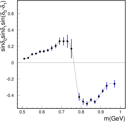
Figure 32: The factor $\sin\delta_{0}\,\sin\delta_{1}\,\sin(\delta_{0}-\delta_{1})$ obtained from $\pi\pi$ phase shifts (figure from [131]).

In the case of two-pion production, $\delta_{0}$ and $\delta_{1}$ can be obtained from the data on $\pi\pi$ phase shifts [148]. The factor $\sin\delta_{0}\,\sin\delta_{1}\,\sin(\delta_{0}-\delta_{1})$ is shown in Fig. 32. It is interesting to observe that the experimental value of this quantity reaches 75% of its theoretical maximum.

6.9 Leptoproduction of spin-1 hadrons

As first suggested by Ji [149] (see also [150]) the transversity distribution can be also probed in leptoproduction of vector mesons (e.g., $\rho,K^{*},\phi$). The fragmentation process into spin-1 hadrons has been fully analysed, from a formal viewpoint, in [151, 152]. The polarisation state of a spin-1 particle is described by a spin vector $\textstyle S$ and by a rank-2 spin tensor $T^{ij}$. The latter contains five parameters, usually called $S_{LL}$, $S_{LT}^{x}$, $S_{LT}^{y}$, $S_{TT}^{xy}$ and $S_{TT}^{xx}$ [151]. The transversity distribution $\Delta_{T}{f}$ emerges when an unpolarised beam strikes a transversely polarised target. The cross-section in this case is [151] (we retain only the terms containing $\Delta_{T}{f}$ and we use the notation of Sec. 6.5.2)

$$\frac{\d\sigma(\mathchoice{\mbox{\boldmath$\displaystyle S$\unboldmath}}{\mbox{\boldmath$\textstyle S$\unboldmath}}{\mbox{\boldmath$\scriptstyle S$\unboldmath}}{\mbox{\boldmath$\scriptscriptstyle S$\unboldmath}}_{\perp})}{\d{x}\d{y}\d{z}\d^{2}\mathchoice{\mbox{\boldmath$\displaystyle P$\unboldmath}}{\mbox{\boldmath$\textstyle P$\unboldmath}}{\mbox{\boldmath$\scriptstyle P$\unboldmath}}{\mbox{\boldmath$\scriptscriptstyle P$\unboldmath}}_{h\perp}}=\frac{4\pi\alpha_{\text{em}}^{2}s}{Q^{4}}\,|\mathchoice{\mbox{\boldmath$\displaystyle S$\unboldmath}}{\mbox{\boldmath$\textstyle S$\unboldmath}}{\mbox{\boldmath$\scriptstyle S$\unboldmath}}{\mbox{\boldmath$\scriptscriptstyle S$\unboldmath}}_{\perp}|\,\sum_{a}e_{a}^{2}\,x(1-y)$$

$$\hbox{}\hskip 14.22636pt\times\left\{\rule[-7.3194pt]{0.0pt}{20.23602pt}|S_{LT}|\,\sin(\phi_{LT}+\phi_{S})\,I[\Delta_{T}{f}_{a}\,H_{1LT}^{a}]\right.$$

$$\hbox{}\hskip 14.22636pt+|S_{TT}|\,\sin(2\phi_{TT}+\phi_{S}-\phi_{h})\,I\left[\frac{\hat{\mathchoice{\mbox{\boldmath$\displaystyle h$\unboldmath}}{\mbox{\boldmath$\textstyle h$\unboldmath}}{\mbox{\boldmath$\scriptstyle h$\unboldmath}}{\mbox{\boldmath$\scriptscriptstyle h$\unboldmath}}}\cdot\mathchoice{\mbox{\boldmath$\displaystyle\kappa$\unboldmath}}{\mbox{\boldmath$\textstyle\kappa$\unboldmath}}{\mbox{\boldmath$\scriptstyle\kappa$\unboldmath}}{\mbox{\boldmath$\scriptscriptstyle\kappa$\unboldmath}}_{\perp}}{M_{h}}\,\Delta_{T}{f}_{a}\,H_{1TT}^{a}\right]$$

$$\hbox{}\hskip 14.22636pt+S_{LL}\,\sin(\phi_{S}+\phi_{h})\,I\left[\frac{\hat{\mathchoice{\mbox{\boldmath$\displaystyle h$\unboldmath}}{\mbox{\boldmath$\textstyle h$\unboldmath}}{\mbox{\boldmath$\scriptstyle h$\unboldmath}}{\mbox{\boldmath$\scriptscriptstyle h$\unboldmath}}}\cdot\mathchoice{\mbox{\boldmath$\displaystyle\kappa$\unboldmath}}{\mbox{\boldmath$\textstyle\kappa$\unboldmath}}{\mbox{\boldmath$\scriptstyle\kappa$\unboldmath}}{\mbox{\boldmath$\scriptscriptstyle\kappa$\unboldmath}}_{\perp}}{M_{h}}\,\Delta_{T}{f}_{a}\,H_{1LL}^{\perp a}\right]$$

$$\hbox{}\hskip 14.22636pt+|S_{LT}|\,\sin(\phi_{LT}-\phi_{S}-2\phi_{h})\,I\left[\frac{2\,(\hat{\mathchoice{\mbox{\boldmath$\displaystyle h$\unboldmath}}{\mbox{\boldmath$\textstyle h$\unboldmath}}{\mbox{\boldmath$\scriptstyle h$\unboldmath}}{\mbox{\boldmath$\scriptscriptstyle h$\unboldmath}}}\cdot\mathchoice{\mbox{\boldmath$\displaystyle\kappa$\unboldmath}}{\mbox{\boldmath$\textstyle\kappa$\unboldmath}}{\mbox{\boldmath$\scriptstyle\kappa$\unboldmath}}{\mbox{\boldmath$\scriptscriptstyle\kappa$\unboldmath}}_{\perp})^{2}-\mathchoice{\mbox{\boldmath$\displaystyle\kappa$\unboldmath}}{\mbox{\boldmath$\textstyle\kappa$\unboldmath}}{\mbox{\boldmath$\scriptstyle\kappa$\unboldmath}}{\mbox{\boldmath$\scriptscriptstyle\kappa$\unboldmath}}_{\perp}^{2}}{2M_{h}^{2}}\,\Delta_{T}{f}_{a}\,H_{1LT}^{\perp a}\right]$$

$$\hbox{}\hskip 14.22636pt-|S_{TT}|\,\sin(2\phi_{TT}-\phi_{S}-3\phi_{h})$$

$$\hbox{}\hskip 28.45274pt\times\left.I\left[\frac{(\hat{\mathchoice{\mbox{\boldmath$\displaystyle h$\unboldmath}}{\mbox{\boldmath$\textstyle h$\unboldmath}}{\mbox{\boldmath$\scriptstyle h$\unboldmath}}{\mbox{\boldmath$\scriptscriptstyle h$\unboldmath}}}\cdot\mathchoice{\mbox{\boldmath$\displaystyle\kappa$\unboldmath}}{\mbox{\boldmath$\textstyle\kappa$\unboldmath}}{\mbox{\boldmath$\scriptstyle\kappa$\unboldmath}}{\mbox{\boldmath$\scriptscriptstyle\kappa$\unboldmath}}_{\perp})\,[2\,(\hat{\mathchoice{\mbox{\boldmath$\displaystyle h$\unboldmath}}{\mbox{\boldmath$\textstyle h$\unboldmath}}{\mbox{\boldmath$\scriptstyle h$\unboldmath}}{\mbox{\boldmath$\scriptscriptstyle h$\unboldmath}}}\cdot\mathchoice{\mbox{\boldmath$\displaystyle\kappa$\unboldmath}}{\mbox{\boldmath$\textstyle\kappa$\unboldmath}}{\mbox{\boldmath$\scriptstyle\kappa$\unboldmath}}{\mbox{\boldmath$\scriptscriptstyle\kappa$\unboldmath}}_{\perp})^{2}-3\mathchoice{\mbox{\boldmath$\displaystyle\kappa$\unboldmath}}{\mbox{\boldmath$\textstyle\kappa$\unboldmath}}{\mbox{\boldmath$\scriptstyle\kappa$\unboldmath}}{\mbox{\boldmath$\scriptscriptstyle\kappa$\unboldmath}}_{\perp}^{2}/2]}{M_{h}^{3}}\,\Delta_{T}{f}_{a}\,H_{1TT}^{\perp a}\right]\rule[-7.3194pt]{0.0pt}{20.23602pt}\right\}+\ldots\,.$$ (6.9.1)

For simplicity, we have omitted the subscript $h$ in the tensor spin parameters (which are understood to pertain to the produced hadron). The azimuthal angles $\phi_{LT}$ and $\phi_{TT}$ are defined by

$$\tan\phi_{LT}=\frac{S_{LT}^{y}}{S_{LT}^{x}}\;,\quad\tan\phi_{TT}=\frac{S_{TT}^{xy}}{S_{TT}^{xx}}\,,$$ (6.9.2)

and

$$|S_{LT}|=\sqrt{(S_{LT}^{x})^{2}+(S_{LT}^{y})^{2}}\;,\quad|S_{TT}|=\sqrt{(S_{TT}^{xx})^{2}+(S_{TT}^{xy})^{2}}\,.$$ (6.9.3)

Note that $\Delta_{T}{f}$ couples in (6.9.1) to five different fragmentation functions: $H_{1LT}$, $H_{1TT}$, $H_{1LL}^{\perp}$, $H_{1LT}^{\perp}$, $H_{1TT}^{\perp}$. All these functions are $T$-odd. If we integrate the cross-section over $\mathchoice{\mbox{\boldmath$\displaystyle P$\unboldmath}}{\mbox{\boldmath$\textstyle P$\unboldmath}}{\mbox{\boldmath$\scriptstyle P$\unboldmath}}{\mbox{\boldmath$\scriptscriptstyle P$\unboldmath}}_{h\perp}$, only one term survives, namely

$$\frac{\d\sigma(\mathchoice{\mbox{\boldmath$\displaystyle S$\unboldmath}}{\mbox{\boldmath$\textstyle S$\unboldmath}}{\mbox{\boldmath$\scriptstyle S$\unboldmath}}{\mbox{\boldmath$\scriptscriptstyle S$\unboldmath}}_{\perp})}{\d{x}\d{y}\d{z}} = \frac{4\pi\alpha_{\text{em}}^{2}s}{Q^{4}}\,|\mathchoice{\mbox{\boldmath$\displaystyle S$\unboldmath}}{\mbox{\boldmath$\textstyle S$\unboldmath}}{\mbox{\boldmath$\scriptstyle S$\unboldmath}}{\mbox{\boldmath$\scriptscriptstyle S$\unboldmath}}_{\perp}|\,|S_{LT}|\sin(\phi_{LT}+\phi_{S})$$ (6.9.4)

$$\hbox{}\times\sum_{a}e_{a}^{2}\,x(1-y)\,\Delta_{T}{f}_{a}(x)\,H_{1LT}^{a}(z)\,.$$

The fragmentation function appearing here, $H_{1LT}$, is called $\hat{h}_{\bar{1}}$ by Ji [149]. It is a $T$-odd and chirally-odd function which can be measured at leading twist and without considering intrinsic transverse momenta. Probing the transversity by (6.9.4) requires polarimetry on the produced meson. For a self-analysing particle this can be done by studying the angular distribution of its decay products (e.g., $\rho^{0}\to\pi^{+}\pi^{-}$). Thus, the vector-meson fragmentation function $H_{1LT}$ represents a specific contribution to two-particle production near the vector meson mass.

6.10 Transversity in exclusive leptoproduction processes

Let us now consider the possibility of observing the transversity distributions in exclusive leptoproduction processes. Collins, Frankfurt and Strikman [153] remarked that the exclusive production of a transversely polarised vector meson in DIS, that is $lp\to{l}Vp$, involves the chirally-odd off-diagonal parton distributions in the proton. These distributions (also called “skewed” or “off-forward” distributions) depend on two variables $x$ and $x^{\prime}$ since the incoming and outgoing proton states have different momenta $P$ and $P^{\prime}$, with $(P^{\prime}-P)^{2}=t$ (the reader may consult [154, 155, 156] on skewed distributions). For instance, the off-forward transversity distribution (represented in Fig. 33a) contains a matrix element of the form $\langle{PS}|\mathchoice{\makebox[0.0pt][l]{$\displaystyle\kern 2.08334pt\overline{\kern-2.43059pt\phantom{\psi}}$}}{\makebox[0.0pt][l]{$\textstyle\kern 2.08334pt\overline{\kern-2.43059pt\phantom{\psi}}$}}{\makebox[0.0pt][l]{$\scriptstyle\kern 1.45834pt\overline{\kern-1.7014pt\phantom{\psi}}$}}{\makebox[0.0pt][l]{$\scriptscriptstyle\kern 1.04167pt\overline{\kern-1.21529pt\phantom{\psi}}$}}\psi(0)\gamma^{+}\gamma_{\perp}\gamma_{5}\psi(\xi^{-})|P^{\prime}S\rangle$. At low $x$ the difference between $x$ and $x^{\prime}$ is small and the off-diagonal distributions are completely determined by the corresponding diagonal ones.

In [157] it was shown that the chirally-odd contribution to vector-meson production (see Fig. 33b) is actually zero at LO in $\alpha_{s}$. This result was later extended in [158], where it was observed that the vanishing of the chirally-odd contribution is due to angular momentum and chirality conservation in the hard scattering and hence holds at leading twist to all orders in the strong coupling. Thus, the (off-diagonal) transversity distributions cannot be probed in exclusive vector-meson leptoproduction.

Figure 33: The off-diagonal transversity distribution (a) and its contribution to exclusive vector meson production (b).

7 Transversity in hadronic reactions

The second class of reactions probing quark transversity is hadron scattering with at least one of the two colliding particles in a transverse polarisation state. We shall first consider the case where both initial hadrons are transversely polarised. In particular, Drell–Yan production with two transversely polarised hadrons turns out to be the most favourable reaction for studying the transversity distributions. Indeed, the pioneering work of Ralston and Soper [9] and Pire and Ralston [159] concentrated precisely on this process. We shall then see how transversity may emerge even when only one of the colliding hadrons is transversely polarised. This possibility, however, is more uncertain.

7.1 Double-spin transverse asymmetries

When both hadrons are transversely polarised, the typical observables are double-spin transverse asymmetries of the form

$$A_{TT}=\frac{\d\sigma(\mathchoice{\mbox{\boldmath$\displaystyle S$\unboldmath}}{\mbox{\boldmath$\textstyle S$\unboldmath}}{\mbox{\boldmath$\scriptstyle S$\unboldmath}}{\mbox{\boldmath$\scriptscriptstyle S$\unboldmath}}_{T},\mathchoice{\mbox{\boldmath$\displaystyle S$\unboldmath}}{\mbox{\boldmath$\textstyle S$\unboldmath}}{\mbox{\boldmath$\scriptstyle S$\unboldmath}}{\mbox{\boldmath$\scriptscriptstyle S$\unboldmath}}_{T})-\d\sigma(\mathchoice{\mbox{\boldmath$\displaystyle S$\unboldmath}}{\mbox{\boldmath$\textstyle S$\unboldmath}}{\mbox{\boldmath$\scriptstyle S$\unboldmath}}{\mbox{\boldmath$\scriptscriptstyle S$\unboldmath}}_{T},-\mathchoice{\mbox{\boldmath$\displaystyle S$\unboldmath}}{\mbox{\boldmath$\textstyle S$\unboldmath}}{\mbox{\boldmath$\scriptstyle S$\unboldmath}}{\mbox{\boldmath$\scriptscriptstyle S$\unboldmath}}_{T})}{\d\sigma(\mathchoice{\mbox{\boldmath$\displaystyle S$\unboldmath}}{\mbox{\boldmath$\textstyle S$\unboldmath}}{\mbox{\boldmath$\scriptstyle S$\unboldmath}}{\mbox{\boldmath$\scriptscriptstyle S$\unboldmath}}_{T},\mathchoice{\mbox{\boldmath$\displaystyle S$\unboldmath}}{\mbox{\boldmath$\textstyle S$\unboldmath}}{\mbox{\boldmath$\scriptstyle S$\unboldmath}}{\mbox{\boldmath$\scriptscriptstyle S$\unboldmath}}_{T})+\d\sigma(\mathchoice{\mbox{\boldmath$\displaystyle S$\unboldmath}}{\mbox{\boldmath$\textstyle S$\unboldmath}}{\mbox{\boldmath$\scriptstyle S$\unboldmath}}{\mbox{\boldmath$\scriptscriptstyle S$\unboldmath}}_{T},-\mathchoice{\mbox{\boldmath$\displaystyle S$\unboldmath}}{\mbox{\boldmath$\textstyle S$\unboldmath}}{\mbox{\boldmath$\scriptstyle S$\unboldmath}}{\mbox{\boldmath$\scriptscriptstyle S$\unboldmath}}_{T})}\,,$$ (7.1.1)

Since there is no gluon transversity distribution for spin-half hadrons, transversely polarised $pp$ reactions which are dominated at the partonic level by $qg$ or $gg$ scattering are expected to yield a very small $A_{TT}$ [21, 160]. Thus, direct-photon production (with lowest-order subprocesses $gq\to{q}\gamma$ and $q\mathchoice{\makebox[0.0pt][l]{$\displaystyle\kern 1.29167pt\overline{\kern-1.50696pt\phantom{q}}$}}{\makebox[0.0pt][l]{$\textstyle\kern 1.29167pt\overline{\kern-1.50696pt\phantom{q}}$}}{\makebox[0.0pt][l]{$\scriptstyle\kern 0.90417pt\overline{\kern-1.05487pt\phantom{q}}$}}{\makebox[0.0pt][l]{$\scriptscriptstyle\kern 0.64583pt\overline{\kern-0.75348pt\phantom{q}}$}}q\to{\gamma}g$), heavy-quark production ($q\mathchoice{\makebox[0.0pt][l]{$\displaystyle\kern 1.29167pt\overline{\kern-1.50696pt\phantom{q}}$}}{\makebox[0.0pt][l]{$\textstyle\kern 1.29167pt\overline{\kern-1.50696pt\phantom{q}}$}}{\makebox[0.0pt][l]{$\scriptstyle\kern 0.90417pt\overline{\kern-1.05487pt\phantom{q}}$}}{\makebox[0.0pt][l]{$\scriptscriptstyle\kern 0.64583pt\overline{\kern-0.75348pt\phantom{q}}$}}q\to{Q}\mathchoice{\makebox[0.0pt][l]{$\displaystyle\kern 2.05pt\overline{\kern-2.3917pt\phantom{Q}}$}}{\makebox[0.0pt][l]{$\textstyle\kern 2.05pt\overline{\kern-2.3917pt\phantom{Q}}$}}{\makebox[0.0pt][l]{$\scriptstyle\kern 1.435pt\overline{\kern-1.67418pt\phantom{Q}}$}}{\makebox[0.0pt][l]{$\scriptscriptstyle\kern 1.025pt\overline{\kern-1.19585pt\phantom{Q}}$}}Q$ and $gg\to{Q}\mathchoice{\makebox[0.0pt][l]{$\displaystyle\kern 2.05pt\overline{\kern-2.3917pt\phantom{Q}}$}}{\makebox[0.0pt][l]{$\textstyle\kern 2.05pt\overline{\kern-2.3917pt\phantom{Q}}$}}{\makebox[0.0pt][l]{$\scriptstyle\kern 1.435pt\overline{\kern-1.67418pt\phantom{Q}}$}}{\makebox[0.0pt][l]{$\scriptscriptstyle\kern 1.025pt\overline{\kern-1.19585pt\phantom{Q}}$}}Q$), and two-gluon-jet production ($gg\to{gg}$ and $q\mathchoice{\makebox[0.0pt][l]{$\displaystyle\kern 1.29167pt\overline{\kern-1.50696pt\phantom{q}}$}}{\makebox[0.0pt][l]{$\textstyle\kern 1.29167pt\overline{\kern-1.50696pt\phantom{q}}$}}{\makebox[0.0pt][l]{$\scriptstyle\kern 0.90417pt\overline{\kern-1.05487pt\phantom{q}}$}}{\makebox[0.0pt][l]{$\scriptscriptstyle\kern 0.64583pt\overline{\kern-0.75348pt\phantom{q}}$}}q\to{gg}$) do not seem to be promising reactions to detect quark transverse polarisation.

The only good candidate process for measuring transversity in doubly polarised $pp$ (or $p\mathchoice{\makebox[0.0pt][l]{$\displaystyle\kern 1.29167pt\overline{\kern-1.50696pt\phantom{p}}$}}{\makebox[0.0pt][l]{$\textstyle\kern 1.29167pt\overline{\kern-1.50696pt\phantom{p}}$}}{\makebox[0.0pt][l]{$\scriptstyle\kern 0.90417pt\overline{\kern-1.05487pt\phantom{p}}$}}{\makebox[0.0pt][l]{$\scriptscriptstyle\kern 0.64583pt\overline{\kern-0.75348pt\phantom{p}}$}}p$) collisions is Drell–Yan lepton pair production [9, 28, 14]. We shall see that at lowest order $A_{TT}^{\text{DY}}$ contains combinations of the products

$$\Delta_{T}{f}(x_{A})\;\Delta_{T}\mathchoice{\makebox[0.0pt][l]{$\displaystyle\kern 2.08334pt\overline{\kern-2.43059pt\phantom{f}}$}}{\makebox[0.0pt][l]{$\textstyle\kern 2.08334pt\overline{\kern-2.43059pt\phantom{f}}$}}{\makebox[0.0pt][l]{$\scriptstyle\kern 1.45834pt\overline{\kern-1.7014pt\phantom{f}}$}}{\makebox[0.0pt][l]{$\scriptscriptstyle\kern 1.04167pt\overline{\kern-1.21529pt\phantom{f}}$}}f(x_{B})\,.$$

The advantage of studying quark transverse polarisation via Drell–Yan is twofold: i) transversity distributions appear at leading-twist level; ii) the cross-section contains no unknown quantities, besides the transversity distributions themselves. This renders theoretical predictions relatively easier, with respect to other reactions.

7.2 The Drell–Yan process

Drell–Yan lepton-pair production is the process

$$A\,(P_{1})\,+\,B\,(P_{2})\to l^{+}\,(\ell)\,+\,l^{-}\,(\ell^{\prime})\,+\,X\,,$$ (7.2.1)

where $A$ and $B$ are protons or antiprotons and $X$ is the undetected hadronic system. The centre-of-mass energy squared of this reaction is $s=(P_{1}+P_{2})^{2}\simeq 2\,P_{1}{\cdot}P_{2}$ (in the following, the hadron masses $M_{1}$ and $M_{2}$ will be systematically neglected, unless otherwise stated). The lepton pair originates from a virtual photon (or from a $Z^{0}$) with four-momentum $q=\ell+\ell^{\prime}$. Note that, in contrast to DIS, $q$ is a time-like vector: $Q^{2}=q^{2}>0$. This is also the invariant mass of the lepton pair. We shall consider the deeply inelastic limit where $Q^{2},s\to\infty$, while the ratio $\tau=Q^{2}/s$ is fixed and finite.

Figure 34: Drell–Yan dilepton production.

The Drell-Yan (DY) cross-section is

$$\d\sigma=\frac{8\pi^{2}\alpha_{\text{em}}^{2}}{s\,Q^{4}}\,2L_{\mu\nu}W^{\mu\nu}\,(2\pi)^{4}\,\frac{\d^{3}\mathchoice{\mbox{\boldmath$\displaystyle\ell$\unboldmath}}{\mbox{\boldmath$\textstyle\ell$\unboldmath}}{\mbox{\boldmath$\scriptstyle\ell$\unboldmath}}{\mbox{\boldmath$\scriptscriptstyle\ell$\unboldmath}}}{(2\pi)^{3}\,2E}\,\frac{\d^{3}\mathchoice{\mbox{\boldmath$\displaystyle\ell$\unboldmath}}{\mbox{\boldmath$\textstyle\ell$\unboldmath}}{\mbox{\boldmath$\scriptstyle\ell$\unboldmath}}{\mbox{\boldmath$\scriptscriptstyle\ell$\unboldmath}}^{\prime}}{(2\pi)^{3}\,2E^{\prime}}\,,$$ (7.2.2)

where the leptonic tensor, neglecting lepton masses and ignoring their polarisation, is given by

$$L_{\mu\nu}=2\left(\ell_{\mu}\ell^{\prime}_{\nu}+\ell_{\nu}\ell^{\prime}_{\mu}-\frac{Q^{2}}{2}\,g_{\mu\nu}\right),$$ (7.2.3)

and the hadronic tensor is defined as

$$W^{\mu\nu} = \frac{1}{(2\pi)^{4}}\,\sum_{X}\int\!\frac{\d^{3}\mathchoice{\mbox{\boldmath$\displaystyle P$\unboldmath}}{\mbox{\boldmath$\textstyle P$\unboldmath}}{\mbox{\boldmath$\scriptstyle P$\unboldmath}}{\mbox{\boldmath$\scriptscriptstyle P$\unboldmath}}_{X}}{(2\pi)^{3}\,2E_{X}}\,(2\pi)^{4}\,\delta^{4}(P_{1}+P_{2}-q-P_{X})$$ (7.2.4)

$$\hbox{}\times\langle P_{1}S_{1},P_{2}S_{2}|J^{\mu}(0)|X\rangle\langle X|J^{\nu}(0)|P_{1}S_{1},P_{2}S_{2}\rangle$$

$$= \frac{1}{(2\pi)^{4}}\int\!\d^{4}\xi\,\e^{\text{i}q{\cdot}\xi}\,\langle P_{1}S_{1},P_{2}S_{2}|J^{\mu}(z)J^{\nu}(0)|P_{1}S_{1},P_{2}S_{2}\rangle\,.$$

The phase space in (7.2.2) can be rewritten as

$$\frac{\d^{3}\mathchoice{\mbox{\boldmath$\displaystyle\ell$\unboldmath}}{\mbox{\boldmath$\textstyle\ell$\unboldmath}}{\mbox{\boldmath$\scriptstyle\ell$\unboldmath}}{\mbox{\boldmath$\scriptscriptstyle\ell$\unboldmath}}}{(2\pi)^{3}\,2E}\,\frac{\d^{3}\mathchoice{\mbox{\boldmath$\displaystyle\ell$\unboldmath}}{\mbox{\boldmath$\textstyle\ell$\unboldmath}}{\mbox{\boldmath$\scriptstyle\ell$\unboldmath}}{\mbox{\boldmath$\scriptscriptstyle\ell$\unboldmath}}^{\prime}}{(2\pi)^{3}\,2E^{\prime}}=\frac{\d\Omega\,\d^{4}q}{8(2\pi)^{6}}\,,$$ (7.2.5)

where $\Omega$ is the solid angle identifying the direction of the leptons in their rest frame. Using (7.2.5) the DY cross-section takes the form

$$\frac{\d\sigma}{\d^{4}q\,\d\Omega}=\frac{\alpha_{\text{em}}^{2}}{2s\,Q^{4}}\,L_{\mu\nu}W^{\mu\nu}\,.$$ (7.2.6)

We define now the two invariants

$$x_{1}=\frac{Q^{2}}{2P_{1}{\cdot}q}\,,\qquad x_{2}=\frac{Q^{2}}{2P_{2}{\cdot}q}\,.$$ (7.2.7)

In the parton model $x_{1}$ and $x_{2}$ will be interpreted as the fractions of the longitudinal momenta of the hadrons $A$ and $B$ carried by the quark and the antiquark which annihilate into the virtual photon.

In a frame where the two colliding hadrons are collinear ($A$ is taken to move in the positive $z$ direction), the photon momentum can be parametrised as

$$q^{\mu}=\frac{Q^{2}}{x_{2}s}\,P_{1}^{\mu}+\frac{Q^{2}}{x_{1}s}\,P_{2}^{\mu}+q_{T}^{\mu}\,.$$ (7.2.8)

Neglecting terms of order $\mathop{\mathcal{O}}\nolimits(1/Q^{2})$, one finds $Q^{2}/x_{1}x_{2}s\simeq 1$, that is $\tau=Q^{2}/s=x_{1}x_{2}$, and therefore

$$q^{\mu}=x_{1}\,P_{1}^{\mu}+x_{2}\,P_{2}^{\mu}+q_{T}^{\mu}=\left[x_{1}\,P_{1}^{+},x_{2}\,P_{2}^{-},\mathchoice{\mbox{\boldmath$\displaystyle q$\unboldmath}}{\mbox{\boldmath$\textstyle q$\unboldmath}}{\mbox{\boldmath$\scriptstyle q$\unboldmath}}{\mbox{\boldmath$\scriptscriptstyle q$\unboldmath}}_{T}\right].$$ (7.2.9)

Note that

$$x_{1}\simeq\frac{P_{2}{\cdot}q}{P_{1}{\cdot}P_{2}}\,,\qquad x_{2}\simeq\frac{P_{1}{\cdot}q}{P_{1}{\cdot}P_{2}}\,.$$ (7.2.10)

In terms of $x_{1}$, $x_{2}$ and $\mathchoice{\mbox{\boldmath$\displaystyle q$\unboldmath}}{\mbox{\boldmath$\textstyle q$\unboldmath}}{\mbox{\boldmath$\scriptstyle q$\unboldmath}}{\mbox{\boldmath$\scriptscriptstyle q$\unboldmath}}_{T}$ the DY cross-section reads

$$\frac{\d\sigma}{\d{x}_{1}\,\d{x}_{2}\,\d^{2}\mathchoice{\mbox{\boldmath$\displaystyle q$\unboldmath}}{\mbox{\boldmath$\textstyle q$\unboldmath}}{\mbox{\boldmath$\scriptstyle q$\unboldmath}}{\mbox{\boldmath$\scriptscriptstyle q$\unboldmath}}_{T}\,\d\Omega}=\frac{\alpha_{\text{em}}^{2}}{4Q^{4}}\,L_{\mu\nu}W^{\mu\nu}\,.$$ (7.2.11)

It is customary [9, 161] to introduce three vectors $Z^{\mu}$, $X^{\mu}$ and $Y^{\mu}$ defined as

$$Z^{\mu} = \frac{P_{2}{\cdot}q}{P_{1}{\cdot}P_{2}}\,P_{1}^{\mu}-\frac{P_{1}{\cdot}q}{P_{1}{\cdot}P_{2}}\,P_{2}^{\mu}\,,$$ (7.2.12a)

$$X^{\mu} = -\frac{1}{P_{1}{\cdot}P_{2}}\left[P_{2}{\cdot}Z\,\widetilde{P}_{1}^{\mu}-P_{1}{\cdot}Z\,\widetilde{P}_{2}^{\mu}\right],$$ (7.2.12b)

$$Y^{\mu} = \frac{1}{P_{1}{\cdot}P_{2}}\,\varepsilon^{\mu\nu\rho\sigma}\,P_{1\nu}P_{2\rho}q_{\sigma}\,.$$ (7.2.12c)

where $\widetilde{P}_{1,2}^{\mu}=P_{1,2}^{\mu}-(P_{1,2}{\cdot}q/q^{2})\,q^{\mu}$. These vectors are mutually orthogonal and orthogonal to $q^{\mu}$, and satisfy

$$Z^{2}\simeq-Q^{2}\,,\qquad X^{2}\simeq Y^{2}\simeq-\mathchoice{\mbox{\boldmath$\displaystyle q$\unboldmath}}{\mbox{\boldmath$\textstyle q$\unboldmath}}{\mbox{\boldmath$\scriptstyle q$\unboldmath}}{\mbox{\boldmath$\scriptscriptstyle q$\unboldmath}}_{T}^{2}\,.$$ (7.2.13)

Thus, they form a set of spacelike axes and have only spatial components in the dilepton rest frame. Using (7.2.9), $Z^{\mu}$, $X^{\mu}$ and $Y^{\mu}$ can be expressed as

$$Z^{\mu}=x_{1}\,P_{1}^{\mu}-x_{2}\,P_{2}^{\mu}\,,\qquad X^{\mu}=q_{T}^{\mu}\,,\qquad Y^{\mu}=\varepsilon_{T}^{\sigma\mu}\,q_{T\sigma}\,,$$ (7.2.14)

where

$$\varepsilon_{T}^{\sigma\mu}\equiv\frac{1}{P_{1}{\cdot}P_{2}}\,\varepsilon^{\sigma\mu\nu\rho}P_{1\nu}P_{2\rho}\,.$$ (7.2.15)

In terms of the unit vectors

$$\hat{x}^{\mu}=\frac{X^{\mu}}{\sqrt{-X^{2}}}\,,\quad\hat{y}^{\mu}=\frac{Y^{\mu}}{\sqrt{-Y^{2}}}\,,\quad\hat{z}^{\mu}=\frac{Z^{\mu}}{\sqrt{-Z^{2}}}\,,\quad\hat{q}^{\mu}=\frac{q^{\mu}}{\sqrt{Q^{2}}}\,,$$ (7.2.16)

the lepton momenta can be expanded as

$$\ell^{\mu} = {\textstyle\frac{1}{2}}\,q^{\mu}+{\textstyle\frac{1}{2}}\,Q\,(\sin\theta\,\cos\phi\,\hat{x}^{\mu}+\sin\theta\,\sin\phi\,\hat{y}^{\mu}+\cos\theta\,\hat{z}^{\mu})\,,$$ (7.2.17a)

$${\ell^{\prime}}^{\mu} = {\textstyle\frac{1}{2}}\,q^{\mu}-{\textstyle\frac{1}{2}}\,Q\,(\sin\theta\,\cos\phi\,\hat{x}^{\mu}+\sin\theta\,\sin\phi\,\hat{y}^{\mu}+\cos\theta\,\hat{z}^{\mu})\,.$$ (7.2.17b)

The geometry of the process in the dilepton rest frame is shown in Fig. 35.

Figure 35: The geometry of Drell–Yan production in the rest frame of the lepton pair.

The leptonic tensor then reads

$$L^{\mu\nu} = -{\textstyle\frac{1}{2}}Q^{2}\left[(1+\cos^{2}\theta)\,g_{\perp}^{\mu\nu}-2\sin^{2}\theta\,\hat{z}^{\mu}\hat{\zeta}^{\nu}\right.$$ (7.2.18)

$$\hskip 25.00003pt\hbox{}+2\sin^{2}\theta\,\cos 2\phi\,(\hat{x}^{\mu}\hat{x}^{\nu}+{\textstyle\frac{1}{2}}g_{\perp}^{\mu\nu})+\sin^{2}\theta\,\sin 2\phi\;\hat{x}^{\{\mu}\hat{y}^{\nu\}}$$

$$\hskip 25.00003pt\hbox{}\left.+\sin 2\theta\,\cos\phi\;\hat{z}^{\{\mu}\hat{x}^{\nu\}}+\sin 2\theta\,\sin\phi\;\hat{z}^{\{\mu}\hat{y}^{\nu\}}\right],$$

where

$$g_{\perp}^{\mu\nu}=g^{\mu\nu}-\hat{q}^{\mu}\hat{q}^{\nu}+\hat{z}^{\mu}\hat{z}^{\nu}.$$ (7.2.19)

In the parton model, calling $k$ and $k^{\prime}$ the momenta of the quark (or antiquark) coming from hadron $A$ and $B$ respectively, the hadronic tensor is (see Fig. 36)

$$W^{\mu\nu}=\frac{1}{3}\,\sum_{a}e_{a}^{2}\int\!\frac{\d^{4}k}{(2\pi)^{4}}\int\!\frac{\d^{4}k^{\prime}}{(2\pi)^{4}}\,\delta^{4}(k+k^{\prime}-q)\,\mathop{\text{Tr}}\nolimits[\Phi_{1}\,\gamma^{\mu}\,\mathchoice{\makebox[0.0pt][l]{$\displaystyle\kern 2.05pt\overline{\kern-2.3917pt\phantom{\Phi}}$}}{\makebox[0.0pt][l]{$\textstyle\kern 2.05pt\overline{\kern-2.3917pt\phantom{\Phi}}$}}{\makebox[0.0pt][l]{$\scriptstyle\kern 1.435pt\overline{\kern-1.67418pt\phantom{\Phi}}$}}{\makebox[0.0pt][l]{$\scriptscriptstyle\kern 1.025pt\overline{\kern-1.19585pt\phantom{\Phi}}$}}\Phi_{2}\gamma^{\nu}].$$ (7.2.20)

Here $\Phi_{1}$ is the quark correlation matrix for hadron $A$, eq. (4.1.1), $\mathchoice{\makebox[0.0pt][l]{$\displaystyle\kern 2.05pt\overline{\kern-2.3917pt\phantom{\Phi}}$}}{\makebox[0.0pt][l]{$\textstyle\kern 2.05pt\overline{\kern-2.3917pt\phantom{\Phi}}$}}{\makebox[0.0pt][l]{$\scriptstyle\kern 1.435pt\overline{\kern-1.67418pt\phantom{\Phi}}$}}{\makebox[0.0pt][l]{$\scriptscriptstyle\kern 1.025pt\overline{\kern-1.19585pt\phantom{\Phi}}$}}\Phi_{2}$ is the antiquark correlation matrix for hadron $B$, eq. (4.2.9), and the factor $1/3$ has been added since in $\Phi_{1}$ and $\mathchoice{\makebox[0.0pt][l]{$\displaystyle\kern 2.05pt\overline{\kern-2.3917pt\phantom{\Phi}}$}}{\makebox[0.0pt][l]{$\textstyle\kern 2.05pt\overline{\kern-2.3917pt\phantom{\Phi}}$}}{\makebox[0.0pt][l]{$\scriptstyle\kern 1.435pt\overline{\kern-1.67418pt\phantom{\Phi}}$}}{\makebox[0.0pt][l]{$\scriptscriptstyle\kern 1.025pt\overline{\kern-1.19585pt\phantom{\Phi}}$}}\Phi_{2}$ summations over colours are implicit. It is understood that, in order to obtain the complete expression of the hadronic tensor, one must add to (7.2.20) a term with $\Phi_{1}$ replaced by $\Phi_{2}$ and $\mathchoice{\makebox[0.0pt][l]{$\displaystyle\kern 2.05pt\overline{\kern-2.3917pt\phantom{\Phi}}$}}{\makebox[0.0pt][l]{$\textstyle\kern 2.05pt\overline{\kern-2.3917pt\phantom{\Phi}}$}}{\makebox[0.0pt][l]{$\scriptstyle\kern 1.435pt\overline{\kern-1.67418pt\phantom{\Phi}}$}}{\makebox[0.0pt][l]{$\scriptscriptstyle\kern 1.025pt\overline{\kern-1.19585pt\phantom{\Phi}}$}}\Phi_{2}$ replaced by $\mathchoice{\makebox[0.0pt][l]{$\displaystyle\kern 2.05pt\overline{\kern-2.3917pt\phantom{\Phi}}$}}{\makebox[0.0pt][l]{$\textstyle\kern 2.05pt\overline{\kern-2.3917pt\phantom{\Phi}}$}}{\makebox[0.0pt][l]{$\scriptstyle\kern 1.435pt\overline{\kern-1.67418pt\phantom{\Phi}}$}}{\makebox[0.0pt][l]{$\scriptscriptstyle\kern 1.025pt\overline{\kern-1.19585pt\phantom{\Phi}}$}}\Phi_{1}$, which accounts for the case where a quark is extracted from $B$ and an antiquark is extracted from $A$. In the following formulæ we shall denote this term symbolically by $[1\leftrightarrow 2]$.

Figure 36: The parton-model diagram for the Drell–Yan hadronic tensor.

Hereafter the quark transverse motion (which is discussed at length in [161]) will be ignored and only the ordinary collinear configuration will be considered.

We now evaluate the hadronic tensor in a frame where $A$ and $B$ move collinearly, with large longitudinal momentum. Setting $k\simeq\xi_{1}\,P_{1}$, $k^{\prime}\simeq\xi_{2}\,P_{2}$ and using (7.2.9), the delta function in (7.2.20) gives

$$\delta^{4}(k+k^{\prime}-\kappa) = \delta(k^{+}+{k^{\prime}}^{+}-q^{+})\,\delta(k^{-}+{k^{\prime}}^{-}-q^{-})\,\delta^{2}(\mathchoice{\mbox{\boldmath$\displaystyle q$\unboldmath}}{\mbox{\boldmath$\textstyle q$\unboldmath}}{\mbox{\boldmath$\scriptstyle q$\unboldmath}}{\mbox{\boldmath$\scriptscriptstyle q$\unboldmath}}_{T})$$ (7.2.21)

$$\simeq \delta(\xi_{1}P_{1}^{+}-x_{1}P_{1}^{+})\,\delta(\xi_{2}P_{2}^{-}-x_{2}P_{2}^{-})\,\delta^{2}(\mathchoice{\mbox{\boldmath$\displaystyle q$\unboldmath}}{\mbox{\boldmath$\textstyle q$\unboldmath}}{\mbox{\boldmath$\scriptstyle q$\unboldmath}}{\mbox{\boldmath$\scriptscriptstyle q$\unboldmath}}_{T})$$

$$= \frac{1}{P_{1}^{+}\,P_{2}^{-}}\,\delta(\xi_{1}-x_{1})\,\delta(\xi_{2}-x_{2})\,\delta^{2}(\mathchoice{\mbox{\boldmath$\displaystyle q$\unboldmath}}{\mbox{\boldmath$\textstyle q$\unboldmath}}{\mbox{\boldmath$\scriptstyle q$\unboldmath}}{\mbox{\boldmath$\scriptscriptstyle q$\unboldmath}}_{T})\,.$$

The hadronic tensor then becomes

$$W^{\mu\nu} = \frac{1}{3}\,\sum_{a}e_{a}^{2}\int\!\frac{\d{k}^{-}\,\d^{2}\mathchoice{\mbox{\boldmath$\displaystyle k$\unboldmath}}{\mbox{\boldmath$\textstyle k$\unboldmath}}{\mbox{\boldmath$\scriptstyle k$\unboldmath}}{\mbox{\boldmath$\scriptscriptstyle k$\unboldmath}}_{T}}{(2\pi)^{4}}\int\!\frac{\d{k^{\prime}}^{+}\,\d^{2}\mathchoice{\mbox{\boldmath$\displaystyle k$\unboldmath}}{\mbox{\boldmath$\textstyle k$\unboldmath}}{\mbox{\boldmath$\scriptstyle k$\unboldmath}}{\mbox{\boldmath$\scriptscriptstyle k$\unboldmath}}_{T}^{\prime}}{(2\pi)^{4}}\,\delta^{2}(\mathchoice{\mbox{\boldmath$\displaystyle q$\unboldmath}}{\mbox{\boldmath$\textstyle q$\unboldmath}}{\mbox{\boldmath$\scriptstyle q$\unboldmath}}{\mbox{\boldmath$\scriptscriptstyle q$\unboldmath}}_{T})$$ (7.2.22)

$$\hskip 25.00003pt\hbox{}\times\mathop{\text{Tr}}\nolimits[\Phi_{1}\,\gamma^{\mu}\,\mathchoice{\makebox[0.0pt][l]{$\displaystyle\kern 2.05pt\overline{\kern-2.3917pt\phantom{\Phi}}$}}{\makebox[0.0pt][l]{$\textstyle\kern 2.05pt\overline{\kern-2.3917pt\phantom{\Phi}}$}}{\makebox[0.0pt][l]{$\scriptstyle\kern 1.435pt\overline{\kern-1.67418pt\phantom{\Phi}}$}}{\makebox[0.0pt][l]{$\scriptscriptstyle\kern 1.025pt\overline{\kern-1.19585pt\phantom{\Phi}}$}}\Phi_{2}\gamma^{\nu}]_{k^{+}=x_{1}P_{1}^{+},\,{k^{\prime}}^{-}=x_{2}P_{2}^{-}}+[1\leftrightarrow 2]\,.$$

Since the leptonic tensor is symmetric, only the symmetric part of $W^{\mu\nu}$ contributes to the cross-section. For $\mathop{\text{Tr}}\nolimits[\Phi_{1}\gamma^{\{\mu}\mathchoice{\makebox[0.0pt][l]{$\displaystyle\kern 2.05pt\overline{\kern-2.3917pt\phantom{\Phi}}$}}{\makebox[0.0pt][l]{$\textstyle\kern 2.05pt\overline{\kern-2.3917pt\phantom{\Phi}}$}}{\makebox[0.0pt][l]{$\scriptstyle\kern 1.435pt\overline{\kern-1.67418pt\phantom{\Phi}}$}}{\makebox[0.0pt][l]{$\scriptscriptstyle\kern 1.025pt\overline{\kern-1.19585pt\phantom{\Phi}}$}}\Phi_{2}\gamma^{\nu\}}]$ we resort to the Fierz decomposition (6.5.2), with the replacements $\Phi\to\Phi_{1}$, $\Xi\to\mathchoice{\makebox[0.0pt][l]{$\displaystyle\kern 2.05pt\overline{\kern-2.3917pt\phantom{\Phi}}$}}{\makebox[0.0pt][l]{$\textstyle\kern 2.05pt\overline{\kern-2.3917pt\phantom{\Phi}}$}}{\makebox[0.0pt][l]{$\scriptstyle\kern 1.435pt\overline{\kern-1.67418pt\phantom{\Phi}}$}}{\makebox[0.0pt][l]{$\scriptscriptstyle\kern 1.025pt\overline{\kern-1.19585pt\phantom{\Phi}}$}}\Phi_{2}$. Using (4.2.5a–LABEL:subdf18) and (4.2.12–4.2.14), we then obtain (the spins of the two hadrons are $\mathchoice{\mbox{\boldmath$\displaystyle S$\unboldmath}}{\mbox{\boldmath$\textstyle S$\unboldmath}}{\mbox{\boldmath$\scriptstyle S$\unboldmath}}{\mbox{\boldmath$\scriptscriptstyle S$\unboldmath}}_{1}=(\mathchoice{\mbox{\boldmath$\displaystyle S$\unboldmath}}{\mbox{\boldmath$\textstyle S$\unboldmath}}{\mbox{\boldmath$\scriptstyle S$\unboldmath}}{\mbox{\boldmath$\scriptscriptstyle S$\unboldmath}}_{1T},\lambda_{1})$ and $\mathchoice{\mbox{\boldmath$\displaystyle S$\unboldmath}}{\mbox{\boldmath$\textstyle S$\unboldmath}}{\mbox{\boldmath$\scriptstyle S$\unboldmath}}{\mbox{\boldmath$\scriptscriptstyle S$\unboldmath}}_{2}=(\mathchoice{\mbox{\boldmath$\displaystyle S$\unboldmath}}{\mbox{\boldmath$\textstyle S$\unboldmath}}{\mbox{\boldmath$\scriptstyle S$\unboldmath}}{\mbox{\boldmath$\scriptscriptstyle S$\unboldmath}}_{2T},\lambda_{2})$)

$$\int\!\d^{2}\mathchoice{\mbox{\boldmath$\displaystyle q$\unboldmath}}{\mbox{\boldmath$\textstyle q$\unboldmath}}{\mbox{\boldmath$\scriptstyle q$\unboldmath}}{\mbox{\boldmath$\scriptscriptstyle q$\unboldmath}}_{T}\,W^{\mu\nu} = \frac{1}{3}\sum_{a}e_{a}^{2}\left\{-g_{T}^{\mu\nu}\left[f_{a}(x_{1})\,\mathchoice{\makebox[0.0pt][l]{$\displaystyle\kern 2.08334pt\overline{\kern-2.43059pt\phantom{f}}$}}{\makebox[0.0pt][l]{$\textstyle\kern 2.08334pt\overline{\kern-2.43059pt\phantom{f}}$}}{\makebox[0.0pt][l]{$\scriptstyle\kern 1.45834pt\overline{\kern-1.7014pt\phantom{f}}$}}{\makebox[0.0pt][l]{$\scriptscriptstyle\kern 1.04167pt\overline{\kern-1.21529pt\phantom{f}}$}}f_{a}(x_{2})+\lambda_{1}\lambda_{2}\,\Delta{f}_{a}(x_{1})\,\Delta\mathchoice{\makebox[0.0pt][l]{$\displaystyle\kern 2.08334pt\overline{\kern-2.43059pt\phantom{f}}$}}{\makebox[0.0pt][l]{$\textstyle\kern 2.08334pt\overline{\kern-2.43059pt\phantom{f}}$}}{\makebox[0.0pt][l]{$\scriptstyle\kern 1.45834pt\overline{\kern-1.7014pt\phantom{f}}$}}{\makebox[0.0pt][l]{$\scriptscriptstyle\kern 1.04167pt\overline{\kern-1.21529pt\phantom{f}}$}}f_{a}(x_{2})\right]\right.$$ (7.2.23)

$$\hbox{}-\left.\left[S_{1T}^{\{\mu}S_{2T}^{\nu\}}+\mathchoice{\mbox{\boldmath$\displaystyle S$\unboldmath}}{\mbox{\boldmath$\textstyle S$\unboldmath}}{\mbox{\boldmath$\scriptstyle S$\unboldmath}}{\mbox{\boldmath$\scriptscriptstyle S$\unboldmath}}_{1T}{\cdot}\mathchoice{\mbox{\boldmath$\displaystyle S$\unboldmath}}{\mbox{\boldmath$\textstyle S$\unboldmath}}{\mbox{\boldmath$\scriptstyle S$\unboldmath}}{\mbox{\boldmath$\scriptscriptstyle S$\unboldmath}}_{2T}\,g_{T}^{\mu\nu}\right]\Delta_{T}{f}_{a}(x_{1})\,\Delta_{T}\mathchoice{\makebox[0.0pt][l]{$\displaystyle\kern 2.08334pt\overline{\kern-2.43059pt\phantom{f}}$}}{\makebox[0.0pt][l]{$\textstyle\kern 2.08334pt\overline{\kern-2.43059pt\phantom{f}}$}}{\makebox[0.0pt][l]{$\scriptstyle\kern 1.45834pt\overline{\kern-1.7014pt\phantom{f}}$}}{\makebox[0.0pt][l]{$\scriptscriptstyle\kern 1.04167pt\overline{\kern-1.21529pt\phantom{f}}$}}f_{a}(x_{2})\right\}$$

$$\hbox{}+[1\leftrightarrow 2]\,.$$

In contracting the leptonic and the hadronic tensors, it is convenient to pass from the $AB$ collinear frame to the $\gamma^{*}A$ collinear frame. We recall that, at leading twist, the transverse ($T$) vectors approximately coincide with the vectors perpendicular to the photon direction (denoted by a subscript $\perp$): $\mathchoice{\mbox{\boldmath$\displaystyle S$\unboldmath}}{\mbox{\boldmath$\textstyle S$\unboldmath}}{\mbox{\boldmath$\scriptstyle S$\unboldmath}}{\mbox{\boldmath$\scriptscriptstyle S$\unboldmath}}_{1T}\simeq\mathchoice{\mbox{\boldmath$\displaystyle S$\unboldmath}}{\mbox{\boldmath$\textstyle S$\unboldmath}}{\mbox{\boldmath$\scriptstyle S$\unboldmath}}{\mbox{\boldmath$\scriptscriptstyle S$\unboldmath}}_{1\perp}$, $\mathchoice{\mbox{\boldmath$\displaystyle S$\unboldmath}}{\mbox{\boldmath$\textstyle S$\unboldmath}}{\mbox{\boldmath$\scriptstyle S$\unboldmath}}{\mbox{\boldmath$\scriptscriptstyle S$\unboldmath}}_{2T}\simeq\mathchoice{\mbox{\boldmath$\displaystyle S$\unboldmath}}{\mbox{\boldmath$\textstyle S$\unboldmath}}{\mbox{\boldmath$\scriptstyle S$\unboldmath}}{\mbox{\boldmath$\scriptscriptstyle S$\unboldmath}}_{2\perp}$, $g_{T}^{\mu\nu}\simeq{}g_{\perp}^{\mu\nu}$. Therefore, the contraction $L_{\mu\nu}\,W^{\mu\nu}$ can be performed by means of the following identities

$$-g_{\perp}^{\mu\nu}L_{\mu\nu} = Q^{2}(1+\cos^{2}\theta),$$ (7.2.24a)

$$\left[S_{1\perp}^{\{\mu}S_{2\perp}^{\nu\}}+\mathchoice{\mbox{\boldmath$\displaystyle S$\unboldmath}}{\mbox{\boldmath$\textstyle S$\unboldmath}}{\mbox{\boldmath$\scriptstyle S$\unboldmath}}{\mbox{\boldmath$\scriptscriptstyle S$\unboldmath}}_{1\perp}{\cdot}\mathchoice{\mbox{\boldmath$\displaystyle S$\unboldmath}}{\mbox{\boldmath$\textstyle S$\unboldmath}}{\mbox{\boldmath$\scriptstyle S$\unboldmath}}{\mbox{\boldmath$\scriptscriptstyle S$\unboldmath}}_{2\perp}\,g_{\perp}^{\mu\nu}\right]L_{\mu\nu} =$$ (7.2.24b)

$$\hbox{}-Q^{2}\sin^{2}\theta|\mathchoice{\mbox{\boldmath$\displaystyle S$\unboldmath}}{\mbox{\boldmath$\textstyle S$\unboldmath}}{\mbox{\boldmath$\scriptstyle S$\unboldmath}}{\mbox{\boldmath$\scriptscriptstyle S$\unboldmath}}_{1\perp}||\mathchoice{\mbox{\boldmath$\displaystyle S$\unboldmath}}{\mbox{\boldmath$\textstyle S$\unboldmath}}{\mbox{\boldmath$\scriptstyle S$\unboldmath}}{\mbox{\boldmath$\scriptscriptstyle S$\unboldmath}}_{2\perp}|\cos(2\phi-\phi_{S_{1}}-\phi_{S_{2}})\,,$$

where $\theta$ is the polar angle of the lepton pair in the dilepton rest frame and $\phi_{S_{1}}$ ($\phi_{S_{2}}$) is the azimuthal angle of $\mathchoice{\mbox{\boldmath$\displaystyle S$\unboldmath}}{\mbox{\boldmath$\textstyle S$\unboldmath}}{\mbox{\boldmath$\scriptstyle S$\unboldmath}}{\mbox{\boldmath$\scriptscriptstyle S$\unboldmath}}_{1\perp}$ ($\mathchoice{\mbox{\boldmath$\displaystyle S$\unboldmath}}{\mbox{\boldmath$\textstyle S$\unboldmath}}{\mbox{\boldmath$\scriptstyle S$\unboldmath}}{\mbox{\boldmath$\scriptscriptstyle S$\unboldmath}}_{2\perp}$), measured with respect to the lepton plane. For the Drell–Yan cross-section we finally obtain

$$\frac{\d\sigma}{\d\Omega\d{x}_{1}\d{x}_{2}} = \frac{\alpha_{\text{em}}^{2}}{4Q^{2}}\,\sum_{a}\,\frac{e_{a}^{2}}{3}\left\{\left[f_{a}(x_{1})\,\mathchoice{\makebox[0.0pt][l]{$\displaystyle\kern 2.08334pt\overline{\kern-2.43059pt\phantom{f}}$}}{\makebox[0.0pt][l]{$\textstyle\kern 2.08334pt\overline{\kern-2.43059pt\phantom{f}}$}}{\makebox[0.0pt][l]{$\scriptstyle\kern 1.45834pt\overline{\kern-1.7014pt\phantom{f}}$}}{\makebox[0.0pt][l]{$\scriptscriptstyle\kern 1.04167pt\overline{\kern-1.21529pt\phantom{f}}$}}f_{a}(x_{2})\right.\right.$$ (7.2.25)

$$\hbox{}+\left.\lambda_{1}\,\lambda_{2}\,\Delta{f}_{a}(x_{1})\,\Delta\mathchoice{\makebox[0.0pt][l]{$\displaystyle\kern 2.08334pt\overline{\kern-2.43059pt\phantom{f}}$}}{\makebox[0.0pt][l]{$\textstyle\kern 2.08334pt\overline{\kern-2.43059pt\phantom{f}}$}}{\makebox[0.0pt][l]{$\scriptstyle\kern 1.45834pt\overline{\kern-1.7014pt\phantom{f}}$}}{\makebox[0.0pt][l]{$\scriptscriptstyle\kern 1.04167pt\overline{\kern-1.21529pt\phantom{f}}$}}f_{a}(x_{2})\right](1+\cos^{2}\theta)$$

$$\hbox{}+\left.|\mathchoice{\mbox{\boldmath$\displaystyle S$\unboldmath}}{\mbox{\boldmath$\textstyle S$\unboldmath}}{\mbox{\boldmath$\scriptstyle S$\unboldmath}}{\mbox{\boldmath$\scriptscriptstyle S$\unboldmath}}_{1\perp}|\,|\mathchoice{\mbox{\boldmath$\displaystyle S$\unboldmath}}{\mbox{\boldmath$\textstyle S$\unboldmath}}{\mbox{\boldmath$\scriptstyle S$\unboldmath}}{\mbox{\boldmath$\scriptscriptstyle S$\unboldmath}}_{2\perp}|\,\cos(2\phi-\phi_{S_{1}}-\phi_{S_{2}})\,\Delta_{T}{f}_{a}(x_{1})\,\Delta_{T}\mathchoice{\makebox[0.0pt][l]{$\displaystyle\kern 2.08334pt\overline{\kern-2.43059pt\phantom{f}}$}}{\makebox[0.0pt][l]{$\textstyle\kern 2.08334pt\overline{\kern-2.43059pt\phantom{f}}$}}{\makebox[0.0pt][l]{$\scriptstyle\kern 1.45834pt\overline{\kern-1.7014pt\phantom{f}}$}}{\makebox[0.0pt][l]{$\scriptscriptstyle\kern 1.04167pt\overline{\kern-1.21529pt\phantom{f}}$}}f_{a}(x_{2})\,\sin^{2}\theta\right\}$$

$$\hbox{}+[1\leftrightarrow 2]\,.$$

From this we derive the parton-model expression for the double transverse asymmetry:

$$A_{TT}^{\text{DY}} = \frac{\d\sigma(\mathchoice{\mbox{\boldmath$\displaystyle S$\unboldmath}}{\mbox{\boldmath$\textstyle S$\unboldmath}}{\mbox{\boldmath$\scriptstyle S$\unboldmath}}{\mbox{\boldmath$\scriptscriptstyle S$\unboldmath}}_{1\perp},\mathchoice{\mbox{\boldmath$\displaystyle S$\unboldmath}}{\mbox{\boldmath$\textstyle S$\unboldmath}}{\mbox{\boldmath$\scriptstyle S$\unboldmath}}{\mbox{\boldmath$\scriptscriptstyle S$\unboldmath}}_{2\perp})-\d\sigma(\mathchoice{\mbox{\boldmath$\displaystyle S$\unboldmath}}{\mbox{\boldmath$\textstyle S$\unboldmath}}{\mbox{\boldmath$\scriptstyle S$\unboldmath}}{\mbox{\boldmath$\scriptscriptstyle S$\unboldmath}}_{1\perp},-\mathchoice{\mbox{\boldmath$\displaystyle S$\unboldmath}}{\mbox{\boldmath$\textstyle S$\unboldmath}}{\mbox{\boldmath$\scriptstyle S$\unboldmath}}{\mbox{\boldmath$\scriptscriptstyle S$\unboldmath}}_{2\perp})}{\d\sigma(\mathchoice{\mbox{\boldmath$\displaystyle S$\unboldmath}}{\mbox{\boldmath$\textstyle S$\unboldmath}}{\mbox{\boldmath$\scriptstyle S$\unboldmath}}{\mbox{\boldmath$\scriptscriptstyle S$\unboldmath}}_{1\perp},\mathchoice{\mbox{\boldmath$\displaystyle S$\unboldmath}}{\mbox{\boldmath$\textstyle S$\unboldmath}}{\mbox{\boldmath$\scriptstyle S$\unboldmath}}{\mbox{\boldmath$\scriptscriptstyle S$\unboldmath}}_{2\perp})+\d\sigma(\mathchoice{\mbox{\boldmath$\displaystyle S$\unboldmath}}{\mbox{\boldmath$\textstyle S$\unboldmath}}{\mbox{\boldmath$\scriptstyle S$\unboldmath}}{\mbox{\boldmath$\scriptscriptstyle S$\unboldmath}}_{1\perp},-\mathchoice{\mbox{\boldmath$\displaystyle S$\unboldmath}}{\mbox{\boldmath$\textstyle S$\unboldmath}}{\mbox{\boldmath$\scriptstyle S$\unboldmath}}{\mbox{\boldmath$\scriptscriptstyle S$\unboldmath}}_{2\perp})}$$ (7.2.26)

$$= |\mathchoice{\mbox{\boldmath$\displaystyle S$\unboldmath}}{\mbox{\boldmath$\textstyle S$\unboldmath}}{\mbox{\boldmath$\scriptstyle S$\unboldmath}}{\mbox{\boldmath$\scriptscriptstyle S$\unboldmath}}_{1\perp}||\mathchoice{\mbox{\boldmath$\displaystyle S$\unboldmath}}{\mbox{\boldmath$\textstyle S$\unboldmath}}{\mbox{\boldmath$\scriptstyle S$\unboldmath}}{\mbox{\boldmath$\scriptscriptstyle S$\unboldmath}}_{2\perp}|\,\frac{\sin^{2}\theta\,\cos(2\phi-\phi_{S_{1}}-\phi_{S_{2}})}{1+\cos^{2}\theta}$$

$$\hbox{}\times\frac{\sum_{a}e_{a}^{2}\,\Delta_{T}{f}_{a}(x_{1})\Delta_{T}\mathchoice{\makebox[0.0pt][l]{$\displaystyle\kern 2.08334pt\overline{\kern-2.43059pt\phantom{f}}$}}{\makebox[0.0pt][l]{$\textstyle\kern 2.08334pt\overline{\kern-2.43059pt\phantom{f}}$}}{\makebox[0.0pt][l]{$\scriptstyle\kern 1.45834pt\overline{\kern-1.7014pt\phantom{f}}$}}{\makebox[0.0pt][l]{$\scriptscriptstyle\kern 1.04167pt\overline{\kern-1.21529pt\phantom{f}}$}}f_{a}(x_{2})+[1\leftrightarrow 2]}{\sum_{a}e_{a}^{2}\,f_{a}(x_{1})\mathchoice{\makebox[0.0pt][l]{$\displaystyle\kern 2.08334pt\overline{\kern-2.43059pt\phantom{f}}$}}{\makebox[0.0pt][l]{$\textstyle\kern 2.08334pt\overline{\kern-2.43059pt\phantom{f}}$}}{\makebox[0.0pt][l]{$\scriptstyle\kern 1.45834pt\overline{\kern-1.7014pt\phantom{f}}$}}{\makebox[0.0pt][l]{$\scriptscriptstyle\kern 1.04167pt\overline{\kern-1.21529pt\phantom{f}}$}}f_{a}(x_{2})+[1\leftrightarrow 2]}\,,$$

and we see that a measurement of $A_{TT}^{\text{DY}}$ directly provides the product of quark and antiquark transverse polarisation distributions $\Delta_{T}{f}(x_{1})\,\Delta_{T}{f}(x_{2})$, with no mixing with other unknown quantities. Thus, the Drell–Yan process seems to be, at least in principle, a very good reaction to probe transversity. Note that in leading-order QCD, eq. (7.2.26) is still valid, with $Q^{2}$ dependent distribution functions, namely

$$A_{TT}^{\text{DY}} = |\mathchoice{\mbox{\boldmath$\displaystyle S$\unboldmath}}{\mbox{\boldmath$\textstyle S$\unboldmath}}{\mbox{\boldmath$\scriptstyle S$\unboldmath}}{\mbox{\boldmath$\scriptscriptstyle S$\unboldmath}}_{1\perp}||\mathchoice{\mbox{\boldmath$\displaystyle S$\unboldmath}}{\mbox{\boldmath$\textstyle S$\unboldmath}}{\mbox{\boldmath$\scriptstyle S$\unboldmath}}{\mbox{\boldmath$\scriptscriptstyle S$\unboldmath}}_{2\perp}|\,\frac{\sin^{2}\theta\,\cos(2\phi-\phi_{S_{1}}-\phi_{S_{2}})}{1+\cos^{2}\theta}$$ (7.2.27)

$$\hbox{}\times\frac{\sum_{a}e_{a}^{2}\,\Delta_{T}{f}_{a}(x_{1},Q^{2})\Delta_{T}\mathchoice{\makebox[0.0pt][l]{$\displaystyle\kern 2.08334pt\overline{\kern-2.43059pt\phantom{f}}$}}{\makebox[0.0pt][l]{$\textstyle\kern 2.08334pt\overline{\kern-2.43059pt\phantom{f}}$}}{\makebox[0.0pt][l]{$\scriptstyle\kern 1.45834pt\overline{\kern-1.7014pt\phantom{f}}$}}{\makebox[0.0pt][l]{$\scriptscriptstyle\kern 1.04167pt\overline{\kern-1.21529pt\phantom{f}}$}}f_{a}(x_{2},Q^{2})+[1\leftrightarrow 2]}{\sum_{a}e_{a}^{2}\,f_{a}(x_{1},Q^{2})\mathchoice{\makebox[0.0pt][l]{$\displaystyle\kern 2.08334pt\overline{\kern-2.43059pt\phantom{f}}$}}{\makebox[0.0pt][l]{$\textstyle\kern 2.08334pt\overline{\kern-2.43059pt\phantom{f}}$}}{\makebox[0.0pt][l]{$\scriptstyle\kern 1.45834pt\overline{\kern-1.7014pt\phantom{f}}$}}{\makebox[0.0pt][l]{$\scriptscriptstyle\kern 1.04167pt\overline{\kern-1.21529pt\phantom{f}}$}}f_{a}(x_{2},Q^{2})+[1\leftrightarrow 2]}\,.$$

Here $\Delta_{T}{f}(x,Q^{2})$ are the transversity distributions evolved at LO. In Sec. 9.1 we shall see some predictions for $A_{TT}^{\text{DY}}$.

7.2.1 $Z^{0}$-mediated Drell–Yan process

If Drell–Yan dilepton production is mediated by the exchange of a $Z^{0}$ boson, the vertex $e_{i}\,\gamma^{\mu}$, where $e_{i}$ is the electric charge of particle $i$ (quark or lepton), is replaced by $(V_{i}+A_{i}\,\gamma_{5})\,\gamma^{\mu}$, where the vector and axial-vector couplings are

$$\begin{split}V_{i}&=T_{3}^{i}-2e_{i}\,\sin^{2}\vartheta_{W}\,,\\ A_{i}&=T_{3}^{i}\,.\end{split}$$ (7.2.28)

The weak isospin $T_{3}^{i}$ is $+{\textstyle\frac{1}{2}}$ for $i=u$ and $-{\textstyle\frac{1}{2}}$ for $i=l^{-},d,s$.

The resulting double transverse asymmetry has a form similar to (7.2.26), with the necessary changes in the couplings. Omitting the interference contributions, it reads

$$A_{TT}^{\text{DY},Z} = |\mathchoice{\mbox{\boldmath$\displaystyle S$\unboldmath}}{\mbox{\boldmath$\textstyle S$\unboldmath}}{\mbox{\boldmath$\scriptstyle S$\unboldmath}}{\mbox{\boldmath$\scriptscriptstyle S$\unboldmath}}_{1\perp}||\mathchoice{\mbox{\boldmath$\displaystyle S$\unboldmath}}{\mbox{\boldmath$\textstyle S$\unboldmath}}{\mbox{\boldmath$\scriptstyle S$\unboldmath}}{\mbox{\boldmath$\scriptscriptstyle S$\unboldmath}}_{2\perp}|\,\frac{\sin^{2}\theta\,\cos(2\phi-\phi_{S_{1}}-\phi_{S_{2}})}{1+\cos^{2}\theta}$$ (7.2.29)

$$\hbox{}\times\frac{\sum_{a}(V_{a}^{2}-A_{a}^{2})\,\Delta_{T}{f}_{a}(x_{1})\Delta_{T}\mathchoice{\makebox[0.0pt][l]{$\displaystyle\kern 2.08334pt\overline{\kern-2.43059pt\phantom{f}}$}}{\makebox[0.0pt][l]{$\textstyle\kern 2.08334pt\overline{\kern-2.43059pt\phantom{f}}$}}{\makebox[0.0pt][l]{$\scriptstyle\kern 1.45834pt\overline{\kern-1.7014pt\phantom{f}}$}}{\makebox[0.0pt][l]{$\scriptscriptstyle\kern 1.04167pt\overline{\kern-1.21529pt\phantom{f}}$}}f_{a}(x_{2})+[1\leftrightarrow 2]}{\sum_{a}(V_{a}^{2}+A_{a}^{2})\,f_{a}(x_{1})\mathchoice{\makebox[0.0pt][l]{$\displaystyle\kern 2.08334pt\overline{\kern-2.43059pt\phantom{f}}$}}{\makebox[0.0pt][l]{$\textstyle\kern 2.08334pt\overline{\kern-2.43059pt\phantom{f}}$}}{\makebox[0.0pt][l]{$\scriptstyle\kern 1.45834pt\overline{\kern-1.7014pt\phantom{f}}$}}{\makebox[0.0pt][l]{$\scriptscriptstyle\kern 1.04167pt\overline{\kern-1.21529pt\phantom{f}}$}}f_{a}(x_{2})+[1\leftrightarrow 2]}\,.$$

7.3 Factorisation in Drell–Yan processes

With a view to extending the results previously obtained to NLO in QCD, we now rederive them in the framework of QCD factorisation [144]. The Drell–Yan cross-section is written in a factorised form as (hereafter we omit the exchanged term $[1\leftrightarrow 2]$)

$$\d\sigma = \sum_{a}\sum_{\alpha\alpha^{\prime}\beta\beta^{\prime}}\int\!\d\xi_{1}\int\!\d\xi_{2}\;\rho_{\alpha^{\prime}\alpha}^{(1)}\,f_{a}(\xi_{1},\mu^{2})\,\rho_{\beta^{\prime}\beta}^{(2)}\,\mathchoice{\makebox[0.0pt][l]{$\displaystyle\kern 2.08334pt\overline{\kern-2.43059pt\phantom{f}}$}}{\makebox[0.0pt][l]{$\textstyle\kern 2.08334pt\overline{\kern-2.43059pt\phantom{f}}$}}{\makebox[0.0pt][l]{$\scriptstyle\kern 1.45834pt\overline{\kern-1.7014pt\phantom{f}}$}}{\makebox[0.0pt][l]{$\scriptscriptstyle\kern 1.04167pt\overline{\kern-1.21529pt\phantom{f}}$}}f_{a}(\xi_{2},\mu^{2})$$ (7.3.1)

$$\hskip 80.00012pt\hbox{}\times\left[\d\hat{\sigma}(Q^{2}/\mu^{2},\alpha_{s}(\mu^{2}))\right]_{\alpha\alpha^{\prime}\beta\beta^{\prime}}\,,$$

where $\xi_{1}$ and $\xi_{2}$ are the momentum fractions of the quark (from hadron $A$) and antiquark (from $B$), $\rho^{(1)}$ and $\rho^{(2)}$ are the quark and antiquark spin density matrices, and $(\d\hat{\sigma})_{\alpha\alpha^{\prime}\beta\beta^{\prime}}$ is the cross-section matrix (in the quark and antiquark spin space) of the elementary subprocesses. As usual, $\mu$ denotes the factorisation scale.

At LO $\d\hat{\sigma}$ incorporates a delta function of energy–momentum conservation, namely $\delta^{4}(k+k^{\prime}-q)$, which sets $\xi_{1}=x_{1}$, $\xi_{2}=x_{2}$ and $\mathchoice{\mbox{\boldmath$\displaystyle q$\unboldmath}}{\mbox{\boldmath$\textstyle q$\unboldmath}}{\mbox{\boldmath$\scriptstyle q$\unboldmath}}{\mbox{\boldmath$\scriptscriptstyle q$\unboldmath}}_{T}=0$. Thus eq. (7.3.1) becomes (omitting the scales)

$$\frac{\d\sigma}{\d\Omega\d{x}_{1}\d{x}_{2}}=\sum_{a}\sum_{\alpha\alpha^{\prime}\beta\beta^{\prime}}\rho_{\alpha^{\prime}\alpha}^{(1)}\,\rho_{\beta^{\prime}\beta}^{(2)}\left(\frac{\d\hat{\sigma}}{\d\Omega}\right)_{\alpha\alpha^{\prime}\beta\beta^{\prime}}f_{a}(\xi_{1})\,\mathchoice{\makebox[0.0pt][l]{$\displaystyle\kern 2.08334pt\overline{\kern-2.43059pt\phantom{f}}$}}{\makebox[0.0pt][l]{$\textstyle\kern 2.08334pt\overline{\kern-2.43059pt\phantom{f}}$}}{\makebox[0.0pt][l]{$\scriptstyle\kern 1.45834pt\overline{\kern-1.7014pt\phantom{f}}$}}{\makebox[0.0pt][l]{$\scriptscriptstyle\kern 1.04167pt\overline{\kern-1.21529pt\phantom{f}}$}}f_{a}(\xi_{2})\,,$$ (7.3.2)

where the only subprocess is $q\mathchoice{\makebox[0.0pt][l]{$\displaystyle\kern 1.29167pt\overline{\kern-1.50696pt\phantom{q}}$}}{\makebox[0.0pt][l]{$\textstyle\kern 1.29167pt\overline{\kern-1.50696pt\phantom{q}}$}}{\makebox[0.0pt][l]{$\scriptstyle\kern 0.90417pt\overline{\kern-1.05487pt\phantom{q}}$}}{\makebox[0.0pt][l]{$\scriptscriptstyle\kern 0.64583pt\overline{\kern-0.75348pt\phantom{q}}$}}q\to{l^{+}l^{-}}$ (see Fig. 37) and its cross-section is

$$\left(\frac{\d\hat{\sigma}}{\d\Omega}\right)_{\alpha\alpha^{\prime}\beta\beta^{\prime}}=\frac{1}{64\pi^{2}\hat{s}}\,\sum_{\gamma\delta}\mathcal{M}^{*}_{\alpha\beta\gamma\delta}\,\mathcal{M}_{\alpha^{\prime}\beta^{\prime}\gamma\delta}\,.$$ (7.3.3)

Figure 37: The $q\bar{q}\to{}l^{+}l^{-}$ process contributing to Drell–Yan production at LO.

The contributing scattering amplitudes are

$$\mathcal{M}_{++++}=\mathcal{M}_{----}\,,\qquad\mathcal{M}_{++--}=\mathcal{M}_{--++}\,,$$ (7.3.4)

and the cross-section (7.3.2) reduces to

$$\frac{\d\sigma}{\d\Omega\d{x}_{1}\d{x}_{2}} = \sum_{a}\left\{\left(\rho_{++}^{(1)}\rho_{++}^{(2)}+\rho_{--}^{(1)}\rho_{--}^{(2)}\right)\left(\frac{\d\hat{\sigma}}{\d\Omega}\right)_{++++}\right.$$ (7.3.5)

$$\hbox{}+\left.\left(\rho_{+-}^{(1)}\rho_{+-}^{(2)}+\rho_{-+}^{(1)}\rho_{-+}^{(2)}\right)\left(\frac{\d\hat{\sigma}}{\d\Omega}\right)_{+-+-}\right\}f_{a}(x_{1})\,\mathchoice{\makebox[0.0pt][l]{$\displaystyle\kern 2.08334pt\overline{\kern-2.43059pt\phantom{f}}$}}{\makebox[0.0pt][l]{$\textstyle\kern 2.08334pt\overline{\kern-2.43059pt\phantom{f}}$}}{\makebox[0.0pt][l]{$\scriptstyle\kern 1.45834pt\overline{\kern-1.7014pt\phantom{f}}$}}{\makebox[0.0pt][l]{$\scriptscriptstyle\kern 1.04167pt\overline{\kern-1.21529pt\phantom{f}}$}}f_{a}(x_{2})\,.\qquad$$

Here the spin density matrix elements are, for the quark

$$\begin{array}[]{rcl@{\qquad}rcl}\rho_{++}^{(1)}&=&{\textstyle\frac{1}{2}}(1+\lambda)\,,&\rho_{--}^{(1)}&=&{\textstyle\frac{1}{2}}(1-\lambda)\,,\\ \rho_{+-}^{(1)}&=&{\textstyle\frac{1}{2}}(s_{x}-\text{i}\,s_{y})\,,&\rho_{-+}^{(1)}&=&{\textstyle\frac{1}{2}}(s_{x}+\text{i}\,s_{y})\,,\end{array}$$ (7.3.6a)

and for the antiquark

$$\begin{array}[]{rcl@{\qquad}rcl}\rho_{++}^{(2)}&=&{\textstyle\frac{1}{2}}(1+\mathchoice{\makebox[0.0pt][l]{$\displaystyle\kern 2.08334pt\overline{\kern-2.43059pt\phantom{\lambda}}$}}{\makebox[0.0pt][l]{$\textstyle\kern 2.08334pt\overline{\kern-2.43059pt\phantom{\lambda}}$}}{\makebox[0.0pt][l]{$\scriptstyle\kern 1.45834pt\overline{\kern-1.7014pt\phantom{\lambda}}$}}{\makebox[0.0pt][l]{$\scriptscriptstyle\kern 1.04167pt\overline{\kern-1.21529pt\phantom{\lambda}}$}}\lambda)\,,&\rho_{--}^{(2)}&=&{\textstyle\frac{1}{2}}(1-\mathchoice{\makebox[0.0pt][l]{$\displaystyle\kern 2.08334pt\overline{\kern-2.43059pt\phantom{\lambda}}$}}{\makebox[0.0pt][l]{$\textstyle\kern 2.08334pt\overline{\kern-2.43059pt\phantom{\lambda}}$}}{\makebox[0.0pt][l]{$\scriptstyle\kern 1.45834pt\overline{\kern-1.7014pt\phantom{\lambda}}$}}{\makebox[0.0pt][l]{$\scriptscriptstyle\kern 1.04167pt\overline{\kern-1.21529pt\phantom{\lambda}}$}}\lambda)\,,\\ \rho_{+-}^{(2)}&=&{\textstyle\frac{1}{2}}(\mathchoice{\makebox[0.0pt][l]{$\displaystyle\kern 1.29167pt\overline{\kern-1.50696pt\phantom{s}}$}}{\makebox[0.0pt][l]{$\textstyle\kern 1.29167pt\overline{\kern-1.50696pt\phantom{s}}$}}{\makebox[0.0pt][l]{$\scriptstyle\kern 0.90417pt\overline{\kern-1.05487pt\phantom{s}}$}}{\makebox[0.0pt][l]{$\scriptscriptstyle\kern 0.64583pt\overline{\kern-0.75348pt\phantom{s}}$}}s_{x}-\text{i}\,\mathchoice{\makebox[0.0pt][l]{$\displaystyle\kern 1.29167pt\overline{\kern-1.50696pt\phantom{s}}$}}{\makebox[0.0pt][l]{$\textstyle\kern 1.29167pt\overline{\kern-1.50696pt\phantom{s}}$}}{\makebox[0.0pt][l]{$\scriptstyle\kern 0.90417pt\overline{\kern-1.05487pt\phantom{s}}$}}{\makebox[0.0pt][l]{$\scriptscriptstyle\kern 0.64583pt\overline{\kern-0.75348pt\phantom{s}}$}}s_{y})\,,&\rho_{-+}^{(2)}&=&{\textstyle\frac{1}{2}}(\mathchoice{\makebox[0.0pt][l]{$\displaystyle\kern 1.29167pt\overline{\kern-1.50696pt\phantom{s}}$}}{\makebox[0.0pt][l]{$\textstyle\kern 1.29167pt\overline{\kern-1.50696pt\phantom{s}}$}}{\makebox[0.0pt][l]{$\scriptstyle\kern 0.90417pt\overline{\kern-1.05487pt\phantom{s}}$}}{\makebox[0.0pt][l]{$\scriptscriptstyle\kern 0.64583pt\overline{\kern-0.75348pt\phantom{s}}$}}s_{x}+\text{i}\,\mathchoice{\makebox[0.0pt][l]{$\displaystyle\kern 1.29167pt\overline{\kern-1.50696pt\phantom{s}}$}}{\makebox[0.0pt][l]{$\textstyle\kern 1.29167pt\overline{\kern-1.50696pt\phantom{s}}$}}{\makebox[0.0pt][l]{$\scriptstyle\kern 0.90417pt\overline{\kern-1.05487pt\phantom{s}}$}}{\makebox[0.0pt][l]{$\scriptscriptstyle\kern 0.64583pt\overline{\kern-0.75348pt\phantom{s}}$}}s_{y})\,,\end{array}$$ (7.3.6b)

so that (7.3.5) becomes

$$\frac{\d\sigma}{\d\Omega\d{x}_{1}\d{x}_{2}} = \frac{1}{2}\sum_{a}\left\{(1+\lambda\,\mathchoice{\makebox[0.0pt][l]{$\displaystyle\kern 2.08334pt\overline{\kern-2.43059pt\phantom{\lambda}}$}}{\makebox[0.0pt][l]{$\textstyle\kern 2.08334pt\overline{\kern-2.43059pt\phantom{\lambda}}$}}{\makebox[0.0pt][l]{$\scriptstyle\kern 1.45834pt\overline{\kern-1.7014pt\phantom{\lambda}}$}}{\makebox[0.0pt][l]{$\scriptscriptstyle\kern 1.04167pt\overline{\kern-1.21529pt\phantom{\lambda}}$}}\lambda)\left(\frac{\d\hat{\sigma}}{\d\Omega}\right)_{++++}\right.$$ (7.3.7)

$$\hskip 25.00003pt\hbox{}+\left.(s_{x}\,\mathchoice{\makebox[0.0pt][l]{$\displaystyle\kern 1.29167pt\overline{\kern-1.50696pt\phantom{s}}$}}{\makebox[0.0pt][l]{$\textstyle\kern 1.29167pt\overline{\kern-1.50696pt\phantom{s}}$}}{\makebox[0.0pt][l]{$\scriptstyle\kern 0.90417pt\overline{\kern-1.05487pt\phantom{s}}$}}{\makebox[0.0pt][l]{$\scriptscriptstyle\kern 0.64583pt\overline{\kern-0.75348pt\phantom{s}}$}}s_{x}-s_{y}\,\mathchoice{\makebox[0.0pt][l]{$\displaystyle\kern 1.29167pt\overline{\kern-1.50696pt\phantom{s}}$}}{\makebox[0.0pt][l]{$\textstyle\kern 1.29167pt\overline{\kern-1.50696pt\phantom{s}}$}}{\makebox[0.0pt][l]{$\scriptstyle\kern 0.90417pt\overline{\kern-1.05487pt\phantom{s}}$}}{\makebox[0.0pt][l]{$\scriptscriptstyle\kern 0.64583pt\overline{\kern-0.75348pt\phantom{s}}$}}s_{y})\left(\frac{\d\hat{\sigma}}{\d\Omega}\right)_{+-+-}\right\}\,f_{a}(x_{1})\,\mathchoice{\makebox[0.0pt][l]{$\displaystyle\kern 2.08334pt\overline{\kern-2.43059pt\phantom{f}}$}}{\makebox[0.0pt][l]{$\textstyle\kern 2.08334pt\overline{\kern-2.43059pt\phantom{f}}$}}{\makebox[0.0pt][l]{$\scriptstyle\kern 1.45834pt\overline{\kern-1.7014pt\phantom{f}}$}}{\makebox[0.0pt][l]{$\scriptscriptstyle\kern 1.04167pt\overline{\kern-1.21529pt\phantom{f}}$}}f_{a}(x_{2})\,.\qquad$$

At LO, the scattering amplitudes for the $q\mathchoice{\makebox[0.0pt][l]{$\displaystyle\kern 1.29167pt\overline{\kern-1.50696pt\phantom{q}}$}}{\makebox[0.0pt][l]{$\textstyle\kern 1.29167pt\overline{\kern-1.50696pt\phantom{q}}$}}{\makebox[0.0pt][l]{$\scriptstyle\kern 0.90417pt\overline{\kern-1.05487pt\phantom{q}}$}}{\makebox[0.0pt][l]{$\scriptscriptstyle\kern 0.64583pt\overline{\kern-0.75348pt\phantom{q}}$}}q$ annihilation process are

$$\mathcal{M}_{++++}=\mathcal{M}_{----} = e^{2}\,e_{a}\,(1-\cos\theta)\,,$$ (7.3.8a)

$$\mathcal{M}_{++--}=\mathcal{M}_{--++} = e^{2}\,e_{a}\,(1+\cos\theta)\,,$$ (7.3.8b)

and the elementary cross-sections then read

$$\left(\frac{\d\hat{\sigma}}{\d\Omega}\right)_{++++}=\left(\frac{\d\hat{\sigma}}{\d\Omega}\right)_{----} = \frac{1}{64\pi^{2}\hat{s}}\left(|\mathcal{M}_{++++}|^{2}+|\mathcal{M}_{++--}|^{2}\right)$$ (7.3.9a)

$$= \frac{\alpha_{\text{em}}^{2}\,e_{a}^{2}}{2\hat{s}}\,\frac{1}{3}\left(1+\cos^{2}\theta\right),$$

$$\left(\frac{\d\hat{\sigma}}{\d\Omega}\right)_{+-+-}=\left(\frac{\d\hat{\sigma}}{\d\Omega}\right)_{-+-+} = \frac{1}{64\pi^{2}\hat{s}}\,2\mathop{\text{Re}}\nolimits\left(\mathcal{M}^{*}_{++++}\,\mathcal{M}_{++--}\right)$$ (7.3.9b)

$$= \frac{\alpha_{\text{em}}^{2}\,e_{a}^{2}}{2\hat{s}}\,\frac{1}{3}\,\sin^{2}\theta\,.$$

Inserting (7.3.9a, LABEL:subdyfac8) into (7.3.7) we obtain

$$\frac{\d\sigma}{\d\Omega\d{x}_{1}\d{x}_{2}} = \frac{\alpha_{\text{em}}^{2}}{4Q^{2}}\,\sum_{a}\,\frac{e_{a}^{2}}{3}\left\{(1+\lambda\mathchoice{\makebox[0.0pt][l]{$\displaystyle\kern 2.08334pt\overline{\kern-2.43059pt\phantom{\lambda}}$}}{\makebox[0.0pt][l]{$\textstyle\kern 2.08334pt\overline{\kern-2.43059pt\phantom{\lambda}}$}}{\makebox[0.0pt][l]{$\scriptstyle\kern 1.45834pt\overline{\kern-1.7014pt\phantom{\lambda}}$}}{\makebox[0.0pt][l]{$\scriptscriptstyle\kern 1.04167pt\overline{\kern-1.21529pt\phantom{\lambda}}$}}\lambda)\,(1+\cos^{2}\theta)\right.$$ (7.3.10)

$$\hbox{}+\left.(s_{x}\,\mathchoice{\makebox[0.0pt][l]{$\displaystyle\kern 1.29167pt\overline{\kern-1.50696pt\phantom{s}}$}}{\makebox[0.0pt][l]{$\textstyle\kern 1.29167pt\overline{\kern-1.50696pt\phantom{s}}$}}{\makebox[0.0pt][l]{$\scriptstyle\kern 0.90417pt\overline{\kern-1.05487pt\phantom{s}}$}}{\makebox[0.0pt][l]{$\scriptscriptstyle\kern 0.64583pt\overline{\kern-0.75348pt\phantom{s}}$}}s_{x}-s_{y}\,\mathchoice{\makebox[0.0pt][l]{$\displaystyle\kern 1.29167pt\overline{\kern-1.50696pt\phantom{s}}$}}{\makebox[0.0pt][l]{$\textstyle\kern 1.29167pt\overline{\kern-1.50696pt\phantom{s}}$}}{\makebox[0.0pt][l]{$\scriptstyle\kern 0.90417pt\overline{\kern-1.05487pt\phantom{s}}$}}{\makebox[0.0pt][l]{$\scriptscriptstyle\kern 0.64583pt\overline{\kern-0.75348pt\phantom{s}}$}}s_{y})\,\sin^{2}\theta\right\}\,f_{a}(x_{1})\,\mathchoice{\makebox[0.0pt][l]{$\displaystyle\kern 2.08334pt\overline{\kern-2.43059pt\phantom{f}}$}}{\makebox[0.0pt][l]{$\textstyle\kern 2.08334pt\overline{\kern-2.43059pt\phantom{f}}$}}{\makebox[0.0pt][l]{$\scriptstyle\kern 1.45834pt\overline{\kern-1.7014pt\phantom{f}}$}}{\makebox[0.0pt][l]{$\scriptscriptstyle\kern 1.04167pt\overline{\kern-1.21529pt\phantom{f}}$}}f_{a}(x_{2})\,.$$

Using

$$\lambda\,f_{a}(x_{1}) = \lambda_{1}\,\Delta{f}_{a}(x_{1})\,,\qquad\mathchoice{\mbox{\boldmath$\displaystyle s$\unboldmath}}{\mbox{\boldmath$\textstyle s$\unboldmath}}{\mbox{\boldmath$\scriptstyle s$\unboldmath}}{\mbox{\boldmath$\scriptscriptstyle s$\unboldmath}}_{\perp}\,f_{a}(x_{1})=\mathchoice{\mbox{\boldmath$\displaystyle S$\unboldmath}}{\mbox{\boldmath$\textstyle S$\unboldmath}}{\mbox{\boldmath$\scriptstyle S$\unboldmath}}{\mbox{\boldmath$\scriptscriptstyle S$\unboldmath}}_{1\perp}\,\Delta_{T}{f}_{a}(x_{1})\,,$$ (7.3.11a)

$$\mathchoice{\makebox[0.0pt][l]{$\displaystyle\kern 2.08334pt\overline{\kern-2.43059pt\phantom{\lambda}}$}}{\makebox[0.0pt][l]{$\textstyle\kern 2.08334pt\overline{\kern-2.43059pt\phantom{\lambda}}$}}{\makebox[0.0pt][l]{$\scriptstyle\kern 1.45834pt\overline{\kern-1.7014pt\phantom{\lambda}}$}}{\makebox[0.0pt][l]{$\scriptscriptstyle\kern 1.04167pt\overline{\kern-1.21529pt\phantom{\lambda}}$}}\lambda\,\mathchoice{\makebox[0.0pt][l]{$\displaystyle\kern 2.08334pt\overline{\kern-2.43059pt\phantom{f}}$}}{\makebox[0.0pt][l]{$\textstyle\kern 2.08334pt\overline{\kern-2.43059pt\phantom{f}}$}}{\makebox[0.0pt][l]{$\scriptstyle\kern 1.45834pt\overline{\kern-1.7014pt\phantom{f}}$}}{\makebox[0.0pt][l]{$\scriptscriptstyle\kern 1.04167pt\overline{\kern-1.21529pt\phantom{f}}$}}f_{a}(x_{2}) = \lambda_{2}\,\Delta\mathchoice{\makebox[0.0pt][l]{$\displaystyle\kern 2.08334pt\overline{\kern-2.43059pt\phantom{f}}$}}{\makebox[0.0pt][l]{$\textstyle\kern 2.08334pt\overline{\kern-2.43059pt\phantom{f}}$}}{\makebox[0.0pt][l]{$\scriptstyle\kern 1.45834pt\overline{\kern-1.7014pt\phantom{f}}$}}{\makebox[0.0pt][l]{$\scriptscriptstyle\kern 1.04167pt\overline{\kern-1.21529pt\phantom{f}}$}}f_{a}(x_{2})\,,\qquad\mathchoice{\makebox[0.0pt][l]{$\displaystyle\kern 1.29167pt\overline{\kern-1.50696pt\phantom{\mathchoice{\mbox{\boldmath$\displaystyle s$\unboldmath}}{\mbox{\boldmath$\textstyle s$\unboldmath}}{\mbox{\boldmath$\scriptstyle s$\unboldmath}}{\mbox{\boldmath$\scriptscriptstyle s$\unboldmath}}}}$}}{\makebox[0.0pt][l]{$\textstyle\kern 1.29167pt\overline{\kern-1.50696pt\phantom{\mathchoice{\mbox{\boldmath$\displaystyle s$\unboldmath}}{\mbox{\boldmath$\textstyle s$\unboldmath}}{\mbox{\boldmath$\scriptstyle s$\unboldmath}}{\mbox{\boldmath$\scriptscriptstyle s$\unboldmath}}}}$}}{\makebox[0.0pt][l]{$\scriptstyle\kern 0.90417pt\overline{\kern-1.05487pt\phantom{\mathchoice{\mbox{\boldmath$\displaystyle s$\unboldmath}}{\mbox{\boldmath$\textstyle s$\unboldmath}}{\mbox{\boldmath$\scriptstyle s$\unboldmath}}{\mbox{\boldmath$\scriptscriptstyle s$\unboldmath}}}}$}}{\makebox[0.0pt][l]{$\scriptscriptstyle\kern 0.64583pt\overline{\kern-0.75348pt\phantom{\mathchoice{\mbox{\boldmath$\displaystyle s$\unboldmath}}{\mbox{\boldmath$\textstyle s$\unboldmath}}{\mbox{\boldmath$\scriptstyle s$\unboldmath}}{\mbox{\boldmath$\scriptscriptstyle s$\unboldmath}}}}$}}\mathchoice{\mbox{\boldmath$\displaystyle s$\unboldmath}}{\mbox{\boldmath$\textstyle s$\unboldmath}}{\mbox{\boldmath$\scriptstyle s$\unboldmath}}{\mbox{\boldmath$\scriptscriptstyle s$\unboldmath}}_{\perp}\,\mathchoice{\makebox[0.0pt][l]{$\displaystyle\kern 2.08334pt\overline{\kern-2.43059pt\phantom{f}}$}}{\makebox[0.0pt][l]{$\textstyle\kern 2.08334pt\overline{\kern-2.43059pt\phantom{f}}$}}{\makebox[0.0pt][l]{$\scriptstyle\kern 1.45834pt\overline{\kern-1.7014pt\phantom{f}}$}}{\makebox[0.0pt][l]{$\scriptscriptstyle\kern 1.04167pt\overline{\kern-1.21529pt\phantom{f}}$}}f_{a}(x_{2})=\mathchoice{\mbox{\boldmath$\displaystyle S$\unboldmath}}{\mbox{\boldmath$\textstyle S$\unboldmath}}{\mbox{\boldmath$\scriptstyle S$\unboldmath}}{\mbox{\boldmath$\scriptscriptstyle S$\unboldmath}}_{2\perp}\,\Delta_{T}\mathchoice{\makebox[0.0pt][l]{$\displaystyle\kern 2.08334pt\overline{\kern-2.43059pt\phantom{f}}$}}{\makebox[0.0pt][l]{$\textstyle\kern 2.08334pt\overline{\kern-2.43059pt\phantom{f}}$}}{\makebox[0.0pt][l]{$\scriptstyle\kern 1.45834pt\overline{\kern-1.7014pt\phantom{f}}$}}{\makebox[0.0pt][l]{$\scriptscriptstyle\kern 1.04167pt\overline{\kern-1.21529pt\phantom{f}}$}}f_{a}(x_{2})\,,$$ (7.3.11b)

we obtain

$$\frac{\d\sigma}{\d\Omega\d{x}_{1}\d{x}_{2}} = \frac{\alpha_{\text{em}}^{2}}{4Q^{2}}\,\sum_{a}\,\frac{e_{a}^{2}}{3}\left\{\left[f_{a}(x_{1})\,\mathchoice{\makebox[0.0pt][l]{$\displaystyle\kern 2.08334pt\overline{\kern-2.43059pt\phantom{f}}$}}{\makebox[0.0pt][l]{$\textstyle\kern 2.08334pt\overline{\kern-2.43059pt\phantom{f}}$}}{\makebox[0.0pt][l]{$\scriptstyle\kern 1.45834pt\overline{\kern-1.7014pt\phantom{f}}$}}{\makebox[0.0pt][l]{$\scriptscriptstyle\kern 1.04167pt\overline{\kern-1.21529pt\phantom{f}}$}}f_{a}(x_{2})\rule[-7.3194pt]{0.0pt}{20.23602pt}\right.\right.$$ (7.3.12)

$$\hskip 60.00009pt\left.\hbox{}+\rule[-7.3194pt]{0.0pt}{20.23602pt}\lambda_{1}\,\lambda_{2}\,\Delta{f}_{a}(x_{1})\,\Delta\mathchoice{\makebox[0.0pt][l]{$\displaystyle\kern 2.08334pt\overline{\kern-2.43059pt\phantom{f}}$}}{\makebox[0.0pt][l]{$\textstyle\kern 2.08334pt\overline{\kern-2.43059pt\phantom{f}}$}}{\makebox[0.0pt][l]{$\scriptstyle\kern 1.45834pt\overline{\kern-1.7014pt\phantom{f}}$}}{\makebox[0.0pt][l]{$\scriptscriptstyle\kern 1.04167pt\overline{\kern-1.21529pt\phantom{f}}$}}f_{a}(x_{2})\right](1+\cos^{2}\theta)$$

$$\hskip 60.00009pt\hbox{}+|\mathchoice{\mbox{\boldmath$\displaystyle S$\unboldmath}}{\mbox{\boldmath$\textstyle S$\unboldmath}}{\mbox{\boldmath$\scriptstyle S$\unboldmath}}{\mbox{\boldmath$\scriptscriptstyle S$\unboldmath}}_{1\perp}|\,|\mathchoice{\mbox{\boldmath$\displaystyle S$\unboldmath}}{\mbox{\boldmath$\textstyle S$\unboldmath}}{\mbox{\boldmath$\scriptstyle S$\unboldmath}}{\mbox{\boldmath$\scriptscriptstyle S$\unboldmath}}_{2\perp}|\,\cos(2\phi-\phi_{S_{1}}-\phi_{S_{2}})$$

$$\hskip 70.0001pt\hbox{}\times\left.\rule[-7.3194pt]{0.0pt}{20.23602pt}\Delta_{T}{f}_{a}(x_{1})\,\Delta_{T}\mathchoice{\makebox[0.0pt][l]{$\displaystyle\kern 2.08334pt\overline{\kern-2.43059pt\phantom{f}}$}}{\makebox[0.0pt][l]{$\textstyle\kern 2.08334pt\overline{\kern-2.43059pt\phantom{f}}$}}{\makebox[0.0pt][l]{$\scriptstyle\kern 1.45834pt\overline{\kern-1.7014pt\phantom{f}}$}}{\makebox[0.0pt][l]{$\scriptscriptstyle\kern 1.04167pt\overline{\kern-1.21529pt\phantom{f}}$}}f_{a}(x_{2})\,\sin^{2}\theta\right\},$$

which is what we obtained in Sec. 7.2 in a different manner (see eq. (7.2.25)). Note that the angular factor appearing in $A_{TT}^{\text{DY}}$ – eq. (7.2.26) – is the elementary double-spin transverse asymmetry of the $q\mathchoice{\makebox[0.0pt][l]{$\displaystyle\kern 1.29167pt\overline{\kern-1.50696pt\phantom{q}}$}}{\makebox[0.0pt][l]{$\textstyle\kern 1.29167pt\overline{\kern-1.50696pt\phantom{q}}$}}{\makebox[0.0pt][l]{$\scriptstyle\kern 0.90417pt\overline{\kern-1.05487pt\phantom{q}}$}}{\makebox[0.0pt][l]{$\scriptscriptstyle\kern 0.64583pt\overline{\kern-0.75348pt\phantom{q}}$}}q$ scattering process, namely

$$\hat{a}_{TT} \equiv \frac{\d\hat{\sigma}(\mathchoice{\mbox{\boldmath$\displaystyle s$\unboldmath}}{\mbox{\boldmath$\textstyle s$\unboldmath}}{\mbox{\boldmath$\scriptstyle s$\unboldmath}}{\mbox{\boldmath$\scriptscriptstyle s$\unboldmath}}_{\perp},\mathchoice{\makebox[0.0pt][l]{$\displaystyle\kern 1.29167pt\overline{\kern-1.50696pt\phantom{\mathchoice{\mbox{\boldmath$\displaystyle s$\unboldmath}}{\mbox{\boldmath$\textstyle s$\unboldmath}}{\mbox{\boldmath$\scriptstyle s$\unboldmath}}{\mbox{\boldmath$\scriptscriptstyle s$\unboldmath}}}}$}}{\makebox[0.0pt][l]{$\textstyle\kern 1.29167pt\overline{\kern-1.50696pt\phantom{\mathchoice{\mbox{\boldmath$\displaystyle s$\unboldmath}}{\mbox{\boldmath$\textstyle s$\unboldmath}}{\mbox{\boldmath$\scriptstyle s$\unboldmath}}{\mbox{\boldmath$\scriptscriptstyle s$\unboldmath}}}}$}}{\makebox[0.0pt][l]{$\scriptstyle\kern 0.90417pt\overline{\kern-1.05487pt\phantom{\mathchoice{\mbox{\boldmath$\displaystyle s$\unboldmath}}{\mbox{\boldmath$\textstyle s$\unboldmath}}{\mbox{\boldmath$\scriptstyle s$\unboldmath}}{\mbox{\boldmath$\scriptscriptstyle s$\unboldmath}}}}$}}{\makebox[0.0pt][l]{$\scriptscriptstyle\kern 0.64583pt\overline{\kern-0.75348pt\phantom{\mathchoice{\mbox{\boldmath$\displaystyle s$\unboldmath}}{\mbox{\boldmath$\textstyle s$\unboldmath}}{\mbox{\boldmath$\scriptstyle s$\unboldmath}}{\mbox{\boldmath$\scriptscriptstyle s$\unboldmath}}}}$}}\mathchoice{\mbox{\boldmath$\displaystyle s$\unboldmath}}{\mbox{\boldmath$\textstyle s$\unboldmath}}{\mbox{\boldmath$\scriptstyle s$\unboldmath}}{\mbox{\boldmath$\scriptscriptstyle s$\unboldmath}}_{\perp})-\d\hat{\sigma}(\mathchoice{\mbox{\boldmath$\displaystyle s$\unboldmath}}{\mbox{\boldmath$\textstyle s$\unboldmath}}{\mbox{\boldmath$\scriptstyle s$\unboldmath}}{\mbox{\boldmath$\scriptscriptstyle s$\unboldmath}}_{\perp},-\mathchoice{\makebox[0.0pt][l]{$\displaystyle\kern 1.29167pt\overline{\kern-1.50696pt\phantom{\mathchoice{\mbox{\boldmath$\displaystyle s$\unboldmath}}{\mbox{\boldmath$\textstyle s$\unboldmath}}{\mbox{\boldmath$\scriptstyle s$\unboldmath}}{\mbox{\boldmath$\scriptscriptstyle s$\unboldmath}}}}$}}{\makebox[0.0pt][l]{$\textstyle\kern 1.29167pt\overline{\kern-1.50696pt\phantom{\mathchoice{\mbox{\boldmath$\displaystyle s$\unboldmath}}{\mbox{\boldmath$\textstyle s$\unboldmath}}{\mbox{\boldmath$\scriptstyle s$\unboldmath}}{\mbox{\boldmath$\scriptscriptstyle s$\unboldmath}}}}$}}{\makebox[0.0pt][l]{$\scriptstyle\kern 0.90417pt\overline{\kern-1.05487pt\phantom{\mathchoice{\mbox{\boldmath$\displaystyle s$\unboldmath}}{\mbox{\boldmath$\textstyle s$\unboldmath}}{\mbox{\boldmath$\scriptstyle s$\unboldmath}}{\mbox{\boldmath$\scriptscriptstyle s$\unboldmath}}}}$}}{\makebox[0.0pt][l]{$\scriptscriptstyle\kern 0.64583pt\overline{\kern-0.75348pt\phantom{\mathchoice{\mbox{\boldmath$\displaystyle s$\unboldmath}}{\mbox{\boldmath$\textstyle s$\unboldmath}}{\mbox{\boldmath$\scriptstyle s$\unboldmath}}{\mbox{\boldmath$\scriptscriptstyle s$\unboldmath}}}}$}}\mathchoice{\mbox{\boldmath$\displaystyle s$\unboldmath}}{\mbox{\boldmath$\textstyle s$\unboldmath}}{\mbox{\boldmath$\scriptstyle s$\unboldmath}}{\mbox{\boldmath$\scriptscriptstyle s$\unboldmath}}_{\perp})}{\d\hat{\sigma}(\mathchoice{\mbox{\boldmath$\displaystyle s$\unboldmath}}{\mbox{\boldmath$\textstyle s$\unboldmath}}{\mbox{\boldmath$\scriptstyle s$\unboldmath}}{\mbox{\boldmath$\scriptscriptstyle s$\unboldmath}}_{\perp},\mathchoice{\makebox[0.0pt][l]{$\displaystyle\kern 1.29167pt\overline{\kern-1.50696pt\phantom{\mathchoice{\mbox{\boldmath$\displaystyle s$\unboldmath}}{\mbox{\boldmath$\textstyle s$\unboldmath}}{\mbox{\boldmath$\scriptstyle s$\unboldmath}}{\mbox{\boldmath$\scriptscriptstyle s$\unboldmath}}}}$}}{\makebox[0.0pt][l]{$\textstyle\kern 1.29167pt\overline{\kern-1.50696pt\phantom{\mathchoice{\mbox{\boldmath$\displaystyle s$\unboldmath}}{\mbox{\boldmath$\textstyle s$\unboldmath}}{\mbox{\boldmath$\scriptstyle s$\unboldmath}}{\mbox{\boldmath$\scriptscriptstyle s$\unboldmath}}}}$}}{\makebox[0.0pt][l]{$\scriptstyle\kern 0.90417pt\overline{\kern-1.05487pt\phantom{\mathchoice{\mbox{\boldmath$\displaystyle s$\unboldmath}}{\mbox{\boldmath$\textstyle s$\unboldmath}}{\mbox{\boldmath$\scriptstyle s$\unboldmath}}{\mbox{\boldmath$\scriptscriptstyle s$\unboldmath}}}}$}}{\makebox[0.0pt][l]{$\scriptscriptstyle\kern 0.64583pt\overline{\kern-0.75348pt\phantom{\mathchoice{\mbox{\boldmath$\displaystyle s$\unboldmath}}{\mbox{\boldmath$\textstyle s$\unboldmath}}{\mbox{\boldmath$\scriptstyle s$\unboldmath}}{\mbox{\boldmath$\scriptscriptstyle s$\unboldmath}}}}$}}\mathchoice{\mbox{\boldmath$\displaystyle s$\unboldmath}}{\mbox{\boldmath$\textstyle s$\unboldmath}}{\mbox{\boldmath$\scriptstyle s$\unboldmath}}{\mbox{\boldmath$\scriptscriptstyle s$\unboldmath}}_{\perp})+\d\hat{\sigma}(\mathchoice{\mbox{\boldmath$\displaystyle s$\unboldmath}}{\mbox{\boldmath$\textstyle s$\unboldmath}}{\mbox{\boldmath$\scriptstyle s$\unboldmath}}{\mbox{\boldmath$\scriptscriptstyle s$\unboldmath}}_{\perp},-\mathchoice{\makebox[0.0pt][l]{$\displaystyle\kern 1.29167pt\overline{\kern-1.50696pt\phantom{\mathchoice{\mbox{\boldmath$\displaystyle s$\unboldmath}}{\mbox{\boldmath$\textstyle s$\unboldmath}}{\mbox{\boldmath$\scriptstyle s$\unboldmath}}{\mbox{\boldmath$\scriptscriptstyle s$\unboldmath}}}}$}}{\makebox[0.0pt][l]{$\textstyle\kern 1.29167pt\overline{\kern-1.50696pt\phantom{\mathchoice{\mbox{\boldmath$\displaystyle s$\unboldmath}}{\mbox{\boldmath$\textstyle s$\unboldmath}}{\mbox{\boldmath$\scriptstyle s$\unboldmath}}{\mbox{\boldmath$\scriptscriptstyle s$\unboldmath}}}}$}}{\makebox[0.0pt][l]{$\scriptstyle\kern 0.90417pt\overline{\kern-1.05487pt\phantom{\mathchoice{\mbox{\boldmath$\displaystyle s$\unboldmath}}{\mbox{\boldmath$\textstyle s$\unboldmath}}{\mbox{\boldmath$\scriptstyle s$\unboldmath}}{\mbox{\boldmath$\scriptscriptstyle s$\unboldmath}}}}$}}{\makebox[0.0pt][l]{$\scriptscriptstyle\kern 0.64583pt\overline{\kern-0.75348pt\phantom{\mathchoice{\mbox{\boldmath$\displaystyle s$\unboldmath}}{\mbox{\boldmath$\textstyle s$\unboldmath}}{\mbox{\boldmath$\scriptstyle s$\unboldmath}}{\mbox{\boldmath$\scriptscriptstyle s$\unboldmath}}}}$}}\mathchoice{\mbox{\boldmath$\displaystyle s$\unboldmath}}{\mbox{\boldmath$\textstyle s$\unboldmath}}{\mbox{\boldmath$\scriptstyle s$\unboldmath}}{\mbox{\boldmath$\scriptscriptstyle s$\unboldmath}}_{\perp})}$$ (7.3.13)

$$= \frac{\d\hat{\sigma}_{+-+-}}{\d\hat{\sigma}_{++++}}\,(s_{x}\mathchoice{\makebox[0.0pt][l]{$\displaystyle\kern 1.29167pt\overline{\kern-1.50696pt\phantom{s}}$}}{\makebox[0.0pt][l]{$\textstyle\kern 1.29167pt\overline{\kern-1.50696pt\phantom{s}}$}}{\makebox[0.0pt][l]{$\scriptstyle\kern 0.90417pt\overline{\kern-1.05487pt\phantom{s}}$}}{\makebox[0.0pt][l]{$\scriptscriptstyle\kern 0.64583pt\overline{\kern-0.75348pt\phantom{s}}$}}s_{x}-s_{y}\mathchoice{\makebox[0.0pt][l]{$\displaystyle\kern 1.29167pt\overline{\kern-1.50696pt\phantom{s}}$}}{\makebox[0.0pt][l]{$\textstyle\kern 1.29167pt\overline{\kern-1.50696pt\phantom{s}}$}}{\makebox[0.0pt][l]{$\scriptstyle\kern 0.90417pt\overline{\kern-1.05487pt\phantom{s}}$}}{\makebox[0.0pt][l]{$\scriptscriptstyle\kern 0.64583pt\overline{\kern-0.75348pt\phantom{s}}$}}s_{y})=\frac{\sin^{2}\theta}{1+\cos^{2}\theta}\,\cos(2\phi-\phi_{s}-\phi_{\mathchoice{\makebox[0.0pt][l]{$\displaystyle\kern 0.90417pt\overline{\kern-1.05487pt\phantom{s}}$}}{\makebox[0.0pt][l]{$\textstyle\kern 0.90417pt\overline{\kern-1.05487pt\phantom{s}}$}}{\makebox[0.0pt][l]{$\scriptstyle\kern 0.63292pt\overline{\kern-0.7384pt\phantom{s}}$}}{\makebox[0.0pt][l]{$\scriptscriptstyle\kern 0.45209pt\overline{\kern-0.52744pt\phantom{s}}$}}s})\,.\qquad$$

The Drell–Yan cross-section is most often expressed as a function of the rapidity of the virtual photon $y$ defined as

$$y\equiv\frac{1}{2}\,\ln\frac{q^{+}}{q^{-}}=\frac{1}{2}\,\ln\frac{x_{1}}{x_{2}}\,.$$ (7.3.14)

In the lepton c.m. frame $y={\textstyle\frac{1}{2}}(1+\cos\theta)$. From $x_{1}x_{2}\equiv\tau=Q^{2}/s$, we obtain

$$x_{1}=\sqrt{\tau}\,\e^{y}\,,\qquad x_{2}=\sqrt{\tau}\,\e^{-y}\,,$$ (7.3.15)

and (7.3.12) becomes ($\d{y}\,\d{Q^{2}}=s\,\d{x_{1}}\,\d{x_{2}}$)

$$\frac{\d\sigma}{\d\Omega\d{y}\d{Q}^{2}} = \frac{\alpha_{\text{em}}^{2}}{4Q^{2}s}\,\sum_{a}\,\frac{e_{a}^{2}}{3}\left\{\rule[-7.3194pt]{0.0pt}{20.23602pt}\left[f_{a}(x_{1})\,\mathchoice{\makebox[0.0pt][l]{$\displaystyle\kern 2.08334pt\overline{\kern-2.43059pt\phantom{f}}$}}{\makebox[0.0pt][l]{$\textstyle\kern 2.08334pt\overline{\kern-2.43059pt\phantom{f}}$}}{\makebox[0.0pt][l]{$\scriptstyle\kern 1.45834pt\overline{\kern-1.7014pt\phantom{f}}$}}{\makebox[0.0pt][l]{$\scriptscriptstyle\kern 1.04167pt\overline{\kern-1.21529pt\phantom{f}}$}}f_{a}(x_{2})\right.\right.$$ (7.3.16)

$$\hskip 60.00009pt\hbox{}+\left.\lambda_{1}\,\lambda_{2}\,\Delta{f}_{a}(x_{1})\,\Delta\mathchoice{\makebox[0.0pt][l]{$\displaystyle\kern 2.08334pt\overline{\kern-2.43059pt\phantom{f}}$}}{\makebox[0.0pt][l]{$\textstyle\kern 2.08334pt\overline{\kern-2.43059pt\phantom{f}}$}}{\makebox[0.0pt][l]{$\scriptstyle\kern 1.45834pt\overline{\kern-1.7014pt\phantom{f}}$}}{\makebox[0.0pt][l]{$\scriptscriptstyle\kern 1.04167pt\overline{\kern-1.21529pt\phantom{f}}$}}f_{a}(x_{2})\right](1+\cos^{2}\theta)$$

$$\hskip 60.00009pt\hbox{}+|\mathchoice{\mbox{\boldmath$\displaystyle S$\unboldmath}}{\mbox{\boldmath$\textstyle S$\unboldmath}}{\mbox{\boldmath$\scriptstyle S$\unboldmath}}{\mbox{\boldmath$\scriptscriptstyle S$\unboldmath}}_{1\perp}|\,|\mathchoice{\mbox{\boldmath$\displaystyle S$\unboldmath}}{\mbox{\boldmath$\textstyle S$\unboldmath}}{\mbox{\boldmath$\scriptstyle S$\unboldmath}}{\mbox{\boldmath$\scriptscriptstyle S$\unboldmath}}_{2\perp}|\,\cos(2\phi-\phi_{S_{1}}-\phi_{S_{2}})$$

$$\hskip 70.0001pt\hbox{}\times\left.\rule[-7.3194pt]{0.0pt}{20.23602pt}\Delta_{T}{f}_{a}(x_{1})\,\Delta_{T}\mathchoice{\makebox[0.0pt][l]{$\displaystyle\kern 2.08334pt\overline{\kern-2.43059pt\phantom{f}}$}}{\makebox[0.0pt][l]{$\textstyle\kern 2.08334pt\overline{\kern-2.43059pt\phantom{f}}$}}{\makebox[0.0pt][l]{$\scriptstyle\kern 1.45834pt\overline{\kern-1.7014pt\phantom{f}}$}}{\makebox[0.0pt][l]{$\scriptscriptstyle\kern 1.04167pt\overline{\kern-1.21529pt\phantom{f}}$}}f_{a}(x_{2})\,\sin^{2}\theta\right\}.$$

If we integrate over $\cos\theta$, we obtain

$$\frac{\d\sigma}{\d{y}\d{Q}^{2}\d\phi} = \frac{2\alpha_{\text{em}}^{2}}{9Q^{2}s}\,\sum_{a}\,e_{a}^{2}\left\{\rule[-7.3194pt]{0.0pt}{20.23602pt}\left[f_{a}(x_{1})\,\mathchoice{\makebox[0.0pt][l]{$\displaystyle\kern 2.08334pt\overline{\kern-2.43059pt\phantom{f}}$}}{\makebox[0.0pt][l]{$\textstyle\kern 2.08334pt\overline{\kern-2.43059pt\phantom{f}}$}}{\makebox[0.0pt][l]{$\scriptstyle\kern 1.45834pt\overline{\kern-1.7014pt\phantom{f}}$}}{\makebox[0.0pt][l]{$\scriptscriptstyle\kern 1.04167pt\overline{\kern-1.21529pt\phantom{f}}$}}f_{a}(x_{2})+\lambda_{1}\,\lambda_{2}\,\Delta{f}_{a}(x_{1})\,\Delta\mathchoice{\makebox[0.0pt][l]{$\displaystyle\kern 2.08334pt\overline{\kern-2.43059pt\phantom{f}}$}}{\makebox[0.0pt][l]{$\textstyle\kern 2.08334pt\overline{\kern-2.43059pt\phantom{f}}$}}{\makebox[0.0pt][l]{$\scriptstyle\kern 1.45834pt\overline{\kern-1.7014pt\phantom{f}}$}}{\makebox[0.0pt][l]{$\scriptscriptstyle\kern 1.04167pt\overline{\kern-1.21529pt\phantom{f}}$}}f_{a}(x_{2})\right]\right.$$ (7.3.17)

$$\hbox{}+\left.\rule[-7.3194pt]{0.0pt}{20.23602pt}{\textstyle\frac{1}{2}}\,|\mathchoice{\mbox{\boldmath$\displaystyle S$\unboldmath}}{\mbox{\boldmath$\textstyle S$\unboldmath}}{\mbox{\boldmath$\scriptstyle S$\unboldmath}}{\mbox{\boldmath$\scriptscriptstyle S$\unboldmath}}_{1\perp}|\,|\mathchoice{\mbox{\boldmath$\displaystyle S$\unboldmath}}{\mbox{\boldmath$\textstyle S$\unboldmath}}{\mbox{\boldmath$\scriptstyle S$\unboldmath}}{\mbox{\boldmath$\scriptscriptstyle S$\unboldmath}}_{2\perp}|\,\cos(2\phi-\phi_{S_{1}}-\phi_{S_{2}})\,\Delta_{T}{f}_{a}(x_{1})\,\Delta_{T}\mathchoice{\makebox[0.0pt][l]{$\displaystyle\kern 2.08334pt\overline{\kern-2.43059pt\phantom{f}}$}}{\makebox[0.0pt][l]{$\textstyle\kern 2.08334pt\overline{\kern-2.43059pt\phantom{f}}$}}{\makebox[0.0pt][l]{$\scriptstyle\kern 1.45834pt\overline{\kern-1.7014pt\phantom{f}}$}}{\makebox[0.0pt][l]{$\scriptscriptstyle\kern 1.04167pt\overline{\kern-1.21529pt\phantom{f}}$}}f_{a}(x_{2})\right\}.\hskip 40.00006pt$$

Figure 38: Elementary processes contributing to the transverse Drell–Yan cross-section at NLO: (a, b) virtual-gluon corrections and (c) real-gluon emission.

Let us now extend the previous results to NLO. Here we are interested in the transverse polarisation contribution to the Drell–Yan cross-section, which can be written as (reintroducing the scales)

$$\frac{\d\sigma_{T}}{\d{y}\,\d{Q}^{2}\,\d\phi} = \sum_{a}e_{a}^{2}\int\!\d\xi_{1}\int\!\d\xi_{2}\;\frac{\d\hat{\sigma}_{T}(Q^{2}/\mu^{2},\alpha_{s})}{\d{y}\,\d{Q}^{2}\,\d\phi}$$ (7.3.18)

$$\hskip 50.00008pt\hbox{}\times\Delta_{T}{f}_{a}(\xi_{1},\mu^{2})\,\Delta_{T}{f}_{a}(\xi_{2},\mu^{2})\,.$$

We have seen that at LO, i.e., $\mathop{\mathcal{O}}\nolimits(\alpha_{s}^{0})$, the elementary cross-section is

$$\text{LO}:\quad\frac{\d\hat{\sigma}_{T}}{\d{y}\,\d{Q}^{2}\,\d\phi}=\frac{\alpha_{\text{em}}^{2}}{9Q^{2}s}\,\cos(2\phi-\phi_{s}-\phi_{\mathchoice{\makebox[0.0pt][l]{$\displaystyle\kern 0.90417pt\overline{\kern-1.05487pt\phantom{s}}$}}{\makebox[0.0pt][l]{$\textstyle\kern 0.90417pt\overline{\kern-1.05487pt\phantom{s}}$}}{\makebox[0.0pt][l]{$\scriptstyle\kern 0.63292pt\overline{\kern-0.7384pt\phantom{s}}$}}{\makebox[0.0pt][l]{$\scriptscriptstyle\kern 0.45209pt\overline{\kern-0.52744pt\phantom{s}}$}}s})\,\delta(\xi_{1}-x_{1})\,\delta(\xi_{2}-x_{2})\,,$$ (7.3.19)

where $\phi_{s}(\phi_{\mathchoice{\makebox[0.0pt][l]{$\displaystyle\kern 0.90417pt\overline{\kern-1.05487pt\phantom{s}}$}}{\makebox[0.0pt][l]{$\textstyle\kern 0.90417pt\overline{\kern-1.05487pt\phantom{s}}$}}{\makebox[0.0pt][l]{$\scriptstyle\kern 0.63292pt\overline{\kern-0.7384pt\phantom{s}}$}}{\makebox[0.0pt][l]{$\scriptscriptstyle\kern 0.45209pt\overline{\kern-0.52744pt\phantom{s}}$}}s})$ is the azimuthal angle of the quark (antiquark) spin, with respect to the lepton plane. Integrating over $y$ we obtain

$$\text{LO}:\quad\frac{\d\hat{\sigma}_{T}}{\d{Q}^{2}\,\d\phi}=\frac{\alpha_{\text{em}}^{2}}{9Q^{2}\hat{s}}\,\cos(2\phi-\phi_{s}-\phi_{\mathchoice{\makebox[0.0pt][l]{$\displaystyle\kern 0.90417pt\overline{\kern-1.05487pt\phantom{s}}$}}{\makebox[0.0pt][l]{$\textstyle\kern 0.90417pt\overline{\kern-1.05487pt\phantom{s}}$}}{\makebox[0.0pt][l]{$\scriptstyle\kern 0.63292pt\overline{\kern-0.7384pt\phantom{s}}$}}{\makebox[0.0pt][l]{$\scriptscriptstyle\kern 0.45209pt\overline{\kern-0.52744pt\phantom{s}}$}}s})\,\delta(1-z)\,,$$ (7.3.20)

with $z\equiv\tau/\xi_{1}\xi_{2}=Q^{2}/\xi_{1}\xi_{2}s$.

At NLO, i.e., $\mathop{\mathcal{O}}\nolimits(\alpha_{s})$, the subprocesses contributing to Drell–Yan production are those shown in Fig. 38: virtual-gluon corrections and real-gluon emission. The NLO cross-section $\d\hat{\sigma}_{T}/\d{y}\,\d{Q}^{2}\,\d\phi$ exhibits ultraviolet singularities (arising from loop integrations), infrared singularities (due to soft gluons), and collinear singularities (when the gluon is emitted parallel to the quark or the antiquark). Summing virtual and real diagrams, only the collinear divergences survive. Working in $d=4-2\epsilon$ they are of the type $1/\epsilon$. These singularities are subtracted and absorbed in the definition of the parton distributions.

The NLO elementary cross-sections have been computed by several authors with different methods [108, 162, 61, 74]. Vogelsang and Weber [108] were the first to perform this calculation using massive gluons to regularise the divergences. Soon after the authors of [162] presented a calculation based on dimensional reduction. The result was then translated into dimensional regularisation in [61]. As a check of the expression given in [61], Vogelsang [74] has shown how to exploit the earlier result obtained in [108]. From the detailed structure of the collinear singularities for both dimensional and off-shell regularisation, it is straight-forward to translate results from one scheme to another.

The expression for $\d\hat{\sigma}_{T}/\d{y}\,{\d}Q^{2}\,\d\phi$ is rather cumbersome and we do not repeat it here (instead, we refer the reader to the original papers). The $y$-integrated cross-section is more legible and reads, in the $\overline{\text{MS}}$ scheme [74]

$$\text{NLO}:\quad\frac{\d\hat{\sigma}_{T}}{\d{Q}^{2}\,\d\phi} = \frac{\alpha_{\text{em}}^{2}}{9Q^{2}\hat{s}}\,\cos(2\phi-\phi_{s}-\phi_{\mathchoice{\makebox[0.0pt][l]{$\displaystyle\kern 0.90417pt\overline{\kern-1.05487pt\phantom{s}}$}}{\makebox[0.0pt][l]{$\textstyle\kern 0.90417pt\overline{\kern-1.05487pt\phantom{s}}$}}{\makebox[0.0pt][l]{$\scriptstyle\kern 0.63292pt\overline{\kern-0.7384pt\phantom{s}}$}}{\makebox[0.0pt][l]{$\scriptscriptstyle\kern 0.45209pt\overline{\kern-0.52744pt\phantom{s}}$}}s})$$ (7.3.21)

$$\hbox{}\times C_{\text{F}}\left\{8z\left[\frac{\ln(1-z)}{1-z}\right]_{+}-\frac{4z\,\ln z}{1-z}-\frac{6z\,\ln^{2}z}{1-z}\right.$$

$$\hskip 30.00005pt\hbox{}+\left.4(1-z)+\left(\frac{2\pi^{2}}{3}-8\right)\delta(1-z)\right\}.\qquad$$

The quantity in curly brackets is the NLO Wilson coefficient $\Delta_{T}{C}^{(1)}_{\text{DY}}$ for Drell–Yan. If we call $\Delta_{T}\widetilde{C}$ the quantity to be added to the Wilson coefficient in order to pass from the scheme of [61] to $\overline{\text{MS}}$, the result (7.3.21) coincides with that of [61] for the choice $\Delta_{T}\widetilde{C}=-\delta(1-z)$. On the other hand, the expression for $\Delta_{T}\widetilde{C}$ claimed in [61] as providing the translation to the $\overline{\text{MS}}$ scheme (in dimensional regularisation) is $\Delta_{T}\widetilde{C}=-\delta(1-z)+2(1-z)$. In [74] it is noted that the reason for this difference lies in the discrepancy between the calculation presented there and that of [61] for the $(4-2\epsilon)$-dimensional LO splitting function, where extra $\mathop{\mathcal{O}}\nolimits(\epsilon)$ terms were found. The correctness of the result in [74] for this quantity is supported by the observation that the $d$-dimensional $2\to 3$ squared matrix element for the process $q\mathchoice{\makebox[0.0pt][l]{$\displaystyle\kern 1.29167pt\overline{\kern-1.50696pt\phantom{q}}$}}{\makebox[0.0pt][l]{$\textstyle\kern 1.29167pt\overline{\kern-1.50696pt\phantom{q}}$}}{\makebox[0.0pt][l]{$\scriptstyle\kern 0.90417pt\overline{\kern-1.05487pt\phantom{q}}$}}{\makebox[0.0pt][l]{$\scriptscriptstyle\kern 0.64583pt\overline{\kern-0.75348pt\phantom{q}}$}}q\to\mu^{+}\mu^{-}g$ (with transversely polarised incoming (anti)quarks) given there factorises into the product of the $d$-dimensional $2\to 2$ squared matrix element for $q\mathchoice{\makebox[0.0pt][l]{$\displaystyle\kern 1.29167pt\overline{\kern-1.50696pt\phantom{q}}$}}{\makebox[0.0pt][l]{$\textstyle\kern 1.29167pt\overline{\kern-1.50696pt\phantom{q}}$}}{\makebox[0.0pt][l]{$\scriptstyle\kern 0.90417pt\overline{\kern-1.05487pt\phantom{q}}$}}{\makebox[0.0pt][l]{$\scriptscriptstyle\kern 0.64583pt\overline{\kern-0.75348pt\phantom{q}}$}}q\to\mu^{+}\mu^{-}$ multiplied by the splitting function $\Delta_{T}{P}_{qq}^{(0)}$ in $d=4-2\epsilon$ dimensions, when the collinear limit of the gluon aligning parallel to one of the incoming quarks is correctly performed. It is thus claimed that the result of [61] for the NLO transversely polarised Drell–Yan cross-section (in dimensional regularisation) corresponds to a different (non-$\overline{\text{MS}}$) factorisation scheme.

Finally, a first step towards a next-to-next-to-leading order (NNLO) calculation of the transversely polarised Drell–Yan cross-section was taken in [166].

7.3.1 Twist-three contributions to the Drell–Yan process

At twist 3, transversity distributions are also probed in Drell–Yan processes when one of the two hadrons is transversely polarised and the other is longitudinally polarised. In this case, ignoring subtleties related to quark masses and transverse motion (so that $h_{L}(x)=\widetilde{h}_{L}(x)$ and $g_{T}(x)=\widetilde{g}_{T}(x)$, see Sec. 4.9), the cross-section is [14, 161, 46] (the transversely polarised hadron is $A$)

$$\frac{\d\sigma}{\d\Omega\d{x}_{1}\d{x}_{2}} = \frac{\alpha_{\text{em}}^{2}}{4Q^{2}}\,\sum_{a}\,\frac{e_{a}^{2}}{3}\left\{\rule[-9.04166pt]{0.0pt}{23.68048pt}\dots\,+|\mathchoice{\mbox{\boldmath$\displaystyle S$\unboldmath}}{\mbox{\boldmath$\textstyle S$\unboldmath}}{\mbox{\boldmath$\scriptstyle S$\unboldmath}}{\mbox{\boldmath$\scriptscriptstyle S$\unboldmath}}_{1\perp}|\,\lambda_{2}\,\sin 2\theta\,\cos(\phi-\phi_{S_{1}})\right.$$ (7.3.22)

$$\hbox{}\times\left.\left[\frac{2M_{1}}{Q}\,x_{1}\,g_{T}^{a}(x_{1})\,\Delta\mathchoice{\makebox[0.0pt][l]{$\displaystyle\kern 2.08334pt\overline{\kern-2.43059pt\phantom{f}}$}}{\makebox[0.0pt][l]{$\textstyle\kern 2.08334pt\overline{\kern-2.43059pt\phantom{f}}$}}{\makebox[0.0pt][l]{$\scriptstyle\kern 1.45834pt\overline{\kern-1.7014pt\phantom{f}}$}}{\makebox[0.0pt][l]{$\scriptscriptstyle\kern 1.04167pt\overline{\kern-1.21529pt\phantom{f}}$}}f_{a}(x_{2})+\frac{2M_{2}}{Q}\,x_{2}\,\Delta_{T}{f}_{a}(x_{1})\,\mathchoice{\makebox[0.0pt][l]{$\displaystyle\kern 2.08334pt\overline{\kern-2.43059pt\phantom{h}}$}}{\makebox[0.0pt][l]{$\textstyle\kern 2.08334pt\overline{\kern-2.43059pt\phantom{h}}$}}{\makebox[0.0pt][l]{$\scriptstyle\kern 1.45834pt\overline{\kern-1.7014pt\phantom{h}}$}}{\makebox[0.0pt][l]{$\scriptscriptstyle\kern 1.04167pt\overline{\kern-1.21529pt\phantom{h}}$}}h_{L}^{a}(x_{2})\right]\right\},\qquad$$

where the dots denote the leading-twist contributions presented in eq. (7.2.25). The transversity distribution of quarks in hadron $A$ is coupled to the twist-three antiquark distribution $\mathchoice{\makebox[0.0pt][l]{$\displaystyle\kern 2.08334pt\overline{\kern-2.43059pt\phantom{h}}$}}{\makebox[0.0pt][l]{$\textstyle\kern 2.08334pt\overline{\kern-2.43059pt\phantom{h}}$}}{\makebox[0.0pt][l]{$\scriptstyle\kern 1.45834pt\overline{\kern-1.7014pt\phantom{h}}$}}{\makebox[0.0pt][l]{$\scriptscriptstyle\kern 1.04167pt\overline{\kern-1.21529pt\phantom{h}}$}}h_{L}$. The longitudinal–transverse asymmetry resulting from (7.3.22) is (we assume the masses of the two hadrons to be equal, i.e., $M_{1}=M_{2}\equiv{M}$)

$$A_{LT}^{\text{DY}} = |\mathchoice{\mbox{\boldmath$\displaystyle S$\unboldmath}}{\mbox{\boldmath$\textstyle S$\unboldmath}}{\mbox{\boldmath$\scriptstyle S$\unboldmath}}{\mbox{\boldmath$\scriptscriptstyle S$\unboldmath}}_{1\perp}|\,\lambda_{2}\,\frac{2\sin 2\theta\,\cos(\phi-\phi_{S_{1}})}{1+\cos^{2}\theta}\,\frac{M}{Q}$$ (7.3.23)

$$\hbox{}\times\frac{\sum_{a}e_{a}^{2}\left[x_{1}\,g_{T}^{a}(x_{1})\,\Delta\mathchoice{\makebox[0.0pt][l]{$\displaystyle\kern 2.08334pt\overline{\kern-2.43059pt\phantom{f}}$}}{\makebox[0.0pt][l]{$\textstyle\kern 2.08334pt\overline{\kern-2.43059pt\phantom{f}}$}}{\makebox[0.0pt][l]{$\scriptstyle\kern 1.45834pt\overline{\kern-1.7014pt\phantom{f}}$}}{\makebox[0.0pt][l]{$\scriptscriptstyle\kern 1.04167pt\overline{\kern-1.21529pt\phantom{f}}$}}f_{a}(x_{2})+x_{2}\,\Delta_{T}{f}_{a}(x_{1})\,\mathchoice{\makebox[0.0pt][l]{$\displaystyle\kern 2.08334pt\overline{\kern-2.43059pt\phantom{h}}$}}{\makebox[0.0pt][l]{$\textstyle\kern 2.08334pt\overline{\kern-2.43059pt\phantom{h}}$}}{\makebox[0.0pt][l]{$\scriptstyle\kern 1.45834pt\overline{\kern-1.7014pt\phantom{h}}$}}{\makebox[0.0pt][l]{$\scriptscriptstyle\kern 1.04167pt\overline{\kern-1.21529pt\phantom{h}}$}}h_{L}^{a}(x_{2})\right]}{\sum_{a}e_{a}^{2}\,f_{a}(x_{1})\mathchoice{\makebox[0.0pt][l]{$\displaystyle\kern 2.08334pt\overline{\kern-2.43059pt\phantom{f}}$}}{\makebox[0.0pt][l]{$\textstyle\kern 2.08334pt\overline{\kern-2.43059pt\phantom{f}}$}}{\makebox[0.0pt][l]{$\scriptstyle\kern 1.45834pt\overline{\kern-1.7014pt\phantom{f}}$}}{\makebox[0.0pt][l]{$\scriptscriptstyle\kern 1.04167pt\overline{\kern-1.21529pt\phantom{f}}$}}f_{a}(x_{2})}\,.$$

Let us now consider the case where one of the two hadrons is unpolarised while the other is transversely polarised. Time-reversal invariance implies the absence of single-spin asymmetries, even at twist 3. Such asymmetries might arise as a result of initial-state interactions that generate $T$-odd distribution functions. If such a mechanism occurs, relaxing the naïve time-reversal invariance condition (see Sec. 4.8), the Drell–Yan cross-section acquires extra terms and (7.3.22) becomes

$$\frac{\d\sigma}{\d\Omega\d{x}_{1}\d{x}_{2}} = \frac{\alpha_{\text{em}}^{2}}{4Q^{2}}\,\sum_{a}\,\frac{e_{a}^{2}}{3}\left\{\rule[-9.04166pt]{0.0pt}{23.68048pt}\dots+|\mathchoice{\mbox{\boldmath$\displaystyle S$\unboldmath}}{\mbox{\boldmath$\textstyle S$\unboldmath}}{\mbox{\boldmath$\scriptstyle S$\unboldmath}}{\mbox{\boldmath$\scriptscriptstyle S$\unboldmath}}_{1\perp}|\,\sin 2\theta\,\sin(\phi-\phi_{S_{1}})\right.$$ (7.3.24)

$$\left.\hbox{}\times\left[\frac{2M_{1}}{Q}\,x_{1}\,\widetilde{f}_{T}^{a}(x_{1})\,\mathchoice{\makebox[0.0pt][l]{$\displaystyle\kern 2.08334pt\overline{\kern-2.43059pt\phantom{f}}$}}{\makebox[0.0pt][l]{$\textstyle\kern 2.08334pt\overline{\kern-2.43059pt\phantom{f}}$}}{\makebox[0.0pt][l]{$\scriptstyle\kern 1.45834pt\overline{\kern-1.7014pt\phantom{f}}$}}{\makebox[0.0pt][l]{$\scriptscriptstyle\kern 1.04167pt\overline{\kern-1.21529pt\phantom{f}}$}}f_{a}(x_{2})+\frac{2M_{2}}{Q}\,x_{2}\,\Delta_{T}{f}_{a}(x_{1})\,\widetilde{\mathchoice{\makebox[0.0pt][l]{$\displaystyle\kern 2.08334pt\overline{\kern-2.43059pt\phantom{h}}$}}{\makebox[0.0pt][l]{$\textstyle\kern 2.08334pt\overline{\kern-2.43059pt\phantom{h}}$}}{\makebox[0.0pt][l]{$\scriptstyle\kern 1.45834pt\overline{\kern-1.7014pt\phantom{h}}$}}{\makebox[0.0pt][l]{$\scriptscriptstyle\kern 1.04167pt\overline{\kern-1.21529pt\phantom{h}}$}}h}_{a}(x_{2})\right]\right\}.\hskip 20.00003pt$$

Here $\widetilde{f}_{T}(x)$ and $\widetilde{\mathchoice{\makebox[0.0pt][l]{$\displaystyle\kern 2.08334pt\overline{\kern-2.43059pt\phantom{h}}$}}{\makebox[0.0pt][l]{$\textstyle\kern 2.08334pt\overline{\kern-2.43059pt\phantom{h}}$}}{\makebox[0.0pt][l]{$\scriptstyle\kern 1.45834pt\overline{\kern-1.7014pt\phantom{h}}$}}{\makebox[0.0pt][l]{$\scriptscriptstyle\kern 1.04167pt\overline{\kern-1.21529pt\phantom{h}}$}}h}(x)$ are the twist-three $T$-odd distribution functions introduced in Sec. 4.8. From (7.3.24) we obtain the single-spin asymmetry

$$A_{T}^{\text{DY}} = |\mathchoice{\mbox{\boldmath$\displaystyle S$\unboldmath}}{\mbox{\boldmath$\textstyle S$\unboldmath}}{\mbox{\boldmath$\scriptstyle S$\unboldmath}}{\mbox{\boldmath$\scriptscriptstyle S$\unboldmath}}_{1\perp}|\,\frac{2\sin 2\theta\,\sin(\phi-\phi_{S_{1}})}{1+\cos^{2}\theta}\,\frac{M}{Q}$$ (7.3.25)

$$\hbox{}\times\frac{\sum_{a}e_{a}^{2}\left[x_{1}\,f_{T}^{a}(x_{1})\,\mathchoice{\makebox[0.0pt][l]{$\displaystyle\kern 2.08334pt\overline{\kern-2.43059pt\phantom{f}}$}}{\makebox[0.0pt][l]{$\textstyle\kern 2.08334pt\overline{\kern-2.43059pt\phantom{f}}$}}{\makebox[0.0pt][l]{$\scriptstyle\kern 1.45834pt\overline{\kern-1.7014pt\phantom{f}}$}}{\makebox[0.0pt][l]{$\scriptscriptstyle\kern 1.04167pt\overline{\kern-1.21529pt\phantom{f}}$}}f_{a}(x_{2})+x_{2}\,\Delta_{T}{f}_{a}(x_{1})\,\mathchoice{\makebox[0.0pt][l]{$\displaystyle\kern 2.08334pt\overline{\kern-2.43059pt\phantom{h}}$}}{\makebox[0.0pt][l]{$\textstyle\kern 2.08334pt\overline{\kern-2.43059pt\phantom{h}}$}}{\makebox[0.0pt][l]{$\scriptstyle\kern 1.45834pt\overline{\kern-1.7014pt\phantom{h}}$}}{\makebox[0.0pt][l]{$\scriptscriptstyle\kern 1.04167pt\overline{\kern-1.21529pt\phantom{h}}$}}h_{a}(x_{2})\right]}{\sum_{a}e_{a}^{2}\,f_{a}(x_{1})\mathchoice{\makebox[0.0pt][l]{$\displaystyle\kern 2.08334pt\overline{\kern-2.43059pt\phantom{f}}$}}{\makebox[0.0pt][l]{$\textstyle\kern 2.08334pt\overline{\kern-2.43059pt\phantom{f}}$}}{\makebox[0.0pt][l]{$\scriptstyle\kern 1.45834pt\overline{\kern-1.7014pt\phantom{f}}$}}{\makebox[0.0pt][l]{$\scriptscriptstyle\kern 1.04167pt\overline{\kern-1.21529pt\phantom{f}}$}}f_{a}(x_{2})}\,.$$

The existence of $T$-odd distribution functions has also been advocated by Boer [47] to explain, at leading-twist level, an anomalously large $\cos 2\phi$ term in the unpolarised Drell–Yan cross-section [167, 168, 169], which cannot be accounted for by LO or NLO QCD [170] (it can however be attributed to higher-twist effects [171, 172, 173]). Boer has shown that, on introducing initial-state $T$-odd effects, the unpolarised Drell–Yan cross-section indeed acquires a $\cos 2\phi$ contribution involving the product $h_{1}^{\perp}(x_{1},\mathchoice{\mbox{\boldmath$\displaystyle k$\unboldmath}}{\mbox{\boldmath$\textstyle k$\unboldmath}}{\mbox{\boldmath$\scriptstyle k$\unboldmath}}{\mbox{\boldmath$\scriptscriptstyle k$\unboldmath}}_{\perp}^{2})\,\mathchoice{\makebox[0.0pt][l]{$\displaystyle\kern 2.08334pt\overline{\kern-2.43059pt\phantom{h}}$}}{\makebox[0.0pt][l]{$\textstyle\kern 2.08334pt\overline{\kern-2.43059pt\phantom{h}}$}}{\makebox[0.0pt][l]{$\scriptstyle\kern 1.45834pt\overline{\kern-1.7014pt\phantom{h}}$}}{\makebox[0.0pt][l]{$\scriptscriptstyle\kern 1.04167pt\overline{\kern-1.21529pt\phantom{h}}$}}h_{1}^{\perp}(x_{2},{\mathchoice{\mbox{\boldmath$\displaystyle k$\unboldmath}}{\mbox{\boldmath$\textstyle k$\unboldmath}}{\mbox{\boldmath$\scriptstyle k$\unboldmath}}{\mbox{\boldmath$\scriptscriptstyle k$\unboldmath}}^{\prime}_{\perp}}^{2})$. If hadron $A$ is transversely polarised, the same mechanism generates a $\sin(\phi+\phi_{S_{1}})$ term, which depends on $\Delta_{T}{f}(x_{1},\mathchoice{\mbox{\boldmath$\displaystyle k$\unboldmath}}{\mbox{\boldmath$\textstyle k$\unboldmath}}{\mbox{\boldmath$\scriptstyle k$\unboldmath}}{\mbox{\boldmath$\scriptscriptstyle k$\unboldmath}}_{\perp}^{2})\,\mathchoice{\makebox[0.0pt][l]{$\displaystyle\kern 2.08334pt\overline{\kern-2.43059pt\phantom{h}}$}}{\makebox[0.0pt][l]{$\textstyle\kern 2.08334pt\overline{\kern-2.43059pt\phantom{h}}$}}{\makebox[0.0pt][l]{$\scriptstyle\kern 1.45834pt\overline{\kern-1.7014pt\phantom{h}}$}}{\makebox[0.0pt][l]{$\scriptscriptstyle\kern 1.04167pt\overline{\kern-1.21529pt\phantom{h}}$}}h_{1}^{\perp}(x_{2},{\mathchoice{\mbox{\boldmath$\displaystyle k$\unboldmath}}{\mbox{\boldmath$\textstyle k$\unboldmath}}{\mbox{\boldmath$\scriptstyle k$\unboldmath}}{\mbox{\boldmath$\scriptscriptstyle k$\unboldmath}}^{\prime}_{\perp}}^{2})$.

It must be stressed once again that the mechanism based on initial-state interactions is highly hypothetical, if not at all unlikely. However, it was shown in [174, 46] that single-spin asymmetries might arise in Drell–Yan processes owing to the so-called gluonic poles in twist-three multiparton correlation functions [175, 176, 177]. Let us briefly address this issue (for a general discussion of higher twists in hadron scattering see [34, 35, 178, 179, 180]).

Figure 39: One of the diagrams contributing to the Drell–Yan cross-section at twist 3.

At twist 3 the Drell–Yan process is governed by diagrams such as that in Fig. 39. The hadronic tensor is then (we drop the subscripts 1 and 2 from the quark correlation matrices for simplicity)

$$W^{\mu\nu} = \frac{1}{3}\,\sum_{a}e_{a}^{2}\left\{\rule[-11.62494pt]{0.0pt}{28.8471pt}\int\!\frac{\d^{4}k}{(2\pi)^{4}}\int\!\frac{\d^{4}k^{\prime}}{(2\pi)^{4}}\,\delta(k+k^{\prime}-q)\,\mathop{\text{Tr}}\nolimits\left[\Phi\,\gamma^{\mu}\,\overline{\Phi}\,\gamma^{\nu}\right]\right.$$ (7.3.26)

$$\hskip 25.00003pt\hbox{}-\int\!\frac{\d^{4}k}{(2\pi)^{4}}\int\!\frac{\d^{4}k^{\prime}}{(2\pi)^{4}}\int\!\frac{\d^{4}\widetilde{k}}{(2\pi)^{4}}\,\delta(k+k^{\prime}-q)$$

$$\hskip 40.00006pt\hbox{}\left.\times\mathop{\text{Tr}}\nolimits\left[\gamma_{\sigma}\,\frac{\not{\widetilde{k}}-\not{q}}{(\widetilde{k}-q)^{2}+\text{i}\epsilon}\,\gamma^{\nu}\,\Phi_{A}^{\sigma}\,\gamma^{\mu}\,\overline{\Phi}\right]+\dots\right\},$$

where we have retained only one of the twist-three contributions, and $\Phi_{A}^{\sigma}$ is the quark–quark–gluon correlation matrix defined in (4.9.6). Neglecting $1/Q^{2}$ terms, the quark propagator in (7.3.26) gives ($\widetilde{k}=y_{1}P_{1}$)

$$\frac{\not{\widetilde{k}}-\not{q}}{(\widetilde{k}-q)^{2}+\text{i}\epsilon}\to-\frac{\gamma^{-}}{2x_{2}P_{2}^{-}}\,\frac{x_{1}-y_{1}}{x_{1}-y_{1}+\text{i}\epsilon}\,.$$ (7.3.27)

Let us now introduce another quark–quark–gluon correlator

$$\Phi_{Fij}^{\mu}(x,y) = \int\!\frac{\d\tau}{2\pi}\int\!\frac{\d\eta}{2\pi}\,\e^{\text{i}\tau y}\,\e^{\text{i}\eta(x-y)}$$ (7.3.28)

$$\hskip 50.00008pt\hbox{}\times\langle PS|\mathchoice{\makebox[0.0pt][l]{$\displaystyle\kern 2.08334pt\overline{\kern-2.43059pt\phantom{\phi}}$}}{\makebox[0.0pt][l]{$\textstyle\kern 2.08334pt\overline{\kern-2.43059pt\phantom{\phi}}$}}{\makebox[0.0pt][l]{$\scriptstyle\kern 1.45834pt\overline{\kern-1.7014pt\phantom{\phi}}$}}{\makebox[0.0pt][l]{$\scriptscriptstyle\kern 1.04167pt\overline{\kern-1.21529pt\phantom{\phi}}$}}\phi_{j}(0)\,F^{+\mu}(\eta n)\,\phi_{i}(\tau n)|PS\rangle\,,$$

which can be parametrised as, see the analogous decomposition of $\Phi_{A}^{\mu}(x,y)$ eq. (4.9.10),

$$\Phi_{F}^{\mu}(x,y) = \frac{M}{2}\left\{\text{i}\,G_{F}(x,y)\,\varepsilon_{\perp}^{\mu\nu}S_{\perp\nu}\not{P}+\widetilde{G}_{F}(x,y)\,S_{\perp}^{\mu}\gamma_{5}\not{P}\right.$$ (7.3.29)

$$\hskip 25.00003pt\hbox{}+\left.H_{F}(x,y)\,\lambda_{N}\gamma_{5}\gamma_{\perp}^{\mu}\not{P}+E_{F}(x,y)\,\gamma_{\perp}^{\mu}\not{P}\right\}.$$

In the $A^{+}=0$ gauge one has $F^{+\mu}=\partial^{+}A_{\perp}^{\mu}$ and by partial integration one finds the following relation between $\Phi_{A}^{\mu}(x,y)$ and $\Phi_{F}^{\mu}(x,y)$

$$(x-y)\,\Phi_{A}^{\mu}(x,y)=-\text{i}\,\Phi_{F}^{\mu}(x,y)\,.$$ (7.3.30)

Thus, if some projection of $\Phi_{F}^{\mu}(x,x)$ is non-zero, the corresponding projection of $\Phi_{A}^{\mu}(x,x)$ must have a pole (the “gluonic pole”).

From (7.3.27) and (7.3.30), we see that the trace in the twist-three term of (7.3.26) contains the quantity ($\mathop{\text{P.V.}}\nolimits$ stands for principal value)

$$\frac{x_{1}-y_{1}}{x_{1}-y_{1}+\text{i}\epsilon}\,\Phi_{A}^{\sigma}(x_{1},y_{1}) = \frac{-\text{i}}{x_{1}-y_{1}+\text{i}\epsilon}\,\Phi_{F}^{\sigma}(x_{1},y_{1})$$ (7.3.31)

$$= \mathop{\text{P.V.}}\nolimits\frac{-\text{i}}{x-y}\,\Phi_{F}^{\mu}(x,y)$$

$$\hbox{}-\pi\,\delta(x_{1}-y_{1})\,\Phi_{F}^{\sigma}(x_{1},x_{1})\,.$$

Keeping the real term in (7.3.31) one ultimately finds that the Drell–Yan cross-section with one transversely polarised hadron and one unpolarised hadron involves, at twist 3, the multiparton distributions $G_{F}(x_{1},x_{1})$ and $E_{F}(x_{1},x_{1})$ (the former is proportional to the distribution $T(x_{1},x_{1})$ introduced in [176, 174]). The single-spin asymmetry is then expressed as

$$A_{T}^{\text{DY}} \propto |\mathchoice{\mbox{\boldmath$\displaystyle S$\unboldmath}}{\mbox{\boldmath$\textstyle S$\unboldmath}}{\mbox{\boldmath$\scriptstyle S$\unboldmath}}{\mbox{\boldmath$\scriptscriptstyle S$\unboldmath}}_{1\perp}|\,\frac{2\sin 2\theta\,\sin(\phi-\phi_{S_{1}})}{1+\cos^{2}\theta}\,\frac{M}{Q}$$ (7.3.32)

$$\hbox{}\times\frac{\sum_{a}e_{a}^{2}\,[G_{F}^{a}(x_{1},x_{1})\,\mathchoice{\makebox[0.0pt][l]{$\displaystyle\kern 2.08334pt\overline{\kern-2.43059pt\phantom{f}}$}}{\makebox[0.0pt][l]{$\textstyle\kern 2.08334pt\overline{\kern-2.43059pt\phantom{f}}$}}{\makebox[0.0pt][l]{$\scriptstyle\kern 1.45834pt\overline{\kern-1.7014pt\phantom{f}}$}}{\makebox[0.0pt][l]{$\scriptscriptstyle\kern 1.04167pt\overline{\kern-1.21529pt\phantom{f}}$}}f_{a}(x_{2})+\Delta_{T}{f}_{a}(x_{1})\,E_{F}^{a}(x_{2},x_{2})]}{\sum_{a}e_{a}^{2}\,f_{a}(x_{1})\mathchoice{\makebox[0.0pt][l]{$\displaystyle\kern 2.08334pt\overline{\kern-2.43059pt\phantom{f}}$}}{\makebox[0.0pt][l]{$\textstyle\kern 2.08334pt\overline{\kern-2.43059pt\phantom{f}}$}}{\makebox[0.0pt][l]{$\scriptstyle\kern 1.45834pt\overline{\kern-1.7014pt\phantom{f}}$}}{\makebox[0.0pt][l]{$\scriptscriptstyle\kern 1.04167pt\overline{\kern-1.21529pt\phantom{f}}$}}f_{a}(x_{2})}\,.$$

To establish a connection between (7.3.32) and (7.3.25), let us now invert $F^{+\mu}=\partial^{+}A_{\perp}^{\mu}$, hence obtaining

$$\Phi_{A}^{\mu}(x,y) = \frac{1}{2}\,\delta(x-y)\left[\Phi^{\mu}_{A(\infty)}(x)+\Phi^{\mu}_{A(-\infty)}(x)\right]$$ (7.3.33)

$$\hbox{}+\mathop{\text{P.V.}}\nolimits\frac{-\text{i}}{x-y}\,\Phi_{F}^{\mu}(x,y)\,.$$

If we impose antisymmetric boundary conditions [46], i.e.,

$$\Phi^{\mu}_{A(\infty)}(x)=-\Phi^{\mu}_{A(-\infty)}(x)\,,$$ (7.3.34)

then (7.3.33) reduces to

$$\Phi_{A}^{\mu}(x,y)=\mathop{\text{P.V.}}\nolimits\frac{-\text{i}}{x-y}\,\Phi_{F}^{\mu}(x,y)\,.$$ (7.3.35)

and (7.3.31) becomes (“eff” stands for “effective”)

$$\Phi_{A}^{\sigma\text{eff}} \equiv \frac{x_{1}-y_{1}}{x_{1}-y_{1}+\text{i}\epsilon}\,\Phi_{A}^{\sigma}(x_{1},y_{1})$$ (7.3.36)

$$= \Phi_{A}^{\sigma}(x_{1},y_{1})-\pi\,\delta(x_{1}-y_{1})\,\Phi_{F}^{\sigma}(x_{1},x_{1})\,.$$

Now, the important observation is that $\Phi_{A}^{\sigma}$ and $\Phi_{F}^{\sigma}$ have opposite behaviour with respect to time reversal and hence $\Phi_{A}^{\sigma\text{eff}}$ has no definite behaviour under this transformation. Consequently, the $T$-even functions of $\Phi_{F}^{\sigma}$ can be identified with $T$-odd functions in the effective correlation matrix $\Phi_{A}^{\sigma\text{eff}}$. This mechanism gives rise to two effective $T$-odd distributions $\widetilde{f}_{T}^{\text{eff}}(x)$ and $\widetilde{h}^{\text{eff}}(x)$, which are related to the multiparton distribution functions by [46] (omitting some factors)

$$\widetilde{f}_{T}^{\text{eff}}(x) \sim \int\!\d{y}\,\mathop{\text{Im}}\nolimits G_{A}^{\text{eff}}(x,y)\sim G_{F}(x,x)\,,$$ (7.3.37a)

$$\widetilde{h}^{\text{eff}}(x) \sim \int\!\d{y}\,\mathop{\text{Im}}\nolimits E_{A}^{\text{eff}}(x,y)\sim E_{F}(x,x)\,.$$ (7.3.37b)

In the light of this correspondence one can see that eq. (7.3.25), based on $T$-odd distributions, and eq. (7.3.32), based on multiparton distributions, translate into each other. Thus, at least in the case in which the $T$-odd functions appear at twist 3, there is an explanation for them in terms of quark–gluon interactions, with no need for initial-state effects.

In conclusion, let us summarise the various contributions of transversity to the Drell–Yan cross-section in Table 5.

Table 5: Contributions to the Drell–Yan cross-section involving transversity. The asterisk denotes $T$-odd terms.

Drell–Yan cross-section
	$A$	$B$	observable
twist 2	T	T	$\Delta_{T}{f}(x_{1})\Delta_{T}\mathchoice{\makebox[0.0pt][l]{$\displaystyle\kern 2.08334pt\overline{\kern-2.43059pt\phantom{f}}$}}{\makebox[0.0pt][l]{$\textstyle\kern 2.08334pt\overline{\kern-2.43059pt\phantom{f}}$}}{\makebox[0.0pt][l]{$\scriptstyle\kern 1.45834pt\overline{\kern-1.7014pt\phantom{f}}$}}{\makebox[0.0pt][l]{$\scriptscriptstyle\kern 1.04167pt\overline{\kern-1.21529pt\phantom{f}}$}}f(x_{2})$
twist 3	T	0	$\Delta_{T}{f}(x_{1})\,\mathchoice{\makebox[0.0pt][l]{$\displaystyle\kern 2.08334pt\overline{\kern-2.43059pt\phantom{h}}$}}{\makebox[0.0pt][l]{$\textstyle\kern 2.08334pt\overline{\kern-2.43059pt\phantom{h}}$}}{\makebox[0.0pt][l]{$\scriptstyle\kern 1.45834pt\overline{\kern-1.7014pt\phantom{h}}$}}{\makebox[0.0pt][l]{$\scriptscriptstyle\kern 1.04167pt\overline{\kern-1.21529pt\phantom{h}}$}}h(x_{2})$ (*)
	T	L	$\Delta_{T}{f}(x_{1})\,\mathchoice{\makebox[0.0pt][l]{$\displaystyle\kern 2.08334pt\overline{\kern-2.43059pt\phantom{h}}$}}{\makebox[0.0pt][l]{$\textstyle\kern 2.08334pt\overline{\kern-2.43059pt\phantom{h}}$}}{\makebox[0.0pt][l]{$\scriptstyle\kern 1.45834pt\overline{\kern-1.7014pt\phantom{h}}$}}{\makebox[0.0pt][l]{$\scriptscriptstyle\kern 1.04167pt\overline{\kern-1.21529pt\phantom{h}}$}}h_{L}(x_{2})$

7.4 Single-spin transverse asymmetries

Consider now inclusive hadron production, $A+B\to{h+X}$. If only one of the initial-state hadrons is transversely polarised and the final-state hadron is spinless (or its polarisation is unobserved), what is measured is the single-spin asymmetry

$$A_{T}^{h}=\frac{\d\sigma(\mathchoice{\mbox{\boldmath$\displaystyle S$\unboldmath}}{\mbox{\boldmath$\textstyle S$\unboldmath}}{\mbox{\boldmath$\scriptstyle S$\unboldmath}}{\mbox{\boldmath$\scriptscriptstyle S$\unboldmath}}_{T})-\d\sigma(-\mathchoice{\mbox{\boldmath$\displaystyle S$\unboldmath}}{\mbox{\boldmath$\textstyle S$\unboldmath}}{\mbox{\boldmath$\scriptstyle S$\unboldmath}}{\mbox{\boldmath$\scriptscriptstyle S$\unboldmath}}_{T})}{\d\sigma(\mathchoice{\mbox{\boldmath$\displaystyle S$\unboldmath}}{\mbox{\boldmath$\textstyle S$\unboldmath}}{\mbox{\boldmath$\scriptstyle S$\unboldmath}}{\mbox{\boldmath$\scriptscriptstyle S$\unboldmath}}_{T})+\d\sigma(-\mathchoice{\mbox{\boldmath$\displaystyle S$\unboldmath}}{\mbox{\boldmath$\textstyle S$\unboldmath}}{\mbox{\boldmath$\scriptstyle S$\unboldmath}}{\mbox{\boldmath$\scriptscriptstyle S$\unboldmath}}_{T})}\,.$$ (7.4.1)

As we shall see, single-spin asymmetries are expected to vanish in leading-twist in perturbative QCD (this observation is originally due to Kane, Pumplin and Repko [6]). They can arise, however, as a consequence of quark transverse-motion effects [40, 17, 124] and/or higher-twist contributions [7, 8, 175, 176]. In the former case, one probes the following quantities related to transversity:

• Distribution functions: $\Delta_{T}{f}(x)$ (transversely polarised quarks in a transversely polarised hadron), $f_{1T}^{\perp}(x,\mathchoice{\mbox{\boldmath$\displaystyle k$\unboldmath}}{\mbox{\boldmath$\textstyle k$\unboldmath}}{\mbox{\boldmath$\scriptstyle k$\unboldmath}}{\mbox{\boldmath$\scriptscriptstyle k$\unboldmath}}_{T}^{2})$ (unpolarised quarks in a transversely polarised hadron), $h_{1}^{\perp}(x,\mathchoice{\mbox{\boldmath$\displaystyle k$\unboldmath}}{\mbox{\boldmath$\textstyle k$\unboldmath}}{\mbox{\boldmath$\scriptstyle k$\unboldmath}}{\mbox{\boldmath$\scriptscriptstyle k$\unboldmath}}_{T}^{2})$ (transversely polarised quarks in an unpolarised hadron).

• Fragmentation functions: $H_{1}^{\perp}(z,\mathchoice{\mbox{\boldmath$\displaystyle\kappa$\unboldmath}}{\mbox{\boldmath$\textstyle\kappa$\unboldmath}}{\mbox{\boldmath$\scriptstyle\kappa$\unboldmath}}{\mbox{\boldmath$\scriptscriptstyle\kappa$\unboldmath}}_{T}^{2})$ (transversely polarised quarks fragmenting into an unpolarised hadron), $D_{1T}^{\perp}(z,\mathchoice{\mbox{\boldmath$\displaystyle\kappa$\unboldmath}}{\mbox{\boldmath$\textstyle\kappa$\unboldmath}}{\mbox{\boldmath$\scriptstyle\kappa$\unboldmath}}{\mbox{\boldmath$\scriptscriptstyle\kappa$\unboldmath}}_{T}^{2})$ (unpolarised quarks fragmenting into a transversely polarised hadron).

The twist-three single-spin asymmetries involving the transversity distributions contain, besides the familiar unpolarised quantities, the quark–gluon correlation function $E_{F}(x,y)$ of the incoming unpolarised hadron and a twist-three fragmentation function of the outgoing hadron (see below, Sec. 7.4.2).

Let us now enter into some detail. We consider the following reaction (see Fig. 40):

$$A^{\uparrow}(P_{A})\,+\,B(P_{B})\,\to\,h(P_{h})\,+\,X\,,$$ (7.4.2)

where $A$ is transversely polarised and the hadron $h$ is produced with a large transverse momentum $\mathchoice{\mbox{\boldmath$\displaystyle P$\unboldmath}}{\mbox{\boldmath$\textstyle P$\unboldmath}}{\mbox{\boldmath$\scriptstyle P$\unboldmath}}{\mbox{\boldmath$\scriptscriptstyle P$\unboldmath}}_{hT}$, so that perturbative QCD is applicable. In typical experiments $A$ and $B$ are protons while $h$ is a pion.

Figure 40: Hadron–hadron scattering with inclusive production of a particle $h$.

The cross-section for (7.4.2) is usually expressed as a function of $\mathchoice{\mbox{\boldmath$\displaystyle P$\unboldmath}}{\mbox{\boldmath$\textstyle P$\unboldmath}}{\mbox{\boldmath$\scriptstyle P$\unboldmath}}{\mbox{\boldmath$\scriptscriptstyle P$\unboldmath}}_{hT}^{2}$ and of the Feynman variable

$$x_{F}\equiv\frac{2P_{hL}}{\sqrt{s}}=\frac{t-u}{s}\,,$$ (7.4.3)

where $P_{hL}$ is the longitudinal momentum of $h$, and $s,t,u$ are the Mandelstam variables

$$s=(P_{A}+P_{B})^{2}\,,\qquad t=(P_{A}-P_{h})^{2}\,,\qquad u=(P_{B}-P_{h})^{2}\,.$$ (7.4.4)

The elementary processes at lowest order in QCD are two-body partonic processes

$$a(k_{a})\,+\,b(k_{b})\,\to\,c(k_{c})\,+\,d(k_{d})\,.$$ (7.4.5)

In the collinear case we set

$$k_{a}=x_{a}\,P_{A}\,,\qquad k_{b}=x_{b}\,P_{B}\,,\qquad k_{c}=\frac{1}{z}\,P_{h}\,.$$ (7.4.6)

and the partonic Mandelstam invariants are

$$\hat{s} = (k_{a}+k_{b})^{2}\simeq x_{a}x_{b}s\,,$$ (7.4.7a)

$$\hat{t} = (k_{a}-k_{c})^{2}\simeq\frac{x_{a}t}{z}\,,$$ (7.4.7b)

$$\hat{u} = (k_{b}-k_{c})^{2}\simeq\frac{x_{b}u}{z}\,.$$ (7.4.7c)

Thus the condition $\hat{s}+\hat{t}+\hat{u}=0$ implies

$$z=-\frac{x_{a}t-x_{b}u}{x_{a}x_{b}s}\,.$$ (7.4.8)

According to the QCD factorisation theorem the differential cross-section for the reaction (7.4.2) can formally be written as

$$\d\sigma=\sum_{abc}\sum_{\alpha\alpha^{\prime}\gamma\gamma^{\prime}}\rho^{a}_{\alpha^{\prime}\alpha}\,f_{a}(x_{a})\otimes f_{b}(x_{b})\otimes\d\hat{\sigma}_{\alpha\alpha^{\prime}\gamma\gamma^{\prime}}\otimes\mathcal{D}_{h/c}^{\gamma^{\prime}\gamma}(z)\,.$$ (7.4.9)

Here $f_{a}$ ($f_{b}$) is the distribution of parton $a$ ($b$) inside the hadron $A$ ($B$), $\rho^{a}_{\alpha\alpha^{\prime}}$ is the spin density matrix of parton $a$, $\mathcal{D}_{h/c}^{\gamma\gamma^{\prime}}$ is the fragmentation matrix of parton $c$ into hadron $h$, and $\d\hat{\sigma}/\d\hat{t}$ is the elementary cross-section:

$$\left(\frac{\d\hat{\sigma}}{\d\hat{t}}\right)_{\alpha\alpha^{\prime}\gamma\gamma^{\prime}}=\frac{1}{16\pi\hat{s}^{2}}\,\frac{1}{2}\,\sum_{\beta\delta}\mathcal{M}_{\alpha\beta\gamma\delta}\mathcal{M}^{*}_{\alpha^{\prime}\beta\gamma^{\prime}\delta}\,,$$ (7.4.10)

where $\mathcal{M}_{\alpha\beta\gamma\delta}$ is the scattering amplitude for the elementary partonic process (see Fig. 41).

Figure 41: Elementary processes contributing to hadron–hadron scattering.

If the produced hadron is unpolarised, or spinless, as will always be the case hereafter, only the diagonal elements of $\mathcal{D}_{h/c}^{\gamma\gamma^{\prime}}$ are non-vanishing, i.e., $\mathcal{D}_{h/c}^{\gamma\gamma^{\prime}}=\delta_{\gamma\gamma^{\prime}}\,D_{h/c}$, where $D_{h/c}$ is the unpolarised fragmentation function. Together with helicity conservation in the partonic subprocess, this implies $\alpha=\alpha^{\prime}$. Therefore, in (7.4.10) there is no dependence on the spin of hadron $A$ and all single-spin asymmetries are zero.

To escape such a conclusion we must consider either the intrinsic transverse motion of quarks, or higher-twist effects.

7.4.1 Transverse motion of quarks and single-spin asymmetries

Let us first of all see how the transverse motion of quarks can generate single-spin asymmetries. This can happen in three different ways:

1. Intrinsic $\mathchoice{\mbox{\boldmath$\displaystyle\kappa$\unboldmath}}{\mbox{\boldmath$\textstyle\kappa$\unboldmath}}{\mbox{\boldmath$\scriptstyle\kappa$\unboldmath}}{\mbox{\boldmath$\scriptscriptstyle\kappa$\unboldmath}}_{T}$ in hadron $h$ implies that $\mathcal{D}_{h/c}^{\gamma\gamma^{\prime}}$ is not necessarily diagonal (owing to $T$-odd effects at level of fragmentation functions).

2. Intrinsic $\mathchoice{\mbox{\boldmath$\displaystyle k$\unboldmath}}{\mbox{\boldmath$\textstyle k$\unboldmath}}{\mbox{\boldmath$\scriptstyle k$\unboldmath}}{\mbox{\boldmath$\scriptscriptstyle k$\unboldmath}}_{T}$ in hadron $A$ implies that $f_{a}(x_{a})$ in (7.4.9) should be replaced by the probability density $\mathcal{P}_{a}(x_{a},\mathchoice{\mbox{\boldmath$\displaystyle k$\unboldmath}}{\mbox{\boldmath$\textstyle k$\unboldmath}}{\mbox{\boldmath$\scriptstyle k$\unboldmath}}{\mbox{\boldmath$\scriptscriptstyle k$\unboldmath}}_{T})$, which may depend on the spin of hadron $A$ (again, owing to $T$-odd effects but at the level of distribution functions).

3. Intrinsic $\mathchoice{\mbox{\boldmath$\displaystyle k$\unboldmath}}{\mbox{\boldmath$\textstyle k$\unboldmath}}{\mbox{\boldmath$\scriptstyle k$\unboldmath}}{\mbox{\boldmath$\scriptscriptstyle k$\unboldmath}}^{\prime}_{T}$ in hadron $B$ implies that $f_{b}(x_{b})$ in (7.4.9) should be replaced by $\mathcal{P}_{b}(x_{b},\mathchoice{\mbox{\boldmath$\displaystyle k$\unboldmath}}{\mbox{\boldmath$\textstyle k$\unboldmath}}{\mbox{\boldmath$\scriptstyle k$\unboldmath}}{\mbox{\boldmath$\scriptscriptstyle k$\unboldmath}}^{\prime}_{T})$. The transverse spin of parton $b$ inside the unpolarised hadron $B$ may then couple to the transverse spin of parton $a$ inside $A$ (this too is a $T$-odd effect at the level of distribution functions).

Effect 1 is the Collins effect [17], effect 2 is the Sivers effect [40], and effect 3 is the effect studied by Boer [47] in the context of Drell–Yan processes (Sec. 7.3.1). We stress that all these intrinsic $\mathchoice{\mbox{\boldmath$\displaystyle\kappa$\unboldmath}}{\mbox{\boldmath$\textstyle\kappa$\unboldmath}}{\mbox{\boldmath$\scriptstyle\kappa$\unboldmath}}{\mbox{\boldmath$\scriptscriptstyle\kappa$\unboldmath}}_{T}$, $\mathchoice{\mbox{\boldmath$\displaystyle k$\unboldmath}}{\mbox{\boldmath$\textstyle k$\unboldmath}}{\mbox{\boldmath$\scriptstyle k$\unboldmath}}{\mbox{\boldmath$\scriptscriptstyle k$\unboldmath}}_{T}$, or $\mathchoice{\mbox{\boldmath$\displaystyle k$\unboldmath}}{\mbox{\boldmath$\textstyle k$\unboldmath}}{\mbox{\boldmath$\scriptstyle k$\unboldmath}}{\mbox{\boldmath$\scriptscriptstyle k$\unboldmath}}^{\prime}_{T}$ effects are $T$-odd.

When the intrinsic transverse motion of quarks is taken into account, the QCD factorisation theorem is not proven. We assume, however, its validity and write a factorisation formula similar to (7.4.9), that is explicitly

$$E_{h}\,\frac{\d\sigma}{\d^{3}\mathchoice{\mbox{\boldmath$\displaystyle P$\unboldmath}}{\mbox{\boldmath$\textstyle P$\unboldmath}}{\mbox{\boldmath$\scriptstyle P$\unboldmath}}{\mbox{\boldmath$\scriptscriptstyle P$\unboldmath}}_{h}} = \sum_{abc}\sum_{\alpha\alpha^{\prime}\beta\beta^{\prime}\gamma\gamma^{\prime}}\int\!\d{x}_{a}\int\!\d{x}_{b}\int\!\d^{2}\mathchoice{\mbox{\boldmath$\displaystyle k$\unboldmath}}{\mbox{\boldmath$\textstyle k$\unboldmath}}{\mbox{\boldmath$\scriptstyle k$\unboldmath}}{\mbox{\boldmath$\scriptscriptstyle k$\unboldmath}}_{T}\int\!\d^{2}\mathchoice{\mbox{\boldmath$\displaystyle k$\unboldmath}}{\mbox{\boldmath$\textstyle k$\unboldmath}}{\mbox{\boldmath$\scriptstyle k$\unboldmath}}{\mbox{\boldmath$\scriptscriptstyle k$\unboldmath}}^{\prime}_{T}\int\!\d^{2}\mathchoice{\mbox{\boldmath$\displaystyle\kappa$\unboldmath}}{\mbox{\boldmath$\textstyle\kappa$\unboldmath}}{\mbox{\boldmath$\scriptstyle\kappa$\unboldmath}}{\mbox{\boldmath$\scriptscriptstyle\kappa$\unboldmath}}_{T}\,\frac{1}{\pi z}$$ (7.4.11)

$$\hbox{}\times\mathcal{P}_{a}(x_{a},\mathchoice{\mbox{\boldmath$\displaystyle k$\unboldmath}}{\mbox{\boldmath$\textstyle k$\unboldmath}}{\mbox{\boldmath$\scriptstyle k$\unboldmath}}{\mbox{\boldmath$\scriptscriptstyle k$\unboldmath}}_{T})\,\rho^{a}_{\alpha^{\prime}\alpha}\,\mathcal{P}_{b}(x_{b},\mathchoice{\mbox{\boldmath$\displaystyle k$\unboldmath}}{\mbox{\boldmath$\textstyle k$\unboldmath}}{\mbox{\boldmath$\scriptstyle k$\unboldmath}}{\mbox{\boldmath$\scriptscriptstyle k$\unboldmath}}^{\prime}_{T})\,\rho^{b}_{\beta^{\prime}\beta}\left(\frac{\d\hat{\sigma}}{\d\hat{t}}\right)_{\alpha\alpha^{\prime}\beta\beta^{\prime}\gamma\gamma^{\prime}}\mathcal{D}_{h/c}^{\gamma^{\prime}\gamma}(z,\mathchoice{\mbox{\boldmath$\displaystyle\kappa$\unboldmath}}{\mbox{\boldmath$\textstyle\kappa$\unboldmath}}{\mbox{\boldmath$\scriptstyle\kappa$\unboldmath}}{\mbox{\boldmath$\scriptscriptstyle\kappa$\unboldmath}}_{T})\,,\qquad$$

where

$$\left(\frac{\d\hat{\sigma}}{\d\hat{t}}\right)_{\alpha\alpha^{\prime}\beta\beta^{\prime}\gamma\gamma^{\prime}}=\frac{1}{16\pi\hat{s}^{2}}\,\sum_{\beta\delta}\mathcal{M}_{\alpha\beta\gamma\delta}\mathcal{M}^{*}_{\alpha^{\prime}\beta\gamma^{\prime}\delta}\,.$$ (7.4.12)

To start with, let us consider the Collins mechanism for single-spin asymmetries [17, 26]. We take into account the intrinsic transverse motion of quarks inside the produced hadron $h$ (which is responsible for the effect), and we neglect the transverse momenta of all other quarks. Thus eq. (7.4.11) becomes

$$E_{h}\,\frac{\d\sigma}{\d^{3}\mathchoice{\mbox{\boldmath$\displaystyle P$\unboldmath}}{\mbox{\boldmath$\textstyle P$\unboldmath}}{\mbox{\boldmath$\scriptstyle P$\unboldmath}}{\mbox{\boldmath$\scriptscriptstyle P$\unboldmath}}_{h}} = \sum_{abc}\sum_{\alpha\alpha^{\prime}\gamma\gamma^{\prime}}\int\!\d{x}_{a}\int\!\d{x}_{b}\int\!\d^{2}\mathchoice{\mbox{\boldmath$\displaystyle\kappa$\unboldmath}}{\mbox{\boldmath$\textstyle\kappa$\unboldmath}}{\mbox{\boldmath$\scriptstyle\kappa$\unboldmath}}{\mbox{\boldmath$\scriptscriptstyle\kappa$\unboldmath}}_{T}\,\frac{1}{\pi z}$$ (7.4.13)

$$\hbox{}\times f_{a}(x_{a})\,\rho^{a}_{\alpha^{\prime}\alpha}\,f_{b}(x_{b})\left(\frac{\d\hat{\sigma}}{\d\hat{t}}\right)_{\alpha\alpha^{\prime}\gamma\gamma^{\prime}}\mathcal{D}_{h/c}^{\gamma^{\prime}\gamma}(z,\mathchoice{\mbox{\boldmath$\displaystyle\kappa$\unboldmath}}{\mbox{\boldmath$\textstyle\kappa$\unboldmath}}{\mbox{\boldmath$\scriptstyle\kappa$\unboldmath}}{\mbox{\boldmath$\scriptscriptstyle\kappa$\unboldmath}}_{T})\,,$$

and the elementary cross-sections are given by (7.4.10), with $\mathchoice{\mbox{\boldmath$\displaystyle\kappa$\unboldmath}}{\mbox{\boldmath$\textstyle\kappa$\unboldmath}}{\mbox{\boldmath$\scriptstyle\kappa$\unboldmath}}{\mbox{\boldmath$\scriptscriptstyle\kappa$\unboldmath}}_{T}$ retained. We are interested in transverse spin asymmetries $\d\sigma(\mathchoice{\mbox{\boldmath$\displaystyle S$\unboldmath}}{\mbox{\boldmath$\textstyle S$\unboldmath}}{\mbox{\boldmath$\scriptstyle S$\unboldmath}}{\mbox{\boldmath$\scriptscriptstyle S$\unboldmath}}_{T})-\d\sigma(-\mathchoice{\mbox{\boldmath$\displaystyle S$\unboldmath}}{\mbox{\boldmath$\textstyle S$\unboldmath}}{\mbox{\boldmath$\scriptstyle S$\unboldmath}}{\mbox{\boldmath$\scriptscriptstyle S$\unboldmath}}_{T})$. Therefore, since we are neglecting the intrinsic $\mathchoice{\mbox{\boldmath$\displaystyle k$\unboldmath}}{\mbox{\boldmath$\textstyle k$\unboldmath}}{\mbox{\boldmath$\scriptstyle k$\unboldmath}}{\mbox{\boldmath$\scriptscriptstyle k$\unboldmath}}_{T}$ motion inside $A$, the spin density matrix elements of our concern are $\rho^{a}_{+-}$ and $\rho^{a}_{-+}$, and the contributing elementary cross-sections are $\d\hat{\sigma}_{+-+-}=\d\hat{\sigma}_{-+-+}$ and $\d\hat{\sigma}_{+--+}=\d\hat{\sigma}_{-++-}$.

Using eqs. (4.3.12) and (6.7.24a–LABEL:subnoncoll3e) we find, with our choices of axes

$$E_{h}\,\frac{\d\sigma(\mathchoice{\mbox{\boldmath$\displaystyle S$\unboldmath}}{\mbox{\boldmath$\textstyle S$\unboldmath}}{\mbox{\boldmath$\scriptstyle S$\unboldmath}}{\mbox{\boldmath$\scriptscriptstyle S$\unboldmath}}_{T})}{\d^{3}\mathchoice{\mbox{\boldmath$\displaystyle P$\unboldmath}}{\mbox{\boldmath$\textstyle P$\unboldmath}}{\mbox{\boldmath$\scriptstyle P$\unboldmath}}{\mbox{\boldmath$\scriptscriptstyle P$\unboldmath}}_{h}} - E_{h}\,\frac{\d\sigma(-\mathchoice{\mbox{\boldmath$\displaystyle S$\unboldmath}}{\mbox{\boldmath$\textstyle S$\unboldmath}}{\mbox{\boldmath$\scriptstyle S$\unboldmath}}{\mbox{\boldmath$\scriptscriptstyle S$\unboldmath}}_{T})}{\d^{3}\mathchoice{\mbox{\boldmath$\displaystyle P$\unboldmath}}{\mbox{\boldmath$\textstyle P$\unboldmath}}{\mbox{\boldmath$\scriptstyle P$\unboldmath}}{\mbox{\boldmath$\scriptscriptstyle P$\unboldmath}}_{h}}=$$ (7.4.14)

$$\hbox{}-2|\mathchoice{\mbox{\boldmath$\displaystyle S$\unboldmath}}{\mbox{\boldmath$\textstyle S$\unboldmath}}{\mbox{\boldmath$\scriptstyle S$\unboldmath}}{\mbox{\boldmath$\scriptscriptstyle S$\unboldmath}}_{T}|\,\sum_{abc}\int\!\d{x}_{a}\int\!\d{x}_{b}\int\!\d^{2}\mathchoice{\mbox{\boldmath$\displaystyle\kappa$\unboldmath}}{\mbox{\boldmath$\textstyle\kappa$\unboldmath}}{\mbox{\boldmath$\scriptstyle\kappa$\unboldmath}}{\mbox{\boldmath$\scriptscriptstyle\kappa$\unboldmath}}_{T}\,\frac{1}{\pi z}\,\Delta_{T}{f}_{a}(x_{a})\,f_{b}(x_{b})$$

$$\hskip 10.00002pt\hbox{}\times\left[\left(\frac{\d\hat{\sigma}}{\d\hat{t}}\right)_{+-+-}\sin(\phi_{\kappa}+\phi_{S})+\left(\frac{\d\hat{\sigma}}{\d\hat{t}}\right)_{+--+}\sin(\phi_{\kappa}-\phi_{S})\right]$$

$$\hskip 10.00002pt\hbox{}\times\Delta_{T}^{0}D_{h/c}(z,\mathchoice{\mbox{\boldmath$\displaystyle\kappa$\unboldmath}}{\mbox{\boldmath$\textstyle\kappa$\unboldmath}}{\mbox{\boldmath$\scriptstyle\kappa$\unboldmath}}{\mbox{\boldmath$\scriptscriptstyle\kappa$\unboldmath}}_{T}^{2})\,,$$

where $\phi_{\kappa}$ and $\phi_{S}$ are the azimuthal angles of $\mathchoice{\mbox{\boldmath$\displaystyle\kappa$\unboldmath}}{\mbox{\boldmath$\textstyle\kappa$\unboldmath}}{\mbox{\boldmath$\scriptstyle\kappa$\unboldmath}}{\mbox{\boldmath$\scriptscriptstyle\kappa$\unboldmath}}_{T}$ and $\mathchoice{\mbox{\boldmath$\displaystyle S$\unboldmath}}{\mbox{\boldmath$\textstyle S$\unboldmath}}{\mbox{\boldmath$\scriptstyle S$\unboldmath}}{\mbox{\boldmath$\scriptscriptstyle S$\unboldmath}}_{T}$, respectively, and $\Delta_{T}^{0}D_{h/c}$ is the $T$-odd fragmentation function related to $H_{1\perp}$, see (6.5.11).

In particular, if the spin of hadron $A$ is directed along $y$, eq. (7.4.14) takes the form

$$E_{h}\,\frac{\d\sigma(\mathchoice{\mbox{\boldmath$\displaystyle S$\unboldmath}}{\mbox{\boldmath$\textstyle S$\unboldmath}}{\mbox{\boldmath$\scriptstyle S$\unboldmath}}{\mbox{\boldmath$\scriptscriptstyle S$\unboldmath}}_{T})}{\d^{3}\mathchoice{\mbox{\boldmath$\displaystyle P$\unboldmath}}{\mbox{\boldmath$\textstyle P$\unboldmath}}{\mbox{\boldmath$\scriptstyle P$\unboldmath}}{\mbox{\boldmath$\scriptscriptstyle P$\unboldmath}}_{h}} - E_{h}\,\frac{\d\sigma(-\mathchoice{\mbox{\boldmath$\displaystyle S$\unboldmath}}{\mbox{\boldmath$\textstyle S$\unboldmath}}{\mbox{\boldmath$\scriptstyle S$\unboldmath}}{\mbox{\boldmath$\scriptscriptstyle S$\unboldmath}}_{T})}{\d^{3}\mathchoice{\mbox{\boldmath$\displaystyle P$\unboldmath}}{\mbox{\boldmath$\textstyle P$\unboldmath}}{\mbox{\boldmath$\scriptstyle P$\unboldmath}}{\mbox{\boldmath$\scriptscriptstyle P$\unboldmath}}_{h}}=$$ (7.4.15)

$$\hbox{}-2|\mathchoice{\mbox{\boldmath$\displaystyle S$\unboldmath}}{\mbox{\boldmath$\textstyle S$\unboldmath}}{\mbox{\boldmath$\scriptstyle S$\unboldmath}}{\mbox{\boldmath$\scriptscriptstyle S$\unboldmath}}_{T}|\,\sum_{abc}\int\!\d{x}_{a}\int\!\frac{\d{x}_{b}}{\pi z}\int\!\d^{2}\mathchoice{\mbox{\boldmath$\displaystyle\kappa$\unboldmath}}{\mbox{\boldmath$\textstyle\kappa$\unboldmath}}{\mbox{\boldmath$\scriptstyle\kappa$\unboldmath}}{\mbox{\boldmath$\scriptscriptstyle\kappa$\unboldmath}}_{T}\Delta_{T}{f}_{a}(x_{a})\,f_{b}(x_{b})$$

$$\hbox{}\times\Delta_{TT}\hat{\sigma}(x_{a},x_{b},\mathchoice{\mbox{\boldmath$\displaystyle\kappa$\unboldmath}}{\mbox{\boldmath$\textstyle\kappa$\unboldmath}}{\mbox{\boldmath$\scriptstyle\kappa$\unboldmath}}{\mbox{\boldmath$\scriptscriptstyle\kappa$\unboldmath}}_{T})\,\Delta_{T}^{0}D_{h/c}(z,\mathchoice{\mbox{\boldmath$\displaystyle\kappa$\unboldmath}}{\mbox{\boldmath$\textstyle\kappa$\unboldmath}}{\mbox{\boldmath$\scriptstyle\kappa$\unboldmath}}{\mbox{\boldmath$\scriptscriptstyle\kappa$\unboldmath}}_{T}^{2})\,,$$

where the elementary double-spin asymmetry $\Delta_{TT}\hat{\sigma}$ is given by

$$\Delta_{TT}\hat{\sigma} = \left(\frac{\d\hat{\sigma}}{\d\hat{t}}\right)_{+-+-}-\left(\frac{\d\hat{\sigma}}{\d\hat{t}}\right)_{+--+}$$ (7.4.16)

$$= \frac{\d\hat{\sigma}(a^{\uparrow}b\to c^{\uparrow}d)}{\d\hat{t}}-\frac{\d\hat{\sigma}(a^{\uparrow}b\to c^{\downarrow}d)}{\d\hat{t}}\,.$$

Equation (7.4.15) gives the single-spin asymmetry under the hypothesis that only the Collins mechanism (based on the existence of the $T$-odd fragmentation functions $\Delta_{T}^{0}D_{h/c}$ or $H_{1\perp}$) is at work. Another source of single-spin asymmetries in hadron–hadron scattering is the Sivers effect [40, 181, 39, 26], which relies on $T$-odd distribution functions. This mechanism predicts a single-spin asymmetry of the form

$$E_{h}\,\frac{\d\sigma(\mathchoice{\mbox{\boldmath$\displaystyle S$\unboldmath}}{\mbox{\boldmath$\textstyle S$\unboldmath}}{\mbox{\boldmath$\scriptstyle S$\unboldmath}}{\mbox{\boldmath$\scriptscriptstyle S$\unboldmath}}_{T})}{\d^{3}\mathchoice{\mbox{\boldmath$\displaystyle P$\unboldmath}}{\mbox{\boldmath$\textstyle P$\unboldmath}}{\mbox{\boldmath$\scriptstyle P$\unboldmath}}{\mbox{\boldmath$\scriptscriptstyle P$\unboldmath}}_{h}} - E_{h}\,\frac{\d\sigma(-\mathchoice{\mbox{\boldmath$\displaystyle S$\unboldmath}}{\mbox{\boldmath$\textstyle S$\unboldmath}}{\mbox{\boldmath$\scriptstyle S$\unboldmath}}{\mbox{\boldmath$\scriptscriptstyle S$\unboldmath}}_{T})}{\d^{3}\mathchoice{\mbox{\boldmath$\displaystyle P$\unboldmath}}{\mbox{\boldmath$\textstyle P$\unboldmath}}{\mbox{\boldmath$\scriptstyle P$\unboldmath}}{\mbox{\boldmath$\scriptscriptstyle P$\unboldmath}}_{h}}$$ (7.4.17)

$$= |\mathchoice{\mbox{\boldmath$\displaystyle S$\unboldmath}}{\mbox{\boldmath$\textstyle S$\unboldmath}}{\mbox{\boldmath$\scriptstyle S$\unboldmath}}{\mbox{\boldmath$\scriptscriptstyle S$\unboldmath}}_{T}|\,\sum_{abc}\int\!\d{x}_{a}\int\!\frac{\d{x}_{b}}{\pi z}\int\!\d^{2}\mathchoice{\mbox{\boldmath$\displaystyle k$\unboldmath}}{\mbox{\boldmath$\textstyle k$\unboldmath}}{\mbox{\boldmath$\scriptstyle k$\unboldmath}}{\mbox{\boldmath$\scriptscriptstyle k$\unboldmath}}_{T}\Delta_{0}^{T}f_{a}(x_{a},\mathchoice{\mbox{\boldmath$\displaystyle k$\unboldmath}}{\mbox{\boldmath$\textstyle k$\unboldmath}}{\mbox{\boldmath$\scriptstyle k$\unboldmath}}{\mbox{\boldmath$\scriptscriptstyle k$\unboldmath}}_{T}^{2})\,f_{b}(x_{b})$$

$$\hbox{}\times\frac{\d\hat{\sigma}}{\d\hat{t}}(x_{a},x_{b},\mathchoice{\mbox{\boldmath$\displaystyle k$\unboldmath}}{\mbox{\boldmath$\textstyle k$\unboldmath}}{\mbox{\boldmath$\scriptstyle k$\unboldmath}}{\mbox{\boldmath$\scriptscriptstyle k$\unboldmath}}_{T})\,D_{h/c}(z)\,,$$

where $\Delta_{0}^{T}f$, (related to $f_{1T}^{\perp}$) is the $T$-odd distribution defined in (4.8.3a).

Finally, the effect studied by Boer in [47] gives rise to an asymmetry involving the other $T$-odd distribution, $\Delta_{T}^{0}f$ (or $h_{1}^{\perp}$), defined in (4.8.3b). This asymmetry reads

$$E_{h}\,\frac{\d\sigma(\mathchoice{\mbox{\boldmath$\displaystyle S$\unboldmath}}{\mbox{\boldmath$\textstyle S$\unboldmath}}{\mbox{\boldmath$\scriptstyle S$\unboldmath}}{\mbox{\boldmath$\scriptscriptstyle S$\unboldmath}}_{T})}{\d^{3}\mathchoice{\mbox{\boldmath$\displaystyle P$\unboldmath}}{\mbox{\boldmath$\textstyle P$\unboldmath}}{\mbox{\boldmath$\scriptstyle P$\unboldmath}}{\mbox{\boldmath$\scriptscriptstyle P$\unboldmath}}_{h}} - E_{h}\,\frac{\d\sigma(-\mathchoice{\mbox{\boldmath$\displaystyle S$\unboldmath}}{\mbox{\boldmath$\textstyle S$\unboldmath}}{\mbox{\boldmath$\scriptstyle S$\unboldmath}}{\mbox{\boldmath$\scriptscriptstyle S$\unboldmath}}_{T})}{\d^{3}\mathchoice{\mbox{\boldmath$\displaystyle P$\unboldmath}}{\mbox{\boldmath$\textstyle P$\unboldmath}}{\mbox{\boldmath$\scriptstyle P$\unboldmath}}{\mbox{\boldmath$\scriptscriptstyle P$\unboldmath}}_{h}}=$$ (7.4.18)

$$\hbox{}-2|\mathchoice{\mbox{\boldmath$\displaystyle S$\unboldmath}}{\mbox{\boldmath$\textstyle S$\unboldmath}}{\mbox{\boldmath$\scriptstyle S$\unboldmath}}{\mbox{\boldmath$\scriptscriptstyle S$\unboldmath}}_{T}|\,\sum_{abc}\int\!\d{x}_{a}\int\!\frac{\d{x}_{b}}{\pi z}\int\!\d^{2}\mathchoice{\mbox{\boldmath$\displaystyle k$\unboldmath}}{\mbox{\boldmath$\textstyle k$\unboldmath}}{\mbox{\boldmath$\scriptstyle k$\unboldmath}}{\mbox{\boldmath$\scriptscriptstyle k$\unboldmath}}^{\prime}_{T}\Delta_{T}{f}_{a}(x_{a})\,\Delta_{T}^{0}f_{b}(x_{b},\mathchoice{\mbox{\boldmath$\displaystyle k^{\prime}$\unboldmath}}{\mbox{\boldmath$\textstyle k^{\prime}$\unboldmath}}{\mbox{\boldmath$\scriptstyle k^{\prime}$\unboldmath}}{\mbox{\boldmath$\scriptscriptstyle k^{\prime}$\unboldmath}}_{T}^{2})\,$$

$$\hbox{}\times\Delta_{TT}\hat{\sigma}^{\prime}(x_{a},x_{b},\mathchoice{\mbox{\boldmath$\displaystyle k$\unboldmath}}{\mbox{\boldmath$\textstyle k$\unboldmath}}{\mbox{\boldmath$\scriptstyle k$\unboldmath}}{\mbox{\boldmath$\scriptscriptstyle k$\unboldmath}}^{\prime}_{T})\,D_{h/c}(z)\,,$$

where the elementary asymmetry is

$$\Delta_{TT}\hat{\sigma}^{\prime}=\frac{\d\hat{\sigma}(a^{\uparrow}b^{\uparrow}\to cd)}{\d\hat{t}}-\frac{\d\hat{\sigma}(a^{\uparrow}b^{\downarrow}\to cd)}{\d\hat{t}}\,.$$ (7.4.19)

The caveat of Sec. 4.8 with regard to initial-state interaction effects, which are assumed to generate the $T$-odd distributions, clearly applies here and renders both the Sivers and the Boer mechanisms highly conjectural. In the next section we shall see how single-spin asymmetries emerge at higher twist.

7.4.2 Single-spin asymmetries at twist three

In the eighties Efremov and Teryaev [7, 8] pointed out that non-vanishing single-spin asymmetries can be obtained in perturbative QCD if one resorts to higher twist. These asymmetries were later evaluated in the context of QCD factorisation by Qiu and Sterman, who studied direct photon production [175, 176] and, more recently, hadron production [177]. This program has been extended to cover the chirally-odd contributions by Kanazawa and Koike [182, 183]. Here we limit ourselves to quoting the main general results of these works (for a phenomenological analysis see Sec. 9.1).

At twist 3 the cross-section for the reaction (7.4.2) can be formally written as

$$\d\sigma = \sum_{abc}\left\{G_{F}^{a}(x_{a},y_{a})\otimes f_{b}(x_{b})\otimes\d\hat{\sigma}\otimes D_{h/c}(z)\right.$$ (7.4.20)

$$\hskip 25.00003pt\hbox{}+\Delta_{T}{f}_{a}(x_{a})\otimes E_{F}^{b}(x_{b},y_{b})\otimes\d\hat{\sigma}^{\prime}\otimes D_{h/c}(z)$$

$$\hskip 25.00003pt\hbox{}+\left.\Delta_{T}{f}_{a}(x_{a})\otimes f_{b}(x_{b})\otimes\d\hat{\sigma}^{\prime\prime}\otimes D_{h/c}^{(3)}(z)\right\},$$

where $G_{F}(x_{a},x_{b})$ and $E_{F}(x_{a},x_{b})$ are the quark–gluon correlation functions introduced in Sec. 7.3.1, $D_{h/c}^{(3)}$ is a twist-three fragmentation function (that we do not specify further), and $\d\hat{\sigma}$, $\d\hat{\sigma}^{\prime}$ and $\d\hat{\sigma}^{\prime\prime}$ are cross-sections of hard partonic subprocesses.

The first line in (7.4.20), which does not contain the transversity distributions, corresponds to the chirally-even mechanism studied in [177]. The second term in (7.4.20) is the chirally-odd contribution analysed in [182]. The elementary cross-sections can be found in the original papers. In Sec. 9.1 we shall see how the predictions based on eq. 7.4.20 compare with the available data on single-spin asymmetries in hadron production. In practice, it turns out that the transversity-dependent term is negligible [183].

8 Model calculations of transverse polarisation distributions

As we have no experimental information on the transversity distributions yet, model calculations are presently the only way to acquire knowledge of these quantities. This section is devoted to such calculations. We shall see how the transverse polarisation distributions have been computed using various models of the nucleon and other non-perturbative tools. In particular, three classes of models will be discussed in detail:

1. relativistic bag-like models, such as the MIT bag model and the colour dielectric model, which are dominated by the valence component;

2. chiral soliton models, in which the sea plays a more important rôle and contributes significantly to various observables;

3. light-cone models, based on the Melosh rotation.

Results obtained in other models, not included in the above list (for instance, diquark spectator models), via QCD sum rules and from lattice calculations will also be reported. Quite obviously, the presentation of all models will be rather sketchy, our interest being essentially in their predictions for the quark and antiquark transversity distributions.

What models provide is the nucleon state (i.e., the wave functions and energy spectrum), which appears in the field-theoretical expressions (4.2.5a–LABEL:subdf18) of quark distributions. In general, however, it is impossible to solve the equations of motion exactly for any realistic model. Hence, one must resort to various approximations, which clearly affect the results of the calculation. In order to test the validity of the approximations (and of the models) one may check that the computed distributions fulfill the valence-number sum rules

$$\int_{0}^{1}\d{x}\left[u(x)-\mathchoice{\makebox[0.0pt][l]{$\displaystyle\kern 1.29167pt\overline{\kern-1.50696pt\phantom{u}}$}}{\makebox[0.0pt][l]{$\textstyle\kern 1.29167pt\overline{\kern-1.50696pt\phantom{u}}$}}{\makebox[0.0pt][l]{$\scriptstyle\kern 0.90417pt\overline{\kern-1.05487pt\phantom{u}}$}}{\makebox[0.0pt][l]{$\scriptscriptstyle\kern 0.64583pt\overline{\kern-0.75348pt\phantom{u}}$}}u(x)\right]=2\,,\qquad\int_{0}^{1}\d{x}\left[d(x)-\mathchoice{\makebox[0.0pt][l]{$\displaystyle\kern 2.08334pt\overline{\kern-2.43059pt\phantom{d}}$}}{\makebox[0.0pt][l]{$\textstyle\kern 2.08334pt\overline{\kern-2.43059pt\phantom{d}}$}}{\makebox[0.0pt][l]{$\scriptstyle\kern 1.45834pt\overline{\kern-1.7014pt\phantom{d}}$}}{\makebox[0.0pt][l]{$\scriptscriptstyle\kern 1.04167pt\overline{\kern-1.21529pt\phantom{d}}$}}d(x)\right]=1\,,$$ (8.0.1)

and that they satisfy other theoretical constraints, such as the Soffer inequality (see Sec. 4.6)

$$q(x)+\Delta{q}(x)\leq 2|\Delta_{T}{q}(x)|.$$ (8.0.2)

As seen in Sec. 5, the renormalisation of the operators in the matrix elements of eqs. (4.2.5a–LABEL:subdf18) introduces a scale dependence into the parton distributions. In contrast, when computed in any model, the matrix elements of (4.2.5a–LABEL:subdf18) are just numbers, with no scale dependence. The problem thus arises as to how to reconcile QCD perturbation theory with quark models. Since the early days of QCD various authors [184, 185, 186] have proposed the answer to this question: the twist-two matrix elements computed in quark models should be interpreted as representing the nucleon at some fixed, low scale $Q_{0}^{2}$ (we shall call it the model scale). In other terms, quark models provide the initial condition for QCD evolution. The experience accumulated with the radiative generation models [187, 188, 189] has taught us that, in order to obtain a picture of the nucleon at large $Q^{2}$ in agreement with experiment (at least in the unpolarised case), the nucleon must contain a relatively large fraction of sea and glue, even at low momentum scales. Purely valence models are usually unable to fit the data at all well.

Although the model scale has the same order of magnitude in all models ($Q_{0}\sim 0.3-0.8\,\text{GeV}$), its precise value depends on the details of the model and on the procedure adopted to determine it. The smallness of $Q_{0}^{2}$ clearly raises another problem, namely to what extent one can apply perturbative evolution to extrapolate the quark distributions from such low scales to large $Q^{2}$. This problem is still unresolved (for an attempt to model a non-perturbative evolution mechanism in an effective theory see [190, 191]) although the success of fits based on radiatively generated parton distributions [187, 192, 193, 194] inspires some confidence that the realm of perturbative QCD may extend to fairly small scales.

8.1 Bag-like models

In bag-like models (the MIT bag model [195, 196, 197] and the colour dielectric model [198, 199, 200] (CDM)) confinement is implemented by situating the quarks in a region characterised by a value of the colour dielectric constant of order unity. The value of the dielectric is zero outside the nucleon, that is, in the true vacuum, from which the coloured degrees of freedom are expelled. A certain amount of energy is associated with the excitation of non-perturbative gluonic degrees of freedom. This energy is described by the so-called vacuum pressure in the MIT bag model and by excitations of a phenomenological scalar field in the CDM.

The two models (MIT bag and CDM) differ in the following points. In the MIT bag model the interior of the bag is supposedly described by perturbative QCD and quarks have current masses; confinement is imposed by special boundary conditions at the surface of the bag and the bag itself has no associated dynamics. In contrast, in the CDM chiral symmetry is broken both inside and outside the nucleon, in a manner somewhat similar to the $\sigma$-model [201, 202]. Quark confinement is due to interaction with the phenomenological scalar field which describes the non-perturbative gluonic degrees of freedom. There is no rigid separation between “inside” and “outside”, and confinement is implemented dynamically.

8.1.1 Centre-of-mass motion

A problem arising in many model calculations is the removal of spurious contributions to physical observables due to the centre-of-mass motion (for a comprehensive discussion of this matter, see the book by Ring and Schuck [203]). The origin of the problem lies in the fact that the solution of classical equations of motion (i.e., the mean-field approximation) breaks translational invariance.

A way to restore this invariance is to first define the quantum state of the nucleon at rest, and then minimise the normally-ordered Hamiltonian in this state. In the evaluation of specific operators, boosted states of the nucleon are also required. The difficulty of boosting the states renders the procedure hard to fully implement.

A (non-relativistic) method frequently used to construct momentum eigenstates is the so-called Peierls–Yoccoz projection [203]. Writing $|\mathchoice{\mbox{\boldmath$\displaystyle R$\unboldmath}}{\mbox{\boldmath$\textstyle R$\unboldmath}}{\mbox{\boldmath$\scriptstyle R$\unboldmath}}{\mbox{\boldmath$\scriptscriptstyle R$\unboldmath}},3q\rangle$ to denote a three-quark state centred at $\textstyle R$:

$$|\mathchoice{\mbox{\boldmath$\displaystyle R$\unboldmath}}{\mbox{\boldmath$\textstyle R$\unboldmath}}{\mbox{\boldmath$\scriptstyle R$\unboldmath}}{\mbox{\boldmath$\scriptscriptstyle R$\unboldmath}},3q\rangle=b_{1}^{\dagger}(\mathchoice{\mbox{\boldmath$\displaystyle R$\unboldmath}}{\mbox{\boldmath$\textstyle R$\unboldmath}}{\mbox{\boldmath$\scriptstyle R$\unboldmath}}{\mbox{\boldmath$\scriptscriptstyle R$\unboldmath}})\,b_{2}^{\dagger}(\mathchoice{\mbox{\boldmath$\displaystyle R$\unboldmath}}{\mbox{\boldmath$\textstyle R$\unboldmath}}{\mbox{\boldmath$\scriptstyle R$\unboldmath}}{\mbox{\boldmath$\scriptscriptstyle R$\unboldmath}})\,b_{3}^{\dagger}(\mathchoice{\mbox{\boldmath$\displaystyle R$\unboldmath}}{\mbox{\boldmath$\textstyle R$\unboldmath}}{\mbox{\boldmath$\scriptstyle R$\unboldmath}}{\mbox{\boldmath$\scriptscriptstyle R$\unboldmath}})\,|\mathchoice{\mbox{\boldmath$\displaystyle R$\unboldmath}}{\mbox{\boldmath$\textstyle R$\unboldmath}}{\mbox{\boldmath$\scriptstyle R$\unboldmath}}{\mbox{\boldmath$\scriptscriptstyle R$\unboldmath}},0q\rangle\,,$$ (8.1.1)

where $|\mathchoice{\mbox{\boldmath$\displaystyle R$\unboldmath}}{\mbox{\boldmath$\textstyle R$\unboldmath}}{\mbox{\boldmath$\scriptstyle R$\unboldmath}}{\mbox{\boldmath$\scriptscriptstyle R$\unboldmath}},0q\rangle$ is the quantum state of the empty bag, a generic nucleon eigenstate of momentum $\textstyle P$ may be written as

$$|\mathchoice{\mbox{\boldmath$\displaystyle P$\unboldmath}}{\mbox{\boldmath$\textstyle P$\unboldmath}}{\mbox{\boldmath$\scriptstyle P$\unboldmath}}{\mbox{\boldmath$\scriptscriptstyle P$\unboldmath}}\rangle=\frac{1}{N_{3}(P^{0},\mathchoice{\mbox{\boldmath$\displaystyle P$\unboldmath}}{\mbox{\boldmath$\textstyle P$\unboldmath}}{\mbox{\boldmath$\scriptstyle P$\unboldmath}}{\mbox{\boldmath$\scriptscriptstyle P$\unboldmath}})}\int\!\d^{3}\mathchoice{\mbox{\boldmath$\displaystyle R$\unboldmath}}{\mbox{\boldmath$\textstyle R$\unboldmath}}{\mbox{\boldmath$\scriptstyle R$\unboldmath}}{\mbox{\boldmath$\scriptscriptstyle R$\unboldmath}}\,\e^{\text{i}\mathchoice{\mbox{\boldmath$\displaystyle P$\unboldmath}}{\mbox{\boldmath$\textstyle P$\unboldmath}}{\mbox{\boldmath$\scriptstyle P$\unboldmath}}{\mbox{\boldmath$\scriptscriptstyle P$\unboldmath}}{\cdot}\mathchoice{\mbox{\boldmath$\displaystyle R$\unboldmath}}{\mbox{\boldmath$\textstyle R$\unboldmath}}{\mbox{\boldmath$\scriptstyle R$\unboldmath}}{\mbox{\boldmath$\scriptscriptstyle R$\unboldmath}}}|\mathchoice{\mbox{\boldmath$\displaystyle R$\unboldmath}}{\mbox{\boldmath$\textstyle R$\unboldmath}}{\mbox{\boldmath$\scriptstyle R$\unboldmath}}{\mbox{\boldmath$\scriptscriptstyle R$\unboldmath}},3q\rangle\,,$$ (8.1.2)

with normalisation

$${|N_{3}(P^{0},\mathchoice{\mbox{\boldmath$\displaystyle P$\unboldmath}}{\mbox{\boldmath$\textstyle P$\unboldmath}}{\mbox{\boldmath$\scriptstyle P$\unboldmath}}{\mbox{\boldmath$\scriptscriptstyle P$\unboldmath}})|^{2}}=\frac{1}{2P^{0}}\int\!\d^{3}\mathchoice{\mbox{\boldmath$\displaystyle R$\unboldmath}}{\mbox{\boldmath$\textstyle R$\unboldmath}}{\mbox{\boldmath$\scriptstyle R$\unboldmath}}{\mbox{\boldmath$\scriptscriptstyle R$\unboldmath}}\,\e^{\text{i}\mathchoice{\mbox{\boldmath$\displaystyle P$\unboldmath}}{\mbox{\boldmath$\textstyle P$\unboldmath}}{\mbox{\boldmath$\scriptstyle P$\unboldmath}}{\mbox{\boldmath$\scriptscriptstyle P$\unboldmath}}{\cdot}\mathchoice{\mbox{\boldmath$\displaystyle R$\unboldmath}}{\mbox{\boldmath$\textstyle R$\unboldmath}}{\mbox{\boldmath$\scriptstyle R$\unboldmath}}{\mbox{\boldmath$\scriptscriptstyle R$\unboldmath}}}\,\langle\mathchoice{\mbox{\boldmath$\displaystyle R$\unboldmath}}{\mbox{\boldmath$\textstyle R$\unboldmath}}{\mbox{\boldmath$\scriptstyle R$\unboldmath}}{\mbox{\boldmath$\scriptscriptstyle R$\unboldmath}},3q|\mathchoice{\mbox{\boldmath$\displaystyle 0$\unboldmath}}{\mbox{\boldmath$\textstyle 0$\unboldmath}}{\mbox{\boldmath$\scriptstyle 0$\unboldmath}}{\mbox{\boldmath$\scriptscriptstyle 0$\unboldmath}},3q\rangle\,.$$ (8.1.3)

The expectation value of the normally-ordered Hamiltonian in the projected zero-momentum eigenstate is

$$E=\frac{\langle\mathchoice{\mbox{\boldmath$\displaystyle P$\unboldmath}}{\mbox{\boldmath$\textstyle P$\unboldmath}}{\mbox{\boldmath$\scriptstyle P$\unboldmath}}{\mbox{\boldmath$\scriptscriptstyle P$\unboldmath}}=\mathchoice{\mbox{\boldmath$\displaystyle 0$\unboldmath}}{\mbox{\boldmath$\textstyle 0$\unboldmath}}{\mbox{\boldmath$\scriptstyle 0$\unboldmath}}{\mbox{\boldmath$\scriptscriptstyle 0$\unboldmath}}|\,{:}\hat{H}{:}\,|\mathchoice{\mbox{\boldmath$\displaystyle P$\unboldmath}}{\mbox{\boldmath$\textstyle P$\unboldmath}}{\mbox{\boldmath$\scriptstyle P$\unboldmath}}{\mbox{\boldmath$\scriptscriptstyle P$\unboldmath}}=\mathchoice{\mbox{\boldmath$\displaystyle 0$\unboldmath}}{\mbox{\boldmath$\textstyle 0$\unboldmath}}{\mbox{\boldmath$\scriptstyle 0$\unboldmath}}{\mbox{\boldmath$\scriptscriptstyle 0$\unboldmath}}\rangle}{\langle\mathchoice{\mbox{\boldmath$\displaystyle P$\unboldmath}}{\mbox{\boldmath$\textstyle P$\unboldmath}}{\mbox{\boldmath$\scriptstyle P$\unboldmath}}{\mbox{\boldmath$\scriptscriptstyle P$\unboldmath}}=\mathchoice{\mbox{\boldmath$\displaystyle 0$\unboldmath}}{\mbox{\boldmath$\textstyle 0$\unboldmath}}{\mbox{\boldmath$\scriptstyle 0$\unboldmath}}{\mbox{\boldmath$\scriptscriptstyle 0$\unboldmath}}|\mathchoice{\mbox{\boldmath$\displaystyle P$\unboldmath}}{\mbox{\boldmath$\textstyle P$\unboldmath}}{\mbox{\boldmath$\scriptstyle P$\unboldmath}}{\mbox{\boldmath$\scriptscriptstyle P$\unboldmath}}=\mathchoice{\mbox{\boldmath$\displaystyle 0$\unboldmath}}{\mbox{\boldmath$\textstyle 0$\unboldmath}}{\mbox{\boldmath$\scriptstyle 0$\unboldmath}}{\mbox{\boldmath$\scriptscriptstyle 0$\unboldmath}}\rangle}\,.$$ (8.1.4)

Minimisation of this quantity amounts to solving a set of integro-differential equations, for which a variational approach is generally adopted. In the literature this procedure is known as “variation after projection” (VAP), to be distinguished from the simpler “variation before projection” (VBP), which consists of minimising the unprojected Hamiltonian first and then using the solutions in the Peierls–Yoccoz projection (8.1.2). For a detailed discussion of these techniques see [204, 205].

8.1.2 The quark distributions in bag models

In the (projected) mean-field approximation, the matrix elements defining the distribution functions can be rewritten in terms of single-particle (quark or antiquark) wave functions, after inserting a complete set of states between the two fermionic fields $\psi$ and $\mathchoice{\makebox[0.0pt][l]{$\displaystyle\kern 2.08334pt\overline{\kern-2.43059pt\phantom{\psi}}$}}{\makebox[0.0pt][l]{$\textstyle\kern 2.08334pt\overline{\kern-2.43059pt\phantom{\psi}}$}}{\makebox[0.0pt][l]{$\scriptstyle\kern 1.45834pt\overline{\kern-1.7014pt\phantom{\psi}}$}}{\makebox[0.0pt][l]{$\scriptscriptstyle\kern 1.04167pt\overline{\kern-1.21529pt\phantom{\psi}}$}}\psi$ [206, 207]. The intermediate states that contribute are $2q$ and $3q1\mathchoice{\makebox[0.0pt][l]{$\displaystyle\kern 1.29167pt\overline{\kern-1.50696pt\phantom{q}}$}}{\makebox[0.0pt][l]{$\textstyle\kern 1.29167pt\overline{\kern-1.50696pt\phantom{q}}$}}{\makebox[0.0pt][l]{$\scriptstyle\kern 0.90417pt\overline{\kern-1.05487pt\phantom{q}}$}}{\makebox[0.0pt][l]{$\scriptscriptstyle\kern 0.64583pt\overline{\kern-0.75348pt\phantom{q}}$}}q$ states for the quark distributions, and $4q$ states for the antiquark distributions (see Fig. 42).

Figure 42: Intermediate states in the parton model: (a) $2q$, (b) $3q1\bar{q}$ and (c) $4q$.

The leading-twist quark distribution functions read ($f$ is the flavour)

$$q_{f}(x) = \sum_{\alpha}\sum_{m}P(f,\alpha,m)\,F_{\alpha}(x)\,,$$ (8.1.5a)

$$\Delta{q}_{f}(x) = \sum_{\alpha}\sum_{m}P(f,\alpha,m)\,(-1)^{(m+\frac{3}{2}+i_{\alpha})}\,G_{\alpha}(x)\,,$$ (8.1.5b)

$$\Delta_{T}{q}_{f}(x) = \sum_{\alpha}\sum_{m}P(f,\alpha,m)\,(-1)^{(m+\frac{3}{2}+i_{\alpha})}\,H_{\alpha}(x)\,,$$ (8.1.5c)

where

$$\left.\begin{array}[]{r}F_{\alpha}(x)\\ G_{\alpha}(x)\\ H_{\alpha}(x)\end{array}\right\} = \int\!\frac{\d^{3}\mathchoice{\mbox{\boldmath$\displaystyle p$\unboldmath}}{\mbox{\boldmath$\textstyle p$\unboldmath}}{\mbox{\boldmath$\scriptstyle p$\unboldmath}}{\mbox{\boldmath$\scriptscriptstyle p$\unboldmath}}_{\alpha}}{(2\pi)^{3}(2p_{\alpha}^{0})}\,A_{\alpha}(p_{\alpha})\,\delta\!\left((1-x)P^{+}-p^{+}_{\alpha}\right)$$ (8.1.9)

$$\times \frac{1}{2}\left\{\begin{array}[]{l}u^{2}(p_{\alpha})+2u(p_{\alpha})\,v(p_{\alpha})\,\frac{p_{\alpha}^{z}}{|\mathchoice{\mbox{\boldmath$\displaystyle p$\unboldmath}}{\mbox{\boldmath$\textstyle p$\unboldmath}}{\mbox{\boldmath$\scriptstyle p$\unboldmath}}{\mbox{\boldmath$\scriptscriptstyle p$\unboldmath}}_{\alpha}|}+v^{2}(p_{\alpha})\,,\\ u^{2}(p_{\alpha})+2u(p_{\alpha})\,v(p_{\alpha})\,\frac{p_{\alpha}^{z}}{|\mathchoice{\mbox{\boldmath$\displaystyle p$\unboldmath}}{\mbox{\boldmath$\textstyle p$\unboldmath}}{\mbox{\boldmath$\scriptstyle p$\unboldmath}}{\mbox{\boldmath$\scriptscriptstyle p$\unboldmath}}_{\alpha}|}+v^{2}(p_{\alpha})\left[2\left(\frac{p_{\alpha}^{z}}{|\mathchoice{\mbox{\boldmath$\displaystyle p$\unboldmath}}{\mbox{\boldmath$\textstyle p$\unboldmath}}{\mbox{\boldmath$\scriptstyle p$\unboldmath}}{\mbox{\boldmath$\scriptscriptstyle p$\unboldmath}}_{\alpha}|}\right)^{2}-1\right],\qquad\rule[-9.04166pt]{0.0pt}{23.68048pt}\\ u^{2}(p_{\alpha})+2u(p_{\alpha})\,v(p_{\alpha})\,\frac{p_{\alpha}^{z}}{|\mathchoice{\mbox{\boldmath$\displaystyle p$\unboldmath}}{\mbox{\boldmath$\textstyle p$\unboldmath}}{\mbox{\boldmath$\scriptstyle p$\unboldmath}}{\mbox{\boldmath$\scriptscriptstyle p$\unboldmath}}_{\alpha}|}+v^{2}(p_{\alpha})\left[1-\left(\frac{p_{\alpha\perp}}{|\mathchoice{\mbox{\boldmath$\displaystyle p$\unboldmath}}{\mbox{\boldmath$\textstyle p$\unboldmath}}{\mbox{\boldmath$\scriptstyle p$\unboldmath}}{\mbox{\boldmath$\scriptscriptstyle p$\unboldmath}}_{\alpha}|}\right)^{2}\right].\end{array}\right.$$ (8.1.13)

In (8.1.13) $u$ and $v$ are respectively the upper and lower components of the single-quark wave functions, $m$ is the projection of the quark spin along the direction of the nucleon spin, and $P(f,\alpha,m)$ is the probability of extracting a quark (or inserting an antiquark) of flavour $f$ and spin $m$, leaving a state generically labelled by the quantum number $\alpha$. The index $i_{\alpha}$ takes the value 0 when a quark is extracted and 1 when an antiquark is inserted. The overlap function $A_{\alpha}(p_{\alpha})$ contains the details of the intermediate states. The antiquark distributions are obtained in a similar manner (the index $i_{\alpha}$ is 1 for the $4q$ states).

When a quark (or an antiquark) is inserted, it can give rise to an infinite number of states. Among all four-particle intermediate states, only that corresponding to a quark or an antiquark inserted into the ground state is usually considered because excited intermediate states have larger masses and, as will be clear in the following, give a negligible contribution to the distribution functions.

Concerning the antiquark distributions, we recall from Sec. 4.2 that the following formal expressions hold

$$\mathchoice{\makebox[0.0pt][l]{$\displaystyle\kern 1.29167pt\overline{\kern-1.50696pt\phantom{q}}$}}{\makebox[0.0pt][l]{$\textstyle\kern 1.29167pt\overline{\kern-1.50696pt\phantom{q}}$}}{\makebox[0.0pt][l]{$\scriptstyle\kern 0.90417pt\overline{\kern-1.05487pt\phantom{q}}$}}{\makebox[0.0pt][l]{$\scriptscriptstyle\kern 0.64583pt\overline{\kern-0.75348pt\phantom{q}}$}}q(x) = -q(-x)\,,$$ (8.1.14a)

$$\Delta\mathchoice{\makebox[0.0pt][l]{$\displaystyle\kern 1.29167pt\overline{\kern-1.50696pt\phantom{q}}$}}{\makebox[0.0pt][l]{$\textstyle\kern 1.29167pt\overline{\kern-1.50696pt\phantom{q}}$}}{\makebox[0.0pt][l]{$\scriptstyle\kern 0.90417pt\overline{\kern-1.05487pt\phantom{q}}$}}{\makebox[0.0pt][l]{$\scriptscriptstyle\kern 0.64583pt\overline{\kern-0.75348pt\phantom{q}}$}}q(x) = \Delta{q}(-x)\,,$$ (8.1.14b)

$$\Delta_{T}\mathchoice{\makebox[0.0pt][l]{$\displaystyle\kern 1.29167pt\overline{\kern-1.50696pt\phantom{q}}$}}{\makebox[0.0pt][l]{$\textstyle\kern 1.29167pt\overline{\kern-1.50696pt\phantom{q}}$}}{\makebox[0.0pt][l]{$\scriptstyle\kern 0.90417pt\overline{\kern-1.05487pt\phantom{q}}$}}{\makebox[0.0pt][l]{$\scriptscriptstyle\kern 0.64583pt\overline{\kern-0.75348pt\phantom{q}}$}}q(x) = -\Delta_{T}{q}(-x)\,.$$ (8.1.14c)

Although some authors use these relations to calculate the antiquark distributions by extending the quark distributions to negative $x$, it should be recalled that this is an incorrect procedure. The reason, explained in Sec. 4.3, is that for $x<0$ there are semi-connected diagrams that contribute to the distributions whereas in computing the quark distribution functions in the physical region one considers only connected diagrams (as stressed by Jaffe [37], this indeed defines the parton model).

It is important to note that, in the non-relativistic limit, where the lower components of the quark wave functions are neglected, the three currents in eq. (8.1.13) coincide. This implies, in the light of (8.1.5b, LABEL:subeq7), that ignoring relativistic effects the helicity distributions are equal to the transversity distributions. This is obviously only valid at the model scale (i.e., at very low $Q^{2}$) since, as shown in Sec. 5.4, QCD evolution discriminates between the two distributions, in particular at small $x$.

In eqs. (8.1.13) energy–momentum conservation is enforced by the delta function. This is also responsible for the correct support of the distributions, which vanish for $x\geq 1$. In fact, rewriting the integral in (8.1.13) as

$$\int\d^{3}\mathchoice{\mbox{\boldmath$\displaystyle p$\unboldmath}}{\mbox{\boldmath$\textstyle p$\unboldmath}}{\mbox{\boldmath$\scriptstyle p$\unboldmath}}{\mbox{\boldmath$\scriptscriptstyle p$\unboldmath}}_{\alpha}\,\delta\!\left((1-x)P^{+}-p_{\alpha}^{+}\right)=2\pi\int_{p_{\alpha_{<}}}^{\infty}\d{p}_{\alpha}\,p_{\alpha}\,,$$ (8.1.15)

where ($m_{\alpha}$ is the mass of the intermediate state)

$$p_{\alpha_{<}}=\left|\frac{M^{2}(1-x)^{2}-m_{\alpha}^{2}}{2M(1-x)}\right|,$$ (8.1.16)

one sees that for $x\to 1$ the lower limit of integration $p_{\alpha<}$ tends to infinity and (8.1.15) gives zero.

The distributions are centred at the point $\mathchoice{\makebox[0.0pt][l]{$\displaystyle\kern 1.29167pt\overline{\kern-1.50696pt\phantom{x}}$}}{\makebox[0.0pt][l]{$\textstyle\kern 1.29167pt\overline{\kern-1.50696pt\phantom{x}}$}}{\makebox[0.0pt][l]{$\scriptstyle\kern 0.90417pt\overline{\kern-1.05487pt\phantom{x}}$}}{\makebox[0.0pt][l]{$\scriptscriptstyle\kern 0.64583pt\overline{\kern-0.75348pt\phantom{x}}$}}x=1-(m_{\alpha}/M)$, which is positive for the $2q$ term and negative for the $4q$ and $3q1\mathchoice{\makebox[0.0pt][l]{$\displaystyle\kern 1.29167pt\overline{\kern-1.50696pt\phantom{q}}$}}{\makebox[0.0pt][l]{$\textstyle\kern 1.29167pt\overline{\kern-1.50696pt\phantom{q}}$}}{\makebox[0.0pt][l]{$\scriptstyle\kern 0.90417pt\overline{\kern-1.05487pt\phantom{q}}$}}{\makebox[0.0pt][l]{$\scriptscriptstyle\kern 0.64583pt\overline{\kern-0.75348pt\phantom{q}}$}}q$ terms. In the latter case only the tails of the distributions (which are centred in the non-physical region $x<0$) contribute to the physical region $0\leq{x}\leq 1$. More massive intermediate states would lead to distributions shifted towards more negative $x$ values, and hence are negligible.

Let us now address the problem of the saturation of the Soffer inequality. First of all, note that the three quantities $F_{\alpha}$, $G_{\alpha}$ and $H_{\alpha}$ defined in (8.1.13) satisfy

$$F_{\alpha}(x)+G_{\alpha}(x)=2H_{\alpha}(x)\,.$$ (8.1.17)

This has led to the erroneous conclusion [38] that the inequality is saturated for a relativistic quark model, such as the MIT bag model. It is clear from eqs. (8.1.5a–LABEL:subeq7) that the spin–flavour structure of the proton, which results in the appearance of the probabilities $P(f,\alpha,m)$, spoils this argument and prevents in general the saturation of the inequality.

Soffer’s inequality is only saturated in very specific (and quite unrealistic) cases. For instance, it is saturated when $P(f,\alpha,-{\textstyle\frac{1}{2}})=0$, which happens if the proton is modelled as a bound state of a quark and scalar diquark. It is interesting to note that in SU(6) the $\Lambda^{0}$ hyperon is indeed a bound state of a scalar–isoscalar $ud$ diquark and an $s$ quark: thus the transversity distribution of the latter attains the maximal value compatible with the inequality. Another instance of saturation occurs when $F_{\alpha}=G_{\alpha}=H_{\alpha}$ and $P(f,\alpha,-{\textstyle\frac{1}{2}})=2\,P(f,\alpha,{\textstyle\frac{1}{2}})$. It is easy to verify that this happens for the $d$ quark distribution in a non-relativistic model of the proton with an SU(6) wavefunction. Apart from these two special cases, Soffer’s inequality should not generally be expected to be saturated.

8.1.3 Transversity distributions in the MIT bag model

Calculations of structure functions within the MIT bag model have been performed by various authors, using different versions of the model [208, 209, 206, 207, 210]. The transversity distributions, however, have been evaluated only in the simplest non-chiral version of the MIT bag.

In the first calculation of $\Delta_{T}{q}$ [14], the distributions were estimated using the formalism developed in [208], with no attempt to restore translational invariance. The single-quark wave functions of the non-translationally invariant bag are used directly in the evaluation of the matrix elements. The single-quark contribution to the transversity distributions, corresponding to $H_{\alpha}(x)$ in (8.1.13), is then

$$H(x)=\frac{\omega_{n}MR}{2\pi(\omega_{n}-1)j_{0}^{2}(\omega_{n})}\int_{|y_{\text{min}}|}^{\infty}\d{y}\,y\left[t_{0}^{2}+2t_{0}t_{1}\frac{y_{\text{min}}}{y}+t_{1}^{2}\left(\frac{y_{\text{min}}}{y}\right)^{2}\right],$$ (8.1.18)

where $\omega_{n}$ is the $n$-th root of the equation $\tan\omega_{n}=-\omega_{n}/(\omega_{n}-1)$ and $y_{\text{min}}=xRM-\omega_{n}$. $R$ and $M$ are the bag radius and nucleon mass, respectively, and $RM=4\,\omega_{n}$. The functions $t_{0}$ and $t_{1}$ are defined as

$$t_{l}(\omega_{n},y)=\int_{0}^{1}\d{u}\,u^{2}j_{l}(u\,\omega_{n})j_{l}(uy)\,,$$ (8.1.19)

where $j_{l}$ is the $l$-th order spherical Bessel function. For completeness, we also give the unpolarised and helicity contributions

$$F(x) = \frac{\omega_{n}MR}{2\pi(\omega_{n}-1)j_{0}^{2}(\omega_{n})}\int_{|y_{\text{min}}|}^{\infty}\d{y}\,y\left[t_{0}^{2}+2t_{0}t_{1}\frac{y_{\text{min}}}{y}+t_{1}^{2}\right],$$ (8.1.20a)

$$G(x) = \frac{\omega_{n}MR}{2\pi(\omega_{n}-1)j_{0}^{2}(\omega_{n})}\int_{|y_{\text{min}}|}^{\infty}\d{y}\,y$$ (8.1.20b)

$$\hskip 25.00003pt\hbox{}\times\left[t_{0}^{2}+2t_{0}t_{1}\frac{y_{\text{min}}}{y}+t_{1}^{2}\left(2\left(\frac{y_{\text{min}}}{y}\right)^{2}-1\right)\right].$$

To obtain the quark distributions one must insert $F(x)$, $G(x)$ and $H(x)$ into eqs. (8.1.5a–LABEL:subeq7), along with the probabilities $P(f,\alpha,n)$. In [208, 14] only valence quarks were assumed to contribute to the distributions, hence the intermediate states $|\alpha\rangle$ reduce to the diquark state alone. Therefore, the quark distributions are just proportional to $F(x)$, $G(x)$ and $H(x)$. In particular, with an SU(6) spin–flavour wave function one simply has

$$\Delta{u}(x)=\frac{4}{3}\,G(x)\,,\qquad\Delta{d}(x)=-\frac{1}{3}\,G(x)\,,$$ (8.1.21)

and analogous relations for $\Delta_{T}{u}$ and $\Delta_{T}{d}$ with $G(x)$ replaced by $H(x)$.

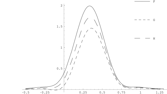
Figure 43: Single-quark contributions to the distribution functions in the MIT bag model of [14].

The quantities $F(x)$, $G(x)$ and $H(x)$ are plotted in Fig. 43. As one can see, the transversity distributions are not so different from those for helicity. Since translational invariance is lost, the distributions do not have the correct support. Thus, the integral of $F(x)$ over $x$ between 0 and 1 is not unity, as it should be. In particular, one has $\int_{0}^{1}F(x)\,\d{x}=0.90$. This normalisation problem can be overcome (although in a very ad hoc manner) by integrating between $-\infty$ and $\infty$, since $\int_{-\infty}^{\infty}F(x)\,\d{x}=1$. Proceeding in this manner, for the tensor charges one obtains

$$\delta{u}\equiv\frac{4}{3}\int_{-\infty}^{\infty}H(x)\,\d{x}=1.09\,,\qquad\delta{d}\equiv-\frac{1}{3}\int_{-\infty}^{\infty}H(x)\,\d{x}=-0.27\,,$$ (8.1.22)

to be compared with the axial charges obtained similarly: $\Delta{u}=0.87$ and $\Delta{d}=-0.22$.

Stratmann [211] recomputed $q(x)$, $\Delta{q}(x)$ and $\Delta_{T}{q}(x)$ in the MIT bag model, introducing a Peierls–Yoccoz projection to partially restore the translational invariance. However, he did not perform a VAP calculation. Since the masses of the intermediate states were not computed within the model, the number sum rules turned out to be violated. Another problem of the approach of [211] is that the antiquark distribution functions were evaluated using eqs. (8.1.14a–LABEL:subneg3) (we have already commented on the inconsistency of such a procedure in Sec. 8.1.2).

The MIT bag model was also used to compute the transversity distributions in [212]. The technique adopted in this work is rather different from that discussed above and is based on a non-relativistic reduction of the relativistic wave function (for a discussion of this non-covariant approach see also [213]). The results of [212] for $h_{1}={\textstyle\frac{1}{2}}\sum_{f}e_{f}^{2}\Delta_{T}{q}_{f}$ and $g_{1}={\textstyle\frac{1}{2}}\sum_{f}e_{f}^{2}\Delta{q}_{f}$ are shown in Fig. 44.

Figure 44: The transversity distribution $h_{1}(x,Q_{0}^{2})$ (continuous line) and the spin distribution function $g_{1}(x,Q_{0}^{2})$ (dashed line) for the MIT bag model at the initial scale $Q_{0}^{2}$. The corresponding evolved distributions $h_{1}(x,Q^{2})$ (dotted line) and $g_{1}(x,Q^{2})$ (dot–dashed line) are obtained starting from (a) $Q_{0}^{2}=0.079\,\text{GeV}^{2}$ and (b) $Q_{0}^{2}=0.75\,\text{GeV}^{2}$. From [212].

8.1.4 Transversity distributions in the CDM

The transversity distributions were calculated in the colour dielectric model in [98]. In particular, the chiral version of the CDM was used, in which the splitting between the masses of the nucleon and delta resonance, or between the scalar and vector diquark, is due to the exchange of pions, instead of perturbative gluons. Although this model suffers a number of drawbacks, its main technical advantage with respect to the MIT bag model is that it allows a full VAP procedure to be performed, since confinement is implemented by a dynamical field, not by a static bag surface. For the same reason, the valence-number sum rules turn out to be fulfilled (to within a few percent) if the masses of the intermediate states are consistently computed within the model. As we shall see, the Soffer inequalities are also satisfied, for both quarks and antiquarks.

The Lagrangian of the chiral CDM is

$$\mathcal{L} = \text{i}\mathchoice{\makebox[0.0pt][l]{$\displaystyle\kern 2.08334pt\overline{\kern-2.43059pt\phantom{\psi}}$}}{\makebox[0.0pt][l]{$\textstyle\kern 2.08334pt\overline{\kern-2.43059pt\phantom{\psi}}$}}{\makebox[0.0pt][l]{$\scriptstyle\kern 1.45834pt\overline{\kern-1.7014pt\phantom{\psi}}$}}{\makebox[0.0pt][l]{$\scriptscriptstyle\kern 1.04167pt\overline{\kern-1.21529pt\phantom{\psi}}$}}\psi\gamma^{\mu}\partial_{\mu}\psi+\frac{g}{\chi}\,\mathchoice{\makebox[0.0pt][l]{$\displaystyle\kern 2.08334pt\overline{\kern-2.43059pt\phantom{\psi}}$}}{\makebox[0.0pt][l]{$\textstyle\kern 2.08334pt\overline{\kern-2.43059pt\phantom{\psi}}$}}{\makebox[0.0pt][l]{$\scriptstyle\kern 1.45834pt\overline{\kern-1.7014pt\phantom{\psi}}$}}{\makebox[0.0pt][l]{$\scriptscriptstyle\kern 1.04167pt\overline{\kern-1.21529pt\phantom{\psi}}$}}\psi\left(\sigma+\text{i}\gamma_{5}\mathchoice{\mbox{\boldmath$\displaystyle\tau$\unboldmath}}{\mbox{\boldmath$\textstyle\tau$\unboldmath}}{\mbox{\boldmath$\scriptstyle\tau$\unboldmath}}{\mbox{\boldmath$\scriptscriptstyle\tau$\unboldmath}}{\cdot}\mathchoice{\mbox{\boldmath$\displaystyle\pi$\unboldmath}}{\mbox{\boldmath$\textstyle\pi$\unboldmath}}{\mbox{\boldmath$\scriptstyle\pi$\unboldmath}}{\mbox{\boldmath$\scriptscriptstyle\pi$\unboldmath}}\right)\psi$$ (8.1.23)

$$+ {\textstyle\frac{1}{2}}\left(\partial_{\mu}\chi\right)^{2}-{\textstyle\frac{1}{2}}M^{2}\chi^{2}+{\textstyle\frac{1}{2}}\left(\partial_{\mu}\sigma\right)^{2}+{\textstyle\frac{1}{2}}\left(\partial_{\mu}\mathchoice{\mbox{\boldmath$\displaystyle\pi$\unboldmath}}{\mbox{\boldmath$\textstyle\pi$\unboldmath}}{\mbox{\boldmath$\scriptstyle\pi$\unboldmath}}{\mbox{\boldmath$\scriptscriptstyle\pi$\unboldmath}}\right)^{2}-U\left(\sigma,\mathchoice{\mbox{\boldmath$\displaystyle\pi$\unboldmath}}{\mbox{\boldmath$\textstyle\pi$\unboldmath}}{\mbox{\boldmath$\scriptstyle\pi$\unboldmath}}{\mbox{\boldmath$\scriptscriptstyle\pi$\unboldmath}}\right),$$

where $U(\sigma,\mathchoice{\mbox{\boldmath$\displaystyle\pi$\unboldmath}}{\mbox{\boldmath$\textstyle\pi$\unboldmath}}{\mbox{\boldmath$\scriptstyle\pi$\unboldmath}}{\mbox{\boldmath$\scriptscriptstyle\pi$\unboldmath}})$ is the usual Mexican-hat potential, see e.g., [214]. $\mathcal{L}$ describes a system of interacting quarks, pions, sigma and a scalar–isoscalar chiral singlet field $\chi$. The chromodielectric field $\chi$ incorporates non-perturbative gluonic degrees of freedom. Through their interaction with the $\chi$ field, the quarks acquire a mass that increases strongly at the boundary of the bag, hence leading to absolute confinement.

The parameters of the model are: the chiral meson masses $m_{\pi}=0.14\,\text{GeV}$, $m_{\sigma}=1.2\,\text{GeV}$ (the precise value of this parameter is actually irrelevant), the pion decay constant $f_{\pi}=93\,\text{MeV}$, the quark–meson coupling constant $g$, and the mass $M$ of the $\chi$ field. The parameters $g$ and $M$, which are the only free parameters of the model, can be uniquely fixed by reproducing the average nucleon–delta mass and the isoscalar radius of the proton.

The chiral CDM Lagrangian (8.1.23) contains a single-minimum potential for the chromodielectric field $\chi$: $V(\chi)={{\textstyle\frac{1}{2}}}M^{2}\chi^{2}$. A double-minimum version of the CDM is also widely studied and used (see for instance [215]). The structure functions computed in the two versions of the chiral CDM do not differ sensibly.

The solution of the field equations for the chiral CDM proceeds through the introduction of the so-called hedgehog ansatz, which corresponds to a mean-field approximation [217]. The technique used to compute the physical nucleon state is based on a double projection of the mean-field solution onto linear- and angular-momentum eigenstates. This technique has also been used to compute the static properties of the nucleon [214], the unpolarised and the longitudinally polarised distribution functions [215], and the nucleon electromagnetic form factors [218]. We refer the reader to these papers for more detail. A different technique to obtain states of definite angular momentum and isospin, based on the quantisation of the collective degrees of freedom associated with the rotation of the hedgehog state, will be mentioned in Sec. 8.2.1. Let us simply remark that in the chiral CDM the chiral field cannot develop a non-zero winding number and its value is always very small. Thus, the choice of a specific technique to obtain physical states from the hedgehog is less critical in the chiral CDM than in other models.

Figure 45: The transversity distributions $x\Delta_{T}{q}(x)$ in the colour dielectric model (from [98]). Left: the quark distributions $x\Delta_{T}{u}$ and $x\Delta_{T}{d}$. Right: the antiquark distributions $x\Delta_{T}\bar{u}$ and $x\Delta_{T}\bar{d}$. The distributions are shown at the model scale $Q_{0}^{2}=0.16\,\text{GeV}^{2}$ and at $Q^{2}=25\,\text{GeV}^{2}$.

In Fig. 45 we show the results of the calculation in [98]. One of the features of the distributions computed in the CDM is their rapid falloff and vanishing for $x>0.6$. This is due to the soft confinement of quarks, which do not carry large momenta. It should also be stressed that the Peierls–Yoccoz procedure, which is a non-relativistic approximation, becomes unreliable at large $x$. Note also that the sea contribution is rather small.

As for the model scale $Q_{0}^{2}$, in [219, 215, 98] it was determined by matching the value of the momentum fraction carried by the valence, as computed in the model, with that obtained by evolving backward the value experimentally determined at large $Q^{2}$. The result is $Q_{0}^{2}=0.16\,\text{GeV}^{2}$. Proceeding in a similar manner, Stratmann found $Q_{0}^{2}=0.08\,\text{GeV}^{2}$ [211] in the MIT bag. The CDM distributions evolved from $Q_{0}^{2}=0.16\,\text{GeV}^{2}$ to $Q^{2}=25\,\text{GeV}^{2}$ are also shown in Fig. 45. Needless to say, perturbative evolution from such low $Q_{0}^{2}$ values should be taken with some caution. The tensor charges computed in the CDM are (at $Q_{0}^{2}=0.16\,\text{GeV}^{2}$)

$$\delta{u}=1.22\,,\qquad\delta{d}=-0.31\,,$$ (8.1.24)

whereas the axial charges are $\Delta{u}=1.08$ and $\Delta{d}=-0.29$ (see Table 6).

8.2 Chiral models

In chiral models the $q\mathchoice{\makebox[0.0pt][l]{$\displaystyle\kern 1.29167pt\overline{\kern-1.50696pt\phantom{q}}$}}{\makebox[0.0pt][l]{$\textstyle\kern 1.29167pt\overline{\kern-1.50696pt\phantom{q}}$}}{\makebox[0.0pt][l]{$\scriptstyle\kern 0.90417pt\overline{\kern-1.05487pt\phantom{q}}$}}{\makebox[0.0pt][l]{$\scriptscriptstyle\kern 0.64583pt\overline{\kern-0.75348pt\phantom{q}}$}}q$ excitations are described in terms of effective degrees of freedom represented by chiral fields. There is now a huge variety of models of this type and, as already seen in Sec. 8.1, bag-like models also admit chiral versions. In this section we shall focus on two models: the chiral quark soliton model (CQSM) [220, 221], which can be also derived from the Nambu–Jona-Lasinio model by imposing non-linear constraints on the chiral fields[222, 223, 224, 225, 226, 227, 228], and the chiral quark model (CQM) [229].

The main difference between these two models is that in the CQSM chiral symmetry is dynamically broken within the model itself, while in the CQM quarks have large dynamical masses arising from a process of spontaneous chiral-symmetry breaking which is not described by the model. Another important difference, reflected in the naming of the two models, is that in the CQSM a non-trivial topology is introduced, which is crucial for stabilising the soliton, whereas in the CQM chiral fields are treated as a perturbation. Finally, while the CQSM is a non-confining model, confinement may be introduced into the CQM, starting from a non-chiral confining model and dressing the quarks with chiral fields.

As for the nucleon spin structure, chiral models are characterised by a depolarisation of the valence quarks, due to a transfer of total angular momentum of the nucleon into the orbital angular momentum of the sea, described by the chiral fields. This feature has made the chiral models quite popular for the study of the nucleon spin structure.

8.2.1 Chiral quark–soliton model

The basic idea of the chiral quark–soliton model is to describe the low-energy behaviour of QCD by two effective degrees of freedom, Nambu–Goldstone pions and quarks with a dynamical mass. The model is described by the following vacuum functional [220, 221]

$$\exp\left\{\text{i}S_{\text{eff}}[\pi(x)]\right\}=\int D\psi\,D\mathchoice{\makebox[0.0pt][l]{$\displaystyle\kern 2.08334pt\overline{\kern-2.43059pt\phantom{\psi}}$}}{\makebox[0.0pt][l]{$\textstyle\kern 2.08334pt\overline{\kern-2.43059pt\phantom{\psi}}$}}{\makebox[0.0pt][l]{$\scriptstyle\kern 1.45834pt\overline{\kern-1.7014pt\phantom{\psi}}$}}{\makebox[0.0pt][l]{$\scriptscriptstyle\kern 1.04167pt\overline{\kern-1.21529pt\phantom{\psi}}$}}\psi\exp\left\{\text{i}\int\!\d^{4}x\,\mathchoice{\makebox[0.0pt][l]{$\displaystyle\kern 2.08334pt\overline{\kern-2.43059pt\phantom{\psi}}$}}{\makebox[0.0pt][l]{$\textstyle\kern 2.08334pt\overline{\kern-2.43059pt\phantom{\psi}}$}}{\makebox[0.0pt][l]{$\scriptstyle\kern 1.45834pt\overline{\kern-1.7014pt\phantom{\psi}}$}}{\makebox[0.0pt][l]{$\scriptscriptstyle\kern 1.04167pt\overline{\kern-1.21529pt\phantom{\psi}}$}}\psi\,(\text{i}\gamma^{\mu}\partial_{\mu}-mU^{\gamma_{5}})\,\psi\right\},$$ (8.2.1)

with

$$U = \exp\left[\text{i}\pi^{a}(x)\tau^{a}\right],$$ (8.2.2a)

$$U^{\gamma_{5}} = \exp\left[\text{i}\pi^{a}(x)\tau^{a}\gamma_{5}\right]={\textstyle\frac{1}{2}}(1+\gamma_{5})\,U+{\textstyle\frac{1}{2}}(1-\gamma_{5})\,U^{\dagger}\,.$$ (8.2.2b)

Here $\psi$ is the quark field, $m$ is the effective quark mass arising from the spontaneous breakdown of chiral symmetry, and $U$ is the SU(2) chiral pion field. A possible derivation of the effective action (8.2.1) is based on the instanton model of QCD vacuum [220].

The CQSM describes the nucleon as a state of $N_{\text{c}}$ valence quarks bound by a self-consistent hedgehog-like pion field whose energy, in fact, coincides with the aggregate energy of quarks from the negative-energy Dirac continuum. This model differs from the $\sigma$-model [201, 202] in that no kinetic energy is associated to the chiral fields, which are effective degrees of freedom, totally equivalent to the $q\mathchoice{\makebox[0.0pt][l]{$\displaystyle\kern 1.29167pt\overline{\kern-1.50696pt\phantom{q}}$}}{\makebox[0.0pt][l]{$\textstyle\kern 1.29167pt\overline{\kern-1.50696pt\phantom{q}}$}}{\makebox[0.0pt][l]{$\scriptstyle\kern 0.90417pt\overline{\kern-1.05487pt\phantom{q}}$}}{\makebox[0.0pt][l]{$\scriptscriptstyle\kern 0.64583pt\overline{\kern-0.75348pt\phantom{q}}$}}q$ excitations of the Dirac sea (the problem of double counting does not arise).

The CQSM field equations are solved as follows. For a given time-independent pion field $U=\exp(\text{i}\pi^{a}(\mathchoice{\mbox{\boldmath$\displaystyle x$\unboldmath}}{\mbox{\boldmath$\textstyle x$\unboldmath}}{\mbox{\boldmath$\scriptstyle x$\unboldmath}}{\mbox{\boldmath$\scriptscriptstyle x$\unboldmath}})\tau^{a})$, one finds the spectrum of the Dirac Hamiltonian:

$$H\Phi_{n}=E_{n}\Phi_{n}\,,$$ (8.2.3)

which contains the upper and lower Dirac continua (distorted by the presence of the external pion field), and may also contain discrete bound-state levels, if the pion field is strong enough. If the pion field has winding number 1, there is exactly one bound-state level which travels all the way from the upper to the lower Dirac continuum as one increases the spatial size of the pion field from zero to infinity. This level must be filled to obtain a non-zero baryon-number state. Since the pion field is colour blind, in the discrete level one may place $N_{\text{c}}$ quarks in a state that is antisymmetric in colour.

Calling $E_{\text{lev}}$ (with $-M\leq{E}_{\text{lev}}\leq{M}$) the energy of the discrete level, the nucleon mass is obtained by adding ${N_{\text{c}}}E_{\text{lev}}$ to the energy of the pion field (which coincides exactly with the overall energy of the lower Dirac continuum) and subtracting the free continuum. The self-consistent pion field is thus found by minimising the functional

$$M=\min_{U}N_{\text{c}}\left\{E_{\text{lev}}[U]+\sum_{E_{n}<0}\left(E_{n}[U]-E_{n}^{(0)}\right)\right\}.$$ (8.2.4)

From symmetry considerations one looks for the minimum in a hedgehog configuration

$$U_{c}({\bf x})=\exp\left[\text{i}\pi^{a}(\mathchoice{\mbox{\boldmath$\displaystyle x$\unboldmath}}{\mbox{\boldmath$\textstyle x$\unboldmath}}{\mbox{\boldmath$\scriptstyle x$\unboldmath}}{\mbox{\boldmath$\scriptscriptstyle x$\unboldmath}})\tau^{a}\right]=\exp\left[\text{i}(\mathchoice{\mbox{\boldmath$\displaystyle n$\unboldmath}}{\mbox{\boldmath$\textstyle n$\unboldmath}}{\mbox{\boldmath$\scriptstyle n$\unboldmath}}{\mbox{\boldmath$\scriptscriptstyle n$\unboldmath}}{\cdot}\mathchoice{\mbox{\boldmath$\displaystyle\tau$\unboldmath}}{\mbox{\boldmath$\textstyle\tau$\unboldmath}}{\mbox{\boldmath$\scriptstyle\tau$\unboldmath}}{\mbox{\boldmath$\scriptscriptstyle\tau$\unboldmath}})P(r)\right],\quad r=|{\mathchoice{\mbox{\boldmath$\displaystyle x$\unboldmath}}{\mbox{\boldmath$\textstyle x$\unboldmath}}{\mbox{\boldmath$\scriptstyle x$\unboldmath}}{\mbox{\boldmath$\scriptscriptstyle x$\unboldmath}}}|\,,\quad\mathchoice{\mbox{\boldmath$\displaystyle n$\unboldmath}}{\mbox{\boldmath$\textstyle n$\unboldmath}}{\mbox{\boldmath$\scriptstyle n$\unboldmath}}{\mbox{\boldmath$\scriptscriptstyle n$\unboldmath}}=\frac{\mathchoice{\mbox{\boldmath$\displaystyle x$\unboldmath}}{\mbox{\boldmath$\textstyle x$\unboldmath}}{\mbox{\boldmath$\scriptstyle x$\unboldmath}}{\mbox{\boldmath$\scriptscriptstyle x$\unboldmath}}}{r}\,,$$ (8.2.5)

where $P(r)$ is the profile of the soliton. The latter is then obtained using a variational procedure.

At lowest order in $1/N_{\text{c}}$, the CQSM essentially corresponds to a mean-field picture. Some observables, however, vanish at zeroth order in $1/N_{\text{c}}$ (this is the case, as we shall see, of unpolarised isovector and polarised isoscalar distribution functions) and for these quantities a calculation at first order in $1/N_{\text{c}}$ is clearly needed.

Within the CQSM several calculations of distribution functions have been performed [230, 231, 232, 233, 234]. In particular, the transversity distributions were computed in [235, 236, 237, 238]. The calculations mainly differ in the order of $1/N_{\text{c}}$ expansion considered. We shall see that this expansion is related to the expansion in the collective angular velocity $\Omega$ of the hedgehog solution, and hence to the collective quantisation of the hedgehog solitons.

Figure 46: Longitudinal and transverse polarisation distributions in the valence-quark approximation of [237].

The first application of the CQSM to transversity is contained in [235], where only the tensor charges were computed. In that paper the CQSM was extended from two to three flavours with a chiral $\text{SU}(3)_{R}\bigotimes\text{SU}(3)_{L}$ symmetry (for a review see [239]). Corrections of order $1/N_{\text{c}}$ were taken into account in building the quantised soliton. The procedure adopted in [235] for constructing states with definite spin and flavour out of the hedgehog is the so-called cranking procedure [203, 240]. The parameters of the model are the constituent mass of the $u$ and $d$ quarks, the explicit SU(3) symmetry breaking term for the mass of the $s$ quark, and a cutoff needed to render the theory finite. These parameters are fixed from hadronic spectroscopy. In particular the constituent mass of the quarks is $m=420\,\text{MeV}$ and the symmetry breaking term corresponds to an extra mass of $180\,\text{MeV}$ for the $s$ quark. The values of the tensor charges obtained are (the model scale is taken to be $Q_{0}^{2}=0.36\,\text{GeV}^{2}$, see Table 6)

$$\delta{u}=1.12\,,\qquad\delta{d}=-0.42\,,\qquad\delta{s}=-0.01\,.$$ (8.2.6)

These quantities are not much affected by the value of the constituent mass and of the SU(3) symmetry breaking term.

We stress the importance of the $1/N_{\text{c}}$ corrections. Without these corrections the tensor (and also the axial) charge of the $u$ quark would be equal and opposite to that of the $d$ quark. It is also important to notice that, while the axial singlet charge is substantially reduced owing to the presence of the chiral fields, the tensor charges are close to those obtained in other models where the chiral fields are absent, or play a minor rôle.

A first attempt to compute the $x$ dependence of the transversity distributions in the CQSM was made in [236]. In this calculation, however, no $1/N_{\text{c}}$ corrections were taken into account, and hence they obtained $\Delta_{T}{u}+\Delta_{T}{d}=0$, which is a spurious – and unrealistic – consequence of the zeroth-order approximation adopted. The two most sophisticated calculations in the CQSM are those of [237] and [238]. In [237], both centre-of-mass motion corrections and $1/N_{\text{c}}$ contributions were taken into account. The correct support for the distributions is obtained by using a procedure that transforms the distributions computed in the rest frame into the distributions in the infinite momentum frame. This procedure essentially amounts to using the relation

$$f_{\text{IMF}}(x)=\frac{\Theta(1-x)}{1-x}f_{\text{RF}}(-\ln(1-x))\,.$$ (8.2.7)

An important limitation of this work is that only the valence contribution to the distribution functions is considered. The transversity distributions at the scale of the model as computed in [237] are shown in Fig. 46.

Wakamatsu and Kubota [238] went beyond the valence-quark approximation of [237] and included vacuum-polarisation effects. Thus they were also able to compute the antiquark distributions, which had only been previously evaluated in [98]. A further improvement is the treatment of the temporal non-locality of the bilinear operators which appear in the distribution functions. The generic operator $A^{\dagger}(0)O_{a}A(\xi^{-})$ is expanded as (see [241])

$$A^{\dagger}(0)O_{a}A(\xi^{-})\simeq\widetilde{O}_{a}+\text{i}\,\xi^{-}\,{\textstyle\frac{1}{2}}\left\{\Omega,\widetilde{O}_{a}\right\},$$ (8.2.8)

where $\widetilde{O}_{a}\equiv{A}^{\dagger}(0)O_{a}A(0)$ and $\Omega=-\text{i}\,A^{\dagger}(t)\,\dot{A}(t)$. Equation (8.2.8) implies that the non-locality of the operator $A^{\dagger}(0)O_{a}A(\xi^{-})$ causes a rotational correction proportional to the collective angular velocity $\Omega$.

Figure 47: Longitudinal and transverse polarisation distributions of quarks, at the scale of the model and after the perturbative evolution. From [238].

In contrast to the calculation of [237], in [238] no centre-of-mass motion corrections are performed and therefore the distributions do not have the correct support. The antiquark distributions are obtained using the relations (8.1.14a–LABEL:subneg3), and the caveat concerning such a procedure thus applies. In Figs. (47,48) the quark and antiquark helicity and transversity distributions computed in [238] are shown. While the quark distributions are not too different from those computed in the CDM (see Fig. 45), the $\delta_{T}\mathchoice{\makebox[0.0pt][l]{$\displaystyle\kern 1.29167pt\overline{\kern-1.50696pt\phantom{u}}$}}{\makebox[0.0pt][l]{$\textstyle\kern 1.29167pt\overline{\kern-1.50696pt\phantom{u}}$}}{\makebox[0.0pt][l]{$\scriptstyle\kern 0.90417pt\overline{\kern-1.05487pt\phantom{u}}$}}{\makebox[0.0pt][l]{$\scriptscriptstyle\kern 0.64583pt\overline{\kern-0.75348pt\phantom{u}}$}}u$ distribution has a different sign. This is a consequence of the different technique used in the calculation of antiquark distributions in [98] and [238] (explicit evaluation of $\Delta_{T}\mathchoice{\makebox[0.0pt][l]{$\displaystyle\kern 1.29167pt\overline{\kern-1.50696pt\phantom{q}}$}}{\makebox[0.0pt][l]{$\textstyle\kern 1.29167pt\overline{\kern-1.50696pt\phantom{q}}$}}{\makebox[0.0pt][l]{$\scriptstyle\kern 0.90417pt\overline{\kern-1.05487pt\phantom{q}}$}}{\makebox[0.0pt][l]{$\scriptscriptstyle\kern 0.64583pt\overline{\kern-0.75348pt\phantom{q}}$}}q$ in [98] vs. use of (8.1.14a–LABEL:subneg3) in [238]). The tensor charges obtained in [238] are (again at $Q_{0}^{2}=0.36\,\text{GeV}^{2}$, see Table 6)

$$\delta{u}=0.89\,,\qquad\delta{d}=-0.33\,.$$ (8.2.9)

Very recently the technique adopted in [238] was criticised in [242]. In this work, however, the isoscalar and isovector distributions are computed at a different order in $1/N_{\text{c}}$ and cannot therefore be combined to give the single-flavour distributions.

Figure 48: Longitudinal and transverse polarisation distributions of antiquarks, at the scale of the model and after the perturbative evolution. From [238].

8.2.2 Chiral quark model

In the chiral quark model of Manohar and Georgi [229] the relevant degrees of freedom at a scale below $1\,\text{GeV}$ are constituent quarks and Goldstone bosons. This model was used in [243] to compute the quark and antiquark distribution functions. The CQM is particularly interesting for the study of the nucleon spin structure, as it predicts a depolarisation of constituent quarks due to the emission of Goldstone bosons into $P$-wave states.

In the CQM model, the $u$, $d$ and $s$ quarks are assumed to develop large dynamical masses as a consequence of a mechanism of spontaneous chiral-symmetry breaking, which lies outside the model itself. We denote these “bare” massive states by $\left|u_{0}\right\rangle$, $\left|d_{0}\right\rangle$ etc. Once they are dressed by Goldstone bosons, the constituent $u$ and $d$ quark states are

$$|u\rangle = \sqrt{Z}\,|u_{0}\rangle+a_{\pi}\,|d\,\pi^{+}\rangle+\frac{a_{\pi}}{2}\,|u\,\pi^{0}\rangle+a_{K}\,|s\,K^{+}\rangle+\frac{a_{\eta}}{6}\,|u\,\eta\rangle\,,\qquad$$ (8.2.10a)

$$|d\rangle = \sqrt{Z}\,|d_{0}\rangle+a_{\pi}\,|u\,\pi^{-}\rangle+\frac{a_{\pi}}{2}\,|d\,\pi^{0}\rangle+a_{K}\,|s\,K^{0}\rangle+\frac{a_{\eta}}{6}\,|d\,\eta\rangle\,,\qquad$$ (8.2.10b)

where $Z$ is the renormalisation constant for a “bare” constituent quark (it turns out to be about $0.7$) and $|a_{i}|^{2}$ are the probabilities of finding the Goldstone bosons in the dressed constituent quark states. These probabilities are related to each other by the underlying $\text{SU}(3)_{R}\otimes\text{SU}(3)_{L}$ symmetry of the model. There is a single free parameter which may be fixed by computing the axial coupling $g_{A}$. Thus the CQM is a perturbative effective theory in the Goldstone boson expansion.

There are three types of contributions to the quark distribution functions. The first corresponds to the probability of finding a bare quark $f_{0}$ inside a dressed quark $f$, and is the bare quark distribution renormalised by the $Z$ factor. The other two contributions correspond to diagrams (a) and (b) of Fig. 49. The spin-independent term corresponding to diagram (a) is given by

$$q_{j}(x)=\int_{x}^{1}\!\frac{\d{y}}{y}\,P_{j\,\alpha/i}(y)\,q_{i}\left(\frac{x}{y}\right).$$ (8.2.11)

Here the splitting function $P(y)_{j\,\alpha/i}$ is the probability of finding a constituent quark $j$ carrying a momentum fraction $y$ and a (spectator) Goldstone boson $\alpha$ ($\alpha=\pi,K,\eta$) inside a constituent quark $i$. Diagram (b) of Fig. 49 corresponds to probing the internal structure of the Goldstone bosons. This process gives the following contribution

$$q_{k}(x)=\int\!\frac{\d{y}_{1}}{y_{1}}\,\frac{\d{y}_{2}}{y_{2}}\,V_{k/\alpha}\left(\frac{x}{y_{1}}\right)P_{\alpha\,j/i}\left(\frac{y_{1}}{y_{2}}\right)q_{i}(y_{2})\,,$$ (8.2.12)

where $V_{k/\alpha}(x)$ is the distribution function of quarks of flavour $k$ inside the Goldstone boson $\alpha$. In analogy with (8.2.11, 8.2.12), the longitudinal and transverse polarisation distributions contain the splitting functions $\Delta{P}(y)$ and $\Delta_{T}{P}(y)$, respectively.

Figure 49: Diagrams contributing to the constituent quark structure: (a) the Goldstone boson spectator process, (b) the process probing the structure of the Goldstone boson. The solid lines represent quarks and dashed lines represent Goldstone bosons. From [243].

In [243] the splitting functions are computed within the CQM, the bare quark distributions are obtained from a covariant quark–diquark model [244, 18, 245], and the quark distribution functions in the Goldstone bosons are taken from phenomenological parametrisations [193] for pions and from models [246, 247, 248] for kaons. The following relation is found

$$P(y)+\Delta{P}(y)=2\Delta_{T}{P}(y)\,,$$ (8.2.13)

which implies saturation of the Soffer inequality.

The dominant contribution to the dressing of the constituent quarks is due to pion emission. The pion cloud affects the $u$ sector reducing both the helicity and transversity distributions in a similar manner, as can be seen in Fig. 50. The situation is quite different in the $d$ sector. In fact, while the renormalisation and meson cloud corrections approximately cancel each other in the helicity distribution $\Delta{d}$, for the transversity distribution $\Delta_{T}{d}$ these corrections are both positive. Thus, with respect to the bare distributions, $\Delta{d}$ is almost unmodified whereas $\Delta_{T}{d}$ is drastically reduced. The difference between $\Delta{d}(x)$ and $\Delta_{T}{d}(x)$ is an important and peculiar feature of the model of [243]; the results for the $d$ distributions are shown in Fig. 51. One can see that the meson cloud suppresses $\Delta_{T}{d}$ much more than its helicity counterpart. In terms of tensor charges, $\delta{d}$ is reduced by about 40% by the pion depolarisation effect while the corresponding axial charge is almost unchanged. The tensor and axial charges are collected in Table 6. Notice that depolarisation due to Goldstone boson emission is a significant effect, although not sufficient to reproduce the small value of $\Delta\Sigma$ observed experimentally.

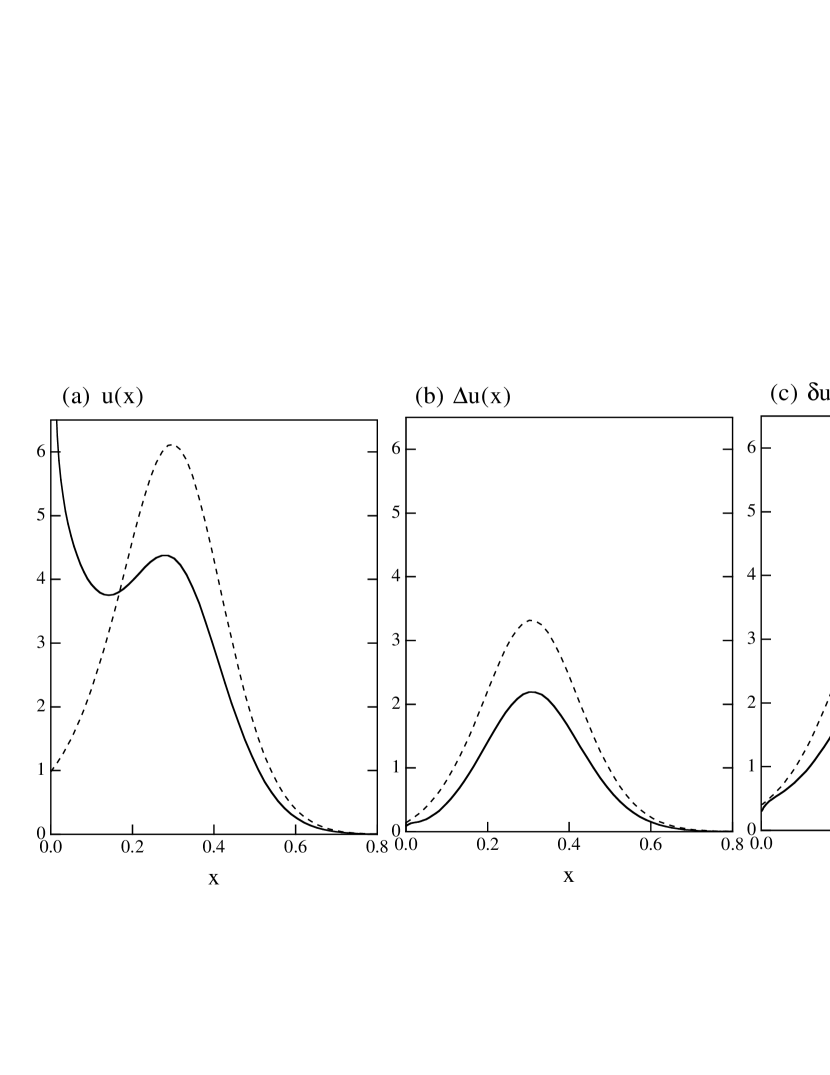
Figure 50: The $u$-quark distribution functions: (a) $u(x)$, (b) $\Delta{u}(x)$ and (c) $\Delta_{T}{u}(x)$, respectively. In each figure, the result with dressed constituent quarks is shown by the solid curve and that without dressing by the dashed curve. The latter corresponds to the spectator model calculation of [245] (see Sec. 8.4). From [243].

8.3 Light-cone models

This section is devoted to models using the so-called front-form dynamics to describe the nucleon in the infinite momentum frame, and the Melosh rotation to transform rest-frame quark states into infinite momentum states.

We start by recalling the general idea of front-form dynamics, originally due to Dirac [249], and then present the calculations of the transversity distributions based on this approach.

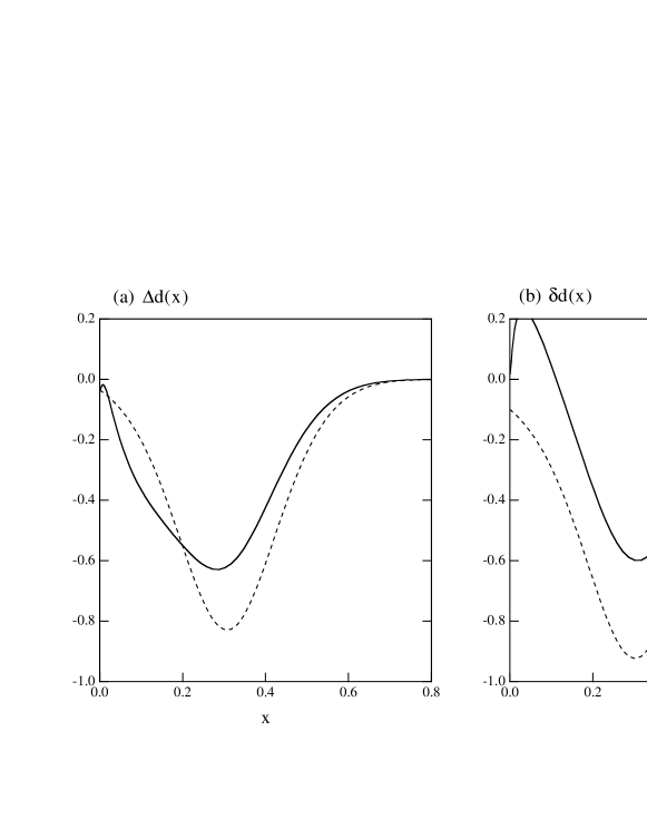
Figure 51: The $d$-quark distribution functions: (a) $\Delta{d}(x)$ and (b) $\Delta_{T}{d}(x)$, respectively. The notation is the same as in Fig. 50. From [243].

8.3.1 Forms of dynamics and Melosh rotation

As shown by Dirac [249] (see also [250]), we have in general a certain freedom in describing the dynamics of a system. Various choices of variables defining the initial conditions and of operators generating the evolution of the system are possible. We shall refer to each of these choices as a “form” of dynamics.

The state of a system is defined on a hypersurface $\Sigma$ in Minkowski space that does not contain time-like directions. To characterise the state unambiguously, $\Sigma$ must intersect every world-line once and only once. The most familiar example of such a surface is, of course, the time instant $x^{0}=0$.

Among the ten generators of the Poincaré algebra, there are some that map $\Sigma$ into itself, not affecting the time evolution, and others that drive the evolution of the system and contain the entire dynamics. The latter generators are called Dirac “Hamiltonians”.

Hereafter we shall only be interested in two forms of dynamics: the instant-form and the front-form (for a more general discussion we refer the reader to [250]).

In the usual form of dynamics, the instant-form, the initial conditions are set at some instant of time and the hypersurfaces $\Sigma$ are flat three-dimensional surfaces only containing directions that lie outside the light-cone. The generators of rotations and space translations leave the instant invariant and do not affect the dynamics. The remaining four generators (boosts and time translations) are the “Hamiltonians”.

In the front-form dynamics one considers instead three-dimensional surfaces in space–time formed by a plane-wave front advancing at the velocity of light, e.g., the surface $x^{+}=0$. The quantities $P^{1}$, $P^{2}$, $P^{+}$, $M^{12}$, $M^{-+}$, $M^{1+}$ and $M^{2+}$ are associated with transformations that leave this front invariant. The remaining Poincaré generators, namely $P^{-}$, $M^{1-}$ and $M^{2-}$ are the “Hamiltonians”. The advantage of using front-form dynamics is that the number of Poincaré generators affecting the dynamics of the system is reduced and there is one more Poincaré generator that transforms the states without evolving them.

Working within front-form dynamics, there is an important transformation, namely the Melosh-Wigner (MW) rotation [251, 252], which relates the spin wave functions $q_{\text{RF}}^{\uparrow\downarrow}$ in the rest frame (RF) to the spin wave functions $q_{\text{IMF}}^{\uparrow\downarrow}$ in the infinite momentum frame (IMF). The Melosh–Wigner rotation is

$$q_{\text{IMF}}^{\uparrow} = w\left[(k^{+}+m)\,q_{\text{RF}}^{\uparrow}+(k^{1}+\text{i}k^{2})\,q_{\text{RF}}^{\downarrow}\right],$$ (8.3.1a)

$$q_{\text{IMF}}^{\downarrow} = w\left[-(k^{1}-\text{i}k^{2})\,q_{\text{RF}}^{\uparrow}+(k^{+}+m)\,q_{\text{RF}}^{\downarrow}\right],$$ (8.3.1b)

where $w=[(k^{+}+m)^{2}+\mathchoice{\mbox{\boldmath$\displaystyle k$\unboldmath}}{\mbox{\boldmath$\textstyle k$\unboldmath}}{\mbox{\boldmath$\scriptstyle k$\unboldmath}}{\mbox{\boldmath$\scriptscriptstyle k$\unboldmath}}_{\perp}^{2}]^{-1/2}$ and $k^{+}=k^{0}+k^{3}$.

The reason that the MW rotation is relevant in DIS is that this process probes quark dynamics on the light-cone rather than the constituent quarks in the rest frame [253, 254]. As for the spin structure, in front-form dynamics the spin of the proton is not simply the sum of the spins of the individual quarks, but is the sum of the MW-rotated spins of the light-cone quarks [255].

Calculations of distribution functions using MW have recently appeared in the literature, see e.g., [256, 257].

8.3.2 Transversity distributions in light-cone models

B.-Q. Ma has reconsidered the problem of the spin of the nucleon in the light of the effects of the MW rotation [258]. Applying the MW rotation, the quark contribution to the spin of the nucleon is reduced. In particular, from eqs.(8.3.1a, LABEL:submelosh2) one can show that the observed (i.e., IMF) axial charge $\Delta{q}_{\text{IMF}}$ is related to the constituent quark axial charge $\Delta{q}_{\text{RF}}$ as follows

$$\Delta{q}_{\text{IMF}}=\langle M_{q}\rangle\,\Delta{q}_{\text{RF}}\,,$$ (8.3.2)

where

$$M_{q}=\frac{(k^{+}+m)^{2}-\mathchoice{\mbox{\boldmath$\displaystyle k$\unboldmath}}{\mbox{\boldmath$\textstyle k$\unboldmath}}{\mbox{\boldmath$\scriptstyle k$\unboldmath}}{\mbox{\boldmath$\scriptscriptstyle k$\unboldmath}}_{\perp}^{2}}{(k^{+}+m)^{2}+\mathchoice{\mbox{\boldmath$\displaystyle k$\unboldmath}}{\mbox{\boldmath$\textstyle k$\unboldmath}}{\mbox{\boldmath$\scriptstyle k$\unboldmath}}{\mbox{\boldmath$\scriptscriptstyle k$\unboldmath}}_{\perp}^{2}}\,,$$ (8.3.3)

and $\langle{M_{q}}\rangle$ is its expectation value in the three-quark state

$$\langle M_{q}\rangle=\int\!\d^{3}\mathchoice{\mbox{\boldmath$\displaystyle k$\unboldmath}}{\mbox{\boldmath$\textstyle k$\unboldmath}}{\mbox{\boldmath$\scriptstyle k$\unboldmath}}{\mbox{\boldmath$\scriptscriptstyle k$\unboldmath}}\,M_{q}\ |\Psi(\mathchoice{\mbox{\boldmath$\displaystyle k$\unboldmath}}{\mbox{\boldmath$\textstyle k$\unboldmath}}{\mbox{\boldmath$\scriptstyle k$\unboldmath}}{\mbox{\boldmath$\scriptscriptstyle k$\unboldmath}})|^{2}\,,$$ (8.3.4)

where $\Psi(\mathchoice{\mbox{\boldmath$\displaystyle k$\unboldmath}}{\mbox{\boldmath$\textstyle k$\unboldmath}}{\mbox{\boldmath$\scriptstyle k$\unboldmath}}{\mbox{\boldmath$\scriptscriptstyle k$\unboldmath}})$ is the (normalised) momentum wavefunction of the three-quark state. By choosing two different reasonable wave functions (harmonic oscillator and power-law fall off) the calculation in [259] gives $\langle{M_{q}}\rangle=0.75$ (both for $u$ and $d$ if we assume $m_{u}=m_{d}$), which leads to a reduction of $\Delta\Sigma$ from $1$ (the constituent quark model value) down to $0.75$.

The effect of the MW rotation on the tensor charges was discussed in [92]. One finds that the IMF tensor charge is related to the constituent quark tensor charge by

$$\delta{q}_{\text{IMF}}=\langle\widetilde{M}_{q}\rangle\,\delta{q}_{\text{RF}}\,,$$ (8.3.5)

where

$$\widetilde{M}_{q}=\frac{(k^{+}+m)^{2}}{(k^{+}+m)^{2}+\mathchoice{\mbox{\boldmath$\displaystyle k$\unboldmath}}{\mbox{\boldmath$\textstyle k$\unboldmath}}{\mbox{\boldmath$\scriptstyle k$\unboldmath}}{\mbox{\boldmath$\scriptscriptstyle k$\unboldmath}}_{\perp}^{2}}\,,$$ (8.3.6)

and, again, $\langle\widetilde{M}_{q}\rangle$ is the expectation value of $\widetilde{M}_{q}$. From (8.3.3) and (8.3.6) one finds an important connection between the MW rotation for the longitudinal and the transverse polarisation, namely

$$1+M_{q}=2\widetilde{M}_{q}.$$ (8.3.7)

With the value $\langle{M_{q}}\rangle=0.75$, this implies $\langle\widetilde{M}_{q}\rangle=0.88$ and, using the SU(6) values $\delta_{\text{RF}}=\frac{4}{3}$ and $\delta{d}_{\text{RF}}=-\frac{1}{3}$, one obtains [92] (we omit the “IMF” subscript)

$$\delta{u}=1.17\,,\qquad\delta{d}=-0.29\,.$$ (8.3.8)

The transverse polarisation distributions were computed using the MW rotation in [260]. In this paper a simple relation connecting the spin distributions of quarks in the rest frame $\Delta{q}_{\text{RF}}(x)$, the quark helicity distributions $\Delta{q}(x)$ and the quark transversity distributions $\Delta_{T}{q}(x)$ was derived. It reads

$$\Delta{q}_{\text{RF}}(x)+\Delta{q}(x)=2\Delta_{T}{q}(x)\,.$$ (8.3.9)

Adopting a diquark spectator model [261] to compute the rest-frame distributions, the authors of [260] obtain the curves shown in Fig. 52.

Figure 52: The quark spin distributions $x\Delta{q}_{\text{RF}}(x)$ (solid curves), $x\Delta_{T}{q}(x)$ (dashed curves), and $x\Delta{q}(x)$ (dotted curves) in the light-cone SU(6) quark-spectator model, for (a) $u$ quarks and (b) $d$ quarks. From [260].

From (8.3.9) and the measured values of the quantities $\Gamma^{p,n}\equiv\int\d{x}\,g_{1}^{p,n}$, $g_{A}/g_{V}$ and $\Delta{s}$, it is possible to obtain predictions for the tensor charges, as shown by Ma and Schmidt [262]. Taking $g_{A}/g_{V}=6\,(\Gamma^{p}-\Gamma^{n})$ these authors find (the ranges are determined by the experimental and theoretical uncertainties)

$$\delta{u}=0.84-1.09\,,\qquad\delta{d}=-(0.23-0.51)\,.$$ (8.3.10)

Using the value $g_{A}/g_{V}=1.2573$ from neutron $\beta$ decay (denoted case 2), they find instead

$$\delta{u}=0.89-1.11\,,\qquad\delta{d}=-(0.29-0.53)\,.$$ (8.3.10^′)

Another calculation of the transversity distributions based on the MW rotation is presented in [263]. These authors use a three-quark wave function obtained by solving the Schrödinger equation with a hypercentral phenomenological potential (for details see [256]). The effect of the MW rotation is to introduce a significant difference between longitudinal and transverse polarisation already at the model scale.

8.4 Spectator models

As we have seen, the main ingredients in model calculations of quark distributions are the nucleon–quark vertices and the masses of the intermediate states. In the spectator model the set of intermediate states is reduced to only the diquark states and the vertex is parametrised in some manner, for instance assuming an SU(6) spin–flavour structure. This model was used in [244] to estimate unpolarised and longitudinally polarised distributions and, in [264, 245] to compute the transversity distributions. In [245, 243] it was used as the starting point for the perturbative dressing of quarks by chiral fields.

As already mentioned, the model contains the diquark masses as free parameters. Typical values of these masses are in the range 600–800 MeV, with a splitting of the scalar and vector diquark masses of the order of 100–200 MeV. The parameters entering the vertices are their Dirac structure and form factors. The calculations in [264] and in [245] differ mainly in the choice of the parameters and in a more-or-less simple form for the vertex.

The results of [245] for the distribution functions are those already presented in Sec. 8.2.2 in Figs. 50 and 51 (they correspond to the undressed contributions, i.e., to the dashed curves). Similar results were obtained in [264], where, fixing the parameters so as to obtain the experimental value of the axial coupling, the tensor charges were found to be

$$\delta{u}=1.22\,,\qquad\delta{d}=-0.25\,.$$ (8.4.1)

In [244] the scale of this model was estimated to be $Q_{0}^{2}=0.063\,\text{GeV}^{2}$.

8.5 Non-perturbative QCD calculations

8.5.1 QCD sum rules

In the QCD sum-rule approach (see for instance [265]) one considers correlation functions of the form

$$\Pi(q^{2})=\text{i}\int\!\d^{4}\xi\,\e^{\text{i}q{\cdot}\xi}\,\langle 0|T\left(j(\xi)j(0)\right)|0\rangle\,,$$ (8.5.1)

where $j(x)=\mathchoice{\makebox[0.0pt][l]{$\displaystyle\kern 1.29167pt\overline{\kern-1.50696pt\phantom{q}}$}}{\makebox[0.0pt][l]{$\textstyle\kern 1.29167pt\overline{\kern-1.50696pt\phantom{q}}$}}{\makebox[0.0pt][l]{$\scriptstyle\kern 0.90417pt\overline{\kern-1.05487pt\phantom{q}}$}}{\makebox[0.0pt][l]{$\scriptscriptstyle\kern 0.64583pt\overline{\kern-0.75348pt\phantom{q}}$}}q(x)\Gamma{q}(x)$ is a quark current (all indices are omitted for simplicity). The vacuum polarisation (8.5.1) is computed in two different ways. On one hand, it is modelled by a dispersion relation, expressing its imaginary part in terms of resonances exchanged in the $s$-channel. On the other hand, in the limit of small light-cone separations, i.e., large $Q^{2}\equiv-q^{2}$, one can make an operator-product expansion (OPE) of $T\,(j(\xi)j(0))$, thus relating $\Pi(q^{2})$ to quark condensates $\langle\mathchoice{\makebox[0.0pt][l]{$\displaystyle\kern 1.29167pt\overline{\kern-1.50696pt\phantom{q}}$}}{\makebox[0.0pt][l]{$\textstyle\kern 1.29167pt\overline{\kern-1.50696pt\phantom{q}}$}}{\makebox[0.0pt][l]{$\scriptstyle\kern 0.90417pt\overline{\kern-1.05487pt\phantom{q}}$}}{\makebox[0.0pt][l]{$\scriptscriptstyle\kern 0.64583pt\overline{\kern-0.75348pt\phantom{q}}$}}qq\rangle$. The two theoretical expressions of $\Pi(q^{2})$ are then equated, after performing a Borel transformation, which allows one to pick up only the lowest-lying resonances in a particular channel. The result is an expression for the matrix elements of certain quark currents in a hadron state, in terms of quark and resonance parameters, condensates and the Borel mass $M_{B}$. The generalisation of this procedure to three-point correlators is straight-forward.

A QCD sum rule calculation of the tensor charges was reported by He and Ji in [266]. Following the method presented in [267], they consider the three-point correlation function

$$\Pi^{\mu\nu}(q^{2})=\text{i}^{2}\int\!\d^{4}\xi\,\d^{4}\zeta\,\e^{\text{i}q{\cdot}\xi}\,\langle 0|T\left(j^{\mu\nu}(\zeta)\eta(\xi)\mathchoice{\makebox[0.0pt][l]{$\displaystyle\kern 1.29167pt\overline{\kern-1.50696pt\phantom{\eta}}$}}{\makebox[0.0pt][l]{$\textstyle\kern 1.29167pt\overline{\kern-1.50696pt\phantom{\eta}}$}}{\makebox[0.0pt][l]{$\scriptstyle\kern 0.90417pt\overline{\kern-1.05487pt\phantom{\eta}}$}}{\makebox[0.0pt][l]{$\scriptscriptstyle\kern 0.64583pt\overline{\kern-0.75348pt\phantom{\eta}}$}}\eta(0)\right)|0\rangle\,,$$ (8.5.2)

where $j^{\mu\nu}$ is the quark tensor current

$$j^{\mu\nu}(\zeta)=\mathchoice{\makebox[0.0pt][l]{$\displaystyle\kern 1.29167pt\overline{\kern-1.50696pt\phantom{q}}$}}{\makebox[0.0pt][l]{$\textstyle\kern 1.29167pt\overline{\kern-1.50696pt\phantom{q}}$}}{\makebox[0.0pt][l]{$\scriptstyle\kern 0.90417pt\overline{\kern-1.05487pt\phantom{q}}$}}{\makebox[0.0pt][l]{$\scriptscriptstyle\kern 0.64583pt\overline{\kern-0.75348pt\phantom{q}}$}}q(\zeta)\,\sigma^{\mu\nu}\,q(\zeta)\,,$$ (8.5.3)

and $\eta(\xi)$ is the nucleon interpolating field, i.e.,

$$\eta(\xi)=\varepsilon_{abc}\,[u_{a}^{T}(\xi)C\gamma_{\mu}u_{b}(\xi)]\gamma_{5}\gamma^{\mu}d_{c}(\xi)\,.$$ (8.5.4)

(Here $a$, $b$ and $c$ are colour indices, the superscript $T$ indicates transpose and $C$ is the charge conjugation matrix.) The interpolating current $\eta$ is related to the nucleon spinor $U(P)$ by

$$\langle 0|\eta(0)|P\rangle=\lambda\,U(P)\,,$$ (8.5.5)

where $\lambda$ is a coupling strength.

Computing (8.5.2), using OPE on one hand and resonance saturation on the other, for the tensor charges He and Ji obtained (at a scale $\mu^{2}=M^{2}$)

$$\delta{u}=1.0\pm 0.5\,,\qquad\delta{d}=0.0\pm 0.5\,.$$ (8.5.6)

The uncertainty corresponds to a variation of the Borel mass $M_{B}^{2}$ from $M^{2}$ to $2M^{2}$.

In a subsequent paper [268] He and Ji presented a more refined QCD sum rule calculation of $\delta{q}$ taking into account operators of higher orders. Instead of the three-point function approach adopted in [266], they used the external-field approach. Their starting point is the two-point correlation function in the presence of an external constant tensor field $Z_{\mu\nu}$

$$\Pi^{\mu\nu}(Z_{\mu\nu},q^{2})=\text{i}\int\!\d^{4}\xi\,\e^{\text{i}q{\cdot}\xi}\,\langle 0|T\,(\eta(\xi)\mathchoice{\makebox[0.0pt][l]{$\displaystyle\kern 1.29167pt\overline{\kern-1.50696pt\phantom{\eta}}$}}{\makebox[0.0pt][l]{$\textstyle\kern 1.29167pt\overline{\kern-1.50696pt\phantom{\eta}}$}}{\makebox[0.0pt][l]{$\scriptstyle\kern 0.90417pt\overline{\kern-1.05487pt\phantom{\eta}}$}}{\makebox[0.0pt][l]{$\scriptscriptstyle\kern 0.64583pt\overline{\kern-0.75348pt\phantom{\eta}}$}}\eta(0))|0\rangle_{Z}\,.$$ (8.5.7)

The coupling between quarks and $Z_{\mu\nu}$ is described by the additional term

$$\Delta\mathcal{L}=g_{q}\mathchoice{\makebox[0.0pt][l]{$\displaystyle\kern 1.29167pt\overline{\kern-1.50696pt\phantom{q}}$}}{\makebox[0.0pt][l]{$\textstyle\kern 1.29167pt\overline{\kern-1.50696pt\phantom{q}}$}}{\makebox[0.0pt][l]{$\scriptstyle\kern 0.90417pt\overline{\kern-1.05487pt\phantom{q}}$}}{\makebox[0.0pt][l]{$\scriptscriptstyle\kern 0.64583pt\overline{\kern-0.75348pt\phantom{q}}$}}q\sigma^{\mu\nu}qZ_{\mu\nu}\,,$$ (8.5.8)

in the QCD Lagrangian.

Referring to the original paper for the details of the calculation, we give here the results for $\delta{u}$ and $\delta{d}$ at the scale $\mu^{2}=M^{2}$

$$\delta{u}=1.33\pm 0.53\,,\qquad\delta{d}=0.04\pm 0.02\,,$$ (8.5.9)

where the error is an estimated theoretical one.

A similar study of tensor charges in the QCD sum rule framework was carried out by Jin and Tang [269], who discussed in detail various sources of uncertainty, and in particular the dependence of the results on the vacuum tensor susceptibility induced by the external field.

Finally, we recall that QCD sum rules have been also used to compute the transversity distributions $\Delta_{T}{q}(x)$. This was done in [69] by considering a four-point correlator. The ranges of validity of the various approximations adopted and the sensitivity of the results on the Borel mass considerably restrict the interval of $x$ over which a reliable calculation can be performed. The result of [69] is $\Delta_{T}{u}\simeq 0.5$ for $0.3\lesssim{x}\lesssim 0.5$, with no apparent variation in this range (the $Q^{2}$ scale is estimated to be $Q^{2}\approx 5-10\,\text{GeV}^{2}$).

8.5.2 Lattice

Lattice evaluations of the tensor charges have been presented by various groups [270, 271, 272, 273, 274]. The lattice approach is based on a hypercubic discretisation of the Euclidean path integral for QCD and a Monte Carlo computation of the resulting partition function. The lattice size must be large enough so that finite size effects are small. An important parameter is the lattice spacing $a$. The continuum limit corresponds to $a\to 0$. Usually, different values of quark masses are used and a linear extrapolation is made to the chiral limit of massless quarks.

Aoki et al. [270] performed a simulation on a $16^{3}\times 20$ lattice with spacing $a\simeq 0.14$ fm, in the quenched approximation (which corresponds to setting the fermion determinant in the partition function equal to one). They obtained

$$\delta{u}=0.839(60)\,,\qquad\delta{d}=-0.231(55)\,,$$ (8.5.10)

at a scale $\mu=a^{-1}\simeq 1.4\,\text{GeV}$. For comparison, the axial charges computed with the same lattice configuration are [275]

$$\Delta{u}=0.638(54)\,,\qquad\Delta{d}=-0.347(46)\,.$$ (8.5.11)

Similar results were reported in [272]. The continuum limit was investigated by Capitani et al. [273], who found for the difference $\delta{u}-\delta{d}$ the value

$$\delta{u}-\delta{d}=1.21(4)\,.$$ (8.5.12)

Finally, a lattice calculation of the tensor charges in full QCD (that is, with no quenching assumption) has been recently carried out by Dolgov et al. [274]. Using $16^{3}\times 32$ lattices, these authors obtain

$$\delta{u}=0.963(59)\,,\qquad\delta{d}=-0.202(36)\,.$$ (8.5.13)

8.6 Tensor charges: summary of results

In Table 6 we compare the results for tensor charges computed in the models discussed above. We also show the value of the axial charges.

Table 6: Axial and tensor charges in various models. Tensor charges evolved in LO QCD from the intrinsic scale of the model ($Q_{0}^{2}$) to $Q^{2}=10\,\text{GeV}^{2}$ are also shown. See the text for details.

Model [Ref.]	$\Delta{u}$	$\Delta{d}$	$\Delta\Sigma$	$\delta{u}$	$\delta{d}$	$|\delta{u}/\delta{d}|$	$Q_{0}$[GeV]	$\delta{u}(Q^{2})$	$\delta{d}(Q^{2})$
NRQM $\star$	1.33	-0.33	1	1.33	-0.33	4.03	0.28	0.97	-0.24
MIT [14] $\diamond$	0.87	-0.22	0.65	1.09	-0.27	4.04	0.87	0.99	-0.25
CDM [98] $\oplus$	1.08	-0.29	0.79	1.22	-0.31	3.94	0.40	0.99	-0.25
CQSM1 [235] $\times$	0.90	-0.48	0.37	1.12	-0.42	2.67	0.60	0.97	-0.37
CQSM2 [238] $+$	0.88	-0.53	0.35	0.89	-0.33	2.70	0.60	0.77	-0.29
CQM [243] $\otimes$	0.65	-0.22	0.43	0.80	-0.15	5.33	0.80	0.72	-0.13
LC [92] $\circ$	1.00	-0.25	0.75	1.17	-0.29	4.03	0.28	0.85	-0.21
Spect. [264] $\ast$	1.10	-0.18	0.92	1.22	-0.25	4.88	0.25	0.83	-0.17
Latt. [275, 270] $\triangleright$	0.64	-0.35	0.29	0.84	-0.23	3.65	1.40	0.80	-0.22

To allow a homogeneous comparison, we evolved the tensor charges from the model scales $Q_{0}^{2}$ to $Q^{2}=10\,\text{GeV}^{2}$ in LO QCD. Given the very low input scales, the result of this evolution should be taken with caution (it serves to give a qualitative idea of the trend).

Unfortunately, $Q_{0}$ has not been evaluated in the same manner in all models. As discussed earlier, a possible way to estimate the model scale is to fix it in such a manner that, starting from the computed value of the momentum fraction carried by the valence, and evolving it to larger $Q^{2}$, one fits the experimentally observed value. This procedure, with slight differences, has been adopted to find the intrinsic scale in the non-relativistic quark model (NRQM) [212], in the MIT bag model [186, 211], in the CDM [219, 215, 98] and in the spectator model [244]. For the light-cone (LC) model of [92] we have taken the same scale as in the NRQM, since the starting point of that calculation is the rest-frame spin distributions of quarks. In other calculations, in particular in chiral models, the authors have chosen $Q_{0}$ as the scale up to which the model is expected to incorporate the relevant degrees of freedom. The variety of procedures adopted to determine $Q_{0}$ adds a further element of uncertainty in the results for $\delta{q}(Q^{2})$ presented in Table 6. The evolved tensor charges are collected in Fig. 53. As one can see, they span the ranges

$$\delta{u}=0.7-1\,,\qquad\delta{d}=-(0.1-0.4)\qquad\text{at}\;Q^{2}=10\,\text{GeV}^{2}\,.$$ (8.6.1)

It is important to notice that, since the evolution of the tensor charges is multiplicative, the ratio $\delta{u}/\delta{d}$ does not depend on $Q^{2}$. As one can see from Table 6, most of the calculations give for $|\delta{u}/\delta{d}|$ a value of the order of 4, or larger. Chiral soliton models CQSM1 and CQSM2, in contrast, point to a considerably smaller value, of the order of 2.7. An experimental measurement of the tensor charges may then represent an important test of these models. Note also that the introduction of chiral fields in a perturbative manner, as in the CQM, actually has the effect of increasing $|\delta{u}/\delta{d}|$ owing to a strong reduction in $\delta{d}$. A possible way to extract the $u/d$ transversity ratio is to make a precision measurement of the ratio of azimuthal asymmetries in $\pi^{+}/\pi^{-}$ leptoproduction. This could be done in the not so distant future (see Sec. 10).

Figure 53: The tensor charges as computed in various models and evolved to $Q^{2}=10\,\text{GeV}^{2}$. For the symbols see Table 6. The MIT and CDM points are slightly displaced for clarity.

9 Phenomenology of transversity

We now review some calculations of physical observables (typically, double-spin and single-spin asymmetries) related to transversity. Due to the current lack of knowledge on $\Delta_{T}{q}$ and the related fragmentation functions, the available predictions are quite model-dependent and must be taken with a grain of salt. They essentially provide an indication of the order of magnitude of some phenomenological quantities.

We also discuss two recent results on azimuthal asymmetries in pion leptoproduction that may find an explanation in the coupling of transversity to a $T$-odd fragmentation function arising from final-state interactions.

9.1 Transverse polarisation in hadron–hadron collisions

9.1.1 Transverse double-spin asymmetries in Drell–Yan processes

The Drell–Yan transverse double-spin asymmetries were calculated at LO in [98, 100] and at NLO in [104, 105] (see also [276]). Earlier estimates [21, 277] suffered a serious problem (they assumed the same QCD evolution for $\Delta{q}$ and $\Delta_{T}{q}$), which led to over-optimistic values for $A_{TT}^{\text{DY}}$.

Figure 54: Drell–Yan longitudinal and transverse double-spin asymmetries normalised to the partonic asymmetry, as a function of $x_{a}-x_{b}$ (i.e., $x_{1}-x_{2}$) for two values of the dilepton invariant mass (left), and as a function of the invariant mass of the dilepton pair $M^{2}$ for two values of the c.m. energy (right). From [100].

In [100] the equality $\Delta_{T}{q}(x,Q_{0}^{2})=\Delta{q}(x,Q_{0}^{2})$ was assumed to hold at a very low scale (the input $Q_{0}^{2}=0.23\,\text{GeV}^{2}$ of the GRV distributions [114]), as suggested by various non-perturbative and confinement model calculations (see Sec. 8). The transversity distributions were then evolved according to their own Altarelli–Parisi equation at LO. The resulting asymmetry (divided by the partonic asymmetry) is shown in Fig. 54. Its value is just a few percent, which renders the planned Relativistic Heavy Ion Collider (RHIC) measurement of $A_{TT}^{\text{DY}}$ rather difficult. The asymmetry for the $Z^{0}$-mediated Drell–Yan process is plotted in Fig. 55 and has the same order of magnitude as the electromagnetic one.

Figure 55: Longitudinal and transverse double-spin asymmetries (normalised to the partonic asymmetry) for the $Z^{0}$-mediated Drell–Yan process. From [100].

The authors of [105] use a different procedure to estimate the transversity distributions. They set $|\Delta_{T}{q}|=2\,(q+\Delta{q})$ at the GRV scale, thus imposing the saturation of Soffer’s inequality. This yields the maximal value for $A_{TT}^{\text{DY}}$. The transversity distributions are evolved at NLO. The NLO corrections are found to be relatively small, although non-negligible. The predicted curves for $A_{TT}^{\text{DY}}$ are shown in Fig. 56.

Summarising the results of the calculations of $A_{TT}^{\text{DY}}$, we can say that at the typical energies of the RHIC experiments [278, 279] ($\sqrt{\vphantom{0}}{s}>100\,\text{GeV}$) one expects for the double-spin asymmetry, integrated over the invariant mass $Q^{2}$ of the dileptons, a value

$$A_{TT}^{\text{DY}}\sim(1-2)\%,\quad\text{at most}.$$ (9.1.1)

It is interesting to note that as $\sqrt{\vphantom{0}}{s}$ falls the asymmetry tends to increase, as was first pointed out in [100]. Thus, at $\sqrt{\vphantom{0}}{s}=40\,\text{GeV}$, which would correspond to the c.m. energy of the proposed (but later cancelled) HERA-$\vec{N}$ experiment [280], $A_{TT}^{\text{DY}}$ could reach a value of $\sim(3-4)\%$.

Model calculations of $A_{TT}^{\text{DY}}$ are reported in [98, 263]. The longitudinal–transverse Drell–Yan asymmetry $A_{LT}^{\text{DY}}$ (see Sec. 7.3.1) was estimated in [281, 282] and found to be five to ten times smaller than the double-transverse asymmetry. Polarised proton–deuteron Drell–Yan processes were investigated in [283, 284, 285, 286].

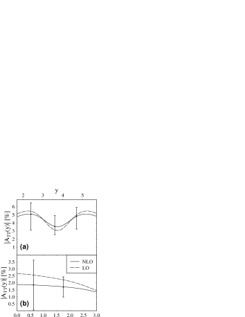
Figure 56: The Drell–Yan transverse double-spin asymmetry as a function of the virtual photon rapidity $y$ and of the dilepton invariant mass $M$, for two values of the c.m. energy: (a) $\sqrt{s}=40\,\text{GeV}$ (corresponding to HERA-$\vec{N}$) and (b) $\sqrt{s}=200\,\text{GeV}$ (corresponding to RHIC). The error bars represent the estimated statistical uncertainties of the two experiments. From [105].

9.1.2 Transverse single-spin asymmetries

In the early seventies data on single-spin asymmetries in inclusive pion hadroproduction [287, 288, 289] provoked a theoretical certain interest, as it was widely held that large effects could not be reproduced within the framework of perturbative QCD [6]. In 1991 the E704 experiment at Fermilab extended the results on large single-spin asymmetries in inclusive pion hadroproduction with a transversely polarised proton [290, 291] to higher $p_{T}$. These surprising results have prompted intensive theoretical work on the subject.

As a matter of fact, one year before the recent Fermilab measurements, Sivers had suggested that single-spin asymmetries could originate, at leading twist, from the intrinsic motion of quarks in the colliding protons [40, 41]. This idea was pursued by the authors of [181, 39], who pointed out that the Sivers effect is not forbidden by time-reversal invariance [17] provided one takes into account soft interactions in the initial state. In so doing, $T$-odd distribution functions are introduced (see Secs. 4.8 and 7.4.1).

A different mechanism was proposed by Collins [17]. It relies on the hypothesis of final-state interactions, which would allow polarised quarks with non-zero transverse momentum to fragment into an unpolarised hadron (the Collins effect already discussed in Secs. 6.5 and 7.4.1).

Finally, as seen in Sec. 7.4.1, another way to produce single-spin asymmetries is to assume the existence of a $T$-odd transverse polarisation distribution of quarks in the unpolarised initial-state hadron.

All the above effects manifest themselves at leading twist. We shall concentrate on the Collins mechanism, which appears, among the three hypothetical sources of single-spin asymmetries just mentioned, the likeliest one (as repeatedly stressed, initial-state interactions are definitely harder to unravel than final-state interactions).

Figure 57: Fit to the data on $A_{T}^{\pi}$ for the process $p^{\uparrow}p\to\pi{X}$ [290, 291] assuming that only the Collins effect is active; the upper, middle, and lower sets of data and curves refer to $\pi^{+}$, $\pi^{0}$ and $\pi^{-}$, respectively. From [26].

The Collins effect was investigated phenomenologically in [26], under the hypothesis that it is the only mechanism contributing to single-spin asymmetries. The authors of [26] propose a simple parametrisation for the Collins fragmentation function $\Delta_{T}^{0}D_{\pi/q}(z,\langle\kappa_{\perp}\rangle)$ (see Sec. 6.5 and note that in [26] a function $\Delta^{N}D_{\pi/q^{\uparrow}}$ is defined, which is related to our $\Delta_{T}^{0}D_{\pi/q}$ by $\Delta^{N}D_{\pi/q^{\uparrow}}=2\,\Delta_{T}^{0}D_{\pi/q}$):

$$\Delta_{T}^{0}D_{\pi/q}(z,\langle\kappa_{\perp}\rangle)=N\,\frac{\langle\kappa_{\perp}(z)\rangle}{M}\,z^{\alpha}(1-z)^{\beta}\,,$$ (9.1.2)

where $M=1\,\text{GeV}$ and it is assumed that $\Delta_{T}^{0}D_{\pi/q}$ is peaked around the average value $\langle\kappa_{\perp}\rangle\equiv\langle\mathchoice{\mbox{\boldmath$\displaystyle\kappa$\unboldmath}}{\mbox{\boldmath$\textstyle\kappa$\unboldmath}}{\mbox{\boldmath$\scriptstyle\kappa$\unboldmath}}{\mbox{\boldmath$\scriptscriptstyle\kappa$\unboldmath}}_{\perp}^{2}\rangle^{1/2}$. The $z$ dependence of $\langle\kappa_{\perp}(z)\rangle$ is obtained from a fit to LEP measurements of the transverse momentum of charged pions inside jets [292] (remember that $\mathchoice{\mbox{\boldmath$\displaystyle\kappa$\unboldmath}}{\mbox{\boldmath$\textstyle\kappa$\unboldmath}}{\mbox{\boldmath$\scriptstyle\kappa$\unboldmath}}{\mbox{\boldmath$\scriptscriptstyle\kappa$\unboldmath}}_{\perp}\simeq-\mathchoice{\mbox{\boldmath$\displaystyle P$\unboldmath}}{\mbox{\boldmath$\textstyle P$\unboldmath}}{\mbox{\boldmath$\scriptstyle P$\unboldmath}}{\mbox{\boldmath$\scriptscriptstyle P$\unboldmath}}_{h\perp}/z$ neglecting the intrinsic motion of quarks inside the target). Isospin and charge-conjugation invariance allows one to reconstruct the entire flavour structure of quark fragmentation into pions, giving the relations

$$\Delta_{T}^{0}D_{\pi^{+}/u}=\Delta_{T}^{0}D_{\pi^{-}/d}=\Delta_{T}^{0}D_{\pi^{+}/\mathchoice{\makebox[0.0pt][l]{$\displaystyle\kern 1.45834pt\overline{\kern-1.7014pt\phantom{d}}$}}{\makebox[0.0pt][l]{$\textstyle\kern 1.45834pt\overline{\kern-1.7014pt\phantom{d}}$}}{\makebox[0.0pt][l]{$\scriptstyle\kern 1.02083pt\overline{\kern-1.19098pt\phantom{d}}$}}{\makebox[0.0pt][l]{$\scriptscriptstyle\kern 0.72916pt\overline{\kern-0.8507pt\phantom{d}}$}}d}=\Delta_{T}^{0}D_{\pi^{-}/\mathchoice{\makebox[0.0pt][l]{$\displaystyle\kern 0.90417pt\overline{\kern-1.05487pt\phantom{u}}$}}{\makebox[0.0pt][l]{$\textstyle\kern 0.90417pt\overline{\kern-1.05487pt\phantom{u}}$}}{\makebox[0.0pt][l]{$\scriptstyle\kern 0.63292pt\overline{\kern-0.7384pt\phantom{u}}$}}{\makebox[0.0pt][l]{$\scriptscriptstyle\kern 0.45209pt\overline{\kern-0.52744pt\phantom{u}}$}}u}=\\ 2\Delta_{T}^{0}D_{\pi^{0}/u}=2\Delta_{T}^{0}D_{\pi^{0}/d}=2\Delta_{T}^{0}D_{\pi^{0}/\mathchoice{\makebox[0.0pt][l]{$\displaystyle\kern 1.45834pt\overline{\kern-1.7014pt\phantom{d}}$}}{\makebox[0.0pt][l]{$\textstyle\kern 1.45834pt\overline{\kern-1.7014pt\phantom{d}}$}}{\makebox[0.0pt][l]{$\scriptstyle\kern 1.02083pt\overline{\kern-1.19098pt\phantom{d}}$}}{\makebox[0.0pt][l]{$\scriptscriptstyle\kern 0.72916pt\overline{\kern-0.8507pt\phantom{d}}$}}d}=2\Delta_{T}^{0}D_{\pi^{0}/\mathchoice{\makebox[0.0pt][l]{$\displaystyle\kern 0.90417pt\overline{\kern-1.05487pt\phantom{u}}$}}{\makebox[0.0pt][l]{$\textstyle\kern 0.90417pt\overline{\kern-1.05487pt\phantom{u}}$}}{\makebox[0.0pt][l]{$\scriptstyle\kern 0.63292pt\overline{\kern-0.7384pt\phantom{u}}$}}{\makebox[0.0pt][l]{$\scriptscriptstyle\kern 0.45209pt\overline{\kern-0.52744pt\phantom{u}}$}}u}=\Delta_{T}^{0}D_{\pi/q}\,.$$ (9.1.3)

Only valence quarks in the incoming protons are considered in [26]. Their transverse polarisation distributions are taken to be proportional to the unpolarised distributions, according to

$$\Delta_{T}{u}(x)=P_{T}^{u/p}\,u(x)\,,\qquad\Delta_{T}{d}(x)=P_{T}^{d/p}\,d(x)\,,$$ (9.1.4)

where the transverse polarisation $P_{T}^{u/p}$ of the $u$ quark is set equal to $2/3$, as in the $\text{SU}(6)$ model, whereas the transverse polarisation of the $d$ quark is left as a free parameter. The result of the fit to the single-spin asymmetry data is shown in Fig. 57. Good agreement is obtained if $\Delta_{T}^{0}D_{\pi/q}$ the positivity constraint $|\Delta_{T}^{0}D_{\pi/q}|\leq{D}_{\pi/q}$ saturates at large $z$, otherwise the value of the single-spin asymmetry $A_{T}^{\pi}$ is too small at large $x_{F}$. It also turns out that the resulting transversity distribution of the $d$ quark violates the Soffer bound $2\,|\Delta_{T}{d}|\leq{d}+\Delta{d}$. Boglione and Leader pointed out [293] that, since $\Delta{d}$ is negative in most parametrisations, the Soffer constraint for the $d$ distributions is a rather strict one. A fit to the $A_{T}^{\pi}$ data that satisfies the Soffer inequality was performed in [293], with good results provided one allows $\Delta{d}$ to become positive at large $x$. In this case too, the positivity constraint on $\Delta_{T}^{0}D_{\pi/q}$ has to be saturated at large $z$. The inferred transversity distributions are shown in Fig. 58.

Figure 58: The transversity distributions obtained in [293] from a fit to the E704 data. The curves correspond to different parametrisations of the helicity distributions (see [293] for details). The figure is taken from [48].

Another calculation of the single-spin asymmetry in pion hadroproduction, based on the Collins effect, is presented in [294]. These authors generate the $T$-odd fragmentation function by the Lund string mechanism and obtain fair agreement with the E704 data by assuming the following behaviour for the transversity distributions:

$$\frac{\Delta_{T}{u}(x)}{u(x)}\simeq-\frac{\Delta_{T}{d}(x)}{d(x)}\to 1\,,\quad\text{as}\quad x\to 1\,.$$ (9.1.5)

A comment on the applicability of perturbative QCD to the analysis of the E704 measurements is in order. First of all, we have already pointed out that factorisation with intrinsic transverse momenta of quarks is not a proven property but only a (plausible) hypothesis. Second, and more important, the E704 data span a range of $|\mathchoice{\mbox{\boldmath$\displaystyle P$\unboldmath}}{\mbox{\boldmath$\textstyle P$\unboldmath}}{\mbox{\boldmath$\scriptstyle P$\unboldmath}}{\mbox{\boldmath$\scriptscriptstyle P$\unboldmath}}_{\pi\perp}|$ that reaches $4\,\text{GeV}$ for $\pi^{0}$ in the central region, where the asymmetry is small, and up to only $1.5\,\text{GeV}$ for $\pi^{\pm},\pi^{0}$ in the forward region, where the asymmetry is large. At such low values of transverse momenta perturbative QCD is not expected to be completely reliable, since cross-sections tend to rise very steeply as $|\mathchoice{\mbox{\boldmath$\displaystyle P$\unboldmath}}{\mbox{\boldmath$\textstyle P$\unboldmath}}{\mbox{\boldmath$\scriptstyle P$\unboldmath}}{\mbox{\boldmath$\scriptscriptstyle P$\unboldmath}}_{\pi\perp}|\to 0$. What allows some confidence that a perturbative QCD treatment is nevertheless meaningful is the fact that both intrinsic $\mathchoice{\mbox{\boldmath$\displaystyle\kappa$\unboldmath}}{\mbox{\boldmath$\textstyle\kappa$\unboldmath}}{\mbox{\boldmath$\scriptstyle\kappa$\unboldmath}}{\mbox{\boldmath$\scriptscriptstyle\kappa$\unboldmath}}_{\perp}$ effects and higher twists (see below) regularise the cross-sections at $\mathchoice{\mbox{\boldmath$\displaystyle P$\unboldmath}}{\mbox{\boldmath$\textstyle P$\unboldmath}}{\mbox{\boldmath$\scriptstyle P$\unboldmath}}{\mbox{\boldmath$\scriptscriptstyle P$\unboldmath}}_{\pi\perp}=0$.

A phenomenological analysis of the E704 results, based on the Sivers effect as the only source of single-spin asymmetries, was carried out in [181, 39]. For other (model) calculations of $A_{T}^{\pi}$ see [295, 296].

As shown in Sec. 7.4.2, single-spin asymmetries may also arise as a result of twist-three effects [175, 177, 182, 183]. Qiu and Sterman have used the first, chirally even, term of eq. (7.4.20) to fit the E704 data on $A_{T}^{\pi}$, setting

$$G_{F}(x,x)=K\,q(x)\,,$$ (9.1.6)

where $K$ is a constant parameter. Their fit is shown in Fig. 59.

Another twist-three contribution, the second term in eq. (7.4.20), involves the transversity distributions. This term has been evaluated by Kanazawa and Koike [182, 183] with an assumption similar to (9.1.6) for the multiparton distribution $E_{F}$, i.e.,

$$E_{F}(x,x)=K^{\prime}\,\Delta_{T}{q}(x)\,.$$ (9.1.7)

They found that, owing to the smallness of the hard partonic cross-sections, this chirally-odd contribution to single-spin asymmetries turns out to be negligible.

Clearly, in order to discriminate between leading-twist intrinsic $\mathchoice{\mbox{\boldmath$\displaystyle\kappa$\unboldmath}}{\mbox{\boldmath$\textstyle\kappa$\unboldmath}}{\mbox{\boldmath$\scriptstyle\kappa$\unboldmath}}{\mbox{\boldmath$\scriptscriptstyle\kappa$\unboldmath}}_{\perp}$ effects and higher-twist mechanisms a precise measurement of the $\mathchoice{\mbox{\boldmath$\displaystyle P$\unboldmath}}{\mbox{\boldmath$\textstyle P$\unboldmath}}{\mbox{\boldmath$\scriptstyle P$\unboldmath}}{\mbox{\boldmath$\scriptscriptstyle P$\unboldmath}}_{\pi\perp}$ dependence of the asymmetry is needed, in particular at large $\mathchoice{\mbox{\boldmath$\displaystyle P$\unboldmath}}{\mbox{\boldmath$\textstyle P$\unboldmath}}{\mbox{\boldmath$\scriptstyle P$\unboldmath}}{\mbox{\boldmath$\scriptscriptstyle P$\unboldmath}}_{\pi\perp}$. Given the current experimental information on $A_{T}^{\pi}$ it is just impossible to draw definite conclusions as to the dynamical source of single-spin transverse asymmetries.

Figure 59: The fit to the single-spin asymmetry data (here $A_{T}^{\pi}$ is called $A_{N}$) performed in [177].

9.2 Transverse polarisation in lepton–nucleon collisions

Let us turn now to semi-inclusive DIS on a transversely polarised proton. As discussed at length in Sec. 6, there are three candidate reactions for determining $\Delta_{T}{q}$ at leading twist:

1. semi-inclusive leptoproduction of a transversely polarised hadron with a transversely polarised target;

2. semi-inclusive leptoproduction of an unpolarised hadron with a transversely polarised target;

3. semi-inclusive leptoproduction of two hadrons with a transversely polarised target.

We shall review some calculations concerning the first two reactions. Two-hadron production is more difficult to predict, as it involves interference fragmentation functions for which we have at present no independent information from other processes (a model calculation is presented in [145]).

9.2.1 $\Lambda^{0}$ hyperon polarimetry

We have seen in Sec. 6.5 that detecting a transversely polarised hadron $h^{\uparrow}$ in the final state of a semi-inclusive DIS process with a transversely polarised target, $l\,p^{\uparrow}\to l^{\prime}\,h^{\uparrow}\,X$, probes the product $\Delta_{T}{q}(x)\,\Delta_{T}{D}_{q}(z)$ at leading twist. The relevant observable is the polarisation of $h^{\uparrow}$, which at lowest order reads (we take the $y$ axis as the polarisation axis)

$$\mathcal{P}_{y}^{h^{\uparrow}}=\hat{a}_{T}(t)\,\frac{\sum_{q,\mathchoice{\makebox[0.0pt][l]{$\displaystyle\kern 0.90417pt\overline{\kern-1.05487pt\phantom{q}}$}}{\makebox[0.0pt][l]{$\textstyle\kern 0.90417pt\overline{\kern-1.05487pt\phantom{q}}$}}{\makebox[0.0pt][l]{$\scriptstyle\kern 0.63292pt\overline{\kern-0.7384pt\phantom{q}}$}}{\makebox[0.0pt][l]{$\scriptscriptstyle\kern 0.45209pt\overline{\kern-0.52744pt\phantom{q}}$}}q}e_{q}^{2}\,\Delta_{T}{q}(x,Q^{2})\,\Delta_{T}{D}_{h/q}(z,Q^{2})}{\sum_{q,\mathchoice{\makebox[0.0pt][l]{$\displaystyle\kern 0.90417pt\overline{\kern-1.05487pt\phantom{q}}$}}{\makebox[0.0pt][l]{$\textstyle\kern 0.90417pt\overline{\kern-1.05487pt\phantom{q}}$}}{\makebox[0.0pt][l]{$\scriptstyle\kern 0.63292pt\overline{\kern-0.7384pt\phantom{q}}$}}{\makebox[0.0pt][l]{$\scriptscriptstyle\kern 0.45209pt\overline{\kern-0.52744pt\phantom{q}}$}}q}e_{q}^{2}\,q(x,Q^{2})\,D_{h/q}(z,Q^{2})}\,,$$ (9.2.1)

where $\hat{a}_{T}(y)=2(1-y)/[1+(1-y)^{2}]$ is the elementary transverse asymmetry (the QED depolarisation factor). In this class of reactions, the most promising is $\Lambda^{0}$ production. The $\Lambda^{0}$ polarisation is, in fact, easily measured by studying the angular distribution of the $\Lambda^{0}\to{p}\pi$ decay. The transverse polarisation of $\Lambda$’s produced in hard processes was studied a long time ago in [297, 298] and more recently in [126]. From the phenomenological viewpoint, the main problem is that, in order to compute the quantity (9.2.1), one needs to know the fragmentation functions $\Delta_{T}{D}_{h/q}(z,Q^{2})$ besides the transversity distributions.

A prediction for $\mathcal{P}_{y}^{\Lambda^{\uparrow}}$ has been recently presented by Anselmino, Boglione and Murgia [299]. These authors assume, at some starting scale $Q_{0}^{2}$, the relations

$$D_{\Lambda/u}=D_{\Lambda/d}=D_{\Lambda/s}=D_{\Lambda/{\mathchoice{\makebox[0.0pt][l]{$\displaystyle\kern 0.90417pt\overline{\kern-1.05487pt\phantom{u}}$}}{\makebox[0.0pt][l]{$\textstyle\kern 0.90417pt\overline{\kern-1.05487pt\phantom{u}}$}}{\makebox[0.0pt][l]{$\scriptstyle\kern 0.63292pt\overline{\kern-0.7384pt\phantom{u}}$}}{\makebox[0.0pt][l]{$\scriptscriptstyle\kern 0.45209pt\overline{\kern-0.52744pt\phantom{u}}$}}u}}=D_{\Lambda/{\mathchoice{\makebox[0.0pt][l]{$\displaystyle\kern 1.45834pt\overline{\kern-1.7014pt\phantom{d}}$}}{\makebox[0.0pt][l]{$\textstyle\kern 1.45834pt\overline{\kern-1.7014pt\phantom{d}}$}}{\makebox[0.0pt][l]{$\scriptstyle\kern 1.02083pt\overline{\kern-1.19098pt\phantom{d}}$}}{\makebox[0.0pt][l]{$\scriptscriptstyle\kern 0.72916pt\overline{\kern-0.8507pt\phantom{d}}$}}d}}=D_{\Lambda/{\mathchoice{\makebox[0.0pt][l]{$\displaystyle\kern 0.90417pt\overline{\kern-1.05487pt\phantom{s}}$}}{\makebox[0.0pt][l]{$\textstyle\kern 0.90417pt\overline{\kern-1.05487pt\phantom{s}}$}}{\makebox[0.0pt][l]{$\scriptstyle\kern 0.63292pt\overline{\kern-0.7384pt\phantom{s}}$}}{\makebox[0.0pt][l]{$\scriptscriptstyle\kern 0.45209pt\overline{\kern-0.52744pt\phantom{s}}$}}s}}\equiv D_{\Lambda/q}\,,$$ (9.2.2a)

$$\Delta_{T}{D}_{\Lambda/u}=\Delta_{T}{D}_{\Lambda/d}=\Delta_{T}{D}_{\Lambda/{\mathchoice{\makebox[0.0pt][l]{$\displaystyle\kern 0.90417pt\overline{\kern-1.05487pt\phantom{u}}$}}{\makebox[0.0pt][l]{$\textstyle\kern 0.90417pt\overline{\kern-1.05487pt\phantom{u}}$}}{\makebox[0.0pt][l]{$\scriptstyle\kern 0.63292pt\overline{\kern-0.7384pt\phantom{u}}$}}{\makebox[0.0pt][l]{$\scriptscriptstyle\kern 0.45209pt\overline{\kern-0.52744pt\phantom{u}}$}}u}}=\Delta_{T}{D}_{\Lambda/{\mathchoice{\makebox[0.0pt][l]{$\displaystyle\kern 1.45834pt\overline{\kern-1.7014pt\phantom{d}}$}}{\makebox[0.0pt][l]{$\textstyle\kern 1.45834pt\overline{\kern-1.7014pt\phantom{d}}$}}{\makebox[0.0pt][l]{$\scriptstyle\kern 1.02083pt\overline{\kern-1.19098pt\phantom{d}}$}}{\makebox[0.0pt][l]{$\scriptscriptstyle\kern 0.72916pt\overline{\kern-0.8507pt\phantom{d}}$}}d}}=N\,\Delta_{T}{D}_{\Lambda/s}=N\,\Delta{D}_{\Lambda/s}\,,$$ (9.2.2b)

where $N$ is a free parameter. For $D_{\Lambda/q}$ and $\Delta{D}_{\Lambda/s}$ they use the parametrisation of [300] at $Q_{0}^{2}=0.23\,\text{GeV}^{2}$. As for the transversity distributions, saturation of the Soffer bound is assumed and sea densities are neglected. Leading-order QCD evolution is applied. In Fig. 60 we show the results of [299] for $\mathcal{P}_{y}^{\Lambda^{\uparrow}}$, with three different choices of $N$ and $\alpha$: the first scenario corresponds to the $\text{SU}(6)$ non-relativistic quark model (the entire spin of the $\Lambda^{0}$ is carried by the strange quark, i.e., $N=0$); the second scenario corresponds to a negative $N$; and the third scenario corresponds to all light quarks contributing equally to the $\Lambda^{0}$ spin (i.e., $N=1$). Other predictions for the $\Lambda^{0}$ polarisation are offered by Ma et al. [318].

Figure 60: The polarisation of $\Lambda^{0}$ hyperons produced in semi-inclusive DIS, as predicted in [299].

9.2.2 Azimuthal asymmetries in pion leptoproduction

A potentially relevant reaction for the study of transversity is leptoproduction of unpolarised hadrons (typically pions) with a transversely polarised target, $l\,p^{\uparrow}\to{l^{\prime}}\,h\,X$. In this case, as seen in Sec. 6.5, $\Delta_{T}{q}$ may be probed as a consequence of the Collins effect (a $T$-odd contribution to quark fragmentation arising from final-state interactions). In this case one essentially measures $\Delta_{T}{q}(x)\,H_{1}^{{\perp}q}(z,\mathchoice{\mbox{\boldmath$\displaystyle P$\unboldmath}}{\mbox{\boldmath$\textstyle P$\unboldmath}}{\mbox{\boldmath$\scriptstyle P$\unboldmath}}{\mbox{\boldmath$\scriptscriptstyle P$\unboldmath}}_{h\perp}^{2})$.

Preliminary results on single-spin transverse asymmetries in pion leptoproduction have been recently reported by the SMC [24] and the HERMES collaboration [23]. Before presenting them, we return to a kinematical problem already addressed in Sec. 3.1: the definition of the target polarisation.

Figure 61: The target spin and the lepton and photon momenta. Note that $\textstyle q$ is directed along the negative $z$ axis.

From the experimental point of view, the DIS target is “longitudinally” (“transversely”) polarised when its spin $\textstyle S$ is parallel (perpendicular) to the initial lepton momentum $\textstyle\ell$. If we parametrise $\textstyle S$ as (see Fig. 61)

$$\mathchoice{\mbox{\boldmath$\displaystyle S$\unboldmath}}{\mbox{\boldmath$\textstyle S$\unboldmath}}{\mbox{\boldmath$\scriptstyle S$\unboldmath}}{\mbox{\boldmath$\scriptscriptstyle S$\unboldmath}}=|\mathchoice{\mbox{\boldmath$\displaystyle S$\unboldmath}}{\mbox{\boldmath$\textstyle S$\unboldmath}}{\mbox{\boldmath$\scriptstyle S$\unboldmath}}{\mbox{\boldmath$\scriptscriptstyle S$\unboldmath}}|\,(\sin\vartheta_{S}\,\cos\phi_{S},\,-\sin\vartheta_{S}\,\sin\phi_{S},\,-\cos\vartheta_{S})\,,$$ (9.2.3)

and $\textstyle\ell$ as

$$\mathchoice{\mbox{\boldmath$\displaystyle\ell$\unboldmath}}{\mbox{\boldmath$\textstyle\ell$\unboldmath}}{\mbox{\boldmath$\scriptstyle\ell$\unboldmath}}{\mbox{\boldmath$\scriptscriptstyle\ell$\unboldmath}}=E\,(\sin\vartheta_{\gamma},\,0,\,-\cos\vartheta_{\gamma})\,,$$ (9.2.4)

the angle $\alpha$ between $\textstyle S$ and $\textstyle\ell$ is given by

$$\cos\alpha=\sin\vartheta_{\gamma}\,\sin\vartheta_{S}\,\cos\phi_{S}+\cos\vartheta_{\gamma}\,\cos\vartheta_{S}\,.$$ (9.2.5)

Thus, we have

$$\begin{array}[]{l@{\quad}c@{\quad}l}\alpha=0&\Rightarrow&\text{``longitudinal'' polarisation}\,,\\ \alpha=\frac{\pi}{2}&\Rightarrow&\text{``transverse'' polarisation}\,.\end{array}$$

We use quotation marks when adopting the experimental terminology.

From the theoretical point of view, it is more convenient to focus on the target and ignore the leptons. Thus the target is said to be longitudinal (transverse) polarised when its spin is parallel (perpendicular) to the photon momentum, i.e.,

$$\begin{array}[]{l@{\quad}c@{\quad}l}\vartheta_{S}=0&\Rightarrow&\text{longitudinal polarisation}\,,\\ \vartheta_{S}=\frac{\pi}{2}&\Rightarrow&\text{transverse polarisation}\,.\end{array}$$

The absence of quotation marks signals the theoretical terminology.

DIS kinematics gives

$$\sin\vartheta_{\gamma} = \frac{2Mx}{Q}\,\sqrt{1-y}+\mathop{\mathcal{O}}\nolimits(M^{3}/Q^{3})\,,$$ (9.2.6a)

$$\cos\vartheta_{\gamma} = 1-\frac{2M^{2}x^{2}}{Q^{2}}\,(1-y)+\mathop{\mathcal{O}}\nolimits(M^{4}/Q^{4})\,,$$ (9.2.6b)

and inverting (9.2.5) we obtain

$$\cos\vartheta_{S} \simeq \cos\alpha-\frac{2Mx}{Q}\,\sqrt{1-y}\,\sin\alpha\,\cos\phi_{S}\,,$$ (9.2.7a)

$$\sin\vartheta_{S} \simeq \sin\alpha+\frac{2Mx}{Q}\,\sqrt{1-y}\,\cos\alpha\,\cos\phi_{S}\,,$$ (9.2.7b)

where we have neglected $\mathop{\mathcal{O}}\nolimits(M^{2}/Q^{2})$ terms.

If the target is “longitudinally” polarised (i.e., $\alpha=0$), one has

$$\cos\vartheta_{S} \simeq 1\,,$$ (9.2.8a)

$$\sin\vartheta_{S} \simeq \frac{2Mx}{Q}\,\sqrt{1-y}\,\cos\phi_{S}\,,$$ (9.2.8b)

so that (setting $\phi_{S}=0$ since the lepton momenta lie in the $xz$ plane)

$$|\mathchoice{\mbox{\boldmath$\displaystyle S$\unboldmath}}{\mbox{\boldmath$\textstyle S$\unboldmath}}{\mbox{\boldmath$\scriptstyle S$\unboldmath}}{\mbox{\boldmath$\scriptscriptstyle S$\unboldmath}}_{\perp}|\simeq\frac{2Mx}{Q}\,\sqrt{1-y}\,|\mathchoice{\mbox{\boldmath$\displaystyle S$\unboldmath}}{\mbox{\boldmath$\textstyle S$\unboldmath}}{\mbox{\boldmath$\scriptstyle S$\unboldmath}}{\mbox{\boldmath$\scriptscriptstyle S$\unboldmath}}|\,.$$ (9.2.9)

Therefore, when the target is “longitudinally” polarised, its spin has a non-zero transverse component, suppressed by a factor $1/Q$. This means that there is a transverse single-spin asymmetry given by (see (6.5.10))

$$A_{T}^{\pi} \simeq \hat{a}_{T}(y)\,\frac{\sum_{a}e_{a}^{2}\,\Delta_{T}{f}_{a}(x)\,\Delta_{T}^{0}D_{a}(z,\mathchoice{\mbox{\boldmath$\displaystyle P$\unboldmath}}{\mbox{\boldmath$\textstyle P$\unboldmath}}{\mbox{\boldmath$\scriptstyle P$\unboldmath}}{\mbox{\boldmath$\scriptscriptstyle P$\unboldmath}}_{h\perp}^{2})}{\sum_{a}e_{a}^{2}\,f_{a}(x)\,D_{a}(z,\mathchoice{\mbox{\boldmath$\displaystyle P$\unboldmath}}{\mbox{\boldmath$\textstyle P$\unboldmath}}{\mbox{\boldmath$\scriptstyle P$\unboldmath}}{\mbox{\boldmath$\scriptscriptstyle P$\unboldmath}}_{h\perp}^{2})}$$ (9.2.10)

$$\hbox{}\times|\mathchoice{\mbox{\boldmath$\displaystyle S$\unboldmath}}{\mbox{\boldmath$\textstyle S$\unboldmath}}{\mbox{\boldmath$\scriptstyle S$\unboldmath}}{\mbox{\boldmath$\scriptscriptstyle S$\unboldmath}}|\,\frac{2Mx}{Q}\,\sqrt{1-y}\,\sin\phi_{\pi}\,.$$

We stress that the $1/Q$ factor in (9.2.10), which mimics a twist-three contribution, has a purely kinematical origin. This is the situation explored by HERMES [23].

If the target is “transversely” polarised (i.e., $\alpha=\pi/2$), one has

$$\cos\vartheta_{S} \simeq -\frac{2Mx}{Q}\,\sqrt{1-y}\,\cos\phi_{S}\,,$$ (9.2.11a)

$$\sin\vartheta_{S} \simeq 1\,,$$ (9.2.11b)

and

$$|\mathchoice{\mbox{\boldmath$\displaystyle S$\unboldmath}}{\mbox{\boldmath$\textstyle S$\unboldmath}}{\mbox{\boldmath$\scriptstyle S$\unboldmath}}{\mbox{\boldmath$\scriptscriptstyle S$\unboldmath}}_{\perp}|\simeq|\mathchoice{\mbox{\boldmath$\displaystyle S$\unboldmath}}{\mbox{\boldmath$\textstyle S$\unboldmath}}{\mbox{\boldmath$\scriptstyle S$\unboldmath}}{\mbox{\boldmath$\scriptscriptstyle S$\unboldmath}}|\,.$$ (9.2.12)

In this case, neglecting $1/Q^{2}$ kinematical effects, the target is also transversely polarised; the measured transverse single-spin asymmetry is unsuppressed and is given by eq. (6.5.10). This is the situation of the SMC experiment [24].

Figure 62: The SMC data [24] on the transverse single-spin asymmetry in pion leptoproduction, as a function of the Collins angle.

Let us now come to the data. The SMC [24] presented a preliminary measurement of $A_{T}^{\pi}$ for pion production in DIS of unpolarised muons off a transversely polarised proton target at $s=188.5\,\text{GeV}^{2}$ and

$$\langle x\rangle\simeq 0.08\,,\quad\langle y\rangle\simeq 0.33\,,\quad\langle z\rangle\simeq 0.45\,,\quad\langle Q^{2}\rangle\simeq 5\,\text{GeV}^{2}\,.$$ (9.2.13)

Two data sets, with $\langle\mathchoice{\mbox{\boldmath$\displaystyle P$\unboldmath}}{\mbox{\boldmath$\textstyle P$\unboldmath}}{\mbox{\boldmath$\scriptstyle P$\unboldmath}}{\mbox{\boldmath$\scriptscriptstyle P$\unboldmath}}_{\pi\perp}\rangle=0.5\,\text{GeV}$ and $\langle\mathchoice{\mbox{\boldmath$\displaystyle P$\unboldmath}}{\mbox{\boldmath$\textstyle P$\unboldmath}}{\mbox{\boldmath$\scriptstyle P$\unboldmath}}{\mbox{\boldmath$\scriptscriptstyle P$\unboldmath}}_{\pi\perp}\rangle=0.8\,\text{GeV}$, are selected. The result for the total amount of events is (note that SMC use a different choice of axes and, moreover, their Collins angle has the opposite sign with respect to ours)

$$A_{T}^{\pi^{+}}/\hat{a}_{T} = \hphantom{-}(0.11\pm 0.06)\,\sin(\phi_{\pi}+\phi_{S})\,,$$ (9.2.14a)

$$A_{T}^{\pi^{-}}/\hat{a}_{T} = -(0.02\pm 0.06)\,\sin(\phi_{\pi}+\phi_{S})\,.$$ (9.2.14b)

The SMC data are shown in Fig. 62.

Evaluating the depolarisation factor $\hat{a}_{T}$ at $\langle{y}\rangle\simeq 0.33$, eqs. (9.2.14a, LABEL:subpion12) imply

$$A_{T}^{\pi^{+}} = \hphantom{-}(0.10\pm 0.06)\,\sin(\phi_{\pi}+\phi_{S}),$$ (9.2.15a)

$$A_{T}^{\pi^{-}} = -(0.02\pm 0.06)\,\sin(\phi_{\pi}+\phi_{S})\,.$$ (9.2.15b)

The HERMES experiment at HERA [23] has reported results on $A_{T}^{\pi}$ for positive and negative pions produced in DIS of unpolarised positrons off a “longitudinally” polarised proton target at $s=52.6\,\text{GeV}^{2}$ and in the kinematical ranges:

$$0.023\leq x\leq 0.4\,,\quad 0.1\leq y\leq 0.85\,,\quad 0.2\leq z\leq 0.7\,,\quad Q^{2}\geq 1\,\text{GeV}^{2}\,.$$ (9.2.16)

The transverse momentum of the produced pions is $|\mathchoice{\mbox{\boldmath$\displaystyle P$\unboldmath}}{\mbox{\boldmath$\textstyle P$\unboldmath}}{\mbox{\boldmath$\scriptstyle P$\unboldmath}}{\mbox{\boldmath$\scriptscriptstyle P$\unboldmath}}_{\pi\perp}|\lesssim 1\,\text{GeV}$. The HERMES result is (see Fig. 63)

$$A_{T}^{\pi^{+}} = +\left[0.022\pm 0.004\,(\text{stat.})\pm 0.004\,(\text{syst.})\right]\sin\phi_{\pi}\,,$$ (9.2.17a)

$$A_{T}^{\pi^{-}} = -\left[0.001\pm 0.005\,(\text{stat.})\pm 0.004\,(\text{syst.})\right]\sin\phi_{\pi}\,.$$ (9.2.17b)

The conventions for the axes and the Collins angle used by HERMES are the same as ours. There appears to be a sign difference between the SMC and HERMES results. Unfortunately, the proliferation of conventions does not help to settle sign problems. According to the discussion above, the HERMES data, which are obtained with a “longitudinally” polarised target, gives a transverse single-spin asymmetry suppressed by $1/Q$. Thus, higher-twist longitudinal effects might be as relevant as the leading-twist Collins effect. The result (9.2.17a), (9.2.17b) should be taken with this caveat in mind. Another, even deeper, reason to be very cautious in interpreting the SMC and HERMES results is the low values of $\langle|\mathchoice{\mbox{\boldmath$\displaystyle P$\unboldmath}}{\mbox{\boldmath$\textstyle P$\unboldmath}}{\mbox{\boldmath$\scriptstyle P$\unboldmath}}{\mbox{\boldmath$\scriptscriptstyle P$\unboldmath}}_{\pi\perp}|\rangle$ covered by the two experiments. This renders any perturbative QCD analysis rather problematic.

Anselmino and Murgia [301] have recently analysed the SMC and HERMES data and extracted bounds on the Collins fragmentation function $\Delta_{T}^{0}D_{\pi/q}$ (for another analysis see [319]). They simplify the expression of the single-spin transverse asymmetry (6.5.10) by assuming that the transversity of the sea is negligible, i.e., $\Delta_{T}\mathchoice{\makebox[0.0pt][l]{$\displaystyle\kern 1.29167pt\overline{\kern-1.50696pt\phantom{q}}$}}{\makebox[0.0pt][l]{$\textstyle\kern 1.29167pt\overline{\kern-1.50696pt\phantom{q}}$}}{\makebox[0.0pt][l]{$\scriptstyle\kern 0.90417pt\overline{\kern-1.05487pt\phantom{q}}$}}{\makebox[0.0pt][l]{$\scriptscriptstyle\kern 0.64583pt\overline{\kern-0.75348pt\phantom{q}}$}}q\simeq 0$, using eqs. (9.1.3) for the fragmentation functions into pions and similar relations for $D_{\pi/q}$, and ignoring the non-valence quark contributions in pions. Thus, the single-spin transverse asymmetries become

$$A_{T}^{\pi^{+}} \sim \frac{4\Delta_{T}{u}(x)}{4u(x)+\mathchoice{\makebox[0.0pt][l]{$\displaystyle\kern 2.08334pt\overline{\kern-2.43059pt\phantom{d}}$}}{\makebox[0.0pt][l]{$\textstyle\kern 2.08334pt\overline{\kern-2.43059pt\phantom{d}}$}}{\makebox[0.0pt][l]{$\scriptstyle\kern 1.45834pt\overline{\kern-1.7014pt\phantom{d}}$}}{\makebox[0.0pt][l]{$\scriptscriptstyle\kern 1.04167pt\overline{\kern-1.21529pt\phantom{d}}$}}d(x)}\,\frac{\Delta_{T}^{0}D_{\pi/q}(z,P_{\pi\perp})}{D_{\pi/q}(z,P_{\pi\perp})}\,,$$ (9.2.18a)

$$A_{T}^{\pi^{-}} \sim \frac{\Delta_{T}{d}(x)}{d(x)+4\mathchoice{\makebox[0.0pt][l]{$\displaystyle\kern 1.29167pt\overline{\kern-1.50696pt\phantom{u}}$}}{\makebox[0.0pt][l]{$\textstyle\kern 1.29167pt\overline{\kern-1.50696pt\phantom{u}}$}}{\makebox[0.0pt][l]{$\scriptstyle\kern 0.90417pt\overline{\kern-1.05487pt\phantom{u}}$}}{\makebox[0.0pt][l]{$\scriptscriptstyle\kern 0.64583pt\overline{\kern-0.75348pt\phantom{u}}$}}u(x)}\,\frac{\Delta_{T}^{0}D_{\pi/q}(z,P_{\pi\perp})}{D_{\pi/q}(z,P_{\pi\perp})}\,,$$ (9.2.18b)

$$A_{T}^{\pi^{0}} \sim \frac{4\Delta_{T}{u}(x)+\Delta_{T}{d}(x)}{4u(x)+d(x)+4\mathchoice{\makebox[0.0pt][l]{$\displaystyle\kern 1.29167pt\overline{\kern-1.50696pt\phantom{u}}$}}{\makebox[0.0pt][l]{$\textstyle\kern 1.29167pt\overline{\kern-1.50696pt\phantom{u}}$}}{\makebox[0.0pt][l]{$\scriptstyle\kern 0.90417pt\overline{\kern-1.05487pt\phantom{u}}$}}{\makebox[0.0pt][l]{$\scriptscriptstyle\kern 0.64583pt\overline{\kern-0.75348pt\phantom{u}}$}}u(x)+\mathchoice{\makebox[0.0pt][l]{$\displaystyle\kern 2.08334pt\overline{\kern-2.43059pt\phantom{d}}$}}{\makebox[0.0pt][l]{$\textstyle\kern 2.08334pt\overline{\kern-2.43059pt\phantom{d}}$}}{\makebox[0.0pt][l]{$\scriptstyle\kern 1.45834pt\overline{\kern-1.7014pt\phantom{d}}$}}{\makebox[0.0pt][l]{$\scriptscriptstyle\kern 1.04167pt\overline{\kern-1.21529pt\phantom{d}}$}}d(x)}\,\frac{\Delta_{T}^{0}D_{\pi/q}(z,P_{\pi\perp})}{D_{\pi/q}(z,P_{\pi\perp})}\,.$$ (9.2.18c)

Saturating the Soffer inequality, the authors of [301] derive a lower bound for the quark analysing power $\Delta_{T}^{0}D_{\pi/q}/D_{\pi/q}$ from the data on $A_{T}^{\pi}$. From the SMC result they find

$$\frac{|\Delta_{T}^{0}D_{\pi/q}|}{D_{\pi/q}}\gtrsim 0.24\pm 0.15\,,\quad\langle z\rangle\simeq 0.45\,,\quad\langle P_{\pi\perp}\rangle\simeq 0.65\,\text{GeV}\,,$$ (9.2.19a)

and from the HERMES data

$$\frac{|\Delta_{T}^{0}D_{\pi/q}|}{D_{\pi/q}}\gtrsim 0.20\pm 0.04\,(\text{stat.})\pm 0.04\,(\text{syst.})\,,\quad z\geq 0.2\,.$$ (9.2.19b)

These results, if confirmed, would indicate a large value of the Collins fragmentation function and would therefore also point to a relevant contribution of the Collins effect in other processes. More data at higher $\mathchoice{\mbox{\boldmath$\displaystyle P$\unboldmath}}{\mbox{\boldmath$\textstyle P$\unboldmath}}{\mbox{\boldmath$\scriptstyle P$\unboldmath}}{\mbox{\boldmath$\scriptscriptstyle P$\unboldmath}}_{\pi\perp}$ would clearly make a perturbative QCD study definitely safer. For another determination of the Collins analysing power see below, Sec. 9.3.

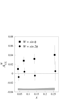
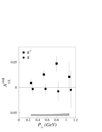
Figure 63: The HERMES data [23] on the transverse single-spin asymmetry in pion leptoproduction, as a function of $x$ (left) and $|\mathchoice{\mbox{\boldmath$\displaystyle P$\unboldmath}}{\mbox{\boldmath$\textstyle P$\unboldmath}}{\mbox{\boldmath$\scriptstyle P$\unboldmath}}{\mbox{\boldmath$\scriptscriptstyle P$\unboldmath}}_{\pi\perp}|$ (right).

As already recalled, the interpretation of the HERMES result is made difficult by the fact that the target is “longitudinally” polarised (that is $|\mathchoice{\mbox{\boldmath$\displaystyle S$\unboldmath}}{\mbox{\boldmath$\textstyle S$\unboldmath}}{\mbox{\boldmath$\scriptstyle S$\unboldmath}}{\mbox{\boldmath$\scriptscriptstyle S$\unboldmath}}_{\perp}|\sim\frac{M}{Q}\,|\mathchoice{\mbox{\boldmath$\displaystyle S$\unboldmath}}{\mbox{\boldmath$\textstyle S$\unboldmath}}{\mbox{\boldmath$\scriptstyle S$\unboldmath}}{\mbox{\boldmath$\scriptscriptstyle S$\unboldmath}}|$ and $|\mathchoice{\mbox{\boldmath$\displaystyle S$\unboldmath}}{\mbox{\boldmath$\textstyle S$\unboldmath}}{\mbox{\boldmath$\scriptstyle S$\unboldmath}}{\mbox{\boldmath$\scriptscriptstyle S$\unboldmath}}_{\parallel}|\sim|\mathchoice{\mbox{\boldmath$\displaystyle S$\unboldmath}}{\mbox{\boldmath$\textstyle S$\unboldmath}}{\mbox{\boldmath$\scriptstyle S$\unboldmath}}{\mbox{\boldmath$\scriptscriptstyle S$\unboldmath}}|$). Thus, focusing on the dominant $1/Q$ effects, there are in principle two types of contributions to the cross-section: 1) leading-twist contributions for a transversely polarised target; 2) twist-three contributions for a longitudinally polarised target. Type 1 is $\mathop{\mathcal{O}}\nolimits(1/Q)$ owing to the kinematical relation (9.2.9); type 2 is $\mathop{\mathcal{O}}\nolimits(1/Q)$ owing to dynamical twist-three effects. The $\sin\phi_{\pi}$ asymmetry measured by HERMES receives the following contributions [121, 15, 133, 302, 303, 304, 305, 48] (we omit the factors in front of each term):

$$A_{\sin\phi_{h}}^{\pi} \sim |\mathchoice{\mbox{\boldmath$\displaystyle S$\unboldmath}}{\mbox{\boldmath$\textstyle S$\unboldmath}}{\mbox{\boldmath$\scriptstyle S$\unboldmath}}{\mbox{\boldmath$\scriptscriptstyle S$\unboldmath}}_{\perp}|\,\Delta_{T}{q}\otimes H_{1}^{\perp(1)}+\frac{M}{Q}\,|\mathchoice{\mbox{\boldmath$\displaystyle S$\unboldmath}}{\mbox{\boldmath$\textstyle S$\unboldmath}}{\mbox{\boldmath$\scriptstyle S$\unboldmath}}{\mbox{\boldmath$\scriptscriptstyle S$\unboldmath}}_{\parallel}|\,h_{L}\otimes H_{1}^{\perp(1)}+\frac{M_{h}}{Q}\,|\mathchoice{\mbox{\boldmath$\displaystyle S$\unboldmath}}{\mbox{\boldmath$\textstyle S$\unboldmath}}{\mbox{\boldmath$\scriptstyle S$\unboldmath}}{\mbox{\boldmath$\scriptscriptstyle S$\unboldmath}}_{\parallel}|\,h_{1L}^{\perp(1)}\otimes\widetilde{H}$$

$$\sim \frac{M}{Q}\,|\mathchoice{\mbox{\boldmath$\displaystyle S$\unboldmath}}{\mbox{\boldmath$\textstyle S$\unboldmath}}{\mbox{\boldmath$\scriptstyle S$\unboldmath}}{\mbox{\boldmath$\scriptscriptstyle S$\unboldmath}}|\,\Delta_{T}{q}\otimes H_{1}^{\perp(1)}+\frac{M}{Q}\,|\mathchoice{\mbox{\boldmath$\displaystyle S$\unboldmath}}{\mbox{\boldmath$\textstyle S$\unboldmath}}{\mbox{\boldmath$\scriptstyle S$\unboldmath}}{\mbox{\boldmath$\scriptscriptstyle S$\unboldmath}}|\,h_{L}\otimes H_{1}^{\perp(1)}+\frac{M_{h}}{Q}\,|\mathchoice{\mbox{\boldmath$\displaystyle S$\unboldmath}}{\mbox{\boldmath$\textstyle S$\unboldmath}}{\mbox{\boldmath$\scriptstyle S$\unboldmath}}{\mbox{\boldmath$\scriptscriptstyle S$\unboldmath}}|\,h_{1L}^{\perp(1)}\otimes\widetilde{H}\,,$$

where $h_{1L}^{\perp(1)}$ and $H_{1}^{\perp(1)}$ are defined in (4.9.5a) and (6.5.22) respectively. The first term in (LABEL:pion25) is the type 1 term described above and corresponds to the Collins effect studied in [301]. The other two terms (type 2) were phenomenologically investigated in [302, 303, 304, 305, 48]. In order to analyse the data by means of (LABEL:pion25), extra input is needed, given the number of unknown quantities involved. As we have seen in Sec. 6.5, when the target is longitudinally polarised there is also a $\sin 2\phi_{h}$ asymmetry, which appears at leading twist and has the form

$$A_{\sin 2\phi_{\pi}}^{\pi}\sim|\mathchoice{\mbox{\boldmath$\displaystyle S$\unboldmath}}{\mbox{\boldmath$\textstyle S$\unboldmath}}{\mbox{\boldmath$\scriptstyle S$\unboldmath}}{\mbox{\boldmath$\scriptscriptstyle S$\unboldmath}}_{\parallel}|\,h_{1L}^{\perp(1)}\otimes H_{1}^{\perp(1)}\,.$$ (9.2.21)

The smallness of $A_{\sin 2\phi_{\pi}}^{\pi}$, as measured by HERMES (see Fig. 63), seems to be an indication in favour of $h_{1L}^{\perp(1)}\simeq 0$. If we make this assumption [303], recalling (4.10.1) and (4.10.2), we obtain $\widetilde{h}_{L}(x)=h_{L}(x)=\Delta_{T}{q}(x)$ and (LABEL:pion25) reduces to a single term of the type $\Delta_{T}{q}\otimes H_{1}^{\perp(1)}$. Using a simple parametrisation [17] for the Collins fragmentation function, namely

$$\frac{H_{1}^{\perp}(x,\mathchoice{\mbox{\boldmath$\displaystyle\kappa$\unboldmath}}{\mbox{\boldmath$\textstyle\kappa$\unboldmath}}{\mbox{\boldmath$\scriptstyle\kappa$\unboldmath}}{\mbox{\boldmath$\scriptscriptstyle\kappa$\unboldmath}}_{\perp}^{2})}{D(x,\mathchoice{\mbox{\boldmath$\displaystyle\kappa$\unboldmath}}{\mbox{\boldmath$\textstyle\kappa$\unboldmath}}{\mbox{\boldmath$\scriptstyle\kappa$\unboldmath}}{\mbox{\boldmath$\scriptscriptstyle\kappa$\unboldmath}}_{\perp}^{2})}=\frac{M_{h}\,M_{C}}{M_{C}^{2}+\mathchoice{\mbox{\boldmath$\displaystyle\kappa$\unboldmath}}{\mbox{\boldmath$\textstyle\kappa$\unboldmath}}{\mbox{\boldmath$\scriptstyle\kappa$\unboldmath}}{\mbox{\boldmath$\scriptscriptstyle\kappa$\unboldmath}}_{\perp}^{2}}\,,$$ (9.2.22)

with $M_{C}$ as a free parameter, the authors of [303] fit the HERMES data fairly well (see Fig. 64).

Figure 64: The single-spin azimuthal asymmetry in pion leptoproduction as computed in [303], compared to the HERMES data [23]. The solid line corresponds to $\Delta_{T}{q}=\Delta{q}$. The dashed line corresponds to saturation of the Soffer inequality.

In [48] it was pointed out that the HERMES data on the $\sin 2\phi_{\pi}$ asymmetry do not necessarily imply $h_{1L}^{\perp(1)}=0$. If one assumes the interaction-dependent distribution $\widetilde{h}_{L}(x)$ to be vanishing, so that from (4.9.5a) and (4.10.2) one has (neglecting quark mass terms)

$$h_{1L}^{\perp(1)}(x)=-\frac{1}{2}\,xh_{L}(x)=-x^{2}\int_{x}^{1}\!\frac{\d{y}}{y^{2}}\,\Delta_{T}{q}(y)\,,$$ (9.2.23)

then it is still possible to obtain a $\sin\phi_{\pi}$ asymmetry of the order of few percent (as found by HERMES), with the $\sin 2\phi_{\pi}$ asymmetry suppressed by a factor 2.

The approximation (9.2.23) was also adopted in [306], where an analysis of the HERMES and SMC data in the framework of the chiral quark–soliton model is presented.

In conclusion, we can say that the interpretation of the HERMES and SMC measurements is far from clear. The experimental results seem to indicate that transversity plays some rôle but the present scarcity of data, their errors, our ignorance of most of the quantities involved in the process, and, last but not least, uncertainty in the theoretical procedures make the entire matter still rather vague. More, and more precise, data will be of great help in settling the question.

9.3 Transverse polarisation in $e^{+}e^{-}$ collisions.

An independent source of information on the Collins fragmentation function $H_{1}^{\perp}$ is inclusive two-hadron production in electron–positron collisions (see Fig. 65):

$$e^{+}\,e^{-}\to h_{1}\,h_{2}\,X\,.$$ (9.3.1)

This process was studied in [307, 308, 309]. It turns out that the cross-section has the following angular dependence (we assume that two alike hadrons are produced, omit the flavour indices and refer to Fig. 65 for the kinematical variables)

$$\frac{\d\sigma}{\d\cos\theta_{2}\d\phi_{1}} \propto (1+\cos^{2}\theta_{2})\,D(z_{1})\mathchoice{\makebox[0.0pt][l]{$\displaystyle\kern 2.05pt\overline{\kern-2.3917pt\phantom{D}}$}}{\makebox[0.0pt][l]{$\textstyle\kern 2.05pt\overline{\kern-2.3917pt\phantom{D}}$}}{\makebox[0.0pt][l]{$\scriptstyle\kern 1.435pt\overline{\kern-1.67418pt\phantom{D}}$}}{\makebox[0.0pt][l]{$\scriptscriptstyle\kern 1.025pt\overline{\kern-1.19585pt\phantom{D}}$}}D(z_{2})$$ (9.3.2)

$$\hbox{}+C\,\sin^{2}\theta_{2}\,\cos(2\phi_{1})\,H_{1}^{\perp(1)}(z_{1})\mathchoice{\makebox[0.0pt][l]{$\displaystyle\kern 2.05pt\overline{\kern-2.3917pt\phantom{H}}$}}{\makebox[0.0pt][l]{$\textstyle\kern 2.05pt\overline{\kern-2.3917pt\phantom{H}}$}}{\makebox[0.0pt][l]{$\scriptstyle\kern 1.435pt\overline{\kern-1.67418pt\phantom{H}}$}}{\makebox[0.0pt][l]{$\scriptscriptstyle\kern 1.025pt\overline{\kern-1.19585pt\phantom{H}}$}}H_{1}^{\perp(1)}(z_{2})\,,$$

where $C$ is a constant containing the electroweak couplings.

Figure 65: Kinematics of two-hadron production in $e^{+}e^{-}$ annihilation.

Thus, the analysis of $\cos(2\phi_{1})$ asymmetries in the process (9.3.1) can shed light on the ratio between unpolarised and Collins fragmentation functions. Efremov and collaborators [310, 311, 312] have carried out such a study using the DELPHI data on $Z^{0}$ hadronic decays. Under the assumption that all produced particles are pions and that fragmentation functions have a Gaussian $\mathchoice{\mbox{\boldmath$\displaystyle\kappa$\unboldmath}}{\mbox{\boldmath$\textstyle\kappa$\unboldmath}}{\mbox{\boldmath$\scriptstyle\kappa$\unboldmath}}{\mbox{\boldmath$\scriptscriptstyle\kappa$\unboldmath}}_{T}$ dependence, they find

$$\left\langle\frac{\mathchoice{\makebox[0.0pt][l]{$\displaystyle\kern 2.05pt\overline{\kern-2.3917pt\phantom{H}}$}}{\makebox[0.0pt][l]{$\textstyle\kern 2.05pt\overline{\kern-2.3917pt\phantom{H}}$}}{\makebox[0.0pt][l]{$\scriptstyle\kern 1.435pt\overline{\kern-1.67418pt\phantom{H}}$}}{\makebox[0.0pt][l]{$\scriptscriptstyle\kern 1.025pt\overline{\kern-1.19585pt\phantom{H}}$}}H_{1}^{\perp}}{D}\right\rangle=(6.3\pm 1.7)\,\%\,,$$ (9.3.3)

where the average is over flavours and the kinematical range covered by data. The result (9.3.3) is an indication of a non-zero fragmentation function of transversely polarised quarks into unpolarised hadrons. The authors of [310, 311, 312] argue that a more careful study of the $\theta_{2}$ dependence of the experimentally measured cross-section could increase the value (9.3.3) up to $\sim 10\%$. An analysing power of this order of magnitude would make the possibility of observing the Collins effect in the future experiments rather tangible.

10 Experimental perspectives

In this section, which completes the bulk of our report, we outline the present experimental situation and the future prospects. The study of transversity distributions is a more-or-less important fraction of the physics program of many ongoing and forthcoming experiments in various laboratories (DESY, CERN and Brookhaven). An overview of the experimental state of the field can be found in the Proceedings of the RIKEN–BNL Workshop on “Future Transversity Measurements” [313].

10.1 ${\ell}N$ experiments

10.1.1 HERMES

The HERMES experiment uses the HERA $27.5\,\text{GeV}$ positron (or electron) beam incident on a longitudinally polarised $H$ or $D$ gas-jet target. The hydrogen polarisation is approximately 85%. Running since 1995, HERMES has already provided a large amount of data on polarised inclusive and semi-inclusive DIS. We have discussed (see Sec. 9.2.2) their (preliminary) result of main concern in this report, that is the observation of a relatively large azimuthal spin asymmetry in semi-inclusive DIS on a longitudinally polarised proton target, which may involve the transversity distributions via the Collins effect (as we have noted, similar findings have been reported by the SMC at CERN).

HERMES plans to continue data taking in the period 2001–2006, after the HERA luminosity upgrade (which should increase the average luminosity by a factor 3). Two of the foreseen five years of running should be dedicated to a transversely polarised target with an expected statistics of $7{\cdot}10^{6}$ reconstructed DIS events. The foreseen target polarisation is $\sim 75\%$. The transverse polarisation program at HERMES includes [314] (besides the extraction of the spin structure function $g_{2}$): i) a measurement of the twist-three azimuthal asymmetry in semi-inclusive pion production with a longitudinally polarised lepton beam; ii) the study of the Collins effect in the scattering of an unpolarised lepton beam off a transversely polarised target; and iii) a measurement of the transverse asymmetry in leptoproduction of two correlated mesons.

According to the estimates presented in [315, 314], HERMES should be able to determine both the transversity distributions and the Collins fragmentation function (at least for the dominant $u$ flavour) with good statistical accuracy.

10.1.2 COMPASS

COMPASS is a new fixed target experiment at CERN [25], with two main programs: the “muon program” and the “hadron program”. The former (which upgrades SMC) aims to study the nucleon spin structure with a high-energy muon beam. COMPASS uses polarised muons of 100–200 GeV, scattering off polarised proton and deuteron targets. Expected polarisations are 90% and 50% for the proton and the deuteron, respectively. The transverse polarisation physics program is similar to that of HERMES, but covers different kinematical regions. In particular, single-spin asymmetries in hadron leptoproduction will be measured. These will provide the transversity distributions via the Collins effect. According to an estimate presented in [25] $\Delta_{T}{q}$ should be determined with a $\sim 10\%$ accuracy in the intermediate-$x$ region. Data taking by COMPASS started in 2001.

10.1.3 ELFE

ELFE (Electron Laboratory for Europe) is a continuous electron-beam facility, which has been discussed since the early nineties. The latest proposal is for construction at CERN by exploiting the cavities and other components of LEP not required for LHC [316]. The maximum energy of the electron beam would be $25\,\text{GeV}$. The very high luminosity (about three orders of magnitude higher than HERMES and COMPASS) would allow accurate measurements of semi-inclusive asymmetries with transversely polarised targets. In particular, polarimetry in the final state should reach a good degree of precision (a month of running time, with a luminosity of $10^{34}\,\text{cm}^{-2}\,\text{s}^{-1}$, allows the accumulation of about $10^{6}$ $\Lambda$’s with transverse momentum greater than $1\,\text{GeV}/c$.

10.1.4 TESLA-N

The TESLA-N project [317] is based on the idea of using one of the arms of the $e^{+}e^{-}$ collider TESLA to produce collisions of longitudinally polarised electrons on a fixed proton or deuteron target, which may be either longitudinally or transversely polarised. The basic parameters are: electron beam energy $250\,\text{GeV}$, an integrated luminosity of 100 fb^-1 per year, a target polarisation $\sim 80$% for protons, $\sim 30$% for deuterium. The transversity program includes the measurement of single-spin azimuthal asymmetries and two-pion correlations [314]. The proposers of the project have estimated the statistical accuracy in the extraction of the transversity distributions via the Collins effect and found values comparable to the existing determinations of the helicity distributions. They have also shown that the expected statistical accuracy in the measurement of two-meson correlations is encouraging if the interference fragmentation function is not much smaller that its upper bound.

10.2 $pp$ experiments

10.2.1 RHIC

Figure 66: An overview of RHIC.

The Relativistic Heavy Ion Collider (RHIC, Fig. 66) at the Brookhaven National Laboratory operates with gold ions and protons. With the addition of Siberian snakes and spin rotators, there will be the possibility of accelerating intense polarised proton beams up to energies of $250\,\text{GeV}$ per beam. The spin-physics program at RHIC will study reactions involving two polarised proton beams with both longitudinal and transverse spin orientations, at an average centre-of-mass energy of $500\,\text{GeV}$ (for an overview of spin physics at RHIC see [22]). The expected luminosity is up to $\sim 2{\cdot}10^{32}\,\text{cm}^{-2}\,\text{s}^{-2}$, with $70$% beam polarisation. Two detectors will be in operation: STAR (see, e.g., [279]) and PHENIX (see, e.g., [278]). The former is a general purpose detector with a large solid angle; the latter is a dedicated detector mainly for leptons and photons. Data taking with polarised protons will start in 2001. The most interesting process involving transversity distributions to be studied at RHIC is Drell–Yan lepton pair production mediated by $\gamma^{*}$ or $Z^{0}$. As seen in Sec. 9.1, the expected double-spin asymmetry $A_{TT}^{\text{DY}}$ is just few percent but may be visible experimentally, provided the transversity distributions are not too small. Single-spin Drell–Yan measurements could be a good testing ground for the existence of transversity in unpolarised hadrons arising from $T$-odd initial-state interaction effects [47].

11 Conclusions

The transverse polarisation of quarks represents an important piece of information on the internal structure and dynamics of hadrons. In the previous sections we have tried to substantiate this statement reviewing the current state of knowledge. In conclusion, let us try to summarise what we have learned so far about transversity.

• The transverse polarisation (or transversity) distributions $\Delta_{T}{q}$ are chirally-odd leading-twist quantities that do not appear in fully inclusive DIS, but do appear in semi-inclusive DIS processes and in various hadron-initiated reactions.

• The QCD evolution of $\Delta_{T}(x,Q^{2})$ is known up to NLO, and turns out to be different from the evolution of the helicity counterpart.

• Many models (and other non-perturbative tools) have been used to calculate the transversity distributions in the nucleon. These computations show that, at least for the dominant $u$ sector, at low momentum scales $\Delta_{T}{q}$ is not so different from $\Delta{q}$.

• The phenomenology of transversity is very rich. It includes transversely polarised Drell–Yan processes, leptoproduction of polarised baryons and mesons, correlated meson production and, via the Collins effect, lepto- and hadro-production of pions.

• Only two preliminary results, that may have something to do with transversity, are currently available. The HERMES and SMC collaborations have found non-vanishing azimuthal asymmetries in pion leptoproduction, which may be explained in terms of transverse polarisation distributions coupling to a $T$-odd fragmentation function (Collins effect). However, no definite conclusion on the physical explanation of these findings is possible as yet.

The intense theoretical effort developed over the last decade must now be put to fruition by a vigorous experimental study of transversity. Many collaborations around the world (at Brookhaven, DESY and CERN) aim at measuring quark transverse polarisation in the nucleon. This is certainly a complex task since the foreseen values of some of the relevant observables are close to the sensitivity limits of the experiments. Nevertheless, the variety and accuracy of the measurements planned for the coming years permit a certain confidence that the veil of ignorance surrounding quark transversity will at last begin to dissolve.

Appendix A Sudakov decomposition of vectors

We introduce two light-like vectors (the Sudakov vectors)

$$p^{\mu} = \frac{1}{\sqrt{\vphantom{0}}2}\,(\Lambda,0,0,\Lambda)\,,$$ (A.1a)

$$n^{\mu} = \frac{1}{\sqrt{\vphantom{0}}2}\,(\Lambda^{-1},0,0,-\Lambda^{-1})\,,$$ (A.1b)

where $\Lambda$ is arbitrary. These vectors satisfy

$$p^{2}=0=n^{2}\,,\qquad p{\cdot}n=1\,,\qquad n^{+}=0=p^{-}\,.$$ (A.2)

In light-cone components they read

$$p^{\mu} = (\Lambda,0,\mathchoice{\mbox{\boldmath$\displaystyle 0$\unboldmath}}{\mbox{\boldmath$\textstyle 0$\unboldmath}}{\mbox{\boldmath$\scriptstyle 0$\unboldmath}}{\mbox{\boldmath$\scriptscriptstyle 0$\unboldmath}}_{\perp})\,,$$ (A.3a)

$$n^{\mu} = (0,\Lambda^{-1},\mathchoice{\mbox{\boldmath$\displaystyle 0$\unboldmath}}{\mbox{\boldmath$\textstyle 0$\unboldmath}}{\mbox{\boldmath$\scriptstyle 0$\unboldmath}}{\mbox{\boldmath$\scriptscriptstyle 0$\unboldmath}}_{\perp})\,.$$ (A.3b)

A generic vector $A^{\mu}$ can be parametrised as (a Sudakov decomposition)

$$A^{\mu} = \alpha\,p^{\mu}+\beta\,n^{\mu}+A^{\mu}_{\perp}$$ (A.4)

$$= A{\cdot}n\,p^{\mu}+A{\cdot}p\,n^{\mu}+A^{\mu}_{\perp}\,,$$

with $A^{\mu}_{\perp}=(0,\mathchoice{\mbox{\boldmath$\displaystyle A$\unboldmath}}{\mbox{\boldmath$\textstyle A$\unboldmath}}{\mbox{\boldmath$\scriptstyle A$\unboldmath}}{\mbox{\boldmath$\scriptscriptstyle A$\unboldmath}}_{\perp},0)$. The modulus squared of $A^{\mu}$ is

$$A^{2}=2\alpha\beta-\mathchoice{\mbox{\boldmath$\displaystyle A$\unboldmath}}{\mbox{\boldmath$\textstyle A$\unboldmath}}{\mbox{\boldmath$\scriptstyle A$\unboldmath}}{\mbox{\boldmath$\scriptscriptstyle A$\unboldmath}}_{\perp}^{2}\,.$$ (A.5)

Appendix B Reference frames

B.1 The $\gamma^{*}N$ collinear frames

In DIS processes, we call the frames where the virtual photon and the target nucleon move collinearly “$\gamma^{*}N$ collinear frames”. If the motion takes place along the $z$-axis, we can represent the nucleon momentum $P$ and the photon momentum $q$ in terms of the Sudakov vectors $p$ and $n$ as

$$P^{\mu} = p^{\mu}+{\textstyle\frac{1}{2}}M^{2}n^{\mu}\simeq p^{\mu}\,,$$ (B.1)

$$q^{\mu} \simeq P{\cdot}q\,n^{\mu}-xp^{\mu}=M\nu\,n^{\mu}-xp^{\mu}\,,$$ (B.2)

where the approximate equality sign indicates that we are neglecting $M^{2}$ with respect to large scales such as $Q^{2}$, or $(P^{+})^{2}$ in the infinite momentum frame. Conventionally we always take the nucleon to be directed in the positive $z$ direction.

With the identification (B.1) the parameter $\Lambda$ appearing in the definition of the Sudakov vectors (A.1a, LABEL:subsud2) coincides with $P^{+}$ and fixes the specific frame. In particular:

• in the target rest frame (TRF) one has

  $$P^{\mu} = (M,0,0,0),$$ (B.3)

  $$q^{\mu} = \left(\nu,0,0,-\sqrt{\nu^{2}+Q^{2}}\right),$$ (B.4)

  and $\Lambda\equiv{P}^{+}=M/\sqrt{2}$. The Bjorken limit in this frame corresponds to $q^{-}=\sqrt{2}\,\nu\to\infty$ with $q^{+}=-Mx/\sqrt{2}$ fixed.

• in the infinite momentum frame (IMF) the momenta are

  $$P^{\mu} \simeq \frac{1}{\sqrt{\vphantom{0}}2}\,(P^{+},0,0,P^{+})\,,$$ (B.5)

  $$q^{\mu} \simeq \frac{1}{\sqrt{\vphantom{0}}2}\left(\frac{M\nu}{P^{+}}-xP^{+},0,0,-\frac{M\nu}{P^{+}}-xP^{+}\right),$$ (B.6)

  Here we have $P^{-}\to 0$ and $\Lambda\equiv{P}^{+}\to\infty$. In this frame the vector $n^{\mu}$ is suppressed by a factor of $(1/P^{+})^{2}$ with respect to $p^{\mu}$.

By means of the Sudakov vectors we can construct the perpendicular metric tensor $g_{\perp}^{\mu\nu}$ which projects onto the plane perpendicular to $p$ and $n$, and to $P$ and $q$ (modulo $M^{2}/Q^{2}$ terms)

$$g_{\perp}^{\mu\nu}=g^{\mu\nu}-(p^{\mu}n^{\nu}+p^{\nu}n^{\mu})\,.$$ (B.7)

Transverse vectors in the $\gamma^{*}N$ frame (or “perpendicular” vectors) will be denoted by a $\perp$ subscript. Another projector onto the transverse plane is

$$\varepsilon_{\perp}^{\mu\nu}=\varepsilon^{\mu\nu\rho\sigma}p_{\rho}n_{\sigma}\,.$$ (B.8)

Consider now the spin vector of the nucleon. It may be written as

$$S^{\mu}=\frac{\lambda_{N}}{M}\,\left(p^{\mu}-\frac{M^{2}}{2}\,n^{\mu}\right)+S_{\perp}^{\mu}\simeq\frac{\lambda_{N}}{M}\,p^{\mu}+S_{\perp}^{\mu}\,,$$ (B.9)

where $\lambda_{N}^{2}+\mathchoice{\mbox{\boldmath$\displaystyle S$\unboldmath}}{\mbox{\boldmath$\textstyle S$\unboldmath}}{\mbox{\boldmath$\scriptstyle S$\unboldmath}}{\mbox{\boldmath$\scriptscriptstyle S$\unboldmath}}_{\perp}^{2}\leq 1$ (the equality sign applies to pure states). The transverse spin vector $S_{\perp}^{\mu}$ is of order $\mathop{\mathcal{O}}\nolimits(1)$, thus it is suppressed by one power of $P^{+}$ with respect to longitudinal spin $S_{\parallel}^{\mu}=\lambda_{N}p^{\mu}/M$.

Finally, in semi-inclusive DIS the momentum $P_{h}$ of the produced hadron $h$ may be parametrised in the $\gamma^{*}N$ collinear frame as

$$P_{h}^{\mu}\simeq zq^{\mu}+xzP^{\mu}+P_{h\perp}^{\mu}\,,$$ (B.10)

where

$$z=\frac{P{\cdot}P_{h}}{P{\cdot}q}=\frac{2x}{Q^{2}}\,P{\cdot}P_{h}\,.$$ (B.11)

B.2 The $hN$ collinear frames

In polarised semi-inclusive DIS it is often convenient to work in a frame where the target nucleon $N$ and the produced hadron $h$ are collinear (a “$hN$ collinear frame”). In the family of such frames the momenta of $N$ and $h$ are parametrised, in terms of two Sudakov vectors $p^{\prime}$ and $n^{\prime}$, as

$$P^{\mu} = {p^{\prime}}^{\mu}+\frac{M^{2}}{2}\,{n^{\prime}}^{\mu}\simeq{p^{\prime}}^{\mu}\,,$$ (B.1)

$$P_{h}^{\mu} \simeq \frac{M_{h}^{2}x}{Q^{2}z}\,{p^{\prime}}^{\mu}+\frac{Q^{2}z}{2x}\,{n^{\prime}}^{\mu}\simeq\frac{Q^{2}z}{2x}\,{n^{\prime}}^{\mu}\,.$$ (B.2)

The projectors onto the transverse plane (vectors lying in this plane will be denoted by the subscript $T$) are

$$g_{T}^{\mu\nu} = g^{\mu\nu}-({p^{\prime}}^{\mu}{n^{\prime}}^{\nu}+{p^{\prime}}^{\nu}{n^{\prime}}^{\mu})\,,$$ (B.3)

$$\varepsilon_{T}^{\mu\nu} = \varepsilon^{\mu\nu\rho\sigma}{p^{\prime}}_{\rho}{n^{\prime}}_{\sigma}\,.$$ (B.4)

In $hN$ collinear frames the photon acquires a transverse momentum

$$q^{\mu}=-x{p^{\prime}}^{\mu}+\frac{Q^{2}}{2x}\,{n^{\prime}}^{\mu}+q_{T}^{\mu}\,.$$ (B.5)

Comparing this to the Sudakov decomposition (B.10) of the momentum of the produced hadron, we obtain

$$P_{h\perp}^{\mu}\simeq-zq_{T}^{\mu}\,.$$ (B.6)

The spin vector of $h$ is

$$S_{h}^{\mu}=\frac{\lambda_{h}}{M_{h}}\,P^{\mu}_{h}+S_{hT}^{\mu}\,.$$ (B.7)

The relation between transverse vectors in the $\gamma^{*}N$ frame ($\perp$-vectors) and transverse vectors in the $hN$ frame ($T$-vectors) is

$$a_{\perp}^{\mu}=a_{T}^{\mu}-\frac{2x}{Q^{2}}\,\left[a{\cdot}q_{T}\,P^{\mu}+a{\cdot}P\,q_{T}^{\mu}\right]\,.$$ (B.8)

Therefore, if we neglect order $1/Q$ corrections, that is if we ignore higher-twist effects, we can identify transverse vectors in $\gamma^{*}N$ collinear frames with transverse vectors in $hN$ collinear frames (in other terms, we have $g_{\perp}^{\mu\nu}\simeq{g}_{T}^{\mu\nu}$ and $\varepsilon_{\perp}^{\mu\nu}\simeq\varepsilon_{T}^{\mu\nu}$).

Appendix C Mellin moment identities

We first recall here the definition of the so-called plus regularisation, necessary for the IR singularities present in the AP splitting kernels:

$$\int_{0}^{1}\d{x}\frac{f(x)}{(1-x)_{+}}=\int_{0}^{1}\d{x}\frac{[f(x)-f(1)]}{(1-x)}\,.$$ (C.1)

A convenient identity regarding the above plus symbol is:

$$\int_{0}^{1}\d{x}\frac{x^{n-1}}{(1-x)_{+}}f(x)=\int_{0}^{1}\d{x}\left\{\left[\frac{x^{n-1}}{(1-x)}\right]_{+}-\delta(1-x)\sum_{j=1}^{n-1}\frac{1}{j}\right\}f(x)\,,$$ (C.2)

This allows, for example, the following particularly compact expression for the usual $qq$ AP splitting kernels:

$$\frac{(1+x^{2})}{(1-x)_{+}}+\frac{3}{2}\delta(1-x)=\left[\frac{1+x^{2}}{1-x}\right]_{+}\,.$$ (C.3)

References

- [1] A. Blondel et al., in proc. of the 17th. IEEE Particle Accelerator Conf.—PAC 97 (Vancouver, May 1997), eds. M. Comyn, M.K. Craddock, M. Reiser and J. Thomson (IEEE, 1998), p. 366.
- [2] A.A. Sokolov and I.M. Ternov, Phys. Dokl. 8 (1964) 1203.
- [3] G. Bunce et al. (FNAL-E-0008 Collab.), Phys. Rev. Lett. 36 (1976) 1113.
- [4] A.J.G. Hey and J.E. Mandula, Phys. Rev. D5 (1972) 2610.
- [5] R.L. Heimann, Nucl. Phys. B78 (1974) 525.
- [6] G.L. Kane, J. Pumplin and W. Repko, Phys. Rev. Lett. 41 (1978) 1689.
- [7] A.V. Efremov and O.V. Teryaev, Sov. J. Nucl. Phys. 36 (1982) 140.
- [8] A.V. Efremov and O.V. Teryaev, Phys. Lett. B150 (1985) 383.
- [9] J. Ralston and D.E. Soper, Nucl. Phys. B152 (1979) 109.
- [10] V.N. Gribov and L.N. Lipatov, Yad. Fiz. 15 (1972) 781; .
- [11] L.N. Lipatov, Yad. Fiz. 20 (1974) 181; .
- [12] G. Altarelli and G. Parisi, Nucl. Phys. B126 (1977) 298.
- [13] Yu.L. Dokshitzer, Zh. Eksp. Teor. Fiz. 73 (1977) 1216; .
- [14] R.L. Jaffe and X. Ji, Nucl. Phys. B375 (1992) 527.
- [15] P.J. Mulders and R.D. Tangerman, Nucl. Phys. B461 (1996) 197; .
- [16] D. Boer and P.J. Mulders, Phys. Rev. D57 (1998) 5780.
- [17] J.C. Collins, Nucl. Phys. B396 (1993) 161.
- [18] X. Artru and M. Mekhfi, Z. Phys. C45 (1990) 669.
- [19] R.L. Jaffe and X. Ji, Phys. Rev. Lett. 67 (1991) 552.
- [20] J.L. Cortes, B. Pire and J.P. Ralston, Z. Phys. C55 (1992) 409.
- [21] X. Ji, Phys. Lett. B284 (1992) 137.
- [22] G. Bunce, N. Saito, J. Soffer and W. Vogelsang, Ann. Rev. Nucl. Part. Sci. 50 (2000) 525.
- [23] A. Airapetian et al. (HERMES Collab.), Phys. Rev. Lett. 84 (2000) 4047.
- [24] A. Bravar (SMC), in proc. of the 7th. Int. Workshop on Deep-Inelastic Scattering and QCD—DIS 99 (Zeuthen, Apr. 1999), eds. J. Blümlein and T. Riemann; Nucl. Phys. B (Proc. Suppl.) 79 (1999) 520.
- [25] G. Baum et al. (COMPASS Collab.), CERN experimental proposal no. CERN-SPSLC-96-14 (Mar. 1996).
- [26] M. Anselmino, M. Boglione and F. Murgia, Phys. Rev. D60 (1999) 054027.
- [27] M. Anselmino, M. Boglione, J. Hansson and F. Murgia, Eur. Phys. J. C13 (2000) 519.
- [28] J.L. Cortes, B. Pire and J.P. Ralston, in proc. of the Polarized Collider Workshop (Penn State U., Nov. 1990), eds. J.C. Collins, S.F. Heppelman and R.W. Robinett; AIP Conf. Proc. 223 (1991) 184.
- [29] M. Anselmino, A. Efremov and E. Leader, Phys. Rep. 261 (1995) 1; .
- [30] C. Itzykson and J.-B. Zuber, Quantum Field Theory, McGraw–Hill, 1980.
- [31] E. Leader and E. Predazzi, An Introduction to Gauge Theories and Modern Particle Physics. Vol. 1: Electroweak Interactions, the New Particles and the Parton Model, no. 3 in Cambridge Monogr. Part. Phys. Nucl. Phys. Cosmol., Cambridge U. Press, 1996.
- [32] B. Lampe and E. Reya, Phys. Rep. 332 (2000) 1.
- [33] B.W. Filippone and X. Ji, Adv. Nucl. Phys. 26 (2001) 1.
- [34] A.V. Efremov and O.V. Teryaev, Sov. J. Nucl. Phys. 39 (1984) 962.
- [35] P.G. Ratcliffe, Nucl. Phys. B264 (1986) 493.
- [36] J.C. Collins and D.E. Soper, Nucl. Phys. B194 (1982) 445.
- [37] R.L. Jaffe, Nucl. Phys. B229 (1983) 205.
- [38] J. Soffer, Phys. Rev. Lett. 74 (1995) 1292.
- [39] M. Anselmino and F. Murgia, Phys. Lett. B442 (1998) 470.
- [40] D. Sivers, Phys. Rev. D41 (1990) 83.
- [41] D. Sivers, Phys. Rev. D43 (1991) 261.
- [42] M. Anselmino, A. Drago and F. Murgia, hep-ph/9703303.
- [43] A. Drago, in proc. of the 4th. Workshop on Quantum Chromodynamics (Paris, June 1998), eds. H.M. Fried and B. Muller (World Sci., 1999), p. 320.
- [44] M. Anselmino, V. Barone, A. Drago and F. Murgia, paper in preparation.
- [45] S. Weinberg, The Quantum Theory of Fields. Vol. 1: Foundations, Cambridge U. Press, 1995, p. 100.
- [46] D. Boer, P.J. Mulders and O.V. Teryaev, Phys. Rev. D57 (1997) 3057.
- [47] D. Boer, Phys. Rev. D60 (1999) 014012.
- [48] M. Boglione and P.J. Mulders, Phys. Lett. B478 (2000) 114.
- [49] S. Wandzura and F. Wilczek, Phys. Lett. B72 (1977) 195.
- [50] H. Georgi and H.D. Politzer, Phys. Rev. D9 (1974) 416.
- [51] D.J. Gross and F. Wilczek, Phys. Rev. D8 (1973) 3633.
- [52] D.J. Gross and F. Wilczek, Phys. Rev. D9 (1974) 980.
- [53] E.C.G. Stückelberg and A. Petermann, Helv. Phys. Acta 26 (1953) 499.
- [54] M. Gell-Mann and F.E. Low, Phys. Rev. 95 (1954) 1300.
- [55] K.G. Wilson, Phys. Rev. 179 (1969) 1499.
- [56] Yu.L. Dokshitzer, D.I. Diakonov and S.I. Troyan, Phys. Rep. 58 (1980) 269.
- [57] N.S. Craigie and H.F. Jones, Nucl. Phys. B172 (1980) 59.
- [58] D.A. Akyeampong and R. Delbourgo, Nuovo Cim. A19 (1974) 219.
- [59] P. Breitenlohner and D. Maison, Commun. Math. Phys. 52 (1977) 39.
- [60] M. Chanowitz, M. Furman and I. Hinchliffe, Nucl. Phys. B159 (1979) 225.
- [61] B. Kamal, Phys. Rev. D53 (1996) 1142.
- [62] J. Kodaira, S. Matsuda, K. Sasaki and T. Uematsu, Nucl. Phys. B159 (1979) 99.
- [63] I. Antoniadis and C. Kounnas, Phys. Rev. D24 (1981) 505.
- [64] A.P. Bukhvostov, É.A. Kuraev and L.N. Lipatov, Yad. Fiz. 38 (1983) 439; .
- [65] A.P. Bukhvostov, L.N. Lipatov, G.V. Frolov and É.A. Kuraev, Nucl. Phys. B258 (1985) 601.
- [66] M. Meyer-Hermann, R. Kuhn and R. Schützhold, Phys. Rev. D63 (2001) 116001; .
- [67] A. Mukherjee and D. Chakrabarti, Phys. Lett. B506 (2001) 283.
- [68] J. Blümlein, Eur. Phys. J. C20 (2001) 683.
- [69] B.L. Ioffe and A. Khodjamirian, Phys. Rev. D51 (1995) 3373.
- [70] C.F. von Weizsäcker, Z. Phys. 88 (1934) 612.
- [71] E.J. Williams, Phys. Rev. 45 (1934) 729.
- [72] A. Hayashigaki, Y. Kanazawa and Y. Koike, Phys. Rev. D56 (1997) 7350.
- [73] S. Kumano and M. Miyama, Phys. Rev. D56 (1997) R2504.
- [74] W. Vogelsang, Phys. Rev. D57 (1998) 1886.
- [75] E.G. Floratos, D.A. Ross and C.T. Sachrajda, Nucl. Phys. B129 (1977) 66; .
- [76] E.G. Floratos, D.A. Ross and C.T. Sachrajda, Nucl. Phys. B152 (1979) 493.
- [77] A. González-Arroyo, C. López and F.J. Ynduráin, Nucl. Phys. B153 (1979) 161.
- [78] G. Curci, W. Furmanski and R. Petronzio, Nucl. Phys. B175 (1980) 27.
- [79] W. Furmanski and R. Petronzio, Phys. Lett. B97 (1980) 437.
- [80] E.G. Floratos, R. Lacaze and C. Kounnas, Phys. Lett. B98 (1981) 89.
- [81] E.G. Floratos, R. Lacaze and C. Kounnas, Phys. Lett. B98 (1981) 285.
- [82] R. Mertig and W.L. van Neerven, Z. Phys. C70 (1996) 637.
- [83] W. Vogelsang, Phys. Rev. D54 (1996) 2023.
- [84] W. Vogelsang, Nucl. Phys. B475 (1996) 47.
- [85] M. Glück, E. Reya and A. Vogt, Z. Phys. C67 (1995) 433.
- [86] A.D. Martin, R.G. Roberts and W.J. Stirling, Phys. Lett. B354 (1995) 155.
- [87] H.-L. Lai et al. (CTEQ Collab.), Phys. Rev. D55 (1997) 1280.
- [88] M. Glück, E. Reya, M. Stratmann and W. Vogelsang, Phys. Rev. D53 (1996) 4775.
- [89] T. Gehrmann and W.J. Stirling, Phys. Rev. D53 (1996) 6100.
- [90] G. Altarelli, R.D. Ball, S. Forte and G. Ridolfi, Nucl. Phys. B496 (1997) 337.
- [91] R.K. Ellis and W. Vogelsang, hep-ph/9602356.
- [92] I. Schmidt and J. Soffer, Phys. Lett. B407 (1997) 331.
- [93] M. Glück and E. Reya, Phys. Rev. D25 (1982) 1211.
- [94] W. Vogelsang, in proc. of the Cracow Epiphany Conf. on Spin Effects in Particle Physics and Tempus Workshop (Kraków, Jan. 1998), eds. K. Fialkowski and M. Jezabek; Acta Phys. Polon. B29 (1998) 1189.
- [95] F. Delduc, M. Gourdin and E.G. Oudrhiri-Safiani, Nucl. Phys. B174 (1980) 157.
- [96] I. Antoniadis and E.G. Floratos, Nucl. Phys. B191 (1981) 217.
- [97] M. Stratmann and W. Vogelsang, Nucl. Phys. B496 (1997) 41.
- [98] V. Barone, T. Calarco and A. Drago, Phys. Lett. B390 (1997) 287.
- [99] V. Barone, Phys. Lett. B409 (1997) 499.
- [100] V. Barone, T. Calarco and A. Drago, Phys. Rev. D56 (1997) 527.
- [101] C. Bourrely, J. Soffer and O.V. Teryaev, Phys. Lett. B420 (1998) 375.
- [102] A.P. Contogouris, G. Veropoulos, Z. Merebashvili and G. Grispos, Phys. Lett. B442 (1998) 374.
- [103] M. Hirai, S. Kumano and M. Miyama, Comput. Phys. Commun. 111 (1998) 150.
- [104] O. Martin and A. Schäfer, hep-ph/9612305.
- [105] O. Martin, A. Schäfer, M. Stratmann and W. Vogelsang, Phys. Rev. D57 (1998) 3084.
- [106] O. Martin, A. Schäfer, M. Stratmann and W. Vogelsang, Phys. Rev. D60 (1999) 117502.
- [107] S. Scopetta and V. Vento, hep-ph/9707250.
- [108] W. Vogelsang and A. Weber, Phys. Rev. D48 (1993) 2073.
- [109] A.P. Contogouris, G. Veropoulos, G. Grispos and Z. Merebashvili, in proc. of the 3rd. Euroconf. on Quantum Chromodynamics—QCD 98 (Montpellier, July 1998), ed. S. Narison; Nucl. Phys. B (Proc. Suppl.) 74 (1999) 72.
- [110] A. Hayashigaki, Y. Kanazawa and Y. Koike, in proc. of the 2nd. Topical Workshop on Deep-Inelastic Scattering off Polarized Targets: Theory Meets Experiment (Zeuthen, Sept. 1997), eds. J. Blümlein, A. De Roeck, T. Gehrmann and W.-D. Nowak (DESY 97-200, 1997), p. 157.
- [111] Y. Koike, in proc. of Large QCD Corrections and New Physics (Hiroshima U., Oct. 1997), p. 123.
- [112] S. Kumano and M. Miyama, in proc. of the 10th. Nuclear Summer School and Symposium: QCD, Lightcone Physics and Hadron Phenomenology—NuSS ’97 (Seoul, June 1997), eds. C.-R. Ji and D.-P. Min (World Sci., 1998), p. 266.
- [113] R. Kirschner, L. Mankiewicz, A. Schäfer and L. Szymanowski, Z. Phys. C74 (1997) 501.
- [114] M. Glück, E. Reya and W. Vogelsang, Phys. Lett. B359 (1995) 201.
- [115] G.R. Goldstein, R.L. Jaffe and X. Ji, Phys. Rev. D52 (1995) 5006.
- [116] C. Bourrely, E. Leader and O.V. Teryaev, presented at the VII Workshop on High-Energy Spin Physics (Dubna, July 1997).
- [117] J.C. Collins and J. Qiu, Phys. Rev. D39 (1989) 1398.
- [118] L. Durand and W. Putikka, Phys. Rev. D36 (1987) 2840.
- [119] X. Artru, in proc. of the X Int. Symp. on High-Energy Spin Physics (Nagoya, Nov. 1992), eds. T. Hasegawa, N. Horikawa, A. Masaike and S. Sawada (U. Acad. Press, 1993), p. 605.
- [120] R.L. Jaffe and X. Ji, Phys. Rev. Lett. 71 (1993) 2547.
- [121] R.D. Tangerman and P.J. Mulders, Phys. Lett. B352 (1995) 129.
- [122] M. Anselmino, E. Leader and F. Murgia, Phys. Rev. D56 (1997) 6021.
- [123] R.-B. Meng, F.I. Olness and D.E. Soper, Nucl. Phys. B371 (1992) 79.
- [124] J.C. Collins, S.F. Heppelmann and G.A. Ladinsky, Nucl. Phys. B420 (1994) 565.
- [125] X. Artru and M. Mekhfi, Nucl. Phys. A532 (1991) 351c.
- [126] R.L. Jaffe, Phys. Rev. D54 (1996) R6581.
- [127] J. Levelt and P.J. Mulders, Phys. Rev. D49 (1994) 96.
- [128] J. Levelt and P.J. Mulders, Phys. Lett. B338 (1994) 357.
- [129] M. Boglione and P.J. Mulders, Phys. Rev. D60 (1999) 054007.
- [130] A. Bianconi, S. Boffi, R. Jakob and M. Radici, Phys. Rev. D62 (2000) 034008.
- [131] R.L. Jaffe, X.-M. Jin and J. Tang, Phys. Rev. Lett. 80 (1998) 1166.
- [132] A. Bacchetta, R. Kundu, A. Metz and P.J. Mulders, Phys. Lett. B506 (2001) 155.
- [133] A.M. Kotzinian and P.J. Mulders, Phys. Lett. B406 (1997) 373.
- [134] A.M. Kotzinian, Nucl. Phys. B441 (1995) 234.
- [135] A.M. Kotzinian and P.J. Mulders, Phys. Rev. D54 (1996) 1229.
- [136] P.J. Mulders, in proc. of the Cracow Epiphany Conf. on Spin Effects in Particle Physics and Tempus Workshop (Kraków, Jan. 1998), eds. K. Fialkowski and M. Jezabek; Acta Phys. Polon. B29 (1998) 1225.
- [137] P.J. Mulders and M. Boglione, in proc. of the Workshop on the Structure of the Nucleon—NUCLEON 99 (Frascati, June 1999), eds. E. De Sanctis, N. Bianchi and V. Muccifora; Nucl. Phys. A666–667 (2000) 257c.
- [138] D. Boer, R. Jakob and P.J. Mulders, Nucl. Phys. B564 (2000) 471.
- [139] J.C. Collins, D.E. Soper and G. Sterman, Phys. Lett. B134 (1984) 263.
- [140] J.C. Collins, D.E. Soper and G. Sterman, Nucl. Phys. B261 (1985) 104.
- [141] G.T. Bodwin, Phys. Rev. D31 (1985) 2616; .
- [142] J.C. Collins, D.E. Soper and G. Sterman, Nucl. Phys. B308 (1988) 833.
- [143] J.C. Collins, D.E. Soper and G. Sterman, in Perturbative Quantum Chromodynamics, ed. A.H. Mueller (World Sci., 1989), no. 5 in Adv. Series on Dir. in High Energy Phys., p. 1.
- [144] J.C. Collins, Nucl. Phys. B394 (1993) 169.
- [145] A. Bianconi, S. Boffi, R. Jakob and M. Radici, Phys. Rev. D62 (2000) 034009.
- [146] P. Cea, G. Nardulli and P. Chiappetta, Phys. Lett. B209 (1988) 333.
- [147] R.L. Jaffe, X.-M. Jin and J. Tang, Phys. Rev. D57 (1998) 5920.
- [148] P. Estabrooks and A.D. Martin, Nucl. Phys. B79 (1974) 301.
- [149] X. Ji, Phys. Rev. D49 (1994) 114.
- [150] M. Anselmino, M. Boglione, J. Hansson and F. Murgia, Phys. Rev. D54 (1996) 828.
- [151] A. Bacchetta and P.J. Mulders, Phys. Rev. D62 (2000) 114004.
- [152] A. Bacchetta and P.J. Mulders, Phys. Lett. B518 (2001) 85.
- [153] J.C. Collins, L. Frankfurt and M. Strikman, Phys. Rev. D56 (1997) 2982.
- [154] X. Ji, J. Phys. G24 (1998) 1181.
- [155] A.V. Radyushkin, Phys. Rev. D56 (1997) 5524.
- [156] A.D. Martin and M.G. Ryskin, Phys. Rev. D57 (1998) 6692.
- [157] L. Mankiewicz, G. Piller and T. Weigl, Eur. Phys. J. C5 (1998) 119.
- [158] M. Diehl, T. Gousset and B. Pire, Phys. Rev. D59 (1999) 034023.
- [159] B. Pire and J.P. Ralston, Phys. Rev. D28 (1983) 260.
- [160] R.L. Jaffe and N. Saito, Phys. Lett. B382 (1996) 165.
- [161] R.D. Tangerman and P.J. Mulders, Phys. Rev. D51 (1995) 3357.
- [162] A.P. Contogouris, B. Kamal and Z. Merebashvili, Phys. Lett. B337 (1994) 169.
- [163] G. Altarelli, R.K. Ellis and G. Martinelli, Nucl. Phys. B157 (1979) 461.
- [164] K. Harada, T. Kaneko and N. Sakai, Nucl. Phys. B155 (1979) 169; .
- [165] P.G. Ratcliffe, Nucl. Phys. B223 (1983) 45.
- [166] S. Chang, C. Corianò and J.K. Elwood, hep-ph/9709476.
- [167] S. Falciano et al. (NA10 Collab.), Z. Phys. C31 (1986) 513.
- [168] M. Guanziroli et al. (NA10 Collab.), Z. Phys. C37 (1988) 545.
- [169] J.S. Conway et al. (FNAL-E-0615 Collab.), Phys. Rev. D39 (1989) 92.
- [170] A. Brandenburg, O. Nachtmann and E. Mirkes, Z. Phys. C60 (1993) 697.
- [171] E.L. Berger and S.J. Brodsky, Phys. Rev. Lett. 42 (1979) 940.
- [172] E.L. Berger, Z. Phys. C4 (1980) 289.
- [173] A. Brandenburg, S.J. Brodsky, V.V. Khoze and D. Müller, Phys. Rev. Lett. 73 (1994) 939.
- [174] N. Hammon, O. Teryaev and A. Schäfer, Phys. Lett. B390 (1997) 409.
- [175] J. Qiu and G. Sterman, Phys. Rev. Lett. 67 (1991) 2264.
- [176] J. Qiu and G. Sterman, Nucl. Phys. B378 (1992) 52.
- [177] J. Qiu and G. Sterman, Phys. Rev. D59 (1998) 014004.
- [178] J. Qiu and G. Sterman, Nucl. Phys. B353 (1991) 105.
- [179] J. Qiu and G. Sterman, Nucl. Phys. B353 (1991) 137.
- [180] P.G. Ratcliffe, Eur. Phys. J. C8 (1999) 403.
- [181] M. Anselmino, M. Boglione and F. Murgia, Phys. Lett. B362 (1995) 164.
- [182] Y. Kanazawa and Y. Koike, Phys. Lett. B478 (2000) 121.
- [183] Y. Kanazawa and Y. Koike, Phys. Lett. B490 (2000) 99.
- [184] G. Parisi and R. Petronzio, Phys. Lett. B62 (1976) 331.
- [185] M. Glück and E. Reya, Nucl. Phys. B130 (1977) 76.
- [186] R.L. Jaffe and G.G. Ross, Phys. Lett. B93 (1980) 313.
- [187] M. Glück, R.M. Godbole and E. Reya, Z. Phys. C41 (1989) 667.
- [188] V. Barone, M. Genovese, N.N. Nikolaev, E. Predazzi and B.G. Zakharov, Z. Phys. C58 (1993) 541.
- [189] V. Barone, M. Genovese, N.N. Nikolaev, E. Predazzi and B.G. Zakharov, Int. J. Mod. Phys. A8 (1993) 2779.
- [190] R.D. Ball and S. Forte, Nucl. Phys. B425 (1994) 516.
- [191] R.D. Ball, V. Barone, S. Forte and M. Genovese, Phys. Lett. B329 (1994) 505.
- [192] M. Glück, E. Reya and W. Vogelsang, Nucl. Phys. B329 (1990) 347.
- [193] M. Glück, E. Reya and A. Vogt, Z. Phys. C53 (1992) 127.
- [194] M. Glück, E. Reya and A. Vogt, Eur. Phys. J. C5 (1998) 461.
- [195] A. Chodos, R.L. Jaffe, K. Johnson, C.B. Thorn and V.F. Weisskopf, Phys. Rev. D9 (1974) 3471.
- [196] A. Chodos, R.L. Jaffe, K. Johnson and C.B. Thorn, Phys. Rev. D10 (1974) 2599.
- [197] T. DeGrand, R.L. Jaffe, K. Johnson and J. Kiskis, Phys. Rev. D12 (1975) 2060.
- [198] H.-J. Pirner, Prog. Part. Nucl. Phys. 29 (1992) 33.
- [199] M.C. Birse, Prog. Part. Nucl. Phys. 25 (1990) 1.
- [200] M.K. Banerjee, Prog. Part. Nucl. Phys. 31 (1993) 77.
- [201] S. Kahana, G. Ripka and V. Soni, Nucl. Phys. A415 (1984) 351.
- [202] S. Kahana and G. Ripka, Nucl. Phys. A429 (1984) 462.
- [203] P. Ring and P. Schuck, The Nuclear Many-Body Problem, Springer–Verlag, 1980.
- [204] E.G. Lübeck, M.C. Birse, E.M. Henley and L. Wilets, Phys. Rev. D33 (1986) 234.
- [205] E.G. Lübeck, E.M. Henley and L. Wilets, Phys. Rev. D35 (1987) 2809.
- [206] A.I. Signal and A.W. Thomas, Phys. Lett. B211 (1988) 481.
- [207] A.W. Schreiber and A.W. Thomas, Phys. Lett. B215 (1988) 141.
- [208] R.L. Jaffe, Phys. Rev. D11 (1975) 1953.
- [209] C.J. Benesh and G.A. Miller, Phys. Rev. D36 (1987) 1344.
- [210] A.W. Schreiber, A.I. Signal and A.W. Thomas, Phys. Rev. D44 (1991) 2653.
- [211] M. Stratmann, Z. Phys. C60 (1993) 763.
- [212] S. Scopetta and V. Vento, Phys. Lett. B424 (1998) 25.
- [213] M. Traini, L. Conci and U. Moschella, Nucl. Phys. A544 (1992) 731.
- [214] T. Neuber, M. Fiolhais, K. Goeke and J.N. Urbano, Nucl. Phys. A560 (1993) 909.
- [215] V. Barone, A. Drago and M. Fiolhais, Phys. Lett. B338 (1994) 433.
- [216] A. Drago, M. Fiolhais and U. Tambini, Nucl. Phys. A588 (1995) 801.
- [217] M. Fiolhais, J.N. Urbano and K. Goeke, Phys. Lett. B150 (1985) 253.
- [218] A. Drago, M. Fiolhais and U. Tambini, Nucl. Phys. A609 (1996) 488.
- [219] V. Barone and A. Drago, Nucl. Phys. A552 (1993) 479.
- [220] D.I. Diakonov and V.Yu. Petrov, Nucl. Phys. B272 (1986) 457.
- [221] D.I. Diakonov, V.Yu. Petrov and P.V. Pobylitsa, Nucl. Phys. B306 (1988) 809.
- [222] Y. Nambu and G. Jona-Lasinio, Phys. Rev. 122 (1961) 345.
- [223] Y. Nambu and G. Jona-Lasinio, Phys. Rev. 124 (1961) 246.
- [224] U. Vogl and W. Weise, Prog. Part. Nucl. Phys. 27 (1991) 195.
- [225] H. Reinhardt and R. Wunsch, Phys. Lett. B215 (1988) 577.
- [226] H. Reinhardt and R. Wunsch, Phys. Lett. B230 (1989) 93.
- [227] Th. Meissner, E. Ruiz Arriola, F. Grümmer, H. Mavromatis and K. Goeke, Phys. Lett. B214 (1988) 312.
- [228] T. Meissner, F. Grümmer and K. Goeke, Phys. Lett. B227 (1989) 296.
- [229] A. Manohar and H. Georgi, Nucl. Phys. B234 (1984) 189.
- [230] H. Weigel, L. Gamberg and H. Reinhardt, Mod. Phys. Lett. A11 (1996) 3021.
- [231] H. Weigel, L. Gamberg and H. Reinhardt, Phys. Lett. B399 (1997) 287.
- [232] K. Tanikawa and S. Saito, Nagoya U. preprint no. DPNU-96-37 (1996).
- [233] D. Diakonov, V. Petrov, P. Pobylitsa, M. Polyakov and C. Weiss, Nucl. Phys. B480 (1996) 341.
- [234] D.I. Diakonov, V.Yu. Petrov, P.V. Pobylitsa, M.V. Polyakov and C. Weiss, Phys. Rev. D58 (1998) 038502.
- [235] H.-C. Kim, M.V. Polyakov and K. Goeke, Phys. Rev. D53 (1996) 4715.
- [236] P.V. Pobylitsa and M.V. Polyakov, Phys. Lett. B389 (1996) 350.
- [237] L. Gamberg, H. Reinhardt and H. Weigel, Phys. Rev. D58 (1998) 054014.
- [238] M. Wakamatsu and T. Kubota, Phys. Rev. D60 (1999) 034020.
- [239] Chr.V. Christov et al., Prog. Part. Nucl. Phys. 37 (1996) 91.
- [240] J.-P. Blaizot and G. Ripka, Quantum Theory of Finite Systems, MIT Press, 1986.
- [241] P.V. Pobylitsa, M.V. Polyakov, K. Goeke, T. Watabe and C. Weiss, Phys. Rev. D59 (1999) 034024.
- [242] P. Schweitzer et al., Phys. Rev. D64 (2001) 034013.
- [243] K. Suzuki and W. Weise, Nucl. Phys. A634 (1998) 141.
- [244] H. Meyer and P.J. Mulders, Nucl. Phys. A528 (1991) 589.
- [245] K. Suzuki and T. Shigetani, Nucl. Phys. A626 (1997) 886.
- [246] T. Shigetani, K. Suzuki and H. Toki, Phys. Lett. B308 (1993) 383.
- [247] T. Shigetani, K. Suzuki and H. Toki, Nucl. Phys. A579 (1994) 413.
- [248] K. Suzuki, Phys. Lett. B368 (1996) 1.
- [249] P.A.M. Dirac, Rev. Mod. Phys. 21 (1949) 392.
- [250] H. Leutwyler and J. Stern, Annals Phys. 112 (1978) 94.
- [251] E.P. Wigner, Annals Math. 40 (1939) 149.
- [252] H.J. Melosh, Phys. Rev. D9 (1974) 1095.
- [253] B.-Q. Ma and J. Sun, J. Phys. G16 (1990) 823.
- [254] B.-Q. Ma and J. Sun, Int. J. Mod. Phys. A6 (1991) 345.
- [255] P.L. Chung, W.N. Polyzou, F. Coester and B.D. Keister, Phys. Rev. C37 (1988) 2000.
- [256] P. Faccioli, M. Traini and V. Vento, Nucl. Phys. A656 (1999) 400.
- [257] E. Pace, G. Salmè and F.M. Lev, Phys. Rev. C57 (1998) 2655.
- [258] B.-Q. Ma, J. Phys. G17 (1991) L53.
- [259] S.J. Brodsky and F. Schlumpf, Phys. Lett. B329 (1994) 111.
- [260] B.-Q. Ma, I. Schmidt and J. Soffer, Phys. Lett. B441 (1998) 461.
- [261] B.-Q. Ma, Phys. Lett. B375 (1996) 320.
- [262] B.-Q. Ma and I. Schmidt, J. Phys. G24 (1998) L71.
- [263] F. Cano, P. Faccioli and M. Traini, Phys. Rev. D62 (2000) 094018.
- [264] R. Jakob, P.J. Mulders and J. Rodrigues, Nucl. Phys. A626 (1997) 937.
- [265] L.J. Reinders, H. Rubinstein and S. Yazaki, Phys. Rep. 127 (1985) 1.
- [266] H. He and X. Ji, Phys. Rev. D52 (1995) 2960.
- [267] I.I. Balitsky and A.V. Yung, Phys. Lett. B129 (1983) 328.
- [268] H. He and X. Ji, Phys. Rev. D54 (1996) 6897.
- [269] X.-M. Jin and J. Tang, Phys. Rev. D56 (1997) 5618.
- [270] S. Aoki, M. Doui, T. Hatsuda and Y. Kuramashi, Phys. Rev. D56 (1997) 433.
- [271] R.C. Brower, S. Huang, J.W. Negele, A. Pochinsky and B. Schreiber, in proc. of the 14th. Int. Symp. on Lattice Field Theory—Lattice ’96 (St. Louis, June 1996), eds. C. Bernard, M. Golterman, M. Ogilvie and J. Potvin; Nucl. Phys. B (Proc. Suppl.) 53 (1997) 318.
- [272] M. Göckeler et al., in proc. of the 14th. Int. Symp. on Lattice Field Theory—Lattice ’96 (St. Louis, June 1996), eds. C. Bernard, M. Golterman, M. Ogilvie and J. Potvin; Nucl. Phys. B (Proc. Suppl.) 53 (1997) 315.
- [273] S. Capitani et al., in proc. of the 7th. Int. Workshop on Deep-Inelastic Scattering and QCD—DIS 99 (Zeuthen, Apr. 1999), eds. J. Blümlein and T. Riemann; Nucl. Phys. B (Proc. Suppl.) 79 (1999) 548.
- [274] D. Dolgov et al., in proc. of the 18th. Int. Symp. Lattice Field Theory—Lattice 2000 (Bangalore, Aug. 2000), eds. T. Bhattacharya, R. Gupta and A. Patel; Nucl. Phys. B (Proc. Suppl.) 94 (2001) 303.
- [275] M. Fukugita, Y. Kuramashi, M. Okawa and A. Ukawa, Phys. Rev. Lett. 75 (1995) 2092.
- [276] S. Hino, M. Hirai, S. Kumano and M. Miyama, in proc. of the 6th. Int. Workshop on Deep-Inelastic Scattering and QCD—DIS 98 (Brussels, Apr. 1998), eds. Gh. Coremans and R. Roosen (World Sci., 1998), p. 680.
- [277] C. Bourrely and J. Soffer, Nucl. Phys. B423 (1994) 329.
- [278] H. En’yo (PHENIX Collab.), in proc. of the Circum-Pan-Pacific RIKEN Symp. on High Energy Spin Physics (Wako, Nov. 1999), eds. S. Kumano, T.-A. Shibata, Y. Watanabe and K. Yazaki; RIKEN Rev. 28 (2000) 3.
- [279] L.C. Bland (STAR Collab.), in proc. of the Circum-Pan-Pacific RIKEN Symp. on High Energy Spin Physics (Wako, Nov. 1999), eds. S. Kumano, T.-A. Shibata, Y. Watanabe and K. Yazaki; RIKEN Rev. 28 (2000) 8.
- [280] M. Anselmino et al., in proc. of the Workshop on Future Physics at HERA (Zeuthen, 1995/96), eds. G. Ingelman, A. De Roeck and R. Klanner (DESY 96-235, 1996), p. 837.
- [281] Y. Kanazawa, Y. Koike and N. Nishiyama, Phys. Lett. B430 (1998) 195.
- [282] Y. Kanazawa, Y. Koike and N. Nishiyama, in proc. of the Int. Symp. on the Physics of Hadrons and Nuclei (Tokyo, Dec. 1998), eds. Y. Akaishi, O. Morimatsu, M. Oka and K. Shimizu; Nucl. Phys. A670 (2000) 84.
- [283] S. Hino and S. Kumano, Phys. Rev. D59 (1999) 094026.
- [284] S. Hino and S. Kumano, Phys. Rev. D60 (1999) 054018.
- [285] S. Hino and S. Kumano, in proc. of the KEK–Tanashi Int. Symp. Physics of Hadrons and Nuclei (Tokyo, Dec. 1998); Nucl. Phys. A670 (2000) 80c.
- [286] S. Kumano and M. Miyama, Phys. Lett. B479 (2000) 149.
- [287] L. Dick et al., Phys. Lett. B57 (1975) 93.
- [288] D.G. Crabb et al., Nucl. Phys. B121 (1977) 231.
- [289] W.H. Dragoset et al. (ANL-E-408 Collab.), Phys. Rev. D18 (1978) 3939.
- [290] D.L. Adams et al. (FNAL E704 Collab.), Phys. Lett. B264 (1991) 462.
- [291] A. Bravar et al. (FNAL E704 Collab.), Phys. Rev. Lett. 77 (1996) 2626.
- [292] P. Abreu et al. (DELPHI Collab.), Z. Phys. C73 (1996) 11.
- [293] M. Boglione and E. Leader, Phys. Rev. D61 (2000) 114001.
- [294] X. Artru, J. Czyżewski and H. Yabuki, Z. Phys. C73 (1997) 527.
- [295] K. Suzuki, N. Nakajima, H. Toki and K.-I. Kubo, Mod. Phys. Lett. A14 (1999) 1403.
- [296] N. Nakajima, K. Suzuki, H. Toki and K.-I. Kubo, Nucl. Phys. A663 (2000) 573.
- [297] N.S. Craigie, F. Baldracchini, V. Roberto and M. Socolovsky, Phys. Lett. B96 (1980) 381.
- [298] F. Baldracchini, N.S. Craigie, V. Roberto and M. Socolovsky, Fortschr. Phys. 30 (1981) 505.
- [299] M. Anselmino, M. Boglione and F. Murgia, Phys. Lett. B481 (2000) 253.
- [300] D. de Florian, M. Stratmann and W. Vogelsang, Phys. Rev. D57 (1998) 5811.
- [301] M. Anselmino and F. Murgia, Phys. Lett. B483 (2000) 74.
- [302] A.M. Kotzinian, K.A. Oganessyan, H.R. Avakian and E. De Sanctis, in proc. of the Workshop on the Structure of the Nucleon—NUCLEON 99 (Frascati, June 1999), eds. E. De Sanctis, N. Bianchi and V. Muccifora; Nucl. Phys. A666–667 (2000) 290c.
- [303] E. De Sanctis, W.-D. Nowak and K.A. Oganessyan, Phys. Lett. B483 (2000) 69.
- [304] K.A. Oganessyan, N. Bianchi, E. De Sanctis and W.-D. Nowak, Nucl. Phys. A689 (2001) 784.
- [305] K.A. Oganessyan, N. Bianchi, E. De Sanctis and W.-D. Nowak, in proc. of the 2nd. Workshop on Physics with an Electron Polarized Light-Ion Collider—EPIC 2000 (Cambridge, Mass., Sept. 2000), ed. R.G. Milner; AIP Conf. Proc. 588 (2001) 260.
- [306] A.V. Efremov, K. Goeke, M.V. Polyakov and D. Urbano, Phys. Lett. B478 (2000) 94.
- [307] K. Chen, G.R. Goldstein, R.L. Jaffe and X. Ji, Nucl. Phys. B445 (1995) 380.
- [308] D. Boer, R. Jakob and P.J. Mulders, Nucl. Phys. B504 (1997) 345.
- [309] D. Boer, R. Jakob and P.J. Mulders, Phys. Lett. B424 (1998) 143.
- [310] A.V. Efremov, O.G. Smirnova and L.G. Tkachev, in proc. of the 3rd. Euroconf. on Quantum Chromodynamics—QCD 98 (Montpellier, July 1998), ed. S. Narison; Nucl. Phys. B (Proc. Suppl.) 74 (1999) 49.
- [311] A.V. Efremov, Yu.I. Ivanshin, O.G. Smirnova, L.G. Tkachev and R.Ya. Zulkarneev, in proc. of the Int. Workshop on Symmetry and Spin—Praha–Spin 98 (Prague, Aug.–Sept. 1998), eds. M. Finger et al.; Czech. J. Phys. 49 [S2] (1999) S75.
- [312] A.V. Efremov, O.G. Smirnova and L.G. Tkachev, in proc. of the 7th. Int. Workshop on Deep-Inelastic Scattering and QCD—DIS 99 (Zeuthen, Apr. 1999), eds. J. Blümlein and T. Riemann; Nucl. Phys. B (Proc. Suppl.) 79 (1999) 554.
- [313] D. Boer and M. Grosse Perdekamp (eds.), The RIKEN–BNL Research Center Workshop on Future Transversity Measurements (Upton, Sept. 2000).
- [314] V.A. Korotkov and W.-D. Nowak, in proc. of the Int. Workshop on Symmetries and Spin—Praha–SPIN 2000 (Prague, July 2000), eds. M. Finger, O.V. Selyugin and M. Virius; Czech. J. Phys. 51 (2001) A59.
- [315] V.A. Korotkov, W.-D. Nowak and K.A. Oganessyan, Eur. Phys. J. C18 (2001) 639.
- [316] K. Aulenbacher et al., CERN preprint no. CERN-99-10 (1999).
- [317] M. Anselmino et al. (TESLA–N Study Group), hep-ph/0011299.
- [318] B.-Q. Ma, I. Schmidt, J. Soffer and J.-J. Yang, Phys. Rev. D64 (2001) 014017; .
- [319] B.-Q. Ma, I. Schmidt and J.-J. Yang, Phys. Rev. D63 (2001) 037501.