Abstract

The thorough analysis of the ALEPH data [1] on hadronic $\tau$-decay is performed in the framework of QCD. The perturbative calculations are performed in 3 and 4-loop approximations. The terms of the operator product expansion (OPE) are accounted up to dimension $D=8$. The value of the QCD coupling constant $\alpha_{s}(m_{\tau}^{2})=0.355\pm 0.025$ was found from hadronic branching ratio $R_{\tau}$. The $V+A$ and $V$ spectral function are analyzed using analytical properties of polarization operators in the whole complex $q^{2}$-plane. Borel sum rules in the complex $q^{2}$ plane along the rays, starting from the origin, are used. It was demonstrated that QCD with OPE terms is in agreement with the data for the coupling constant close to the lower error edge $\alpha_{s}(m_{\tau}^{2})=0.330$. The restriction on the value of the gluonic condensate was found $\bigl{<}{\alpha_{s}\over\pi}G^{2}\bigr{>}=0.006\pm 0.012\,{\rm GeV}^{2}$. The analytical perturbative QCD was compared with the data. It is demonstrated to be in strong contradiction with experiment. The restrictions on the renormalon contribution were found. The instanton contributions to the polarization operator are analyzed in various sum rules. In Borel transformation they appear to be small, but not in spectral moments sum rules.

PACS: 13.35.D, 11.55.H, 12.38

1 Introduction

The high precision data on hadronic $\tau$-decay, obtained by ALEPH [1], OPAL [2] and CLEO [3] collaborations, namely the measurements of the total hadronic branching ratio $R_{\tau}=B(\tau\to\nu_{\tau}+{\rm hadrons})/B(\tau\to e\bar{\nu}_{e}\nu_{\tau})$, vector $V$ and axial $A$ spectral functions allow one to perform various tests of QCD at low energies: to determine $\alpha_{s}(Q^{2})$ at low $Q^{2}$, to check the operator product expansion (OPE) and to perform search for other possible nonperturbative modifications of QCD — renormalons, analytical $\alpha_{s}(Q^{2})$, instantons etc. An early attempt to check OPE in QCD based on $e^{+}e^{-}$ annihilation data has been made by Eidelman, Vainstein and Kurdadze [4] but the accuracy of the data at that time was not good enough. Also the authors of [4] took as granted that the QCD coupling constant is rather small, $\Lambda^{(3)}_{QCD}$ (for 3 flavors) is about 100 MeV and neglected higher order terms of perturbative series. Now it is common belief that $\alpha_{s}$ is much larger and $\Lambda^{(3)}\sim 300-400\,{\rm MeV}$ in 2–3 loop approximation. Therefore the problem deserves reconsideration.

In the previous paper by two of us (B.I. and K.Z.) [5] the difference of vector and axial current correlators was analyzed using ALEPH data on $\tau$-decay [1]. The analytical properties of the polarization operator in the whole complex $q^{2}$-plane were exploited and the vacuum expectation values of dimension 6 and 8 operators (vacuum condensates) were found. Here we consider $V+A$ correlator, where perturbative corrections are dominant.

Define the polarization operators of hadronic currents:

$$\Pi_{\mu\nu}^{J}(q)\,=\,i\!\int e^{iqx}\left<TJ_{\mu}(x)J_{\nu}(0)^{\dagger}\right>dx\,=\,\left(q_{\mu}q_{\nu}-g_{\mu\nu}q^{2}\right)\Pi_{J}^{(1)}(q^{2})+q_{\mu}q_{\nu}\Pi_{J}^{(0)}(q^{2})\;,$$ (1)

$${\rm where}\qquad J=V,A\,;\qquad V_{\mu}=\bar{u}\gamma_{\mu}d\;,\qquad A_{\mu}=\bar{u}\gamma_{\mu}\gamma_{5}d\;.$$

The imaginary parts of the correlators are the so-called spectral functions ($s=q^{2}$),

$$v_{1}/a_{1}(s)=2\pi\,{\rm Im}\,\Pi^{(1)}_{V/A}(s+i0)\;,\qquad a_{0}(s)=2\pi\,{\rm Im}\,\Pi^{(0)}_{A}(s+i0)\;.$$ (2)

which have been measured from hadronic $\tau$-decays for $0<s<m_{\tau}^{2}$.

The spin-1 parts $\Pi^{(1)}_{V}(q^{2})$ and $\Pi^{(1)}_{A}(q^{2})$ are analytical functions in the complex $q^{2}$-plane with a cut along the right semiaxes starting from the threshold of the lowest hadronic state: $4m_{\pi}^{2}$ for $\Pi^{(1)}_{V}$ and $9m_{\pi}^{2}$ for $\Pi^{(1)}_{A}$. The latter has a kinematical pole at $q^{2}=0$. This is a specific feature of QCD, which follows from the chiral symmetry in the limit of massless $u,d$-quarks and its spontaneous violation. It can be easily shown [6] (see also [5]), that the kinematical pole arises from the pion contribution to $\Pi^{A}_{\mu\nu}$, which is given by

$$\Pi_{\mu\nu}^{A}(q)_{\pi}\,=\,-\,{f_{\pi}^{2}\over q^{2}}\left(\,q_{\mu}q_{\nu}-g_{\mu\nu}q^{2}\,\right)-\,{m_{\pi}^{2}\over q^{2}}\,q_{\mu}q_{\nu}\,{f_{\pi}^{2}\over q^{2}-m_{\pi}^{2}}$$ (3)

where $f_{\pi}$ is the pion decay constant, $f_{\pi}=130.7\;{\rm MeV}$ [7].

2 Hadronic branching ratio and the value of $\alpha_{s}(m_{\tau}^{2})$

The total hadronic branching ratio into final state with zero strangeness is given by well known expression, which can be written in the following form (see e.g. [8]):

$$R_{\tau,\,V+A}\,=\,{B(\tau\to\nu_{\tau}+{\rm hadrons}_{S=0})\over B(\tau\to\nu_{\tau}e\bar{\nu}_{e})}\hskip 213.39566pt$$

$$=\,6|V_{ud}|^{2}S_{EW}\int_{0}^{m_{\tau}^{2}}\!{ds\over m_{\tau}^{2}}\left(1-{s\over m_{\tau}^{2}}\right)^{2}\left[\left(1+2{s\over m_{\tau}^{2}}\right)(v_{1}+a_{1}+a_{0})(s)-2{s\over m_{\tau}^{2}}a_{0}(s)\right]$$ (4)

where $|V_{ud}|=0.9735\pm 0.0008$ [7] is Cabbibo-Kabayashi-Maskava matrix element, $S_{EW}=1.0194\pm 0.0040$ includes electroweak corrections [9]. The spin-0 axial spectral function $a_{0}(s)$ is basically saturated by $\tau\to\pi\nu_{\tau}$ channel and can be read off from (3): $a_{0}(s)=2\pi^{2}f_{\pi}^{2}\delta(s-m_{\pi}^{2})$. So the last term in (4) gives small correction

$$\Delta R_{\tau}^{(0)}=\,-\,24\,\pi^{2}\,{f_{\pi}^{2}m_{\pi}^{2}\over m_{\tau}^{4}}\,=\,-0.008$$ (5)

The rest of (4) contains only the imaginary part of $\Pi_{V+A}^{(1)}(s)+\Pi_{A}^{(0)}(s)$, for which the short notation $\Pi(s)$ will be used later on. As follows from (3), $\Pi_{A}^{(0)}(q^{2})$ compensates the kinematical pole at $q^{2}=0$ in $\Pi_{A}^{(1)}(q^{2})$. So the combination $\Pi(q^{2})$ has no kinematical poles and is an analytical function of $q^{2}$ in the complex $q^{2}$-plane with a cut along the positive real axis.

The convenient way to calculate the $R_{\tau}$ in QCD or, turning the problem around, to find $\alpha_{s}(m_{\tau}^{2})$ from experimentally known $R_{\tau}$ is to transform the integral in (4) to the integral over the contour in the complex $s$-plane going couterclockwise around the circle $|s|=m_{\tau}^{2}$ [10]—[13]:

$$R_{\tau,\,V+A}=6\pi i|V_{ud}|^{2}S_{EW}\oint_{|s|=m_{\tau}^{2}}\!{ds\over m_{\tau}^{2}}\left(1-{s\over m_{\tau}^{2}}\right)^{2}\left(1+2{s\over m_{\tau}^{2}}\right)\Pi(s)+\Delta R_{\tau}^{(0)}$$ (6)

The polarization operator is given by the sum of perturbative and nonperturbative terms. If we restrict ourselves by OPE terms, then

$$\Pi(s)\,=\,-\,{1\over 2\pi^{2}}\,\ln{-s\over\mu^{2}}\,+\,\mbox{higher loops}\,+\,\sum_{n\geq 2}{\left<O_{2n}\right>\over(-s)^{n}}\left(1+c_{n}{\alpha_{s}\over\pi}\right)$$ (7)

Consider at first the perturbative part. For its calculation it is convenient to use Adler function which is perturbatively constructed as an expansion in coupling constant

$$D(Q^{2})\,\equiv\,-2\pi^{2}\,{d\Pi(Q^{2})\over d\ln{Q^{2}}}\,=\,\sum_{n\geq 0}K_{n}a^{n}\;,\qquad a\equiv{\alpha_{s}\over\pi}\;,\qquad Q^{2}\equiv-s$$ (8)

which is known up to the 4-loop term in $\overline{\rm MS}$ renormalization scheme : $K_{0}=K_{1}=1$ and $K_{2}=1.64$ [14], $K_{3}=6.37$ [15] for 3 flavors. The renormalization group equation for $a(Q^{2})$ reads:

$${da\over d\ln{Q^{2}}}\,=\,-\beta(a)\,=\,-\sum_{n\geq 0}\beta_{n}a^{n+2}\qquad\Rightarrow\qquad\ln{Q^{2}\over\mu^{2}}\,=\,-\,\int_{a(\mu^{2})}^{a(Q^{2})}{da\over\beta(a)}$$ (9)

In $\overline{\rm MS}$ scheme for 3 flavors $\beta_{0}=9/4$, $\beta_{1}=4$, $\beta_{2}=10.06$, $\beta_{3}=47.23$ [16, 17]. This allows us to get the perturbative contribution to the polarization operator explicitly at any order of perturbation theory:

$$\Pi(Q^{2})\,-\,\Pi(\mu^{2})\,=\,{1\over 2\pi^{2}}\int_{a(\mu^{2})}^{a(Q^{2})}D(a){da\over\beta(a)}$$ (10)

Let us put $\mu^{2}=m_{\tau}^{2}$ and choose some value $a(m_{\tau}^{2})$. From (9) we can find $a(Q^{2})$ for any $Q^{2}$ and by analytical continuation at any $s$. Computing the integral (10) it is possible to find the perturbative part of $\Pi(s)$ as a function of $a(s)$ in the whole complex $s$-plane. The substitution of $\Pi(s)$ into (6) gives (up to the power corrections) the dependence of $R_{\tau}$ on $a(m_{\tau}^{2})$. It must be stressed, that in this calculation no expansion in inverse powers of $\ln{Q^{2}}$ is performed: only the validity of expansion series in (8) and (9) is assumed. Such representation has a serious advantage: on the right semiaxes, i.e. in the physical region, there is no expansion in $\pi/\ln{(Q^{2}/\Lambda^{2})}$, which is not small at intermediate $Q^{2}$. For instance in the next to leading order

$$2\pi\,{\rm Im}\,\Pi(s+i0)\,=\,1+{1\over\pi\beta_{0}}\left[{\pi\over 2}-\arctan\left({1\over\pi}\ln{s\over\Lambda^{2}}\right)\right]$$ (11)

$$\mbox{instead of }\qquad 2\pi\,{\rm Im}\,\Pi(s+i0)\,=\,1+{1\over\beta_{0}\ln{(s/\Lambda^{2})}}\hskip 85.35826pt$$

which would follow in case of small $\pi/\ln{(s/\Lambda^{2})}$. (Eq. (11) was first obtained in [18], the systematical method of analytical continuation from space-like to time-like region with summation of $\pi^{2}$-terms was suggested in [19] and developed in [20].) In the higher order, where $a(s)$ cannot be expressed via $\ln{(s/\Lambda^{2})}$ in terms of elementary functions, this analysis is performed numerically.

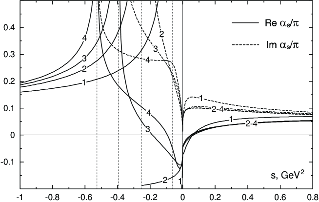
Figure 1: Real and imaginary parts of $\alpha_{\overline{\rm MS}}(s)/\pi$ as exact numerical solution of RG equation (9) on real axes for different number of loops. The initial condition is chosen $\alpha_{s}=0.355$ at $s=-m_{\tau}^{2}$, $N_{f}=3$. Vertical dotted lines display the position of the unphysical singularity at $s=-Q_{0}^{2}$ for each approximation ($4\to 1$ from left to right).

It is well known, that in the 1-loop approximation of $\beta$ function the coupling $a(Q^{2})$ has an infrared pole at some $Q^{2}=Q^{2}_{0}$ (in some conventions coinciding with $\Lambda^{2}$). In the $n$-loop approximation ($n>1$) instead of pole a branch cut appears with a singularity $\sim(1-Q^{2}/Q^{2}_{0})^{-1/n}$. The position of the singularity is given by

$$\ln{Q_{0}^{2}\over\mu^{2}}\,=\,-\,\int_{a(\mu^{2})}^{\infty}{da\over\beta(a)}$$ (12)

Near the singularity the last term in the expansion of $\beta(a)$ (9) dominates and gives the aforementioned behavior. To illustrate the behavior of the running coupling constant, we plotted real and imaginary part of $\alpha_{s}/\pi$ for $n=1,2,3,4$-loop $\beta$-function in Fig 1. It demonstrates, that for real positive $s$ the difference between various approximations is almost unnoticable beyond 2-nd loop and the expansion in inverse $|\ln{(s/\Lambda^{2})}-i\pi|$ works well. At the same time the behavior in the unphysical cut strongly depends on the number of loops and cannot be described by some simple approximation. Only at $s<1\,{\rm GeV}^{2}$ 2–4 loop calculations more or less coincide.

Let us turn now to OPE terms in (7). The contribution of the operators up to dimension 8 have been computed theoretically:

$$\sum_{n\geq 2}{\left<O_{2n}\right>\over(-s)^{n}}\left(1+c_{n}{\alpha_{s}\over\pi}\right) = {\alpha_{s}\over 6\pi\,Q^{4}}\left<G_{\mu\nu}^{a}G_{\mu\nu}^{a}\right>\left(1+{7\over 6}{\alpha_{s}\over\pi}\right)$$ (13)

$$+ {128\over 81\,Q^{6}}\,\pi\alpha_{s}\left<\bar{q}q\right>^{2}\left[1+\left({29\over 24}+{17\over 18}\ln{Q^{2}\over\mu^{2}}\right){\alpha_{s}\over\pi}\right]+{\left<O_{8}\right>\over Q^{8}}$$

The contribution of $D=2$ operator due to nonzero quark masses $m_{u,d}$ is negligible and omitted here. We have also neglected the $D=4$ quark condensate $2(m_{u}+m_{d})\left<\bar{q}q\right>$ which is an order of magnitude less than the gluonic condensate. The coefficients in front of $D=4,6$ operators have been computed in [21], hereafter cited as SVZ. The $\alpha_{s}$-correction to the $D=4$ operator were found in [22]; $\alpha_{s}$-corrections to $D=6$ operator were calculated [23]; ambiguities among them were also discussed there.

Few comments about the operator $O_{6}$ are in order. In nonfactorized form without $\alpha_{s}$-corrections it looks as follows [21]:

$$\left<O_{6}\right> = -2\pi\alpha_{s}\Biggl{<}(\bar{u}\gamma_{\mu}\lambda^{a}d)(\bar{d}\gamma_{\mu}\lambda^{a}u)+(\bar{u}\gamma_{5}\gamma_{\mu}\lambda^{a}d)(\bar{d}\gamma_{5}\gamma_{\mu}\lambda^{a}u)$$ (14)

$$\hskip 36.98857pt+\,{2\over 9}(\bar{u}\gamma_{\mu}\lambda^{a}u+\bar{d}\gamma_{\mu}\lambda^{a}d)\sum_{u,d,s}(\bar{q}\gamma_{\mu}\lambda^{a}q)\Biggr{>}$$

After factorization three terms in (14) give the following contributions:

$$\left<O_{6}\right>\,=\,4\pi\alpha_{s}\left<\bar{q}q\right>^{2}\left(1-{1\over N_{c}^{2}}\right)\left(1-1+{4\over 9}\right)$$ (15)

where $N_{c}$ is the number of colors. SVZ assumed that the accuracy of the factorization procedure is of order $N_{c}^{-2}\sim 10\%$ in case of $V$-correlator, where the coefficient in the second brackets in (15) is equal to $-7/9$. Remind that in $V-A$ correlator the first term has opposite sign and the third term is absent, so the accuracy of the factorized operator $O_{6}^{V-A}$ is at least not worse, than in $V$ case. On the other hand in the $V+A$ correlator two comparatively large terms cancel each other under the factorization assumption in (15). Consequently the accuracy of the formula (15) for the operator $O_{6}$ is less, perhaps $20-30\%$. Large $\alpha_{s}$-corrections to all independent $D=6$ operators [23] can only increase the errors.

The numerical value of $D=6$ operator can be estimated, for instance, with help of our previous analysis of $V-A$ sum rules [5]:

$$\bigl{<}O_{6}^{V-A}\bigr{>}\,=\,-\,{64\over 9}\,\pi\alpha_{s}\left<\bar{q}q\right>^{2}\times 1.3\,=\,-\,(6.8\pm 2.1)\times 10^{-3}\,{\rm GeV}^{6}$$ (16)

The coefficient $1.3$ stands for the $\alpha_{s}$-corrections. We find:

$$\left<O_{6}\right>\,=\,(1.3\pm 0.5)\times 10^{-3}\,{\rm GeV}^{6}\;,$$ (17)

The dimension 8 operators come from many different diagrams, which can be labeled by the number of quarks in vacuum. The purely gluonic condensates are suppressed by the loop factor $\sim\alpha_{s}/\pi$ and are neglected on this ground. The 4-quark operators, computed in [24, 25] and [5], vanish in the sum $V+A$ after factorization. The uncertainty of this cancellation can be estimated as $\sim 10\%$ of $O_{8}^{V-A}$, which is about $10^{-3}\,{\rm GeV}^{8}$. The 2-quark operators have the same sign in $V$ and $A$ correlators. They have been computed in [26] (we have performed the calculation independently to confirm this result) and can be written in the following form:

$$\bigl{<}O_{8}^{(2)}\bigr{>} = {2\over 9}\,\Biggl{<}\,2i\,\bar{u}\gamma^{\alpha}\{G^{2}_{(\alpha\beta)},D^{\beta}\}u\,-\,\bar{u}\gamma^{\alpha}\gamma^{5}\{(\tilde{G}G)_{\alpha\beta},D^{\beta}\}u\,+\,{i\over 4}\,\bar{u}\gamma^{\gamma}\!\left[G^{\alpha\beta},(D_{\gamma}G_{\alpha\beta})\right]\!u$$ (18)

$$\left.\,+\,{1\over 2}\,\bar{u}(D^{2}\hat{J})u\,-\,i\bar{u}\gamma^{\alpha}\!\left[G_{\alpha\beta},J^{\beta}\right]\!u\,\right>+\,(u\to d)$$

where $J_{\mu}=D_{\nu}G_{\mu\nu}=\pi\alpha_{s}\lambda^{a}\sum_{q}(\bar{q}\gamma_{\mu}\lambda^{a}q)$. The last two terms can be factorized and brought to the form $\pi\alpha_{s}\!\left<\bar{q}q\right>\!\bigl{<}\bar{q}\hat{G}q\bigr{>}$. However the leading in the number of colors $N_{c}^{0}$ terms cancel each other and only the terms $\sim N_{c}^{-2}$ are left. It has been shown in [5], that the factorization of $D=8$ operators is not unambiguous at this level of accuracy. Taking the value of the operator $\bigl{<}\bar{q}\hat{G}q\bigr{>}$ from [27, 5], we may estimate the upper limit of the operator (18) as $|\bigl{<}O_{8}^{(2)}\bigr{>}|<10^{-4}\,{\rm GeV}^{8}$, which is tiny. So, for the upper limit of the total $D=8$ operator we shall use the estimation $|\bigl{<}O_{8}\bigr{>}|<10^{-3}\,{\rm GeV}^{8}$.

It is worth mentioned, that the $D=6,8$ operators in $V+A$ polarization function are much smaller, than in $V$ or $A$ separately.

We are now in position to calculate $\alpha_{s}(m_{\tau}^{2})$ from the experiment. We take the most recent data on the total hadronic decay ratio $R_{\tau}$ [7] and the ratio of decays with odd number of strange mesons $\tau^{-}\to X(S=-1)\nu_{\tau}$ [28, 29]:

$$R_{\tau}\,=\,3.636\pm 0.021\;,\qquad R_{\tau,S}\,=\,0.161\pm 0.007$$ (19)

In our analysis we subtract $R_{\tau,S}$ to avoid the interference with additional parameters, in particular the mass of $s$-quark. One obtains

$$R_{\tau,V+A}=3|V_{ud}|^{2}S_{EW}\left(\,1\,+\,\delta_{EW}^{\prime}\,+\,\delta^{(0)}\,+\,\delta^{(6)}_{V+A}\,\right)+\Delta R^{(0)}\,=\,3.475\pm 0.022$$ (20)

where $\Delta R^{(0)}_{\tau}$ is given by (5). We use conventional in $\tau$-literature notations of fractional corrections $\delta$. The electromagnetic correction is $\delta_{EW}^{\prime}={5\over 12\pi}\alpha_{em}(m_{\tau}^{2})=0.001$ [30], the $D=6$ operator correction $\delta^{(6)}_{V+A}=-(5\pm 2)\times 10^{-3}$ as follows from our analysis, in agreement with the estimation obtained in [12]. From (20) we separate out the perturbative correction:

$$1\,+\,\delta^{(0)}\,=\,1.206\pm 0.010$$ (21)

All errors in here are added in quadratures (perhaps, such procedure underestimates the total error, may be by a factor 2).

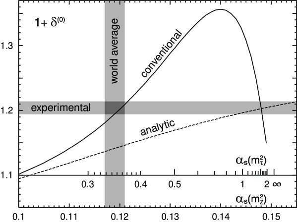
Figure 2: Perturbative fractional correction $\delta^{(0)}$ versus $\alpha_{s}(m_{\tau}^{2})$ and $\alpha_{s}(m_{Z}^{2})$ in conventional and analytical approach in 3-loop approximation. In the width of the experimental strip the theoretical uncertainty of the operator $\left<O_{6}\right>$ is included.

The calculation of $\alpha_{s}(m_{\tau}^{2})$ corresponding to $\delta^{(0)}$ were performed according to the method described above. The dependence of $1+\delta^{(0)}$ on $\alpha_{s}(m_{\tau}^{2})$ (and on $\alpha(M_{Z}^{2})$, to compare with other data) for 3-loop $\beta$-function and 3-loop Adler function is shown of Fig 2. It follows from Fig 2:

$$\alpha_{s}(m_{\tau}^{2})\,=\,0.355\pm 0.025$$ (22)

The estimation of the error in (22) was done with care. Because of asymptotic character of perturbative series (8) and (9) the higher loop contribution could be as large as the contribution of the last terms, namely $K_{3}a^{3}$ and $\beta_{2}a^{4}$. They result to uncertainty $0.015-0.20$ in $\alpha_{s}(m_{\tau}^{2})$, depending on its central value. Taking into account the uncertainty (21) in $\delta^{(0)}$, we obtain the error in (22). Furthermore, we have performed 2 and 4-loop calculation of $\alpha_{s}(m_{\tau}^{2})$. The unknown 4-loop coefficient in Adler function (8) was taken equal to $K_{4}=50$ (cf. its estimations [31]). For each given $\delta^{(0)}$ the 4-loop $\alpha_{s}(m_{\tau}^{2})$ is by $0.005$ lower than 3-loop value, while 2-loop $\alpha_{s}(m_{\tau}^{2})$ is by $0.02$ higher. These results are within the error range (22). If some nonperturbative terms beyond OPE exist (e.g. instantons), they would also contribute to the error in (22). In section 4 it will be shown, that the value $\alpha_{s}(m_{\tau}^{2})$ close to the lower limit of (22) satisfies sum rules at low $Q^{2}$ much better.

3 $\alpha_{s}(m_{\tau}^{2})$ and analytical QCD

Shirkov and Solovtsov [32] forwarded the idea of analytical QCD. According to it the coupling constant $\alpha_{s}(Q^{2})$ is calculated by renormalization group in the space-like region $Q^{2}>0$. Then, by analytical continuation to $s=-Q^{2}>0$, $\alpha_{s}(s)$ was found, in particular its imaginary part ${\rm Im}\,\alpha_{s}(s)$ on the right semiaxes. It was assumed, that $\alpha_{s}(s)$ is an analytical function in the complex $s$-plane with a cut along the right semiaxes $0\leq s<\infty$. The analytical $\alpha_{s}(s)_{\rm an}$ is then defined in the whole complex $s$-plane by dispersion relation:

$$\alpha_{s}(s)_{\rm an}\,=\,{1\over\pi}\,\int_{0}^{\infty}{{\rm Im}\,\alpha_{s}(s^{\prime})\over s-s^{\prime}}\,ds^{\prime}$$ (23)

Since the lower limit in this integral is put to zero, $\alpha_{s}(s)_{\rm an}$ indeed has no unphysical singularities (poles, cuts etc) at $Q^{2}>0$. The idea of analytical QCD has been developed in many papers, see e.g. [33] and for review [34]. In particular the calculations of $\alpha_{s}(m_{\tau}^{2})_{\rm an}$ from $\tau$-decay data were performed within the framework of analytical QCD in [35].

A related approach was suggested by two of us (B.G. and B.I.) in [36]. We started from well-known theorem, that the polarization operator for $e^{+}e^{-}$ annihilation $\Pi(s)$ is an analytical function of $s$ in complex $s$-plane with a cut along positive semiaxes and assumed that these analytical properties take place separately for perturbative and nonperturbative parts of $\Pi(s)$. In the first order of $\alpha_{s}$ this hypothesis is equivalent to analytical QCD while in higher orders it may be more general.

Let us calculate $\alpha_{s}(m_{\tau}^{2})_{\rm an}$ in the framework of analytical QCD from the same experimental data, i.e. $\delta^{(0)}$ given by (21). The only (but important) difference from the previous calculation is the following. The coupling $\alpha_{s}(s)_{\rm an}$ is an analytical function of $s$ with a cut from $s=0$ to $s=\infty$. Consequently the contour integral in (6) is now equal to the original integral (4) with ${\rm Im}\,\Pi(s)$ over real positive axes. In the previous calculation, if such transformation is performed, the integral would run from $s=-Q_{0}^{2}$ to $m_{\tau}^{2}$. Qualitatively it leads to much smaller $R_{\tau}$ in analytical QCD than in conventional approach with the same $\alpha_{s}(m_{\tau}^{2})$, or vice versa, the same $R_{\tau}$ corresponds to much larger $\alpha_{s}(s)_{\rm an}$. Direct numerical calculation confirms this expectation. The dependence of $1+\delta^{(0)}$ versus $\alpha_{s}(s)_{\rm an}$ is also displayed in Fig 2. It is seen, that in order to get experimental value of $\delta^{(0)}$ in analytical QCD one should take $\alpha_{s}(m_{\tau}^{2})_{\rm an}\approx 1.5-2.0$, which corresponds to $\alpha_{s}(m_{Z}^{2})\approx 0.15$ in strong contradiction with the world average $\alpha_{s}(m_{Z}^{2})=0.119\pm 0.002$ [7]. (The previous calculation of $\tau$-decay [35], performed with less certainty, demonstrated the same trend: in particular $\Lambda^{(3)}=700-900\,{\rm MeV}$, much larger, than in standard calculations.)

It the recent paper [37] an attempt was made to save the analytical QCD in case of vector polarization operator and to obtain the agreement with ALEPH data on vector Adler $D$-function by assuming large quark masses $m_{u}=m_{d}=250\,{\rm MeV}$ and some form of Coulomb-like quark-antiquark interaction. This hypothesis, however, is in strong contradiction with all results following from well established partial conservation of axial current (PCAC) and chiral theory. For example, Gell-Mann-Oakes-Renner relation and $K/\pi$ mass ratios would be violated by an order of magnitude, Goldberg-Treitman relation cannot be proved etc. Also many sum rules for $V-A$ polarization operator would disagree with the data.

Therefore we come to the conclusion, that analytical QCD in any form, [32] or [36] is in strong contradiction with experiment and must be abandoned.

4 Check of QCD at low $Q^{2}$ for $V+A$ correlators by using the sum rules

Let us turn now to study of the $V+A$ correlator in the domain of low $Q^{2}$, where the OPE terms play much more essential role, than in the determination of $R_{\tau}$. A general remark is in order here. As was mentioned in [38] and stressed recently by Shifman [39], the condensates cannot be defined in rigorous way, because there is some arbitrariness in the separation of their contributions from perturbative part. Usually [38, 39] they are defined by introduction of some normalization point $\mu^{2}$ with the magnitude of few $\Lambda^{2}$. The integration over momenta in the domain below $\mu^{2}$ is addressed to condensates, above $\mu^{2}$ — to perturbation theory. In such formulation the condensates are $\mu$-dependent $\left<O_{D}\right>=\left<O_{D}\right>_{\mu}$ and, strictly speaking, they also depend on the way how the infrared cut-off $\mu^{2}$ is introduced. The problem becomes more severe when the perturbative expansion is performed up to higher order terms and the calculation pretends on high precision. Mention, that this remark does not refer to chirality violating condensates, because perturbative terms do not contribute to chirality violating structures. For this reason, in principle, chirality violating condensates, e.g. $\bigl{<}0|\bar{q}q|0\bigr{>}$, can be determined with higher precission, than chirality conserving ones. Here we use the definition of condensates, which can be called $n$-loop condensates. As was formulated in Section 2, we treat the renormalization group equation (9) and the equation for polarization operator (10) in $n$-loop approximation as exact ones; the expansion in inverse logarithms is not performed. Specific values of condensates are referred to such procedure. Of course, their numerical values depend on the accounted number of loops; that is why the condensates, defined in this way, are called $n$-loop condensates.

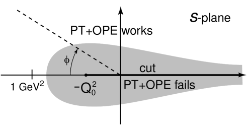
Figure 3: Region of validity of the perturbation theory (PT) and operator product expansion (OPE)

Consider the polarization operator $\Pi=\Pi_{V+A}^{(1)}+\Pi_{A}^{(0)}$, defined in (1) and its imaginary part

$$\omega(s)\,=\,v_{1}(s)\,+\,a_{1}(s)\,+\,a_{0}(s)\,=\,2\pi\,{\rm Im}\,\Pi(s+i0)$$ (24)

In parton model $\omega(s)\to 1$ at $s\to\infty$. Any sum rule can be written in the following form:

$$\int_{0}^{s_{0}}f(s)\,\omega_{\rm exp}(s)\,ds\,=\,i\pi\oint f(s)\,\Pi_{\rm theor}(s)\,ds$$ (25)

where $f(s)$ is some analytical in the integration region function. In what follows we use $\omega_{\rm exp}(s)$, obtained from $\tau$-decay invariant mass spectra published in [1] for $0<s<m_{\tau}^{2}$ with step $ds=0.05\,{\rm GeV}^{2}$. The experimental error of the integral (25) is computed as the double integral with the covariance matrix $\overline{\omega(s)\omega(s^{\prime})}-\overline{\omega}(s)\overline{\omega}(s^{\prime})$, which also can be obtained from the data available in [1]. In the theoretical integral in (25) the contour goes from $s_{0}+i0$ to $s_{0}-i0$ counterclockwise around all poles and cuts of theoretical correlator $\Pi(s)$, see Fig 3. Because of Cauchy theorem the unphysical cut must be inside the integration contour.

The choice of the function $f(s)$ in (25) is actually a matter of taste. At first let us consider usual Borel transformation:

$$B_{\rm exp}(M^{2})\,=\,\int_{0}^{m_{\tau}^{2}}e^{-s/M^{2}}\omega_{\rm exp}(s)\,{ds\over M^{2}}\,=\,B_{\rm pt}(M^{2})\,+\,2\pi^{2}\sum_{n}{\bigl{<}O_{2n}\bigr{>}\over(n-1)!\,M^{2n}}$$ (26)

We separated out the purely perturbative contribution $B_{\rm pt}$, which is computed numerically according to (25) and (8–10). Remind that Borel transformation improves the convergence of OPE series because of the factors $1/(n-1)!$ in front of operators and suppresses the contribution of high-energy tail, where the experimental error is large. But it does not suppress the unphysical perturbative cut, the main source of the error in this approach, even increase it since $e^{-s/M^{2}}>1$ for $s<0$. So the perturbative part $B_{\rm pt}(M^{2})$ can be reliably calculated only for $M^{2}\approx 0.8-1\,{\rm GeV}^{2}$ and higher; below this value the influence of the unphysical cut is out of control.

Both $B_{\rm exp}$ and $B_{\rm pt}$ in 3-loop approximation for $\alpha_{s}(m_{\tau}^{2})=0.355$ and $0.330$ are shown in Fig 4. The shaded areas display the theoretical error. They are taken equal to the contribution of the last term in the perturbative Adler function expansion $K_{3}a^{3}$ (8). We have also performed the calculation with 4-loop $\beta$-function and $K_{4}=50\pm 50$, but the result is very close to the 3-loop one, since positive contribution of the term $K_{4}a^{4}$ compensates small decrease in the coupling $a$. Since this result is observed by us in many other sum rules, we shall not give the 4-loop calculations later on and estimate the theoretical error for any given $a(m_{\tau}^{2})$ as the contribution of $K_{3}a^{3}$.

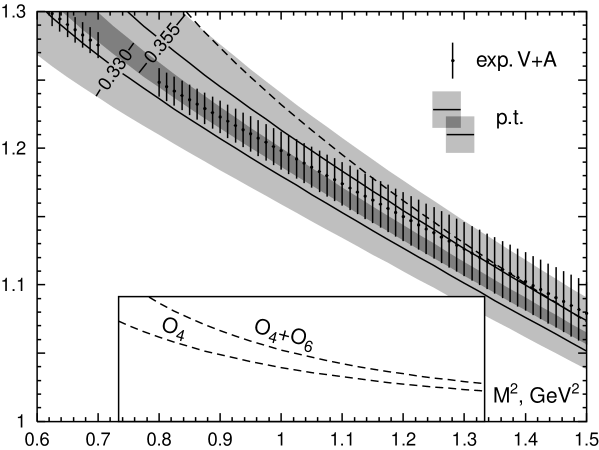
Figure 4: Borel transformation (26) $B_{\rm exp}(M^{2})$ and $B_{\rm pt}(M^{2})$ for $\alpha_{s}(m_{\tau}^{2})=0.355$ and $0.330$. The dashed line displays the OPE contribution added to the $0.330$-perturbative curve. The contribution of the operators $D=4$ (standard SVZ value) and $D=6$ (central value of (17)) with respect to 1 are shown separately in the box.

As follows from the analysis in Section 2, for $M^{2}>1\,{\rm GeV}^{2}$ the contribution of $D=6,8$ operators to the Borel transform (26) is small in $V+A$ channel, while the contribution of the $D=4$ condensate must be positive (we assume $\alpha_{s}$-corrections included in the operators $\bigl{<}O_{2n}\bigr{>}$ in (26) and later). So the theoretical curve must go below experimental one. The result shown in Fig 4 is in favor of lower value of the coupling constant $\alpha_{s}(m_{\tau}^{2})=0.33$. Literally the theoretical curve (perturbative at $\alpha_{s}(m_{\tau}^{2})=0.33$ plus the contribution of $O_{4}$ and $O_{6}$ operators) agrees with experiment starting from $M^{2}=1.1\,{\rm GeV}^{2}$. If the uncertainties in perturbative contributions are taken into account (shaded area in Fig 4) the agreement may start earlier, at $M^{2}=1\,{\rm GeV}^{2}$.

The Borel transformation on Fig 4 includes the contributions of different operators. Although it is difficult to separate the perturbative part from the OPE one, the contributions of different operators can be separated from each other. One way is to differentiate the Borel transformation by $M^{2}$. This however leads to the certain loss in the accuracy of the experimental integral, since the growing power term $\sim s^{n}$ appears in the integral. So we apply the method used in [5] for $V-A$ sum rules, namely the Borel transformation in complex $M^{2}$ plane.

Let us consider the Borel transform $B(M^{2})$ (26) at some complex $M^{2}=M_{0}^{2}e^{i\phi}$, $0<\phi<\pi/2$. If the phase $\phi$ is taken close to $\pi/2$ then the contribution of the high-energy tail becomes high. So we restrict ourselves by the values $\phi\leq\pi/4$ for the exponent to be decreasing enough. The real part of the Borel transform at $\phi=\pi/6$ does not contain the $D=6$ operator:

$${\rm Re}\,B_{\rm exp}(M^{2}e^{i\pi/6})\,=\,{\rm Re}\,B_{\rm pt}(M^{2}e^{i\pi/6})\,+\,\pi^{2}\,{\bigl{<}O_{4}\bigr{>}\over M^{4}}$$ (27)

The contribution of $\bigl{<}O_{8}\bigr{>}$ is less than $0.5\%$ to the perturbative term and neglected here. The results are shown in Fig 5a. Again it is still difficult to accommodate positive value of the gluonic condensate to the coupling $\alpha_{s}(m_{\tau}^{2})=0.355$ and higher. If we accept the lower value of $\alpha_{s}(m_{\tau}^{2})$, we get the following restriction on the value of the gluonic condensate:

$$\left<{\alpha_{s}\over\pi}\,G_{\mu\nu}^{a}G_{\mu\nu}^{a}\right>\,=\,0.006\pm 0.012\,{\rm GeV}^{4}\;,\qquad\alpha_{s}(m_{\tau}^{2})=0.330\quad{\rm and}\quad M^{2}>0.8\,{\rm GeV}^{2}$$ (28)

The theoretical and experimental errors are added together in (28).

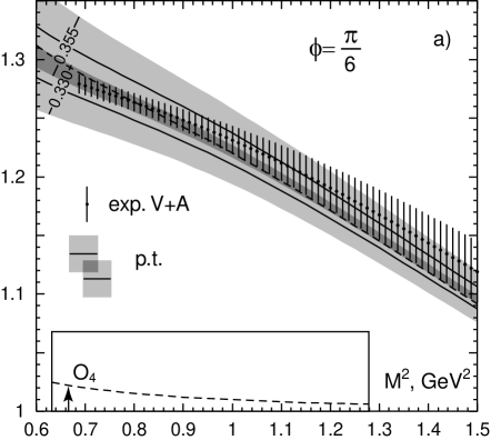
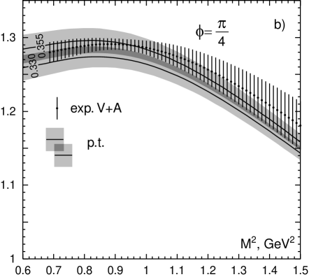
Figure 5: Real part of the Borel transform (26) along the rays at the angles $\phi=\pi/6$ and $\pi/4$ to the real axes. The dash line corresponds to the gluonic condensate given by the central value of (28).

The real part of the Borel transform at $\phi=\pi/4$ does not contain the $D=4$ operator:

$${\rm Re}\,B_{\rm exp}(M^{2}e^{i\pi/4})\,=\,{\rm Re}\,B_{\rm pt}(M^{2}e^{i\pi/4})\,-\,\pi^{2}\,{\bigl{<}O_{6}\bigr{>}\over\sqrt{2}M^{6}}$$ (29)

The results are shown in Fig 5b. The perturbative curve at $\alpha_{s}=0.330$ is below the data. If we would take this curve as an exact one, without accounting the perturbative errors, then from (29) we would conclude, that $\left<O_{6}\right><0$, which in some contradiction with (13, 17). However the account for the perturbative errors makes the situation different, but uncertain. Since the value of the $\left<O_{6}\right>$ contribution to (29) is very small

$$\pi^{2}{\bigl{<}O_{6}\bigr{>}\over\sqrt{2}M^{6}}=(0.9\pm 0.4)\times 10^{-2}\,{{\rm GeV}^{6}\over M^{6}}$$ (30)

then by accounting the perturbative errors it is possible to satisfy the sum rule (29) at positive $\left<O_{6}\right>$ starting from $M^{2}>0.8\,{\rm GeV}^{2}$. (In the narrow region near $M^{2}=0.9\,{\rm GeV}^{2}$ the theoretical curve goes out of the data on $1.5-2$ experimental error, but we do not consider this as a serious contradiction.) Unfortunately no definite conclusion about the value of $O_{6}$ can be done from the Fig 5b. The only statement is that its value cannot exceed (17) and probably is on the lower border of error.

5 Correlator of vector currents

Previously we considered the $V+A$ correlators where the power corrections are small. Instead one could take pure vector current, (vector spectral function was published by ALEPH in [40]). This doesn’t give us any new information with the $\tau$-decay data, since $V-A$ correlators have already been analyzed in [5]. Moreover the accuracy of the vector current spectral function is less, than $V+A$, since both currents are mixed in some channels with $K$-mesons and the number of events is twice less.

However the analysis of the vector current correlator is important since it can also be performed with the experimental data on $e^{+}e^{-}$ annihilation. The imaginary part of the electromagnetic current correlator, measured here, is related to the charged current correlator (1) by the isotopic symmetry. The statistical error in $e^{+}e^{-}$ experiments is less than in $\tau$-decays because of significantly larger number of events. So it would be interesting to perform similar analysis with $e^{+}e^{-}$ data, which is a matter for separate research.

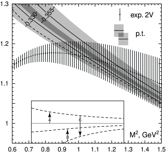
Figure 6: Borel transformation for vector currents.

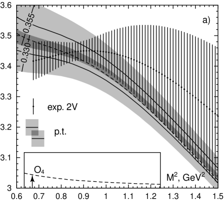
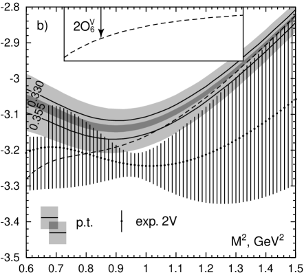
Figure 7: The sum rules (31) (a) and (32) (b) for vector currents.

At first we consider usual Borel transformation for vector current correlator, since it was originally applied in [4] for the sum rule analysis. It is defined as (26) with the experimental spectral function $\omega_{\rm exp}=2v_{1}$ instead of $v_{1}+a_{1}+a_{0}$ (the normalization is $v_{1}(s)\to 1/2$ at $s\to\infty$ in parton model). Respectively, in the r.h.s. one should take the vector operators $2O^{V}=O^{V+A}+O^{V-A}$, all $O^{V-A}$ with $D\leq 8$ can be found in [5]. Numerical results are shown in Fig 6. The perturbative theoretical curves are the same as in Fig 4 with $V+A$ correlator. The dashed lines display the contributions of the gluonic condensate given by (28), $2O_{6}^{V}=-5.5\times 10^{-3}\,{\rm GeV}^{6}$ and $2O_{8}^{V}=O_{8}^{V-A}=7\times 10^{-3}\,{\rm GeV}^{8}$ added to the $0.330$-perturbative curve. The contribution of each condensate is shown in the box below. Notice, that for such condensate values the total OPE contribution is small, since positive $O_{4}$ and $O_{8}$ compensate negative $O_{6}$. The agreement is observed for $M^{2}>0.8\,{\rm GeV}^{2}$.

Now we apply the method of Borel transformation along the rays to the vector polarization operator to separate the contribution of different operators from each other. The $D=8$ operator is important here, so we shall separate $O_{4,6}$ from $O_{8}$.

Borel transformation at low $M^{2}$ exponentially suppresses the contribution of large $s$ domain, where the experimental error is high. Besides of this we may use the oscillating behavior of the complex exponent to further suppress the high-error points near $s=m_{\tau}^{2}$. This would allow us to go to higher $M^{2}$. Here the real part of $B(M^{2})$ has obvious advantage since the function $\cos{(\phi+{s\over M^{2}}\cos{\phi})}$ has zero at $s=m_{\tau}^{2}$ and $\phi\sim\pi/4$ already at $M^{2}\approx 1\,{\rm GeV}^{2}$, while the largest (in $M^{2}$) zero of $\sin{(\phi+{s\over M^{2}}\cos{\phi})}$ in imaginary part is twice lower. So let us take three different angles, say, $\phi=0,\pi/6,\pi/4$. Solving the system of linear equations, we get:

$${\rm Re}\,\left[\,{B(0)\over 2-\sqrt{2}}\,-\,\sqrt{2}\,B(\pi/6)\,+\,{B(\pi/4)\over\sqrt{2}-1}\,\right] = {\rm p.t.}\,+\,2\pi^{2}\,{O_{4}\over M^{4}}$$ (31)

$${\rm Re}\,{-\,B(0)\,+\,2\,B(\pi/6)\,-\,2\,B(\pi/4)\over\sqrt{2}-1} = {\rm p.t.}\,+\,2\pi^{2}\,{O_{6}\over 2M^{6}}$$ (32)

For brevity we write here $B(\phi)$ instead of $B_{\rm exp}(M^{2}e^{i\phi})$, ”p.t.” stands for perturbative contribution. The results for the equations (31, 32) are shown in Figs 7a,b respectively.

Fig 7a demonstrates, that the vector sum rule is satisfied at $\alpha_{s}(m_{\tau}^{2})=0.330$ and gluonic condensate (28) (although higher values of gluonic condensate, e.g. SVZ value still do not contradict the data). Fig 7b shows, that the $O_{6}^{V}$ contribution works in right direction: its addition to 0.330-perturbative curve shrinks the disagreement between the theory and experiment. However, some discrepancy (about 0.04, i.e. $0.1\%$ in the worst case) still persist. It may be addressed either to the uncertainty in $\alpha_{s}(m_{\tau}^{2})$ — a slightly higher value would be desirable, or to the underestimation of $O_{6}^{V}$ (in absolute value: $O_{6}^{V}$ is negative) by $20-30\%$, or both. Remind, that the numerical values of condensates depend on the way, how the infrared region is treated ($O_{6}$ is chirality conserving). We are considering here 3-loop condensates, defined in Sec. 4. The $O_{6}^{V}$ value was taken equal to $7/18$ of $O_{6}^{V-A}$, obtained from $V-A$ data analysis [5], where perturbative terms are absent, and some difference is not excluded.

6 The check for renormalon-type terms

In the asymptotic perturbative series a special part of terms — renormalons (infrared and ultraviolet) is often separated and the summation of them is performed (for a recent review see [41]). In such sum the term appears proportional to $1/Q^{2}$ at large $Q^{2}$ and looking as a contribution of $D=2$ operator. (In OPE the $D=2$ operator is proportional to $m_{q}^{2}$ and is very small.) Renormalons conserve chirality and may contribute to $V+A$ but not to $V-A$. Unfortunately, the coefficient in front of the $1/Q^{2}$ term of the renormalon origin cannot be calculated reliably. (In [42] it was claimed, that the renormalons are totally absent in the perturbative series asymptotics and therefore this coefficient is zero.) In recent paper [43] the hypothesis was suggested, that infrared renormalons result in substitution

$${\alpha_{s}\over\pi}\,\to\,{\alpha_{s}\over\pi}\left(\,1\,-\,1.05\,{\lambda^{2}\over Q^{2}}\right)$$ (33)

in the first $\alpha_{s}$ correction to polarization operator or Adler function (the $Q^{2}$-dependence of $\alpha_{s}$ was not accounted in [43]). In (33) $\lambda^{2}$ is tachionic gluon mass, $\lambda^{2}<0$ and for its value the estimation was found:

$$-\,\lambda^{2}\,=\,(0.2-0.5)\,{\rm GeV}^{2}$$ (34)

The authors of [43] could not discriminate even the highest value $\lambda^{2}=-0.5\,{\rm GeV}^{2}$.

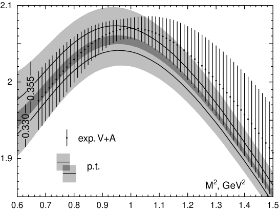
Figure 8: Sum rule (35) with $O_{2}$ but without $O_{4,6}$

Let us try to find the restriction on $O_{2}$ operator from the sum rule for $V+A$ correlator in the complex $q^{2}$-plane from ALEPH data. (We call it for brevity $O_{2}$, although it is not the $D=2$ operator which stands in OPE.) As we did in previous section, for this purpose we take the real part of the Borel transform (26) $B(M^{2}e^{i\phi})$ at the angles $\phi=0,\pi/6,\pi/4$ and separate the operator $O_{2}$ from $O_{4,6}$:

$${\rm Re}\,{B(0)\,-\,2\,B(\pi/6)\,+\,\sqrt{2}\,B(\pi/4)\over 2-\sqrt{3}}\,=\,{\rm p.t.}\,+\,2\pi^{2}\,{O_{2}\over M^{2}}$$ (35)

The experimental and perturbative parts of this combination are plotted in Fig 8.

The sum rule (35) shown in Fig 8 gives the following value of the dimension 2 operator:

$$O_{2}\,=\,(1.0\pm 1.5)\times 10^{-3}\,{\rm GeV}^{2}\;,\qquad\alpha_{s}(m_{\tau}^{2})=0.33$$ (36)

We got this estimation at $M^{2}=1\,{\rm GeV}^{2}$, where experimental error is minimal. In the model of [43]

$$O_{2}\,=\,-1.05\,{\alpha_{s}\over\pi}\,\lambda^{2}$$ (37)

At $\alpha_{s}(1\,{\rm GeV}^{2})/\pi=0.18$, corresponding to $\alpha_{s}(m_{\tau}^{2})=0.33$, there follows the restriction from (36):

$$-\,\lambda^{2}\,=\,(5\pm 8)\times 10^{-2}\,{\rm GeV}^{2}$$ (38)

which is few times smaller than even the lower limit in (34). Notice, that similar restrictions on the value of $D=2$ operator have been obtained in [44] from other sum rules.

7 Instanton corrections

Some nonperturbative features of QCD may be described in so called instanton gas model (see [45] for extensive review and the collection of related papers in [46]). Namely, one computes the correlators in the $SU(2)$-instanton field embedded in the $SU(3)$ color group. In particular, the 2-point correlator of the vector currents has been computed long ago [47]. Apart from usual tree-level correlator $\sim\ln{Q^{2}}$ it has a correction which depends on the instanton position and radius $\rho$. In the instanton gas model these parameters are integrated out. The radius is averaged over some concentration $n(\rho)$, for which one or another model is used. Concerning the 2-point correlator of charged axial currents, the only difference from the vector case is that the term with 0-modes must be taken with opposite sign. In coordinate representation the answer can be expressed in terms of elementary functions, see [47]. An attempt to compare the instanton correlators with ALEPH data in coordinate space has been undertaken in [48].

We shall work in momentum space. Here the instanton correction to the spin-$J$ parts $\Pi^{(J)}$ of the correlator (1) can be written in the following form:

$$\Pi^{(1)}_{V,\,{\rm inst}}(q^{2}) = \int_{0}^{\infty}\!d\rho\,n(\rho)\,\left[\,-\,{4\over 3q^{4}}\,+\,\sqrt{\pi}\rho^{4}G^{30}_{13}\left(-\rho^{2}q^{2}\left|{1/2\atop 0,0,-2}\right.\right)\right]$$

$$\Pi^{(0)}_{A,\,{\rm inst}}(q^{2}) = \int_{0}^{\infty}\!d\rho\,n(\rho)\,\left[\,-\,{4\over q^{4}}\,-\,{4\rho^{2}\over q^{2}}\,K_{1}^{2}\!\left(\rho\sqrt{-q^{2}}\right)\right]$$

$$\Pi^{(1)}_{A,\,{\rm inst}}(q^{2}) = \Pi^{(1)}_{V,\,{\rm inst}}(q^{2})-\Pi^{(0)}_{A,\,{\rm inst}}(q^{2})\;,\qquad\Pi^{(0)}_{V,\,{\rm inst}}(q^{2})\,=\,0$$ (39)

Here $K_{1}$ is modified Bessel function, $G_{mn}^{\,p\,q}(z|\ldots)$ is Meijer function. Definitions, properties and approximations of Meijer functions can be found, for instance, in [49]. In particular the function in (39) can be written as the following series:

$$\sqrt{\pi}G^{30}_{13}\left(z\left|{1/2\atop 0,0,-2}\right.\right) = {4\over 3z^{2}}\,-\,{2\over z}\,+\,{1\over 2\sqrt{\pi}}\,\sum_{k=0}^{\infty}\,z^{k}{\Gamma(k+1/2)\over\Gamma^{2}(k+1)\,\Gamma(k+3)}\times$$ (40)

$$\times\Bigl{\{}\,\left[\,\ln{z}\,+\,\psi(k+1/2)\,-\,2\,\psi(k+1)\,-\,\psi(k+3)\,\right]^{2}$$

$$+\,\psi^{\prime}(k+1/2)\,-\,2\,\psi^{\prime}(k+1)\,-\,\psi^{\prime}(k+3)\,\Bigr{\}}$$

where $\psi(z)=\Gamma^{\prime}(z)/\Gamma(z)$. For large $|z|$ one can obtain its approximation by the saddle-point method:

$$G^{30}_{13}\left(z\left|{1/2\atop 0,0,-2}\right.\right)\approx\sqrt{\pi}z^{-3/2}e^{-2\sqrt{z}}\;,\qquad|z|\gg 1$$ (41)

The formulas (39) should be treated in the following way. One adds $\Pi_{\rm inst}$ to usual polarization operator (7) with perturbative and OPE terms. But the terms $\sim 1/q^{4}$ must be absorbed by the operator $O_{4}$ in (7), since the gluonic condensate $\bigl{<}G^{2}\bigr{>}$ is averaged over all field configurations, including the instanton one. Notice negative sign before $1/q^{4}$ in (39). It happens because the negative contribution of the quark condensate $\bigl{<}m\bar{q}q\bigr{>}$ in the instanton field exceeds positive contribution of the gluonic condensate $\bigl{<}G^{2}\bigr{>}$. In real world $\bigl{<}m\bar{q}q\bigr{>}$ is negligible at $q^{2}\sim 1\,{\rm GeV}^{2}$.

The correlators (39) possess appropriate analytical properties, they have a cut along positive real axes:

$${\rm Im}\,\Pi^{(1)}_{V,\,{\rm inst}}(q^{2}+i0) = \int_{0}^{\infty}\!d\rho\,n(\rho)\,\pi^{3/2}\rho^{4}G^{20}_{13}\left(\rho^{2}q^{2}\left|{1/2\atop 0,0,-2}\right.\right)$$ (42)

$${\rm Im}\,\Pi^{(0)}_{A,\,{\rm inst}}(q^{2}+i0) = -\,\int_{0}^{\infty}\!d\rho\,n(\rho)\,{2\pi^{2}\rho^{2}\over q^{2}}J_{1}\!\left(\rho\sqrt{q^{2}}\right)N_{1}\!\left(\rho\sqrt{q^{2}}\right)$$ (43)

We shall consider below the instanton concentration advocated by Shuryak (see [45] and references therein). It is a model with fixed instanton radius (RILM model in [45]):

$$n(\rho)\,=\,n_{0}\,\delta(\rho-\rho_{0})$$ (44)

From [45] we take the numbers:

$$\rho_{0}\,=\,1/3\,{\rm fm}\,=\,1.7\,{\rm GeV}^{-1}\;,\qquad n_{0}\,=\,1\,{\rm fm}^{-4}\,=\,1.5\times 10^{-3}\,{\rm GeV}^{4}$$ (45)

Now we consider the instanton contribution to the $\tau$-decay branching ratio (4). Since the instanton correlator (39) has $1/q^{2}$ singular term in the expansion near 0 (see (40)), the integrals must be taken over the circle, like in (6). In the instanton model the function $a_{0}(s)$ differs from experimental $\delta$-function, which gives small correction (5). So we shall ignore the last term in (4) and consider the integral with $\Pi_{V+A}^{(1)}+\Pi_{A}^{(0)}$ in (6). Here we need the following formulas for the circle integrals, which can be rigorously obtained from the series representation of the Meijer function (40):

$${i\over 2\pi}\oint_{|s|=s_{0}}{ds\over s_{0}}\left({s\over s_{0}}\right)^{k}G^{30}_{13}\left(-\rho^{2}s\left|{1/2\atop 0,0,-2}\right.\right) = G^{21}_{24}\left(\rho^{2}s_{0}\left|{-k,\,1/2\atop 0,0,-2,-k-1}\right.\right)\;,\qquad k\geq 2$$

$${i\over 2\pi}\oint_{|s|=s_{0}}{ds\over s_{0}}\,{s\over s_{0}}\,G^{30}_{13}\left(-\rho^{2}s\left|{1/2\atop 0,0,-2}\right.\right) = -{4\over 3\sqrt{\pi}\rho^{4}s_{0}^{2}}+G^{21}_{24}\left(\rho^{2}s_{0}\left|{-1,1/2\atop 0,0,-2,-2}\right.\right)$$

$${i\over 2\pi}\oint_{|s|=s_{0}}{ds\over s_{0}}\,G^{30}_{13}\left(-\rho^{2}s\left|{1/2\atop 0,0,-2}\right.\right) = -G^{20}_{13}\left(\rho^{2}s_{0}\left|{1/2\atop 0,-1,-2}\right.\right)$$ (46)

The first term in the r.h.s. of the second equation looks like the contribution of $D=4$ operator, but in fact it is not. Indeed, all expressions in the r.h.s. of (46) have the same LO term of the asymptotic expansion for large $s_{0}$, equal to $-\sin{(2\rho\sqrt{s_{0}})}/(\sqrt{\pi}\rho^{4}s_{0}^{2})$. However for $k\geq 3$ the accuracy of this approximation is bad and exact values of Meijer functions should be used for numerical evaluations.

With help of (46) the instanton correction to the $\tau$-decay branching ratio can be brought to the following form:

$$\delta_{\rm inst}\,=\,-\,48\,\pi^{5/2}\int_{0}^{\infty}\!d\rho\,n(\rho)\,\rho^{4}\,G^{20}_{13}\left(\rho^{2}m_{\tau}^{2}\left|{1/2\atop 0,-1,-4}\right.\right)\approx\,{48\pi^{2}n_{0}\over\rho_{0}^{2}m_{\tau}^{6}}\,\sin{(2\rho_{0}m_{\tau})}$$ (47)

Since the parameters (45) are determined quite approximately, we may explore the dependence of $\delta_{\rm inst}$ on them. The $\delta_{\rm inst}$ versus $\rho_{0}$ for fixed $n_{0}$ (45) is shown in Fig 9a.

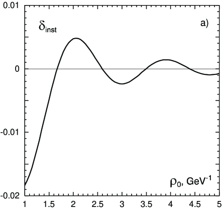
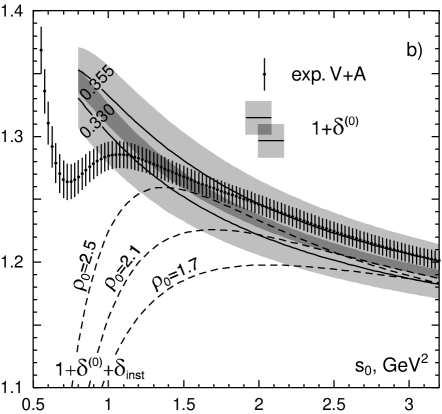
Figure 9: The instanton correction to the $\tau$ decay ratio versus $\rho_{0}$ (a) and ”versus $\tau$ mass” (b) for $n_{0}=1.5\times 10^{-3}\,{\rm GeV}^{4}$

As seen from Fig 9a the instanton correction to hadronic $\tau$-decay is extremely small except for unreliably low value of the instanton radius $\rho_{0}<1.5\,{\rm GeV}^{-1}$. At the favorable value [45] $\rho_{0}=1.7\,{\rm GeV}^{-1}$ the instanton correction to $R_{\tau}$ is almost exactly zero. (Of course, smaller values of $n_{0}$ than (45) are also allowed.) This fact confirms our calculations of $\alpha_{s}(m_{\tau}^{2})$ (Sec. 2), where the instanton corrections were not taken into account.

The result (47) can be used in another way. Namely, the $\tau$ mass can be considered as free parameter $s_{0}$. The dependence of the fractional corrections $\delta^{(0)}$ and $\delta^{(0)}_{0.330}+\delta_{\rm inst}$ on $s_{0}$ is shown in Fig 9b. The result strongly depends on the instanton radius and rather essentially on the density $n_{0}$. For $\rho_{0}=1.7\,{\rm GeV}^{-1}$ and $n_{0}=1\,{\rm fm}^{-4}$ (45) the instanton curve is outside the errors already at $s_{0}\sim 2\,{\rm GeV}^{2}$, where the perturbation theory is expected to work. Therefore Fig 9b shows, that in RILM model the instanton radius must be larger (say, $\rho_{0}=2.5\,{\rm GeV}^{-1}$) or the instanton density much ($2-3$ times) lower. The contribution of $D=6$ operator $\delta_{V+A}^{(6)}$ is not shown on Fig 9b. It is equal $\delta_{V+A}^{(6)}=-(5\pm 2)\times 10^{-3}(m_{\tau}^{6}/s_{0})^{3}$ and quite large at $s_{0}<1.5\,{\rm GeV}^{2}$.

Consequently in this approach the perturbation theory + OPE + RILM (at not very large $\rho_{0}$) cannot satisfactory describe the data at $s_{0}<1.5\,{\rm GeV}^{2}$. Since the instanton contribution is large here, we disbelieve all the results, obtained by the method of variable $\tau$-mass in this domain. (Perhaps, the shadowed region in Fig 3 is of importance in this method at low $s_{0}$.)

The $\tau$ decay ratio is not sensitive to the gluonic condensate. Let us consider now the sum rules which depend on it. The Borel transformation of the instanton part is:

$${\cal B}_{M^{2}}\Pi_{\rm inst} = 2\pi i\oint e^{-s/M^{2}}\,\Pi_{V,\,{\rm inst}}^{(1)}(s)\,{ds\over M^{2}}$$ (48)

$$= 4\pi^{2}\int_{0}^{\infty}\!d\rho\,n(\rho)\,\left[\,-\,{4\over 3M^{4}}\,+\,\sqrt{\pi}\rho^{4}G^{20}_{12}\left(\rho^{2}M^{2}\left|{1/2\atop 0,-2}\right.\right)\right]$$

The integration contour goes around the cut from $s=+\infty+i0$ to $s=+\infty-i0$. The term $\sim 1/M^{4}$ here comes from the term $\sim 1/q^{4}$ in (39); it must be included in the $\bigl{<}O_{4}\bigr{>}$ contribution in (26). The Meijer function in (48) has the asymptotics

$$G^{20}_{12}\left(z\left|{1/2\atop 0,-2}\right.\right)\,\approx\,z^{-5/2}e^{-z}\;,\qquad|z|\gg 1$$

and strongly suppressed at $M^{2}>0.8\,{\rm GeV}^{2}$. We calculated the instanton contribution to all Borel-like sum rules used here; it is indeed negligible compared to the errors. Consequently the results of previous sections remain unchanged.

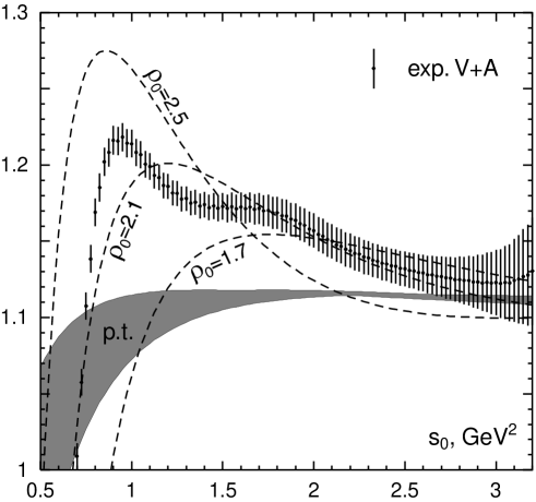
Figure 10: Sum rule (49). Experimental, pure perturbative and ”perturbative + instanton” parts are shown. The $O_{4}$ contribution is not taken into account.

However the spectral moments sum rules, often used in $\tau$-decay data analysis [1], can be quite sensitive to the instanton corrections. Let us consider the following sum rule, constructed in this way:

$$4\int_{0}^{s_{0}}{ds\over s_{0}}\,{s\over s_{0}}\left(1-{s^{2}\over s_{0}^{2}}\right)\omega_{\rm exp}(s)\,=\,{\rm p.t.}\,-\,8\pi^{2}{\bigl{<}O_{4}\bigr{>}\over s_{0}^{2}}\,+\,16\pi^{2}\int_{0}^{\infty}\!d\rho\,n(\rho)\,\rho^{4}\left[\,-{4\over 3\rho^{4}s_{0}^{2}}\right.\hskip 42.67912pt$$

$$\hskip 42.67912pt\left.+\sqrt{\pi}G^{21}_{24}\left(\rho^{2}s_{0}\left|{-1,1/2\atop 0,0,-2,-2}\right.\right)-\sqrt{\pi}G^{21}_{24}\left(\rho^{2}s_{0}\left|{-3,1/2\atop 0,0,-2,-4}\right.\right)\right]$$ (49)

The integral (49) is normalized to 1 in parton model. It does not depend on the $D=6$ operator, the factor $1-s^{2}/s_{0}^{2}$ is introduced to suppress large experimental errors for large $s_{0}$. Remind our convention: the contribution of the term $\sim 1/q^{4}$ in $\Pi_{\rm inst}$ (39) is included into the operator $\bigl{<}O_{4}\bigr{>}$ in (49). The contribution of different parts of eq. (49) are plotted versus $s_{0}$ in Fig 10. Since the weight function in the integral vanishes at $s=0$, the contribution of unphysical cut is suppressed. So the theoretical errors are diminished here as well as the sensitivity on various perturbative parameters. The theoretical curve is shown as single shaded area, which includes both the uncertainty of $\alpha_{s}(m_{\tau}^{2})$ and the error $\pm K_{3}a^{3}$ for each $\alpha_{s}(m_{\tau}^{2})$.

The operator $\bigl{<}O_{4}\bigr{>}$ enters with negative sign in (49), so the theoretical curve must go above experimental one. This is certainly not the case if the instanton corrections are not taken into account. For $\rho_{0}=2.1\,{\rm GeV}^{2}$ the theoretical and experimental results are in good agreement for $\bigl{<}O_{4}\bigr{>}=0$. By increasing the instanton density $n_{0}$, positive values of $\bigl{<}O_{4}\bigr{>}$ become possible. In this aspect sum rules (47) with varying $m_{\tau}$ and (49) are not in agreement: (47) favors small $n_{0}$ while (49) prefers large $n_{0}$.

These results are, however, not convincing. The main conclusion, coming from consideration of spectral moments sum rules, is that they are not suitable for QCD analysis untill we have a complete theory. (This statement surely refers also to the method, where $\tau$-mass is considered as free parameter.) The same situation took place for $V-A$ correlators: the spectral moments sum rules worked only at the circle radius $s_{0}>2\,{\rm GeV}^{2}$ [5].

8 Conclusion

The goal of this paper was to confront the recent precise experimental data on hadronic $\tau$-decay with QCD calculations at low $Q^{2}$ and to check the basic aspects of QCD: perturbative series, OPE as well as various nonperturbative QCD approaches. The data present the imaginary part of polarization operators ${\rm Im}\,\Pi_{V,A}(s)$, $s=q^{2}$ at $0<s<m_{\tau}^{2}$. If some procedure is applied to suppress or nullify the influence of high energy domain (Borel transformation, integration over closed circle in complex $s$-plane), then with help of dispersion relation the values of $\Pi_{V,A}(s)$ is the whole complex $s$-plane at low $|s|$ can be found from experiment. (By low $|s|$ we mean $|s|<2-3\,{\rm GeV}^{2}$.) These experimental values of $\Pi_{V,A}(s)$ can be compared with theoretical calculations in the domain of complex $s$-plane, where QCD describes the data well enough, in order to find the values of QCD parameters: $\alpha_{s}$ and condensates.

In [5] this program was realized for $\Pi_{V-A}$ polarization operator and the values of dimension 6 and 8 condensates were found. In this paper $\Pi_{V+A}$ and $\Pi_{V}$ polarization operators were studied, where perturbative contribution is dominant (unlike $\Pi_{V-A}$ which is given entirely by condensates). It must be stressed, that the present situation has changed drastically in comparison with earlier study of similar problem [4]. In [4] the perturbative contribution was much less essential and the authors could restrict theirselves to LO term only. In this paper the perturbative calculations were performed in 3 and 4 loop approximation. The unphysical cut in the complex $s$-plane in perturbative part of the polarization operator was taken into account and the calculations (at least partly) were performed in such a way, which allows one to minimize its influence (e.g. the Borel transformation along the rays, going from the origin at some angle). The terms of OPE were accounted up to dimension $D=8$. It was shown that $D=8$ contribution is very small in case of $V+A$ correlator. The coincidence of theoretical and experimental values with accuracy better than $2\%$ was required. Let us remind that usually the accuracy of standard QCD sum rule calculations is of order $10-15\%$.

The following results have been obtained:

1. The value of QCD coupling constant $\alpha_{s}(m_{\tau}^{2})=0.355\pm 0.025$ was found from hadronic branching ratio $R_{\tau}$. It was shown, the sum rules at low $|s|$ favor the value close to the lower error edge $\alpha_{s}(m_{\tau}^{2})=0.330$ corresponding to $\alpha_{s}(m_{Z}^{2})=0.118$.

2. It was demonstrated that QCD with inclusion of OPE terms is in agreement with the data at the values of complex Borel parameter $|M^{2}|>0.8-1.0\,{\rm GeV}^{2}$ in the left complex half-plane.

3. The restriction on the value of the gluonic condensate was found $\bigl{<}{\alpha_{s}\over\pi}G^{2}\bigr{>}=(0.006\pm 0.012)\,{\rm GeV}^{4}$ in comparison with standard SVZ value $0.012\,{\rm GeV}^{4}$.

4. The value of $D=6$ condensate found in [5] is in agreement with $V+A$ and $V$ sum rules, but cannot be specified.

5. The analytical perturbative QCD [32, 34, 36] was compared with the data and it was demonstrated that this approach is in strong contradiction with experimental value of $R_{\tau}$.

6. The restrictions on $1/Q^{2}$ term in polarization operator of renormalon origin were found, much stronger, than in the previous investigation [43].

7. The instanton contributions to polarization operator were analyzed and compared with the data in the framework of the random instanton liquid model (RILM) [45]. It was shown that the instanton contribution to $R_{\tau}$ is very small, the same is true for Borel sum rules. However their contributions can be significant to the spectral moments sum rules, often used in $\tau$-decay data analysis.

8. It was found that the method of spectral moments (integration over the circle with a polynomial) is less effective in the study of the polarization operators at low $Q^{2}$, than Borel sum rule because of larger contribution not given by OPE nonperturbative corrections (see Sec. 7 and [5]).

We believe, that the results of this paper will serve for improving the QCD sum rules method.

References

- [1] ALEPH collaboration: R. Barate et al, Eur.J.Phys. C4 (1998) 409. The data files are taken from http://alephwww.cern.ch/ALPUB/paper/paper.html
- [2] OPAL collaboration: K. Ackerstaff et al, Eur.J.Phys. C7 (1999) 571; G. Abbiendi et al, CERN EP/99-095, Eur.J.Phys.
- [3] CLEO collaboration: S.J. Richichi et al, Phys.Rev. D60 (1999) 112002
- [4] S.I. Eidelman, L.M. Kurdadze and A.I. Vainstein, Phys.Lett. B82 (1979) 278
- [5] B.L. Ioffe and K.N. Zyablyuk, Nucl.Phys. A (in press), hep-ph/0010089
- [6] J. Gasser and H. Leutwyler, Nucl.Phys. B250 (1985) 539
- [7] D.E. Groom et al, Eur.Phys.J. C15 (2000) 1
- [8] A. Pich, Proc. of QCD94 workshop, Monpellier, 1994, Nucl. Phys. Proc. Suppl. 39BC(1995) 326
- [9] W.J. Marciano, A. Sirlin, Phys.Rev.Lett. 61 (1998) 1815; 56 (1996) 22
- [10] E. Braaten, Phys.Rev.Lett. 60 (1988) 1606, Phys.Rev. D39 (1989) 1458
- [11] S.Narison and A. Pich, Phys.Lett. B211 (1988) 183
- [12] E.Braaten, S.Narison, A.Pich, Nucl.Phys. B373 (1992) 581
- [13] F.Le Diberder, A.Pich, Phys.Lett. B286 (1992) 147
- [14] K.G. Chetyrkin, A.L. Kataev and F.V. Tkachov, Phys. Lett. B85 (1979) 277; M. Dine and J. Sapirshtein, Phys. Rev. Lett. 43 (1979) 668; W. Celmaster and R. Gonsalves, ibid. 44 (1980) 560
- [15] L.R.Surgaladze, M.A.Samuel, Phys.Rev.Lett. 66 (1990) 560, e. ibid. 2416; S.G. Gorishny, A.L. Kataev and S.A. Larin, Phys.Lett. B259 (1991) 144
- [16] O.V. Tarasov, A.A. Vladimirov and A.Yu. Zharkov, Phys.Lett. B93 (1980) 429; S.A. Larin and J.A.M. Vermaseren, ibid. B303 (1993) 334
- [17] T. van Ritbergen, J.A.M. Vermaseren and S.A. Larin, Phys.Lett. B400 (1997) 379
- [18] B. Schrempp and F. Schrempp, Zs.Phys. C6 (1980) 7
- [19] A.V.Radyushkin, JINR E2-82-159, hep-ph/9907228
- [20] A. Pivovarov, Nuovo Cim. 105A (1992) 813
- [21] M.A. Shifman, A.I. Vainstein and V.I. Zakharov, Nucl.Phys. B147 (1979) 385
- [22] K.G. Chetyrkin, S.G. Gorishny and V.P. Spiridonov, Phys.Lett. B160 (1985) 149
- [23] L.-E. Adam and K.G. Chetyrkin, Phys.Lett. B329 (1994) 129
- [24] M.S. Dubovikov and A.V.Smilga, ITEP-82-42; Yad.Fiz. 37 (1983) 984
- [25] A. Grozin and Y. Pinelis, Phys.Lett. B166 (1986) 429
- [26] D.J. Broadhurst, S.C. Generalis, Phys.Lett. B165 (1985) 175
- [27] V.M. Belyaev and B.L. Ioffe, Sov.Phys. JETP 56 (1982) 493
- [28] ALEPH collaboration: R. Barate et al, Eur.Phys.J. C11 (1999) 599.
- [29] OPAL collaboration: G. Abbiendi et al, hep-ex/0009017
- [30] E. Braaten, C.S. Lee, Phys. Rev. D42 (1990) 3888
- [31] A.L. Kataev and V.V. Starchenko, Mod.Phys.Lett. A10 (1995) 235
- [32] D.V. Shirkov and I.L. Solovtsov, Phys.Rev.Lett. 79 (1997) 1204
- [33] I.L. Solovtsov and D.V. Shirkov, Phys.Lett. B442 (1998) 344; K.A. Milton and O.P. Solovtsova, Phys. Rev. D57 (1998) 5402; K.A. Milton, I.L. Solovtsov and O.P. Solovtsova, Phys. Rev. D60 (1999) 016001; A.V. Nesterenko, hep-ph/0102124, hep-ph/0102203
- [34] I.L. Solovtsov and D.V. Shirkov, Theor.Math.Phys. 120 (1999) 1210
- [35] K.A. Milton, I.L. Solovtsov and O.P. Solovtsova, Phys.Lett. B415 (1997) 104; K.A. Milton, I.L. Solovtsov and V.I. Yasnov, hep-ph/9802282
- [36] B.V. Geshkenbein and B.L. Ioffe, Pisma v ZhETF 70 (1999) 167
- [37] K.A. Milton, I.L. Solovtsov, O.P. Solovtsova, hep-ph/0102254
- [38] V.A. Novikov, M.A. Shifman, A. Vainshtein and V.I. Zakharov, Nucl.Phys. B249 (1985) 445
- [39] M.A. Shifman, Lecture at the 1997 Yukawa International Seminar: Non-Perturbative QCD-Structure of the QCD Vacuum, Kyoto, December 1997, Progr. Theor. Phys. Suppl. 131 (1998) 1, hep-ph/9802214
- [40] ALEPH collaboration: R. Barate et al, Z.Phys. C76 (1997) 15
- [41] M. Beneke, V. Braun, hep-ph/0010208
- [42] I. Suslov, ZhETF 116 (1999) 369
- [43] K.G. Chetyrkin, S. Narison, V.I. Zakharov, Nucl.Phys. B550 (1999) 353
- [44] C.A. Domingues, K. Schilcher, Phys.Rev. D61 (2000) 114020
- [45] T. Shafer, E.V. Shuryak, Rev.Mod.Phys. 70 (1998) 323
- [46] ”Instantons in Gauge Theories”, ed. by M. Shifman, World Scientific, 1994
- [47] N. Andrei, D.J. Gross, Phys. Rev. D18 (1978) 468
- [48] T. Shafer, E.V. Shuryak, hep-ph/0010116
- [49] Y.L. Luke, ”Mathematical functions and their approximations”, NY, Academic Press 1975; H. Bateman, A. Erdelyi, ”Higher transcendental functions”, Vol. I, NY, 1953