RADIATIVE CORRECTIONS
TO THE HIGGS BOSON MASS FOR A
HIERARCHICAL STOP SPECTRUM

An effective theory approach is used to compute analytically the radiative corrections to the mass of the light Higgs boson of the Minimal Supersymmetric Standard Model when there is a hierarchy in the masses of the stops ($M_{\tilde{t}_{1}}\gg M_{\tilde{t}_{2}}\gg M_{\mathrm{t}op}$, with moderate stop mixing). The calculation includes up to two-loop leading and next-to-leading logarithmic corrections dependent on the QCD and top-Yukawa couplings, and is further completed by two-loop non-logarithmic corrections extracted from the effective potential. The results presented disagree already at two-loop-leading-log level with widely used findings of previous literature. Our formulas can be used as the starting point for a full numerical resummation of logarithmic corrections to all loops, which would be mandatory if the hierarchy between the stop masses is large.

March 2001

IFT-UAM/CSIC-01-11

IEM-FT-214/01

hep-ph/0104047

1 Introduction

The Minimal Supersymmetric Standard Model (MSSM) predicts a light Higgs boson, with mass $M_{h^{0}}$ of the order of the scale of electroweak symmetry breaking ($G_{F}^{-1}\sim v=246$ GeV) times a small Higgs quartic-self-coupling. That Supersymmetry (SUSY) can naturally trigger this breaking, and stabilize the scale at which it takes place, is the most interesting part of the story (see [1] for reviews and references). Here we take that for granted and our focus is on the perturbatively small coupling. Its smallness comes about because of two reasons: first, Supersymmetry dictates that the Higgs quartic self-couplings are given by gauge couplings (from $D$-terms) and by superpotential Yukawa couplings (from $F$-terms); second, the latter $F$-term contributions are absent in the MSSM since, in this model, quantum numbers prevent superpotential terms cubic in the Higgs fields. It is generic [2] that quartic Higgs couplings are directly related to the Higgs mass after electroweak symmetry breaking (the Standard Model is the best known example). All this results in the well known tree-level upper bound $M_{h^{0}}^{2}\leq M_{Z}^{2}\cos^{2}2\beta$ [the SUSY parameter $\tan\beta$ is the ratio $v_{2}/v_{1}$ of the two Higgs vacuum expectation values (vevs). We follow the usual convention: $v_{2}$ generates the mass of the top quark and $v_{1}$ that of the bottom quark].

Radiative corrections to $M_{h^{0}}$ can be quite important because of top-stop loops that introduce a dependence on the top Yukawa coupling, $h_{t}$, which is sizeable, while this coupling does not enter in the tree-level Higgs mass. This can lead to cases in which one-loop radiative corrections to $M_{h^{0}}$ are comparable to, or even larger than the tree-level part of it (without this being an indication of the failure of the perturbative expansion).

In addition, the one-loop corrections to $M_{h^{0}}$ are logarithmically sensitive to the mass ratio, $m_{\tilde{t}}/m_{t}$, of the average stop mass over the top mass, which could be large if there is a hierarchy, $M_{SUSY}/M_{EW}\gg 1$, of the SUSY mass scale over the electroweak scale. As a consequence, radiative corrections to $M_{h^{0}}$ beyond one-loop can be important if $\ln(m_{\tilde{t}}/m_{t})$ is large. In that event, standard renormalization group (RG) techniques can be used with advantage to resum these logarithmic corrections to all loops.

During the last decade, the precise determination of $M_{h^{0}}$ as a function of the supersymmetric parameters has received continued attention [3]-[17]. The development of increasingly refined calculations of $M_{h^{0}}$ is the story of a stepwise climbing of this ladder of loop corrections and has been told elsewhere (see e.g. [15] for a brief account) so it will not be repeated here. The current status of what has been achieved, by the combined use of direct diagrammatic calculations, effective potential methods and RG techniques, could be summarized in this way: all one-loop corrections are known [5, 6] and the dominant two-loop corrections of order ${\cal O}(\alpha_{s}\alpha_{t}m_{t}^{2})$ and ${\cal O}(\alpha_{t}^{2}m_{t}^{2})$ are also known, including finite (non-logarithmic) contributions [here $\alpha_{s}\equiv g_{s}^{2}/(4\pi)$ and $\alpha_{t}\equiv h_{t}^{2}/(4\pi)$, with $g_{s}$ the QCD gauge coupling]. Higher order corrections at leading-log and next-to-leading-log order [${\cal O}(\alpha_{t}m_{t}^{2}\alpha_{t,s}^{n}[\ln(m_{\tilde{t}}/m_{t})]^{n})$ and ${\cal O}(\alpha_{t}m_{t}^{2}\alpha_{t,s}^{n+1}[\ln(m_{\tilde{t}}/m_{t})]^{n})$] can be resummed using one-loop and two-loop RG $\beta$-functions, respectively.

Beyond tree level, $M_{h^{0}}$ is sensitive to many SUSY parameters, but the most important are those of the stop sector (and of the sbottom sector also for large $\tan\beta$). They are given by the stop mass matrix:

$${\bf M}^{2}_{\tilde{t}}\ \simeq\ \left[\begin{array}[]{cc}M_{L}^{2}+m_{t}^{2}&m_{t}X_{t}\\[5.69054pt] m_{t}X_{t}^{*}&M_{R}^{2}+m_{t}^{2}\end{array}\right]\ ,$$ (1)

where we have neglected $D$-terms, $M_{L}^{2}$ ($M_{R}^{2}$) is the soft-mass for $\tilde{t}_{L}$ ($\tilde{t}_{R}$), and

$$X_{t}\equiv A_{t}+\mu^{*}/\tan\beta\ ,$$ (2)

with $A_{t}$ the soft trilinear coupling associated to the top Yukawa coupling and $\mu$ the supersymmetric Higgs mass in the superpotential.

The dependence of the radiative corrections to $M_{h^{0}}$ on these parameters has been studied before in different specific regimes. In this paper, we focus on the case in which there is a double hierarchy, $M_{L}\gg M_{R}\gg m_{t}$ (the case $M_{L}\gg M_{R}\simeq m_{t}$ can be worked out along similar lines). In this situation one should care, not only about potentially large logarithms like the usual $\ln(M_{L}/m_{t})$ and $\ln(M_{R}/m_{t})$, but also about $\ln(M_{L}/M_{R})$. Radiative corrections to $M_{h^{0}}$ for this type of stop spectrum have been considered in the past [11, 12] but there is room for improvement, as we will show. First, if the hierarchy between the stop masses is large, a numerical resummation of logarithmic corrections to all loops is necessary to get an accurate determination of the Higgs mass and, in order to do this, one has to identify first the relevant RG functions and threshold corrections. So far, this has not been done. Second, although previous analyses represent important steps ahead, they are not complete in one sense or another: either they do not include all potentially relevant corrections or, if they do, the corrections are not cast in a form suitable for RG resummation.

The plan of the paper is the following. In section 2 we present the main calculation. We use an effective theory method to extract and classify all two-loop dominant (i.e. $h_{t}$ and $g_{s}$-dependent) radiative corrections to $M_{h^{0}}$. The result of this calculation can be used as the starting point for a full numerical evaluation of the Higgs mass in the case of hierarchical stop spectra, although we do not undertake that task in this paper. In section 3, we discuss the possibility of finding a one-loop ‘improved’ approximation to $M_{h^{0}}$ that, playing with a judicious choice of the scales at which parameters are evaluated, tries to absorb higher order corrections. This exercise is a good point at which to compare our main result, presented in section 2, to previous analyses existing in the literature, with some of which we disagree already at the level of two-loop leading-log corrections. We dedicate section 4 to such comparisons. Section 5 presents our conclusions and outlook for future work. For reference, Appendix A presents an explicit formula for $M_{h^{0}}$ which includes up to two-loop-next-to-leading logarithmic corrections. Appendix B is devoted to the calculation of two-loop threshold corrections for the Higgs quartic self-coupling, of direct interest for the completeness of the two-loop calculation of $M_{h^{0}}$. Finally, Appendix C gives the relationships between $\overline{\rm MS}$  running parameters (in which our results are expressed) and on-shell (OS) quantities.

2 Effective theory calculation

We consider the MSSM with a particle spectrum in which all supersymmetric particles have a common mass, $M_{SUSY}$, much larger than the electroweak scale (say a few TeV) except for the lightest stop, which is much lighter although still heavier than the top quark. In particular, we remark that the mass of the pseudoscalar Higss, $M_{A^{0}}$, is also taken to be $M_{SUSY}$, and therefore, the model contains just one light Higgs doublet. To be precise, and referring to the stop mass matrix written in eq. (1), we consider

$$m_{t}\ll M_{R}\ll M_{L}=M_{SUSY}\ .$$ (3)

Concerning stop mixing, we also assume that it is not too large, so that it is a good approximation to say that the lightest stop is mostly $\tilde{t}_{R}$, while the heavier one is mainly $\tilde{t}_{L}$. In other words, we are in a situation in which the stop mixing angle is small. Nevertheless we do keep the dependence with the stop mixing parameter $X_{t}$ and we will derive our results as a series in powers of $m_{t}X_{t}/M_{L}^{2}$ (note that our approximation is $m_{t}X_{t}/M_{L}^{2}\ll 1$, not $X_{t}/M_{L}\ll 1$). The case of a hierarchy in stop masses due to very large $X_{t}$ (rather than to different diagonal soft masses) is worth separate study but it is more complicated and we do not consider it here.

To compute the radiatively corrected Higgs mass in the hierarchical case (3), we make use of an effective lagrangian approach, descending in energy from $M_{SUSY}$ down to the electroweak scale $m_{t}$. In doing so we encounter different effective theories at different energy scales. Above $M_{L}=M_{SUSY}$ the relevant theory is the full MSSM. Between $M_{L}=M_{SUSY}$ and $M_{R}$ the effective theory contains only the Standard Model particles with a single Higgs doublet (that particular rotation of the two Higgs doublets of the MSSM which is responsible for electroweak symmetry breaking and has SM properties) and, in addition, the light stop. Below the mass scale $M_{R}$ of that light stop the effective theory is simply the pure Standard Model (with calculable non-renormalizable operators, remnant of the decoupling of heavy SUSY particles).

To compute $M_{h^{0}}$ we start at $M_{SUSY}$ with the known value of the quartic Higgs coupling, $\lambda_{H}$, as a boundary condition fixed by Supersymmetry. We run this coupling down to $m_{t}$ in the different effective theories just mentioned, taking care of threshold corrections whenever some energy threshold is crossed. The procedure is standard and follows the general prescriptions for effective theory calculations. For general reviews of this subject we refer to [18] and references therein. We also found useful some general discussions in ref. [19], a more specialized paper which studies the effective theory of a linear $O(N)$ sigma model. Similar effective theory techniques have been applied to study the decoupling limit of the MSSM with heavy superpartners [20].

We work in an approximation that neglects in radiative corrections all couplings except $g_{s}$ and $h_{t}$ [our results could be extended easily to include also $h_{b}$ (bottom-Yukawa) corrections, which can be significant for large values of $\tan\beta$]. We keep electroweak gauge couplings only in the tree-level contribution to $M_{h^{0}}$. In this connection, the quartic Higgs coupling, $\lambda_{H}$, is considered to be itself of one-loop order [$\lambda_{H}\sim h_{t}^{4}/(16\pi^{2})$] when it appears in radiative corrections. Within this approximation, we plan to extract analytically the radiative corrections to $M_{h^{0}}$ up to two-loop order, that is, we compute one-loop leading-log and finite terms plus two-loop leading-log, next-to-leading-log and finite corrections to $M_{h^{0}}$. We also use, whenever necessary, expansions in powers of the mass ratios $m_{t}/M_{R}$, $m_{t}/M_{L}$ and $M_{R}/M_{L}$, as is common use in effective theory calculations. If these ratios are not small there is no necessity of using effective theory methods: the corresponding corrections to $M_{h^{0}}$ are not logarithmically enhanced and other existing calculations should be valid.

The analytical result for $M_{h^{0}}$ that we obtain in this way is interesting for two reasons: first, it identifies the ingredients (threshold corrections and renormalization group functions) necessary for a full numerical computation of the running of $\lambda_{H}$; second, it is interesting in order to develop simple and compact approximations to the full numerical results. Our goal is then to find a two-loop formula for the Higgs mass in which the corrections are classified in such a way as to permit a numerical resummation of leading and next-to-leading logarithmic corrections to all loops. As explained, this resummation is mandatory if the hierarchy (3) is sizeable, when simple analytical approximations start to fail. We defer that numerical evaluation of $M_{h^{0}}$ to a future publication and concentrate here upon the analytical study.

2.1 Plan

The method we follow is very similar to that used by Haber and Hempfling in ref. [9] to compute radiative corrections to $M_{h^{0}}$ for low values of the pseudoscalar mass, $M_{A^{0}}$, case in which the theory below $M_{SUSY}$ is a two-Higgs-doublet model. The plan of our calculation is to integrate the equation $d\lambda_{H}/d\ln Q^{2}=\beta_{\lambda_{H}}$ from $M_{SUSY}=M_{L}$, where $\lambda_{H}$ is related to SUSY parameters, to $M_{EW}=m_{t}$, where $\lambda_{H}$ determines the Higgs mass. Taking into account the different running in the two effective theories, above and below the intermediate threshold at $M_{R}$, and writing explicitly the threshold corrections to $\lambda_{H}$ [with a 0 superindex, as in $\lambda_{H}^{0}(M_{L})$, we always indicate a tree-level value], we find

$$\lambda(m_{t}) = \lambda_{H}^{0}(M_{L})+\delta\lambda_{H}(M_{L})-\int_{Q=m_{t}}^{M_{R}^{-}}\beta_{\lambda}(Q)d\ln Q^{2}$$ (4)

$$+\delta\lambda_{H}(M_{R})-\int_{Q=M_{R}^{+}}^{M_{L}}\beta_{\lambda_{H}}(Q)d\ln Q^{2}\ .$$

The quantities $\delta\lambda_{H}$ are the threshold corrections for $\lambda_{H}$ at the indicated scales. We call $\lambda$ the Higgs quartic coupling below $M_{R}$ to distinguish it from $\lambda_{H}$ above $M_{R}$.

If we next expand the $\beta$-functions around a particular value of the scale, and make a loop expansion up to two-loops [$\beta=\beta^{(1)}+\beta^{(2)}+...$] we get

$$\lambda(m_{t}) = \lambda_{H}(M_{L})+\delta\lambda_{H}(M_{L})+\delta\lambda_{H}(M_{R})$$ (5)

$$-\left[\beta_{\lambda}^{(1)}(m_{t})+\beta_{\lambda}^{(2)}\right]\ln{M_{R}^{2}\over m_{t}^{2}}-\left[\beta_{\lambda_{H}}^{(1)}(M_{R})+\beta_{\lambda_{H}}^{(2)}\right]\ln{M_{L}^{2}\over M_{R}^{2}}$$

$$-{1\over 2}{d\beta_{\lambda}^{(1)}\over d\ln Q^{2}}\ln^{2}{M_{R}^{2}\over m_{t}^{2}}-{1\over 2}{d\beta_{\lambda_{H}}^{(1)}\over d\ln Q^{2}}\ln^{2}{M_{L}^{2}\over M_{R}^{2}}+...$$

It is important to make explicit the scale at which one-loop $\beta$-functions are evaluated, because different scale choices amount to a two-loop difference [the scale choice in two-loop terms like $\beta^{(2)}$ or $d\beta^{(1)}/d\ln Q^{2}$ has only effects starting at three loops]. The same comments apply to the choice of the scale at which to evaluate the masses inside one-loop logarithms. In (5), the RG procedure dictates that they are evaluated at a scale equal to the mass itself, that is, $M_{R}\equiv M_{R}(M_{R})$, $M_{L}\equiv M_{L}(M_{L})$ and $m_{t}\equiv\overline{m}_{t}(m_{t})$. In a similar way, it is important that the couplings which appear in $\beta^{(1)}$’s are evaluated taking into account the corresponding one-loop threshold corrections. All this will be shown more explicitly in the following subsections.

Eq. (5) already illustrates some properties of radiative corrections which are generic: i) Leading-log contributions at any order depend only on one-loop RG-functions and are, therefore, insensitive to threshold corrections and two-loop or higher RG-functions. The reason is simple: by definition, in leading-log corrections each power of the loop expansion parameter $\alpha$ ($\alpha_{t}$ or $\alpha_{s}$ in our case) is accompanied by a logarithm (that arises from RG running between two mass scales). However, threshold corrections introduce powers of $\alpha$’s without such logarithms, while $n^{th}$-order RG-functions introduce a factor $\alpha^{n-1}$ for each $\alpha\log$. ii) Next-to-leading-log terms are instead sensitive first to two-loop RG-functions and second, to one-loop RG-functions times one-loop threshold corrections. In turn, they are not sensitive to three-loop (or higher) RG-functions or two-loop (or higher) threshold corrections.

With this hierarchical classification of radiative corrections in mind, our calculation aims at finding the relevant one and two-loop RG-functions plus one-loop threshold corrections. This would allow the resummation of leading and next-to leading logarithmic contributions to $M_{h^{0}}$ to all loops. Nevertheless, in our analytical formulas we stop at two-loops, including also two-loop non-logarithmic terms.

2.2 SUSY threshold: matching MSSM with SM $+$ $\tilde{t}_{R}$

The effective theory below the supersymmetric threshold at $M_{SUSY}$ is described by the most general Lagrangian built with SM particles plus $\tilde{t}_{R}$, non-renormalizable in general but invariant under the $SU(3)_{C}\times SU(2)_{L}\times U(1)_{Y}$ gauge symmetry:

$${\cal L}_{SM+\tilde{t}_{R}} = ({\cal D}_{\mu}\tilde{t}_{R})^{\alpha\dagger}({\cal D}^{\mu}\tilde{t}_{R})^{\alpha}+({\cal D}_{\mu}\lower 5.16663pt\hbox{$\stackrel{{\scriptstyle\textstyle h}}{{\footnotesize\sim}}$})^{\dagger}({\cal D}^{\mu}\lower 5.16663pt\hbox{$\stackrel{{\scriptstyle\textstyle h}}{{\footnotesize\sim}}$})-\overline{M}_{R}^{2}|\tilde{t}_{R}|^{2}-\overline{m}^{2}|\lower 5.16663pt\hbox{$\stackrel{{\scriptstyle\textstyle h}}{{\footnotesize\sim}}$}|^{2}$$ (6)

$$+[g_{t}Q_{L}^{\alpha}c\,t_{R}^{c\alpha}\cdot\lower 5.16663pt\hbox{$\stackrel{{\scriptstyle\textstyle h}}{{\footnotesize\sim}}$}+{\mathrm{h}.c.}]-{1\over 2}\lambda_{U}|\tilde{t}_{R}|^{4}-{1\over 2}\lambda_{H}|\lower 5.16663pt\hbox{$\stackrel{{\scriptstyle\textstyle h}}{{\footnotesize\sim}}$}|^{4}-\lambda_{HU}|\tilde{t}_{R}|^{2}|\lower 5.16663pt\hbox{$\stackrel{{\scriptstyle\textstyle h}}{{\footnotesize\sim}}$}|^{2}$$

$$-\lambda_{HU}^{\prime}(\tilde{t}_{R}^{\alpha*}\lower 5.16663pt\hbox{$\stackrel{{\scriptstyle\textstyle h}}{{\footnotesize\sim}}$})\cdot\partial^{2}(\overline{\lower 5.16663pt\hbox{$\stackrel{{\scriptstyle\textstyle h}}{{\footnotesize\sim}}$}}\tilde{t}_{R}^{\alpha})-\kappa^{2}|\tilde{t}_{R}|^{2}|\lower 5.16663pt\hbox{$\stackrel{{\scriptstyle\textstyle h}}{{\footnotesize\sim}}$}|^{4}-\chi|\lower 5.16663pt\hbox{$\stackrel{{\scriptstyle\textstyle h}}{{\footnotesize\sim}}$}|^{2}|\tilde{t}_{R}|^{4}+...\ ,$$

where the ellipsis stands for terms of higher order both in fields (bosonic or fermionic) and derivatives. The Higgs doublet field is represented by $\stackrel{{\scriptstyle\textstyle h}}{{\footnotesize\sim}}$, $Q_{L}^{\alpha}$ is the top-bottom quark doublet and $t_{R}^{\alpha}$ the right-handed top quark field ($\alpha$ is a colour index). The dot ($\cdot$) stands for the $SU(2)$ invariant product and $c=-i\sigma^{2}$. We have written explictly only the third generation Yukawa coupling, which in this intermediate-energy theory we call $g_{t}$. We keep only terms directly related to our calculation and do not write, for example, fermion kinetic terms.

The parameters in the Lagrangian (6) are determined by matching at the scale $Q=M_{SUSY}$ with the full MSSM theory, i.e. by requiring that the effective theory and the full MSSM give the same physics at low momentum [18]. To do this matching at tree level, we first obtain the equations of motion of the heavy MSSM fields and substitute them (making a low momentum expansion) in the MSSM Lagrangian. What one obtains is (we use a prime to distinguish this Lagrangian from that of the MSSM with heavy fields not replaced by their equations of motion)

$${\cal L}^{\prime}_{MSSM} = ({\cal D}_{\mu}\tilde{t}_{R})^{\alpha\dagger}({\cal D}^{\mu}\tilde{t}_{R})^{\alpha}+({\cal D}_{\mu}\lower 5.16663pt\hbox{$\stackrel{{\scriptstyle\textstyle h}}{{\footnotesize\sim}}$})^{\dagger}({\cal D}^{\mu}\lower 5.16663pt\hbox{$\stackrel{{\scriptstyle\textstyle h}}{{\footnotesize\sim}}$})-M_{R}^{2}|\tilde{t}_{R}|^{2}-m^{2}|\lower 5.16663pt\hbox{$\stackrel{{\scriptstyle\textstyle h}}{{\footnotesize\sim}}$}|^{2}$$ (7)

$$-h_{t}^{2}s_{\beta}^{2}|\tilde{t}_{R}|^{2}|\lower 5.16663pt\hbox{$\stackrel{{\scriptstyle\textstyle h}}{{\footnotesize\sim}}$}|^{2}-{1\over 2}g_{s}^{2}\sum_{a}(\tilde{t}_{R}^{\alpha*}T^{a}_{\alpha\beta}\tilde{t}_{R}^{\beta})^{2}-{1\over 8}g^{2}\sum_{a}(\lower 5.16663pt\hbox{$\stackrel{{\scriptstyle\textstyle h}}{{\footnotesize\sim}}$}^{\dagger}\sigma^{a}\lower 5.16663pt\hbox{$\stackrel{{\scriptstyle\textstyle h}}{{\footnotesize\sim}}$})^{2}$$

$$-{1\over 72}{g^{\prime}}^{2}\left[4|\tilde{t}_{R}|^{2}+3c_{2\beta}|\lower 5.16663pt\hbox{$\stackrel{{\scriptstyle\textstyle h}}{{\footnotesize\sim}}$}|^{2}\right]^{2}+[h_{t}s_{\beta}Q_{L}^{\alpha}c\,t_{R}^{c\alpha}\cdot\lower 5.16663pt\hbox{$\stackrel{{\scriptstyle\textstyle h}}{{\footnotesize\sim}}$}+{\mathrm{h}.c.}]$$

$$+h_{t}^{2}s_{\beta}^{2}|X_{t}|^{2}(\tilde{t}_{R}^{\alpha*}\lower 5.16663pt\hbox{$\stackrel{{\scriptstyle\textstyle h}}{{\footnotesize\sim}}$})\cdot P_{L}(\partial^{2})(\overline{\lower 5.16663pt\hbox{$\stackrel{{\scriptstyle\textstyle h}}{{\footnotesize\sim}}$}}\tilde{t}_{R}^{\alpha})+h_{t}^{4}s_{\beta}^{2}c_{\beta}^{2}|\tilde{t}_{R}|^{2}\lower 5.16663pt\hbox{$\stackrel{{\scriptstyle\textstyle h}}{{\footnotesize\sim}}$}\cdot P_{A}(\partial^{2})\overline{\lower 5.16663pt\hbox{$\stackrel{{\scriptstyle\textstyle h}}{{\footnotesize\sim}}$}}|\tilde{t}_{R}|^{2}$$

$$+h_{t}^{2}s_{\beta}^{2}g_{s}^{2}(T^{a}_{\alpha\beta}T^{a}_{\rho\eta}-h_{t}^{2}\delta_{\rho\alpha}\delta_{\eta\beta})|X_{t}|^{2}(\tilde{t}_{R}^{\alpha*}\lower 5.16663pt\hbox{$\stackrel{{\scriptstyle\textstyle h}}{{\footnotesize\sim}}$})\cdot P_{L}(\partial^{2})\tilde{t}_{R}^{\rho*}\tilde{t}_{R}^{\eta}P_{L}(\partial^{2})(\overline{\lower 5.16663pt\hbox{$\stackrel{{\scriptstyle\textstyle h}}{{\footnotesize\sim}}$}}\tilde{t}_{R}^{\beta})$$

$$-h_{t}^{4}s_{\beta}^{4}|X_{t}|^{2}\left[\tilde{t}_{R}^{\alpha*}\lower 5.16663pt\hbox{$\stackrel{{\scriptstyle\textstyle h}}{{\footnotesize\sim}}$}\cdot P_{L}(\partial^{2})\overline{\lower 5.16663pt\hbox{$\stackrel{{\scriptstyle\textstyle h}}{{\footnotesize\sim}}$}}\right]\left[\lower 5.16663pt\hbox{$\stackrel{{\scriptstyle\textstyle h}}{{\footnotesize\sim}}$}\cdot P_{L}(\partial^{2})\overline{\lower 5.16663pt\hbox{$\stackrel{{\scriptstyle\textstyle h}}{{\footnotesize\sim}}$}}\tilde{t}_{R}^{\alpha}\right]$$

$$-\left[h_{t}^{4}c_{\beta}^{2}s_{\beta}^{2}X_{t}Y_{t}^{*}(\tilde{t}_{R}^{\alpha*}\lower 5.16663pt\hbox{$\stackrel{{\scriptstyle\textstyle h}}{{\footnotesize\sim}}$})\cdot P_{L}(\partial^{2})\tilde{t}_{R}^{\alpha}P_{A}(\partial^{2})\overline{\lower 5.16663pt\hbox{$\stackrel{{\scriptstyle\textstyle h}}{{\footnotesize\sim}}$}}|\tilde{t}_{R}|^{2}+{\mathrm{h}.c.}\right]$$

$$+h_{t}^{4}c_{\beta}^{2}s_{\beta}^{2}|X_{t}Y_{t}|^{2}(\tilde{t}_{R}^{\alpha*}\lower 5.16663pt\hbox{$\stackrel{{\scriptstyle\textstyle h}}{{\footnotesize\sim}}$})\cdot P_{L}(\partial^{2})\tilde{t}_{R}^{\alpha}P_{A}(\partial^{2})\tilde{t}_{R}^{\beta*}P_{L}(\partial^{2})\overline{\lower 5.16663pt\hbox{$\stackrel{{\scriptstyle\textstyle h}}{{\footnotesize\sim}}$}}\tilde{t}_{R}^{\beta}$$

$$+{1\over 2}\left[h_{t}^{2}\tilde{t}_{R}^{\alpha*}Q_{Li}^{\alpha T}i{\overline{\sigma}^{\mu}}^{T}\partial_{\mu}P_{\tilde{H}}(\partial^{2})(\tilde{t}_{R}^{\beta}Q_{Li}^{\beta*})+{\mathrm{h}.c.}\right]$$

$$-\left\{g_{s}^{2}T^{a}_{\alpha\beta}T^{a}_{\rho\eta}\tilde{t}_{R}^{\alpha*}t_{R}^{c\beta T}\left[M_{G}P_{G}(\partial^{2})c\ t_{R}^{c\rho}\tilde{t}_{R}^{\eta*}+i\sigma_{\mu}\partial^{\mu}P_{G}(\partial^{2})t_{R}^{c\eta*}\tilde{t}_{R}^{\rho}\right]+{\mathrm{h}.c.}\right\}$$

$$-h_{t}^{2}c_{\beta}^{2}P_{A}(\partial^{2})(Q_{Li}^{\alpha\dagger}ct_{R}^{c\alpha*})(Q_{Li}^{\beta T}c\ t_{R}^{c\beta})+...$$

where $g$ and $g^{\prime}$ are the $SU(2)_{L}$ and $U(1)_{Y}$ coupling constants respectively; $\overline{\lower 5.16663pt\hbox{$\stackrel{{\scriptstyle\textstyle h}}{{\footnotesize\sim}}$}}$ is the $SU(2)$ conjugate of the light Higgs field $\stackrel{{\scriptstyle\textstyle h}}{{\footnotesize\sim}}$; $c_{\beta}=\cos\beta$, $s_{\beta}=\sin\beta$; $\overline{\sigma}^{\mu}=(1,-\vec{\sigma})$; $T^{a}_{\alpha\beta}$ are the $SU(3)_{C}$ generators in the fundamental representation; and

$$Y_{t}\equiv A_{t}-\mu^{*}\tan\beta\ .$$ (8)

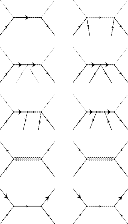
Figure 1: Tree-level diagrams, with heavy supersymmetric particles interchanged, that give rise to different terms of the Lagrangian (7).

Figure 2: One-loop diagram that cancels when all the components of $SU(2)$ doublets run in the loop.

We have written $\overline{M}_{R}^{2}$ and $\overline{m}^{2}$ in ${\cal L}_{SM+\tilde{t}_{R}}$ to distinguish them from ${M}_{R}^{2}$ and ${m}^{2}$ in ${\cal L}^{\prime}_{MSSM}$. We have also introduced the operators

$$P_{x}(\partial^{2})\equiv\left[{1\over M_{x}^{2}+\partial^{2}}\right]_{E}\ ,$$ (9)

for $x={L,A,\tilde{H},G}$ (corresponding to the soft mass $M_{L}$ of $\tilde{t}_{L}$, the pseudoscalar mass $M_{A}$, the higgsino mass $M_{\tilde{H}}^{2}=|\mu|^{2}$ and the gluino mass $M_{G}^{2}$, respectively). In eq. (9) the subindex $E$ indicates a low-momentum expansion in powers of $\partial^{2}/M_{x}^{2}$. In (7), these operators act only inside the square brackets they are in.

Figure 3: One-loop diagrams for the threshold correction to $\lambda_{H}$ in the full MSSM.

Figure 4: One-loop diagrams for the threshold correction to the quartic Higgs coupling $\lambda_{H}$ in the effective theory SM $+$ $\tilde{t}_{R}$.

The origin of each non-renormalizable term in ${\cal L}^{\prime}_{MSSM}$ [eq. (7)] is easy to interpret as coming from the tree-level exchange of one or more heavy particles [identified by the propagator operators $P_{x}(\partial^{2})$]. This is shown diagrammatically in figure 1, which shows the tree-level diagrams that give rise to the different terms of (7), upon collapsing heavy particle lines to a point. The line code we use is the following: a thin dashed line with a small arrow [which indicates the flow of SU(2) quantum numbers] represents the light Higgs doublet; the same type of line but with double dash corresponds to the heavy Higgs doublet; a double continuous line with an $SU(2)$ arrow represents a Higgsino; a dashed bold line with a large arrow [indicating $SU(3)$ colour flow] represents a light stop; the same type of line but thicker and with a larger arrow [which indicates the flow of $SU(2)$ and $SU(3)$ quantum numbers] is used for the heavy stop; gluinos are represented by a continuous line with a wiggle; a top-bottom quark doublet is represented by a solid line with a large arrow, while the same type of line with a smaller arrow corresponds to a right-handed top quark. For our calculations and diagrams we work in the unbroken-symmetry phase, with the full $SU(2)$ doublet structure unresolved. This simplifies our task: when dealing with separate diagrams for the different components of a doublet there are cancellations, due to $SU(2)$ symmetry, which are immediately obvious in our approach. One such example is the diagram of figure 2. There is a cancellation between the contributions of different $SU(2)$ doublet components running in the loop. If one works with complete $SU(2)$ multiplets, this cancellation is reflected in the impossibility of drawing such a diagram properly: there is no choice for the arrow of the heavy Higgs field in the loop that is consistent with the flow of $SU(2)$ quantum numbers through other lines of the diagram.

Comparing ${\cal L}^{\prime}_{MSSM}$ [eq. (7)] to ${\cal L}_{SM+\tilde{t}_{R}}$ [eq. (6)], we get the tree-level matching conditions:

$$\lambda_{H}(M_{L}) = {1\over 4}(g^{2}+{g^{\prime}}^{2})\cos^{2}2\beta+\delta\lambda_{H}(M_{L})\ ,$$

$$\lambda_{HU}(M_{L}) = g_{t}^{2}-g_{t}^{2}{|X_{t}|^{2}\over M_{L}^{2}}+{1\over 3}{g^{\prime}}^{2}\cos 2\beta+\delta\lambda_{HU}(M_{L})\ ,$$

$$\lambda_{U}(M_{L}) = {1\over 3}g_{s}^{2}+{4\over 9}{g^{\prime}}^{2}+\delta\lambda_{U}(M_{L})\ ,$$

$$g_{t}(M_{L}) = h_{t}\sin\beta+\delta g_{t}(M_{L})\ ,$$

$$\overline{M}_{R}^{2}(M_{L}) = M_{R}^{2}+\delta\overline{M}_{R}^{2}(M_{L})\ ,$$ (10)

where we have just indicated the presence of loop corrections and, with an abuse of notation, used $g_{t}=h_{t}\sin\beta$ everywhere. In addition, we list the following tree-level threshold values for some non-renormalizable couplings in ${\cal L}_{SM+\tilde{t}_{R}}$ which will play a role in higher loop calculations:

$$\lambda^{\prime}_{HU}(M_{L}) = g_{t}^{2}{|X_{t}|^{2}\over M_{L}^{4}}+\delta\lambda^{\prime}_{HU}(M_{L})\ ,$$

$$\kappa^{2}(M_{L}) = g_{t}^{4}{|X_{t}|^{2}\over M_{L}^{4}}+\delta\kappa^{2}(M_{L})\ ,$$

$$\chi(M_{L}) = \left({1\over 3}g_{s}^{2}-h_{t}^{2}\right){|X_{t}|^{2}\over M_{L}^{4}}+{h_{t}^{2}c_{\beta}^{2}\over M_{A}^{2}}\left|1-{X_{t}Y_{t}^{*}\over M_{L}^{2}}\right|^{2}+\delta\chi(M_{L})\ .$$ (11)

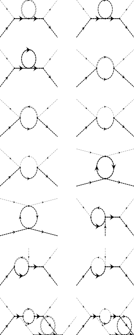
Figure 5: One-loop diagrams for the threshold correction to the Higgs-stop coupling $\lambda_{HU}$ in the full MSSM.

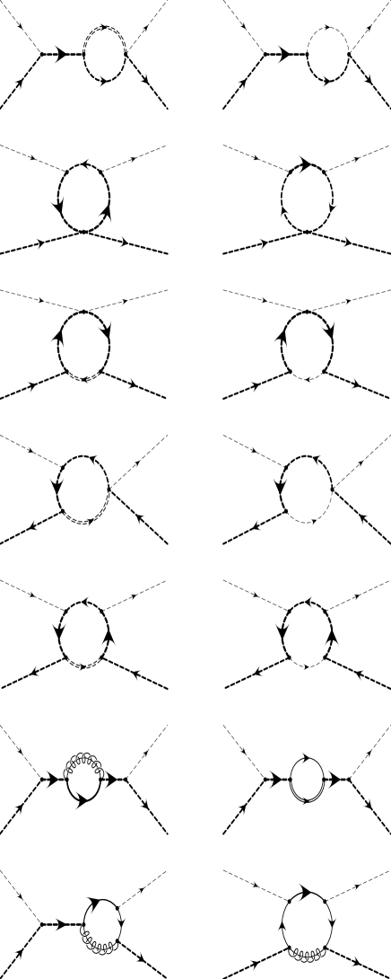
Figure 6: One-loop diagrams for the threshold correction to the Higgs-stop coupling $\lambda_{HU}$ in the full MSSM (continued).

Figure 7: One-loop diagrams for the threshold correction to the Higgs-stop coupling $\lambda_{HU}$ in the effective theory SM $+$ $\tilde{t}_{R}$.

Figure 8: One-loop diagram for the threshold correction to the top Yukawa coupling in the full MSSM.

This tree-level matching would be enough if we were only after leading-log corrections to $M_{h^{0}}$ (which are not sensitive to threshold corrections). As we have discussed already, if we want to correctly obtain next-to-leading log contributions, this matching must be done at one-loop level. That is, we need the one-loop threshold corrections in the matching conditions (10). To compute them we match the one-loop effective actions in both theories, MSSM and SM $+$ $\tilde{t}_{R}$. Again, to do this, we first substitute in the MSSM effective action the equations of motion of heavy fields in a local momentum expansion. In other words, we match 1LPI (one-light-particle-irreducible) graphs with light-particle external legs in both theories. This procedure leads to the one loop threshold corrections:

$$\delta_{0}\lambda_{H}(M_{L}) = {N_{c}\over 8\pi^{2}}g_{t}^{4}{|X_{t}|^{4}\over M_{L}^{4}}\left[1+3{M_{R}^{2}\over M_{L}^{2}}+{\cal O}\left({M_{R}^{4}\over M_{L}^{4}}\right)\right]\ ,$$ (12)

$$\delta_{0}\lambda_{HU}(M_{L}) = {g_{t}^{2}\over 8\pi^{2}}\left\{2g_{s}^{2}C_{2}(N_{c})\left[1+2M_{G}{X_{t}+h.c.\over M_{L}^{2}}\right]\right.$$

$$+h_{t}^{2}\left[s_{\beta}^{2}+(1+2s_{\beta}^{2}+N_{c}){|X_{t}|^{2}\over M_{L}^{2}}+s_{\beta}^{2}{|X_{t}|^{4}\over M_{L}^{4}}\right.$$

$$\left.\left.+c_{\beta}^{2}{Y_{t}X_{t}^{*}+h.c.\over M_{L}^{2}}+c_{\beta}^{2}{|Y_{t}|^{2}\over 4M_{L}^{2}}-3c_{\beta}^{2}{|X_{t}Y_{t}|^{2}\over 4M_{L}^{4}}\right]\right\}+{\cal O}\left({M_{R}^{2}\over M_{L}^{2}}\right)\ ,$$

$$\delta_{0}g_{t}(M_{L}) = -{g_{t}g_{s}^{2}\over 8\pi^{2}}C_{2}(N_{c}){M_{G}\over M_{L}^{2}}X_{t}+{\cal O}\left({M_{R}^{2}\over M_{L}^{2}}\right)\ ,$$ (14)

$$\delta_{0}M_{R}^{2}(M_{L}) = {g_{s}^{2}\over 4\pi^{2}}C_{2}(N_{c})M_{S}^{2}+{g_{t}^{2}\over 8\pi^{2}}(M_{S}^{2}-|X_{t}|^{2})\ ,$$ (15)

Here, $N_{c}=3$ is the number of colours and $C_{2}(N_{c})=(N_{c}^{2}-1)/(2N_{c})$ is the quadratic Casimir of the fundamental representation of $SU(N_{c})$. For simplicity in our notation, we remove the bar from $\overline{M}_{R}$ in these equations and from now on, in the understanding that $M_{R}$ is, in what follows, the parameter of the intermediate-energy theory.

These results are approximations in which we have neglected all couplings other than the top Yukawa coupling and the strong gauge coupling. They are expansions in powers of $M_{R}/M_{L}$ to the indicated order of approximation. We have truncated the expansions in such a way as to reproduce the correct one-loop corrections to $M_{h^{0}}$ up to and including ${\cal O}(M_{R}^{2}/M_{L}^{2})$ terms while we neglect this type of corrections in the two-loop contributions [for that reason we need to keep ${\cal O}(M_{R}^{2}/M_{L}^{2})$ corrections only to $\lambda_{H}$, which enters $M_{h^{0}}$ already at tree level]. In addition, we have used the assumed identity of different heavy masses ($M_{A}=M_{\tilde{H}}=M_{G}=M_{L}$) to simplify the expressions (although we leave explicit linear terms in $M_{G}$ to allow for possible sign effects related to that mass).

In figure 3 we give the 1LPI diagrams that contribute to $\lambda_{H}$ at one loop in the full MSSM, while figure 4 shows the corresponding diagrams in the SM $+$ $\tilde{t}_{R}$ theory. Couplings in this last figure are distinguished from those in figure 3 by a black square to represent that they already include tree-level matching corrections. The one-loop threshold correcction $\delta\lambda_{H}$ is given by the contribution of the diagrams of figure 3 minus the contribution of the diagrams of figure 4. We therefore omit from these figures those diagrams that would be exactly equal in both theories (such diagrams do not contribute to the threshold correcction $\delta\lambda_{H}$) or diagrams that are simply zero.

In a similar way, figures 5 and 6 give the 1LPI diagrams that contribute to $\lambda_{HU}$ at one loop in the full MSSM, while figure 7 shows the corresponding 1LPI diagrams in the SM $+$ $\tilde{t}_{R}$ theory. At the order we work, the only diagrams that contribute to the threshold corrections of the top Yukawa coupling, $g_{t}$, and of the mass $M_{R}$ of the light stop $\tilde{t}_{R}$, are diagrams in the full MSSM. They are shown in figure 8 for $g_{t}$, and in figure 9 for $M_{R}$.

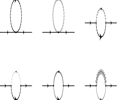
Figure 9: One-loop diagrams for the threshold correction to the mass and wave-function of $\tilde{t}_{R}$ in the full MSSM.

Figure 10: One-loop diagrams for the threshold correction to the wave-function of the light Higgs $\stackrel{{\scriptstyle\textstyle h}}{{\footnotesize\sim}}$ in the full MSSM and the effective theory SM $+$ $\tilde{t}_{R}$.

Figure 11: One-loop diagrams for the threshold correction to the wave-function of the left-handed top quark in the full MSSM and the effective theory SM $+$ $\tilde{t}_{R}$.

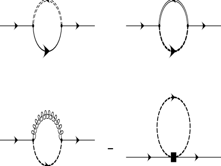
Figure 12: One-loop diagrams for the threshold correction to the wave-function of the right-handed top quark in the full MSSM and the effective theory SM $+$ $\tilde{t}_{R}$.

The subindex $0$ in eq. (15) is meant to indicate that these are not the final one-loop threshold corrections: there are also threshold corrections to kinetic terms and, after redefining the fields to get canonical kinetic terms, the results in eq. (15) are also affected and one finally gets

$$\delta_{1}\lambda_{H}(M_{L}) = \delta_{0}\lambda_{H}(M_{L})-2\lambda_{H}\delta Z_{H}\ ,$$

$$\delta_{1}\lambda_{HU}(M_{L}) = \delta_{0}\lambda_{HU}(M_{L})-\lambda_{HU}(\delta Z_{U}+\delta Z_{H})\ ,$$

$$\delta_{1}g_{t}(M_{L}) = \delta_{0}g_{t}(M_{L})-{1\over 2}g_{t}\left(\delta Z_{t_{L}}+\delta Z_{t_{R}}+\delta Z_{H}\right)+\Delta_{\mbox{\footnotesize$\overline{\rm DR}$~{}}\rightarrow\mbox{\footnotesize$\overline{\rm MS}$~{}}}\ ,$$

$$\delta_{1}M_{R}^{2}(M_{L}) = \delta_{0}M_{R}^{2}(M_{L}^{2})-M_{R}^{2}\delta Z_{U}\ ,$$ (16)

with wave-function threshold corrections encoded in

$$\delta Z_{t_{L}} = {h_{t}^{2}\over 64\pi^{2}}(3+c_{\beta}^{2})\ ,$$

$$\delta Z_{t_{R}} = {3g_{s}^{2}\over 32\pi^{2}}C_{2}(N_{c})+{h_{t}^{2}\over 32\pi^{2}}c_{\beta}^{2}\ ,$$

$$\delta Z_{H} = {3g_{t}^{2}\over 32\pi^{2}}|X_{t}|^{2}\ ,$$

$$\delta Z_{U} = {g_{s}^{2}\over 16\pi^{2}}C_{2}(N_{c})+{h_{t}^{2}\over 16\pi^{2}}\left(1+{|X_{t}|^{2}\over M_{L}^{2}}s_{\beta}^{2}+{1\over 3}{|Y_{t}|^{2}\over M_{L}^{2}}c_{\beta}^{2}\right)\ ,$$ (17)

for $Q_{L}^{\alpha}$, $t_{R}^{\alpha}$, $\stackrel{{\scriptstyle\textstyle h}}{{\footnotesize\sim}}$ and $\tilde{t}_{R}$ fields, respectively. We have also added a term (see [21])

$$\Delta_{\mbox{\footnotesize$\overline{\rm DR}$~{}}\rightarrow\mbox{\footnotesize$\overline{\rm MS}$~{}}}={g_{t}g_{s}^{2}\over 16\pi^{2}}C_{2}(N_{c})\ ,\\$$ (18)

to correct from the change of scheme, from $\mbox{\footnotesize$\overline{\rm DR}$~{}}^{\prime}$ (the modified $\overline{\rm DR}$  scheme of [22]) in the MSSM to $\overline{\rm MS}$ , which is the scheme we use below the supersymmetric threshold.

The diagrams that contribute to the threshold corrections to kinetic terms, given in (17), are shown in figure 9, for $\tilde{t}_{R}$; in figure 10 for $\stackrel{{\scriptstyle\textstyle h}}{{\footnotesize\sim}}$; in figure 11 for $t_{L}$ and in figure 12 for $t_{R}$. In the last three figures we give together the diagrams in the full theory and (with a minus sign in front) those in the effective theory (SM $+$ $\tilde{t}_{R}$).

Several comments on the one-loop threshold corrections we have presented are in order. To get the correct matching conditions it is important that both heavy and light particles propagate in loops when computing the full MSSM effective action (see e.g. the discussion in [19]). We have computed the above threshold corrections evaluating the functional determinant expression for the effective action and also by direct diagrammatic calculation of the matched graphs (for this task, the general reference [23] was helpful, as usual). The former method has the advantage of being systematic and of simplifying the determination of symmetry factors, the second illuminates the physical origin of what is being computed. We find agreement between the results from both methods.

As expected on general grounds [18], the threshold corrections are infrared finite, i.e. all sigularities in the limit $M_{R}\rightarrow 0$ cancel in the matching. This happens for the threshold corrections and for all their derivatives with respect to the light mass $M_{R}$. In particular, no dependence on $\ln M_{R}$ is left in threshold corrections. As is well known, for this cancellation of infrared divergences to occur, it is crucial to keep enough derivatives in the low-energy effective couplings of ${\cal L}_{SM+\tilde{t}_{R}}$ [eq. (6)]. This successful cancellation provides a partial check of our results.

Figure 13: One-loop diagram for the threshold correction to the top Yukawa coupling in the full MSSM with light-heavy Higgs doublet mixing.

The treatment of the matching in the Higgs sector requires some explanation. For large pseudoscalar mass, $M_{A^{0}}$, we can rotate the original two Higgs doublets of the MSSM, $\lower 5.16663pt\hbox{$\stackrel{{\scriptstyle\textstyle H}}{{\footnotesize\sim}}$}_{1}$ and $\lower 5.16663pt\hbox{$\stackrel{{\scriptstyle\textstyle H}}{{\footnotesize\sim}}$}_{2}$, into light and heavy doublets ($\stackrel{{\scriptstyle\textstyle h}}{{\footnotesize\sim}}$ and $\stackrel{{\scriptstyle\textstyle H}}{{\footnotesize\sim}}$, respectively) which are given by

$$\left(\begin{array}[]{c}\lower 5.16663pt\hbox{$\stackrel{{\scriptstyle\textstyle h}}{{\footnotesize\sim}}$}\\[5.69054pt] \overline{\lower 5.16663pt\hbox{$\stackrel{{\scriptstyle\textstyle H}}{{\footnotesize\sim}}$}}\end{array}\right)=\left(\begin{array}[]{cc}\cos\beta&-\sin\beta\\[5.69054pt] \sin\beta&\cos\beta\end{array}\right)\left(\begin{array}[]{c}-\overline{\lower 5.16663pt\hbox{$\stackrel{{\scriptstyle\textstyle H}}{{\footnotesize\sim}}$}}_{1}\\[5.69054pt] \lower 5.16663pt\hbox{$\stackrel{{\scriptstyle\textstyle H}}{{\footnotesize\sim}}$}_{2}\end{array}\right)$$ (19)

At one-loop order, however, a mixing between $\stackrel{{\scriptstyle\textstyle h}}{{\footnotesize\sim}}$ and $\stackrel{{\scriptstyle\textstyle H}}{{\footnotesize\sim}}$ is induced (e.g. by stop loops). As we would like our field $\stackrel{{\scriptstyle\textstyle h}}{{\footnotesize\sim}}$ to be the true light Higgs doublet at one-loop, we treat the Higgs sector at one-loop in the matching of effective theories. More precisely, we use one-loop equations of motion for the heavy Higgs field. If this is done, all 1LPI diagrams in the full theory that contain a external leg in which $\stackrel{{\scriptstyle\textstyle H}}{{\footnotesize\sim}}$ switches to $\stackrel{{\scriptstyle\textstyle h}}{{\footnotesize\sim}}$ through a loop correction, cancel exactly with the one-loop contribution from the equation of motion for $\stackrel{{\scriptstyle\textstyle H}}{{\footnotesize\sim}}$. This is what one expects of Higgs fields properly diagonalized at one-loop level. As a result, such diagrams do not contribute to one-loop threshold corrections and, for that reason, we have not included them in previous figures. An example of such diagrams is given in figure 13 for the top Yukawa coupling.

2.3 Running down to $M_{R}$

Once we have fixed the couplings of the intermediate-energy theory at the scale $Q=M_{SUSY}$ in terms of the parameters of the full theory, we run them down in energy until we reach the next threshold at $M_{R}$. The renormalization group equations (RGEs) in the intermediate effective theory described by ${\cal L}_{SM+\tilde{t}_{R}}$ [eq. (6)] can be easily computed at one-loop (e.g. through the effective action) including where necessary the effect of non-renormalizable operators. For two-loop results we particularize to this theory the general formulas presented in [24].

Following the notation introduced in eq. (6) for the couplings of the intermediate-energy theory, we have, for the Higgs quartic coupling:

$$\beta_{\lambda_{H}}^{(1)} \simeq {N_{c}\over 16\pi^{2}}\left[2\kappa^{2}M_{R}^{2}+\lambda_{HU}^{2}-4\lambda_{HU}{\lambda_{HU}^{\prime}}M_{R}^{2}-2g_{t}^{4}\right]-2\lambda_{H}\gamma_{H}^{(1)}\ ,$$

$$\beta_{\lambda_{H}}^{(2)} \simeq {4N_{c}\over(16\pi^{2})^{2}}\left[{5\over 2}g_{t}^{6}+2g_{s}^{2}C_{2}(N_{c})(\lambda_{HU}^{2}-g_{t}^{4})-\lambda_{HU}^{3}\right]\ ,$$ (20)

with

$$\gamma_{H}^{(1)}=-N_{c}{g_{t}^{2}\over 16\pi^{2}}\ ,$$ (21)

describing the wave-function renormalization of the Higgs field.

In view of eq. (5), we need to compute $d\beta_{\lambda_{H}}^{(1)}/d\ln Q^{2}$ and, therefore, we also need the RGEs for $\lambda_{HU}$ and $g_{t}$ (albeit only at one-loop). Those for $\kappa^{2}$ and $\lambda_{HU}^{\prime}$ will not be needed because of the additional factor $M_{R}^{2}$ which we neglect in two-loop corrections. For the Higgs-stop coupling we find

$$\beta_{\lambda_{HU}}^{(1)}\simeq{1\over 16\pi^{2}}\lambda_{HU}\left[(N_{c}+1)\lambda_{U}+2\lambda_{HU}+3\lambda_{H}\right]-\lambda_{HU}(\gamma_{H}^{(1)}+\gamma_{U}^{(1)})\ ,$$ (22)

with

$$\gamma_{U}^{(1)}=(3-\alpha){g_{s}^{2}\over 16\pi^{2}}C_{2}(N_{c})\ ,$$ (23)

describing the wave-function renormalization of the stop field (in Landau gauge, in which we work, $\alpha=0$). For the top-Yukawa coupling we get

$$\beta_{g_{t}^{2}}^{(1)}=\frac{dg_{t}^{2}}{d\ln Q^{2}}\simeq{g_{t}^{2}\over 16\pi^{2}}\left({9\over 2}g_{t}^{2}-8g_{s}^{2}\right)\ .$$ (24)

Finally, we also give

$$\beta_{M_{R}^{2}}^{(1)}=\frac{dM_{R}^{2}}{d\ln Q^{2}}\simeq-{g_{s}^{2}\over 6\pi^{2}}M_{R}^{2}\ ,$$ (25)

which will be useful later on to make contact with effective potential results. We remind the reader that $M_{R}(Q)$ is the running mass of $\tilde{t}_{R}$ in the intermediate effective theory, not in the full MSSM.

These RGEs are approximations in which the $SU(2)_{L}$ and $U(1)_{Y}$ gauge couplings and all Yukawa couplings other than $g_{t}$ are neglected. We keep $\lambda_{H}$ in (20) because it is formally of order $g_{t}^{4}/(16\pi^{2})$ and, therefore, the $\lambda_{H}\gamma_{H}^{(1)}$ term in $\beta_{\lambda_{H}}^{(1)}$ is of the same order of $\beta_{\lambda_{H}}^{(2)}$ and should be kept.

In $\beta_{\lambda_{H}}^{(1)}$ we also keep the contributions from non-renormalizable operators ($\kappa^{2}$ and $\lambda_{HU}^{\prime}$) which are suppressed by a $M_{R}^{2}/M_{L}^{2}$ factor. This is necessary if we want that precision in one loop corrections to $M_{h^{0}}$. At two-loops we do not keep such subdominant terms and, consequently, such contributions have not been kept in $\beta_{\lambda_{H}}^{(2)}$ or $\beta_{\lambda_{HU}}^{(1)}$.

2.4 Intermediate threshold: matching SM $+$ $\tilde{t}_{R}$ with SM

With the RGEs presented in the previous section we can then run the parameters down to $M_{R}$. At $M_{R}$ we need to match the low-energy effective theory, which is the SM (with non-renormalizable operators formed out of SM fields):

$${\cal L}_{SM}=({\cal D}_{\mu}\lower 5.16663pt\hbox{$\stackrel{{\scriptstyle\textstyle h}}{{\footnotesize\sim}}$})^{\dagger}({\cal D}^{\mu}\lower 5.16663pt\hbox{$\stackrel{{\scriptstyle\textstyle h}}{{\footnotesize\sim}}$})-m_{h}^{2}|\lower 5.16663pt\hbox{$\stackrel{{\scriptstyle\textstyle h}}{{\footnotesize\sim}}$}|^{2}-{1\over 2}\lambda|\lower 5.16663pt\hbox{$\stackrel{{\scriptstyle\textstyle h}}{{\footnotesize\sim}}$}|^{4}+[g_{t}Q_{L}^{\alpha}c\,t_{R}^{c\alpha}\cdot\lower 5.16663pt\hbox{$\stackrel{{\scriptstyle\textstyle h}}{{\footnotesize\sim}}$}+{\mathrm{h}.c.}]+...\ ,$$ (26)

to the intermediate effective theory, SM $+$ $\tilde{t}_{R}$, given by the Lagrangian (6) but with the heavy field $\tilde{t}_{R}$ removed. Due to the fact that no low-energy SM fields (or combinations of them) have the quantum numbers of $\tilde{t}_{R}^{\alpha}$, there are no threshold corrections at tree level to the couplings in (26). At one-loop we find no threshold correction for the top Yukawa coupling, $g_{t}$, and a non-zero correction to the Higgs quartic coupling:

$$\lambda(M_{R})=\lambda_{H}(M_{R})+\delta\lambda(M_{R})\ ,$$ (27)

with

$$\delta\lambda(M_{R}) = -{N_{c}\over 8\pi^{2}}\left[\kappa^{2}(M_{R}^{2})-\lambda_{HU}(M_{R}^{2})\lambda^{\prime}_{HU}(M_{R}^{2})\right]M_{R}^{2}+{\cal O}\left({M_{R}^{4}\over M_{L}^{4}}\right)$$ (28)

$$= -{N_{c}\over 8\pi^{2}}g_{t}^{4}{|X_{t}|^{4}\over M_{L}^{4}}{M_{R}^{2}\over M_{L}^{2}}+{\cal O}\left({M_{R}^{4}\over M_{L}^{4}}\right).$$

The diagrams that contribute to this correction from the intermediate theory are those already depicted in figure 4. In (28), the couplings that appear in the first expression should in principle be evaluated at the scale $M_{R}$. At the order we work, however, the choice of that scale is not important and we can simply use their tree-level values as computed at $M_{S}$ and given in eqs. (10) and (11). In this way we get the final expression in terms of SUSY parameters. The difference between this expression and the proper one is a two-loop next-to-leading-log term of order $M_{R}^{2}/M_{L}^{2}$ and we neglect such terms.

2.5 Running down to $m_{t}$

Next we use the SM RGEs to run $\lambda$ and $g_{t}$ from $M_{R}$ down to the electroweak scale, say to $Q=m_{t}$. These RGEs are the following. For the Higgs quartic coupling, $\lambda$ [normalized to $M_{h^{0}}^{2}=\lambda v^{2}$, with $v=246$ GeV] we have

$$\beta_{\lambda}^{(1)} \simeq -{2N_{c}g_{t}^{4}\over 16\pi^{2}}-2\lambda\gamma_{H}^{(1)}\ ,$$

$$\beta_{\lambda}^{(2)} \simeq {N_{c}g_{t}^{4}\over(16\pi^{2})^{2}}\left[10g_{t}^{2}-8C_{2}(N_{c})g_{s}^{2}\right]\ ,$$ (29)

with $\gamma_{H}^{(1)}$ as given in eq. (21). We again keep the term $\lambda\gamma_{H}^{(1)}$ in order to get the correct two-loop result for $M_{h^{0}}$, but neglect all couplings other than $g_{t}$ or $g_{s}$. For the top Yukawa coupling we get the same one-loop running as in the intermediate theory, eq. (24). Notice that the RGEs for the intermediate theory, eqs. (20), reduce to eqs. (29) in the limit $\kappa^{2},\lambda_{HU}\rightarrow 0$, as they should.

2.6 Mass formula

Once we have $\lambda(m_{t})$ we simply use the SM relation

$$M_{h^{0}}^{2}=\left(1+{g_{t}^{2}\over 8\pi^{2}}\right)\lambda(m_{t})\overline{v}^{2}(m_{t})\ ,$$ (30)

to obtain the Higgs mass. Here $\overline{v}$ is the Higgs vev, running with RGE

$${d\overline{v}^{2}\over d\ln Q^{2}}=\gamma_{H}\overline{v}^{2}\ ,$$ (31)

with $\gamma_{H}$ as given, at one loop, in (21). The one-loop correction factor in (30) takes care of Higgs wave-function renormalization effects [25]. The fact that $\lambda$ itself is to be considered of one-loop order makes it unnecessary to refine eq. (30) with two-loop effects.

If we use the results of previous subsections, we can write a more explicit formula for $M_{h^{0}}$ using for $\lambda(m_{t})$ in (30) the expression

$$\lambda(m_{t}) \simeq \lambda_{H}^{0}(M_{L})+\left\{\delta_{1}\lambda_{H}(M_{S})+{3t_{LR}\over 16\pi^{2}}\left[2g_{t}^{4}(M_{R})-{\lambda_{HU}^{0}}^{2}(M_{L})\right]\right\}[1+2\gamma_{H}^{(1)}t_{L}]$$

$$+\left[\delta_{1}\lambda(M_{R})+{6t_{R}\over 16\pi^{2}}g_{t}^{4}(m_{t})\right][1+2\gamma_{H}^{(1)}t_{R}]+\delta_{2}\lambda_{H}-\beta_{\lambda_{H}}^{(2)}t_{LR}$$

$$-{t_{LR}\over 16\pi^{2}}(\kappa^{2}-12\lambda_{HU}\lambda_{HU}^{\prime})M_{R}^{2}-{6\lambda_{HU}\over 16\pi^{2}}\delta_{1}\lambda_{HU}(M_{L})t_{LR}-\beta_{\lambda}^{(2)}t_{R}$$

$$+\left[{3\over 16\pi^{2}}\left(2g_{t}^{2}\beta_{g_{t}^{2}}+\lambda_{HU}\beta_{\lambda_{HU}}\right)+\gamma_{H}\beta_{\lambda_{H}}\right]t_{LR}^{2}+\left({6g_{t}^{2}\over 16\pi^{2}}\beta_{g_{t}^{2}}+\gamma_{H}\beta_{\lambda}\right)t_{R}^{2}\ ,$$

(32)

with

$$t_{R}\equiv\ln{M_{R}^{2}\over m_{t}^{2}}\ ,\;\;\;t_{L}\equiv\ln{M_{L}^{2}\over m_{t}^{2}}\ ,\;\;\;t_{LR}\equiv\ln{M_{L}^{2}\over M_{R}^{2}}\ .$$ (33)

Once again, let us remark that in this formula the couplings are running $\overline{\rm MS}$  parameters evaluated at the indicated scales (such scales are not explicit when different choices amount to three-loop effects). In particular, the mass parameters are defined by $M_{R}\equiv M_{R}(M_{R})$, $M_{L}\equiv M_{L}(M_{L})$ and $m_{t}\equiv\overline{m}_{t}(m_{t})$ (here we write $\overline{m}_{t}$ for the SM running top mass). This is important to compare [14, 17] with results in OS scheme. The connection to OS parameters is dealt with in Appendix C.

To have a simple expression we have kept $g_{t}$, in eq. (32), evaluated at different scales in different terms. They are related to $g_{t}(m_{t})$ by

$$g_{t}^{2}(M_{R}) = g_{t}^{2}(m_{t})+\beta_{g_{t}^{2}}t_{R}\ ,$$

$$g_{t}^{2}(M_{L}) = g_{t}^{2}(m_{t})+\beta_{g_{t}^{2}}t_{L}-\delta_{1}g_{t}^{2}(M_{L})\ ,$$ (34)

with $\beta_{g_{t}^{2}}$ given in (24) and $\delta_{1}g_{t}^{2}(M_{L})$ in (16). We have also separated explicitly the two-loop threshold correction to $\lambda_{H}$ as $\delta_{2}\lambda_{H}$. This correction can be most easily extracted from the two-loop effective potential and is presented in Appendix B.

3 One-loop ‘improved’ formula?

In the case of a single supersymmetric threshold, $M_{S}\gg m_{t}$, it was shown in [14, 15] (following similar ideas already presented in [12]) that two-loop logarithmic corrections to $M_{h^{0}}^{2}$ could be absorbed in a one-loop expression with running parameters evaluated at judiciously chosen scales. The compact formula obtained allowed a simple approximation for the Higgs mass. Could a similar ‘improved’ one-loop expression for $M_{h^{0}}^{2}$ be found for the case with a hierarchical stop spectrum?

The derivation of the compact ‘improved’ formula in [15] is best understood in the RG approach. It starts with the expression

$$\lambda(m_{t})=\lambda(M_{S})-\left[\beta_{\lambda}^{(1)}(m_{t})+\beta_{\lambda}^{(2)}\right]\ln{M_{S}^{2}\over m_{t}^{2}}-{1\over 2}{d\beta_{\lambda}^{(1)}\over d\ln Q^{2}}\ln^{2}{M_{S}^{2}\over m_{t}^{2}}+...$$ (35)

which is the version of (5) which applies to the degenerate case $M_{R}=M_{L}=M_{S}$. As usual, given $\lambda(m_{t})$, the Higgs mass is obtained by (30). The idea is to use the freedom in choosing the scales in $\beta_{\lambda}^{(1)}(m_{t})\ln[M_{S}^{2}(M_{S})/m_{t}^{2}(m_{t})]$, in (35), and $\overline{v}^{2}(m_{t})$, in (30), to absorb two-loop corrections.

The two-loop leading-log term in (35),

$$-{1\over 2}{d\beta_{\lambda}^{(1)}\over d\ln Q^{2}}\ln^{2}{M_{S}^{2}\over m_{t}^{2}}\ ,$$ (36)

is easy to absorb by noting that

$$-\beta_{\lambda}^{(1)}(m_{t})\ln{M_{S}^{2}\over m_{t}^{2}}=-\beta_{\lambda}^{(1)}(Q_{t})\ln{M_{S}^{2}\over m_{t}^{2}}-{d\beta_{\lambda}^{(1)}\over d\ln Q^{2}}\ln{M_{S}^{2}\over m_{t}^{2}}\ln{m_{t}^{2}\over Q_{t}^{2}}+...\ ,$$ (37)

so that, if we choose $Q_{t}^{2}=m_{t}M_{S}$, the last term in (37) cancels (36). This choice of scale was first advocated in [12] and later confirmed by [14, 15].

If we also want to absorb the two-loop next-to-leading-log term in (35)

$$-\beta_{\lambda}^{(2)}\ln{M_{S}^{2}\over m_{t}^{2}}\ ,$$ (38)

we have to choose appropriately the scales $Q_{v}$ and $Q_{t}^{\prime}$ in

$$\beta_{\lambda}^{(1)}\overline{v}^{2}(Q_{v})\ln{M_{S}^{2}(M_{S})\over m_{t}^{2}(Q_{t}^{\prime})}\ ,$$ (39)

(which appears as a one-loop correction in $M_{h^{0}}^{2}$) to cancel (38). That a successful choice exists at all results from the happy accidental relation between the RG functions of the Standard Model:

$$\beta^{(2)}_{\lambda}\simeq{2\over 3}\beta^{(1)}_{\lambda}\left[\gamma^{(1)}_{H}-{1\over g_{t}^{2}}\beta^{(1)}_{g_{t}^{2}}\right]\ .$$ (40)

This gives (see [15]) ${Q_{t}^{\prime}}^{3}=M_{S}^{2}m_{t}$ and $Q_{v}=m_{t}$. Further two-loop next-to-leading-log corrections to $M_{h^{0}}$ associated with one-loop threshold corrections [like those coming from $\lambda_{H}(M_{L})=\lambda_{H}^{0}(M_{L})+\delta_{1}\lambda_{H}(M_{L})+...$, if the parameters were evaluated at $m_{t}$ instead of $M_{L}$] are trivial to absorb (in the previous example, just by choosing the scale to be $M_{L}$ instead of $m_{t}$).

The success of this program rests on two pillars. One is the existence of a single threshold at $M_{S}$, which allows a simple absortion of two-loop leading-log corrections. The second is relation (40). Note, however, that there is nothing fundamental about this relation. In fact, it is spoiled if one includes electroweak gauge couplings. Also, there is no reason to expect that leading or next-to-leading corrections beyond two loops will be given correctly by the advocated choice of scales. In conclusion, the compact formula was simply a useful approximation for the two-loop result, with no pretension to being fundamental.

In view of the above discussion, the derivation of a compact one-loop ‘improved’ approximation to $M_{h^{0}}^{2}$ in the case of a hierarchical stop spectrum looks problematic. To begin with, eq. (40) holds for the running of the Higgs quartic coupling between $M_{R}$ and $m_{t}$ but not between $M_{L}$ and $M_{R}$; that is, $\beta_{\lambda_{H}}$ does not satisfy (40). Moreover, there are further complications associated with threshold corrections at $M_{R}$ which were absent in the case of degenerate stop masses. All this implies that one cannot absorb two-loop next-to-leading-log corrections in any simple way.

For two-loop leading-log corrections there are no threshold complications but the difficulties with two regimes of running (above or below $M_{R}$) remain. It is certainly possible to absorb these corrections using a trick similar to that in (37) in two separate one-loop terms

$$-\beta_{\lambda}^{(1)}(Q_{1})\ln{M_{R}^{2}\over m_{t}^{2}}-\beta^{(1)}_{\lambda_{H}}(Q_{2})\ln{M_{L}^{2}\over M_{R}^{2}}\ ,$$ (41)

with $Q_{1}^{2}=M_{L}m_{t}$ and $Q_{2}^{2}=M_{R}m_{t}$, but $\beta_{\lambda_{H}}$ is a function of couplings like $\lambda_{HU}$ which are not present in the low-energy theory and one would like to do better than that. An attempt in that direction was made in [12], which for this type of spectrum advocates the use of

$$-\beta_{\lambda}^{(1)}(Q_{3})\ln{M_{L}M_{R}\over m_{t}^{2}}\ ,$$ (42)

with the scale $Q_{3}$ defined by

$$\ln{Q_{3}^{2}\over m_{t}^{2}}\ln{M_{L}M_{R}\over m_{t}^{2}}=\ln^{2}{M_{L}\over m_{t}}+\ln^{2}{M_{R}\over m_{t}}\ ,$$ (43)

as the one-loop redefinition of scales which absorbs two-loop leading-log corrections. In view of eq. (41), for this approximation to be successful, $\beta_{\lambda_{H}}^{(1)}$ has to be related to $\beta_{\lambda}^{(1)}$ somehow. If we substitute $\lambda_{HU}$ in $\beta^{(1)}_{\lambda_{H}}$ by its threshold value (10), neglecting $X_{t}$-dependent terms (these could be absorbed eventually in $X_{t}$-dependent one-loop corrections) one has

$$\beta_{\lambda_{H}}^{(1)}\simeq{1\over 2}\beta_{\lambda}^{(1)}\ ,$$ (44)

which only holds at $Q=M_{L}$. Were this to imply

$${d\beta_{\lambda_{H}}^{(1)}\over d\ln Q^{2}}\simeq{1\over 2}{d\beta_{\lambda}^{(1)}\over d\ln Q^{2}}\ ,$$ (45)

then, a one-loop approximation of the form (42) could be devised, and in fact we would find a scale $Q_{3}$ given precisely by (43). However, (44) does not imply (45), which in fact does not hold, as can be checked from the RGEs given in the previous subsections.

The best we can do to absorb two-loop leading-log corrections in a one-loop formula is to use the freedom in choosing the scales of both $\overline{m}_{t}$ [or, equivalently $\beta^{(1)}_{\lambda}$] and $\overline{v}^{2}$, although this only works for the $X_{t}$-independent corrections. If we focus only in the $X_{t}=0$ case, the one-loop ‘improved’ formula we find is

$$\Delta M_{h^{0}}^{2}={3\overline{m}^{4}_{t}(Q_{t})\over 4\pi^{2}\overline{v}^{2}(Q_{v})}\ln{M_{R}^{2}M_{L}^{2}\over m_{t}^{4}}\ ,$$ (46)

with the scales $Q_{t}$ and $Q_{v}$ given by

$$\ln{Q_{t}^{2}\over m_{t}^{2}}\ln{M_{L}M_{R}\over m_{t}^{2}}={1\over 3}\left[\ln^{2}{M_{R}\over m_{t}}+4\ln{M_{R}\over m_{t}}\ln{M_{L}\over m_{t}}+\ln^{2}{M_{L}\over m_{t}}\right]\ ,$$ (47)

which differs from the $Q_{3}$ defined in (43), and

$$\ln{Q_{v}^{2}\over m_{t}^{2}}\ln{M_{L}M_{R}\over m_{t}^{2}}=\ln^{2}{M_{L}\over M_{R}}\ .$$ (48)

Formula (46) successfully reproduces the two-loop leading logarithmic corrections to $M_{h^{0}}^{2}$ for $X_{t}=0$.

However, for the general case, with non-zero $X_{t}$, we conclude that there is no simple way of absorbing two-loop leading and next-to-leading logarithmic corrections to $M_{h^{0}}^{2}$ in the case of a hierarchical stop spectrum. This does not preclude the possible existence of scale choices which minimize two-loop corrections, but we do not try to find them in this paper.

4 Comparison with previous literature

Several papers have studied two-loop radiative corrections for non-degenerate stop masses before. In the previous discussion, we have already mentioned ref. [12], which performed a thorough study of radiative corrections to $M_{h^{0}}$ using RG techniques to derive analytical and one-loop ‘improved’ approximations that take into account two-loop leading logarithmic corrections to the Higgs boson mass. As we have shown, our results do not agree with those of [12] in the case in which we focus, with widely different stop masses. A possible reason for this discrepancy has been advanced above.

Similar studies were performed also in ref. [11], that uses a combination of effective potential and RG techniques to obtain the two-loop leading-log corrections to $M_{h^{0}}$ working in the more general case of arbitrary pseudoscalar mass $M_{A^{0}}$ (this complicates the analysis because, for low $M_{A^{0}}$, the low energy effective theory is a two Higgs doublet model). However, if we compare with the results of that paper for the case $M_{A^{0}}=M_{S}$ we again find they disagree with our results, and the reason is similar to the one already mentioned: although at one-loop there is a simple relation between some RG-functions of the effective and full theories, its derivatives with the scale (which are necessary to get correctly the two-loop-leading-log terms) are more complicated than the one-loop relations suggest.

Before proceeding with the comparison to other previous analyses, we can already draw some implications of our results. It is simple to show, focusing in two-loop-leading-log corrections and zero stop mixing for simplicity, that our $M_{h^{0}}^{2}$ is higher than the previous estimates just commented [11, 12] by the amount

$$\Delta M_{h^{0}}^{2}={m_{t}^{4}\over 8\pi^{4}v^{2}}\left({3g_{t}^{2}\over 16}+2g_{s}^{2}\right)\ln^{2}{M_{L}^{2}\over M_{R}^{2}}\ .$$ (49)

This formula assumes that the one-loop result is expressed in terms of $\overline{m}_{t}(m_{t})$ and $\overline{v}(m_{t})$. As expected, the discrepancy (49) is larger the higher $M_{L}^{2}/M_{R}^{2}$ is, disappears if $M_{L}\simeq M_{R}$ and is always positive. Numerically, it increases $M_{h^{0}}$ up to $\sim 5$ GeV in the most extreme cases (say $M_{L}\simeq 2$ TeV and $M_{R}\simeq m_{t}$). The first obvious implication of this upward shift of $M_{h^{0}}$ is for experimental analyses of SUSY Higgs searches that made use of those previous mass calculations, whenever they were applied to scenarios with widely split stop masses. The same implications will also follow for theoretical studies in similar circumstances.

Some two-loop radiative corrections to $M_{h^{0}}$ (those which depend on the QCD gauge coupling) have been computed also diagrammatically [16], so we could make a partial check of our results. However, a complete expression for the diagrammatic result, applicable when the diagonal stop masses ($M_{L}$ and $M_{R}$) are different, is too lengthy and has not been published. It would be interesting to make this comparison.

Finally there are two-loop calculations of $M_{h^{0}}$ based on the use of the MSSM effective potential. The first of them was the work by Hempfling and Hoang in [9], which computed this potential for $\sin\beta=1$ and zero stop-mixing, extracting from it the radiative corrections to the Higgs mass. This work was extended later on by Zhang in [13], which added the QCD two-loop corrections to the effective potential for generic values of $\tan\beta$ and non-zero stop mixing. Finally, ref. [15] included also the top-Yukawa two-loop contributions to the MSSM effective potential. This last calculation agrees with previous effective potentials in the different limits in which those apply, so that we will only discuss here the comparison of our RG two-loop corrections with those that can be obtained from the effective potential as presented in [15].

The procedure used to get the Higgs mass from the MSSM two-loop effective potential is similar to the one used and explained in [14, 15]. We first expand this potential, $V$ (which, for large $M_{A^{0}}$, is a function of the light Higgs field through its dependence on $m_{t}$ and the stop masses) in powers of $m_{t}^{2}/M_{L}^{2}$, $m_{t}^{2}/M_{R}^{2}$ and $M_{R}^{2}/M_{L}^{2}$. Next we compute

$$M_{h^{0}}^{2}(0)={4m_{t}^{4}\over v^{2}}\left({d\over dm_{t}^{2}}\right)^{2}V\ ,$$ (50)

which gives an approximation to $M_{h^{0}}^{2}$ as the second derivative of the potential (with respect to the Higgs field) at its minimum. Then, to get the physical Higgs pole mass, we correct for non-zero external momentum effects by adding to (50) the quantity

$$\Pi_{hh}(0)-\Pi_{hh}(M_{h^{0}}^{2})\ ,$$ (51)

where $\Pi_{hh}(p^{2})$ is the Higgs boson self-energy for external momentum $p$. What results from this procedure is an expression for $M_{h^{0}}^{2}$ in terms of scale dependent $\mbox{\footnotesize$\overline{\rm DR}$~{}}^{\prime}$-running parameters. To make contact with our results in this paper we have to convert the parameters that survive below the SUSY threshold to the $\overline{\rm MS}$  scheme, taking into account one-loop threshold corrections. For example, $m_{t}(Q)$, $M_{R}(Q)$ and $v(Q)$ are expressed in terms of its low-energy counterparts $\overline{m}_{t}(Q)$, $\overline{M}_{R}(Q)$ and $\overline{v}(Q)$ (these relations are given in Appendix B). The final step is to express all running parameters in terms of their values at the scales at which we evaluate them in our RG approach: $\overline{v}(m_{t})$, $m_{t}=\overline{m}_{t}(m_{t})$, $M_{R}=\overline{M}_{R}(M_{R})$, $M_{L}=M_{L}(M_{L})$ and $X_{t}(M_{L})$. After doing this, we find an expression for $M_{h^{0}}^{2}$ which is manifestly independent of the renormalization scale $Q$ and which agrees exactly with our effective theory result (we give its expression explicitly in Appendix A). As a bonus, the effective potential calculation gives also the two-loop non-logarithmic correction, presented in Appendix B.

This agreement is the best check of our results. It speaks greatly of the power of effective potential techniques: the effective potential $V$ has built-in all the structure of RG-functions and threshold corrections that we had to compute afresh in the RG approach. Nevertheless our effort was not wasted because this structure which remains buried in $V$, needs to be made explicit to implement the resummation of logarithmic corrections to all loops of the RG programme. When the hierarchy in the stop masses is only moderate there is no need to resum large logarithms and one can revert to the use of the plain effective potential, which still gives correctly two-loop radiative contributions to $M_{h^{0}}$. In other scenarios that may introduce large logarithms (e.g when stop mixing effects are large and cause a significant splitting of the stop masses or for more complicated patterns of SUSY particle masses) one should work out the relevant effective theories and the corresponding RG-functions and threshold corrections. Still, to two-loop order the results of such calculations must agree with those coming from the effective potential in the same regime of parameters.

Needless to say, it would be extremely useful to have the tools necessary to dig up all this structure from the effective potential directly. Studies on multi-scale effective potentials [26], and in particular the recent proposal in [27], are a first promising step in that direction and it would be interesting to continue the development of such techniques.

5 Conclusions and outlook

The mass $M_{h^{0}}$ of the MSSM light Higgs boson receives sizeable radiative corrections, the most important of which depend on the details of the stop spectrum (masses and mixing). In this paper we have revisited the calculation of the radiative corrections to $M_{h^{0}}$ in the case of a hierarchical stop spectrum, $M_{\tilde{t}_{1}}\gg M_{\tilde{t}_{2}}\gg M_{t}$ with moderate stop mixing. We have used an effective theory approach to identify in these corrections non-logarithmic contributions (which can be interpreted as threshold corrections at different energy scales) and logarithmic contributions (which arise from renormalization group running of parameters between different energy thresholds). We have performed this calculation neglecting in radiative corrections all couplings other than the top Yukawa coupling and the QCD strong gauge coupling. Within this approximation we collected all radiative corrections to $M_{h^{0}}$ up to, and including, two-loop terms. Our results correct previous calculations of two-loop leading-log corrections to the Higgs mass that appeared in the literature and are widely used [11, 12], while we find complete agreement with the results of previous analyses based on effective potential techniques [14, 15]. Numerically, we find that two-loop leading-log corrections increase $M_{h^{0}}$ by up to 5 GeV (in some cases with a large hierarchy of stop masses) relative to the results computed in [11, 12]. This has obvious importance for the theoretical input used in experimental analyses.

Beyond this comparison to previous findings, the results obtained can be used as the starting point of a numerical evaluation of the Higgs mass which can resum leading and next-to-leading logarithmic terms to all loops using renormalization group techniques. This resummation is mandatory to get an accurate calculation of $M_{h^{0}}$ if the hierarchy of masses in the stop sector is large. We defer such numerical analyses to some future paper.

The present analysis can be extended in several ways. It is simple to add radiative corrections to $M_{h^{0}}$ that depend on the bottom Yukawa coupling, which may be important for large values of $\tan\beta$. Also, formulas similar to the ones derived in this paper could be found for the case of a light stop, with $M_{\tilde{t}_{2}}\sim m_{t}$. Other extensions of our results include the study of the radiative corrections to $M_{h^{0}}$ when the hierachy between stop masses is due to a very large value of the stop mixing parameter, $X_{t}$ or the connection of effective theory methods with the methods of multi-scale potentials developed in [26, 27].

Appendix A: Explicit Higgs mass formula

In this Appendix we write down the Higgs boson mass computed in the main text, explicitly separating the radiative corrections as

$$M_{h^{0}}^{2}=M_{Z}^{2}\cos^{2}2\beta+\Delta_{1LL}M_{h^{0}}^{2}+\Delta_{1NLL}M_{h^{0}}^{2}+\Delta_{2LL}M_{h^{0}}^{2}+\Delta_{2NLL}M_{h^{0}}^{2}+\Delta_{2NNLL}M_{h^{0}}^{2}\ ,$$ (A.1)

where $\Delta_{1LL}M_{h^{0}}^{2}$ contains the one-loop leading-log corrections, $\Delta_{1NLL}M_{h^{0}}^{2}$ the one-loop next-to-leading-log corrections, $\Delta_{2LL}M_{h^{0}}^{2}$ the two-loop leading-log contributions, $\Delta_{2NLL}M_{h^{0}}^{2}$ the two-loop next-to-leading-log contributions, and, finally, $\Delta_{2NNLL}M_{h^{0}}^{2}$, the next-to-next-to-leading-log (that is, the non-logarithmic) corrections. For two-loop terms, this division depends on the scales at which the parameters in one-loop contributions are evaluated. We take $m_{t}=\overline{m}_{t}(m_{t})$, $v=\overline{v}_{t}(m_{t})$, $M_{R}=M_{R}(M_{R})$, $M_{L}=M_{L}(M_{L})$, $X_{t}=X_{t}(M_{L})$ and $Y_{t}=Y_{t}(M_{L})$. Here $\overline{m}_{t}(Q)$, $\overline{v}(Q)$ and $M_{R}(Q)$ are $\overline{\rm MS}$ -running parameters in the effective theories below $M_{SUSY}$, and $M_{L}(Q)$, $X_{t}(Q)$, $Y_{t}(Q)$ are $\mbox{\footnotesize$\overline{\rm DR}$~{}}^{\prime}$-running parameters in the full MSSM. For simplicity we take the stop mixing parameters to be real in the following expressions.

For the one-loop pieces we obtain the well known results

$$\Delta_{1LL}M_{h^{0}}^{2}={3m_{t}^{4}\over 4\pi^{2}v^{2}}\left\{\ln{M_{R}^{2}M_{L}^{2}\over m_{t}^{4}}+\left[2\hat{X}_{t}^{2}\left(1+{M_{R}^{2}\over M_{L}^{2}}\right)-\hat{X}_{t}^{4}\left(1+4{M_{R}^{2}\over M_{L}^{2}}\right)\right]\ln{M_{L}^{2}\over M_{R}^{2}}\right\}\ ,$$ (A.2)

and

$$\Delta_{1NLL}M_{h^{0}}^{2}={3m_{t}^{4}\over 2\pi^{2}v^{2}}\left(1+2{M_{R}^{2}\over M_{L}^{2}}\right)\hat{X}_{t}^{4}\ ,$$ (A.3)

where we have kept up to ${\cal O}(M_{R}^{2}/M_{L}^{2})$ terms and used $\hat{X}_{t}=X_{t}/M_{L}$, $\hat{Y}_{t}=Y_{t}/M_{L}$.

For two-loop corrections we find

$$\Delta_{2LL}M_{h^{0}}^{2} = -{\alpha_{s}m_{t}^{4}\over 2\pi^{3}v^{2}}\left\{\ln^{2}{M_{R}^{2}\over m_{t}^{2}}+4\ln{M_{R}^{2}\over m_{t}^{2}}\ln{M_{L}^{2}\over m_{t}^{2}}+\ln^{2}{M_{L}^{2}\over m_{t}^{2}}\right.$$ (A.4)

$$\left.+(2\hat{X}_{t}^{2}-\hat{X}_{t}^{4})\left[5\ln{M_{L}^{2}\over m_{t}^{2}}+\ln{M_{R}^{2}\over m_{t}^{2}}\right]\ln{M_{L}^{2}\over M_{R}^{2}}\right\}$$

$$+{3\alpha_{t,SM}m_{t}^{4}\over 16\pi^{3}v^{2}}\left\{2\ln^{2}{M_{R}^{2}\over m_{t}^{2}}+2\ln^{2}{M_{L}^{2}\over m_{t}^{2}}-\ln{M_{R}^{2}\over m_{t}^{2}}\ln{M_{L}^{2}\over m_{t}^{2}}\right.$$

$$\left.+3(2\hat{X}_{t}^{2}-\hat{X}_{t}^{4})\ln{M_{R}^{2}\over m_{t}^{2}}\ln{M_{L}^{2}\over M_{R}^{2}}+(3\hat{X}_{t}^{4}-2\hat{X}_{t}^{6})\ln^{2}{M_{L}^{2}\over M_{R}^{2}}\right\}\ ,$$

with $\alpha_{s}=g_{s}^{2}/(4\pi)$, $\alpha_{t,SM}=g_{t}^{2}/(4\pi)$; and

$$\Delta_{2NLL}M_{h^{0}}^{2} = {\alpha_{s}m_{t}^{4}\over 4\pi^{3}v^{2}}\left\{13\ln{M_{R}^{2}\over m_{t}^{2}}-5\ln{M_{L}^{2}\over m_{t}^{2}}-24\hat{X}_{t}\ln{M_{L}^{2}\over M_{R}^{2}}+18\hat{X}_{t}^{2}\ln{M_{L}^{2}\over M_{R}^{2}}\right.$$ (A.5)

$$\left.+32\hat{X}_{t}^{3}\ln{M_{L}^{2}\over M_{R}^{2}}+\hat{X}_{t}^{4}\left(5\ln{M_{R}^{2}\over m_{t}^{2}}-29\ln{M_{L}^{2}\over m_{t}^{2}}\right)-8\hat{X}_{t}^{5}\ln{M_{L}^{2}\over M_{R}^{2}}\right\}$$

$$+{3\alpha_{t}m_{t}^{4}\over 32\pi^{3}v^{2}}\left\{-(2+s_{\beta}^{2})\ln{M_{L}^{2}\over M_{R}^{2}}-12s_{\beta}^{2}\ln{M_{L}^{2}\over m_{t}^{2}}\right.$$

$$-2\left[3(14+13s_{\beta}^{2})\hat{X}_{t}^{2}+c_{\beta}^{2}(24\hat{X}_{t}\hat{Y}_{t}+\hat{Y}_{t}^{2})\right]\ln{M_{L}^{2}\over M_{R}^{2}}$$

$$+3\hat{X}_{t}^{4}\left(30\ln{M_{L}^{2}\over M_{R}^{2}}+35s_{\beta}^{2}\ln{M_{L}^{2}\over m_{t}^{2}}-23s_{\beta}^{2}\ln{M_{R}^{2}\over m_{t}^{2}}\right)$$

$$\left.+2\hat{X}_{t}^{2}\left[-8c_{\beta}^{2}(3\hat{X}_{t}\hat{Y}_{t}+\hat{Y}_{t}^{2})+\hat{X}_{t}^{2}(6s_{\beta}^{2}\hat{X}_{t}^{2}+7c_{\beta}^{2}\hat{Y}_{t}^{2})\right]\ln{M_{L}^{2}\over M_{R}^{2}}\right\}\ ,$$

with $\alpha_{t}=h_{t}^{2}/(4\pi)$. The two-loop non-logarithmic corrections ($\Delta_{2NNLL}M_{h^{0}}^{2}$) are computed in the next Appendix.

Appendix B: Two-loop threshold corrections to the Higgs quartic coupling

The threshold corrections to the Higgs quartic self-coupling, $\lambda_{H}$, appear in the matching of different effective theories at a given energy scale. They cannot be calculated by renormalization group methods but rather must be either computed by direct diagrammatic calculations or extracted indirectly from the effective potential. The latter is the simplest method and is the one we follow in this Appendix.

To illustrate the procedure, we consider first the simpler case of a unique supersymmetric threshold at $M_{S}$ ($\gg m_{t}$) which corresponds to the common mass scale of all SUSY particles, and obtain the threshold corrections to $\lambda_{H}$ (both at $M_{S}$ and $m_{t}$) at two-loop order. As always in this paper we keep only radiative corrections which depend on the top Yukawa coupling, $h_{t}$, and/or the strong gauge coupling constant, $g_{s}$. Doing this we will reproduce results already presented in [15]. We discuss later on the case of a hierarchical stop spectrum. For simplicity we take the stop mixing parameters to be real in this Appendix.

B.1 Degenerate stops

At the supersymmetric scale, $M_{S}$, we match the MSSM theory (the ‘effective theory’ valid above $M_{S}$) to the SM (the effective theory valid below $M_{S}$). In the effective potential formalism we therefore have to match the MSSM potential [$V_{MSSM}(m_{t})$] to the SM potential [$V_{SM}(\overline{m}_{t})$]. As indicated, the Higgs field dependence of these functions appears always through the top quark mass, either directly or through the stop masses, which are now given by $m_{\tilde{t}_{1},{\tilde{t}_{2}}}^{2}=M_{S}^{2}+m_{t}^{2}\pm m_{t}X_{t}$. The top quark mass is a scale-dependent parameter: $m_{t}$ is the MSSM $\mbox{\footnotesize$\overline{\rm DR}$~{}}^{\prime}$-running mass, while $\overline{m}_{t}$ is the SM running mass in $\overline{\rm MS}$  scheme. Both effective potentials [$V_{MSSM}(m_{t})$ and $V_{SM}(\overline{m}_{t})$] are known as a perturbative expansion up to two-loops: $V=V^{(0)}+V^{(1)}+V^{(2)}$. The expression for $V_{MSSM}$ can be found in [13, 15]. The two-loop SM effective potential was first computed in [28]. It can also be extracted from $V_{MSSM}$ by keeping only the contribution of non-supersymmetric particles, trading $m_{t}$ by $\overline{m}_{t}$ and adding an extra piece to account for the difference between $\overline{\rm DR}$  and $\overline{\rm MS}$  renormalization schemes. This extra piece reads

$$(16\pi^{2})^{2}~{}\Delta V_{SM}^{(2)}\ =\ -16g^{2}_{s}\overline{m}_{t}^{4}\biggl{(}1-\ln\frac{\overline{m}_{t}^{2}}{Q^{2}}\biggr{)}\ .$$ (B.1)

As we are interested in the quartic Higgs coupling only, we expand $V_{MSSM}-V_{SM}$ in powers of $m_{t}/M_{S}$ (or $\overline{m}_{t}/M_{S}$) and keep only the term that goes like the fourth power of the top quark mass. To proceed with the computation, we next convert $m_{t}$ to $\overline{m}_{t}$ using

$$m^{2}_{t}(Q)=\overline{m}_{t}^{2}(Q)\Biggl{\{}1-{g_{s}^{2}\over 6\pi^{2}}\biggl{[}1+\ln{M^{2}_{S}\over Q^{2}}-{M_{G}X_{t}\over M_{S}^{2}}\biggr{]}+{3h_{t}^{2}\over 32\pi^{2}}\biggl{[}(1+c^{2}_{\beta})\biggl{(}{1\over 2}-\ln{M^{2}_{S}\over Q^{2}}\biggr{)}-{1\over 2}\biggr{]}\Biggr{\}}\ .$$ (B.2)

This shift is a loop effect and therefore has different impact on the different contributions to the $m_{t}^{4}$-term depending on their loop-order: first, it does not matter for the contributions coming from $V^{(2)}$ because the correction would be of three-loop order; second, the quartic couplings in $V_{MSSM}^{(0)}$ are gauge couplings, and so, transforming MSSM parameters there to SM ones gives a loop correction which involves gauge couplings and we are neglecting such effects; finally for $V^{(1)}$-contributions the correction is a two-loop effect of the same order of the terms coming from $V^{(2)}$ and must be kept. After this shift is performed, one simply extracts the threshold correction $\delta_{2}\lambda$ from the term quartic in $\overline{m}_{t}$, with logarithms disregarded (they are renormalization effects) to obtain

$$\Delta M_{h^{0}}^{2}=(\delta_{2}\lambda)v^{2}\equiv\Delta_{S}\ .$$ (B.3)

However this is not yet the final result quoted in [15], eqs. (29-30) in that paper. In addition to the high-energy threshold correction at $M_{S}$ there is a finite (i.e. non-logarithmic) low-energy correction coming from $V^{(2)}_{SM}$ through

$$\Delta_{\rm th}^{(2)}M_{h^{0}}^{2}={4m^{4}_{t}\over v^{2}}\left({d\over dm^{2}_{t}}\right)^{2}V^{(2)}_{SM}\ .$$ (B.4)

[This kind of correction is zero for the QCD part of $V^{(2)}_{SM}$ or for $V^{(1)}_{SM}$].

The final result is the sum of the high energy threshold correction $\Delta_{S}$ plus the low-energy correction $\Delta_{t}$ from (B.4):

$$\Delta_{\rm th}^{(2)}M_{h^{0}}^{2}=\Delta_{S}+\Delta_{t},$$ (B.5)

with

$$\Delta_{S} = \frac{\alpha_{s}m_{t}^{4}}{\pi^{3}v^{2}}\left[-2{\hat{X}}_{t}-{\hat{X}}_{t}^{2}+\frac{7}{3}{\hat{X}}_{t}^{3}+\frac{1}{12}{\hat{X}}_{t}^{4}-\frac{1}{6}{\hat{X}}_{t}^{5}\right]$$

$$+ {3\alpha_{t}m_{t}^{4}\over 16\pi^{3}v^{2}}\Biggl{\{}9-16{\hat{X}}_{t}^{2}+{13\over 2}{\hat{X}}_{t}^{4}-\frac{1}{2}s_{\beta}^{2}{\hat{X}}_{t}^{6}$$

$$+ c^{2}_{\beta}\biggl{[}60K-{13\over 2}-{5\pi^{2}\over 3}-(3+16K)(4{\hat{X}}_{t}{\hat{Y}}_{t}+{\hat{Y}}_{t}^{2})+(15-24K){\hat{X}}_{t}^{2}$$

$$- {25\over 4}{\hat{X}}_{t}^{4}+(1+4K){\hat{X}}_{t}^{3}{\hat{Y}}_{t}+\biggl{(}{14\over 3}+24K\biggr{)}{\hat{X}}_{t}^{2}{\hat{Y}}_{t}^{2}-\biggl{(}{19\over 12}+8K\biggr{)}{\hat{X}}_{t}^{4}{\hat{Y}}_{t}^{2}\biggr{]}\Biggr{\}}\ ,$$

and, from (B.4),

$$\Delta_{t} = -{3\alpha_{t}m_{t}^{4}\over 16\pi^{3}v^{2}}\biggl{(}2+{\pi^{2}\over 3}\biggr{)}s_{\beta}^{2}\ .$$ (B.7)

We have used $\alpha_{s}=g_{s}^{2}/(4\pi)$, $\alpha_{t}=h_{t}^{2}/(4\pi)$, $\hat{X}_{t}=X_{t}/M_{S}$, $\hat{Y}_{t}=Y_{t}/M_{S}$ and the constant $K\simeq-0.1953256$. This result now reproduces exactly that presented in [15].

B.2 Hierarchical stops

Now we first match at $M_{S}$ the MSSM as high-energy theory to the $SM+{\tilde{t}_{R}}$ as the intermediate-energy theory (valid below $M_{S}=M_{L}$). The procedure is similar to the one used in the previous case but with an expansion of $V_{MSSM}(m_{t})-V_{SM+{\tilde{t}_{2}}}(\overline{m}_{t})$ in powers of $m_{t}/M_{L}$, $\overline{m}_{t}/M_{L}$ and $M_{R}/M_{L}$. Again we keep only the quartic power of the top quark mass in this expansion. Next, notice the argument $\overline{m}_{t}$ for the potential in the intermediate energy regime: this is because the top quark mass is insensitive to the ${\tilde{t}_{R}}$ threshold and runs the same above and below it, that is, with SM RGEs. The shift from $m_{t}$ to $\overline{m}_{t}$ in the one-loop potential contribution is now given by

$$m^{2}_{t}(Q)=\overline{m}_{t}^{2}(Q)\Biggl{\{}1-{g_{s}^{2}\over 6\pi^{2}}\biggl{[}{1\over 4}+\ln{M_{L}^{2}\over Q^{2}}-2{M_{G}\over M_{L}}{\hat{X}}_{t}\biggr{]}-{3h_{t}^{2}\over 64\pi^{2}}(1+c^{2}_{\beta})\biggl{[}2\ln{M_{L}^{2}\over Q^{2}}-1\biggr{]}\Biggr{\}}\ .$$ (B.8)

We also have to convert from $M_{R}(Q)$ above $M_{L}$ to $\overline{M}_{R}(Q)$ below $M_{L}$:

$$M_{R}^{2}(Q) = \overline{M}_{R}^{2}(Q)+{g_{s}^{2}\over 12\pi^{2}}\left[4M_{L}^{2}\left(\ln{M_{L}^{2}\over Q^{2}}-1\right)+M_{R}^{2}\left(1-2\ln{M_{L}^{2}\over Q^{2}}\right)\right]$$ (B.9)

$$+{h_{t}^{2}\over 16\pi^{2}}\left[2s_{\beta}^{2}(M_{L}^{2}-X_{t}^{2})\left(\ln{M_{L}^{2}\over Q^{2}}-1\right)-2c_{\beta}^{2}Y_{t}^{2}\ln{M_{L}^{2}\over Q^{2}}\right.$$

$$\left.+M_{R}^{2}\left(1+\hat{X}_{t}^{2}s_{\beta}^{2}+{1\over 3}\hat{Y}_{t}^{2}c_{\beta}^{2}-2\ln{M_{L}^{2}\over Q^{2}}\right)\right]\ ,$$

and from $v(Q)$ above $M_{L}$ to $\overline{v}(Q)$ below $M_{L}$:

$$v(Q)=\overline{v}(Q)\left[1-{3g_{t}^{2}\over 64\pi^{2}}\left({\hat{X}}_{t}^{2}-2\ln{m_{t}^{2}\over Q^{2}}\right)\right]\ .$$ (B.10)

For simplicity, in the rest of the formulas we remove the line from $\overline{M}_{R}$ in the understanding that it is the parameter of the intermediate-energy theory. After throwing away logarithmic terms, one is left with the following threshold contribution (at the scale $M_{S}$) to the Higgs mass:

$$\Delta_{S} = \frac{\alpha_{s}m_{t}^{4}}{\pi^{3}v^{2}}\left[-{1\over 2}+{\pi^{2}\over 3}+\biggl{(}{4\pi^{2}\over 3}-8\biggr{)}{\hat{X}}_{t}-{3\over 2}{\hat{X}}_{t}^{2}+\biggl{(}{2\pi^{2}\over 3}-16\biggr{)}{\hat{X}}_{t}^{3}+\biggl{(}{\pi^{2}\over 6}+{5\over 4}\biggr{)}{\hat{X}}_{t}^{4}\right.$$ (B.11)

$$+ 4{\hat{X}}_{t}^{5}\left]+{3\alpha_{t}m_{t}^{4}\over 16\pi^{3}v^{2}}\right.\Biggl{\{}{13\over 2}+{\pi^{2}\over 3}+(6+\pi^{2}){\hat{X}}_{t}^{2}+\biggl{(}{4\pi^{2}\over 3}-95\biggr{)}{\hat{X}}_{t}^{4}+(2+\pi^{2}){\hat{X}}_{t}^{6}s_{\beta}^{2}$$

$$+ c^{2}_{\beta}\biggl{[}{\pi^{2}\over 3}-{5\over 2}+36K-\biggl{(}8+{\pi^{2}\over 3}\biggr{)}{\hat{X}}_{t}^{2}+\biggl{(}8+{4\pi^{2}\over 3}+72K\biggr{)}{\hat{X}}_{t}{\hat{Y}}_{t}$$

$$+ {1\over 9}{\hat{Y}}_{t}^{2}+(62-\pi^{2}){\hat{X}}_{t}^{4}-8(7+27K){\hat{X}}_{t}^{3}{\hat{Y}}_{t}$$

$$+ 2\biggl{(}{44\over 9}-{\pi^{2}\over 3}+18K\biggr{)}{\hat{X}}_{t}^{2}{\hat{Y}}_{t}^{2}-2\biggl{(}{269\over 18}+{\pi^{2}\over 3}+108K\biggr{)}{\hat{X}}_{t}^{4}{\hat{Y}}_{t}^{2}\biggr{]}\Biggr{\}}\ .$$

For the matching at the intermediate scale $M_{R}$ we proceed in the same way with the expansion of $V_{SM+{\tilde{t}_{R}}}(\overline{m}_{t})-V_{SM}(\overline{m}_{t})$. This expansion gives a threshold correction to $M_{h^{0}}^{2}$:

$$\Delta_{R} = -\frac{\alpha_{s}m_{t}^{4}}{2\pi^{3}v^{2}}(1-{\hat{X}}_{t}^{2})^{2}+{3\alpha_{t}m_{t}^{4}\over 8\pi^{3}v^{2}}(1-{\hat{X}}_{t}^{2})^{3}s_{\beta}^{2}\ .$$ (B.12)

Finally, there is a low-energy correction identical to the one written in (B.7). The end result for the two-loop finite correction to the Higgs mass is the sum of the three contributions just described:

$$\Delta_{\rm th}^{(2)}M_{h^{0}}^{2}\equiv\Delta_{2NNLL}M_{h^{0}}^{2}=\Delta_{S}+\Delta_{R}+\Delta_{t}\ .$$ (B.13)

Appendix C: On-shell parameters

We write down in the following the useful relations between the scale-dependent parameters of the top-stop sector and the corresponding physical on-shell quantities, particularizing general known results to our case. For simplicity we take the stop mixing parameters to be real in this Appendix.

The tree-level mass matrix for stops is

$${\bf M}^{2}_{\tilde{t}}\ \equiv\left[\begin{array}[]{cc}M_{LL}^{2}(Q)&M_{LR}^{2}(Q)\\[5.69054pt] M_{RL}^{2}(Q)&M_{RR}^{2}(Q)\end{array}\right]\simeq\ \left[\begin{array}[]{cc}M_{L}^{2}+m_{t}^{2}&m_{t}X_{t}\\[5.69054pt] m_{t}X_{t}&M_{R}^{2}+m_{t}^{2}\end{array}\right]\ ,$$ (C.1)

where we have neglected gauge couplings, which contribute to this matrix through $D$-terms, and indicated the implicit scale dependence of the matrix entries. The one-loop self-energy corrections for top and stops in the MSSM can be found in [6, 29]. In the definition of physical parameters, care should be given to the choice of external momentum in these self-energies: the scale independence of the quantity in question crucially depends on that choice. For example, consider the momentum-dependent loop correction to the stop mass matrix (C.1):

$$\Delta{\bf M}^{2}_{\tilde{t}}\ \simeq\ -\left[\begin{array}[]{cc}\Pi_{LL}(p^{2})&\Pi_{LR}(p^{2})\\[5.69054pt] \Pi_{RL}(p^{2})&\Pi_{RR}(p^{2})\end{array}\right]\ ,$$ (C.2)

which also depends on the scale explicitly. Calling ${\widetilde{{\bf M}}}^{2}_{\tilde{t}}$ the radiatively corrected stop mass matrix, ${\bf M}^{2}_{\tilde{t}}+\Delta{\bf M}^{2}_{\tilde{t}}$, we find the following scale dependence (at one loop):

$$16\pi^{2}{d\over d\ln Q^{2}}{\mathrm{T}r}\ {\widetilde{{\bf M}}}^{2}_{\tilde{t}} = h_{t}^{2}(M_{LL}^{2}+2M_{RR}^{2}-2p^{2})\ ,$$

$$16\pi^{2}{d\over d\ln Q^{2}}{\mathrm{D}et}\ {\widetilde{{\bf M}}}^{2}_{\tilde{t}} = h_{t}^{2}\left[3\ {\mathrm{D}et}\ {\bf M}^{2}_{\tilde{t}}-p^{2}(M_{RR}^{2}+2M_{LL}^{2})\right]\ .$$ (C.3)

Using these equations, it is straigthforward to show that the momentum-dependent eigenvalues of ${\widetilde{{\bf M}}}^{2}_{\tilde{t}}$, being solutions of the equation

$$x^{2}-x\ {\mathrm{T}r}\ {\widetilde{{\bf M}}}^{2}_{\tilde{t}}+{\mathrm{D}et}\ {\widetilde{{\bf M}}}^{2}_{\tilde{t}}=0\ ,$$ (C.4)

are scale invariant if the external momentum squared is equal to the eigenvalue itself (i.e. on-shell).

A stop mixing-angle ($\theta_{t}$) which includes one-loop radiative corrections (${\tilde{\theta}}_{t}$) can be defined as the angle of the basis rotation which diagonalizes ${\widetilde{{\bf M}}}^{2}_{\tilde{t}}+\Delta{\widetilde{{\bf M}}}^{2}_{\tilde{t}}$. As such, it depends on the value of the external momentum. The choice of that external momentum required to obtain a scale independent definition of the radiatively corrected stop mixing angle, ${\tilde{\theta}}_{t}$, is univocally fixed by demanding

$$16\pi^{2}{d\over d\ln Q^{2}}\tan 2{\tilde{\theta}}_{t}=h_{t}^{2}{(M_{LL}^{2}+M_{RR}^{2}-2p^{2})\over 2(M_{LL}^{2}-M_{RR}^{2})}\tan 2\theta_{t}=0\ ,$$ (C.5)

which is satisfied for $p^{2}=(m_{\tilde{t}_{1}}^{2}+m_{\tilde{t}_{2}}^{2})/2$. Once a scale-independent mixing angle ${\tilde{\theta}}_{t}$ has been obtained in this way, we can define a physically meaningful, ‘on-shell’ mixing $X_{t}^{OS}$, by the relation

$$\sin 2{\tilde{\theta}}_{t}\equiv{2M_{t}X_{t}^{OS}\over M_{\tilde{t}_{1}}^{2}-M_{\tilde{t}_{2}}^{2}}\ .$$ (C.6)

Following these prescriptions, the final results for the physical parameters in the stop sector are as follows. For the on-shell stop masses we get

$$M_{\tilde{t}_{1}}^{2} = m_{\tilde{t}_{1}}^{2}(Q)+{g_{s}^{2}\over 3\pi^{2}}\left(2-\ln{M_{L}^{2}\over Q^{2}}\right)M_{S}^{2}$$ (C.7)

$$+{h_{t}^{2}\over 16\pi^{2}}\left\{\left(1-\ln{M_{L}^{2}\over Q^{2}}\right)s_{\beta}^{2}M_{S}^{2}+\left(\ln{M_{L}^{2}\over Q^{2}}-2-{M_{R}^{2}\over M_{S}^{2}}\right)(X_{t}^{2}s_{\beta}^{2}+Y_{t}^{2}c_{\beta}^{2})\right.$$

$$+\pi c_{\beta}^{2}Y_{t}^{2}{M_{R}\over M_{S}}+\left.\left[\ln{M_{R}^{2}\over Q^{2}}-1-\left(\hat{X}_{t}^{2}s_{\beta}^{2}+{1\over 2}\hat{Y}_{t}^{2}c_{\beta}^{2}\right)\ln{M_{L}^{2}\over M_{R}^{2}}\right]M_{R}^{2}\right\}\ ,$$

$$M_{\tilde{t}_{2}}^{2} = m_{\tilde{t}_{2}}^{2}(Q)+{g_{s}^{2}\over 12\pi^{2}}\left[4\left(1-\ln{M_{L}^{2}\over Q^{2}}\right)M_{S}^{2}+\left(5+2\ln{M_{L}^{2}\over M_{R}^{2}}\right)M_{R}^{2}\right]$$ (C.8)

$$+\left.{h_{t}^{2}\over 16\pi^{2}}\right\{2Y_{t}^{2}c_{\beta}^{2}\ln{M_{L}^{2}\over Q^{2}}+2s_{\beta}^{2}\left(1-\ln{M_{L}^{2}\over Q^{2}}\right)(M_{S}^{2}-X_{t}^{2})$$

$$-\left.\left[1-2\ln{M_{L}^{2}\over Q^{2}}+\hat{X}_{t}^{2}s_{\beta}^{2}+{1\over 3}\hat{Y}_{t}^{2}c_{\beta}^{2}\right]M_{R}^{2}\right\}\ ,$$

while for the physical stop mixing parameter we find

$$X_{t}^{OS} = X_{t}(Q)+\left.{g_{s}^{2}\over 6\pi^{2}}\right\{X_{t}\left(3\ln{m_{t}^{2}\over Q^{2}}-2\ln{M_{L}^{2}\over Q^{2}}-{5\over 4}+2\hat{X}_{t}\right)+2M_{S}\left(\ln{2M_{L}^{2}\over Q^{2}}-2\right)$$ (C.9)

$$+\left.X_{t}\left[-{3\over 2}-9\ln{M_{L}^{2}\over M_{R}^{2}}+2\hat{X}_{t}\left(1-\ln{M_{L}^{2}\over M_{R}^{2}}\right)-8M_{S}(2\ln 2-1)\right]{M_{R}^{2}\over 4M_{S}^{2}}\right\}$$

$$+\left.{h_{t}^{2}\over 16\pi^{2}}\right\{X_{t}\left[-{21\over 4}-{3\over 2}\ln{m_{t}^{2}\over Q^{2}}+3(1+s_{\beta}^{2})\ln{M_{L}^{2}\over Q^{2}}+{1\over 2}\ln 2\right.$$

$$\left.+c_{\beta}^{2}\left({11\over 4}-{3\over 2}\ln{M_{L}^{2}\over m_{t}^{2}}-\ln 2\right)+\hat{X}_{t}^{2}s_{\beta}^{2}(3\ln 2-2)+\hat{Y}_{t}^{2}c_{\beta}^{2}(7S-4-\ln 2)\frac{}{}\right]$$

$$+Y_{t}c_{\beta}^{2}\left[\left(-6+3\ln{M_{L}^{2}\over Q^{2}}+7S+\ln 2\right)+\left(5+2\ln{M_{L}^{2}\over M_{R}^{2}}-4S-8\ln 2\right){M_{R}^{2}\over M_{S}^{2}}\right]$$

$$+\pi X_{t}\hat{Y}_{t}^{2}c_{\beta}^{2}{M_{R}\over M_{S}}+X_{t}\left[-\ln 2+c_{\beta}^{2}\left(1-2\ln{M_{L}^{2}\over M_{R}^{2}}-2\ln 2\right)+\hat{X}_{t}^{2}\ln{M_{L}^{2}\over M_{R}^{2}}\right.$$

$$+\hat{X}_{t}^{2}s_{\beta}^{2}(3\ln 2-1)\frac{}{}+\left.\left.\hat{Y}_{t}^{2}c_{\beta}^{2}\left(-{5\over 2}\ln{M_{L}^{2}\over M_{R}^{2}}-{17\over 3}+3S+7\ln 2\right)\right]{M_{R}^{2}\over M_{S}^{2}}\right\}\ ,$$

with

$$S\equiv{4\over\sqrt{7}}\arctan{1\over\sqrt{7}}.$$ (C.10)

Finally, the on-shell top-quark mass is

$$M_{t}^{2} = m_{t}^{2}(Q)\left\{1+{h_{t}^{2}\over 64\pi^{2}}\left[-19+13c_{\beta}^{2}+6\left(\ln{m_{t}^{2}\over Q^{2}}+\ln{M_{L}^{2}\over Q^{2}}+c_{\beta}^{2}\ln{M_{L}^{2}\over m_{t}^{2}}\right)\right.\right.$$ (C.11)

$$\left.-2\left(1-2\ln{M_{L}^{2}\over M_{R}^{2}}\right){M_{R}^{2}\over M_{S}^{2}}\right]+{g_{s}^{2}\over 12\pi^{2}}\left[{17\over 2}-6\ln{m_{t}^{2}\over Q^{2}}+2\ln{M_{L}^{2}\over Q^{2}}-4\hat{X}_{t}\right.$$

$$\left.\left.-\left(1+4\hat{X}_{t}-2(1+2\hat{X}_{t})\ln{M_{L}^{2}\over M_{R}^{2}}\right){M_{R}^{2}\over 4M_{S}^{2}}\right]\right\}\ .$$

We also need to relate the running vev, $v(Q)$, to some observable, like the mass of the $W^{\pm}$. With the type of SUSY spectrum we consider in this paper, we find

$$v^{2}(Q) = {4\over g^{2}}[M_{W}^{2}+{\rm Re}~{}\Pi_{WW}^{T}(M_{W}^{2})]$$

$$= {4M^{2}_{W}\over g^{2}}\left\{1-{3h_{t}^{2}s_{\beta}^{2}\over 32\pi^{2}}\left[-2\ln{m_{t}^{2}\over Q^{2}}+1+{\hat{X}}_{t}^{2}+\hat{X_{t}}^{2}\left(3+2\ln{M_{R}^{2}\over M_{S}^{2}}\right){M_{R}^{2}\over M_{S}^{2}}\right]\right\}\ .$$

This vev corresponds to the minimum of the one-loop effective potential. With this definition (others are possible, see [30]) there are no explicit tadpole contributions in (Appendix C: On-shell parameters). A similar relation, but for the SM vev, $\overline{v}$, reads

$$\overline{v}^{2}(Q) = {4M^{2}_{W}\over g^{2}}\left[1-{3h_{t}^{2}s_{\beta}^{2}\over 32\pi^{2}}\left(1-2\ln{m_{t}^{2}\over Q^{2}}\right)\right]\ .$$ (C.13)

In addition, we must consider the relation between the Higgs pole mass, and the mass obtained from the effective potential. They are related by the shift

$$\biggl{[}-\Pi_{hh}(M_{h^{0}}^{2})+\Pi_{hh}(0)\biggl{]}={3h_{t}^{2}s_{\beta}^{2}\over 32\pi^{2}}M_{h^{0}}^{2}\left[2\ln{m_{t}^{2}\over Q^{2}}+{4\over 3}-{\hat{X}}_{t}^{2}-\hat{X_{t}}^{2}\left(3+2\ln{M_{R}^{2}\over M_{S}^{2}}\right){M_{R}^{2}\over M_{S}^{2}}\right]\ .$$ (C.14)

Note the partial cancellation that occurs when this correction is considered together with (Appendix C: On-shell parameters).

Some of the threshold corrections and RGEs we present in the main text can be obtained from the general expressions for self-energies in [6] and RGEs in [31] and decoupling SUSY particles in them. (This works directly for two-point Green functions and through low-energy theorems for $n$-point ones). We have checked that, whenever applicable, our results agree with such alternative procedures.

References

• [1] H. P. Nilles, Phys. Rept. 110 (1984) 1;
H. E. Haber and G. L. Kane, Phys. Rept. 117 (1985) 75.
• [2] P. Langacker and H. A. Weldon, Phys. Rev. Lett. 52 (1984) 1377;
H. A. Weldon, Phys. Lett. B 146 (1984) 59;
D. Comelli and J. R. Espinosa, Phys. Lett. B 388 (1996) 793 [hep-ph/9607400].
• [3] S. P. Li and M. Sher, Phys. Lett. B 140 (1984) 339;
J. Ellis, G. Ridolfi and F. Zwirner, Phys. Lett. B 257 (1991) 83;
Phys. Lett. B 262 (1991) 477;
Y. Okada, M. Yamaguchi, and T. Yanagida, Prog. Theor. Phys. 85 (1991) 1;
D. M. Pierce, A. Papadopoulos and S. B. Johnson, Phys. Rev. Lett. 68 (1992) 3678;
M. Drees and M. M. Nojiri, Phys. Rev. D 45 (1992) 2482;
A. V. Gladyshev, D. I. Kazakov, W. de Boer, G. Burkart and R. Ehret, Nucl. Phys. B 498 (1997) 3 [hep-ph/9603346].
• [4] M. S. Berger, Phys. Rev. D 41 (1990) 225;
H. E. Haber and R. Hempfling, Phys. Rev. Lett. 66 (1991) 1815;
M. A. Díaz and H. E. Haber, Phys. Rev. D 46 (1992) 3086;
A. Brignole, Phys. Lett. B 281 (1992) 284.
• [5] P. H. Chankowski, S. Pokorski and J. Rosiek, Phys. Lett. B 274 (1992) 191; Nucl. Phys. B 423 (1994) 437 [hep-ph/9303309];
A. Yamada, Phys. Lett. B 263 (1991) 233; Z. Phys. C 61 (1994) 247;
A. Dabelstein, Z. Phys. C 67 (1995) 495 [hep-ph/9409375].
• [6] D. M. Pierce, J. A. Bagger, K. Matchev and R. Zhang, Nucl. Phys.  B491 (1997) 3 [hep-ph/9606211].
• [7] R. Barbieri, M. Frigeni and M. Caravaglios, Phys. Lett. B 258 (1991) 167;
Y. Okada, M. Yamaguchi, and T. Yanagida, Phys. Lett. B 262 (1991) 54;
J. R. Espinosa and M. Quirós, Phys. Lett. B 266 (1991) 389;
K. Sasaki, M. Carena and C. E. M. Wagner, Nucl. Phys. B381 (1992) 66;
H. E. Haber and R. Hempfling, Phys. Rev. D 48 (1993) 4280 [hep-ph/9307201].
• [8] J. A. Casas, J. R. Espinosa, M. Quirós and A. Riotto, Nucl. Phys. B 436 (1995) 3 [hep-ph/9407389].
• [9] R. Hempfling and A. H. Hoang, Phys. Lett. B 331 (1994) 99 [hep-ph/9401219].
• [10] M. Carena, J. R. Espinosa, M. Quirós and C. E. M. Wagner, Phys. Lett. B 355 (1995) 209 [hep-ph/9504316].
• [11] M. Carena, M. Quirós and C. E. M. Wagner, Nucl. Phys. B 461 (1996) 407 [hep-ph/9508343].
• [12] H. E. Haber, R. Hempfling and A. H. Hoang, Z. Phys. C 75 (1997) 539 [hep-ph/9609331].
• [13] R.-J. Zhang, Phys. Lett.  B447 (1999) 89 [hep-ph/9808299].
• [14] J. R. Espinosa and R.-J. Zhang, JHEP 0003 (2000) 026 [hep-ph/9912236].
• [15] J. R. Espinosa and R.-J. Zhang, Nucl. Phys.  B586 (2000) 3 [hep-ph/0003246].
• [16] S. Heinemeyer, W. Hollik and G. Weiglein, Phys. Rev. D 58 (1998) 091701 [hep-ph/9803277]; Eur. Phys. J. C 9 (1999) 343 [hep-ph/9812472]; Phys. Lett. B 440 (1998) 296 [hep-ph/9807423].
• [17] M. Carena, H. E. Haber, S. Heinemeyer, W. Hollik, C. E. Wagner and G. Weiglein, Nucl. Phys.  B580 (2000) 29 [hep-ph/0001002].
• [18] H. Georgi, Ann. Rev. Nucl. Part. Sci.  43 (1993) 209;
A. G. Cohen, Prepared for Theoretical Advanced Study Institute (TASI 93) in Elementary Particle Physics: The Building Blocks of Creation - From Microfermius to Megaparsecs, Boulder, CO, 6 Jun - 2 Jul 1993;
D. B. Kaplan, [nucl-th/9506035];
A. Pich, [hep-ph/9806303].
• [19] A. Nyffeler and A. Schenk, Annals Phys. 241 (1995) 301 [hep-ph/9409436].
• [20] A. Dobado, M. J. Herrero and S. Peñaranda, Eur. Phys. J. C 7 (1999) 313 [hep-ph/9710313]; Eur. Phys. J. C 12 (2000) 673 [hep-ph/9903211]; Eur. Phys. J. C 17 (2000) 487 [hep-ph/0002134];
H. E. Haber, M. J. Herrero, H. E. Logan, S. Penaranda, S. Rigolin and D. Temes, Phys. Rev. D 63 (2001) 055004 [hep-ph/0007006].
• [21] S. P. Martin and M. T. Vaughn, Phys. Lett. B 318 (1993) 331 [hep-ph/9308222].
• [22] W. Siegel, Phys. Lett. B 84 (1979) 193;
D. M. Capper, D. R. T. Jones and P. van Nieuwenhuizen, Nucl. Phys. B 167 (1980) 479;
I. Jack, D. R. T. Jones, S. P. Martin, M. T. Vaughn and Y. Yamada, Phys. Rev. D 50 (1994) 5481 [hep-ph/9407291].
• [23] K. I. Aoki, Z. Hioki, M. Konuma, R. Kawabe and T. Muta, Prog. Theor. Phys. Suppl. 73 (1982) 1.
• [24] M. E. Machacek and M. T. Vaughn, Nucl. Phys.  B249 (1985) 70.
• [25] A. Sirlin and R. Zucchini, Nucl. Phys. B 266 (1986) 389.
• [26] M. B. Einhorn and D. R. Jones, Nucl. Phys. B 230 (1984) 261;
C. Ford and C. Wiesendanger, Phys. Rev. D 55 (1997) 2202 [hep-ph/9604392]; Phys. Lett. B 398 (1997) 342 [hep-th/9612193];
M. Bando, T. Kugo, N. Maekawa and H. Nakano, Prog. Theor. Phys. 90 (1993) 405 [hep-ph/9210229];
H. Nakano and Y. Yoshida, Phys. Rev. D 49 (1994) 5393 [hep-ph/9309215].
• [27] J. A. Casas, V. Di Clemente and M. Quiros, Nucl. Phys. B 553 (1999) 511 [hep-ph/9809275].
• [28] C. Ford, I. Jack and D. R. Jones, Nucl. Phys.  B387 (1992) 373; Erratum-ibid. B504 (1997) 551.
• [29] A. Donini, Nucl. Phys.  B467 (1996) 3 [hep-ph/9511289].
• [30] R. Hempfling and B. A. Kniehl, Phys. Rev. D 51 (1995) 1386 [hep-ph/9408313].
• [31] A. B. Lahanas and K. Tamvakis, Phys. Lett.  B348 (1995) 451 [hep-ph/9412281].