CERN-TH/2001-040
UTHEP-01-0102

The Monte Carlo Program KoralW version 1.51 and
The Concurrent Monte Carlo KoralW$\&$YFSWW3
with All Background Graphs and
First-Order Corrections to $W$-Pair Production^†

S. Jadach^a,b, W. Płaczek^e,a, M. Skrzypek^b,a, B.F.L. Ward^c,d,a and Z. Wa̧s^{b,a a}CERN, Theory Division, CH-1211 Geneva 23, Switzerland,
^bInstitute of Nuclear Physics, ul. Kawiory 26a, 30-055 Cracow, Poland,
^cDepartment of Physics and Astronomy,
The University of Tennessee, Knoxville, TN 37996-1200, USA
^dSLAC, Stanford University, Stanford, CA 94309, USA
^e Institute of Computer Science, Jagellonian University,
ul. Nawojki 11, Cracow, Poland

The version 1.51 of the Monte Carlo (MC) program KoralW for all $e^{+}e^{-}\to f_{1}\bar{f}_{2}f_{3}\bar{f}_{4}$ processes is presented. The most important change from the previous version 1.42 is the facility for writing MC events on the mass storage device and reprocessing them later on. In the reprocessing parameters of the Standard Model may be modified in order to fit them to experimental data. Another important new feature is the possibility of including complete ${\cal O}(\alpha)$ corrections to double-resonant $W$-pair component-processes in addition to all background (non-$WW$) graphs. The inclusion is done with the help of the YFSWW3 MC event generator for fully exclusive differential distributions (event per event). Technically, it is done in such a way that YFSWW3 runs concurrently with KoralW as a separate slave process, reading momenta of the MC event generated by KoralW and returning the correction weight to KoralW. The latter introduces the ${\cal O}(\alpha)$ correction using this weight, and finishes processing the event (rejection due to total MC weight, hadronization, etc.). The communication between KoralW and YFSWW3 is done with the help of the FIFO facility of the UNIX/Linux operating system. This does not require any modifications of the FORTRAN source codes. From the user’s point of view, the resulting Concurrent MC event generator KoralW$\&$YFSWW3 looks as a regular single MC event generator with all the standard features.

To be submitted to Computer Physics Communications

• Work supported in part by the Polish Government grant KBN 5P03B09320, the US DoE contracts DE-FG05-91ER40627 and DE-AC03-76SF00515, the European Commission 5-th framework contract HPRN-CT-2000-00149, NATO grant ST.CLG.977761 and the Polish-French Collaboration within IN2P3 through LAPP Annecy.

CERN-TH/2001-040
April 2001

NEW VERSION SUMMARY

Title of the program: KoralW, version 1.51.

Reference to original program: Comput. Phys. Commun. 94 (1996) 215; 119 (1999) 272

Computer: any computer with the FORTRAN 77 compiler under UNIX or Linux operating system

Operating system: UNIX, Linux version 6.x and 7.x

Programming language used: FORTRAN 77

High-speed storage required: $<$ 25 MB

Keywords:
Radiative corrections, initial-state radiation (ISR), ${\cal O}(\alpha)$ electroweak (EW) corrections, leading-logarithmic (LL) approximation, heavy boson $W$, four-fermion processes, Monte Carlo (MC) simulation/generation, quantum electrodynamics (QED), quantum chromodynamics (QCD), Yennie–Frautschi–Suura (YFS) exponentiation, Standard Model (SM), LEP2, next-generation Linear Colliders (LC).

Nature of the physical problem:
The precise study of $W$-pair production and decay at LEP2 requires both non-double-resonant and ${\cal O}(\alpha)$ corrections. So far each of these corrections is available as a separate Monte Carlo program and there is no Monte Carlo that could simulate in a complete way both effects at the same time. Such a MC event generator would be of importance for example for apparatus simulations or Monte Carlo based fits. The previous version of KoralW [1] included all non-double-resonant corrections to all double-resonant four-fermion processes in $e^{+}e^{-}$ annihilation. The present version 1.51 allows, for the first time ever, the inclusion on an event-per-event basis of the respective ${\cal O}(\alpha)$ corrections generated at the same time by the independently running Monte Carlo program YFSWW3 [2], as well as a reweighting of any earlier generated events with modified parameter sets.

Method of solution:
The Monte Carlo method used to simulate the all four-fermion final-state processes in the $e^{+}e^{-}$ collisions in the presence of multiphoton initial-state radiation has not changed since version 1.42 [1]. Adding the ${\cal O}(\alpha)$ corrections generated by YFSWW3 is done at the level of the UNIX/Linux operating system with the help of the FIFO mechanism (“named pipes”).

Restrictions on the complexity of the problem:
For KoralW as in version 1.42 [1]; for KoralW$\&$YFSWW3 as in [1] and [2].

Typical running time:
Approximate times on a PC Pentium III @ 800 MHz for cuts as described in this article:
5 minutes per 1000 constant-weight CCall events (KoralW stand-alone)
50 minutes per 1000 constant-weight CCall events with the ${\cal O}(\alpha)$ correction (the CMC KoralW$\&$YFSWW3, max. weight for rejection increased by a factor 2).

1 Introduction

After many years of fruitful operation, the LEP experiments have been closed down and the LEP2 data analysis is approaching its final stage. In the area of $W$-pair physics the experimental precision is very high: in order to match it, theoretical calculations must include not only tree-level four-fermion Born contributions, with the numerically leading higher-order effects (mostly QED), but also the complete ${\cal O}(\alpha)$ electroweak (EW) corrections to $W$-pair production [3]. This applies not only to inclusive quantities such as the total cross section but also to various differential distributions, such as the angular or invariant mass ones.

To date there is, however, no single Monte Carlo (MC) event generator that would include simultaneously the complete four-fermion background for massive fermions and the ${\cal O}(\alpha)$ EW corrections to $W$-pair mediated processes in all possible $W$-pair decay channels. For example KoralW [4, 5, 1, 6] can generate all four-fermion final states with the fully massive phase space and the complete Born-level four-fermion massive matrix element generated by the GRACE2 package [7]. Apart from KoralW there exists a number of other MC programs for all four-fermion processes at the Born level [8, 9, 10, 11, 12, 13, 14, 15, 16, 17, 18, 19]. The complete ${\cal O}(\alpha)$ corrections to the signal $e^{+}e^{-}\to W^{+}W^{-}\to 4f$ process are implemented only in two MC programs: YFSWW3 [20, 21, 22, 23, 2] and RacoonWW [24, 25]. YFSWW3 includes the library of electroweak corrections from Refs. [26, 27, 28, 29]. The RacoonWW program, in addition to ${\cal O}(\alpha)$ corrections to the $WW$ process, can also calculate the four-fermion corrections in the massless fermion approximation and single, hard, non-collinear, real photon radiation in all four-fermion processes. The massless fermion approximation prevents RacoonWW from being fully exclusive. Also, RacoonWW seems to still have some problem with providing constant-weight events in the full operational mode.

Concerning the efficient use of the KoralW and YFSWW3 MC event generators, the critical open question is: How is it possible to combine their results, so that for every interesting physical observable we get a prediction that includes the complete ${\cal O}(\alpha)$ Standard Model (SM) corrections for the $W$-pair production and decay process, keeping sufficient control on the smaller contributions from the “background diagrams”? Before we answer this question, let us mention important practical limitations and requirements. For the purpose of the LEP2 data analysis it is of paramount importance that the results of YFSWW3 and KoralW are combined for the fully exclusive distributions, in other words on an event-per-event basis. It is not sufficient to combine the predictions of two separate MC runs of YFSWW3 and KoralW programs for inclusive observables such as an integrated cross section, asymmetries, single-dimensional angular or $W$-mass distributions. Such a procedure is not sufficient for full detector simulations and for data analysis, in which the important SM parameter, the mass of the $W$, is fitted to experimental data using a series of the (fully exclusive) MC events!

Apparently, we are asking whether the KoralW and YFSWW3 MC programs could be merged into a single new MC event generator, that is a single MC program with a single source code and a single executable object in the machine processor. In principle, this could be done, but not within the time left for the LEP2 data analysis. Nevertheless, the situation is not completely hopeless and there seem to be some sensible ways out. One possible solution is to combine KoralW and YFSWW3 into a single tool using events stored on the mass data storage, which we shall call a “disk file” or simply a “disk”. Storing events is done routinely for the purpose of the data analysis anyway. In this scenario, constant-weight events generated with KoralW are stored on the disk and later on read by YFSWW3 and finally corrected for the missing ${\cal O}(\alpha)$ terms with the help of a special correction weight. The resulting events would be variable-weight (weighted) events. This kind of organization is not completely trivial and requires certain “tuning” of both programs; see below for the details. Note also that; for the purpose of fitting the $W$ mass, the events generated by KoralW and stored on the disk can be corrected in a similar way by KoralW, with the weight corresponding to a change of the mass of $W$, or due to any change of the other SM parameters (any change of the input data of KoralW). Coming back to the above procedure of combining KoralW and YFSWW3, we see two important disadvantages: (i) running two separate MC programs that communicate through a disk file is inconvenient and (ii) the correction weight of YFSWW3 may have a long tail, so that it would be difficult or impossible to produce constant-weight (unweighted) events through a rejection technique.

In this article we present another solution to the above problems and the corresponding MC tool, based on the KoralW and YFSWW3 MC programs, which is able to provide constant-weight events, implements the ${\cal O}(\alpha)$ corrections for $W$-pair production process and includes all of the background diagrams. The present new version 1.51 of the KoralW program provides a programming framework for this new solution. Contrary to the previous solution where KoralW and YFSWW3 were communicating through a disk file, here, variable-weight events from KoralW are sent immediately, in real time, as an input to YFSWW3, using the “named pipe” of the FIFO mechanism in the UNIX/Linux operating system. YFSWW3 calculates the ${\cal O}(\alpha)$ correction weight and sends it back to KoralW with the help of another “named pipe” of the FIFO. Afterward, KoralW performs the final rejection according to the total MC weight and invokes hadronization, etc.

The important advantage of the above method is that it provides the constant-weight events with the ${\cal O}(\alpha)$ corrected $W$-pair process quite efficiently, including all the background diagrams, the higher-order ISR corrections, the hadronization, etc. For the FIFO-based solution, as compared with the disk-mediated solution mentioned earlier, no additional modifications of the FORTRAN source codes of both programs are necessary. Since KoralW and YFSWW3 run as two separate, concurrent processes, which communicate with one another, we call this solution a “Concurrent Monte Carlo (CMC) KoralW$\&$YFSWW3”. From the user’s point of view, it acts like a single MC program. To our knowledge, this could be the first important practical application, albeit rather simple, of the concept of “concurrency” in the area of the high energy physics Monte Carlo event generators. We shall also discuss very briefly possible future extensions/improvements of the above technique.

The modifications of the YFSWW3 program necessary for this technique are discussed in detail in [2] and in this paper we shall describe them only to a minimum necessary extent.

The second group of modifications included in KoralW version 1.51 is motivated by the use of KoralW to study the background to two-fermion processes due to the emission of a second fermion pair. In short, the modifications provide a number of approximate matrix elements, denoted according to ref. [30] as ISNS, FSNS, etc., and a new “extrapolation procedure” better suited for the $t$-channel-dominated photonic radiation.

The layout of the paper is as follows. In Section 2, we discuss various ways of merging KoralW with YFSWW3. In particular we show how to do it by means of the FIFO (“named pipes”) mechanism and discuss how to reweight previously generated events from tapes. In the Section 3, we provide some numerical tests of the CMC KoralW$\&$YFSWW3. In Section 4, we describe in detail all modifications of KoralW version 1.51 related to the $WW$ physics and the reweighting procedures, the two-fermion physics and miscellaneous topics, respectively. In Section 5, we explain how to install the version 1.51 of KoralW and in Section 6 we describe briefly the organization of the source code. In Section 7, we describe in detail various demo programs included in the package, with special emphasis on the practical use of the FIFO (“named pipes”) mechanism and the construction of the Concurrent Monte Carlo. We summarize the paper in Section 8. In an appendix, we describe new and modified program parameters.

2 Concurrent merge of KoralW and YFSWW3

In this section we shall describe in detail the method of combining results of the MC event generators KoralW and YFSWW3 at the level of the fully exclusive differential distribution, such that the resulting distribution features the ${\cal O}(\alpha)$ corrections for the $WW$ signal process and the background graphs of the four-fermion process (with the ISR corrections). As already indicated, this can be done either by using a series of MC events stored on the disk or through the concurrent use of KoralW and YFSWW3, which effectively act together as a single MC event generator. In both scenarios the underlying methodology of constructing MC correction weights is the same. It will be described in detail in the following.

Let us remind the reader that KoralW is a dedicated MC event generator with a powerful four-fermion phase-space generator capable of generating every possible four-fermion final state in the complete phase space for massive fermions (including electrons) [4, 5, 1, 6] with the importance sampling due to all possible singularities in the Feynman diagrams. KoralW uses the exact massive Born-level matrix element generated by the GRACE2 package [7].

On the other hand, the YFSWW3 MC event generator [2, 20, 21, 22, 23] is the MC program dedicated to the $W$-pair production and decay process. It includes the complete ${\cal O}(\alpha)$ EW library of real and virtual corrections to the $W$-pair production process of Refs. [26, 27, 28, 29], along with the multiple photon radiation from the $W$-pair (WSR). In the following we will often use the notation Non-Leading (NL) ${\cal O}(\alpha)$ corrections to denote the remaining part of the ${\cal O}(\alpha)$ EW corrections after subtraction of the “trivial” leading universal corrections: Initial State Radiation (ISR) and Coulomb correction (Cc).

Certain features of KoralW and YFSWW3 are critical on the possibility of combining their results for fully exclusive differential distributions. The most important is that both programs do implement well-defined, fully exclusive, distributions for four final-state fermions and $n$ photons, normalized with respect to the standard Lorentz-invariant phase space (LIPS)

$$d\Phi_{4+n}(P;q_{1},q_{2},q_{3},q_{4},k_{1},\dots,k_{n}),$$ (1)

as defined in the PDG [31]. The four-momenta of the final-state fermions are $q^{\mu}_{i},i=1,...,4$ and of the photons are $k^{\mu}_{j}$, $j=1,\dots,n$. In spite of the fact that both programs use the leading-logarithmic (LL) models for the higher-order ISR and the final-state radiation (FSR), they do not employ an inclusive approach in which the collinear photon is irreversibly associated with the parent fermion (structure-function approach). The massive kinematics of all fermions allows for full coverage of the phase space. It is also helpful that both programs implement the same CC03 matrix element in the ’t Hooft–Feynman gauge, which coincides with the gauge-invariant Leading Pole Approximation (LPA) of the complete four-fermion Born-level matrix element and has, therefore, a well defined physical meaning, see [23, 2] for more discussion. The ${\cal O}(\alpha)$ NL effect comes as a correction to the above CC03 distribution; see below for more details.

Even before the advent of the CMC KoralW$\&$YFSWW3, both programs (in their unpublished versions) gradually acquired the capability of writing the four-momenta of generated events, together with some auxiliary information, to an external device and reading them back in order to calculate the correction weight. The correction weight was that corresponding to the modification of the fully exclusive differential distribution:

$$\rho(q_{1},q_{2},q_{3},q_{4},k_{1},\dots,k_{n})=d\sigma/d\Phi_{4+n}(P;q_{1},q_{2},q_{3},q_{4},k_{1},....k_{n}),$$ (2)

due to a change of the input parameters of the MC event generators. The most important change was due to a variation of the input $W$-mass and was instrumental in the fitting of the $W$-mass to the LEP experimental data using a series of the MC events from KoralW or YFSWW3. It is quite likely that this kind of facility will be a standard feature for any future MC event generator aimed at precision measurements in the future experiments. The analysis of the LEP data points out in that direction for future developments.

As indicated in the Introduction, the next non-trivial step was to provide one of the programs, KoralW or YFSWW3, with the capability of correcting the fully exclusive distributions using the correction weight calculated by another program. In practice, it has turned out that correcting the events produced with KoralW using the correction weight of YFSWW3 leads to a lower rejection rate for the final MC weight than the other way around, i.e. correcting the events of YFSWW3 with the weight of KoralW. The reason is that KoralW has a better importance sampling for the background processes (some of them dominated by the $t$-channel exchange). KoralW does not have a sufficiently good importance sampling for WSR. However, this seems to matter less than the lack of importance sampling for the background processes, particularly the ones with electron(s) in the final state. The main difficulty in developing the above cross-correcting capabilities of one MC program by another was to match correctly the relative normalizations of the fully exclusive differential distributions in both programs in order to define the correction weight properly; see below.

Finally, after both programs have evolved to acquire subprograms for reading and writing events on the external device and calculating the properly normalized correction weights for use by the same or other programs, it was a purely technical exercise to organize both programs in such a way that cross-correcting one program by another could be done “in flight” by running simultaneously KoralW and YFSWW3, as two independent concurrent processes. The communication between concurrent processes was organized under UNIX/Linux quite easily with the help of the standard FIFO facility of the “named pipes”, using the already existing subprograms for reading/writing on/from the external device. In this way, a new solution has emerged, which we call the Concurrent Monte Carlo (CMC) KoralW$\&$YFSWW3. From the users point of view it acts as a single Monte Carlo program with all its regular features. The main advantage of the CMC KoralW$\&$YFSWW3 with respect to the previous solution (with disk files) is that it can produce efficiently the constant-weight MC events. These events can be fed into a detector MC simulation program and stored on the disk. There is no problem with applying to these events a correction weight due to a change of the $W$-mass or other SM parameters.

In the first part of this section, we shall discuss the theoretical foundations and requirements for this kind of a merge of two different programs. Then, we shall go into the details of the technical realization of the CMC KoralW$\&$YFSWW3 solution. The actual modifications of the KoralW will be presented in detail in one of the later sections.

2.1 Correction weights – theoretical discussion

In the following we shall discuss the physics meaning of the correction weights. After introducing our basic notation and terminology we shall briefly characterize fully exclusive differential distributions in KoralW and YFSWW3 and define a common reference differential distribution with which we shall define correction weights in both programs.

2.1.1 Notation and terminology

In the following considerations we shall use the differentials $d\sigma$, which we always understand as the fully exclusive differential distributions normalized to the $(n+4)$-particle Lorentz-invariant phase space

$$d\sigma=\rho(q_{1},...,q_{4},k_{1},...,k_{n})\;d\Phi_{n+4}(p_{1}+p_{2};q_{1},...,q_{4},k_{1},...,k_{n}).$$ (3)

In the following we shall need a clearly defined terminology for the various contributions and (perturbative) corrections in $d\sigma$. We shall often use objects like $d\sigma_{Y_{a}}^{{\cal O}(\alpha)+ISR_{23}}$. What is the meaning of the symbols used as superscripts and subscripts? Here is the complete list, with explanations:

• $K$ and $Y$: Denotes the origin from the MC program: KoralW and YFSWW3, respectively.

• CC03: In YFSWW3, we implement the Leading Pole Approximation (LPA) to define the double-resonant, $WW$, component of the $e^{-}e^{+}\to 4f$ process; in particular CC03 denotes here the tree-level (Born) part of LPA, which coincides with the CC03 matrix element in the ’t Hooft–Feynman gauge. We shall sometimes use $Y_{a}$ or CC03_a to underline that we use YFSWW3 with the version LPA_a, see Refs. [23, 2].

• ${\cal O}(\alpha)$: Denotes the LPA with the complete on-shell ${\cal O}(\alpha)$ corrections for the $e^{-}e^{+}\to W^{-}W^{+}$ process; we understand that this includes the CC03 tree-level, one-loop ${\cal O}(\alpha)$ virtual corrections and the exact QED matrix element for photon emission from $WW$ (WSR). The one-loop EW corrections to decays are included in the present version of YFSWW3 as an overall factor and real photon emission is implemented using the approximate treatment of PHOTOS [32].

• $ISR_{23}$: This means that we include the ${\cal O}(\alpha^{2}$) and ${\cal O}(\alpha^{3}$) missing QED ISR correction (which has not been already included through exponentiation); it is always understood that it is done in the LL approximation; a similar subscript like $0123$ is self-explanatory; in particular subscript $0$ means ${\cal O}(\alpha^{0})$ exponentiation (the Born-level matrix element convoluted with the photon emission in the soft-photon approximation).

• $Cc$: This means that, close to the $WW$-threshold, we include properly the non-relativistic Coulomb effect, which far from the threshold is matched correctly with the ${\cal O}(\alpha)$ WSR. If not stated otherwise, we use a variant of $Cc$ with the “screening” of Ref. [33], which incorporates the numerically leading part of the non-factorizable QED interference between two $W$ decays.

• $4f$: This denotes the tree-level matrix element for $e^{-}e^{+}\to 4f$ (the constant $W$ width, massive fermions), which can be split into the double-resonant CC03 part and the four-fermion-correction due to background diagrams.

2.1.2 General strategy

As already indicated, we can either correct $d\sigma_{Y_{a}}$ of YFSWW3 using the correction of KoralW according to

$$\begin{split}d\sigma_{Y+\delta K}&=d\sigma_{Y_{a}}^{{\cal O}(\alpha)+ISR_{23}+Cc}+\Delta d\sigma_{K},\\ \Delta d\sigma_{K}&=d\sigma_{K}^{4f+ISR_{123}+Cc}-d\sigma_{K}^{{\rm CC03}+ISR_{123}+Cc},\end{split}$$ (4)

or correct $d\sigma_{K}$ of KoralW using the correction of YFSWW3 according to

$$\begin{split}d\sigma_{K+\delta Y}&=d\sigma_{K}^{4f+ISR_{123}+Cc}+\Delta d\sigma_{Y_{a}},\\ \Delta d\sigma_{Y_{a}}&=d\sigma_{Y_{a}}^{{\cal O}(\alpha)+ISR_{23}+Cc}-d\sigma_{Y_{a}}^{{\rm CC03}+ISR_{123}+Cc}.\end{split}$$ (5)

Before we enter into more of the details of how the above is implemented in terms of the MC correction weight, let us briefly characterize the fully differential exclusive distributions generated by YFSWW3 and KoralW.

2.1.3 Differential distributions of YFSWW3 and KoralW

Let us now explicitly define the component distributions in Eqs. (4) and (5). The fully exclusive differential distribution of KoralW is given in Eq. (4) of Ref. [1]:

$$\begin{split}d\sigma_{K}^{4f+ISR_{123}+Cc}&=d\Phi_{n+4}(p_{1}+p_{2};q_{1},...,q_{4},k_{1},...,k_{n})\;\frac{1}{n!}\;\prod_{i=1}^{n}\tilde{S}_{I}(p_{1},p_{2},k_{i})\theta(k_{i}^{0}-k_{\epsilon})\\ &e^{Y(p_{1},p_{2},k_{\epsilon})}\;\Bigg{[}\bar{\beta}^{(3)}_{0,ISR}(\{p,q\}^{{\cal R}})+\!\sum_{i=1}^{n}\frac{\bar{\beta}^{(3)}_{1,ISR}(\{p,q\}^{{\cal R}},k_{i})}{\tilde{S}_{I}(k_{i})}\\ &\qquad\qquad+\!\sum_{i>j}^{n}\frac{\bar{\beta}^{(3)}_{2,ISR}(\{p,q\}^{{\cal R}},k_{i},k_{j})}{\tilde{S}_{I}(k_{i})\tilde{S}(k_{j})}+\sum_{i>j>l}^{n}\frac{\bar{\beta}^{(3)}_{3,ISR}(\{p,q\}^{{\cal R}},k_{i},k_{j},k_{l})}{\tilde{S}_{I}(k_{i})\tilde{S}_{I}(k_{j})\tilde{S}(k_{l})}\Bigg{]},\end{split}$$ (6)

where

$$\tilde{S}_{I}(p_{1},p_{2},k)=-\frac{\alpha}{4\pi^{2}}\left(\frac{p_{1}}{kp_{1}}-\frac{p_{2}}{kp_{2}}\right)^{2}.$$ (7)

For the definition of the YFS form factor $Y(p_{1},p_{2},k_{\epsilon})$, IR-finite $\bar{\beta}$’s and other elements in the above distribution we refer the reader to Ref. [1]. Let us only mention that the tree-level four-fermion matrix element is hidden in $\bar{\beta}_{i,ISR},i=0,1,2,3$.

The analogous distribution for YFSWW3, see Ref. [2], is more complicated not only because it features photon emission from $W$’s, but also because it includes summation over photon partitions, that is over photon associations to either ISR or WSR. This trick is useful for efficient introduction of the LL corrections beyond ${\cal O}(\alpha$). As we shall see later, it is relevant for the discussion of the reweighting procedures. For $n$ photons, a single partition is represented by the vector $\wp=(\wp_{1},...,\wp_{n})$, $\wp_{i}=I,W$ ($I$ for ISR and $W$ for WSR). The sum over partitions is weighted by the partition weight $p_{\wp}={\cal N}\prod_{i=1}^{n}\tilde{S}_{\wp_{i}}(k)$ where ${\cal N}$ is adjusted such that $\sum_{\wp}p_{\wp}=1$ and $\tilde{S}_{W}(k)$ for WSR is defined analogously to $\tilde{S}_{I}(k)$ of Eq. (7). The exclusive differential distribution of YFSWW3 reads as follows:

$$\begin{split}&d\sigma_{Y_{a}}^{{\cal O}(\alpha)+ISR_{23}+Cc}=d\Phi_{n+4}(p_{1}+p_{2};q_{1},...,q_{4},k_{1},...,k_{n})\;\frac{1}{n!}\prod_{i=1}^{n}\tilde{S}(\{p,Q\},k_{i})\;\theta(k_{i}^{0}-k_{\epsilon})\\ &\quad e^{Y^{\prime}(p_{1},p_{2},Q_{1},Q_{2},k_{\epsilon})}\;\left(1+\delta_{C}\right)\sum_{\wp}\;p_{\wp}\left(1+\delta_{An}^{\rm TGC}\right)\Bigg{\{}\bar{\beta}^{(1)}_{0}\left(\{p,Q,q\}^{\cal R}_{\wp}\right)\\ &\quad+\sum_{i=1}^{n}\frac{\bar{\beta}^{(1)}_{1}\left(\{p,Q,q,k_{i}\}^{\cal R}_{\wp}\right)}{\tilde{S}\left(\{p,Q,k_{i}\}^{\cal R}_{\wp}\right)}+\Delta\bar{\beta}^{(3)}_{0,ISR}\left(\{p,Q,q\}^{\cal R}_{\wp}\right)+\sum_{\wp_{i}=I}\frac{\Delta\bar{\beta}^{(3)}_{1,ISR}\left(\{p,Q,q\}^{\cal R}_{\wp},k_{i}\right)}{\tilde{S}(\{p,Q\}^{\cal R}_{\wp},k_{i})}\\ &\quad+\frac{1}{2}\sum_{\wp_{i,j}=I}\frac{\bar{\beta}^{(3)}_{2,ISR}\left(\{p,Q,q\}^{\cal R}_{\wp},k_{i},k_{j}\right)}{\tilde{S}_{I}(\{p\}^{\cal R}_{\wp},k_{i})\tilde{S}_{I}(\{p\}^{\cal R}_{\wp},k_{j})}+\frac{1}{6}\sum_{\wp_{i,j,l}=I}\frac{\bar{\beta}^{(3)}_{3,ISR}\left(\{p,Q,q\}^{\cal R}_{\wp},k_{i},k_{j},k_{l}\right)}{\tilde{S}_{I}(\{p\}^{\cal R}_{\wp},k_{i})\tilde{S}_{I}(\{p\}^{\cal R}_{\wp},k_{j})\tilde{S}_{I}(\{p\}^{\cal R}_{\wp},k_{l})}\Bigg{\}},\end{split}$$ (8)

where radiation from the $W$-pair is included in

$$\tilde{S}(p_{1},p_{2},Q_{1},Q_{2},k)=\tilde{S}\left(\{p,Q\},k_{i}\right)=-\frac{\alpha}{4\pi^{2}}\left(\frac{p_{1}}{kp_{1}}-\frac{p_{2}}{kp_{2}}-\frac{Q_{1}}{kQ_{1}}+\frac{Q_{2}}{kQ_{2}}\right)^{2}.$$ (9)

Furthermore, $Q_{1}=q_{1}+q_{2}$ and $Q_{2}=q_{3}+q_{4}$ denote the four-momenta of the $W^{-}$ and $W^{+}$, respectively. The YFS form factor $Y^{\prime}(p_{1},p_{2},Q_{1},Q_{2},k_{\epsilon})$ also includes the WSR. The complete ${\cal O}(\alpha)$ corrections for the $W$ pair production process reside in the $\bar{\beta}^{1}_{0,1}$-functions. For the $ISR_{123}$ corrections, the sum over real photons extends only over ISR photons. See Ref. [2] for an explanation of the rest of the notation.

2.1.4 The need of the reference differential distribution

The MC programs KoralW and YFSWW3 generate the events according to the distributions of Eqs. (6)–(8). In fact, both of these distributions come in several variants, with certain physical effects and higher-order radiative corrections switched on/off. It is therefore possible, in principle, to calculate separately any component in the distributions of Eqs. (4) and (5).

In the real MC programs it is, however, difficult or impossible to find a single subprogram, that provides numerically the distributions $\rho_{n+4}=d\sigma/d\Phi_{n+4}$ exactly as defined by Eqs. (6)–(8), without any additional factor. In the typical MC program one always deals with the MC weights, which include not only expressions like Eqs. (6)–(8), but also some factors representing technicalities of the MC algorithm. The MC weight is $w=d\sigma_{T}/d\sigma_{Primary}$, where $d\sigma_{T}$ is the “target” distribution defined by the physics model and $d\sigma_{Primary}$ is the multidifferential distribution actually generated in a given MC program using elementary (primitive) MC techniques. $d\sigma_{Primary}$ is different in KoralW and YFSWW3 and the MC weight $w$ can be different in two MC programs, even if $d\sigma_{T}$ is the same.

Because of the above specific normalization properties of the MC weights, it is not trivial to construct the correcting weight, which is calculated in one MC program and used in another one. The basic practical methodology relies on introducing a certain “reference” differential density $d\sigma^{R}$, which is identically the same for KoralW and YFSWW3, and there is a MC weight in both programs representing $d\sigma^{R}$.

In principle the $d\sigma^{R}$ is a dummy quantity that serves only the purpose of fixing the absolute normalization between the two programs. For $d\sigma^{R}$ understood like this, we could, of course, pick “any” distribution – even one that does not coincide with any meaningful physical model. However, we shall also need another auxiliary distribution, $d\sigma^{Common}_{Max}$, which is the maximal common part of the best distributions of the two programs to be merged. In other words, the distribution $d\sigma^{Common}_{Max}$ should include all components/corrections that are present in both KoralW and YFSWW3 and should not include any correction that is present in only one of them. The simplest possible approach is to choose the reference distribution $d\sigma^{R}$ to be equal to $d\sigma^{Common}_{Max}$. Accordingly, our choice of $d\sigma^{R}$ is the following:

$$d\sigma^{R}\equiv d\sigma^{Common}_{Max}=d\sigma^{\rm CC03+ISR_{123}+Cc}.$$ (10)

As we remember, CC03 we understand in the gauge-invariant way in terms of the LPA.

How is the common reference $d\sigma^{R}$ realized in KoralW and YFSWW3? In YFSWW3 the starting point is the differential distribution of Eq. (8) – in order to realize the universal $d\sigma^{R}$, the radiation from the $W$-pair must be switched off. Only one partition $\wp=(I,I,...,I)$ remains. Also the perturbative series of the $\bar{\beta}$-functions must be truncated to the CC03 matrix element with the ISR up to third order in the LL approximation and the (screened) Coulomb correction. For KoralW $d\sigma^{R}$ is equal to the $d\sigma_{K}$ of Eq. (6) with the four-fermion Born matrix element simplified to the CC03 level, i.e. $d\sigma^{R}=d\sigma_{K}\big{|}_{\rm CC03}$.

We also have to remove another possible source of the difference in $d\sigma^{R}$ as implemented in both programs. The function $\bar{\beta}_{0}$ is really identical in both programs (for any fermionic four-momenta) only in the case without additional photon radiation. Otherwise, in the presence of additional photons, attention has to be paid to the so-called “extrapolation/reduction procedure”. This procedure extrapolates $\bar{\beta}_{0}$ from the 4-body (four-fermion) phase-space into the $(4+n)$-body phase-space (with the additional $n$-photons). It is generally not unique and has been defined in a slightly different way in KoralW-1.42 and in YFSWW3-1.16. This “extrapolation/reduction procedure” is marked in Eqs. (6)–(8) by superscript ${\cal R}$. We have now modified it in KoralW-1.51 to coincide (optionally) with that of YFSWW3-1.16. In this way, we removed the last source of discrepancy between the $d\sigma^{R}$ as implemented in the two programs.

After defining precisely the fully exclusive differential common reference distribution $d\sigma^{R}$ and implementing the corresponding MC weight in both programs, KoralW and YFSWW3, the next important step is to check numerically that the integrated cross section and one-dimensional distributions, such as the distributions of the $W$ invariant mass, of the $W$ production angle and of the photon energy are (within statistical errors) identically the same, for the MC weights of $d\sigma^{R}$. Such tests were performed very extensively and they have shown the full agreement of the distributions and the cross sections from the two programs, see Section 3.

2.1.5 Definitions of the correcting weights

Having completed all the above preparatory steps, we can now precisely define the actual correction weights used in the CMC KoralW$\&$YFSWW3 and other similar possible scenarios. Equations (4) and (5) can be rewritten as

$$d\sigma_{Y+\delta K}= (1+\delta^{R}_{4f}+\delta^{R}_{NL})\;d\sigma^{R},$$ (11)

$$d\sigma_{Y+\delta K}= \bigg{(}1+\frac{\delta^{R}_{4f}}{1+\delta^{R}_{NL}}\bigg{)}\;d\sigma_{Y_{a}}^{{\cal O}(\alpha)+ISR_{23}+Cc},$$ (12)

$$d\sigma_{K+\delta Y}= \bigg{(}1+\frac{\delta^{R}_{NL}}{1+\delta^{R}_{4f}}\bigg{)}\;d\sigma_{K}^{4f+ISR_{123}+Cc},$$ (13)

where

$$\delta^{R}_{4f}= \frac{d\sigma_{K}^{4f+ISR_{123}+Cc}}{d\sigma^{R}}-1,$$ (14)

$$\delta^{R}_{NL}= \frac{d\sigma_{Y_{a}}^{{\cal O}(\alpha)+ISR_{23}+Cc}}{d\sigma^{R}}-1.$$ (15)

Let us remind the reader that we have chosen

$$d\sigma^{R}=d\sigma_{Y_{a}}^{\rm CC03+ISR_{123}+Cc}\equiv d\sigma_{K}^{\rm CC03+ISR_{123}+Cc},$$ (16)

identically the same for KoralW and YFSWW3. In the MC realization, the bracket factor on the r.h.s. of Eqs. (11)–(13) represents the correction weight in a given reweighting procedure; for a more detailed discussion see the following Section 2.2.

The great practical advantage of introducing $d\sigma^{R}$ is now seen in the above definitions of the corrections $\delta^{R}_{4f}$ and $\delta^{R}_{NL}$. They are expressed in Eqs. (14) and (15) as the MC-generator-independent ratios of $d\sigma$’s; however, inside a given MC generator they will be calculated as a ratio of the generator-dependent MC weights (they are the only available objects there). The generator dependence of the MC weights (from $d\sigma_{Primary}$) cancels out in the ratio of the MC weights.

There is also another, multiplicative, way of combining the ${\cal O}(\alpha)$ and four-fermion corrections

$$d\sigma_{Y*\delta K}= (1+\delta^{R}_{4f})(1+\delta^{R}_{NL})\;d\sigma^{R},$$ (17)

$$= (1+\delta^{R}_{4f})\;d\sigma_{Y_{a}}^{{\cal O}(\alpha)+ISR_{23}+Cc},$$ (18)

$$d\sigma_{K*\delta Y}= (1+\delta^{R}_{NL})\;d\sigma_{K}^{4f+ISR_{123}+Cc}.$$ (19)

One can see immediately that it differs from the additive scheme of Eqs. (12) and (13) by the term $\delta^{R}_{4f}\delta^{R}_{NL}$, which is definitively a part of the higher-order corrections to the background (non-CC03) graphs. As this latter correction has not been calculated so far, one does not know how close the above $\delta^{R}_{4f}\delta^{R}_{NL}$ term is to the actual correction. It can, at best, be treated as a rough indication of the order of magnitude of the true correction.

The same general scheme can be applied to reweighting due to any kind of available corrections. For example to correct the events generated with some old versions of KoralW one has to define $d\sigma^{R_{1}}$ equal to the old setup $d\sigma^{old}_{K}$ , calculate the appropriate $\delta^{R_{1}}_{4f}$ correction and construct the new distribution $d\sigma_{K}$

$$\begin{split}d\sigma_{K}=&(1+\delta^{R_{1}}_{4f})\;d\sigma^{R_{1}}=(1+\delta^{R_{1}}_{4f})\;d\sigma_{K}^{old}\\ \delta^{R_{1}}_{4f}=&\frac{d\sigma_{K}^{new}}{d\sigma^{R_{1}}}-1=\frac{d\sigma_{K}}{d\sigma_{K}^{old}}-1\end{split}$$ (20)

2.1.6 Approximated $\delta^{R}_{NL}$

In the actual implementation, YFSWW3 provides only an approximate version of the ${\cal O}(\alpha^{1}$) correction weight:

$$\delta^{R}_{NL-}=\frac{d\sigma_{Y^{-}_{a}}^{{\cal O}(\alpha)+ISR_{23}+Cc}}{d\sigma^{R}}-1,$$ (21)

where the differential distribution of YFSWW3 is a simplified version of $d\sigma_{Y_{a}}^{{\cal O}(\alpha)+ISR_{23}+Cc}$ of Eq. (8), in which the sum over partitions is restricted to one term, in which all photons belong to the ISR

$$d\sigma_{Y^{-}_{a}}^{{\cal O}(\alpha)+ISR_{23}+Cc}=d\sigma_{Y_{a}}^{{\cal O}(\alpha)+ISR_{23}+Cc}\bigg{|}_{\wp=(I,I,I,...,I)},$$ (22)

with the partition weight set to 1: $p_{(I,I,I,...,I)}=1$. As we shall see in the numerical tests presented in the following section, the above approximation is good enough for all practical LEP2 applications; its precision is better than $0.1\%$.

2.1.7 Final discussion

It is interesting and instructive to look also at the actual form of the $\delta$-corrections in terms of the $\bar{\beta}$-series and ultimately the Feynman graphs for our definition of $d\sigma^{R}=d\sigma^{\rm CC03+ISR_{123}+Cc}$. For the background-graphs correction we have

$$1+\delta^{R}_{4f}=$$ (23)

$$=\frac{\bar{\beta}^{(3)}_{0,ISR}(\{p,q\}^{{\cal R}})+\sum\limits_{i=1}^{n}{\bar{\beta}^{(3)}_{1,ISR}(\{p,q\}^{{\cal R}},k_{i})\over\tilde{S}_{I}(k_{i})}+\sum\limits_{i>j}^{n}{\bar{\beta}^{(3)}_{2,ISR}(\{p,q\}^{{\cal R}},k_{i},k_{j})\over\tilde{S}_{I}(k_{i})\tilde{S}_{I}(k_{j})}+\sum\limits_{i>j>l}^{n}{\bar{\beta}^{(3)}_{3,ISR}(\{p,q\}^{{\cal R}},k_{i},k_{j},k_{l})\over\tilde{S}_{I}(k_{i})\tilde{S}_{I}(k_{j})\tilde{S}_{I}(k_{l})}}{\Bigl{[}\bar{\beta}^{(3)}_{0,ISR}(\{p,q\}^{{\cal R}})+\sum\limits_{i=1}^{n}{\bar{\beta}^{(3)}_{1,ISR}(\{p,q\}^{{\cal R}},k_{i})\over\tilde{S}_{I}(k_{i})}+\sum\limits_{i>j}^{n}{\bar{\beta}^{(3)}_{2,ISR}(\{p,q\}^{{\cal R}},k_{i},k_{j})\over\tilde{S}_{I}(k_{i})\tilde{S}_{I}(k_{j})}+\sum\limits_{i>j>l}^{n}{\bar{\beta}^{(3)}_{3,ISR}(\{p,q\}^{{\cal R}},k_{i},k_{j},k_{l})\over\tilde{S}_{I}(k_{i})\tilde{S}_{I}(k_{j})\tilde{S}_{I}(k_{l})}\Bigr{]}_{\rm CC03}}$$

$$=\frac{|M^{4f}(\{p,q\}^{{\cal R}})|^{2}}{|M^{\rm CC03}(\{p,q\}^{{\cal R}})|^{2}}.$$

The last equation follows from the fact that the second- and third-order LL expressions for the ISR $\bar{\beta}$-functions are exactly the same in both $d\sigma^{R}=d\sigma_{K}^{\rm CC03+ISR_{123}+Cc}$ and $d\sigma_{K}^{4f+ISR_{123}+Cc}$, and also because we have used the same extrapolation/reduction procedures in both distributions (note that the extrapolation procedure is fixed by the requirement that $d\sigma^{R}$ is identical in KoralW and YFSWW3). The factorization property of the LL ansatz used in the construction of the ISR $\bar{\beta}_{i}$ series, cf. Ref. [1], is, of course, essential. Both distributions in the numerator and denominator of eq. (23) are defined in KoralW, that is the appropriate MC weights exist for them.

The case of $\delta^{R}_{NL-}$, provided by YFSWW3, can be analysed as follows:

$$1+ \delta^{R}_{NL-}=e^{Y^{\prime}(p_{1},p_{2},Q_{1},Q_{2},k_{\epsilon})-Y(p_{1},p_{2},k_{\epsilon})}\prod_{i=1}^{n}\frac{\tilde{S}(p_{1},p_{2},Q_{1},Q_{2},k_{i})}{\tilde{S}(p_{1},p_{2},k_{i})}$$ (24)

$$\times \left({\vbox to31.2982pt{}}1\>\>+\>\>\left(1+\delta_{C}\,\right)\left(1+\delta_{An}^{\rm TGC}\,\right)\right.$$

$$\left.\frac{\bar{\beta}^{(1)}_{0}(\{p,Q,q\}^{{\cal R}})-\bar{\beta}^{(1)}_{0,ISR}\left(\{p,q\}^{{\cal R}}\right)+\sum\limits_{i=1}^{n}\frac{\bar{\beta}^{(1)}_{1}\left(\{p,Q,q,k_{i}\}^{{\cal R}}\right)}{\tilde{S}_{I}(\{p,Q,q,k_{i}\}^{{\cal R}})}-\sum\limits_{i=1}^{n}\frac{\bar{\beta}^{(1)}_{1,ISR}\left(\{p,q\}^{{\cal R}},k_{i}^{I}\right)}{\tilde{S}_{I}(k_{i})}}{\Bigl{[}\bar{\beta}^{(3)}_{0}(\{p,q\}^{{\cal R}})+\sum\limits_{i=1}^{n}{\bar{\beta}^{(3)}_{1}(\{p,q\}^{{\cal R}},k_{i})\over\tilde{S}_{I}(k_{i})}+\sum\limits_{i>j}^{n}{\bar{\beta}^{(3)}_{2}(\{p,q\}^{{\cal R}},k_{i},k_{j})\over\tilde{S}_{I}(k_{i})\tilde{S}_{I}(k_{j})}+\sum\limits_{i>j>l}^{n}{\bar{\beta}^{(3)}_{3}(\{p,q\}^{{\cal R}},k_{i},k_{j},k_{l})\over\tilde{S}_{I}(k_{i})\tilde{S}_{I}(k_{j})\tilde{S}_{I}(k_{l})}\Bigr{]}_{\rm CC03}}\right)$$

$$= \frac{|M^{{\cal O}(\alpha)}(\{p,q\}^{{\cal R}})|^{2}+\hbox{h.o.t.}}{|M^{\rm CC03}(\{p,q\}^{{\cal R}})|^{2}+\hbox{h.o.t.}}$$

The additional higher-order terms (h.o.t.) in the denominator include the ${\cal O}(\alpha^{1}$) effects due to the ISR. The numerator is the ${\cal O}(\alpha^{1}$) matrix element squared for the one-photon ISR$+$WSR. In the presence of exponentiation, this is true modulo ${\cal O}(\alpha^{2}$) terms, owing to the specific definition of the $\bar{\beta}_{1}$ in the YFS exponentiation, which admits the presence of the virtual ${\cal O}(\alpha^{1}$) corrections, even for a hard photon. For two and more hard photons the biggest correction in the h.o.t. will be of ${\cal O}(\alpha^{2}\ln(s/m_{e}^{2})$). Note that there is no sum over partitions in the above equation. If, however, we used the exact $\delta^{R}_{NL}$ instead of the approximate $\delta^{R}_{NL-}$ the sum over partitions would reappear and the above formula (and a relation to the Feynman graphs) would become even more complicated.

2.2 Technical aspects

In the following section we shall discuss more practical aspects of combining the two programs into one. In particular we shall present, in detail, the idea of the “Concurrent Monte Carlo” realized via the FIFO mechanism.

2.2.1 Merge for inclusive distributions (histograms)

The first, most natural way is to add the four-fermion and ${\cal O}(\alpha)$ corrections at the level of the inclusive observables, that is for integrated cross sections and inclusive one- or two-dimensional distributions (histograms). In this case both sides of Eqs. (4) and (5) are integrated either completely or almost completely, for instance leaving one or two variables unintegrated. The inclusive distributions or the integrated cross sections entering Eqs. (4) and (5) are calculated separately from the independent runs of the two programs and combined according to Eqs. (4) and (5). The whole procedure is most convenient for the variable-weight events, mainly because one may use the differences of the weights.

The application of this inclusive correcting scheme is quite straightforward. Suppose that we want to calculate the $W$-mass distribution. Using the first scheme $Y+\delta K$ of Eq. (4), we proceed as follows:

1. Make the properly normalized histogram of $d\sigma_{Y_{a}}^{{\cal O}(\alpha)+ISR_{23}+Cc}/dM_{W}$ with a sufficiently long run of the YFSWW3 MC with the variable- or constant-weight events.

2. Make the properly normalized histogram of $\Delta d\sigma_{K}/dM_{W}$ with KoralW. This can be done by running KoralW once (twice) with the variable-weight (constant-weight) events.

3. Add the two histograms.

Using the second scheme $K+\delta Y$ of Eq. (5), we proceed in the analogous way:

1. Make the properly normalized histogram of $d\sigma_{K}^{4f+ISR_{123}+Cc}/dM_{W}$ with the run of the KoralW with the variable- or constant-weight events.

2. Make the properly normalized histogram of $\Delta d\sigma_{Y_{a}}/dM_{W}$ with the help of YFSWW3. This can be done by running YFSWW3 once (twice) with the variable-weight (constant-weight) events.

3. Add the two histograms.

Both schemes must give the same results, but in practice it is reasonable to use the one that will require, in the given circumstances, the smaller $\Delta d\sigma$ correction and less fluctuations in the correcting weight. For example, in channels such as $u\bar{d}\mu\bar{\nu}_{\mu}$, the four-fermion correction turns out to be negligible for energies away from the $W$-threshold; $\Delta d\sigma_{K}$ can therefore be completely neglected [23].

The above inclusive approach has serious limitations. The most important is that it is not fully exclusive (event per event). Consequently it cannot be used in a data analysis that takes the detector simulation properly into account. On the other hand, this approach can be useful for all kinds of theoretical studies. Note that this method was used in ref. [34] for combining the results of KoralW and grc4f.

2.2.2 Merge for fully exclusive distributions (event per event)

The inclusive method of the previous subsection was not event per event because the MC events of KoralW and YFSWW3 were at different random points of the full phase space. Consequently, the MC weights of the events from these two generators were also not calculated at the same points of the phase space; therefore, we could not take their ratios (apply correcting weights).

In this section, we shall describe another, more sophisticated, method of combining fully exclusive differential distributions of KoralW and YFSWW3, in which both programs work with the same events, that is the same random points in the $(4+n)$-dimensional phase space. One of the MC programs, the master MC, generates the event and the other one, the slave MC, instead of generating its own event, reads the event of the master MC and calculates the correction weight due to some missing effect, for instance the ${\cal O}(\alpha)$ correction or the correction due to the missing background diagrams. The transfer of the events from one program to the other can be organized with the help of the external device (disk or tape) or “in flight”. In the first case, the master MC writes the events on the disk and the slave MC reprocesses the events read from the disk. Writing the events on the disk is done routinely in the data analysis anyway. For the description of the second, “in-flight” method, see the next subsection.

The above procedure of cross-correcting the distributions/events from one MC program with the help of the second MC is not the only one, and is not the simplest one either. A similar procedure is possible, even with a single MC, when the events are stored on the external device and later on, in a separate run, they are corrected by the same MC program with the correcting weight due to the change of the input parameters (typically the $W$-mass). This is very useful for the data analysis, where the constant-weight MC events from a physics MC event generator, like KoralW or YFSWW3, are processed through the detector simulation. In this way the CPU-time-consuming reprocessing of the detector simulation is avoided. It also allows fitting the SM parameters to experimental data (typically the $W$-mass) with full control of the effects due to the detector acceptance. One has to remember, however, that the above procedure provides us essentially with the variable-weight events. If the correction weight is fluctuating very mildly, then this is not a problem; otherwise, the strongly fluctuating correction weight would lead to higher statistical errors in the calculated observables, and would inhibit the optional transformation of variable-weight events into constant-weight events.

As seen from the above discussion, it is essential that the MC event generators can write/read the events into/from disk files. The appropriate tools for reading the events from the disk and calculating the correction weight due to the change of the input parameters and the change of the scattering matrix element have been introduced in the version 1.51 of KoralW program presented in this paper, as described in the next section, and in the YFSWW3 program as well, see Ref. [2]. Let us now describe, in more detail, the procedures of cross-correcting the distributions/events from one MC program with the help of the second. There are several scenarios for such a procedure following Eqs. (11)–(19) – they differ in the choice of the master/slave MC (KoralW or YFSWW3) and in the way the correction weight is constructed (additive or multiplicative).

Let us look closer at the “symmetric” scheme of Eq. (11). It consists of the following steps:

1. Generate the variable- or constant-weight events according to the fully exclusive distribution $d\sigma^{R}=d\sigma^{\rm CC03+ISR_{123}+Cc}$, using either KoralW or YFSWW3, and store all events on the disk.

2. Calculate the correction $\delta^{R}_{4f}$ of Eq. (14) using KoralW and write it in the disk record for each event.

3. Calculate the correction $\delta^{R}_{NL}$ of Eq. (15) using YFSWW3, construct the correction weight $w_{corr}=1+\delta^{R}_{4f}+\delta^{R}_{NL}$, and write it in the disk-record of each event. (In fact, we have to use the substitute $\delta^{R}_{NL-}$ of Eq. (21), since the $\delta^{R}_{NL}$ is not provided by YFSWW3 version 1.16).

4. Optionally reject events according to $w_{corr}$.

Of course, it is not really necessary to reprocess the MC events twice (total of three runs) and one may follow the simpler “asymmetric” procedure $Y+\delta K$ in which YFSWW3 is the master MC:

1. Generate the variable- or constant-weight events according to the fully exclusive distribution $d\sigma_{Y_{a}}^{{\cal O}(\alpha)+ISR_{23}+Cc}$ using YFSWW3. Store each event on the disk, together with the value of $\delta^{R}_{NL}$.

2. In the second run, for each event use KoralW in order to calculate the correction weight, the bracketed expression in Eq. (12). Optionally, reject the events according to the correction weight.

The analogous scenario $K+\delta Y$ in which KoralW is the master MC looks as follows:

1. Generate the variable- or constant-weight events according to the fully exclusive distribution $d\sigma_{K}^{4f+ISR_{123}+Cc}$ using KoralW. Store each event on the disk, together with the value of $\delta^{R}_{4f}$.

2. In the second run, for each event use YFSWW3 in order to calculate the correction weight, the bracketed expression in Eq. (13). Optionally, reject the events according to the correction weight.

Alternatively, one may follow the multiplicative schemes of Eqs. (17)–(19).

As indicated, the above methods provide, in principle, a sample of constant-weight events. However in practice, this is not convenient, as one would have to deal with millions of variable-weight events stored together with their weights, and then to be reprocessed again to include the second correction, and finally to undergo the final rejection. Moreover, for the moment only KoralW is capable of continuing the event construction (rejection, decay libraries, etc.) based on the input events stored on the external device. YFSWW3 version 1.16 can only provide the correction weight. Consequently, the only practical option to provide constant-weight events is the one in which KoralW is the master MC.

The use of the variable-weight events from the master MC is, however, possible in the scenario in which the master and the slave programs exchange the events in-flight, without recording them in the (large) disk files, see the following subsection.

2.2.3 Concurrent exclusive merge: CMC KoralW$\&$YFSWW3

One of the most important results of the modifications of KoralW version 1.51 is the possibility of a direct inclusion of the ${\cal O}(\alpha)$ NL corrections calculated by the YFSWW3-1.16 program into the process of the event generation by KoralW. This is not done, however, by simply compiling and linking them together into a single executable, because the source codes of YFSWW3 and KoralW share a number of subroutines, common blocks and libraries with the same names, but with different contents. It is therefore practically impossible (without major rewriting of the two source codes) to merge the two programs into one at the level of the FORTRAN source code. Such a merge might also obstruct a further independent development of the programs.

Once both programs have acquired capabilities of exchanging the events and reprocessing them using the disk file as an intermediate medium, we have noticed that one can follow another approach, avoiding major rewriting of both programs, based on the UNIX/Linux standard facility called the “names pipes” or the FIFO mechanism. It allows two independent processes to communicate “in real time” through the “named pipe”, into which one process writes and from which the other reads, in turn.

In our case, the scheme is such that KoralW generates an event and writes its four-momenta into the FIFO special file. These four-vectors are then read by YFSWW3, which is running in parallel (concurrently) and calculates the correcting ${\cal O}(\alpha)$ NL weight, or more precisely the $\delta^{R}_{NL}$ quantity, and then writes it to another FIFO special file. In the final step, KoralW reads this weight from the FIFO special file, includes it in the total weight and finishes the event construction. This Concurrent Monte Carlo KoralW$\&$YFSWW3 scheme is schematically depicted in Fig. 1.

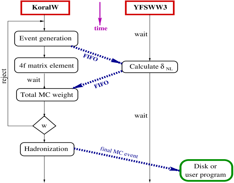
Figure 1: The time-flow chart for the present CMC KoralW$\&$YFSWW3. The line marked FIFO denotes the transfer of an event record from one process to another, using the named-pipes mechanism of UNIX.

As a result, KoralW can now, for example, perform the rejection and provide the constant-weight events with both the four-fermion background correction $\delta^{R}_{4f}$ and the ${\cal O}(\alpha)$ NL correction $\delta^{R}_{NL}$ to the $W$-pair production and decay process taken into account. Another application of such a scheme is the reweighting of events with both the four-fermion and ${\cal O}(\alpha)$ corrections included simultaneously in order to perform “Monte Carlo fits”.

To summarize it shortly: from the point of view of the user, the CMC program KoralW$\&$YFSWW3 works as a single Monte Carlo generator with all its normal features. This might be, to our knowledge, the first practical working implementation of such a scheme to the problem of the MC event generation in particle physics.

Remarkably, the efficiency of the CMC KoralW$\&$YFSWW3 in generating the constant-weight events according to the four-fermion background and the ${\cal O}(\alpha)$ NL corrected distributions is not bad. In principle one could worry that an additional YFSWW3 weight of the order of a few tens would translate into a similar increase of the maximal weight for rejection and, consequently, into a similar increase of the CPU time needed for the event generation. Surprisingly, however, this is not true! In the additive mode of combining KoralW and YFSWW3 the increase of the maximal weight that we recorded on the $2\times 10^{8}$ sample of variable-weight events was $1\to 5$, for example. Overweighted events were of two topologies. The first topology was strongly $WW$-like with multiple, i.e. at least triple, soft bremsstrahlung and led to overweights below 2 (in an extreme case with seven photons, we recorded an overweight of 4). The other topology was very far from $WW$-like (small values of the $W^{-}$, $W^{+}$ invariant masses) and gave the highest over-weights ($\sim 5$). In the latter cases the use of the on-shell ${\cal O}(\alpha)$ NL library is less justified anyway and these few events can simply be discarded, instead of increasing the maximal weight for the rejection. Why was the overweighting so small? Because in KoralW to cover the four-fermion-dominated configurations the maximal weights are adjusted higher than what is needed by the $WW$-like configurations. This extra safety margin turns out to be sufficient to absorb fluctuations of the additional $WW$-like ${\cal O}(\alpha)$ NL weights. The situation is different for the multiplicative prescription. Here, the big four-fermion weight is multiplied by the ${\cal O}(\alpha)$ NL correction, on occasion leading to overweights of the expected order of a few tens. This happens, typically, for a very hard bremsstrahlung photon, with energy of the order of 40 GeV. However, as we have explained earlier, the ${\cal O}(\alpha)$ correction for the configurations far away from being $WW$-like is less justified and the overweights provide merely another reason for using the additive scheme rather than the multiplicative one.

Let us add a few additional comments on the KoralW$\&$YFSWW3 CMC:

1. The corrections can be combined in an additive or multiplicative way, according to the discussion from the previous subsections.

2. One may also wonder about other possible source of efficiency loss caused by running two programs at the same time on a single processor. Our experience shows, however, that there is very little loss due to an alternate suspension of the programs, performed automatically by the operating system (in the UNIX kernel).

3. The big advantage of the FIFO special files is that they are in practice done by the operating system “in flight”, in virtual memory. Consequently, there is no need for a huge amount of disk space to store all the millions of generated events needed for generating the sample of the constant-weight events.

4. In order to introduce the “named pipes”, there is no need to modify in the FORTRAN source code of either of the programs. The only change is the replacement of regular input/output files by the special FIFO files, done at the level of the operating system and not in the FORTRAN source code. We give an example of such a procedure in the demo run of the CMC KoralW$\&$YFSWW3, which can be invoked through: make KandY (KandY stands for “K and Y”). It creates two special FIFO files 4vect.data.special and wtext.data.special that will serve for transmitting the four-momenta and the weights between the programs. These special FIFO files are then linked to the appropriate input/output file names for KoralW and YFSWW3 in their local working directories.

5. Finally, the two programs are executed with the common default data cards! They are modified later on by the user cards located in the local working directory.

The proposed scheme of CMC KoralW $\to$ YFSWW3 $\to$ KoralW is not the only possibility of realizing the four-fermion background and ${\cal O}(\alpha)$ NL corrected events. Alternatively, one can construct the CMC the other way around: YFSWW3 $\to$ KoralW $\to$ YFSWW3 (symbolically YFSWW3$\&$KoralW). In general, this direction has a serious drawback – the four-fermion correction weight from KoralW can be very high, especially for the final states with electrons, spoiling the convergence of the series. On the contrary, the YFSWW3 weight for the ${\cal O}(\alpha)$ NL correction is well behaved and for LEP2 energies it seems not to exceed a few tens. However, if the phase space for generation were restricted to $WW$-like configurations the situation would be reversed – the four-fermion correction weight would be smaller than the ${\cal O}(\alpha)$ NL one and the scheme YFSWW3$\&$KoralW would be a good choice.

We conclude this section with two technical remarks on the FIFO mechanism. They may prove useful in practical implementations of FIFOs.

1. The FIFO special files must be created (by the command “mkfifo file_name”) on a local disk of a computer on which the program will be executed. This means in particular that it cannot be created directly on the AFS file system or even on a mounted remote file system. The good location is, for example, the /tmp directory. After creation, however, the FIFO special file can be symbolically linked to any location in the mounted or AFS file systems. The FIFO special file itself requires only 4kB of disk space.

2. In certain configurations of the data transfer through named pipes, it may be at some point necessary to flush the output buffers of the programs. The syntax of the FORTRAN command for that operation is call flush(unit_number).

2.2.4 Possible future development

Our present modest application of the parallel processing to MC event generation is schematically depicted in Fig. 1. Note that on a dual-processor machine, at a certain moment KoralW is calculating the four-fermion matrix element while YFSWW3 is simultaneously calculating the electroweak ${\cal O}(\alpha$) corrections. In the present form, however, KoralW$\&$YFSWW3 does not really allow us to profit fully from running on the multiprocessor machine. It is mainly because the calculation of the ${\cal O}(\alpha$) NL correction takes on average longer than the calculation of the four-fermion correction; as a result the KoralW process is sometimes waiting for YFSWW3 before the final reprocessing of the event. Also hadronization by JETSET, which takes a substantial amount of CPU time and is independent from KoralW and YFSWW3, is not delegated to a separate process, but included as a part of KoralW.

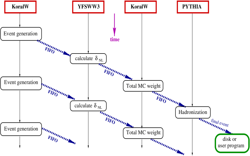
Figure 2: The time-flow chart for the possible future concurrent cascade-type arrangement of KoralW, YFSWW3 and a hadronization package such as PYTHIA.

In Fig. 2 we show another possible future concurrent arrangement, which would work more efficiently on the multiprocessor installation. Here, four independent processes work “in the cascade”, in such a way that when the last process (PYTHIA) finishes to hadronize an event, the first process may have already started to construct the next event. A similar solution was proposed in Ref. [35], however limited to a solution in which MC generators communicate through disk files (database). Of course, there are many other possible variants of such a scheme – the best one should be adapted to a particular MC generation problem and to available hardware.

The important advantage of such a concurrent arrangement is that it provides “encapsulation” for the “dusted deck programs”, without the need of laboriously translating them to object-oriented C++ or another OO programming language. It also allows an easy combination of programs written in different programming languages. This may prove to be in practice a rather effective solution, before eventual emergence of the next generation of event generators, written from scratch in the OO environment.

3 Numerical tests

Although the basic idea of reweighting MC events, produced either by the same MC event generator or the other one, is relatively simple, its actual implementation has to be tested very carefully. Such tests are the principal aim of the present section. We shall concentrate on the reweighting of MC events produced by KoralW using the correction weight produced by YFSWW3, that is on the “asymmetric” procedure $K+\delta Y$ described in Subsection 2.2.2. Before the programming tools for such a scenario can be fully trusted, we have to perform certain important introductory numerical tests:

(A)

We are going to check numerically that the common reference differential distributions $d\sigma^{R}$ generated by KoralW and YFSWW3 are the same.

(B)

For the distribution $d\sigma^{Test}=d\sigma^{{\cal O}(\alpha)+ISR_{23}+Cc}$ we are going to test the reweighting tools of KoralW and YFSWW3:

(B.1)

Self-test of YFSWW3: we shall compare results from the standard run of YFSWW3 and from the run $Y+\delta Y$ in which $d\sigma^{Test}$ is obtained by reweighting events generated according to $d\sigma^{R}$.

(B.2)

Calibration of $Y+\delta K$ using YFSWW3: we shall compare results of $Y+\delta K$ (in which events generated according to $d\sigma^{R}$ by KoralW are reweighted with the help of YFSWW3) with the direct results of YFSWW3 and with the results of the $Y+\delta Y$ scheme.

In both kinds of tests, numerical results for the cross sections and the key distributions, for instance the distributions of the $W$ mass, $W$ scattering angle and photon energy, should agree within statistical errors. We shall use the approximate version of the correcting weight ($\delta_{NL-}$ from YFSWW3). Test (B) will provide the measure of the quality of the approximation.

In all numerical tests in this section, the input parameter set-up and the definitions of event acceptances are that of Ref. [36], unless stated otherwise. For the convenience of the reader, let us recall briefly these acceptance conditions.

For the distributions we used the following cuts/acceptances:

1. We required that the polar angle of any charged final-state fermion with respect to the beams be $\theta_{f_{ch}}>10^{\circ}$.

2. All photons within a cone of $5^{\circ}$ around the beams were treated as invisible, i.e. they were disregarded in the calculation of any observable.

3. The invariant mass of a visible photon with each charged final-state fermion, $M_{f_{ch}}$, was calculated, and the minimum value $M^{min}_{f_{ch}}$ was found. If $M^{min}_{f_{ch}}<M_{rec}$ or if the photon energy $E_{\gamma}<1\,$GeV, the photon was combined with the corresponding fermion, i.e. the photon four-momentum was added to the fermion four-momentum and the photon was discarded. This was repeated for all visible photons.

   In our numerical tests we used two values of the recombination cut:

   $$M_{rec}=\left\{\begin{tabular}[]{l}\> 5\,{\rm GeV:} \hskip 28.45274pt {\rm CAL05},\\ 25\,{\rm GeV:} \hskip 28.45274pt {\rm CAL25}.\end{tabular}\right.$$

   Let us remark that we have changed here the labeling of these recombination cuts from the slightly misleading BARE and CALO names used in Ref. [36]. This change allows us to reserve the BARE name for a truly bare setup (without any recombination).

The integrated cross sections presented here were obtained without any cuts (labeled in the tables “NO CUTS”) or with the cut No. 1 from the above acceptance conditions (labeled in the tables “WITH CUTS”).

3.1 Integrated cross sections

NO CUTS
Description	Program	$\sigma^{\rm CC03}$[fb]	$\sigma^{R}$[fb]	${\bar{\delta}}^{\rm CC03}_{4f}[\%]$	$\bar{\delta}^{R}_{4f}[\%]$	$\bar{\delta}^{R}_{NL}[\%]$
	YFSWW3	$219.793\,(16)$	$204.198\,(09)$	—	—	$-1.92\,(4)$
$\nu_{\mu}\mu^{+}\tau^{-}\bar{\nu}_{\tau}$	KoralW	$219.766\,(26)$	$204.178\,(21)$	$0.041$	$0.044$	—
200 GeV	(Y$-$K)/Y	$0.01\,(1)\%$	$0.01\,(1)\%$	—	—	—
	YFSWW3	$659.69\,(5)$	$635.81\,(3)$	—	—	$-1.99\,(4)$
$u\bar{d}\mu^{-}\bar{\nu}_{\mu}$	KoralW	$659.59\,(8)$	$635.69\,(7)$	$0.073$	$0.073$	—
200 GeV	(Y$-$K)/Y	$0.02\,(1)\%$	$0.02\,(1)\%$	—	—	—
	YFSWW3	$1978.37\,(14)$	$1978.00\,(09)$	—	—	$-2.06\,(4)$
$u\bar{d}s\bar{c}$	KoralW	$1977.89\,(25)$	$1977.64\,(21)$	$0.060$	$0.061$	—
200 GeV	(Y$-$K)/Y	$0.02\,(1)\%$	$0.02\,(1)\%$	—	—	—
WITH CUTS
	YFSWW3	$210.938\,(16)$	$196.205\,(09)$	—	—	$-1.93\,(4)$
$\nu_{\mu}\mu^{+}\tau^{-}\bar{\nu}_{\tau}$	KoralW	$210.911\,(26)$	$196.174\,(21)$	$0.041$	$0.044$	—
200 GeV	(Y$-$K)/Y	$0.01\,(1)\%$	$0.02\,(1)\%$	—	—	—
	YFSWW3	$627.22\,(5)$	$605.18\,(3)$	—	—	$-2.00\,(4)$
$u\bar{d}\mu^{-}\bar{\nu}_{\mu}$	KoralW	$627.13\,(8)$	$605.03\,(7)$	$0.074$	$0.074$	—
200 GeV	(Y$-$K)/Y	$0.01\,(1)\%$	$0.02\,(1)\%$	—	—	—
	YFSWW3	$1863.60\,(15)$	$1865.00\,(09)$	—	—	$-2.06\,(4)$
$u\bar{d}s\bar{c}$	KoralW	$1863.07\,(25)$	$1864.62\,(21)$	$0.065$	$0.064$	—
200 GeV	(Y$-$K)/Y	$0.03\,(2)\%$	$0.02\,(1)\%$	—	—	—

Table 1: The numerical check of equality of the integrated reference cross sections $\sigma^{R}$ from YFSWW3 and KoralW. We also include $\sigma^{\rm CC03}$ in which the ISR is switched off (CC03 Born). All results are at $\sqrt{s}=200$ GeV, with and without cuts. Corrections due to the background diagrams and the missing ${\cal O}(\alpha$) are also indicated; see the text for more explanation. The statistical errors corresponding to the last digits are indicated in parentheses.

The first test of type (A) is presented in Table 1, where we check whether the integrated reference cross section $\sigma^{R}$ defined in the previous section is numerically the same when calculated by KoralW and YFSWW3. It is done for three examples of the CC11 class process (see Ref. [36] for its definition) at the center-of-mass system (CMS) energy $\sqrt{s}=200$ GeV. In addition to the standard $\sigma^{R}$ of the previous section, we also show results for $\sigma^{\rm CC03}$, which is a variant of $\sigma^{R}$ in which the ISR is switched off. As already indicated, it is the so-called CC03 process (in the ’t Hooft–Feynman gauge). As we see in Table 1, the relative differences of the reference cross sections $\sigma^{R}$ and $\sigma^{\rm CC03}$ of YFSWW3 and KoralW are below $3\times 10^{-4}$. This test indicates that the reference differential cross section $d\sigma^{R}$ is implemented correctly through the corresponding MC weight in both KoralW and YFSWW3. In Table 1, we also indicate the size of the correction $\bar{\delta}^{R}_{4f}$ due to the background diagrams and $\bar{\delta}^{R}_{NL}$ due to the missing ${\cal O}(\alpha$), which are defined as follows:

$$\bar{\delta}^{R}_{4f} =\frac{\sigma_{K}^{4f+{\rm ISR_{123}+Cc}}-\sigma^{\rm CC03+ISR_{123}+Cc}}{\sigma^{\rm CC03}},$$ (25)

$$\bar{\delta}^{\rm CC03}_{4f} =\frac{\sigma_{K}^{4f}-\sigma^{\rm CC03}}{\sigma^{\rm CC03}},$$

$$\bar{\delta}^{R}_{NL} =\frac{\sigma_{Y_{a}}^{\rm{\cal O}(\alpha)+ISR_{23}+Cc}-\sigma^{\rm CC03+ISR_{123}+Cc}}{\sigma^{\rm CC03}}.$$

Note that in Table 1 the final-state QCD correction is excluded from $\bar{\delta}^{R}_{4f}$ (i.e. $\bar{\delta}^{R}_{4f}$ is divided by $(1+\alpha_{S}/\pi)$). Note also that the Coulomb correction is taken here without screening.

NO CUTS
Description	Program	$\sigma^{\rm CC03}$[fb]	$\sigma_{R}$[fb]	$\bar{\delta}^{\rm CC03}_{4f}[\%]$	$\bar{\delta}^{R}_{4f}[\%]$	$\bar{\delta}^{R}_{NL}[\%]$
	YFSWW3	$156.670\,(16)$	$122.832\,(08)$	—	—	$-1.41\,(4)$
$u\bar{d}\mu^{-}\bar{\nu}_{\mu}$	KoralW	$156.601\,(24)$	$122.836\,(11)$	$0.29$	$0.25$	—
161 GeV	(Y$-$K)/Y	$0.04\,(2)\%$	$0.00\,(1)\%$	—	—	—
WITH CUTS
	YFSWW3	$151.158\,(16)$	$118.482\,(08)$	—	—	$-1.41\,(4)$
$u\bar{d}\mu^{-}\bar{\nu}_{\mu}$	KoralW	$151.089\,(24)$	$118.485\,(11)$	$0.29$	$0.25$	—
161 GeV	(Y$-$K)/Y	$0.05\,(2)\%$	$0.00\,(1)\%$	—	—	—
NO CUTS
	YFSWW3	$261.368\,(23)$	$292.029\,(18)$	—	—	$-4.95\,(4)$
$u\bar{d}\mu^{-}\bar{\nu}_{\mu}$	KoralW	$261.348\,(17)$	$291.979\,(19)$	$-0.51$	$-0.51$	—
500 GeV	(Y$-$K)/Y	$0.01\,(1)\%$	$0.02\,(1)\%$	—	—	—
YFSWW3-like	KoralW	$261.348\,(17)$	$291.980\,(22)$	$-0.51$	$-0.51$	—
extrapol.	(Y$-$K)/Y	$0.01\,(1)\%$	$0.02\,(1)\%$	—	—	—
WITH CUTS
	YFSWW3	$181.505\,(22)$	$209.449\,(17)$	—	—	$-6.34\,(4)$
$u\bar{d}\mu^{-}\bar{\nu}_{\mu}$	KoralW	$181.480\,(17)$	$209.592\,(18)$	$-0.69$	$-0.69$	—
500 GeV	(Y$-$K)/Y	$0.01\,(1)\%$	$-0.07\,(1)\%$	—	—	—
YFSWW3-like	KoralW	$181.480\,(17)$	$209.426\,(21)$	$-0.69$	$-0.69$	—
extrapol.	(Y$-$K)/Y	$0.01\,(1)\%$	$0.01\,(1)\%$	—	—	—

Table 2: The numerical check of equality of the integrated reference cross sections $\sigma^{R}$ from YFSWW3 and KoralW, as in Table 1, but for two other energies: 161 GeV and 500 GeV.

In Table 2, we present the analogous (A)-type test for the integrated cross sections as in Table 1 but for two other CMS energies: close to the $WW$-threshold, 161 GeV, and at 500 GeV, within the range of the future Linear Collider. As we see, the result of the test is again positive. The integrated reference cross section $\sigma^{R}$ is again the same from both YFSWW3 and KoralW to within $5\times 10^{-4}$. In Table 2, we also show the effect of switching from the extrapolation/reduction procedure of KoralW to that of YFSWW3 (which is the source of the largest discrepancy of $-0.07\%$). One can verify that the size of this effect is at the sub-per mille level and appears only in the case with imposed cuts. For the case without any cuts there is no difference in the total cross section, as expected. Note that Table 2 shows the case of $\sqrt{s}=500$ GeV. At $\sqrt{s}=200$ GeV, there is no difference between these two extrapolation procedures.

Type of calculation		NO CUTS		WITH CUTS
MC	Formula	$\sigma_{i}$ [fb]	$\frac{\sigma_{i}}{\sigma_{1}}-1$	$\sigma_{i}$ [fb]	$\frac{\sigma_{i}}{\sigma_{1}}-1$
$Y$	$\sigma_{1}=\sigma_{Y_{a}}^{{\cal O}(\alpha)+ISR_{23}+Cc}$	$623.07\,(14)$	—	$593.03\,(15)$	—
$Y+\delta Y$	$\sigma_{2}=\int d\sigma_{Y_{a}}^{R}[1+\delta^{R}_{NL-}]_{Y}$	$622.59\,(14)$	$-0.08(3)\%$	$592.57\,(14)$	$-0.08(3)\%$
$K+\delta Y$	$\sigma_{3}=\int d\sigma_{K}^{R}[1+\delta^{R}_{NL-}]_{Y}$	$622.68\,(17)$	$-0.06(4)\%$	$592.58\,(17)$	$-0.06(4)\%$
$K+\delta Y$	$\sigma_{4}=\int d\sigma_{K}\left[1+\frac{\delta^{R}_{NL-}}{1+\delta^{R}_{4f}}\right]$	$623.24\,(6)$	$+0.03(2)\%$	$593.14\,(6)$	$+0.02(3)\%$
$K+\delta Y$	$\sigma_{5}=\sigma_{3}$($4f$ presampler)	$622.74\,(6)$	$-0.05(2)\%$	$592.66\,(6)$	$-0.06(3)\%$

Table 3: The self-test of YFSWW3 ($Y+\delta Y$) and the test of CMC KoralW$\&$YFSWW3 ($K+\delta Y$) for the ${\cal O}(\alpha$)-corrected integrated cross section $\sigma^{{\cal O}(\alpha)+ISR_{23}+Cc}$ (no background diagrams). All results are at $\sqrt{s}=200$ GeV, for the $u\bar{d}\mu^{-}\bar{\nu}_{\mu}$ final state, with and without cuts. The statistical errors corresponding to the last digits are indicated in parentheses.

In Table 3 (test (B)), we show in the first line the standard “best” result of YFSWW3. In the second line we present the self-test of YFSWW3 of the type $Y+\delta Y$ in which events are primarily generated with YFSWW3 according to the reference distribution $d\sigma^{R}=d\sigma^{CC03+ISR_{123}+Cc}$ and are later reweighted using the weight $[1+\delta^{R}_{NL-}]_{Y}$ calculated also by YFSWW3. In the third line we show the test of the CMC KoralW$\&$YFSWW3 of the type $K+\delta Y$, in which events are generated using KoralW according to $d\sigma^{R}$ and are reweighted using the same weight $[1+\delta^{R}_{NL-}]_{Y}$ provided by YFSWW3. The $\sigma_{2}$ and $\sigma_{3}$ represent the same quantity generated in two different ways, and indeed the numerical agreement between them is well within the statistical errors. The agreement of the latter two results with the first one is within $0.08\%$. It is sufficient for the purpose of LEP2. Note that we do not expect perfect agreement, owing to the use of the approximate $\delta^{R}_{NL-}$. The above discrepancy is also much smaller than the size of the NL correction itself, which is often up to $2\%$. In the fourth line we show the result of the CMC KoralW$\&$YFSWW3 in the full operational mode. Since the four-fermion correction is rather small we have checked, using differences of the MC weights, that the four-fermion correction contribution in $\sigma_{4}$ is $0.4985(17)\,$fb, that is $0.0728(2)\%$ in units of the CC03 cross section (adjusting also for the QCD factor $(1+\alpha_{S}/\pi)$) for the “No-Cuts” case, and $0.4822(17)\,$fb, i.e. $0.0741(3)\%$ for the “With-Cuts” case. This is fully compatible with the results shown in Table 1. Finally, in the fifth line we show again calculation of the cross section equal to $\sigma_{3}$, obtained, however, as a by-product of the previous CMC KoralW$\&$YFSWW3 run in the full operational mode, with different arrangement of the MC weights. As compared with the original $\sigma_{3}$ calculation, KoralW is now run in the CCall mode instead of the CC03. The equality $\sigma_{3}=\sigma_{5}$ (within the statistical errors), provides yet another consistency check of the CMC KoralW$\&$YFSWW3.

3.2 One-dimensional distributions

The example of a purely technical test is also presented in Fig. 5, where we check that the $d\sigma^{R}$ distribution of the polar angle of the $W$ and of the photon angle with respect to the final charged fermion is the same, after adjusting the reduction/extrapolation procedure to be the same in KoralW as in YFSWW3, while it was not the same for the original reduction/extrapolation procedure of KoralW version 1.41.

Another technical test is presented in Figs. 6 and 7 (test (A)) where we check, for various distributions, that the reference distribution $d\sigma^{R}$ is identically implemented in KoralW and YFSWW3. The distributions of the $W$ mass and angle, of the photon energy and angle are the same within the statistical errors. We conclude that $d\sigma^{R}$ is implemented correctly, at the precision level relevant to LEP2.

Finally, in Figs. 8 and 9, we calibrate the CMC KoralW$\&$YFSWW3 using YFSWW3 for the distribution $d\sigma^{\rm{\cal O}(\alpha)+ISR_{23}+Cc}$ (test (B)). Again, for the distributions of the $W$ mass and angle, of the photon energy and angle, we see the satisfactory agreement between the results of the CMC KoralW$\&$YFSWW3 and of YFSWW3, with the exception of the angular distribution of the hardest photon, where a small deviation shows up for large angles. We attribute it to the use of the approximate character of $\delta^{R}_{NL-}$ provided by YFSWW3. In the last two figures, we also indicate the size of the NL and four-fermion corrections. For a more exhaustive discussion of the complete “best” results of the CMC KoralW$\&$YFSWW3 we refer the reader to other works [23].

4 Details of modifications of KoralW version 1.51

In this section we describe in detail all the modifications introduced in the version 1.51 of KoralW with respect to the previous version 1.41.

In the first subsection we present the changes that allow the use of KoralW together with YFSWW3 in the form of Concurrent Monte Carlo KoralW$\&$YFSWW3. The key modification necessary for this scheme is the option of reprocessing by KoralW the events stored on some external device, generated earlier by KoralW or YFSWW3. In addition, a new optional “extrapolation procedure”, as in YFSWW3, and a new, screened, Coulomb correction have been implemented in KoralW to ensure the full compatibility of KoralW with YFSWW3, whereas a new optional normalization scheme allows for cross-checks with other programs, such as RacoonWW for example.

In the next subsection we will describe modifications that will be helpful in the application of KoralW to study the background to the two-fermion processes due to the emission of a secondary fermion pair. The idea is to calculate separately the contribution from the real fermion-pair emission in the complete phase space and the virtual corrections; see [30] for more details. The corresponding virtual pair contribution should be calculated by the $\cal KK$ Monte Carlo program [37] and the cancellation between the leading real and virtual logarithms is done numerically. The use of the MC program for calculating these corrections may be an interesting alternative to the semi-analytical approach. More information on this approach to the fermion-pair corrections in the two-fermion processes can be found in [30]. The presented modifications of KoralW provide a number of approximate matrix elements (ISNS, FSNS, etc.) and a new “extrapolation procedure” oriented toward the $t$-channel-dominated photonic radiation.

Finally, in the last subsection we shall describe “miscellaneous” modifications not related directly to any of the above subjects.

4.1 Modifications related to $W$-pair processes and communication with YFSWW3

4.1.1 Switches activating reading and writing events

We have added switches to activate and steer the process of reading events in the form of a list of four-vectors from the external file, instead of generating them. The four-vectors must be located in the file 4vect.data.in and the exact format is specified in the subroutine reader2 in korww/karludw.f. The relevant input parameter i_disk is set in the standard way, as other input parameters; see Table 5. It may be set as follows: i_disk=0 (default), standard MC generation of four-vectors (no reading events); i_disk=1, internal tests on the four-fermion presampler; i_disk=2,3,4, new settings for reading the four-vectors for FIFO. When using FIFO the user of the program should adjust the style formats for the reading of four-momenta from the storage file by setting the values 2, 3 or 4 to the variable i_disk. Let us describe this organization in more detail:

i_disk=0:

standard MC generation of four-vectors (no reading).

i_disk=1:

internal tests of the four-fermion presampler (special tests).

i_disk=2 (reading from the disk file):

an event is read from an external ASCII file in a format close to the PDG common block; four-momenta of all four final fermions, the number of photons and their four-momenta (if present) – let us call the above a “PDG event record”; for the actual formats see the subroutine reader2.

i_disk=3 (for FIFO):

in this case a normal event starts with a line with any single character (character*1) other than “E” followed by a “PDG event record” in the format of the i_disk=2 case; if the first line contains the character “E” then the reading program exits immediately.

i_disk=4 (for FIFO):

in this case a normal event starts with a line with any single character (character*1) other than “R” and “E” followed by the “PDG event record” and followed by the MC weight; alternatively, the event may start with the marker “R” in the first line, followed by the (almost) empty PDG record and the weight; finally (alternatively), the line with marker “E” terminates the reading process immediately.

There is a corresponding switch i_writ_4v=2,3,4 which, upon activation, causes KoralW to write the file 4vect.data.out in the formats corresponding exactly to the ones specified for the above settings of i_disk.

It must be kept in mind that in the mode i_disk=2,3,4, KoralW will not calculate certain parts of the differential distributions $d\sigma_{K}$. In this case only the ratios of the four-fermion matrix element weights (wtset(1-4,6-9)) are meaningful; for example, we have wtset(i_prwt)/wtset(10-i_prwt)$=1+\delta^{R}_{4f}$, see eq. (14).

Note that i_disk=2,3,4 works for the ISR as well as for the CC03. An inclusive mixture of the final states with different flavor composition is also allowed.

It is also sometimes useful to switch off the printouts for weights over wtmax by setting i_prnt=0 while reading four-vectors from the file (as wtmax makes no sense in this context).

4.1.2 Switches activating reading and writing weights

There are two additional keys, which are steering the process of writing and reading Monte Carlo weights from the external files i_writ_wt and i_read_wt. The i_writ_wt key activates writing weights into the file wtext.data.out in the subroutine writer_wt in korww/karludw.f:

i_writ_wt=1:

Only one external weight wtext = wtset(i_prwt)/wtset(10-i_prwt) is written. The input variable i_prwt (see Table 5) defines the perturbative order of the ISR for the best (principal) weight.

i_writ_wt=3:

The first nine entries from the wtset matrix are written.

The i_read_wt key has a twofold function: it controls reading weights from the external device (from the file wtext.data.in) and it optionally activates special tests of this procedure (of no interest for the user). For positive values, various modes of reading weights from the file are invoked:

i_read_wt=1:

One external weight wtEXT is read and combined in an additive way with the entries 1–9 of the wtset matrix:
wtset(i)=wtset(i)+wtset(10-i_prwt)*(wtEXT - 1).

i_read_wt=2:

One external weight wtEXT is read and combined in a multiplicative way with the entries 1–9 of the wtset matrix: wtset(i)=wtset(i)*wtEXT.

i_read_wt=3:

Nine weights are read and stored as entries 1–9 of the wtset matrix, overwriting the old values.

i_read_wt=4:

Nine weights are read and stored as entries 91–99 of the wtset matrix.

For negative values of i_read_wt certain tests are performed on the weights from the disk.

i_read_wt=–3:

The wtset entries 1–9 are read and compared with the ones calculated directly by KoralW.

i_read_wt=–2:

A single wtEXT is read and compared with the four-fermion matrix element calculated directly by KoralW (this is useful for checking the conventions of the matrix element).

i_read_wt=–1:

A single wtEXT is read and compared with the CC03 matrix element calculated directly by KoralW (this is useful for checking the conventions of the matrix element).

User must be aware of the high sensitivity of the four-fermion matrix element with respect to small changes of the four-vectors. For example, in order to reproduce the original wtset weights when recalculated by KoralW in the i_disk > 1 mode, an additional kinematical tune-up (the Lorentz boost from the LAB frame to the effective CMS_eff) has been permanently introduced in version 1.51 (marked with the special string <<<< tune-up >>>> in the source file karlud.f). If four-momenta are generated by YFSWW3, then KeyISR=2 should be chosen (see below for more details on the new meaning of KeyISR=2) to ensure the compatibility of the ISR “extrapolation procedures”.

4.1.3 New MC weights related to CC03

Already in the previous version, 1.42, of KoralW the CC03 matrix element was always calculated, even in the CCall mode (Key4f=1). In the present version, the MC weight corresponding of the CC03 matrix element is now always provided (also for Key4f=1) by KoralW as wtset(10-i), where i=4 corresponds to the standard (best) ${\cal O}(\alpha^{3}$) exponentiated LL variant of the ISR distribution ($d\sigma^{R}$). The other variants ${\cal O}(\alpha^{i-1}$) $i=1,2,3$ are also provided for each event. For Key4f=1 the other wtset(i) provide, as before, the values of the MC weights corresponding to the CCall matrix element. The above arrangement provides an event-per-event access to the difference CCall$-$CC03:

$${\tt wtdiff=wtcrud*(wtset(i)-wtset(10-i))},$$ (26)

as well as the elements for the construction of the four-fermion correction weight

$$[1+\delta_{4f}^{R}]_{K}=\frac{d\sigma_{K}^{4f+ISR_{1...(i-1)}+Cc}}{d\sigma^{R}}=\frac{|M^{4f}(\{p,q\}^{{\cal R}})|^{2}}{|M^{\rm CC03}(\{p,q\}^{{\cal R}})|^{2}}=\frac{\tt wtset(i)}{\tt wtset(10-i)},$$ (27)

see Eqs. (14) and (23), necessary for reweighting the YFSWW3 events.

4.1.4 New extrapolation/reduction procedure

The next modification concerns the “extrapolation procedure”, i.e. the calculation of the Born-level four-fermion matrix element in the presence of multiple photons. The four-fermion matrix element, defined for points from the four-body phase space, has to be extrapolated to points from the multibody phase space. In other words, the multibody phase space has to be projected onto the four-body phase space. There is a freedom in defining this procedure and the default ones in KoralW and YFSWW3 differ by a finite rotation of the effective CMS frame of the final-state fermions with respect to the laboratory frame, leading to differences in some photonic distributions (but not in the total cross-section!). Therefore, the new procedure we introduced in KoralW is identical to that in YFSWW3. It is accessible under the KeyISR=2 setting in the input cards. Note that the physical origin of this freedom is the lack of the complete $4f+n\gamma$ matrix elements. They are approximated correctly in both the soft and collinear limits (up to $n=3$) but miss some non-leading-logarithmic corrections for transverse photons, responsible for this ambiguity.

4.1.5 Screened Coulomb correction

The screened Coulomb correction as proposed in Ref. [33] has been added. It can be activated by setting the KeyCul input parameter to KeyCul=2. This ansatz is an efficient approximation of the non-factorizable corrections. It is also helpful for comparisons, with YFSWW3, with the screened Coulomb correction as the default option.

4.1.6 New meanings of KeyBra switch

The KeyBra switch has changed some of its meaning. Namely, the setting KeyBra=1 has been modified. In version 1.42 it took the arbitrary values of $W$ decay branching ratios from the input while fixing the value of $\alpha_{S}$ at $0.12$ and recalculating the $W$ width $\Gamma_{W}=3/(2\sqrt{2}\pi)M_{W}^{3}G_{\mu}(1+(2/3)(\alpha_{S}/\pi))$. Such an input set-up could have led to inconsistency if the branching ratios had been changed from the supplied default values.

The modified setting KeyBra=1 allows for arbitrary $W$ decay branching ratios as well as $\alpha_{S}$ and $\Gamma_{W}$, taken without any consistency checks and modifications from the input cards. This option changes also the way the CC03 matrix element is normalized. The new normalization of the Born CC03 matrix element in the KeyBra=1 mode is the following. Instead of the Br($W\to e\nu_{e}$) from the input, the Standard Model value Br${}_{el}={\alpha_{W}M_{W}}/(12\sin^{2}\theta_{W}\Gamma_{W})$ is taken, and the normalization of the decay channel $(i,j)$ is set by the factor $\hbox{Br}_{i}\hbox{Br}_{j}/\hbox{Br}_{el}^{2}$ with respect to the ($e\bar{\nu}_{e},\nu_{e}\bar{e}$) decay channel.

These changes were necessary in order to allow for running KoralW with the input parameters as defined by RacoonWW in its comparisons with YFSWW3 in [36]. In this way, KoralW and the CMC KoralW$\&$YFSWW3 can be directly used for the comparisons with RacoonWW.

The “old” setting KeyBra=1 of the version 1.42 has been preserved under the new setting KeyBra=3 with the only change that now the $W$ branching ratios are not taken from the input but are “hardwired” into the source code (to their default values of the version 1.42) enforcing consistency with the $W$ width and $\alpha_{S}$, which are also set in the program.

KeyBra=2 remains unchanged.

4.1.7 New meanings of the KeyMix switch

The default value of the KeyMix parameter has been changed from KeyMix=0 to KeyMix=1. This key chooses the electroweak “Input Parameter Scheme”, and the accessible settings are KeyMix=0: “LEP2 Workshop 1995” scheme and KeyMix=1: $G_{\mu}$-scheme. In the previous versions we recommended the scheme KeyMix=0, worked out throughout the 1995 LEP2 Workshop. However in YFSWW3 only the standard $G_{\mu}$-scheme is available for the ${\cal O}(\alpha)$ NL corrections. Therefore, in order to make the two programs compatible, we changed the default scheme to $G_{\mu}$ in KoralW as well. It must be stressed that the Born level difference between the “LEP2”-scheme and $G_{\mu}$-scheme is well below the quoted 2% physical precision of KoralW, and both choices are equally legitimate. This difference itself is due to the ${\cal O}(\alpha)$ NL corrections to the Born process missing in KoralW. Therefore, when the ${\cal O}(\alpha)$ NL corrections are calculated with the YFSWW3, the problem is solved – now the difference between any two schemes is due to the second-order corrections and can be neglected.

4.2 Modifications related to two-fermion and $t$-channel-dominated processes

4.2.1 New i_sw4f switch for selecting subgroups of Feynman graphs in the matrix element

The option of downgrading the complete four-fermion matrix element to certain sub-classes of graphs has been implemented for some final states. It can be activated with the input parameter i_sw4f. It has been installed with an eye toward applications of KoralW in the calculation of the background to the two-fermion processes due to the emission of an additional fermion pair. Therefore the implemented options have been motivated by the options available in the Gentle program [38]. Denoting initial states non-singlets as ISNS and final-state non-singlets as FSNS (see also ref. [36]) the following options are available:

i_sw4f=–1:

all approximations set in the data parameter /isw4f/ in amp4f.f; transmitted out with the wt4f(9) weight,

i_sw4f=0:

the CC03 approximation,

i_sw4f=1:

the complete four-fermion (default),

i_sw4f=2:

the ISNS_γ+Z $\tau^{+}\tau^{-}$ pair emission in the $e^{+}e^{-}\to\mu^{+}\mu^{-}$ process,

i_sw4f=3:

the FSNS_γ+Z $\tau^{+}\tau^{-}$ pair emission in the $e^{+}e^{-}\to\mu^{+}\mu^{-}$ process,

i_sw4f=4:

the ISNS_γ +FSNS_γ $\tau^{+}\tau^{-}$ or $e^{+}e^{-}$ pair emission in the $e^{+}e^{-}\to\mu^{+}\mu^{-}$ process,

i_sw4f=5:

the ISNS_γ $\tau^{+}\tau^{-}$ or $e^{+}e^{-}$ pair emission in the $e^{+}e^{-}\to\mu^{+}\mu^{-}$ process,

i_sw4f=6:

the FSNS_γ+Z $\mu^{+}\mu^{-}$ pair emission in the $e^{+}e^{-}\to\tau^{+}\tau^{-}$ process.

Further approximations can be added in the subroutine selgrf located in the file
grc4f_init/selgrf.f. The ibackgr variable denotes the value of i_sw4f, whereas nthprc is the decay channel number as defined in the amp4f routine (with the variable idef).

4.2.2 New reduction/extrapolation procedure for $t$-channel processes

Another “extrapolation procedure” (accessible with the KeyISR=3 setting) has been implemented in KoralW in order to improve on photonic emission in the case of the $t$-channel-dominated processes. The standard option of KoralW (i.e. KeyISR=1) for matching the ISR QED bremsstrahlung generation with the generation of the Born-level hard process is designed in a way that assumes that the four-fermion process always involves a substantial contribution from the $s$-channel interactions. That is the preferred approach in the case of the CC03 $W$-pair production and decay. However, in such cases as the generation of the fermion-pair corrections to the two-fermion final states, it is no longer the optimal one. Of course, in such configurations the whole assumption of the separate treatment of the QED photonic ISR bremsstrahlung and the fermion-pair emission is not the best one, even for the lowest-order approximation. The standard KoralW solution is however much worse, since it breaks the principle of the leading-log treatment. This leads to some pathologies as described in the program documentation, which consist of uncontrolled wash-out of the fermions originally generated close to the beam pipe toward larger angles and eventually down to the acceptance region.

Fortunately this inconsistency is easy to fix, by following the logic of the LL approximation in which the photon and fermion-pair emissions should not affect each other. This means that the bremsstrahlung should not modify the numerical value of the small $t$-channel transfers with which the four-fermion process matrix elements vary a lot.

The modification for the algorithm is localized in the subroutine from_cms_eff in the file karludw.f only. The kinematical transformation between the laboratory system and the four-fermion rest frame CMS_eff must depend not only on the momenta of the ISR photons but also on the final-state fermions. The freedom of rotating the effective CMS_eff frame of the final-state fermions with respect to the laboratory frame is used to ensure that the smallest scalar product of all eight products built out of one of the effective beams (in CMS_eff) and one of the final state four-momenta will be identical to the same product built out of the respective laboratory-frame four-momenta for the same beam and the final-state fermion.

4.3 Miscellaneous modifications

1. The semi-analytical part (KorWan) now supports a non-running $W$ width as well as the running one, i.e. the key KeyWu is now fully functional in semi-analytical calculations.

2. Automatic resetting of the low-level cuts to zero in the mode with the CC03 matrix element has been disabled. Now the cuts must be set in the input cards for both CC03 and four-fermion modes in an identical way.

3. The convention of writing four-momenta of the MIX-type CKM-suppressed final states ($d\bar{d}c\bar{c}$, $u\bar{u}s\bar{s}$, $u\bar{u}b\bar{b}$, $c\bar{c}b\bar{b}$) in the common blocks momdec and cms_eff_momdec has been unified in both the CC03 and four-fermion modes to the four-fermion convention (as given above in parentheses). This has been done in order to define uniquely the form of the input in the case of reading the four-momenta from the external file. The way the Lund common block is filled and hadronization is done for these states has not been changed, i.e. it is performed as $WW$ in the CC03 mode and as $ZZ$ in the four-fermion mode. This change removes the inconsistency of notation present in version 1.42.

4. Some of the dip-switches have been replaced by the input parameters and some new parameters have been added. See the Appendix for the complete list of the new input parameters in the data_DEFAULTS file.

5. The PHOTOS package [32] was updated with the new version, better adjusted to the present software requirements (Linux, HEPEVT of the non-standard dimensionality, etc.). The functionality of the program was not changed, except for the removal of the security check on photon emission from light quarks. Such an option is often in use for some $W$-pair studies, so even though from the physics point of view it is, as yet, of not much interest, we leave it here to enable tests/comparisons with other calculations. The radiation from both leptons and quarks is activated by the new setting ifphot=2 in the input parameters. The old ifphot=1 setting has not changed its meaning of the photon emission from leptons only. The appropriate warning message is printed by the version of PHOTOS included here.

   Note also that in the distribution version of TAUOLA the parameters in the $\tau$ decay modes are not adjusted to the recent experimental data. We recommend the user to replace this version of TAUOLA [39, 40] with the one accepted within her/his own collaboration. The technical update explained in Refs. [41, 42] will resolve this inconvenience in the future releases of the program.

5 Installation of KoralW version 1.51

The version 1.51 of KoralW is distributed as a stand-alone package as well as in the form of an update to the old version 1.42.3.

5.1 Stand-alone version

If one plans to use KoralW together with YFSWW3, the following steps should be observed:

• The main directory of the YFSWW3 program should be placed next to the KoralW main directory. (That means YFSWW3 should be visible from the KoralW main directory as ../yfsww3-1.16-export.)

• Next, one should descend into the directory demo.yfsww of KoralW and execute the make yfsww3-install command to perform the installation of the demo.koralw subdirectory in the YFSWW3 main directory. The name of the YFSWW3 directory can be specified in the makefile file in the demo.yfsww directory; the default name is yfsww3-1.16-export. This installation (make yfsww3-install) will be automatically performed when a demo run of KoralW$\&$YFSWW3 is invoked by make KandY or make XKandY.

• It may sometimes be necessary to set appropriate compiler flags, dependent on the operating system (the default is Linux RedHat versions 6.x and 7.x). To do this one must go to the main KoralW directory, set all relevant options in the makefile file in the first place and then execute the command make makfil. A similar operation may also be needed for the YFSWW3 program.

• At this moment the program is ready to use. One can descend again to the demo.yfsww directory and perform various tests.

5.2 Update of the old version

The patch source code is located in the koralw-1.51.x-export/demo.yfsww directory. To perform the update one should follow the following steps:

• Extract the directory demo.yfsww from the distribution version of KoralW 1.51 and move it to the main directory of KoralW 1.42.3, i.e. to koralw-1.42.3-export.

• If one plans to use KoralW together with YFSWW3, the main directory of the YFSWW3 source code (at present yfsww3-1.16-export) should be placed next to the directory koralw-1.42.3-export.

• After descending into the directory demo.yfsww one should execute the command make install to perform the actual installation. Upon installation, some of the original files of KoralW will be modified and, optionally, a new directory demo.koralw will be created in the yfsww3-1.16-export directory (the name of the YFSWW3 directory can be changed in the makefile file in demo.yfsww directory, the default is yfsww3-1.16-export). One can undo the changes by the make uninstall command.

• After installation, it is usually necessary to set appropriate compiler flags, dependent on the operating system. To do this one must go up to the main KoralW directory, set the options in the makefile file and execute the make makfil command. A similar operation may also be needed for the YFSWW3 source code.

• At this moment the source code is ready to compile and execute. One can descend again to the demo.yfsww directory and perform various tests.

5.3 Summary of the make commands relevant to the installation

In this subsection we summarize the options, available in the master makefile in the demo.yfsww directory, which are relevant to the installation.

5.3.1 Stand-alone version

• make yfsww3-install – installs the demo.koralw directory in the YFSWW3 main directory, necessary for the CMC KoralW$\&$YFSWW3

5.3.2 Update of the old version

• make install – creates the version 1.51 of KoralW out of the version 1.42.3

• make update – copies any changes in the source directory src into the KoralW-1.51 source code (useful for adding corrections)

• make uninstall – recovers the original KoralW version 1.42.3

6 Organization of the source code

The copy of FORTRAN files modified in the version 1.51 along with the tests specific to the $W$-physics are located in the single directory demo.yfsww. In this directory there are the demo program used for all the demo runs and the master makefile that defines the demo runs. The source code FORTRAN files of the version 1.51 are located in the demo.yfsww/src subdirectory. If the installation is performed in the form of an update – these files will replace the corresponding files of KoralW 1.42.3. Input/output files for tests are stored in a working directory (demo.yfsww/work). In the following we shall briefly describe some of the files in the demo.yfsww subdirectory.

• KWyfsww.f is the main program for tests. It does all the bookkeeping of cross-sections and histograms. The actual job is done by two subroutines: Prod1 for the Born-level comparisons and Prod3 for the ISR comparisons. Both routines use the set of cuts used in the comparisons between YFSWW3 and RacoonWW in [36] and plot several distributions for both the CCall cross-sections and the CCall$-$CC03 difference.

• makefile is the master makefile for the installation as well as for the tests.

• user_selecto.f – a dummy file for setting low-level cuts, no pre-cuts are set here.

• Subdirectory work
  In this subdirectory all the input files for the demo programs can be found and the output files are generated. For the exact assignment of the files to specific demo runs, we refer to the makefile file. Another three auxiliary files, iniseed with a seed for the random-number generator and the semaphore and semaphore.START flag-files for restarting the generation from a given event or to start from scratch, are also located there.

• Subdirectory work.tmp
  Some of the tests will create this clone of the work directory in order to run two copies of KoralW at the same time.

• Subdirectory src
  This subdirectory contains the FORTRAN source code of the patch for the version 1.51 and the new, updated data_DEFAULTS file.

• Subdirectory krfarm
  Test subdirectory with the setup for running the program on a cluster of computers.

7 Test and demonstration programs

In this section we describe the test and demonstration programs distributed in version 1.51. These demos cover basic demo programs for checking the correctness of the installation process, examples of the procedure of reading events from the disk file, and the examples of running the Concurrent MC based on the FIFO mechanism. These latter tests show how to set up the communication for the concurrent runs of KoralW with YFSWW3 (KoralW$\&$YFSWW3) as well as of KoralW with itself (KoralW$\&$KoralW). All tests are available as options of the master makefile in the demo.yfsww directory.

7.1 Basic demo runs (tests of the installation)

• make KWyfsww – the Born-level test run with the set-up as used for the comparisons with YFSWW3 for the $\mu\bar{\nu}_{\mu}u\bar{d}$ final state. The output file is compared with the stored benchmark (for Linux).

• make KWyfswwISR – a similar run with the ISR. The output file is compared with the stored benchmark (for Linux).

• make KWdisk.yfsww – the comparison of the CC03 matrix element of KoralW and YFSWW3. The four-vectors generated earlier by YFSWW3 along with the corresponding matrix element values are read from the disk and compared with the matrix element recalculated by KoralW on an event-per-event basis. By manipulating the KeyISR switch, one can inspect the effect due to the change of the extrapolation procedures in KoralW.

7.2 Advanced technical tests (reading from the disk file)

• make KWreadWTset – a complex test of recalculation of the matrix elements from the events stored on the disk. It consists of four sequential runs of KoralW:

  1. KoralW generates the four-fermion events and writes them onto the disk together with the values of the wtset weights.

  2. KoralW reads the generated four-vectors in the CC03 mode and writes them back onto the disk in the CC03 mode. This is a purely technical step to assure that both the CC03 and four-fermion modes lead to the same results (in the previous version, the conventions of writing four-vectors were slightly different for these modes, see Section 4.3).

  3. KoralW recalculates wtset based on the four-vectors from step 1. The program reports only if the relative discrepancy between wtset on the disk and the recalculated one is greater than $10^{-12}$.

  4. KoralW recalculates wtset based on the four-vectors from step 2. The program reports only if the relative discrepancy between wtset on the disk and the recalculated one is greater than $10^{-12}$.

7.3 Demo of the CMC KoralW$\&$KoralW with the FIFO mechanism

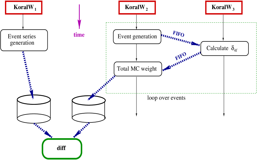
Figure 3: Test KWspecial of the FIFO usage employing two concurrent processes of KoralW. The output is compared (using “diff”) with the output of the standard run of KoralW.

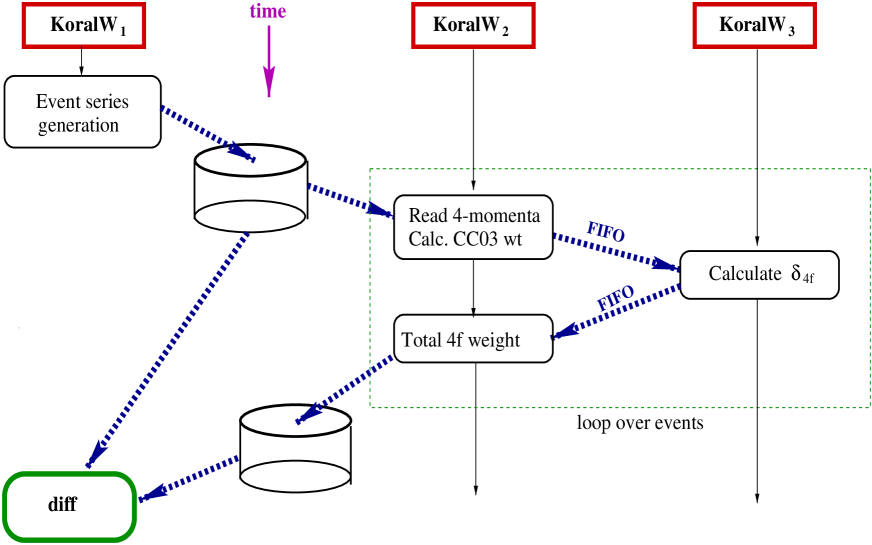
Figure 4: Test KWspecialDisk of the FIFO usage employing two concurrent processes of KoralW. The output is compared (using “diff”) with the output of the standard run of KoralW.

• make KWspecial – a technical test of the FIFO mechanism used in the event reweighting. If you work in the X environment, consider make XKWspecial instead. This important testing demo program is schematically depicted in Fig. 3. The demo goes as follows:

  1. At the beginning, a single run of KoralW₁ in the four-fermion mode is performed in order to generate a benchmark output file.

  2. Next, the true demo begins. The first, master, KoralW₂, located in the directory work.tmp, is started. It generates a series of four-fermion events and writes the four-vectors to the FIFO special file 4vect.data.special. After each set of four-vectors is written, the master KoralW₂ suspends and waits for further input.

  3. Simultaneously, the second, slave, KoralW₃ is executed, also in the four-fermion mode, in the work directory. It reads a single set of four-vectors from the FIFO special file 4vect.data.special, calculates the wtset weights with the CC03 and CCall matrix elements, writes wtset down to another FIFO special file – wtext.data.special and suspends itself.

  4. Finally, the master KoralW₂ resumes execution and reads from the FIFO file wtext.data.special the weight wtset calculated by the slave process. These new wtsets overwrite the original values and the construction of the event is completed by the master process.

  5. After generation, the output file from the master program is compared with the benchmark one generated at the beginning. Apart from the value of a few switches, responsible for read/write operations, there should be no numerical differences between the outputs.

• make KWspecialEXT – similar to the make KWspecial demo with two exceptions: the master KoralW₂ runs in the CC03 mode and instead of the whole wtset vector, only the single correction weight wtEXT is passed back from the slave to the master process. This correction weight is then included in all wtsets of the master process. In particular, it means that all the so-called CC03 weights of the master process get upgraded to the four-fermion level. This is reflected in the comparison of the outputs, where the “upgraded CC03” cross section is compared with the original four-fermion of the benchmark run.

• make KWspecialDISK – similar to the make KWspecialEXT demo with the only difference that the master KoralW₂ reads four-vectors from the disk instead of generating them. The four-vectors were generated by the introductory “benchmark” run of KoralW₁. This demo shows how the CMC solution based on the FIFO mechanism can act as a single MC-like program, reweighting events stored on the disk.

7.4 Demo of the CMC KoralW$\&$YFSWW with the FIFO mechanism

• make KandY – this is the most important demo, showing how to generate four-fermion events with the ${\cal O}(\alpha)$ NL corrections as a result of concurrent runs of KoralW and YFSWW3 with the help of the FIFO (“named pipes”) mechanism. If you work in the X environment, consider make XKandY instead. The demo works as follows:

  1. Two FIFO special files, 4vect.data.special and wtext.data.special, are created and linked to the appropriate input/output file names in the local working directories of KoralW and YFSWW3. The YFSWW3 distribution directory is located next to the KoralW one and the working directory of YFSWW3 is the demo.koralw one. The default input data file common for both programs is the one of KoralW; two additional input data files, with the (optional) information specific to each program, are located in the corresponding working directories.

  2. The master KoralW run is started in the regular mode that generates four-fermion events and writes down the four-vectors of each event to the FIFO special file 4vect.data.special.

  3. Simultaneously the slave run of YFSWW3 is started in the mode that reads the four-vectors from the FIFO special file 4vect.data.special and then writes the ${\cal O}(\alpha)$ NL correction weight back into the other FIFO special file wtext.data.special.

  4. Finally, KoralW reads the ${\cal O}(\alpha)$ NL correction weight from the special file wtext.data.special, combines it with all wtset weights in an additive way and completes the generation of the events with both the four-fermion and ${\cal O}(\alpha)$ corrections included. Optionally, the rejection to the constant-weight events could be performed at this point.

7.5 X-based versions of some demos with FIFO

• make XKWspecial – the version of make KWspecial for the X Window System environment.

• make XKandY – the version of make KandY for the X Window System environment.

7.6 Old tests from demo.14x directory

After installing the package, it is also recommended to execute the commands make KWdemoCC03, make KWdemoGRCall, make KWdemo2HADR and make KWdemo2SEMI from the demo.14x directory, and to compare the outputs against the appropriate Linux benchmark files.

8 Summary and Conclusions

We described the new version 1.51 of the KoralW Monte Carlo event generator for all $e^{+}e^{-}\to f_{1}\bar{f}_{2}f_{3}\bar{f}_{4}$ processes. The basic physics content of the KoralW program has not changed in the version 1.51, except for the reduction/extrapolation procedures. However, a number of technical improvements have been added. They are motivated by the needs of the data analysis at LEP2. As the precision of the measurements related to the $W$-pair production has increased, it has become clear that the complete electroweak perturbative ${\cal O}(\alpha)$ calculation for the $e^{-}e^{+}\to W^{-}W^{+}$ process has to be included. We have found that the most economic way of including the missing EW ${\cal O}(\alpha)$ correction to the KoralW Monte Carlo event generator is to include them in the process of generating each MC event with the help of an additional correcting weight provided by the YFSWW3 program, i.e. to do it in an event-per-event manner.

This requires, of course, sending every MC event generated by KoralW to YFSWW3 in order to get a correction weight. At the technical level this is organized in two ways:

1. The constant-weight events from KoralW are stored on the disk/tape and reprocessed at a later time with the help of YFSWW3 version 1.16 in order to include the missing correction. The appropriate facilities to read the events from disk and calculate weights are now implemented in KoralW and YFSWW3.

2. We also provide a new option in which KoralW and YFSWW3 communicate in real time using the UNIX/Linux standard tool, the FIFO mechanism (named pipes), in order to correct each event generated by KoralW with the weight provided by YFSWW3, accounting for the missing ${\cal O}(\alpha)$ corrections. The important advantage of this solution is that there is no need to modify any part of the two source codes. From the user’s point of view this solution, which we call the “Concurrent Monte Carlo (CMC) KoralW$\&$YFSWW3”, behaves as a regular Monte Carlo event generator of constant-weight events with all of its normal features, a single input/output for example.

It has to be stressed that the distributions and cross sections resulting from our new CMC KoralW$\&$YFSWW3 include both the complete ${\cal O}(\alpha)$ corrections to the $WW$ production process in the LPA and the corrections due to the so-called background diagrams. The CMC KoralW$\&$YFSWW3 fulfills almost completely the requirements of the LEP2 data analysis for the $WW$ process. It is at the moment the only MC program with constant-weight events for this kind of process.

In addition, we have made in KoralW certain modifications that are useful for the studies of the “contamination” of the two-fermion processes by the four-fermion processes. As it was proposed in [30], upon adding the virtual-pair corrections from the $\cal KK$MC program, one can obtain the QED ${\cal O}(\alpha^{2}$) prediction (including the ${\cal O}(\alpha$) EW corrections) for the $e^{-}e^{+}\to f\bar{f}$ process, for the realistic experimental event selection, based entirely on the Monte Carlo simulations, without any use of the semi-analytical calculations. To this end, in the present KoralW version 1.51 we introduce a new extrapolation/reduction procedure, better suited to the relevant processes, which are dominated by the large $t$-channel contributions. They are based on the LL concept of the independent emission of photons and fermion pairs.

Appendix: New and Modified Program Parameters

Variable	Position and meaning
ifphot	xpar(1074) (=1)
	=2 PHOTOS is ON, radiation from quarks and leptons (for tests)
KeyMix	xpar(1041) (=1) – default value changed to 1
KeyBra	xpar(1021) (=1)
	=1 arbitrary values from input, no consistency checks
	=3 values pre-set in the source code
KeyCul	xpar(1014) (=2)
	=2 screened Coulomb correction, new default
KeyISR	xpar(1011) (=1)
	=2 ISR is ON, extrapolation procedure as in YFSWW3
	=3 ISR is ON, extrapolation procedure for $t$-channel-dominated processes

Table 4: The list of input parameters of the KoralW generator modified in version 1.51. Only the modified settings are shown. The default values are in brackets.

Variable	Position and meaning
i_pres	xpar(1079) (=0)
	=1 monitor of presampler probabilities is ON
	=0 monitor of presampler probabilities is OFF
i_yfs	=xpar(1080) (=0) previously dipswitch i_yfs in karludw.f
	=0 photonic internal tests OFF
	=1 photonic internal tests ON
i_file	xpar(1081) (=1) previously dipswitch i_file in karludw.f
	=1 pretabulated spectra for photonic presampling
	=0 spectra for photonic presampling from analytic function
i_disk	=xpar(1082) (=0) previously dipswitch msdump in karludw.f
	=0 normal MC generation of events
	=1 technical; 4f phase space debug mode (reads 4-vectors from disk)
	=2 reading event in PDG-like format:
	four-momenta of final fermions, multiplicity and four-momenta of photons
	=3 reading event in one of two possible formats: character*1 marker
	different from “E” followed by PDG-like event record of i_disk=2,
	or end-of-run marker “E”.
	=4 reading event in one of possible three formats:
	character*1 marker different from “R” and “E” followed by PDG-like
	event record and MC weight, or marker “R” (rejected event)
	followed by PDG-like event record and weight, or end-of-run marker “E”

Table 5: The list of new input parameters of the KoralW generator version 1.51. The default values are in brackets.

Variable	Position and meaning
i_prnt	=xpar(1083) (=1) previously dipswitch kardmp in KW.f
	=0 printout on weight over maximal weight OFF
	=1 printout on weight over maximal weight ON
i_sw4f	=xpar(1084) (=1)
	=–1 all approximations set in data set /isw4f/ in amp4f.f
	=0 CC03
	=1 complete four-fermion
	=2 ISNSγ+Z $\tau^{+}\tau^{-}$ pair emission in $e^{+}e^{-}\to\mu^{+}\mu^{-}$ process.
	=3 FSNSγ+Z $\tau^{+}\tau^{-}$ pair emission in $e^{+}e^{-}\to\mu^{+}\mu^{-}$ process.
	=4 ISNSγ +FSNSγ $\tau^{+}\tau^{-}$ or $e^{+}e^{-}$ pair emission in $e^{+}e^{-}\to\mu^{+}\mu^{-}$ process.
	=5 ISNSγ $\tau^{+}\tau^{-}$ or $e^{+}e^{-}$ pair emission in $e^{+}e^{-}\to\mu^{+}\mu^{-}$ process.
	=6 FSNSγ+Z $\mu^{+}\mu^{-}$ pair emission in $e^{+}e^{-}\to\tau^{+}\tau^{-}$ process.
i_prwt	=xpar(1085) (=4) previously dipswitch i_principal_weight in KW.f
	=2 first-order ISR in principal weight for rejection
	=3 second-order ISR in principal weight for rejection
	=4 third-order ISR in principal weight for rejection
i_writ_wt	=xpar(1086) (=0)
	=0 writing weights on disk OFF
	=1 wtext written on disk
	=2 wtset(1-9) written on disk
i_writ_4v	=xpar(1087) (=0)
	=0 writing four-vectors on disk OFF
	=2 four-vectors written on disk, format as in i_disk=2;
	(readable by i_disk=2)
	=3 four-vectors written on disk, format as in i_disk=3;
	(readable by i_disk=3)
	=4 four-vectors written on disk, format as in i_disk=4;
	(readable by i_disk=4)
i_read_wt	=xpar(1088) (=0)
	=0 reading weights from disk OFF
	=1 reads wtext, combines additively
	=2 reads wtext, combines multiplicatively
	=3 reads wtset(1-9), overwrites original values
	=4 reads wtset(1-9), puts them into wtset(91-99)
	=–3 tests: reads wtset(1-9) and compares with original
	=–2 tests: reads wtext and compares with original 4f weight
	=–1 tests: reads wtext and compares with original CC03 weight

Table 6: (cont.): The list of new input parameters of the KoralW generator version 1.51. The default values are in brackets.

Figure 5: The comparison of the reduction procedures in KoralW and YFSWW3. On the lower plots they are different, i.e. in KoralW we keep that of 1.41, while in the upper plot they are the same, i.e. in KoralW it is adjusted to be the same as in YFSWW3. Plotted are the distributions of the $W^{+}$ polar angle w.r.t. the $e^{+}$ beam and of the angle between the hardest photon with respect to the nearest final-state charged fermion at $\sqrt{s}=500$ GeV.

Figure 6: The technical test of the universality of $d\sigma_{R}$ from YFSWW3 and KoralW. Plotted are the distributions of the $W^{+}$ mass and of the $W^{+}$ polar angle w.r.t. the $e^{+}$ beam at $\sqrt{s}=200$ GeV.

Figure 7: The technical test of the universality of $d\sigma_{R}$ from YFSWW3 and KoralW. Plotted are the distributions of the angle of the photon w.r.t. the $e^{+}$ beam and the sum of the photon energy at $\sqrt{s}=200$ GeV.

Figure 8: The calibration of the CMC KoralW$\&$YFSWW3 (labeled “KandY”) using YFSWW3 for $d\sigma^{\rm{\cal O}(\alpha)+ISR_{23}+Cc}$ at $\sqrt{s}=200$ GeV. Plotted are the distributions of the $W^{+}$ invariant mass and of the $W^{+}$ polar angle w.r.t. the $e^{+}$ beam and their relative differences (diamonds on the lower pictures). We also include the plots for the relative size of the $4f$ background corrections (dots) and of the ${\cal O}(\alpha)$ NL (stars).

Figure 9: The calibration of the CMC KoralW$\&$YFSWW3 (labeled “KandY”) using YFSWW3 for $d\sigma^{\rm{\cal O}(\alpha)+ISR_{23}+Cc}$ at $\sqrt{s}=200$ GeV. Plotted are the distributions of the hardest photon energy and of the photon angle w.r.t. the $e^{+}$ beam, and their relative differences (diamonds on the lower pictures). We also include the plots for the relative size of the $4f$ background corrections (dots) and of the ${\cal O}(\alpha)$ NL (stars).

References

- [1] S. Jadach et al., Comput. Phys. Commun. 119, 272 (1999).
- [2] S. Jadach et al., The Monte Carlo Event Generator YFSWW3 version 1.16 for W-Pair Production and Decay at LEP2/LC Energies, preprint CERN-TH/2001-017, UTHEP-01-0101, January 2001; hep-ph/0103163; submitted to Comput. Phys. Commun.
- [3] Reports of the Working Groups on Precision Calculations for LEP2 Physics, edited by S. Jadach, G. Passarino, and R. Pittau (CERN 2000-009, Geneva, 2000).
- [4] M. Skrzypek, S. Jadach, W. Płaczek, and Z. Wa̧s, Comput. Phys. Commun. 94, 216 (1996).
- [5] M. Skrzypek et al., Phys. Lett. B372, 289 (1996).
- [6] M. Skrzypek and Z. Wa̧s, Comput. Phys. Commun. 125, 8 (2000).
- [7] J. Fujimoto et al., GRACE User’s manual, version 2.0, GRACE User’s manual, version 2.0, MINAMI-TATEYA collaboration.
- [8] F. Caravaglios and M. Moretti, Z. Phys. C74, 291 (1997).
- [9] E. Accomando and A. Ballestrero, Comput. Phys. Commun. 99, 270 (1997).
- [10] G. van Oldenborgh, P. Franzini, and A. Borrelli, Comput. Phys. Commun. 83, 14 (1994).
- [11] D. Charlton, G. Montagna, O. Nicrosini, and F. Piccinini, Comput. Phys. Commun. 99, 355 (1997).
- [12] G. Montagna et al., Higher-order QED corrections to single W production in electron positron collisions, 2000, hep-ph/0005121.
- [13] J. Fujimoto et al., Comput. Phys. Commun. 100, 128 (1997).
- [14] A. Pukhov et al., CompHEP: A package for evaluation of Feynman diagrams and integration over multi-particle phase space. User’s manual for version 33, 1999, hep-ph/9908288.
- [15] A. Kanaki and C. G. Papadopoulos, HELAC-PHEGAS: Automatic computation of helicity amplitudes and cross sections, 2000, hep-ph/0012004.
- [16] R. Miquel and M. Schmitt, Z. Phys. C71, 251 (1996).
- [17] H. Anlauf, P. Manakos, T. Ohl, and H. Dahmen, WOPPER, Version 1.5: A Monte Carlo Event Generator for at LEP-2 and Beyond., 1996, IKDA-96-15, hep-ph/9605457.
- [18] F. A. Berends, C. G. Papadopoulos, and R. Pittau, NEXTCALIBUR: A four-fermion generator for electron positron collisions, 2000, hep-ph/0011031.
- [19] C. Papadopoulos, Comput. Phys. Commun. 101, 183 (1997).
- [20] S. Jadach, W. Płaczek, M. Skrzypek, and B. F. L. Ward, Phys. Rev. D54, 5434 (1996).
- [21] S. Jadach et al., Phys. Lett. B417, 326 (1998).
- [22] S. Jadach et al., Phys. Rev. D61, 113010 (2000).
- [23] S. Jadach et al., Precision predictions for (un)stable W+W- production at and beyond LEP2 energies, preprint CERN-TH/2000-337; hep-ph/0007012; submitted to Phys. Lett. B.
- [24] A. Denner, S. Dittmaier, M. Roth, and D. Wackeroth, Nucl. Phys. Proc. Suppl. 89, 100 (2000).
- [25] A. Denner, S. Dittmaier, M. Roth, and D. Wackeroth, Nucl. Phys. B587, 67 (2000).
- [26] J. Fleischer, F. Jegerlehner, and M. Zrałek, Z. Phys. C42, 409 (1989).
- [27] K. Kołodziej and M. Zrałek, Phys. Rev. D43, 3619 (1991).
- [28] J. Fleischer, K. Kołodziej, and F. Jegerlehner, Phys. Rev. D47, 830 (1993).
- [29] J. Fleischer, F. Jegerlehner, K. Kołodziej, and G. J. van Oldenborgh, Comput. Phys. Commun. 85, 29 (1995).
- [30] M. Kobel et al., Two-fermion production in electron-positron collisions, in Ref. [3], p. 269.
- [31] D. E. Groom et al., Eur. Phys. J. C15, 1 (2000).
- [32] E. Barberio, B. van Eijk, and Z. Wa̧s, Comput. Phys. Commun. 66, 115 (1991), ibid. 79 291 (1994).
- [33] A. P. Chapovsky and V. A. Khoze, Eur. Phys. J. C9, 449 (1999).
- [34] T. Ishikawa, Y. Kurichara, M. Skrzypek, and Z. Wa̧s, Eur. Phys. J. C4, 75 (1998).
- [35] J. Alberty et al., in Perspectives for new detectors in future supercolliders, Proceedings of the Workshop of the INFN Eloisatron Project, October 1989, Erice, Italy, edited by L. Cifarelli, R. Wigmans, and T. Ypsilantis (World Scientific, Singapore, 1989), p. 170.
- [36] M. Grünewald et al., Four-fermion production in electron-positron collisions, in Ref. [3], p. 1.
- [37] S. Jadach, B. F. L. Ward, and Z. Wa̧s, Comput. Phys. Commun. 130, 260 (2000).
- [38] D. Bardin et al., in Proceedings of the Zeuthen Workshop on Elementary Particle Theory - Physics at LEP200 and Beyond, Teuplitz, Germany, edited by T. Riemann and J. Blümlein (Nucl. Phys. (Proc. Suppl.), B37, 1994).
- [39] M. Jeżabek, Z. Wa̧s, S. Jadach, and J. H. Kühn, Comput. Phys. Commun. 70, 69 (1992).
- [40] R. Decker, S. Jadach, J. H. Kühn, and Z. Wa̧s, Comput. Phys. Commun. 76, 361 (1993).
- [41] P. Golonka, E. Richter-Wa̧s, and Z. Wa̧s, The TAUOLA-PHOTOS-F environment for versioning the TAUOLA and PHOTOS packages, hep-ph/0009302.
- [42] T. Pierzchała, E. Richter-Wa̧s, Z. Wa̧s, and M. Worek, Acta Phys. Polon. B32, 1277 (2001).