Cancellation of Sudakov Logarithms in Radiative Decays of Quarkonia

F. Hautmann

Department of Physics, Pennsylvania State University, University Park PA 16802

Abstract

We study infrared QCD effects in radiative quarkonia decays. We examine the endpoint region $z\to 1$ of the photon spectrum. We point out a cancellation mechanism for the corrections in $\alpha_{s}^{n}\ln^{m}(1-z)$, $m\leq 2n$, in the short-distance coefficient for the color-singlet Fock state in the quarkonium. The cancellation is due to the coherence of the color radiation, and applies even though logarithmic contributions are present in the jet distributions associated with the decay. We comment on the implications of our results for the modeling of hadronization in the endpoint region and for the role of color-octet states in the quarkonium.

PSU-TH/236

February 2001

1. Introduction

Radiative decays of heavy quark-antiquark bound states (quarkonia) have been investigated in the framework of perturbative QCD and have been used to measure the QCD coupling at energies of the order of the heavy quark mass $m$ [1, 2, 3, 4]. The use of perturbative QCD in this context is based on the fact that, as long as the velocity $v$ of the heavy quark is small, these decay processes involve two widely separated distance scales: the scale $1/(mv^{2})$ over which the quark and antiquark bind into the quarkonium and the scale $1/m$ over which the quark-antiquark pair decays. By expanding about the nonrelativistic limit $v\to 0$, one may treat the process as the product of a long-distance, nonperturbative factor, containing all of the bound-state dynamics, and a short-distance factor, describing the annihilation of the heavy quark pair and computable as a power series expansion in $\alpha_{s}$.

However, near the exclusive boundary of the phase space, where the photon’s energy approaches its kinematic limit, both the expansion to fixed order in $v$ and the expansion to fixed order in $\alpha_{s}$ become inadequate to represent correctly the physics of the decay. On one hand, classes of relativistic corrections that by power counting are higher order in $v$ become enhanced by powers of $1/\alpha_{s}$ [5, 6, 7]. On the other hand, potentially large terms in $\ln(1-z)$ (with $1-z$ being the parameter that measures the distance from the endpoint) appear in the coefficients of the expansion in $\alpha_{s}$ to all orders [8]. In both cases, reliable results can only be obtained after resummation of the enhanced contributions.

Infrared QCD effects are responsible for these behaviors. Soft color interactions account for the heavy quark-antiquark pair turning into a color-octet state, whose contribution, although subleading in $v$, becomes important near the endpoint. Sudakov logarithms in $1-z$ arise as remnants of the imperfect cancellation of the infrared divergences in the exclusive region, where particle production is suppressed. The need for resummations noted above is a symptom of the sensitivity of the process to contributions from infrared scales. A corresponding effect is seen in calculations that incorporate models for the hadronization of partons [4, 9, 10], where nonperturbative contributions are found to be essential to describe the endpoint region of the photon energy spectrum in $J/\psi$ [11] and $\Upsilon$ [3, 12] decays.

In this paper we present a treatment of the infrared QCD radiation near the kinematic boundary. We describe contributions from soft and collinear gluons with logarithmic accuracy, and study the color correlations between the jets that accompany the photon. This treatment takes account of the coherence properties of gluon emission. We determine the regions in the final-state phase space for the quarkonium decay in which destructive interference between parton emitters suppresses color radiation.

We use these results to examine potentially large Sudakov logarithms in the photon spectrum. We find (see Sec. 4) that Sudakov logarithms cancel order by order in $\alpha_{s}$ in the short distance coefficient for the color-singlet Fock state in the quarkonium. The cancellation mechanism applies to the leading logarithms as well as to any subleading logarithms. As a result, no Sudakov suppression factor arises near the endpoint.

The picture underlying this behavior can be understood in simple terms based on the branching formulas for the decay discussed in Sec. 2. In the boundary kinematics the photon recoils against two almost-collinear gluon jets. The cancellation of Sudakov corrections reflects the fact that color is neutralized already at the level of this two-jet configuration. This situation may be contrasted with the situation one encounters in the decay of an electroweak gauge boson into jets. Here Sudakov corrections arise precisely from the presence of color charges in two-jet configurations.

This picture also indicates that no cancellation should occur for the color-octet Fock state in the quarkonium. In this case, we expect the usual Sudakov suppression to take place near the endpoint of the photon spectrum. Then one of the consequences of the results of this paper concerns the ratio of the color-octet to the color-singlet contributions. This ratio will be smaller than expected from the power counting in $v$ and $\alpha_{s}$ obtained by truncating perturbation theory to fixed order [5, 13, 14], owing to the different high order behavior of the perturbation series in the two cases.

A preliminary discussion of the results presented in this paper appeared in Ref. [15].

The paper is organized as follows. In Sec. 2 we treat the emission of soft and collinear gluons associated with the quarkonium decay. This leads us to a general branching formula. In Sec. 3 we evaluate the phase space in this formula. In Sec. 4 we compute the photon spectrum and observe the cancellation of the Sudakov logarithms. In Sec. 5 we discuss the implications of our results and give conclusions.

2. Infrared radiation near the phase space boundary

In this section we describe the QCD radiation that accompanies the decay of the quarkonium near the endpoint of the photon spectrum. The key element in our treatment is the coherent emission of gluons and the angular ordering of this emission. We arrive at an expression for the photon spectrum that is valid to leading and next-to-leading accuracy in the soft and/or collinear logarithms.

We consider the decay of a quarkonium state $H$ of mass $M$ into a photon plus anything:

$$H\to\gamma+X\hskip 14.22636pt.$$ (1)

We concentrate on the case of the leading Fock state for a ${}^{3}S_{1}$ quarkonium state, that is, a heavy quark-antiquark pair in a color singlet state.

This decay receives contributions at the leading order of perturbation theory both when the photon is directly coupled to the heavy quarks (direct term) and when the photon is produced by collinear emission from light quarks (fragmentation term) [16]. In the endpoint region the fragmentation contribution is suppressed relative to the direct term. The discussion of this paper will thus focus on the direct term.

2.1 Notations and tree-level decay

The direct contribution at the leading order is given by the process

$$H(P)\to\gamma(k)+g(k_{1})+g(k_{2})\hskip 14.22636pt$$ (2)

evaluated at the tree level. We introduce dimensionless energy variables for the particles in the final state, as follows

$$z={{2P\cdot k}\over{M^{2}}}\hskip 2.84544pt,\hskip 8.5359ptx_{i}={{2P\cdot k_{i}}\over{M^{2}}}\hskip 2.84544pt,\hskip 8.5359pti=1,2\hskip 17.07182pt.$$ (3)

In the quarkonium rest frame $z$ and $x_{i}$ are respectively the photon and gluon energies scaled by the heavy quark mass $m$ ($m\simeq M/2$ in the lowest nonrelativistic approximation).

The normalized photon spectrum from the process (2) is given by [17]

$${1\over\Gamma_{0}}\ {{d\Gamma_{0}}\over{dz}}={1\over{\pi^{2}-9}}\ \int_{0}^{1}dx_{1}\int_{0}^{1}dx_{2}\ \rho(x_{1},x_{2},z)\ \delta(z-2+x_{1}+x_{2})\ \Theta(x_{1}+x_{2}-1)\hskip 2.84544pt,$$ (4)

with

$$\rho(x_{1},x_{2},z)={{(1-x_{1})^{2}}\over{z^{2}x_{2}^{2}}}+{{(1-x_{2})^{2}}\over{z^{2}x_{1}^{2}}}+{{(1-z)^{2}}\over{x_{1}^{2}x_{2}^{2}}}\hskip 11.38092pt.$$ (5)

Over almost the entire range in $z$ the result (4) is well approximated by a spectrum rising linearly with $z$. At the endpoint, however, the first derivative of the spectrum (4) is singular. We will come back to this in Sec. 4.

2.2 Behavior at $z\to 1$

Beyond the tree level, corrections in $\ln(1-z)$ to the spectrum become possible [8]. These come from the infrared region: near the endpoint the emission of gluons is suppressed and terms in $\ln(1-z)$ result from the imperfect cancellation of the infrared divergences between real and virtual graphs. The contribution from the soft and/or collinear gluons associated with the decay is at most double-logarithmic for each power of $\alpha_{s}$. By power counting the leading behavior of the photon spectrum as $z\to 1$ is of the type [8]

$${1\over\Gamma}\ {{d\Gamma}\over{dz}}\sim{\mbox{const.}}\ +\sum_{k=1}^{\infty}c_{k}\ \alpha_{s}^{k}\ \ln^{2k}(1-z)\;\;,\;\;\;\;\;z\to 1\hskip 11.38092pt.$$ (6)

In this paper we will see a cancellation mechanism for these corrections that works order by order in perturbation theory. A qualitative picture of the cancellation that we will discuss in the next sections can be given at one loop as follows. Consider the emission of a soft gluon with momentum $q$ from the tree-level graphs for the decay (2). In the leading infrared approximation, the amplitude ${\cal A}$ for this process factorizes (see for instance [18]) into a nonabelian, classical current ${\bf j}(q)$, describing the soft-gluon emission, times the tree level amplitude ${\cal A}_{0}$:

$${\cal A}^{b}(P,k_{1},k_{2};q)\simeq g_{s}\varepsilon^{\mu}(q){\bf j}_{\mu}^{b}(q){\cal A}_{0}(P,k_{1},k_{2})\hskip 11.38092pt,$$ (7)

where $\varepsilon$ is the gluon polarization vector, $b$ is the gluon color index, and

$${\bf j}^{\mu}(q)=\sum_{i}{\bf T_{i}}{k^{\mu}_{i}\over{k_{i}\cdot q}}\hskip 11.38092pt.$$ (8)

Here the sum runs over the final-state colored particles $k_{1}$ and $k_{2}$, and ${\bf T_{i}}$ are the color matrices associated with the coupling of the soft gluon to each of these particles. There is no contribution from the coupling to quarks: the coupling to the virtual quark lines is subleading in the infrared limit because these lines are off shell by order $M$; the coupling to the quark and antiquark in the quarkonium does not contribute either, although these quarks are nearly on shell, because in the lowest nonrelativistic approximation they are almost collinear and their total color charge is zero.

To the approximation at which we are working, the phase space also factorizes [18], so that one gets a factorized answer for the spectrum, schematically of the form

$${{d\Gamma}\over{dz}}\simeq\alpha_{s}\int{\bf j}^{2}\,{{d\Gamma_{0}}\over{dz}}\,d\Phi^{\prime}\hskip 11.38092pt.$$ (9)

Here $d\Phi^{\prime}$ is the Lorentz-invariant phase space for the soft gluon emission. The standard power counting in terms of the soft gluon energy $\omega$ gives

$$d\Phi^{\prime}\sim\omega\,d\omega\,d\Omega\hskip 5.69046pt,\hskip 11.38092pt{\bf j}^{2}\sim{1\over{\omega^{2}}}\,{{k_{1}\cdot k_{2}}\over{f(z;{\mbox{angles}})}}\hskip 11.38092pt,$$ (10)

where $d\Omega$ is the angular phase space, and $f$ is a function of $z$ and the angles as $\omega\to 0$. Up to the first order in $\omega$ the correlation of the gluon momenta is

$$k_{1}\cdot k_{2}\sim M^{2}\left[(1-z)+{\omega\over M}\,g(z;{\mbox{angles}})\right]\hskip 11.38092pt.$$ (11)

That is, as $z\to 1$ the photon recoils against two almost-collinear hard gluons. In this configuration, the logarithmic integration $d\omega/\omega$ in Eq. (9) is canceled. The next few sections are devoted to showing that this is indeed the mechanism that dominates the radiation accompanying the decay, and that it extends to all orders in $\alpha_{s}$.

The back-to-back kinematics suggests an analogy with the two-jet region in the annihilation of $e^{+}e^{-}$ into electroweak gauge bosons. Since the two jets are now in a singlet, though, the pattern of color correlations will be different. Jet event shapes in $e^{+}e^{-}$ annihilation have been studied extensively by using methods based on branching graphs. We will see in the remainder of this section that the photon spectrum in decays of quarkonia can be treated in a similar manner. The subtlest point will be the treatment of the branching phase space. This will be addressed in Sec. 3.

2.3 Branching graphs

Methods to calculate multi-parton matrix elements in the leading soft and collinear orders have been known for a long time. See Ref. [18] for a review. The essential observation in these methods is that one can replace the calculation of higher-loop Feynman graphs by the calculation of angular-ordered “branching” graphs, that is, tree level graphs in which the angular phase space is subject to certain ordering constraints at each branching. The method has also been extended to include next-to-leading logarithms: see for instance Ref. [19]. In this and the next subsection we apply this approach to the quarkonium decay.

We write the energy spectrum $d\Gamma/dz$ in the inclusive decay (1) in terms of the exclusive decay widths $d\Gamma_{n}^{(\rm{excl})}$ for producing $\gamma$ $+$ $n$ final state partons $q_{1},\dots,q_{n}$:

$${1\over\Gamma}\ {{d\Gamma}\over{dz}}=\sum_{n=2}^{\infty}{1\over\Gamma}\int d\Gamma_{n}^{(\rm{excl})}(q_{1},\dots,q_{n})\delta\left(z-2+\sum_{i}{{2P\cdot q_{i}}\over{M^{2}}}\right)\hskip 5.69046pt.$$ (12)

Here the $\delta$ function expresses the photon energy fraction $z$ in terms of the quarkonium and parton momenta. The exclusive decay widths are generated by the branching process [18, 19, 20].

The first step of the branching corresponds to the lowest order final state, Eq. (2), in which the photon is accompanied by two gluons with invariant mass $(k_{1}+k_{2})^{2}$. This invariant mass provides the basic mass scale at the hard end of the branching. The subsequent steps correspond to consecutive parton splittings (Fig. 1a). There are well-defined probability weights associated with each splitting vertex, and form factors associated with each line connecting two vertices [18, 19]. The basic point about the branching process is that the phase space for the splittings is restricted to the angular ordered region in which the branching angles decrease as we go from the parent parton toward the final state. If we denote, as in Fig. 1a, by $y_{i}$ the energy transfer at the vertex $i$, and by $r_{\perp i}$ the transverse momentum flowing between vertices $i$ and $i+1$, this region is defined (for small $y_{i}$) by

$$(k_{1}+k_{2})^{2}\ \hbox{\raise 2.0pt\hbox{$>$} \kern-13.0pt\lower 3.0pt\hbox{$\sim$}}\ {{r_{\perp 1}^{2}}\over y_{1}^{2}}\ \hbox{\raise 2.0pt\hbox{$>$} \kern-13.0pt\lower 3.0pt\hbox{$\sim$}}\ {{r_{\perp 2}^{2}}\over{y_{1}^{2}\ y_{2}^{2}}}\ \hbox{\raise 2.0pt\hbox{$>$} \kern-13.0pt\lower 3.0pt\hbox{$\sim$}}\ \dots\hskip 5.69046pt.$$ (13)

The reason for the angular ordering is a coherence effect: outside the ordered region parton emitters interfere destructively [20, 21, 22]. In this approach, the exclusive decay width $d\Gamma_{n}^{(\rm{excl})}$ is obtained by taking all angular-ordered branching graphs with $n$ final state partons, and summing the corresponding probability weights.

Following [19], we integrate the exclusive decay widths over the phase space of the final state partons keeping $k_{1}$ and $k_{2}$ fixed. We rewrite the $n$-parton phase space as (Fig. 1b)

$$\left[\prod_{j=1}^{n}{{d^{4}q_{j}}\over{(2\pi)^{3}}}\delta_{+}(q_{j}^{2})\right] = d^{4}k_{1}\delta^{4}\left(k_{1}-\sum_{j=1}^{l}q_{j}\right)\left[\prod_{j=1}^{l}{{d^{4}q_{j}}\over{(2\pi)^{3}}}\delta_{+}(q_{j}^{2})\right]$$ (14)

$$\times d^{4}k_{2}\delta^{4}\left(k_{2}-\sum_{j=l+1}^{n}q_{j}\right)\left[\prod_{j=l+1}^{n}{{d^{4}q_{j}}\over{(2\pi)^{3}}}\delta_{+}(q_{j}^{2})\right]\hskip 11.38092pt.$$

The integration of the branching matrix element over the final state phase space at fixed $k_{i}^{2}$ ($i=1,2$) produces the jet mass distribution $J_{g}(p^{2},k_{i}^{2})$ [19]. This is defined as the probability to generate a jet with invariant mass $k_{i}^{2}$ from a parent gluon produced at the mass scale $p^{2}$. We have

$$J_{g}\left((k_{1}+k_{2})^{2},k_{1}^{2}\right) = \left[\prod_{j=1}^{l}{{d^{4}q_{j}}\over{(2\pi)^{3}}}\delta_{+}(q_{j}^{2})\right](2\pi)^{4}\delta^{4}\left(k_{1}-\sum_{j=1}^{l}q_{j}\right)$$ (15)

$$\times ({\mbox{branching}}\hskip 5.69046pt{\mbox{matrix}}\hskip 5.69046pt{\mbox{element}})\hskip 11.38092pt,$$

and an analogous expression for $J_{g}\left((k_{1}+k_{2})^{2},k_{2}^{2}\right)$. Note that the jet mass distributions depend on the mass scale $(k_{1}+k_{2})^{2}$. As implied by the coherence relation (13), this is the mass scale at which the initial gluons in the branching are produced.

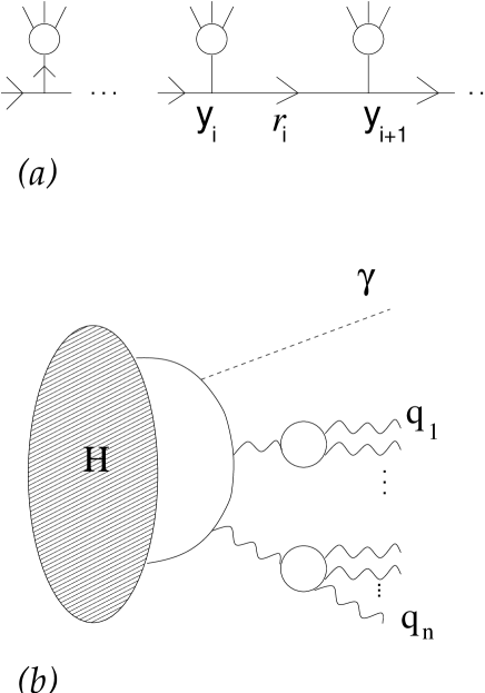
Figure 1: (a) Branching process; (b) final states in the quarkonium decay.

2.4 Jet mass distributions and inclusive spectrum

To lowest order, there is only one final state parton in the definition (15) of the jet mass distribution, and $J_{g}$ is just given by a delta function:

$$J_{g}\left(p^{2},k^{2}\right)=\delta(k^{2})+{\cal O}(\alpha_{s})\hskip 5.69046pt.$$ (16)

In general, the analysis of the jet branching process allows one to obtain an evolution equation [19] for the jet mass distribution. Schematically, this has the form

$$J(p^{2},k^{2})=\delta(k^{2})+\int\alpha_{s}(p^{\prime 2}){\cal K}(p^{\prime 2},k^{2})\otimes J(p^{\prime 2},k^{2})\;\;\;,$$ (17)

where ${\cal K}$ is a kernel calculable as a power series expansion in $\alpha_{s}$. Expressions for the kernel ${\cal K}$ are known to the leading [18, 20, 22] and next-to-leading order [19, 23]. Solving the evolution equation to the leading logarithms gives

$$\int dk^{2}\ J_{g}(p^{2},k^{2})\ \Theta(K^{2}-k^{2})=\exp\left[\ln\left({p^{2}\over K^{2}}\right)f\left(\beta_{0}\alpha_{s}\ln\left({p^{2}\over K^{2}}\right)\right)\right]\hskip 5.69046pt,$$ (18)

where $\beta_{0}=(11C_{A}-2N_{f})/(12\pi)$ and $f$ is the function

$$f(x)=-{C_{A}\over{2\pi\beta_{0}}}\ {1\over x}\ \left[(1-2x)\ \ln(1-2x)-2\ (1-x)\ \ln(1-x)\right]\hskip 5.69046pt.$$ (19)

It is also useful to introduce the double logarithmic approximation. This is defined by expanding the exponent in the right hand side of Eq. (18) to the first order in $\alpha_{s}$. In this approximation, using $f(x)=-C_{A}x/(2\pi\beta_{0})+{\cal O}(x^{2})$, we get

$$\int dk^{2}\ J_{g}(p^{2},k^{2})\ \Theta(K^{2}-k^{2})\approx\exp\left[-{{\alpha_{s}}\over{2\pi}}\ C_{A}\ \ln^{2}\left({p^{2}\over K^{2}}\right)\right]\hskip 5.69046pt.$$ (20)

In order to express the inclusive spectrum in terms of the jet mass distributions, we now use the definitions (14),(15) in Eq. (12). By taking account of the photon phase space factor, the inclusive spectrum takes the form

$${1\over\Gamma}\ {{d\Gamma}\over{dz}} = \int{{d^{4}k}\over{(2\pi)^{3}}}{{d^{4}k_{1}}\over{(2\pi)^{3}}}{{d^{4}k_{2}}\over{(2\pi)^{3}}}(2\pi)^{4}\delta^{4}(P-k-k_{1}-k_{2})\delta\left(z-{{2P\cdot k}\over M^{2}}\right)\delta_{+}(k^{2})$$ (21)

$$\times {\cal M}_{0}(P,k_{1},k_{2})\ J_{g}\left((k_{1}+k_{2})^{2},k_{1}^{2}\right)\ J_{g}\left((k_{1}+k_{2})^{2},k_{2}^{2}\right)\hskip 17.07182pt.$$

Here ${\cal M}_{0}$ is the amplitude for the first step in the branching, with final state $\gamma gg$. Owing to the constraint set by coherence, we can use the approximation $(k_{1}+k_{2})^{2}\gg k_{1}^{2},k_{2}^{2}$ and evaluate ${\cal M}_{0}$ by setting $k_{1}^{2}=k_{2}^{2}=0$. The explicit expression is readily computed and reads

$${\cal M}_{0}={{8\pi^{3}M^{2}}\over{\pi^{2}-9}}\ \left[{{4(k_{1}\cdot k_{2})^{2}}\over{(P\cdot k_{1})^{2}\ (P\cdot k_{2})^{2}}}+{1\over{(P\cdot k)^{2}}}\ \left({{(P-k_{1})^{4}}\over{(P\cdot k_{2})^{2}}}+{{(P-k_{2})^{4}}\over{(P\cdot k_{1})^{2}}}\right)\right]\hskip 17.07182pt.$$ (22)

We are now going to evaluate the branching formula (21) explicitly. To this end, we need to analyze the phase space of this formula in detail. This is the object of the next section.

3. Structure of the phase space for small jet masses

We are interested in the angular-ordered, coherent region

$$k_{1}^{2}\hskip 2.84544pt,\hskip 2.84544ptk_{2}^{2}\ll(k_{1}+k_{2})^{2}\ll M^{2}\hskip 17.07182pt.$$ (23)

Consider the phase space element in Eq. (21):

$$d\Phi=d^{4}k\ d^{4}k_{1}\ d^{4}k_{2}\ \delta^{4}(P-k-k_{1}-k_{2})\ \delta\left(z-{{2P\cdot k}\over M^{2}}\right)\ \delta_{+}(k^{2})\hskip 17.07182pt.$$ (24)

It is convenient to express this phase space in terms of the energy fractions $x_{1}$, $x_{2}$ defined in Eq. (3), the jet masses $k_{1}^{2}$, $k_{2}^{2}$, and

$$s_{12}=(k_{1}+k_{2})^{2}\hskip 17.07182pt.$$ (25)

We can use the momentum conserving $\delta$ in Eq. (24) to integrate over $k$. From the positivity of the jet energies and invariant masses we have

$$0\leq x_{1}\leq 1\hskip 5.69046pt,\hskip 11.38092pt0\leq x_{2}\leq 1\hskip 5.69046pt,\hskip 11.38092ptx_{1}+x_{2}\geq 1\hskip 17.07182pt,$$ (26)

$$0\leq k_{1}^{2}\leq x_{1}^{2}M^{2}/4\hskip 5.69046pt,\hskip 11.38092pt0\leq k_{2}^{2}\leq x_{2}^{2}M^{2}/4\hskip 17.07182pt.$$ (27)

The relation (25) between $s_{12}$ and the jet momenta implies

$$k_{1}^{2}+k_{2}^{2}+{1\over 2}x_{1}x_{2}M^{2}-2|{\bf k}_{1}||{\bf k}_{2}|\leq s_{12}\leq k_{1}^{2}+k_{2}^{2}+{1\over 2}x_{1}x_{2}M^{2}+2|{\bf k}_{1}||{\bf k}_{2}|\hskip 17.07182pt$$ (28)

with $|{\bf k}_{1}|=\sqrt{x_{1}^{2}M^{2}/4-k_{1}^{2}}$, $|{\bf k}_{2}|=\sqrt{x_{2}^{2}M^{2}/4-k_{2}^{2}}$.

The phase space element can then be rewritten as

$$d\Phi={{\pi^{2}M^{2}}\over 4}\ dx_{1}\ dx_{2}\ dk_{1}^{2}\ dk_{2}^{2}\ ds_{12}\ \delta(z-2+x_{1}+x_{2})\ \delta(M^{2}(1-z)-s_{12})\hskip 17.07182pt,$$ (29)

with the constraints (26),(27),(28).

Eq. (28) selects in general a subspace of a complicated form. But we need to consider it in the logarithmic region (23). We may use the $\delta$ functions in Eq. (29) to integrate over $s_{12}$ and one of the energy fractions, say, $x_{2}$. Then Eq. (28) gives

$$x_{1}^{-}\leq x_{1}\leq x_{1}^{+}\hskip 17.07182pt,$$ (30)

with

$$x_{1}^{\pm} = (1-z/2)\ (1-z+k_{1}^{2}/M^{2}-k_{2}^{2}/M^{2})/(1-z)$$ (31)

$$\pm (z/2)\ \sqrt{\left(k_{1}^{2}-k_{2}^{2}\right)^{2}/M^{4}+(1-z)^{2}-2\ (1-z)\left(k_{1}^{2}+k_{2}^{2}\right)/M^{2}}/(1-z)\hskip 17.07182pt.$$

By approximating the constraints (30) for $k_{1}^{2}$, $k_{2}^{2}\ll M^{2}(1-z)\ll M^{2}$, we get

$$x_{1}\ \hbox{\raise 2.0pt\hbox{$>$} \kern-13.0pt\lower 3.0pt\hbox{$\sim$}}\ {{k_{1}^{2}}\over{M^{2}(1-z)}}\hskip 17.07182pt,$$ (32)

and

$$x_{1}\ \hbox{\raise 2.0pt\hbox{$<$} \kern-13.0pt\lower 3.0pt\hbox{$\sim$}}\ 1-{{k_{2}^{2}}\over{M^{2}(1-z)}}\hskip 17.07182pt,$$ (33)

that is, since $1-x_{1}\simeq x_{2}$ for $z\to 1$,

$$x_{2}\ \hbox{\raise 2.0pt\hbox{$>$} \kern-13.0pt\lower 3.0pt\hbox{$\sim$}}\ {{k_{2}^{2}}\over{M^{2}(1-z)}}\hskip 17.07182pt.$$ (34)

Eqs. (32) and (34) tell us that in the coherent region the phase space available for the evolution of each of the jets is bounded by the recoiling jet. For $z\to 1$ this bound is tighter than the bound from the fragmentation of the jet itself, Eq. (27). In the next section we will see that the recoil constraint conspires with the angular-ordered form of the jet mass distribution to destroy any logarithmic hierarchy in the inclusive photon spectrum.

4. The photon spectrum near the endpoint

We now put together the results of Sec. 3 for the phase space with the structure of the spectrum described in Sec. 2 based on the coherent branching.

By using Eqs. (22),(29), (32) and (34) in Eq. (21), we can rewrite the photon energy spectrum as follows:

$${1\over\Gamma}\ {{d\Gamma}\over{dz}} \simeq {1\over{\pi^{2}-9}}\ \int_{0}^{1}dx_{1}\int_{0}^{1}dx_{2}\ \rho(x_{1},x_{2},z)\ \delta(z-2+x_{1}+x_{2})\ \Theta(x_{1}+x_{2}-1)$$ (35)

$$\times \int_{0}^{\infty}dk_{1}^{2}\ J_{g}\left(M^{2}(1-z),k_{1}^{2}\right)\ \Theta(M^{2}x_{1}(1-z)-k_{1}^{2})\ \Theta(M^{2}x_{1}^{2}/4-k_{1}^{2})$$

$$\times \int_{0}^{\infty}dk_{2}^{2}\ J_{g}\left(M^{2}(1-z),k_{2}^{2}\right)\ \Theta(M^{2}x_{2}(1-z)-k_{2}^{2})\ \Theta(M^{2}x_{2}^{2}/4-k_{2}^{2})\hskip 5.69046pt,$$

with $\rho(x_{1},x_{2},z)$ given in Eq. (5). The main structural difference with respect to the case of jet event shapes in $e^{+}e^{-}$ annihilation is that in Eq. (35) there is a two-dimensional integration over a distribution $\rho$ in the energy fractions $x_{1}$, $x_{2}$. This comes from the fact that in quarkonia decays the parton branching is probed by a non-pointlike source. Eq. (35) allows us to discuss the logarithmic behaviors in the endpoint region.

Observe first that, by substituting into Eq. (35) the zeroth-order expression (16) for the jet mass distribution $J_{g}$, we recover the lowest order result (4). So at the lowest order of perturbation theory Eq. (35) gives the correct answer for any $z$. At higher orders of perturbation theory, Eq. (35) gives an approximation valid in the region of large $z$ with leading-logarithm and next-to-leading-logarithm accuracy, provided the jet mass distributions $J_{g}$ are evaluated with corresponding accuracy. Once expanded to the next to lowest order in $\alpha_{s}$, Eq. (35) can be matched with the NLO perturbation theory result [24], and could thus be used to obtain improved predictions, valid over a wider range of $z$.

Eq. (35) enables us to see that, although Sudakov logarithms are present in the jet distributions associated with the decay, the corrections in $\ln(1-z)$ to the photon energy spectrum cancel order by order in $\alpha_{s}$. The mechanism for the cancellation can be seen in its simplest form by using the double-logarithmic approximation (20) for $J_{g}$. By expanding the right hand side of Eq. (20) in powers of $\alpha_{s}$ and substituting this into Eq. (35), we note that the higher order corrections to $d\Gamma/dz$ involve integrals of the form

$$\int_{1-z}^{1}dx_{1}\ln^{k}\left({{M^{2}(1-z)}\over{M^{2}x_{1}(1-z)}}\right)=\int_{1-z}^{1}dx_{1}\ln^{k}(1/x_{1})\hskip 17.07182pt.$$ (36)

That is, logarithmic contributions in $x_{1}$ arise, which are important at the kinematic limit $x_{1}\to 0$, but these never give rise to logarithms of $(1-z)$ in the photon spectrum. Terms in $\ln(1-z)$ cancel because of coherence, i.e., as a result of the constraint (32) on the jet mass and of the angular ordering (13) in the branching.

From Eq. (35) we can obtain an explicit expression for $d\Gamma/dz$ by keeping track of all the leading logarithms in the jet distributions. This is accomplished through Eq. (18). Using this formula in Eq. (35) we get

$${1\over\Gamma}\ {{d\Gamma}\over{dz}} \simeq {1\over{\pi^{2}-9}}\ \int_{0}^{1}dx_{1}\int_{0}^{1}dx_{2}\ \rho(x_{1},x_{2},z)\ \delta(z-2+x_{1}+x_{2})\ \Theta(x_{1}+x_{2}-1)$$ (37)

$$\times \exp\left[\ln(1/x_{1})\ f\left(\beta_{0}\alpha_{s}\ln(1/x_{1})\right)+\ln(1/x_{2})\ f\left(\beta_{0}\alpha_{s}\ln(1/x_{2})\right)\right]\hskip 17.07182pt,$$

where $f(x)$ is given in Eq. (19). It is straightforward to check from Eq. (37), by expanding the integrand in powers of $\alpha_{s}$, that no logarithms of $(1-z)$ appear in the perturbative expansion of $d\Gamma/dz$.

The above results indicate that the photon spectrum from the decay of the color-singlet Fock state in the quarkonium is not Sudakov suppressed by higher orders of perturbation theory in the endpoint region. Higher perturbative corrections give rise to a constant shift compared to the leading order answer (4).

The first derivative of the spectrum, on the other hand, does get logarithmic corrections in $(1-z)$. This can be realized just from Eq. (36) by taking the derivative with respect to $z$. A singularity in the derivative of the spectrum at $z=1$ was indeed noted already in lowest order (see comment below Eq.(5)). The leading logarithmic behavior at one loop will be of the type

$${d\over{dz}}\left({1\over\Gamma}\ {{d\Gamma}\over{dz}}\right) = \left[a_{0}\ln\left(1-z\right)+{\mbox{const}}.+{\cal O}(1-z)^{1}\right]$$

$$+ \alpha_{s}\left[a_{1}\ln^{3}\left(1-z\right)+{\mbox{subleading}}\;\;{\mbox{logs}}\;+{\cal O}(1-z)^{1}\right]+{\cal O}(\alpha_{s}^{2})\hskip 11.38092pt.$$

It is of much interest to calculate these corrections. Likely, the $z=1$ divergence that appears in the derivative of the spectrum at any fixed order of perturbation theory will be smoothed out by the all-order summation of the logarithms. Note however that this calculation will not necessarily involve only the configurations in which the photon and the gluon jets are at large relative angle, and the jets evolve according to the angular-ordered branching, but also configurations in which color is emitted at angles comparable to that of the photon.

To conclude this section, we remark that near the boundary the decay becomes sensitive to the hadronization process. For the inclusive spectrum, these effects can be factorized in nonperturbative shape functions [25, 26, 27]. A very important question concerns the modeling of these functions. The Monte Carlo calculation [9] provides one such model, based on parton showering and the assumption of independent fragmentation. Another model is that of Refs. [4, 10], in which nonperturbative corrections are parameterized in terms of an effective gluon mass $m_{g}$ [28]. We observe that results on the infrared behavior such as those presented in this paper can be used to investigate models of hadronization. In particular, if the resummed formulas for the photon spectrum discussed above are combined with models for the behavior of the running coupling at low energy scales [26, 29], they provide an ansatz for the power corrections in the shape functions [30]. These power corrections are the analogues of the contributions in $m_{g}/M$ of [10, 28], which are found [4] to be necessary to describe the data in the endpoint region.

5. Conclusions

The photon spectrum in quarkonia decays is a critical issue in QCD phenomenology. Although, as was realized early on [31], for large enough masses the decay is dominated by short distances, the observed behavior [3, 11, 12] of the spectrum at large $z$ is not reproduced by fixed-order perturbation theory. In this respect the first implication of the results of this paper is negative: perturbative resummations do not fix the problem. We have seen in the previous sections that resummation does not produce a large-$z$ suppression of the spectrum, but a constant shift.

A second, perhaps more general implication is that color coherence effects in the quarkonium decay are important. As we have seen, they change dramatically the large-$z$ behavior of the perturbation series compared to what one would conclude from the simple infrared power counting [8], leading to the cancellation of the Sudakov terms.

Note that the comparison of theory with experiment (see, e.g., [2, 3]) has so far involved the use of models for the parton cascade and hadronization [9] that do not include coherence. In the case of [9] the emission of color associated with the evolution of the jets takes place within a cone whose typical size is $\theta\sim 1$. But the analysis of this paper indicates that in fact, since the coherence scale in the jet mass distributions is not the quarkonium mass $M^{2}$ but rather $(k_{1}+k_{2})^{2}$, destructive interference occurs outside a cone with size $\theta\sim\sqrt{1-z}$. It will be valuable to make Monte Carlo models for quarkonium decays that take this into account.

In the endpoint region relativistic corrections may become important [5, 14, 32]. Detailed estimates of color octet contributions have recently appeared [6, 7]. In this paper we have observed the absence of Sudakov suppression for the Fock state of lowest order in the nonrelativistic expansion, i.e., a color singlet quark-antiquark pair. The mechanism that produces this result is based on the color correlations of two gluon jets, and therefore is not at work in the case of the color-octet state. This means that the power counting in the heavy quark velocity and in $\alpha_{s}$ at fixed order is modified by the high order behavior in very different ways for the color-singlet and color-octet channels. The relative size of the color octet with respect to the color singlet in the endpoint region will be smaller than indicated by the power counting at fixed order.

Quarkonia decays are used to measure the QCD coupling and contribute significantly to the world average value of $\alpha_{s}$ [33, 34]. In fact Ref. [34] quotes a very precise determination of $\alpha_{s}$ using this method. As we have seen, however, effects from the endpoint region in radiative decays may be quite dramatic (cancellations at large $z$, lack of angular ordering in current Monte Carlo models, need for an all-order power counting for relativistic corrections), and have yet to be fully understood. The present uncertainty on the extraction of $\alpha_{s}$ from these decays is therefore likely to be larger than previously estimated.

There has recently been progress in next-to-leading-order calculations for the photon spectrum. NLO corrections have been computed for color octet contributions [6] and for color singlet, direct contributions [24]. The missing piece are the corrections to the fragmentation terms [16], to be used with the next-to-leading fragmentation functions of the photon [35]. A possible choice for future determinations of $\alpha_{s}$ will be to use only data sufficiently away from the endpoint for NLO perturbation theory to be a valid approximation [7, 24]. This raises the question, though, of where the safe region begins and how much of the data one is left with. Alternatively, note that resummation formulas of the type presented in this paper can be matched and combined with NLO results. This will give improved predictions, which could likely be used in a wider range of photon energies towards the peak region.

Hadronization physics, showing up as power-suppressed corrections to the spectrum, becomes a dominant effect near the endpoint. Power corrections are indeed found to be essential to describe the data in this region [4, 10]. It becomes important to investigate models for the nonperturbative shape functions [26, 27, 36] parameterizing these effects. The structure of soft color emission discussed in this paper, once combined with an ansatz for the infrared behavior of the coupling [30], may serve to study these models.

Acknowledgments. I am grateful to S. Catani for collaboration on quarkonium physics and for discussion. Part of this work was done while I was visiting the University of Oregon. I am grateful to J. Brau, D. Soper and the University of Oregon Center for High Energy Physics for their hospitality and support. I thank G. Korchemsky and M. Krämer for useful conversations. This research is funded in part by the US Department of Energy under grant No. DE-FG02-90ER-40577.

References

References

- [1] M. Kobel, in QCD and Hadronic Interactions, Proceedings of the 27th Rencontres de Moriond, ed. J. Tran Thanh Van (Editions Frontières, Gif-sur-Yvette, 1992), p. 145.
- [2] J.H. Field, Nucl. Phys. B, Proc. Suppl. 54 A, 247 (1997).
- [3] CLEO Coll., B. Nemati et al., Phys. Rev. D 55, 5273 (1997).
- [4] J.H. Field, hep-ph/0101158.
- [5] I.Z. Rothstein and M.B. Wise, Phys. Lett. B 402, 346 (1997).
- [6] F. Maltoni and A. Petrelli, Phys. Rev. D 59, 074006 (1999).
- [7] S. Wolf, hep-ph/0010217.
- [8] D.M. Photiadis, Phys. Lett. B 164, 160 (1985).
- [9] R.D. Field, Phys. Lett. B 133, 248 (1983).
- [10] M. Consoli and J.H. Field, Phys. Rev. D 49, 1293 (1994); J. Phys. G 23, 41 (1997).
- [11] Mark II Coll., Phys. Rev. D 23, 43 (1981).
- [12] R.D. Schamberger et al., Phys. Lett. B 138, 225 (1984); CLEO Coll., Phys. Rev. Lett. 56, 1222 (1986); ARGUS Coll., Phys. Lett. B 199, 291 (1987); Crystal Ball Coll., Phys. Lett. B 267, 286 (1991).
- [13] T. Mannel and S. Wolf, hep-ph/9701324.
- [14] M. Gremm and A. Kapustin, Phys. Lett. B 407, 323 (1997).
- [15] F. Hautmann, hep-ph/9708496, in Proceedings of “Photon97”, eds. A. Buijs and F.C. Erné (World Scientific 1998), p. 68.
- [16] S. Catani and F. Hautmann, Nucl. Phys. B, Proc. Suppl. 39 BC, 359 (1995).
- [17] S.J. Brodsky, T.A. DeGrand, R.R. Horgan and D.G. Coyne, Phys. Lett. B 73, 203 (1978); K. Koller and T. Walsh, Nucl. Phys. B140, 449 (1978).
- [18] Yu.L. Dokshitzer, V.A. Khoze, A.H. Mueller and S.I. Troyan, Basics of perturbative QCD, Editions Frontières, Gif-sur-Yvette (1991).
- [19] S. Catani, L. Trentadue, G. Turnock and B.R. Webber, Nucl. Phys. B407, 3 (1993).
- [20] V.S. Fadin, Sov. J. Nucl. Phys. 37, 245 (1983); B.I. Ermolaev and V.S. Fadin, JETP Lett. 33, 269 (1981).
- [21] A.H. Mueller, Phys. Lett. B 104, 161 (1981).
- [22] Yu.L. Dokshitzer, V.S. Fadin and V.A. Khoze, Phys. Lett. B 115, 242 (1982); Z. Phys. C15, 325 (1982).
- [23] J. Kodaira and L. Trentadue, Phys. Lett. B 112, 66 (1982).
- [24] M. Krämer, Phys. Rev. D 60, 111503 (1999); hep-ph/9901448.
- [25] G.P. Korchemsky and G. Sterman, Phys. Lett. B 340, 96 (1994).
- [26] R.D. Dikeman, M. Shifman and N.G. Uraltsev, Int. J. Mod. Phys. A11, 571 (1996); I.I. Bigi, M.A. Shifman, N.G. Uraltsev and A.I. Vainshtein, Int. J. Mod. Phys. A9, 2467 (1994).
- [27] A.L. Kagan and M. Neubert, Eur. Phys. J. C7, 5 (1999); M. Neubert, Phys. Rev. D 49, 4623 (1994).
- [28] G. Parisi and R. Petronzio, Phys. Lett. B 94, 51 (1980).
- [29] Yu.L. Dokshitzer, G. Marchesini and B.R. Webber, Nucl. Phys. B469, 93 (1996).
- [30] Yu.L. Dokshitzer, hep-ph/9812252, in Proceedings of the 29th International Conference on High-Energy Physics ICHEP98 (Vancouver, Canada, July 1998), eds. A. Astbury, D. Axen and J. Robinson (World Scientific, Singapore 1999), p. 305.
- [31] T. Appelquist and H.D. Politzer, Phys. Rev. Lett. 34, 43 (1975); A. De Rújula and S.L. Glashow, Phys. Rev. Lett. 34, 46 (1975).
- [32] W.Y. Keung and I.J. Muzinich, Phys. Rev. D 27, 1518 (1983).
- [33] S. Bethke, J. Phys. G 26, 27 (2000).
- [34] I. Hinchliffe and A.V. Manohar, Ann. Rev. Nucl. Part. Sci. 50, 643 (2000).
- [35] L. Bourhis, M. Fontannaz and J.P. Guillet, Eur. Phys. J. C2, 529 (1998).
- [36] T. Mannel and S. Recksiegel, hep-ph/0009268.