Dispersion relation formalism for virtual Compton scattering off the proton

Abstract

We present in detail a dispersion relation formalism for virtual Compton scattering (VCS) off the proton from threshold into the $\Delta(1232)$-resonance region. Such a formalism can be used as a tool to extract the generalized polarizabilities of the proton from both unpolarized and polarized VCS observables over a larger energy range. We present calculations for existing and forthcoming VCS experiments and demonstrate that the VCS observables in the energy region between pion production threshold and the $\Delta(1232)$-resonance show an enhanced sensitivity to the generalized polarizabilities.

I Introduction

The field of virtual Compton scattering (VCS) has been opened up experimentally in recent years by the new high precision electron accelerator facilities. On the theoretical side, an important activity has emerged over the last years around the VCS process in different kinematical regimes (see e.g. [1, 2] for reviews).
In VCS off a nucleon target, a virtual photon interacts with the nucleon and a real photon is emitted in the process. At low energy of the outgoing real photon, the VCS reaction amounts to a generalization of real Compton scattering (RCS) in which both energy and momentum of the virtual photon can be varied independently, which allows us to extract response functions, parametrized by the so-called generalized polarizabilities (GPs) of the nucleon [3]. On the other side, VCS has also a close relation to elastic electron scattering. More precisely this means, that the physics addressed with VCS is the same as if one would perform an elastic electron scattering experiment on a target placed between the plates of a capacitor or between the poles of a magnet. In this way one studies the spatial distributions of the polarization densities of the target, by means of the GPs, which are functions of the square of the four-momentum, $Q^{2}$, transferred by the electron. The GPs teach us about the interplay between nucleon-core excitations and pion-cloud effects, and their measurement provides therefore a new test of our understanding of the nucleon structure.
A first dedicated VCS experiment was performed at the MAMI accelerator, and two combinations of the proton GPs have been measured [4]. Further experimental programs are underway at the intermediate energy electron accelerators (JLab [5], MIT-Bates [6], MAMI [7]) to measure the VCS observables.
At present, VCS experiments at low outgoing photon energies are analyzed in terms of low-energy expansions (LEXs). In the LEX, only the leading term (in the energy of the real photon) of the response to the quasi-constant electromagnetic field, due to the internal structure of the system, is taken into account. This leading term depends linearly on the GPs. As the sensitivity of the VCS cross sections to the GPs grows with the photon energy, it is advantageous to go to higher photon energies, provided one can keep the theoretical uncertainties under control when approaching and crossing the pion threshold. The situation can be compared to RCS, for which one uses a dispersion relation formalism [8, 9] to extract the polarizabilities at energies above pion threshold, with generally larger effects on the observables.
It is the aim of the present paper to present in detail such a dispersion relation (DR) formalism for VCS on a proton target, which can be used as a tool to extract the GPs from VCS observables over a larger energy range, into the $\Delta(1232)$-resonance region. In Ref. [10], we have given a first account of the DR predictions for the GPs. In this paper we present the formalism in detail and show the results for the VCS observables.
In Sec. II, we start by specifying the kinematics and the invariant amplitudes of the VCS process.
In Sec. III, we set up the DR formalism for the VCS invariant amplitudes and show that for 10 of the 12 VCS invariant amplitudes unsubtracted DRs hold.
In Sec. IV, it is shown that the DR formalism provides predictions for 4 of the 6 GPs of the proton.
In Sec. V, it is discussed how the $s$-channel dispersion integrals, which correspond to the excitation of $\pi N$, $\pi\pi N$,… intermediate states, are calculated. In the numerical evaluation of the dispersion integrals, only the contribution of $\pi N$ states are taken into account.
In Sec. VI, we show how to deal with the two VCS invariant amplitudes for which one cannot write down an unsubtracted DR. Our DR formalism involves two free parameters, being directly related to two GPs, and which are to be extracted from a fit to experiment.
In Sec. VII, we show the results in the DR formalism for both unpolarized and polarized VCS observables below and above pion threshold. We compare with existing data and present predictions for planned and forthcoming experiments.
Finally, we present our conclusions in Sec. VIII.
Several technical details on VCS invariant amplitudes and helicity amplitudes are collected in three appendices.

II Kinematics and invariant amplitudes for VCS

In this section, we start by briefly recalling how the VCS process on the proton is accessed through the $ep\to ep\gamma$ reaction. In this process, the final photon can be emitted either by the proton, which is referred to as the fully virtual Compton scattering (FVCS) process, or by the lepton, which is referred to as the Bethe-Heitler (BH) process. This is shown graphically in Fig. 1, leading to the amplitude $T^{ee^{\prime}\gamma}$ of the $ep\to ep\gamma$ reaction as the coherent sum of the BH and the FVCS process :

$$T^{ee^{\prime}\gamma}=T^{BH}+T^{FVCS}.$$ (1)

The BH amplitude $T^{BH}$ is exactly calculable from QED if one knows the nucleon electromagnetic form factors. The FVCS amplitude $T^{FVCS}$ contains, in the one-photon exchange approximation, the VCS subprocess $\gamma^{*}p\to\gamma p$. We refer to Ref. [1] where the explicit expression of the BH amplitude is given, and where the construction of the FVCS amplitude from the $\gamma^{*}p\to\gamma p$ process is discussed. In this paper, we present the details how to construct the amplitude for the $\gamma^{*}p\to\gamma p$ VCS subprocess, in a DR formalism.
We characterize the four-vectors of the virtual (real) photon in the VCS process $\gamma^{*}p\to\gamma p$ by $q$ ($q^{\prime}$) respectively, and the four-momenta of initial (final) nucleons by $p$ ($p^{\prime}$) respectively. In the VCS process, the initial photon is spacelike and we denote its virtuality in the usual way by $q^{2}$ = - $Q^{2}$. Besides $Q^{2}$, the VCS process can be described by the Mandelstam invariants

$$s=(q+p)^{2},\hskip 14.22636ptt=(q-q^{\prime})^{2},\hskip 14.22636ptu=(q-p^{\prime})^{2}\;,$$ (2)

with the constraint

$$s+t+u=2M^{2}-Q^{2}\;,$$ (3)

where $M$ denotes the nucleon mass. We furthermore introduce the variable $\nu$, which changes sign under $s\leftrightarrow u$ crossing :

$$\nu={{s-u}\over{4M}}\;,$$ (4)

and which can be expressed in terms of the virtual photon energy in the lab frame ($E_{\gamma}^{lab}$) as

$$\nu\,=\,E_{\gamma}^{lab}\,+\,{1\over{4M}}\left(t-Q^{2}\right)\;.$$ (5)

In the following, we choose $Q^{2}$, $\nu$ and $t$ as the independent variables to describe the VCS process. In Fig. 2, we show the Mandelstam plane for the VCS process at a fixed value of $Q^{2}$ = 0.33 GeV², at which the experiment of [4] was performed.
The VCS helicity amplitudes can be written as

$$T_{\lambda^{\prime}\lambda_{N}^{\prime};\,\lambda\lambda_{N}}\;=\;-e^{2}\varepsilon_{\mu}(q,\lambda)\;\varepsilon^{{}^{\prime}*}_{\nu}(q^{\prime},\lambda^{\prime})\;\bar{u}(p^{\prime},\lambda_{N}^{\prime})\,{\mathcal{M}}^{\mu\nu}\,u(p,\lambda_{N})\;,$$ (6)

with $e$ the proton electric charge ($e^{2}/4\pi=1/137.036$). The polarization four-vectors of the virtual (real) photons are denoted by $\varepsilon$ ($\varepsilon^{{}^{\prime}}$), and their helicities by $\lambda$ ($\lambda^{\prime}$), with $\lambda=0,\pm 1$ and $\lambda^{\prime}=\pm 1$. The nucleon helicities are $\lambda_{N},\lambda_{N}^{\prime}=\pm 1/2$, and $u,\bar{u}$ are the nucleon spinors (as specified in appendix C). The VCS tensor ${\mathcal{M}}^{\mu\nu}$ in Eq. (6) can be decomposed into a Born (B) and a non-Born part (NB) :

$${\mathcal{M}}^{\mu\nu}\;=\;{\mathcal{M}}^{\mu\nu}_{B}\,+\,{\mathcal{M}}^{\mu\nu}_{NB}\;.$$ (7)

In the Born process, the virtual photon is absorbed on a nucleon and the intermediate state remains a nucleon, whereas the non-Born process contains all nucleon excitations and meson-loop contributions. The separation between Born and non-Born parts is performed in the same way as described in Ref. [3], to which we refer for details.
One can proceed by parametrizing the VCS tensor of Eq. (7) in terms of 12 independent amplitudes. In Ref. [11], a tensor basis was found so that the resulting non-Born invariant amplitudes are free of kinematical singularities and constraints, which is an important property when setting up a dispersion relation formalism. In detail, we denote the tensor ${\mathcal{M}}^{\mu\nu}$ as [11]

$${\mathcal{M}}^{\mu\nu}\;=\;\sum_{i=1}^{12}\;f_{i}(Q^{2},\nu,t)\,\rho^{\mu\nu}_{i}\;,$$ (8)

where the 12 independent tensors $\rho^{\mu\nu}_{i}$ are given in appendix A. The 12 independent invariant amplitudes $f_{i}$ are expressed in terms of the invariants $Q^{2}$, $\nu$ and $t$, but are otherwise identical with the amplitudes used in [11].
The tensor basis $\rho^{\mu\nu}_{i}$ of Eq. (A19) was chosen in [11] such that the resulting invariant amplitudes $f_{i}$ are either even or odd under crossing. Photon crossing leads to the symmetry relations among the $f_{i}$ at the real photon point :

$$f_{i}\left(Q^{2}=0,\nu,t\right)\,=\,+\,f_{i}\left(Q^{2}=0,-\nu,t\right)\;,\hskip 14.22636pt(i=1,2,6,11)\;,$$ (9)

$$f_{i}\left(Q^{2}=0,\nu,t\right)\,=\,-\,f_{i}\left(Q^{2}=0,-\nu,t\right)\;,\hskip 14.22636pt(i=4,7,9,10)\;,$$ (10)

while the amplitudes $f_{3}$, $f_{5}$, $f_{8}$, $f_{12}$ do not contribute at the real photon point, because the corresponding tensors in Eq. (A19) vanish in the limit $Q^{2}\rightarrow 0$.
Nucleon crossing combined with charge conjugation provides the following constraints on the $f_{i}$ at arbitrary virtuality $Q^{2}$ :

$$f_{i}\left(Q^{2},\nu,t\right)\,=\,+\,f_{i}\left(Q^{2},-\nu,t\right)\;,\hskip 14.22636pt(i=1,2,5,6,7,9,11,12)\;,$$ (11)

$$f_{i}\left(Q^{2},\nu,t\right)\,=\,-\,f_{i}\left(Q^{2},-\nu,t\right)\;,\hskip 14.22636pt(i=3,4,8,10)\;.$$ (12)

When using dispersion relations, it will be convenient to work with 12 amplitudes that are all even in $\nu$. Therefore, we define new amplitudes $F_{i}$ ($i$ = 1,…,12) as follows :

$$F_{i}\left(Q^{2},\nu,t\right)\, = \,f_{i}\left(Q^{2},\nu,t\right)\;,\hskip 14.22636pt(i=1,2,5,6,7,9,11,12)\;,$$ (13)

$$F_{i}\left(Q^{2},\nu,t\right)\, = \,{1\over\nu}\,f_{i}\left(Q^{2},\nu,t\right)\;,\hskip 14.22636pt(i=3,4,8,10)\;,$$ (14)

satisfying $F_{i}\left(Q^{2},-\nu,t\right)=F_{i}\left(Q^{2},\nu,t\right)$ for $i$ = 1,…,12. As the non-Born invariant amplitudes $f^{NB}_{3,4,8,10}\thicksim\nu$ for $\nu\rightarrow 0$, the definition of Eq. (14) ensures that also all the non-Born $F_{i}^{NB}$ ($i$ = 1,…,12) are free from kinematical singularities. The results for the Born amplitudes $F_{i}^{B}$ are listed in Appendix B.
From Eqs. (10) and (12), one furthermore sees that $F_{7}$ and $F_{9}$ vanish at the real photon point. Since 4 of the tensors vanish in the limit $Q^{2}\rightarrow 0$, only the six amplitudes $F_{1}$, $F_{2}$, $F_{4}$, $F_{6}$, $F_{10}$ and $F_{11}$ enter in real Compton scattering (RCS).
Dispersion relation formalisms for RCS were worked out in Refs. [8, 9] in terms of another set of invariant amplitudes, also free from kinematical singularities and constraints and denoted as $A_{i}(\nu,t)$ ($i$ = 1,…,6) (see Appendix A of Ref. [8] for definitions). It is therefore useful to relate the amplitudes $F_{1,2,4,6,10,11}(0,\nu,t)$ to the RCS amplitudes $A_{i}\left(\nu,t\right)$ $(i=1,...,6)$. We find after some algebra the following relations at $Q^{2}=0$ :

$$-e^{2}\;F_{1}\, = \,-A_{1}\,-\,\left({{t-4M^{2}}\over{4M^{2}}}\right)\,A_{3}\,+\,{{\nu^{2}}\over{M^{2}}}\,A_{4}\,+\,A_{6}\;,$$ (15)

$$-e^{2}\;F_{2}\, = \,-{1\over{2M^{2}}}\,\left[A_{3}\,+\,A_{6}\,-\,{t\over{4M^{2}}}\,A_{4}\right]\;,$$ (16)

$$-e^{2}\;F_{4}\, = \,{1\over{2M^{2}}}\,A_{4}\;,$$ (17)

$$-e^{2}\;F_{6}\, = \,{1\over{4M^{2}}}\,\left[-\left({{t-4M^{2}}\over{4M^{2}}}\right)\,A_{4}\,+\,A_{6}\right]\;,$$ (18)

$$-e^{2}\;F_{10}\, = \,-{1\over{2M}}\,\left[A_{5}-A_{6}\right]\;,$$ (19)

$$-e^{2}\;F_{11}\, = \,-{1\over 4M}\,\left[A_{2}\,-\,{{t-4M^{2}+4\nu^{2}}\over{4M^{2}}}\,A_{4}\,+\,A_{6}\right]\;,$$ (20)

where the charge factor $-e^{2}$ appears explicitely on the lhs of Eq. (20), because this factor is included in the usual definition of the $A_{i}$. The values of the RCS invariant amplitudes $A_{i}$ ($i$ = 1,…,6) at $\nu=t=0$ can be expressed in terms of the scalar polarizabilities $\alpha$, $\beta$, and the spin polarizabilities $\gamma_{1},\gamma_{2},\gamma_{3},\gamma_{4}$, as specified in Ref. [8].

III Dispersion relations at fixed $t$ and fixed $Q^{2}$ for VCS

With the choice of the tensor basis of Eq. (A19), and taking account of the crossing relation Eq. (12), the resulting non-Born VCS invariant amplitudes $F_{i}$ ($i$ = 1,…,12) are free of all kinematical singularities and constraints and are all even in $\nu$, i.e. $F_{i}(Q^{2},\nu,t)\,=\,F_{i}(Q^{2},-\nu,t)$.
Assuming further analyticity and an appropriate high-energy behavior, the amplitudes $F_{i}(Q^{2},\nu,t)$ fulfill unsubtracted dispersion relations with respect to the variable $\nu$ at fixed $t$ and fixed virtuality $Q^{2}$ :

$${\mathrm{R}e}F_{i}^{NB}(Q^{2},\nu,t)\;=\;{2\over\pi}\;{\mathcal{P}}\int_{\nu_{thr}}^{+\infty}d\nu^{\prime}\;{{\nu^{\prime}\;{\mathrm{I}m}_{s}F_{i}(Q^{2},\nu^{\prime},t)}\over{\nu^{\prime 2}-\nu^{2}}}\;,$$ (21)

where we indicated explicitely that the lhs of Eq. (21) represents the non-Born ($NB$) parts of the amplitudes. Furthermore, in Eq. (21), ${\mathrm{I}m}_{s}F_{i}$ are the discontinuities across the $s$-channel cuts of the VCS process, starting at the pion production threshold, which is the first inelastic channel, i.e. $\nu_{thr}=m_{\pi}+(m_{\pi}^{2}+t/2+Q^{2}/2)/(2M)$, with $m_{\pi}$ the pion mass.
Besides the absorptive singularities due to physical intermediate states which contribute to the rhs of dispersion integrals as Eq. (21), one might wonder if other singularities exist giving rise to imaginary parts. Such additional singularities could come from so-called anomalous thresholds [13, 14], which arise when a hadron is a loosely bound system of other hadronic constituents which can go on-shell (such as is the case of a nucleus in terms of its nucleon constituents), leading to so-called triangular singularities. It was shown that in the case of strong confinement within QCD, the quark-gluon structure of hadrons does not give rise to additional anomalous thresholds [15, 16], and the quark singularities are turned into hadron singularities described through an effective field theory. Therefore, the only anomalous thresholds arise for those hadrons which are loosely bound composite systems of other hadrons (such as e.g. the $\Sigma$ particle in terms of $\Lambda$ and $\pi$). For the nucleon case, such anomalous thresholds are absent, and the imaginary parts entering the dispersion integrals as in Eq. (21) are calculated from absorptive singularities (due to $\pi N$, $\pi\pi N$, … physical intermediate states).
The assumption that unsubtracted dispersion relations as in Eq. (21) hold, requires that at high energies ($\nu\rightarrow\infty$ at fixed $t$ and fixed $Q^{2}$) the amplitudes ${\mathrm{I}m}_{s}F_{i}(Q^{2},\nu,t)$ ($i$ = 1,…,12) drop fast enough so that the integrals of Eq. (21) are convergent and the contribution from the semi-circle at infinity can be neglected.
For the RCS invariant amplitudes $A_{1}$,…,$A_{6}$ which appear on the rhs of Eq. (20), Regge theory leads to the following high-energy behavior for $\nu\rightarrow\infty$ and fixed $t$ :

$$A_{1},A_{2}\; \sim \;\nu^{\alpha_{M}(t)}\;,$$ (22)

$$\left(A_{3}+A_{6}\right)\; \sim \;\nu^{\alpha_{P}(t)-2}\;,$$ (23)

$$A_{3},A_{5}\; \sim \;\nu^{\alpha_{M}(t)-2}\;$$ (24)

$$A_{4}\; \sim \;\nu^{\alpha_{M}(t)-3}\;,$$ (25)

where $\alpha_{M}(t)\lesssim 0.5$ (for $t\leq$ 0) is a meson Regge trajectory, and where $\alpha_{P}(t)$ is the Pomeron trajectory which has an intercept $\alpha_{P}(0)\approx$ 1.08. Note that the Pomeron dominates the high energy behavior of the combination of $A_{3}+A_{6}$. From the asymptotic behavior of Eqs. (22 - 25), it follows that for RCS unsubtracted dispersion relations do not exist for the amplitudes $A_{1}$ and $A_{2}$. The reason for the divergence of the unsubtracted integrals is essentially given by fixed poles in the $t$-channel, notably the exchange of the neutral pion (for $A_{2}$) and of a somewhat fictitious $\sigma$-meson (for $A_{1}$) with a mass of about 600 MeV and a large width, which models the two-pion continuum with the quantum numbers $I=J=0$.
We consider next the VCS amplitudes $F_{1},...,F_{12}$, in the Regge limit ($\nu\rightarrow\infty$ at fixed $t$ and fixed $Q^{2}$) to determine for which of the amplitudes unsubtracted dispersion relations as in Eq. (21) exist. The high-energy behavior of the amplitudes $F_{i}$ is deduced from the high-energy behavior of the VCS helicity amplitudes that are defined and calculated in Appendix C. This leads, after some algebra, to the following behavior in the Regge limit ($\nu\rightarrow\infty$, at fixed $t$ and fixed $Q^{2}$)  :

$$F_{1},\;F_{5}\; \sim \;\nu^{\alpha_{P}(t)-2}\;,\hskip 14.22636pt\nu^{\alpha_{M}(t)}\;,$$ (26)

$$F_{5}+4F_{11}\; \sim \;\nu^{\alpha_{P}(t)-2}\;,\hskip 14.22636pt\nu^{\alpha_{M}(t)-1}\;,$$ (27)

$$F_{2},\;F_{6},\;F_{10}\; \sim \;\nu^{\alpha_{P}(t)-2}\;,\hskip 14.22636pt\nu^{\alpha_{M}(t)-2}\;,$$ (28)

$$F_{7}\; \sim \;\nu^{\alpha_{P}(t)-3}\;,\hskip 14.22636pt\nu^{\alpha_{M}(t)-1}\;,$$ (29)

$$F_{3},\;F_{8}\; \sim \;\nu^{\alpha_{P}(t)-3}\;,\hskip 14.22636pt\nu^{\alpha_{M}(t)-2}\;,$$ (30)

$$F_{9},\;F_{12}\; \sim \;\nu^{\alpha_{P}(t)-4}\;,\hskip 14.22636pt\nu^{\alpha_{M}(t)-2}\;,$$ (31)

$$F_{4}\; \sim \;\nu^{\alpha_{P}(t)-4}\;,\hskip 14.22636pt\nu^{\alpha_{M}(t)-3}\;.$$ (32)

In Eqs. (26 - 32), we have indicated the high energy behavior from the Pomeron ($\alpha_{P}$) and from the meson ($\alpha_{M}$) contributions separately. It then follows that for the two amplitudes $F_{1}$ and $F_{5}$, an unsubtracted dispersion integral as in Eq. (21) does not exist, whereas the other ten amplitudes on the lhs of Eqs. (27 - 32) can be evaluated through unsubtracted dispersion integrals as in Eq. (21).
Having specified the VCS invariant amplitudes and their high energy behavior, we are now ready to set up the DR formalism. First, we will show in Sec. IV that 4 of the 6 GPs of the nucleon can be evaluated using unsubtracted DR. We will then discuss in Sec. V how the $s$-channel dispersion integrals of Eq. (21) are evaluated. In particular, unitarity will allow us to express the imaginary parts of the VCS amplitudes in terms of $\pi N$, $\pi\pi N$,… intermediate states. Finally, we will show in Sec. VI how to deal with the remaining two VCS invariant amplitudes for which one cannot write unsubtracted DRs.

IV Dispersion relations for the generalized polarizabilities

The behavior of the non-Born VCS tensor ${\mathcal{M}}^{\mu\nu}_{NB}$ of Eq. (8) at low energy (${\hbox{\rm q}^{\prime}}\equiv|\vec{q}^{\;{}^{\prime}}|\to 0$) but at arbitrary three-momentum ${\hbox{\rm q}}\,\equiv\,|\vec{q}\,|$ of the virtual photon, can be parametrized by six generalized polarizabilities (GPs), which are functions of q and which are denoted by $P^{(\rho^{\prime}\,L^{\prime},\rho\,L)S}({\hbox{\rm q}})$ [3, 19, 11]. In this notation, $\rho$ ($\rho^{\prime}$) refers to the electric (2), magnetic (1) or longitudinal (0) nature of the initial (final) photon, $L$ ($L^{\prime}=1$) represents the angular momentum of the initial (final) photon, and $S$ differentiates between the spin-flip ($S=1$) and non spin-flip ($S=0$) character of the transition at the nucleon side. A convenient choice for the 6 GPs has been proposed in [1] :

$$P^{(01,01)0}({\hbox{\rm q}}),\;P^{(11,11)0}({\hbox{\rm q}}),\;$$ (33)

$$P^{(01,01)1}({\hbox{\rm q}}),\;P^{(11,11)1}({\hbox{\rm q}}),\;P^{(11,02)1}({\hbox{\rm q}}),\;P^{(01,12)1}({\hbox{\rm q}}).$$ (34)

In the limit ${\hbox{\rm q}}\to 0$ for the GPs, one finds the following relations with the polarizabilities (in gaussian units) of RCS [11] :

$$P^{(01,01)0}(0)=-{{4\pi}\over{e^{2}}}\,\sqrt{\frac{2}{3}}\,\alpha\;,$$ (35)

$$P^{(11,11)0}(0)=-{{4\pi}\over{e^{2}}}\,\sqrt{\frac{8}{3}}\,\beta\;,$$ (36)

$$P^{(01,12)1}(0)=-{{4\pi}\over{e^{2}}}\,\frac{\sqrt{2}}{3}\,\gamma_{3}\;,$$ (37)

$$P^{(11,02)1}(0)=-{{4\pi}\over{e^{2}}}\,\frac{2\sqrt{2}}{3\sqrt{3}}\,\left(\gamma_{2}+\gamma_{4}\right)\;,$$ (38)

$$P^{(01,01)1}(0)=0\;,$$ (39)

$$P^{(11,11)1}(0)=0\;,$$ (40)

In terms of invariants, the limit ${\hbox{\rm q}^{\prime}}\to 0$ at finite three-momentum q of the virtual photon corresponds to $\nu\to 0$ and $t\to-Q^{2}$ at finite $Q^{2}$. One can therefore express the GPs in terms of the VCS invariant amplitudes $F_{i}$ at the point $\nu=0,t=-Q^{2}$ for finite $Q^{2}$, for which we introduce the shorthand :

$$\bar{F}_{i}(Q^{2})\;\equiv\;F_{i}^{NB}\left(Q^{2},\nu=0,t=-Q^{2}\right)\;.$$ (41)

The relations between the GPs and the $\bar{F}_{i}(Q^{2})$ can be found in [11].
The present work aims at evaluating the GPs through unsubtracted DRs of the type of Eq. (21). We have seen from the high-energy behavior that the unsubtracted DRs do not exist for the amplitudes $F_{1}$ and $F_{5}$, but can be written down for the other amplitudes. Therefore, unsubtracted DRs for the GPs will hold for those GPs which do not depend on the two amplitudes $F_{1}$ and $F_{5}$. However, the amplitude $F_{5}$ can appear in the form $F_{5}+4\,F_{11}$, because this combination has a high-energy behavior (Eq. (28)) leading to a convergent integral. Among the six GPs we find four combinations which do not depend on $F_{1}$ and $F_{5}$ :

$$P^{\left(01,01\right)0}+{1\over 2}P^{\left(11,11\right)0}={{-2}\over{\sqrt{3}}}\,\left({{E+M}\over E}\right)^{1/2}M\,\tilde{q}_{0}\,\left\{{{{\hbox{\rm q}}^{2}}\over{\tilde{q}_{0}^{2}}}\,\bar{F}_{2}+\left(2\,\bar{F}_{6}+\bar{F}_{9}\right)-\bar{F}_{12}\right\},$$ (42)

$$P^{\left(01,01\right)1}={1\over{3\sqrt{2}}}\,\left({{E+M}\over E}\right)^{1/2}\,\tilde{q}_{0}\,\left\{\left(\bar{F}_{5}+\bar{F}_{7}+4\,\bar{F}_{11}\right)+4\,M\,\bar{F}_{12}\right\},$$ (43)

$$P^{\left(01,12\right)1}-{1\over{\sqrt{2}\,\tilde{q}_{0}}}P^{\left(11,11\right)1}={1\over{3}}\left({{E+M}\over E}\right)^{1/2}{{M\,\tilde{q}_{0}}\over{{\hbox{\rm q}}^{2}}}$$ (44)

$$\hskip 113.81102pt\times\left\{\left(\bar{F}_{5}+\bar{F}_{7}+4\,\bar{F}_{11}\right)+4\,M\left(2\,\bar{F}_{6}+\bar{F}_{9}\right)\right\},$$ (45)

$$P^{\left(01,12\right)1}+{{\sqrt{3}}\over{2}}P^{\left(11,02\right)1}={1\over{6}}\left({{E+M}\over E}\right)^{1/2}\,{{\tilde{q}_{0}}\over{{\hbox{\rm q}}^{2}}}$$ (46)

$$\hskip 113.81102pt\times\left\{\tilde{q}_{0}\left(\bar{F}_{5}+\bar{F}_{7}+4\,\bar{F}_{11}\right)+8\,M^{2}\left(2\,\bar{F}_{6}+\bar{F}_{9}\right)\right\},$$ (47)

where $E=\sqrt{{\hbox{\rm q}}^{2}+M^{2}}$ denotes the initial proton c.m. energy and $\tilde{q}_{0}=M-E$ the virtual photon c.m. energy in the limit ${\hbox{\rm q}^{\prime}}$ = 0. For small values of q, we observe the relation $\tilde{q}_{0}\approx-\,{\hbox{\rm q}}^{2}/(2M)$. Furthermore, in the limit ${\hbox{\rm q}^{\prime}}$ = 0, the value of $Q^{2}$ is always understood as being $\tilde{Q}^{2}\equiv{\hbox{\rm q}}^{2}-\tilde{q}_{0}^{2}$, which we denote by $Q^{2}$ for simplicity of the notation.
The four combinations of GPs on the lhs of Eqs. (42 - 47) can then be evaluated in a framework of unsubtracted DRs through the following integrals for the corresponding $\bar{F}_{i}(Q^{2})$ :

$$\bar{F}_{i}(Q^{2})\;=\;{2\over\pi}\;\int_{\nu_{thr}}^{+\infty}d\nu^{\prime}\;{{{\mathrm{I}m}_{s}F_{i}(Q^{2},\nu^{\prime},t=-Q^{2})}\over{\nu^{\prime}}}\;.$$ (48)

V s-channel dispersion integrals

The imaginary parts of the amplitudes $F_{i}$ in Eq. (21) are obtained through the imaginary part of the VCS helicity amplitudes defined in Eq. (6). The latter are determined by using unitarity. Denoting the VCS helicity amplitudes by $T_{fi}$, the unitarity relation takes the generic form

$$2\,{\mathrm{I}m}_{s}\,T_{fi}=\sum_{X}(2\pi)^{4}\delta^{4}(P_{X}-P_{i})T_{Xf}^{\dagger}T_{Xi}\,,$$ (49)

where the sum runs over all possible intermediate states $X$. In this work, we are mainly interested in VCS through the $\Delta(1232)$-resonance region. Therefore, we restrict ourselves to the dominant contribution by only taking account of the $\pi N$ intermediate states. The influence of additional channels, like the $\pi\pi N$ intermediate states which are indispensable when extending the dispersion formalism to higher energies, will be investigated in a future work.
The VCS helicity amplitudes can be expressed by the $F_{i}$ in a straightforward manner, even though the calculation is cumbersome. The main difficulty, however, is the inversion of the relation between the two sets of amplitudes, i.e., to express the twelve amplitudes $F_{i}$ in terms of the twelve independent helicity amplitudes. To solve this problem we proceeded in two different ways. First, the inversion was performed numerically by applying different algorithms. Second, we succeeded in obtaining an analytical inversion using a two-step procedure. To this end we used an additional set of amplitudes, called $B_{i}$, which were introduced by Berg and Lindner [17] and which are defined in Appendix A 2. Both the relations between the $B_{i}$ and the $F_{i}$ on the one hand, and between the helicity amplitudes and the $B_{i}$ on the other hand can be inverted analytically. The expressions of the $F_{i}$ amplitudes in terms of the $B_{i}$ amplitudes are given in Appendix A 2, and the expressions of the $B_{i}$ amplitudes in terms of the VCS helicity amplitudes are given in Appendix C 3 (for the definition of the VCS helicity amplitudes, see Appendices C 1 and  C 2). In our calculations, we checked that the two methods to express the $F_{i}$ amplitudes in terms of the VCS helicity amplitudes lead numerically to the same results.
The imaginary parts of the s-channel VCS helicity amplitudes are calculated through unitarity taking into account the contribution from $\pi N$ intermediate states. They are expressed in terms of pion photo- and electroproduction multipoles as specified in Appendix C 4. For the calculation of the pion photo- and electroproduction multipoles, we use the phenomenological MAID analysis [20], which contains both resonant and non-resonant pion production mechanisms.

VI Asymptotic parts and dispersive contributions beyond $\pi N$

To evaluate the VCS amplitudes $F_{1}$ and $F_{5}$ in an unsubtracted DR framework, we proceed as in the case of RCS [8]. This amounts to perform the unsubtracted dispersion integrals (21) for $F_{1}$ and $F_{5}$ along the real $\nu$-axis only in the range $-\nu_{max}\leq\nu\leq+\nu_{max}$, and to close the contour by a semi-circle with radius $\nu_{max}$ in the upper half of the complex $\nu$-plane, with the result

$${\mathrm{R}e}F_{i}^{NB}(Q^{2},\nu,t)\;=\;F_{i}^{int}(Q^{2},\nu,t)\;+\;F_{i}^{as}(Q^{2},\nu,t)\;,\hskip 28.45274pt({\rm for}\;\;i=1,5)\;,$$ (50)

where the integral contributions $F_{i}^{int}$ (for $i=1,5$) are given by

$$F_{i}^{int}(Q^{2},\nu,t)\;=\;{2\over\pi}\;{\mathcal{P}}\int_{\nu_{thr}}^{\nu_{max}}d\nu^{\prime}\;{{\nu^{\prime}\;{\mathrm{I}m}_{s}F_{i}(Q^{2},\nu^{\prime},t)}\over{\nu^{\prime 2}-\nu^{2}}}\;,\hskip 28.45274pt({\rm for}\;\;i=1,5)\;,$$ (51)

and with the contributions of the semi-circle of radius $\nu_{max}$ identified with the asymptotic contributions ($F_{1}^{as}$, $F_{5}^{as}$).
Evidently, the separation between asymptotic and integral contributions in Eq. (50) is specified by the value of $\nu_{max}$. The total result for $F_{i}^{NB}$ is formally independent of the specific value of $\nu_{max}$. In practice, however, $\nu_{max}$ is chosen to be not too large so that one can evaluate the dispersive integrals of Eq. (51) from threshold up to $\nu_{max}$ sufficiently accurate. On the other hand, $\nu_{max}$ should also be large enough so that one can approximate the asymptotic contribution $F_{i}^{as}$ by some energy-independent (i.e. $\nu$-independent) function. In the calculations, we therefore choose some intermediate value $\nu_{max}\approx 1.5$ GeV, and parametrize the asymptotic contributions $F_{i}^{as}$ by $t$-channel poles, which will be discussed next for the cases of $F_{5}^{as}$ and $F_{1}^{as}$.

A The asymptotic contribution $F_{5}^{as}$

The asymptotic contribution to the amplitude $F_{5}$ predominantly results from the $t$-channel $\pi^{0}$-exchange,

$$F^{as}_{5}(Q^{2},\nu,t)\,\approx\,F_{5}^{\pi^{0}}(Q^{2},t)\,=\,-4\,F_{11}^{\pi^{0}}(Q^{2},t)\,=\,{1\over{M}}\,{g_{\pi NN}\;{F_{\pi^{0}\gamma\gamma}\left(Q^{2}\right)}\over{t-m_{\pi}^{2}}}\,.$$ (52)

As mentioned before, the $\pi^{0}$-pole only contributes to the amplitudes $F_{5}$ and $F_{11}$, but drops out in the combination $(F_{5}+4\,F_{11})$, which therefore has a different high-energy behavior as expressed in Eq. (27). In Eq. (52), the $\pi NN$ coupling $g_{\pi NN}$ is taken from Ref. [21] : $g^{2}_{\pi NN}/(4\pi)$ = 13.73. Furthermore, in (52), $F_{\pi^{0}\gamma\gamma}\left(Q^{2}\right)$ represents the $\pi^{0}\gamma^{*}\gamma$ form factor. Its value at $Q^{2}=0$ is fixed by the axial anomaly : $F_{\pi^{0}\gamma\gamma}\left(0\right)$ = $1/(4\,\pi^{2}\,f_{\pi})$ = 0.274 GeV^-1, where $f_{\pi}$ = 0.0924 GeV is the pion decay constant. For the $Q^{2}$-dependence of $F_{\pi^{0}\gamma\gamma}\left(Q^{2}\right)$, we use the interpolation formula proposed by Brodsky-Lepage [22] :

$$F_{\pi^{0}\gamma\gamma}\left(Q^{2}\right)\;=\;{{1/(4\,\pi^{2}\,f_{\pi})}\over{1+Q^{2}/(8\,\pi^{2}\,f_{\pi}^{2})}}\,,$$ (53)

which provides a rather good parametrization of the $\pi^{0}\gamma^{*}\gamma$ form factor data over the whole $Q^{2}$ range, and which leads to the asymptotic prediction at large $Q^{2}$ : $F_{\pi^{0}\gamma\gamma}\left(Q^{2}\gg\right)\,\rightarrow\,2\,f_{\pi}/Q^{2}$.
When fixing the asymptotic contribution $F_{5}^{as}$ through its $\pi^{0}$-pole contribution as in Eq. (52), one can determine one more GP of the nucleon, in addition to the four combinations of Eqs. (42 - 47). In particular, the GP $P^{\left(11,11\right)1}$ can be expressed by :

$$P^{\left(11,11\right)1}\left(Q^{2}\right)\,=\,-{{\sqrt{2}}\over{3}}\,\left({{E+M}\over E}\right)^{1/2}{{M\,\tilde{q}_{0}^{2}}\over{{\hbox{\rm q}}^{2}}}\left\{\bar{F}_{5}(Q^{2})\,+\,\tilde{q}_{0}\,\bar{F}_{12}(Q^{2})\right\}.$$ (54)

In Fig. 3, we show the results of the dispersive contribution to the four spin GPs, and compare them to the results of the ${\cal O}(p^{3})$ heavy-baryon chiral perturbation theory (HBChPT) [23], the linear $\sigma$-model [24], and the nonrelativistic constituent quark model [25]. It is obvious that the DR calculations show more structure in $Q^{2}$ than the different model calculations.
The ${\cal O}(p^{3})$ HBChPT results predict for the GPs $P^{\left(01,01\right)1}$ and $P^{\left(11,11\right)1}$ a rather strong increase with $Q^{2}$, which would have to be checked by a ${\cal O}(p^{4})$ calculation.
The constituent quark model calculation gives negligibly small contributions for the GPs $P^{\left(01,01\right)1}$ and $P^{\left(11,02\right)1}$, whereas the GPs $P^{\left(11,11\right)1}$ and $P^{\left(01,12\right)1}$ receive their dominant contribution from the excitation of the $\Delta(1232)$ ($M1\to M1$ transition) and $N^{*}$ and $\Delta^{*}$ resonances ($E1\to M2$ transition) respectively.
The linear $\sigma$-model, which takes account of part of the higher order terms of a consistent chiral expansion, in general results in smaller values for the GPs than the corresponding calculations to leading order in HBChPT.
The comparison in Fig. 3 clearly indicates that a satisfying theoretical description of the GPs over a larger range in $Q^{2}$ is a challenging task.
In Fig. 4, we show the dispersive and $\pi^{0}$-pole contributions to the 4 spin GPs as well as their sum. For the presentation, we multiply in Fig. 4 the GPs $P^{\left(01,12\right)1}$ and $P^{\left(11,02\right)1}$ with $Q$, in order to better compare the $Q^{2}$ dependence when including the $\pi^{0}$-pole contribution, which itself drops very fast with $Q^{2}$. The $\pi^{0}$-pole does not contribute to the GP $P^{\left(01,01\right)1}$, but is seen to dominate the other three spin GPs. It is however possible to find, besides the GP $P^{\left(01,01\right)1}$, the two combinations given by Eqs. (45,47) of the remaining three spin GPs, for which the $\pi^{0}$-pole contribution drops out [10].

B The asymptotic part and dispersive contributions beyond $\pi N$ to $F_{1}$

We next turn to the high-energy contribution to $F_{1}$. As we are mainly interested in a description of VCS up to $\Delta(1232)$-resonance energies, we saturate the dispersion integrals by their $\pi N$ contribution. Furthermore, we will estimate the remainder by an energy-independent function, which parametrizes the asymptotic contribution (i.e. the contour with radius $\nu_{max}$ in the complex $\nu$-plane), and all dispersive contributions beyond the $\pi N$ channel up to the value $\nu_{max}=1.5$ GeV.
Before turning to the case of VCS, we briefly outline the parametrization of the asymptotic part of $F_{1}$ in the case of RCS, and how one expresses it in terms of a polarizability, which is then extracted from a fit to experiment.
The asymptotic contribution to the amplitude $F_{1}$ originates predominantly from the $t$-channel $\pi\pi$ intermediate states, and will be calculated explicitly in two model calculations. In the phenomenological analysis, this continuum is parametrized through the exchange of a scalar-isoscalar particle in the $t$-channel, i.e. an effective “$\sigma$”-meson, as suggested in Ref. [8]. For RCS, this leads to the parametrization of the difference of $F_{1}^{NB}$ and its $\pi N$ contribution, as an energy-independent function :

$$F_{1}^{NB}(Q^{2}=0,\nu,t)-F_{1}^{\pi N}(Q^{2}=0,\nu,t)\,\approx\,\left[F_{1}^{NB}(0,0,0)-F_{1}^{\pi N}(0,0,0)\right]\,{{1}\over{1-t/m_{\sigma}^{2}}}\;,$$ (55)

where $F_{1}^{\pi N}$ on the $lhs$ and $rhs$ are evaluated through a dispersive integral as discussed in section V. In Eq. (55), the effective “$\sigma$”-meson mass $m_{\sigma}$ is a free parameter in the RCS dispersion analysis, which is obtained from a fit to the $t$-dependence of RCS data, and turns out to be around $m_{\sigma}\approx$ 0.6 GeV [8]. The value $F_{1}^{NB}(0,0,0)$ is then considered as a remaining gobal fit parameter to be extracted from experiment. It can be expressed physically in terms of the magnetic polarizability $\beta$ :

$$F_{1}^{NB}(0,0,0)\,=\,{{4\pi}\over{e^{2}}}\;\beta\;.$$ (56)

In RCS, one usually takes $(\alpha-\beta)$ as fit parameter instead of $\beta$ because the sum $(\alpha+\beta)$ at the real photon point can be determined independently, and rather accurately, through Baldin’s sum rule, which leads for the proton to the phenomenological value [26] :

$$\alpha+\beta\;=\;\left(\,13.69\,\pm\,0.14\,\right)\,\times\,10^{-4}\,{\rm fm}^{3}.$$ (57)

Using a dispersive formalism as outlined above, the most recent global fit to RCS data for the proton yields the following values for the electric and magnetic polarizabilities of the proton [27] :

$$\alpha\; = \;\left(\,12.1\,\pm\,0.3\,{\mathrm{(}stat.)}\,\mp\,0.4\,{\mathrm{(}syst.)}\pm\,0.3\,{\mathrm{(}model)}\,\right)\,\times\,10^{-4}\,{\rm fm}^{3}\,,$$ (58)

$$\beta\; = \;\left(\,1.6\,\pm\,0.4\,{\mathrm{(}stat.)}\,\pm\,0.4\,{\mathrm{(}syst.)}\pm\,0.4\,{\mathrm{(}model)}\,\right)\,\times\,10^{-4}\,{\rm fm}^{3}\,.$$ (59)

From Eqs. (58, 59), one then obtains for the difference ($\alpha-\beta$), the following global average [27] :

$$\alpha-\beta\;=\;\left(\,10.5\,\pm\,0.9\,{\mathrm{(}stat.+syst.)}\,\pm\,0.7\,{(\mathrm{m}odel)}\,\right)\,\times\,10^{-4}\,{\rm fm}^{3}\,.$$ (60)

The term $F_{1}^{\pi N}(0,0,0)$ in Eq. (55), when calculated through a dispersion integral, has the value :

$$F_{1}^{\pi N}(0,0,0)\,=\,{{4\pi}\over{e^{2}}}\;\beta^{\pi N}\,=\,{{4\pi}\over{e^{2}}}\;\left(9.1\,\times\,10^{-4}\,{\rm fm}^{3}\right)\;.$$ (61)

From the $\pi N$ contribution $\beta^{\pi N}$ of Eq. (61), and the phenomenological value $\beta$ of Eq. (59), one obtains the difference :

$$(\beta-\beta^{\pi N})=-7.5\,\times\,10^{-4}\,{\rm fm}^{3}\;,$$ (62)

which enters in the rhs of Eq. (55). By comparing the value of Eq. (62) with the total value for $\beta$ (Eq.(59)), one sees that the small experimental value of the magnetic polarizability comes about by a near cancellation between a large (positive) paramagnetic contribution ($\beta^{\pi N}$) and a large (negative) diamagnetic contribution ($\beta-\beta^{\pi N}$), i.e. the asymptotic part of $F_{1}$ parametrizes the diamagnetism.
Turning next to VCS, we proceed analogously by parametrizing the non-Born term $F_{1}^{NB}(Q^{2},\nu,t)$ beyond its $\pi N$ dispersive contribution, by an energy-independent $t$-channel pole of the form :

$$F_{1}^{NB}(Q^{2},\nu,t)\,-\,F_{1}^{\pi N}(Q^{2},\nu,t)\,\approx\,{{f(Q^{2})}\over{1-t/m_{\sigma}^{2}}}\;,$$ (63)

where the parameter $m_{\sigma}$ is taken as for RCS : $m_{\sigma}\approx$ 0.6 GeV. The function $f(Q^{2})$ in Eq. (63) can be obtained by evaluating the $lhs$ of Eq. (63) at the point where the GPs are defined, i.e. $\nu=0$ and $t=-Q^{2}$, at finite $Q^{2}$. This leads to :

$$f(Q^{2})\,=\,\left[\bar{F}_{1}(Q^{2})-\bar{F}_{1}^{\pi N}(Q^{2})\right]\;\left(1+Q^{2}/m_{\sigma}^{2}\right)\;,$$ (64)

where we introduced the shorthand $\bar{F}_{1}(Q^{2})$ as defined in Eq. (41). $\bar{F}_{1}(Q^{2})$ can be expressed in terms of the generalized magnetic polarizability $P^{(11,11)0}(Q^{2})$ of Eq. (33) as [11] :

$$\bar{F}_{1}(Q^{2})\, = \,-\sqrt{{3\over 8}}\,\left({{2E}\over{E+M}}\right)^{1/2}\,P^{\left(11,11\right)0}(Q^{2})$$ (65)

$$\equiv \,{{4\pi}\over{e^{2}}}\,\left({{2E}\over{E+M}}\right)^{1/2}\,\beta(Q^{2})\,,$$ (66)

where $\beta(Q^{2}$) is the generalized magnetic polarizability, which reduces at $Q^{2}$ = 0 to the polarizability $\beta$ of RCS.
Eqs.(63, 64) then lead to the following expression for the VCS amplitude $F_{1}^{NB}$ :

$$F_{1}^{NB}(Q^{2},\nu,t)\approx F_{1}^{\pi N}(Q^{2},\nu,t)\;+\;\left[\bar{F}_{1}(Q^{2})\,-\,\bar{F}_{1}^{\pi N}(Q^{2})\right]\,{{1+Q^{2}/m_{\sigma}^{2}}\over{1-t/m_{\sigma}^{2}}}\;,$$ (67)

where the $\pi N$ contributions $F_{1}^{\pi N}(Q^{2},\nu,t)$ and $\bar{F}_{1}^{\pi N}(Q^{2})$ (or equivalently $\beta^{\pi N}(Q^{2})$) are calculated through a dispersion integral as outlined above. Consequently, the only unknown quantity on the rhs of Eq. (67) is $\bar{F}_{1}(Q^{2})$, which can be directly used as a fit parameter at finite $Q^{2}$. This amounts to fit the generalized magnetic polarizability $\beta(Q^{2})$ from VCS observables.
The parametrization of Eq. (67) for $F_{1}$ permits to extract $\beta(Q^{2})$ from VCS observables at some finite $Q^{2}$ and over a larger range of energies with as few model dependence as possible. In the following, we consider a convenient parametrization of the $Q^{2}$ dependence of $\beta(Q^{2})$ in order to provide predictions for VCS observables. For this purpose we use a dipole form for the difference of $\beta(Q^{2})-\beta^{\pi N}(Q^{2})$, which enters in the rhs of Eq. (67) via Eq. (66). This leads to the form :

$$\beta(Q^{2})-\beta^{\pi N}(Q^{2})\,=\,{{\left(\beta-\beta^{\pi N}\right)}\over{\left(1+Q^{2}/\Lambda^{2}_{\beta}\right)^{2}}}\,,$$ (68)

where the RCS value $(\beta-\beta^{\pi N})$ on the rhs is given by Eq. (62). The mass scale $\Lambda_{\beta}$ in Eq. (68) determines the $Q^{2}$ dependence, and hence gives us the information how the diamagnetism is spatially distributed in the nucleon. Using the dipole parametrization of Eq. (68), one can extract $\Lambda_{\beta}$ from a fit to VCS data at different $Q^{2}$ values.
To have some educated guess on the physical value of $\Lambda_{\beta}$, we next discuss two microscopic calculations of the diamagnetic contribution to the GP $\beta(Q^{2})$. The diamagnetism of the nucleon is dominated by the pion cloud surrounding the nucleon. Therefore, we calculate the diamagnetic contribution through a dispersion relation estimate of the $t$-channel $\pi\pi$ intermediate state contribution to $F_{1}$. Such a dispersive estimate has been performed before in the case of RCS [29, 9], where it was shown that the asymptotic part of $F_{1}$ can be related to the $\gamma\gamma\to\pi\pi\to N\bar{N}$ process. The dominant contribution is due to the $\pi\pi$ intermediate state with spin and isospin zero ($I=J=0$). The generalization to VCS leads then to the identification of $F_{1}^{as}$ with the following unsubtracted DR in $t$ at fixed energy $\nu=0$ :

$$\bar{F}_{1}^{as}(Q^{2})\,=\,\frac{1}{\pi}\int^{\infty}_{4m_{\pi}^{2}}dt^{\prime}\frac{{\mathrm{I}m}_{t}F_{1}(Q^{2},0,t^{\prime})}{t^{\prime}+Q^{2}}\,.$$ (69)

The evaluation of the imaginary part on the rhs of Eq. (69), originating mainly from the $\pi\pi$ intermediate state contribution, requires information on the subprocesses $\gamma^{*}\gamma\rightarrow\pi\pi$ and $\pi\pi\rightarrow N{\bar{N}}$. For the latter we use the extrapolation of Ref. [28] for the $\pi N$-scattering amplitude to the unphysical region of positive $t$. For the $\gamma^{*}\gamma\rightarrow\pi\pi$ amplitude, we use the unitarized Born amplitude, following Ref. [9]. At the pion electromagnetic vertex, the pion electromagnetic form factor is included. At $Q^{2}$ = 0, it was found [9] that the unitarization procedure enhances the $\gamma\gamma\rightarrow\pi\pi$ cross section in the threshold region, compared to the Born result, which is required to get agreement with the data. This becomes obvious from the DR of Eq. (69), where the imaginary part of $F_{1}$ is weighted by 1/$t$, so that the threshold contribution dominates the dispersion integral. The dispersive evaluation of Eq. (69) contains no free parameters as it uses as input the $\gamma\gamma\to\pi\pi$ and $\pi\pi\to N\bar{N}$ processes, and therefore provides a more microscopic model for the phenomenological “$\sigma$”-exchange. For RCS, the dispersion integral Eq. (69) yields the value $\beta^{as}\approx-7.3\,\times\,10^{-4}\,{\rm fm}^{3}$. However, the unsubtracted dispersion integral can only be evaluated up to $-t\,=\,0.778$ GeV², because the $\pi\pi\rightarrow N{\bar{N}}$ amplitudes of Ref. [28] were only determined up to this value, and the dispersion integral of Eq. (69) may not have fully converged at this value. Therefore, one should consider the near perfect agreement between the value of $\beta^{as}$ from this calculation with the phenomenological value of (62) as a coincidence. However, our estimate indicates that the dispersive estimate through $\pi\pi$ $t$-channel intermediate states provides the dominant physical contribution to the diamagnetism, and that it can be used to give a first guess of the distribution of diamagnetism in the nucleon. With this model we show the $Q^{2}$ dependence of $\bar{F}_{1}^{as}$ in Fig. 5.
To have a second microscopic calculation for comparison, we also show in Fig. 5 an evaluation of $\bar{F}_{1}^{as}(Q^{2})$ in the linear $\sigma$-model (LSM) of Ref. [24]. The LSM calculation overestimates the value of $\bar{F}_{1}^{as}(0)$ (or equivalently $\beta_{as}$) by about 30% at any realistic value of $m_{\sigma}$ (which is a free parameter in this calculation). However, as for the dispersive calculation, it also shows a steep $Q^{2}$ dependence.
Furthermore, we compare in Fig. 5 the two model calculations discussed above with the dipole parametrization for $\beta(Q^{2})-\beta^{\pi N}(Q^{2})$ of Eq. (68) for the two values : $\Lambda_{\beta}$ = 0.4 GeV and $\Lambda_{\beta}$ = 0.6 GeV. It is seen that these values are compatible with the microscopic estimates discussed before. In particular, the result for $\Lambda_{\beta}$ = 0.4 GeV is nearly equivalent to the dispersive estimate of $\pi\pi$ exchange in the $t$-channel. The value of the mass scale $\Lambda_{\beta}$ is small compared to the typical scale of $\Lambda_{D}\approx$ 0.84 GeV appearing in the nucleon magnetic (dipole) form factor. This reflects the fact that diamagnetism has its physical origin in the pion cloud, i.e. is situated in the surface region of the nucleon.

C Dispersive contributions beyond $\pi N$ to $F_{2}$

Though we can write down unsubtracted DRs for all invariant amplitudes (or combinations of invariant amplitudes) except for $F_{1}$ and $F_{5}$, one might wonder about the quality of our approximation to saturate the unsubtracted dispersion integrals by $\pi N$ intermediate states only. We shall show that this question is particularly relevant for the amplitude $F_{2}$, for which we next investigate the size of dispersive contributions beyond the $\pi N$ channel. We start with the case of RCS, where one can quantify the higher dispersive corrections to $F_{2}$, because the value of $F_{2}^{NB}$ at the real photon point can be expressed exactly (see Eqs. (40, 42)) in terms of the scalar polarizability sum $(\alpha+\beta)$ as :

$$F_{2}^{NB}(0,0,0)\,=\,-{{4\pi}\over{e^{2}}}\,{1\over{(2M)^{2}}}\,\left(\alpha+\beta\right)\,.$$ (70)

The $\pi N$ dispersive contribution to $(\alpha+\beta)$ provides the value :

$$(\alpha+\beta)^{\pi N}=11.6\times 10^{-4}\,{\mathrm{f}m}^{3}\,,$$ (71)

which falls short by about 15 % compared to the sum rule value of Eq. (57). The remaining part originates from higher dispersive contributions ($\pi\pi N$, …) to $F_{2}$. These higher dispersive contributions could be calculated through unitarity, by use of Eq. (49), similarly to the $\pi N$ contribution. However, the present data for the production of those intermediate states (e.g. $\gamma^{*}N\to\pi\pi N$) are still too scarce to evaluate the imaginary parts of the VCS amplitude $F_{2}$ directly. Therefore, we estimate the dispersive contributions beyond $\pi N$ by an energy-independent constant, which is fixed to its phenomenological value at $\nu=t=0$. This yields :

$$F_{2}^{NB}(Q^{2}=0,\nu,t)\approx F_{2}^{\pi N}(Q^{2}=0,\nu,t)\;-\;{{4\pi}\over{e^{2}}}\,{1\over{(2M)^{2}}}\,\left[\,\left(\alpha+\beta\right)\,-\,\left(\alpha+\beta\right)^{\pi N}\,\right]\,,$$ (72)

which is an exact relation at $\nu=t=0$, the point where the polarizabilities are defined.
The approximation of Eq. (72) to replace the dispersive contributions beyond $\pi N$ by a constant can only be valid if one stays below the thresholds for those higher contributions. Since the next threshold beyond $\pi N$ is $\pi\pi N$, the approximation of Eq. (72) restricts us in practice to energies below the $\Delta(1232)$-resonance. If one wanted to extend the DR formalism to energies above two-pion production threshold, one could proceed in an analogous way by replacing Eq. (72) as follows :

$$F_{2}^{NB}(Q^{2}=0,\nu,t) \approx F_{2}^{\pi N}(Q^{2}=0,\nu,t)\;+\;F_{2}^{\pi\pi N}(Q^{2}=0,\nu,t)$$ (73)

$$- \;{{4\pi}\over{e^{2}}}\,{1\over{(2M)^{2}}}\,\left[\,\left(\alpha+\beta\right)\,-\,\left(\alpha+\beta\right)^{\pi N}\,\,-\,\left(\alpha+\beta\right)^{\pi\pi N}\,\right]\,,$$ (74)

i.e. the energy-dependence associated with $\pi N$ and $\pi\pi N$ dispersive contributions would have to be calculated explicitly and the remainder be parametrized by an energy-independent constant fixed to the phenomenological value of $(\alpha+\beta)$. Eq. (74), and Eq. (55) for $F_{1}^{NB}$ modified in an analogous way to include the $\pi\pi N$ dispersive contributions, would then allow an extension of the DR formalism to energies into the second resonance region. Such an extension remains to be investigated in a future work, but because of the present lack of experimental input for the $\pi\pi N$ channel, we restrict ourselves in the present work to energies up to the $\Delta(1232)$-resonance region.
We next consider the extension to VCS, and focus our efforts to describe VCS into the $\Delta(1232)$-resonance region. Analogously to Eq. (72) for RCS, the dispersive contributions beyond $\pi N$ are approximated by an energy-independent constant. This constant is fixed at arbitrary $Q^{2}$, $\nu=0$, and $t=-Q^{2}$, which is the point where the GPs are defined. One thus obtains for $F_{2}^{NB}$ :

$$F_{2}^{NB}(Q^{2},\nu,t)\approx F_{2}^{\pi N}(Q^{2},\nu,t)\;+\;\left[\bar{F}_{2}(Q^{2})\,-\,\bar{F}_{2}^{\pi N}(Q^{2})\right]\,,$$ (75)

where $\bar{F}_{2}(Q^{2})$ is defined as in Eq. (41), and can be expressed in terms of GPs. In this paper, we saturate the three combinations of spin GPs of Eqs. (43 - 47) by their $\pi N$ contribution, and calculate the fourth spin GP of Eq. (54) through its $\pi N$ contributions plus the $\pi^{0}$-pole contribution as shown in Fig. 4. Therefore, we only consider dispersive contributions beyond the $\pi N$ intermediate states for the two scalar GPs, which are then two fit quantities that enter our DR formalism for VCS. In this way, and by using Eq. (42), one can write the difference $\bar{F}_{2}(Q^{2})-\bar{F}_{2}^{\pi N}(Q^{2})$ entering in the rhs of Eq. (75) as follows :

$$\bar{F}_{2}(Q^{2})-\bar{F}_{2}^{\pi N}(Q^{2})\, \approx \,{{4\pi}\over{e^{2}}}\,\left({{2E}\over{E+M}}\right)^{1/2}\,{{\tilde{q}_{0}}\over{{\hbox{\rm q}}^{2}}}\,{1\over{2M}}$$ (77)

$$\times\left\{\;\left[\alpha(Q^{2})\,-\,\alpha^{\pi N}(Q^{2})\right]\;+\;\left[\beta(Q^{2})\,-\,\beta^{\pi N}(Q^{2})\right]\;\right\}\,,$$

where $\beta(Q^{2})$ is the generalized magnetic polarizability of Eq. (66). Furthermore, $\alpha(Q^{2}$) is the generalized electric polarizability which reduces at $Q^{2}$ = 0 to the electric polarizability $\alpha$ of RCS, and which is related to the GP $P^{(01,01)0}(Q^{2})$ of Eq. (33) by :

$$P^{(01,01)0}(Q^{2})\,\equiv\,-{{4\pi}\over{e^{2}}}\,\sqrt{\frac{2}{3}}\,\alpha(Q^{2})\;.$$ (78)

We stress that Eqs. (67) and (75) are intended to extract the two GPs $\alpha(Q^{2})$ and $\beta(Q^{2})$ from VCS observables minimizing the model dependence as much as possible. As in the previous case for $\beta(Q^{2})$, we next consider a convenient parametrization of the $Q^{2}$ dependence of $\alpha(Q^{2})$ in order to provide predictions for VCS observables. Again we propose a dipole form for the difference $\alpha(Q^{2})-\alpha^{\pi N}(Q^{2})$ which enters in the rhs of Eq. (77),

$$\alpha(Q^{2})-\alpha^{\pi N}(Q^{2})\,=\,{{\left(\alpha-\alpha^{\pi N}\right)}\over{\left(1+Q^{2}/\Lambda^{2}_{\alpha}\right)^{2}}}\,,$$ (79)

where the $Q^{2}$ dependence is governed by the mass-scale $\Lambda_{\alpha}$, again a free parameter. In Eq. (79), the RCS value

$$(\alpha-\alpha^{\pi N})\,=\,9.6\,\times\,10^{-4}\,{\rm fm}^{3}\,,$$ (80)

is obtained from the phenomenological value of Eq. (58) for $\alpha$, and from the calculated $\pi N$ contribution : $\alpha^{\pi N}=2.5\times 10^{-4}\,{\rm fm}^{3}$. Using the dipole parametrization of (79), one can then extract the free parameter $\Lambda_{\alpha}$ from a fit to VCS data at different $Q^{2}$ values.

VII Results for $ep\to ep\gamma$ observables and discussion

Having set up the dispersion formalism for VCS, we now show the predictions for the different $ep\to ep\gamma$ observables for energies up to the $\Delta(1232)$-resonance region. The aim of the experiments is to extract the 6 GPs of Eqs. (33,34) from both unpolarized and polarized observables. We will compare the DR results, which take account of the full dependence of the $ep\to ep\gamma$ observables on the energy (${\hbox{\rm q}^{\prime}}$) of the emitted photon, with a low-energy expansion (LEX) in ${\hbox{\rm q}^{\prime}}$. In the LEX of observables, only the first three terms of a Taylor expansion in ${\hbox{\rm q}^{\prime}}$ are taken into account.
In such an expansion in ${\hbox{\rm q}^{\prime}}$, the experimentally extracted VCS unpolarized squared amplitude ${\cal M}^{\rm exp}$ takes the form [3] :

$${\cal M}^{\rm exp}=\frac{{\cal M}^{\rm exp}_{-2}}{{\hbox{\rm q}^{\prime}}^{2}}+\frac{{\cal M}^{\rm exp}_{-1}}{{\hbox{\rm q}^{\prime}}}+{\cal M}^{\rm exp}_{0}+O({\hbox{\rm q}^{\prime}})\,.$$ (81)

Due to the low-energy theorem (LET), the threshold coefficients ${\cal M}^{\rm exp}_{-2}$ and ${\cal M}^{\rm exp}_{-1}$ are known (see Ref. [3] for details). The information on the GPs is contained in ${\cal M}^{\rm exp}_{0}$, which contains a part originating from the (BH+Born) amplitude and another one which is a linear combination of the GPs, with coefficients determined by the kinematics. It was found in Ref. [3] that the unpolarized observable ${\cal M}^{\rm exp}_{0}$ can be expressed in terms of 3 structure functions $P_{LL}({\hbox{\rm q}})$, $P_{TT}({\hbox{\rm q}})$, and $P_{LT}({\hbox{\rm q}})$ by :

$${\cal M}^{\rm exp}_{0}-{\cal M}^{\rm BH+Born}_{0}\,=\,2K_{2}\left\{v_{1}\left[{\varepsilon P_{LL}({\hbox{\rm q}})-P_{TT}}({\hbox{\rm q}})\right]\,+\,\left(v_{2}-\frac{\tilde{q}_{0}}{{\hbox{\rm q}}}v_{3}\right)\sqrt{2\varepsilon\left({1+\varepsilon}\right)}P_{LT}({\hbox{\rm q}})\right\},$$ (82)

where $K_{2}$ is a kinematical factor, $\varepsilon$ is the virtual photon polarization (in the standard notation used in electron scattering), and $v_{1},v_{2},v_{3}$ are kinematical quantities depending on $\varepsilon$ and q as well as on the polar and azimuthal angles ($\Theta_{\gamma\gamma}^{c.m.}$ and $\Phi$, respectively) of the produced real photon (for details see Ref. [1]).
After some algebra, one finds that the 3 unpolarized observables of Eq. (82) can be expressed in terms of the 6 GPs as [3, 1] :

$$P_{LL}\;=\;-2\sqrt{6}\,M\,G_{E}\,P^{\left({01,01}\right)0}\;,$$ (83)

$$P_{TT}\;=\;-3\,G_{M}\,\frac{{\hbox{\rm q}}^{2}}{\tilde{q}_{0}}\left(P^{(11,11)1}\,-\,\sqrt{2}\,\tilde{q}_{0}\,P^{(01,12)1}\right)\;,$$ (84)

$$P_{LT}\;=\;\sqrt{\frac{3}{2}}\,\frac{M\,{\hbox{\rm q}}}{Q}\,G_{E}\,P^{(11,11)0}\,+\,\frac{3}{2}\,\frac{Q\,{\hbox{\rm q}}}{\tilde{q}_{0}}\,G_{M}\,P^{(01,01)1}\;,$$ (85)

where $G_{E}$ and $G_{M}$ stand for the electric and magnetic nucleon form factors $G_{E}(Q^{2})$ and $G_{M}(Q^{2})$, respectively.
In Fig. 6, we show the calculations of $P_{LL}-P_{TT}/\varepsilon$ and $P_{LT}$, which have been measured at MAMI at $Q^{2}$ = 0.33 GeV² [4]. The virtual photon polarization $\varepsilon$ is fixed to the experimental value ($\varepsilon$ = 0.62), and for the electromagnetic form factors in Eqs. (83 - 85) we use the Höhler parametrization [30] as in the analysis of the MAMI experiment [4].
In the lower panel of Fig. 6, the $Q^{2}$-dependence of the VCS response function $P_{LT}$ is displayed, which reduces to the magnetic polarizability $\beta$ at the real photon point ($Q^{2}$ = 0). At finite $Q^{2}$, it contains both the scalar GP $\beta(Q^{2})$ and the spin GP $P^{(01,01)1}$, as seen from Eq. (85). It is obvious from Fig. 6 that the structure function $P_{LT}$ results from a large dispersive $\pi N$ contribution and a large asymptotic contribution (to $\beta$) with opposite sign, leading to a relatively small net result. At the real photon point, the small value of $\beta$ is indeed known to result from the near cancellation of a large paramagnetic contribution from the $\Delta$-resonance, and a large diamagnetic contribution (asymptotic part). The latter is shown in Fig. 6 with the parametrization of Eq. (68) for the values $\Lambda_{\beta}$ = 0.4 and $\Lambda_{\beta}$ = 0.6 GeV, which were also displayed in Fig. 5. Due to the large cancellation in $P_{LT}$, its $Q^{2}$ dependence is a very sensitive observable to study the interplay of the two mechanisms. In particular, one expects a faster fall-off of the asymptotic contribution with $Q^{2}$ in comparison to the $\pi N$ dispersive contribution, as discussed before. This is already highlighted by the measured value of $P_{LT}$ at $Q^{2}$ = 0.33 GeV² [4], which is comparable to the value of $P_{LT}$ at $Q^{2}$ = 0 [27]. As seen from Fig. 6, this points to an interesting structure in the $Q^{2}$ region around 0.1 GeV², where forthcoming data are expected from an experiment at MIT-Bates [6].
In the upper panel of Fig. 6, we show the $Q^{2}$-dependence of the VCS response function $P_{LL}$ - $P_{TT}/\varepsilon$, which reduces at the real photon point ($Q^{2}$ = 0) to the electric polarizability $\alpha$. At non-zero $Q^{2}$, $P_{LL}$ is directly proportional to the scalar GP $\alpha(Q^{2})$, as seen from Eq. (83), and the response function $P_{TT}$ of Eq. (84) contains only spin GPs. As is shown by Fig. 6, the $\pi N$ dispersive contribution to $\alpha$ and to the spin GPs are smaller than the asymptotic contribution to $\alpha$, which is evaluated for $\Lambda_{\alpha}$ = 1 GeV. At $Q^{2}$ = 0, the $\pi N$ dispersive and asymptotic contributions to $\alpha$ have the same sign, in contrast to $\beta$ where both contributions have opposite sign and largely cancel each other in their sum.
The response functions $P_{LT}$ and $P_{LL}$ - $P_{TT}/\varepsilon$ were extracted in [4] by performing a LEX to VCS data, according to Eq. (82). To test the validity of such a LEX, we show in Fig. 7 the DR predictions for the full energy dependence of the non-Born part of the $ep\to ep\gamma$ cross section in the kinematics of the MAMI experiment [4]. This energy dependence is compared with the LEX, which predicts a linear dependence in ${\hbox{\rm q}^{\prime}}$ for the difference between the experimentally measured cross section and its BH + Born contribution. The result of a best fit to the data in the framework of the LEX is indicated by the horizontal bands in Fig. 7 for the quantity $(d^{5}\sigma-d^{5}\sigma^{{\rm BH+Born}})/\Phi{\hbox{\rm q}^{\prime}}$, where $\Phi$ is a phase space factor defined in [3]. The fivefold differential cross section $d^{5}\sigma$ is differential with respect to the electron lab energy and lab angles and the proton c.m. angles, and stands in all of the following for $d\sigma\,/\,dk^{e}_{lab}\,d\Omega^{e}_{lab}\,d\Omega^{p}_{c.m.}$. It is seen from Fig. 7 that the DR results predict only a modest additional energy dependence up to ${\hbox{\rm q}^{\prime}}\simeq$ 0.1 GeV/c and for most of the photon angles involved, and therefore seems to support the LEX analysis of [4]. Only for forward angles, $\Theta_{\gamma\gamma}^{c.m.}\approx 0$, which is the angular range from which the value of $P_{LT}$ is extracted, the DR calculation predicts a stronger energy dependence in the range up to ${\hbox{\rm q}^{\prime}}\simeq$ 0.1 GeV/c, as compared to the LEX. It will be interesting to perform a best fit of the MAMI data using the DR formalism, extract the two fit parameters $\alpha(Q^{2})$ and $\beta(Q^{2})$, and consequently the values of $P_{LL}-P_{TT}/\varepsilon$ and $P_{LT}$ respectively. Such a best fit using the DR formalism is planned in a future investigation.
Increasing the energy, we show in Fig. 8 the DR predictions for photon energies in the $\Delta(1232)$-resonance region. It is seen that the $ep\to ep\gamma$ cross section rises strongly when crossing the pion threshold. In the dispersion relation formalism, which is based on unitarity and analyticity, the rise of the cross section with ${\hbox{\rm q}^{\prime}}$ below pion threshold, due to virtual $\pi N$ intermediate states, is connected to the strong rise of the cross section with ${\hbox{\rm q}^{\prime}}$ when a real $\pi N$ intermediate state can be produced. It is furthermore seen from Fig. 8 (lower panel) that the region between pion threshold and the $\Delta$-resonance peak displays an enhanced sensitivity to the GPs through the interference with the rising Compton amplitude due to $\Delta$-resonance excitation. For example, at ${\hbox{\rm q}^{\prime}}\simeq$ 0.2 GeV/c, the predictions for $P_{LT}$ in the lower right panel of Fig. 6 for $\Lambda_{\beta}$ = 0.4 GeV and $\Lambda_{\beta}$ = 0.6 GeV give a difference of about 20 % in the non-Born squared amplitude. In contrast, the LEX prescription results in a relative effect for the same two values of $P_{LT}$ of about 10% or less. This is similar to the situation in RCS, where the region between pion threshold and the $\Delta$-resonance position also provides an enhanced sensitivity to the polarizabilities and is used to extract those polarizabilities from data [8, 9] using a DR formalism. Therefore, the energy region between pion threshold and the $\Delta$-resonance seems promising to measure VCS observables with an increased sensitivity to the GPs. The presented DR formalism can be used as a tool to extract the GPs from such data.
When increasing the value of $\varepsilon$, the Born and non-Born parts of the $ep\to ep\gamma$ cross section increase relative to the BH contribution, due to the increasing virtual photon flux factor [1]. This is seen by comparing the non-Born cross section in Fig. 8 (corresponding to $\varepsilon$ = 0.62), with the result for $\varepsilon$ = 0.8 at the same value of q and $\Theta_{\gamma\gamma}^{c.m.}$, as is shown in Fig. 9. Besides giving rise to higher non-Born cross sections, an experiment at a higher value of $\varepsilon$ (keeping q fixed) also allows to disentangle the unpolarized structure functions $P_{LL}({\hbox{\rm q}})$ and $P_{TT}({\hbox{\rm q}})$ in Eq. (82). This will provide a nice opportunity for the MAMI-C facility where such a higher $\varepsilon$ value (as compared to the value $\varepsilon$ = 0.62 of the first VCS experiment of Ref. [4]) will be reachable for the same value of q.
Recently, VCS data have also been taken at JLab [5] both below pion threshold at $Q^{2}$ = 1 GeV² [31], and at $Q^{2}$ = 1.9 GeV² [32], as well as in the resonance region around $Q^{2}$ = 1 GeV² [33].
The extraction of GPs from VCS data at these higher values of $Q^{2}$, requires an accurate knowledge of the nucleon electromagnetic form factors (FFs) in this region. For the proton magnetic FF $G_{M}^{p}(Q^{2})$, we use the Bosted parametrization [34], which has an accuracy of around 3 % in the $Q^{2}$ region of 1 - 2 GeV². The ratio of the proton electric FF $G_{E}^{p}$ to the magnetic FF $G_{M}^{p}$ was recently measured with high accuracy in a polarization experiment at JLab in the $Q^{2}$ range 0.4 - 3.5 GeV² [35]. It was found in [35] that $G_{E}^{p}$ drops considerably faster with $Q^{2}$ than $G_{M}^{p}$. In the region of interest here, i.e. $Q^{2}$ in the 1 - 2 GeV² range, the JLab data of Ref. [35] are well described by the fit [31] :

$${{\mu_{p}\,G_{E}^{p}(Q^{2})}\over{G_{M}^{p}(Q^{2})}}\;\approx\;1\;-\;0.13\;(Q^{2})^{2}\;+\;0.028\;(Q^{2})^{3}\;,$$ (86)

where $\mu_{p}$ is the proton magnetic moment. In the following VCS calculations at $Q^{2}$ = 1 GeV², we use the parametrization of Eq. (86) to specify $G_{E}^{p}$ (with the Bosted parametrization for $G_{M}^{p}$).
In Fig. 10, we show the DR predictions for the $ep\to ep\gamma$ reaction at $Q^{2}$ = 1 GeV², for three values of the outgoing photon energy, below pion threshold. In these kinematics, data have been taken at JLab and, at the time of writing this paper, preliminary results on VCS cross sections and GPs have been reported in [31]. For those kinematics, we show in Fig. 10 the differential cross sections as well as the non-Born effect relative to the BH + Born cross section. It is seen from Fig. 10 that the sensitivity to the GPs is largest where the BH + Born cross section becomes small, in particular in the angular region between 0^o and 50^o. In Fig. 10, we show the non-Born effect for different values of the polarizabilities. For $P_{LL}$, the calculation for the $\pi N$ dispersive contribution at $Q^{2}=1$ GeV² gives :

$$P_{LL}^{\pi N}(1\;{\mathrm{G}eV}^{2})\,=\,-\,0.3\;\;{\mathrm{G}eV}^{-2}\,,$$ (87)

leading to the total results for $P_{LL}$ within the DR formalism :

$$P_{LL}(1\;{\mathrm{G}eV}^{2})\, = \,+\,2.3\;\;{\mathrm{G}eV}^{-2},\hskip 14.22636pt{\mathrm{f}or}\;\left(\Lambda_{\alpha}\,=\,1\;{\mathrm{G}eV}\right)\,,$$ (88)

$$P_{LL}(1\;{\mathrm{G}eV}^{2})\, = \,+\,4.2\;\;{\mathrm{G}eV}^{-2},\hskip 14.22636pt{\mathrm{f}or}\;\left(\Lambda_{\alpha}\,=\,1.4\;{\mathrm{G}eV}\right)\,.$$ (89)

For $P_{LT}$, the calculation for the $\pi N$ dispersive contribution at $Q^{2}=1$ GeV² gives :

$$P_{LT}^{\pi N}(1\;{\mathrm{G}eV}^{2})\,=\,-\,0.9\;\;{\mathrm{G}eV}^{-2}\,,$$ (90)

leading to the total results for $P_{LT}$ within the DR formalism :

$$P_{LT}(1\;{\mathrm{G}eV}^{2})\, = \,-\,0.6\;\;{\mathrm{G}eV}^{-2},\hskip 14.22636pt{\mathrm{f}or}\;\left(\Lambda_{\beta}\,=\,0.6\;{\mathrm{G}eV}\right)\,,$$ (91)

$$P_{LT}(1\;{\mathrm{G}eV}^{2})\, = \,-\,0.9\;\;{\mathrm{G}eV}^{-2},\hskip 14.22636pt{\mathrm{f}or}\;\left(\Lambda_{\beta}\,=\,0.4\;{\mathrm{G}eV}\right)\,.$$ (92)

It will be interesting to compare the sensitivity of the cross sections to these values of the GPs, as displayed in Fig. 10, to the JLab data which have been taken in this region [31]. The deviation of the experimental values from the dispersive $\pi N$ values of (87) for $P_{LL}$ and of (90) for $P_{LT}$ will provide us with interesting information, allowing to test our understanding of the electric and magnetic polarizability at this large virtuality of $Q^{2}$ = 1 GeV².
For the same kinematics as in Fig. 10, we compare in Fig. 11 the DR calculation for the non-Born cross section with the corresponding result using the LEX. It is seen that the deviation of the DR results from the LEX becomes already noticeable for ${\hbox{\rm q}^{\prime}}$ = 75 MeV, over most of the photon angular range. Therefore, the DR analysis seems already to be needed at those lower values of ${\hbox{\rm q}^{\prime}}$ to extract GPs from the JLab data.
In Fig. 12, we increase the energy through the $\Delta(1232)$-resonance region, and show the results for the $ep\to ep\gamma$ reaction at $Q^{2}=1$ GeV² and at a backward angle. We display the calculations of the cross section and of the non-Born effect for the values in (88) and (89) for $P_{LL}$, and for the value in (91) for $P_{LT}$. One sees a sizeable sensitivity to $P_{LL}$ in this backward angle cross section, and it therefore seems very promising to extract information on the electric polarizability from such anticipated data.
Until now, we discussed only unpolarized VCS observables. An unpolarized VCS experiment gives access to only 3 combinations of the 6 GPs, as given by Eqs. (83-85). It was shown in Ref. [12] that VCS double polarization observables with polarized lepton and polarized target (or recoil) nucleon, will allow us to measure three more combinations of GPs. Therefore a measurement of unpolarized VCS observables (at different values of $\varepsilon$) and of 3 double-polarization observables will give the possibility to disentangle all 6 GPs. The VCS double polarization observables, which are denoted by $\Delta{\cal M}(h,i)$ for an electron of helicity $h$, are defined as the difference of the squared amplitudes for recoil (or target) proton spin orientation in the direction and opposite to the axis $i$ ($i=x,y,z$) (see Ref. [12] for details). In a LEX, this polarized squared amplitude yields :

$$\Delta{\cal M}^{\rm exp}=\frac{\Delta{\cal M}^{\rm exp}_{-2}}{{\hbox{\rm q}^{\prime}}^{2}}+\frac{\Delta{\cal M}^{\rm exp}_{-1}}{{\hbox{\rm q}^{\prime}}}+\Delta{\cal M}^{\rm exp}_{0}+O({\hbox{\rm q}^{\prime}})\,.\;\;$$ (93)

Analogous to the unpolarized squared amplitude (81), the threshold coefficients $\Delta{\cal M}^{\rm exp}_{-2}$, $\Delta{\cal M}^{\rm exp}_{-1}$ are known due to the LET. It was found in Refs. [12, 1] that the polarized squared amplitude $\Delta{\cal M}^{\rm exp}_{0}$ can be expressed in terms of three new structure functions $P_{LT}^{z}({\hbox{\rm q}})$, $P_{LT}^{{}^{\prime}z}({\hbox{\rm q}})$, and $P_{LT}^{{}^{\prime}\perp}({\hbox{\rm q}})$. These new structure functions are related to the spin GPs according to [12, 1] :

$$P_{LT}^{z}\;=\;\frac{3\,Q\,{\hbox{\rm q}}}{2\,\tilde{q}_{0}}\,G_{M}\,P^{(01,01)1}\,-\,\frac{3\,M\,{\hbox{\rm q}}}{Q}\,G_{E}\,P^{(11,11)1}\;,$$ (94)

$$P_{LT}^{{}^{\prime}z}\;=\;-\frac{3}{2}\,Q\,G_{M}\,P^{(01,01)1}\,+\,\frac{3\,M\,{\hbox{\rm q}}^{2}}{Q\,\tilde{q}_{0}}\,G_{E}\,P^{(11,11)1}\;,$$ (95)

$$P_{LT}^{{}^{\prime}\perp}\;=\;\frac{3\,{\hbox{\rm q}}\,Q}{2\,\tilde{q}_{0}}\,G_{M}\,\left(P^{(01,01)1}\,-\,\sqrt{\frac{3}{2}}\,\tilde{q}_{0}\,P^{(11,02)1}\right)\;.$$ (96)

While $P_{LT}^{z}$ and $P_{LT}^{{}^{\prime}z}$ can be accessed by in-plane kinematics ($\Phi=0^{o}$), the measurement of $P_{LT}^{{}^{\prime}\perp}$ requires an out-of-plane experiment.
In Fig. 13, we show the dispersion results for the double polarization observables, with polarized electron and by measuring the recoil proton polarization either along the virtual photon direction ($z$-direction) or parallel to the reaction plane and perpendicular to the virtual photon ($x$-direction). The double polarization asymmetries are quite large (due to a non-vanishing asymmetry for the BH + Born mechanism), but our DR calculations show only small relative effects due to the spin GPs below pion threshold. Although these observables are tough to measure, a first test experiment is already planned at MAMI [7].
When measuring double polarization observables above pion threshold, one can enhance the sensitivity to the GPs, as we remarked before for the unpolarized observables. In Fig. 14, we show as an example the double polarization asymmetry in MAMI kinematics for polarized beam and recoil proton polarization measured along the virtual photon direction as function of the outgoing photon energy through the $\Delta(1232)$ region. The $\Delta(1232)$ resonance excitation clearly shows up as a deviation from the LEX result above about ${\hbox{\rm q}^{\prime}}$ = 100 MeV.
As discussed before, VCS polarization experiments below pion threshold, require the measurement of double polarization observables to get non-zero values, because the VCS amplitude is purely real below pion threshold. However, when crossing the pion threshold, the VCS amplitude acquires an imaginary part due to the coupling to the $\pi N$ channel. Therefore, single polarization observables become non-zero above pion threshold. A particularly relevant observable is the electron single spin asymmetry (SSA), which is obtained by flipping the electron beam helicity [1]. For VCS, this observable is mainly due to the interference of the real BH + Born amplitude with the imaginary part of the VCS amplitude. In Fig. 15, the SSA is shown for two kinematics in the $\Delta(1232)$ region. As the SSA vanishes in-plane, its measurement requires an out-of-plane experiment, such as is accessible at MIT-Bates [36]. Our calculation shows firstly that the SSA is quite sizeable in the $\Delta(1232)$ region. Moreover, it displays only a rather weak dependence on the GPs, because the SSA is mainly sensitive to the imaginary part of the VCS amplitude. Therefore, it provides an excellent cross-check of the dispersion formalism for VCS, in particular by comparing at the same time the pion and photon electroproduction channels through the $\Delta$ region.

VIII Conclusions

In this work, we have presented a dispersion relation (DR) formalism for VCS off a proton target. Such a formalism can serve as a tool to extract generalized polarizabilities (GPs) from VCS observables over a larger energy range. The way we evaluated our dispersive integrals using $\pi N$ intermediate states, allows to apply the present formalism for VCS observables through the $\Delta(1232)$-resonance region.
The presented DR framework, when applied at a fixed value of $Q^{2}$, involves two free parameters which can be expressed in terms of the electric and magnetic GPs, and which are to be extracted from a fit to VCS data. We proposed a parametrization of these two free parameters (asymptotic terms to $\alpha$ and $\beta$) in terms of a dipole $Q^{2}$ dependence, and investigated the sensitivity of VCS observables to the corresponding dipole mass scales.
We confronted our dispersive calculations with existing VCS data taken at MAMI below pion threshold. Compared to the low energy expansion (LEX) analysis which was previously applied to those data, we found only a modest additional energy dependence up to photon energies of around 100 MeV, which supports such a LEX analysis. When increasing the photon energy, our dispersive calculations show that the region between pion threshold and the $\Delta$-resonance peak displays an enhanced sensitivity to the GPs. It seems therefore very promising to measure VCS observables in this energy region in order to extract GPs with an enhanced precision.
Furthermore, we showed our DR predictions for VCS data at higher values of $Q^{2}$, in the range $Q^{2}$ = 1 - 2 GeV², where VCS data have been taken at JLab which are presently under analysis. It was found for the JLab kinematics that the DR results show already a noticeable deviation from the LEX result even for outgoing photon energies as low as 75 MeV. Therefore, the DR analysis seems already to be needed below pion threshold to extract GPs from the JLab data. We also showed predictions at $Q^{2}$ = 1 GeV² at higher outgoing photon energies, through the $\Delta(1232)$-resonance region, where data have also been taken at JLab. At backward scattering angles, we found a very sizeable sensitivity to the generalized electric polarizability. The two different JLab data sets, both below pion threshold and in the $\Delta$-region, at the same value of $Q^{2}$ (in the range $Q^{2}$ = 1 - 2 GeV²) will provide a very interesting check on the presented DR formalism to demonstrate that a consistent value of the GPs can be extracted by a fit in both energy regions.
Besides unpolarized VCS experiments, which give access to a combination of 3 (out of 6) GPs, we investigated the potential of double polarization VCS observables. Although such double polarization experiments with polarized beam and recoil proton polarization are quite challenging, they are needed to access and quantify the remaining three GPs. Using the DR formalism one can also analyze these observables above pion threshold.
Finally, above pion threshold also single polarization observables are non-zero. In particular, the electron single spin asymmetry, using a polarized electron beam, is sizeable in the $\Delta$-region and can provide a very valuable cross-check of the VCS dispersion calculations, as it is mainly sensitive to the imaginary part of the VCS amplitude, which is linked through unitarity to the $\pi N$ channel.

A Gauge-invariant tensor basis for VCS

1 VCS tensor basis $\rho^{\mu\nu}_{i}$

In writing down a gauge-invariant tensor basis for VCS, it will be useful to introduce the following symmetric combinations of the four-momenta (in the notations of Sec. II) :

$$P={1\over 2}\left(p+p^{\prime}\right)\;,\hskip 28.45274ptK={1\over 2}\left(q+q^{\prime}\right)\;.$$ (A1)

The 12 independent tensors $\rho^{\mu\nu}_{i}$ entering the VCS amplitude of Eq. (8), that were introduced in [11], are given by :

$$\rho_{1}^{\mu\nu} = -q\!\cdot\!q^{\prime}g^{\mu\nu}+q^{\prime\mu}q^{\nu}\vphantom{\frac{1}{1}}\,,$$ (A2)

$$\rho_{2}^{\mu\nu} = -(2M\nu)^{2}g^{\mu\nu}-4q\!\cdot\!q^{\prime}P^{\mu}P^{\nu}+4M\nu\,\Big{(}P^{\mu}q^{\nu}+P^{\nu}q^{\prime\mu}\Big{)}\vphantom{\frac{1}{1}}\,,$$ (A3)

$$\rho_{3}^{\mu\nu} = -2M\nu Q^{2}g^{\mu\nu}-2M\nu\,q^{\mu}q^{\nu}+2Q^{2}P^{\nu}q^{\prime\mu}+2q\!\cdot\!q^{\prime}\,P^{\nu}q^{\mu}\vphantom{\frac{1}{1}}\,,$$ (A4)

$$\rho_{4}^{\mu\nu} = 8P^{\mu}P^{\nu}K/-4M\nu\,\Big{(}P^{\mu}\gamma^{\nu}+P^{\nu}\gamma^{\mu}\Big{)}+i\,4M\nu\,\gamma_{5}\,\varepsilon^{\mu\nu\alpha\beta}K_{\alpha}\gamma_{\beta}\vphantom{\frac{1}{1}}\,,$$ (A5)

$$\rho_{5}^{\mu\nu} = P^{\nu}q^{\mu}K/-\frac{Q^{2}}{2}\,\Big{(}P^{\mu}\gamma^{\nu}-P^{\nu}\gamma^{\mu}\Big{)}-M\nu\,q^{\mu}\gamma^{\nu}-\frac{i}{2}\,Q^{2}\,\gamma_{5}\,\varepsilon^{\mu\nu\alpha\beta}K_{\alpha}\gamma_{\beta}\,,$$ (A6)

$$\rho_{6}^{\mu\nu} = -8q\!\cdot\!q^{\prime}P^{\mu}P^{\nu}+4M\nu\,\Big{(}P^{\mu}q^{\nu}+P^{\nu}q^{\prime\mu}\Big{)}+4Mq\!\cdot\!q^{\prime}\,\Big{(}P^{\mu}\gamma^{\nu}+P^{\nu}\gamma^{\mu}\Big{)}\vphantom{\frac{1}{1}}$$ (A9)

$$-4M^{2}\nu\,\Big{(}q^{\prime\mu}\gamma^{\nu}+q^{\nu}\gamma^{\mu}\Big{)}+i\,4M\nu\,\Big{(}q^{\prime\mu}\sigma^{\nu\alpha}K_{\alpha}-q^{\nu}\sigma^{\mu\alpha}K_{\alpha}+q\!\cdot\!q^{\prime}\sigma^{\mu\nu}\Big{)}\vphantom{\frac{1}{1}}$$

$$+i\,4Mq\!\cdot\!q^{\prime}\,\gamma_{5}\,\varepsilon^{\mu\nu\alpha\beta}K_{\alpha}\gamma_{\beta}\vphantom{\frac{1}{1}}\,,$$

$$\rho_{7}^{\mu\nu} = \Big{(}P^{\mu}q^{\nu}-P^{\nu}q^{\prime\mu}\Big{)}K/-q\!\cdot\!q^{\prime}\,\Big{(}P^{\mu}\gamma^{\nu}-P^{\nu}\gamma^{\mu}\Big{)}+M\nu\,\Big{(}q^{\prime\mu}\gamma^{\nu}-q^{\nu}\gamma^{\mu}\Big{)}\vphantom{\frac{1}{1}}\,,$$ (A10)

$$\rho_{8}^{\mu\nu} = M\nu\,q^{\mu}q^{\nu}+\frac{Q^{2}}{2}\Big{(}P^{\mu}q^{\nu}-P^{\nu}q^{\prime\mu}\Big{)}-q\!\cdot\!q^{\prime}\,P^{\nu}q^{\mu}-Mq^{\mu}q^{\nu}K/+Mq\!\cdot\!q^{\prime}\,q^{\mu}\gamma^{\nu}$$ (A12)

$$+\frac{M}{2}Q^{2}\Big{(}q^{\prime\mu}\gamma^{\nu}-q^{\nu}\gamma^{\mu}\Big{)}-\frac{i}{2}\,Q^{2}\Big{(}q^{\prime\mu}\sigma^{\nu\alpha}K_{\alpha}-q^{\nu}\sigma^{\mu\alpha}K_{\alpha}+q\!\cdot\!q^{\prime}\sigma^{\mu\nu}\Big{)}\,,$$

$$\rho_{9}^{\mu\nu} = 2M\nu\,\Big{(}P^{\mu}q^{\nu}-P^{\nu}q^{\prime\mu}\Big{)}-2Mq\!\cdot\!q^{\prime}\,\Big{(}P^{\mu}\gamma^{\nu}-P^{\nu}\gamma^{\mu}\Big{)}+2M^{2}\nu\,\Big{(}q^{\prime\mu}\gamma^{\nu}-q^{\nu}\gamma^{\mu}\Big{)}\vphantom{\frac{1}{1}}$$ (A14)

$$+i\,2q\!\cdot\!q^{\prime}\,\Big{(}P^{\mu}\sigma^{\nu\alpha}K_{\alpha}+P^{\nu}\sigma^{\mu\alpha}K_{\alpha}\Big{)}-i\,2M\nu\,\Big{(}q^{\prime\mu}\sigma^{\nu\alpha}K_{\alpha}+q^{\nu}\sigma^{\mu\alpha}K_{\alpha}\Big{)}\vphantom{\frac{1}{1}}\,,$$

$$\rho_{10}^{\mu\nu} = -4M\nu\,g^{\mu\nu}+2\,\Big{(}P^{\mu}q^{\nu}+P^{\nu}q^{\prime\mu}\Big{)}+4M\,g^{\mu\nu}K/-2M\,\Big{(}q^{\prime\mu}\gamma^{\nu}+q^{\nu}\gamma^{\mu}\Big{)}\vphantom{\frac{1}{1}}$$ (A16)

$$-2\,i\,\Big{(}q^{\prime\mu}\sigma^{\nu\alpha}K_{\alpha}-q^{\nu}\sigma^{\mu\alpha}K_{\alpha}+q\!\cdot\!q^{\prime}\sigma^{\mu\nu}\Big{)}\vphantom{\frac{1}{1}}\,,$$

$$\rho_{11}^{\mu\nu} = 4\,\Big{(}P^{\mu}q^{\nu}+P^{\nu}q^{\prime\mu}\Big{)}K/-4M\nu\,\Big{(}q^{\prime\mu}\gamma^{\nu}+q^{\nu}\gamma^{\mu}\Big{)}+i\,4q\!\cdot\!q^{\prime}\,\gamma_{5}\,\varepsilon^{\mu\nu\alpha\beta}K_{\alpha}\gamma_{\beta}\vphantom{\frac{1}{1}}\,,$$ (A17)

$$\rho_{12}^{\mu\nu} = 2Q^{2}P^{\mu}P^{\nu}+2M\nu\,P^{\nu}q^{\mu}-2MQ^{2}P^{\mu}\gamma^{\nu}-2M^{2}\nu\,q^{\mu}\gamma^{\nu}+i\,2M\nu\,q^{\mu}\sigma^{\nu\alpha}K_{\alpha}\vphantom{\frac{1}{1}}$$ (A19)

$$+i\,Q^{2}\,\Big{(}P^{\mu}\sigma^{\nu\alpha}K_{\alpha}+P^{\nu}\sigma^{\mu\alpha}K_{\alpha}-M\nu\,\sigma^{\mu\nu}\Big{)}-i\,MQ^{2}\,\gamma_{5}\,\varepsilon^{\mu\nu\alpha\beta}K_{\alpha}\gamma_{\beta}\vphantom{\frac{1}{1}}\,,$$

where we follow the conventions of Bjorken and Drell [37], i.e. $\sigma^{\mu\nu}=i/2\,[\gamma^{\mu},\gamma^{\nu}]$ and in particular $\varepsilon_{0123}$ = +1.

2 VCS invariant amplitudes $B_{i}$ of Berg and Lindner

For further reference, it also turns out to be useful to work with an alternative tensor basis for VCS, introduced by Berg and Lindner [17].
One starts by defining, besides the four-vectors $P$ and $K$ of Eq. (A1), the combination

$$L\;=\;{1\over 2}(q^{\prime}\,-\,q)\;,$$ (A20)

and constructs from $K,P$, and $L$, the following four-vectors which are orthogonal to each other :

$$L^{\prime\mu} \equiv L^{\mu}\,-\,\frac{(L\cdot K)}{K^{2}}K^{\mu}\,,$$ (A21)

$$P^{\prime\mu} \equiv P^{\mu}\,-\,\frac{(P\cdot K)}{K^{2}}K^{\mu}\,-\,\frac{(P\cdot L^{\prime})}{L^{\prime 2}}L^{\prime\mu}\,,$$ (A22)

$$N^{\mu} \equiv \varepsilon^{\mu\nu\alpha\beta}P^{\prime}_{\nu}L^{\prime}_{\alpha}K_{\beta}\;.$$ (A23)

One next constructs the combination of the four-vectors $K$ and $L^{\prime}$ which is gauge-invariant with respect to the virtual photon four-momentum $q$ as :

$$K^{\prime\mu}\;\equiv\;K^{\mu}\,-\,\frac{q\cdot K}{q\cdot L^{\prime}}L^{\prime\mu}\;,$$ (A24)

which satisfies $q\,\cdot K^{\prime}\;=\;0$. In terms of these four-vectors, the Lorentz- and gauge-invariant VCS tensor ${\cal M}^{\mu\nu}$ can now be written as :

$${\cal M}^{\mu\nu} = \frac{P^{\prime\mu}P^{\prime\nu}}{P^{\prime\hskip 1.42271pt2}}\Big{(}B_{1}+B_{2}K/\,\Big{)}+\frac{N^{\mu}N^{\nu}}{N^{2}}\Big{(}B_{3}+B_{4}K/\,\Big{)}$$ (A27)

$$+\frac{P^{\prime\mu}N^{\nu}+P^{\prime\nu}N^{\mu}}{P^{\prime\hskip 1.42271pt2}N^{2}}\Big{(}B_{5}\,i\gamma_{5}+B_{6}N/\,\Big{)}+\frac{P^{\prime\mu}N^{\nu}-P^{\prime\nu}N^{\mu}}{P^{\prime\hskip 1.42271pt2}N^{2}}\Big{(}B_{7}\,i\gamma_{5}+B_{8}N/\,\Big{)}$$

$$+\frac{K^{\prime\mu}P^{\prime\nu}}{K^{2}P^{\prime\hskip 1.42271pt2}}\Big{(}B_{9}+B_{10}K/\,\Big{)}+\frac{K^{\prime\mu}N^{\nu}}{K^{2}N^{2}}\Big{(}B_{11}\,i\gamma_{5}+B_{12}N/\,\Big{)}\;,$$

where $B_{i}(i=1,...,12)$ are the VCS invariant amplitudes of Berg and Lindner [17].
The invariant amplitudes $F_{i}$ defined in Eq. (14) which correspond to the tensor basis of Eq. (A19) can be expressed in terms of the invariant amplitudes $B_{i}$ defined in Eq. (A27). These expressions read :

$$F_{1} = \frac{2}{(t+Q^{2})^{3}P^{\prime\hskip 1.42271pt2}}\bigg{\{}2M^{2}\nu^{2}(t-Q^{2})\Big{[}B_{1}-B_{3}+\nu(B_{2}-B_{4})\Big{]}+(t+Q^{2})^{2}P^{\prime\hskip 1.42271pt2}\Big{[}B_{3}+\nu B_{4}\Big{]}$$ (A29)

$$-\frac{M}{P^{\prime\hskip 1.42271pt2}}\nu^{2}t(t-Q^{2})B_{6}+8M\nu Q^{2}\bigg{[}B_{9}+\nu B_{10}-\frac{t}{4M}B_{12}\bigg{]}\bigg{\}}\;,$$

$$F_{2} = \frac{1}{2(t+Q^{2})P^{\prime\hskip 1.42271pt2}}\bigg{\{}\Big{[}B_{1}-B_{3}+\nu(B_{2}-B_{4})\Big{]}-\frac{t}{2MP^{\prime\hskip 1.42271pt2}}B_{6}\bigg{\}}\;,$$ (A30)

$$F_{3} = \frac{1}{(t+Q^{2})^{2}P^{\prime\hskip 1.42271pt2}}\bigg{\{}-2M\Big{[}B_{1}-B_{3}+\nu(B_{2}-B_{4})\Big{]}+\frac{t}{P^{\prime\hskip 1.42271pt2}}B_{6}$$ (A32)

$$+\frac{4}{\nu}\bigg{[}B_{9}+\nu B_{10}-\frac{t}{4M}B_{12}\bigg{]}\bigg{\}}\;,$$

$$F_{4} = \frac{1}{8\nu P^{\prime\hskip 1.42271pt2}}\Big{[}B_{2}-B_{4}\Big{]}-\frac{Mt}{(t+Q^{2})^{2}P^{\prime\hskip 1.42271pt4}}B_{6}\;,$$ (A33)

$$F_{5} = \frac{2}{(t+Q^{2})P^{\prime\hskip 1.42271pt2}}\bigg{\{}M\nu\bigg{[}1-\frac{2\nu^{2}(t-Q^{2})}{(t+Q^{2})^{2}}\bigg{]}\Big{[}B_{2}-B_{4}\Big{]}-\frac{\nu}{M}P^{\prime\hskip 1.42271pt2}B_{4}$$ (A37)

$$-\frac{4M}{(t+Q^{2})P^{\prime\hskip 1.42271pt2}}\bigg{[}1+\frac{4\nu^{2}Q^{2}}{(t+Q^{2})^{2}}\bigg{]}B_{5}-\bigg{[}1-\frac{4M^{2}-t}{2P^{\prime\hskip 1.42271pt2}}\bigg{(}1-\frac{2\nu^{2}(t-Q^{2})}{(t+Q^{2})^{2}}\bigg{)}\bigg{]}B_{6}$$

$$+\frac{4}{M(t+Q^{2})}B_{7}-B_{8}-2\bigg{[}1+\frac{4\nu^{2}Q^{2}}{(t+Q^{2})^{2}}\bigg{]}B_{10}$$

$$+\frac{32\nu Q^{2}}{(t+Q^{2})^{3}}B_{11}+\frac{8\nu(t-Q^{2})}{M(t+Q^{2})^{2}}\bigg{[}M^{2}+\frac{tQ^{2}}{4(t-Q^{2})}\bigg{]}B_{12}\bigg{\}}\;,$$

$$F_{6} = \frac{1}{(t+Q^{2})^{3}P^{\prime\hskip 1.42271pt2}}\bigg{\{}-\frac{\nu}{4}(t^{2}+tQ^{2}+2Q^{4})\Big{[}B_{2}-B_{4}\Big{]}+\frac{Q^{2}(t+Q^{2})^{2}P^{\prime\hskip 1.42271pt2}}{8M^{2}\nu}B_{4}+\frac{4Q^{2}}{P^{\prime\hskip 1.42271pt2}}B_{5}$$ (A39)

$$-\Big{(}M^{2}-\frac{t}{4}\Big{)}\frac{t^{2}+tQ^{2}+2Q^{4}}{2MP^{\prime\hskip 1.42271pt2}}B_{6}+\frac{Q^{4}}{M}B_{10}-\frac{4Q^{2}}{M\nu}B_{11}+\frac{Q^{4}}{M^{2}\nu}\Big{(}M^{2}-\frac{t}{4}\Big{)}B_{12}\bigg{\}}\;,$$

$$F_{7} = \frac{1}{(t+Q^{2})^{2}P^{\prime\hskip 1.42271pt2}}\bigg{\{}2M\nu Q^{2}\Big{[}B_{2}-B_{4}\Big{]}-\frac{8M}{P^{\prime\hskip 1.42271pt2}}B_{5}+\frac{Q^{2}}{P^{\prime\hskip 1.42271pt2}}\Big{(}(4M^{2}-t)-2P^{\prime\hskip 1.42271pt2}\Big{)}B_{6}$$ (A41)

$$+2tB_{8}-4Q^{2}B_{10}+\frac{16M\nu tQ^{2}}{(t+Q^{2})^{2}}B_{12}\bigg{\}}\;,$$

$$F_{8} = \frac{2}{(t+Q^{2})^{2}P^{\prime\hskip 1.42271pt2}}\bigg{\{}-2M\nu\Big{[}B_{2}-B_{4}\Big{]}+\frac{16M}{(t+Q^{2})P^{\prime\hskip 1.42271pt2}}B_{5}-\frac{1}{P^{\prime\hskip 1.42271pt2}}(4M^{2}-t)B_{6}$$ (A43)

$$+4B_{10}-\frac{16}{\nu(t+Q^{2})}B_{11}+\frac{4M^{2}-t}{M\nu}B_{12}\bigg{\}}\;,$$

$$F_{9} = \frac{1}{(t+Q^{2})^{3}P^{\prime\hskip 1.42271pt2}}\bigg{\{}-\frac{\nu}{2}Q^{2}(t-Q^{2})\Big{[}B_{2}-B_{4}\Big{]}-\frac{Q^{2}}{4M^{2}\nu}(t+Q^{2})^{2}P^{\prime\hskip 1.42271pt2}B_{4}+\frac{4}{P^{\prime\hskip 1.42271pt2}}(t-Q^{2})B_{5}$$ (A45)

$$-\frac{Q^{2}}{MP^{\prime\hskip 1.42271pt2}}\Big{(}M^{2}-\frac{t}{4}\Big{)}(t-Q^{2})B_{6}-\frac{2Q^{4}}{M}B_{10}+\frac{8Q^{2}}{M\nu}B_{11}-\frac{2Q^{4}}{M^{2}\nu}\Big{(}M^{2}-\frac{t}{4}\Big{)}B_{12}\bigg{\}}\;,$$

$$F_{10} = \frac{1}{4M\nu}B_{4}\;,$$ (A46)

$$F_{11} = \frac{1}{(t+Q^{2})^{2}P^{\prime\hskip 1.42271pt2}}\bigg{\{}\frac{M\nu}{2}\bigg{[}t+\frac{2\nu^{2}(t-Q^{2})}{t+Q^{2}}\bigg{]}\Big{[}B_{2}-B_{4}\Big{]}+\frac{\nu}{2M}(t+Q^{2})P^{\prime\hskip 1.42271pt2}B_{4}$$ (A49)

$$+\frac{8M\nu^{2}Q^{2}}{(t+Q^{2})^{2}P^{\prime\hskip 1.42271pt2}}B_{5}+\frac{1}{P^{\prime\hskip 1.42271pt2}}\bigg{[}\Big{(}M^{2}-\frac{t}{4}\Big{)}\bigg{(}t+\frac{2\nu^{2}(t-Q^{2})}{t+Q^{2}}\bigg{)}-\frac{tP^{\prime\hskip 1.42271pt2}}{2}\bigg{]}B_{6}-\frac{2}{M}B_{7}$$

$$+\frac{Q^{2}}{2}B_{8}+Q^{2}\bigg{[}1+\frac{4\nu^{2}}{t+Q^{2}}\bigg{]}B_{10}-\frac{16\nu Q^{2}}{(t+Q^{2})^{2}}B_{11}+\frac{4M\nu Q^{2}}{t+Q^{2}}\bigg{[}\frac{Q^{2}}{t+Q^{2}}-\frac{t}{4M^{2}}\bigg{]}B_{12}\bigg{\}}\;,$$

$$F_{12} = \frac{1}{(t+Q^{2})^{2}P^{\prime\hskip 1.42271pt2}}\bigg{\{}-\frac{\nu}{2}(t-Q^{2})\Big{[}B_{2}-B_{4}\Big{]}-\frac{1}{4M^{2}\nu}(t+Q^{2})^{2}P^{\prime\hskip 1.42271pt2}B_{4}-\frac{4}{P^{\prime\hskip 1.42271pt2}}B_{5}$$ (A51)

$$-\frac{1}{MP^{\prime\hskip 1.42271pt2}}\Big{(}M^{2}-\frac{t}{4}\Big{)}(t-Q^{2})B_{6}-\frac{2Q^{2}}{M}B_{10}+\frac{8}{M\nu}B_{11}-\frac{2Q^{2}}{M^{2}\nu}\Big{(}M^{2}-\frac{t}{4}\Big{)}B_{12}\bigg{\}}\;.$$

B Born contributions to invariant amplitudes

For the invariant amplitudes $F_{i}$, defined through Eq. (14), one finds the following Born contributions $F_{i}^{B}$, corresponding to a nucleon intermediate state in the $s$- and $u$-channel of the $\gamma^{*}p\to\gamma p$ process :

$$F_{1}^{B} = \frac{1}{M(s-M^{2})(u-M^{2})}\bigg{\{}\frac{t+Q^{2}}{2}\bigg{[}\kappa F_{1}(Q^{2})+(1+\kappa)F_{2}(Q^{2})\bigg{]}-\nu^{2}\kappa F_{2}(Q^{2})\bigg{\}}\;,$$ (B1)

$$F_{2}^{B} = -\frac{1}{M(s-M^{2})(u-M^{2})}\bigg{[}F_{1}(Q^{2})+\frac{t+Q^{2}}{8M^{2}}\kappa F_{2}(Q^{2})\bigg{]}\;,$$ (B2)

$$F_{3}^{B} = 0\vphantom{\frac{1}{1}}\;,$$ (B3)

$$F_{4}^{B} = -\frac{1}{2M(s-M^{2})(u-M^{2})}\kappa F_{2}(Q^{2})\;,$$ (B4)

$$F_{5}^{B} = \frac{1}{M^{2}(s-M^{2})(u-M^{2})}\bigg{\{}-\frac{t+Q^{2}}{4}\bigg{[}\kappa F_{1}(Q^{2})+(1+2\kappa)F_{2}(Q^{2})\bigg{]}+\nu^{2}\kappa F_{2}(Q^{2})\bigg{\}}\;,$$ (B5)

$$F_{6}^{B} = \frac{1}{4M(s-M^{2})(u-M^{2})}\bigg{[}(2+\kappa)F_{1}(Q^{2})+F_{2}(Q^{2})+\frac{t}{4M^{2}}\kappa F_{2}(Q^{2})\bigg{]}\;,$$ (B6)

$$F_{7}^{B} = 0\vphantom{\frac{1}{1}}\;,$$ (B7)

$$F_{8}^{B} = 0\vphantom{\frac{1}{1}}\;,$$ (B8)

$$F_{9}^{B} = \frac{1}{2M(s-M^{2})(u-M^{2})}\bigg{[}-\kappa F_{1}(Q^{2})+F_{2}(Q^{2})+\frac{Q^{2}}{4M^{2}}\kappa F_{2}(Q^{2})\bigg{]}\;,$$ (B9)

$$F_{10}^{B} = \frac{1}{(s-M^{2})(u-M^{2})}(1+\kappa)\Big{(}F_{1}(Q^{2})+F_{2}(Q^{2})\Big{)}\;,$$ (B10)

$$F_{11}^{B} = \frac{1}{4M^{2}(s-M^{2})(u-M^{2})}\bigg{[}\frac{t+Q^{2}}{4}\Big{(}\kappa F_{1}(Q^{2})+F_{2}(Q^{2})\Big{)}-\nu^{2}\kappa F_{2}(Q^{2})\bigg{]}\;,$$ (B11)

$$F_{12}^{B} = \frac{t+Q^{2}}{8M^{3}(s-M^{2})(u-M^{2})}\kappa F_{2}(Q^{2})\;,$$ (B12)

where $F_{1}(Q^{2})$ and $F_{2}(Q^{2})$ are the Dirac and Pauli nucleon form factors respectively.

C s-channel helicity amplitudes for VCS

1 Definitions and conventions

The $s$-channel helicity amplitudes for virtual Compton scattering are denoted by $T^{s}_{\lambda^{\prime}\,\lambda^{\prime}_{N}\,,\,\lambda\,\lambda_{N}}$, and were defined in Eq. (6). In this appendix, we express the invariant amplitudes $F_{i}$ in terms of these s-channel helicity amplitudes. In addition, we quote the explicit results for the imaginary parts of the helicity amplitudes in the case of $\pi N$ intermediate states.
We work in the c.m. system of the $s$-channel process $\gamma^{*}N\rightarrow\gamma N$, and all kinematical quantities are understood in this system. The energies of the incoming (outgoing) nucleon are denoted by $E$ ($E^{\prime}$) respectively. The incoming photon has energy $q_{0}$ and its momentum $\vec{q}$ is chosen to point in the $z$-direction. The outgoing photon momentum $\vec{q}\,^{\prime}$ is chosen to lie in the $xz$ plane and makes an angle $\theta$ with the $z$-axis. We use the Lorentz gauge for the photon polarization vectors. For the initial (virtual) photon, the transverse and longitudinal polarization vectors are given by :

$$\varepsilon^{\mu}\left(q,\lambda=\pm 1\right)\,=\,\left(0,\mp{1\over{\sqrt{2}}},-{i\over{\sqrt{2}}},0\right)\,,$$ (C1)

$$\varepsilon^{\mu}\left(q,\lambda=0\right)\,=\,\left({{|\vec{q}\,|}\over Q},0,0,{{q_{0}}\over Q}\right)\,,$$ (C2)

whereas for the final (real) photon, the polarization vectors are given by :

$$\varepsilon^{{}^{\prime}\mu}\left(q^{\prime},\lambda^{{}^{\prime}}=\pm 1\right)\,=\,\left(0,\mp{1\over{\sqrt{2}}}\cos\theta,-{i\over{\sqrt{2}}},\pm{1\over{\sqrt{2}}}\sin\theta\right)\,.$$ (C3)

The initial nucleon, characterized by the momentum $\vec{p}$ and the polarization $\lambda_{N}$, is propagating in the negative $z$-direction. The final nucleon, with momentum $\vec{p}^{\,{}^{\prime}}$ and polarization $\lambda^{\prime}_{N}$, makes an angle $180^{o}-\theta$ with respect to the virtual photon, and has the azimuthal angle $180^{o}+\phi_{\gamma^{*}\gamma}$. This leads to the following spinor conventions for the incoming and outgoing nucleons :

$$u(\vec{p},\,\lambda_{N}) = \sqrt{E+M}\left[\begin{array}[]{c}\chi_{\lambda_{N}}\\ \\ 2\lambda_{N}{{|\vec{p}|}\over{E+M}}\,\chi_{\lambda_{N}}\end{array}\right]\;,$$ (C7)

$$u(\vec{p}^{\,{}^{\prime}},\,\lambda^{\prime}_{N}) = \sqrt{E^{\prime}+M}\left[\begin{array}[]{c}\chi^{\prime}_{\lambda^{\prime}_{N}}\\ \\ 2\lambda^{\prime}_{N}{{|\vec{p}^{\,{}^{\prime}}|}\over{E^{\prime}+M}}\,{\chi^{\prime}_{\lambda^{\prime}_{N}}}\end{array}\right]\;,$$ (C12)

where

$$\chi_{\frac{1}{2}} = \left[\begin{array}[]{c}0\\ \\ 1\end{array}\right],\;\;\;\;\;\;\;\;\;\chi_{-\frac{1}{2}}\,=\,\left[\begin{array}[]{c}-1\\ \\ 0\end{array}\right],$$ (C19)

$$\chi^{\prime}_{\frac{1}{2}} = \left[\begin{array}[]{c}\sin{\frac{\theta}{2}}\\ \\ -\cos{\frac{\theta}{2}}\end{array}\right],\;\;\;\;\;\;\;\;\;\chi^{\prime}_{-\frac{1}{2}}\,=\,\left[\begin{array}[]{c}\cos{\frac{\theta}{2}}\\ \\ \sin{\frac{\theta}{2}}\end{array}\right]\;.$$ (C26)

2 VCS reduced helicity amplitudes

The reduced helicity amplitudes $\tau_{i}$ are defined by factorizing out from the helicity amplitudes $T^{s}_{\lambda^{\prime}\lambda^{\prime}_{N};\lambda\lambda_{N}}$ the kinematical factors in $\left(\cos\frac{\theta}{2}\right)^{|\Lambda+\Lambda^{\prime}|}$ and $\left(\sin\frac{\theta}{2}\right)^{|\Lambda-\Lambda^{\prime}|},$ with $\Lambda=\lambda-\lambda_{N}$ and $\Lambda^{\prime}=\lambda^{\prime}-\lambda^{\prime}_{N}$. The relations between the 12 independent VCS helicity amplitudes and the reduced helicity amplitudes $\tau_{i}$ ($i=1,..,12$) read :

$$T^{s}_{1\frac{1}{2};1\frac{1}{2}}=\cos\frac{\theta}{2}\tau_{1}, \quad\quad T^{s}_{-1\frac{1}{2};-1\frac{1}{2}}=\cos^{3}\frac{\theta}{2}\tau_{2},$$ (C27)

$$T^{s}_{1-\frac{1}{2};1\frac{1}{2}}=\cos^{2}\frac{\theta}{2}\sin\frac{\theta}{2}\tau_{3}, \quad\quad T^{s}_{1\frac{1}{2};-1\frac{1}{2}}=\cos\frac{\theta}{2}\sin^{2}\frac{\theta}{2}\tau_{4},$$ (C28)

$$T^{s}_{-1-\frac{1}{2};1\frac{1}{2}}=\sin\frac{\theta}{2}\tau_{5}, \quad\quad T^{s}_{1-\frac{1}{2};-1\frac{1}{2}}=\sin^{3}\frac{\theta}{2}\tau_{6},$$ (C29)

$$T^{s}_{-1\frac{1}{2};1\frac{1}{2}}=\cos\frac{\theta}{2}\sin^{2}\frac{\theta}{2}\tau_{7}, \quad\quad T^{s}_{-1-\frac{1}{2};-1\frac{1}{2}}=\cos^{2}\frac{\theta}{2}\sin\frac{\theta}{2}\tau_{8},$$ (C30)

$$T^{s}_{1\frac{1}{2};0\frac{1}{2}}=\sin\frac{\theta}{2}\tau_{9}, \quad\quad T^{s}_{-1-\frac{1}{2};0\frac{1}{2}}=\cos\frac{\theta}{2}\tau_{10},$$ (C31)

$$T^{s}_{-1\frac{1}{2};0\frac{1}{2}}=\sin\frac{\theta}{2}\cos^{2}\frac{\theta}{2}\tau_{11}, \quad\quad T^{s}_{1-\frac{1}{2};0\frac{1}{2}}=\cos\frac{\theta}{2}\sin^{2}\frac{\theta}{2}\tau_{12}.$$ (C32)

3 Relations between the invariant amplitudes of Berg and Lindner and the VCS reduced helicity amplitudes

The imaginary parts of the invariant amplitudes $F_{i}$, which enter the dispersion integrals of Eq. (21), are constructed from the VCS reduced helicity amplitudes $\tau_{i}$, which were defined in (C32). To avoid too lengthy formulas, we display here the relations between the amplitudes $B_{i}$ and the $\tau_{i}$. The relations between the $F_{i}$ and the $\tau_{i}$ are then obtained from those relations, and by using Eq. (A51), which expresses the $F_{i}$ in terms of the $B_{i}$.
For convenience we define the following abbreviations for kinematical factors :

$$C_{1}=1+\frac{|\vec{q}\,|}{E+M}\;,\hskip 89.626ptC_{2}=1-\frac{|\vec{q}\,|}{E+M}\;,$$ (C33)

$$C_{3}=1+\frac{\sqrt{s}-M}{\sqrt{s}+M}\,\frac{|\vec{q}\,|}{E+M}\;,\hskip 42.67912ptC_{4}=1-\frac{\sqrt{s}-M}{\sqrt{s}+M}\,\frac{|\vec{q}\,|}{E+M}\;,$$ (C34)

$$C_{5}=\frac{|\vec{q}\,|}{E+M}+\frac{|\vec{q}\,^{\prime}|}{E^{\prime}+M}\;,\hskip 54.06006ptC_{6}=\frac{|\vec{q}\,|}{E+M}-\frac{|\vec{q}\,^{\prime}|}{E^{\prime}+M}\;.$$ (C35)

With these definitions, the relations between the amplitudes $B_{i}$ of Berg and Lindner and the reduced helicity amplitudes $\tau_{i}$ are given by :

$$(-e^{2})\,B_{1} =-\;\frac{\sqrt{(E+M)(E^{\prime}+M)}}{4\,\sqrt{s}\,|\vec{q}\,|}\,(\sqrt{s}-M)\,\frac{|\vec{q}\,|-q_{0}\cos{\theta}}{t+Q^{2}}$$ (C38)

$$\Bigg{\{}\;\;C_{2}\Bigg{[}\,\tau_{1}+\cos^{2}\frac{\theta}{2}\,\tau_{2}-\sin^{2}\frac{\theta}{2}\Big{(}\tau_{4}+\tau_{7}\Big{)}-\frac{2\sqrt{2}\,Q}{|\vec{q}\,|-q_{0}\cos{\theta}}\sin^{2}\frac{\theta}{2}\bigg{(}\tau_{9}-\cos^{2}\frac{\theta}{2}\,\tau_{11}\bigg{)}\Bigg{]}$$

$$+\;C_{1}\Bigg{[}-\tau_{5}-\sin^{2}\frac{\theta}{2}\,\tau_{6}+\cos^{2}\frac{\theta}{2}\Big{(}\tau_{3}+\tau_{8}\Big{)}+\frac{2\sqrt{2}\,Q}{|\vec{q}\,|-q_{0}\cos{\theta}}\cos^{2}\frac{\theta}{2}\bigg{(}\tau_{10}-\sin^{2}\frac{\theta}{2}\,\tau_{12}\bigg{)}\Bigg{]}\Bigg{\}}\,,$$

$$(-e^{2})\,B_{2} =\frac{\sqrt{(E+M)(E^{\prime}+M)}}{4\,\sqrt{s}\,|\vec{q}\,|}\,\frac{|\vec{q}\,|-q_{0}\cos{\theta}}{t+Q^{2}}$$ (C42)

$$\Bigg{\{}\;\;C_{3}\Bigg{[}\,\tau_{1}+\cos^{2}\frac{\theta}{2}\,\tau_{2}-\sin^{2}\frac{\theta}{2}\Big{(}\tau_{4}+\tau_{7}\Big{)}-\frac{2\sqrt{2}\,Q}{|\vec{q}\,|-q_{0}\cos{\theta}}\sin^{2}\frac{\theta}{2}\bigg{(}\tau_{9}-\cos^{2}\frac{\theta}{2}\,\tau_{11}\bigg{)}\Bigg{]}$$

$$+\;C_{4}\Bigg{[}-\tau_{5}-\sin^{2}\frac{\theta}{2}\,\tau_{6}+\cos^{2}\frac{\theta}{2}\Big{(}\tau_{3}+\tau_{8}\Big{)}+\frac{2\sqrt{2}\,Q}{|\vec{q}\,|-q_{0}\cos{\theta}}\cos^{2}\frac{\theta}{2}\bigg{(}\tau_{10}-\sin^{2}\frac{\theta}{2}\,\tau_{12}\bigg{)}\Bigg{]}\Bigg{\}}\,,$$

$$(-e^{2})\,B_{3} = -\,\frac{\sqrt{(E+M)(E^{\prime}+M)}}{8\,\sqrt{s}\,|\vec{q}\,||\vec{q}\,^{\prime}|}\,(\sqrt{s}-M)$$ (C46)

$$\Bigg{\{}\;\;C_{2}\Bigg{[}\,\tau_{1}+\cos^{2}\frac{\theta}{2}\,\tau_{2}+\sin^{2}\frac{\theta}{2}\Big{(}\tau_{4}+\tau_{7}\Big{)}\Bigg{]}$$

$$+\;C_{1}\Bigg{[}\,\tau_{5}+\sin^{2}\frac{\theta}{2}\,\tau_{6}+\cos^{2}\frac{\theta}{2}\Big{(}\tau_{3}+\tau_{8}\Big{)}\Bigg{]}\Bigg{\}}\,,$$

$$(-e^{2})\,B_{4} = \frac{\sqrt{(E+M)(E^{\prime}+M)}}{8\,\sqrt{s}\,|\vec{q}\,||\vec{q}\,^{\prime}|}$$ (C50)

$$\Bigg{\{}\;\;C_{3}\Bigg{[}\,\tau_{1}+\cos^{2}\frac{\theta}{2}\,\tau_{2}+\sin^{2}\frac{\theta}{2}\Big{(}\tau_{4}+\tau_{7}\Big{)}\Bigg{]}$$

$$+\;C_{4}\Bigg{[}\,\tau_{5}+\sin^{2}\frac{\theta}{2}\,\tau_{6}+\cos^{2}\frac{\theta}{2}\Big{(}\tau_{3}+\tau_{8}\Big{)}\Bigg{]}\Bigg{\}}\,,$$

$$(-e^{2})\,B_{5} = -\,\frac{\sqrt{(E+M)(E^{\prime}+M)}}{4\,t}\,\frac{s\,|\vec{q}\,|^{2}\,|\vec{q}\,^{\prime}|^{3}\sin^{4}{\theta}}{(t+Q^{2})^{2}}$$ (C56)

$$\Bigg{\{}\;\;C_{5}\Bigg{[}\,(|\vec{q}\,|-q_{0})\bigg{(}\tau_{5}-\sin^{2}\frac{\theta}{2}\,\tau_{6}\bigg{)}+(|\vec{q}\,|+q_{0})\sin^{2}\frac{\theta}{2}\Big{(}\tau_{3}-\tau_{8}\Big{)}$$

$$\hskip 42.67912pt-\sqrt{2}\,Q\bigg{(}\tau_{10}+\sin^{2}\frac{\theta}{2}\,\tau_{12}\bigg{)}\Bigg{]}$$

$$-\;C_{6}\Bigg{[}\,(|\vec{q}\,|+q_{0})\bigg{(}\tau_{1}-\cos^{2}\frac{\theta}{2}\,\tau_{2}\bigg{)}-(|\vec{q}\,|-q_{0})\cos^{2}\frac{\theta}{2}\Big{(}\tau_{4}-\tau_{7}\Big{)}$$

$$\hskip 42.67912pt-\sqrt{2}\,Q\bigg{(}\tau_{9}+\cos^{2}\frac{\theta}{2}\,\tau_{11}\bigg{)}\Bigg{]}\Bigg{\}}\,,$$

$$(-e^{2})\,B_{6} = \frac{\sqrt{(E+M)(E^{\prime}+M)}}{t}\,\frac{\sqrt{s}\,|\vec{q}\,|\,|\vec{q}\,^{\prime}|^{2}\sin^{2}{\theta}}{(t+Q^{2})^{2}}$$ (C62)

$$\Bigg{\{}\;\;C_{5}\,\sin^{2}\frac{\theta}{2}\Bigg{[}\,(|\vec{q}\,|+q_{0})\bigg{(}\tau_{1}-\cos^{2}\frac{\theta}{2}\,\tau_{2}\bigg{)}-(|\vec{q}\,|-q_{0})\cos^{2}\frac{\theta}{2}\Big{(}\tau_{4}-\tau_{7}\Big{)}$$

$$\hskip 71.13188pt-\sqrt{2}\,Q\bigg{(}\tau_{9}+\cos^{2}\frac{\theta}{2}\,\tau_{11}\bigg{)}\Bigg{]}$$

$$\;+\;C_{6}\,\cos^{2}\frac{\theta}{2}\Bigg{[}\,(|\vec{q}\,|-q_{0})\bigg{(}\tau_{5}-\sin^{2}\frac{\theta}{2}\,\tau_{6}\bigg{)}+(|\vec{q}\,|+q_{0})\sin^{2}\frac{\theta}{2}\Big{(}\tau_{3}-\tau_{8}\Big{)}$$

$$\hskip 71.13188pt-\sqrt{2}\,Q\bigg{(}\tau_{10}+\sin^{2}\frac{\theta}{2}\,\tau_{12}\bigg{)}\Bigg{]}\Bigg{\}}\,,$$

$$(-e^{2})\,B_{7} = -\,\frac{\sqrt{(E+M)(E^{\prime}+M)}}{t}\,\frac{s\,|\vec{q}\,|^{2}\,|\vec{q}\,^{\prime}|^{3}\sin^{2}{\theta}}{(t+Q^{2})^{2}}$$ (C68)

$$\Bigg{\{}\;\;C_{5}\,\sin^{2}\frac{\theta}{2}\Bigg{[}\,(|\vec{q}\,|+q_{0})\sin^{2}\frac{\theta}{2}\bigg{(}\tau_{5}-\sin^{2}\frac{\theta}{2}\,\tau_{6}\bigg{)}+(|\vec{q}\,|-q_{0})\cos^{4}\frac{\theta}{2}\Big{(}\tau_{3}-\tau_{8}\Big{)}$$

$$\hskip 71.13188pt-\sqrt{2}\,Q\,\cos^{2}\frac{\theta}{2}\bigg{(}\tau_{10}+\sin^{2}\frac{\theta}{2}\,\tau_{12}\bigg{)}\Bigg{]}$$

$$\;-\;C_{6}\,\cos^{2}\frac{\theta}{2}\Bigg{[}\,(|\vec{q}\,|-q_{0})\cos^{2}\frac{\theta}{2}\bigg{(}\tau_{1}-\cos^{2}\frac{\theta}{2}\,\tau_{2}\bigg{)}-(|\vec{q}\,|+q_{0})\sin^{4}\frac{\theta}{2}\Big{(}\tau_{4}-\tau_{7}\Big{)}$$

$$\hskip 71.13188pt-\sqrt{2}\,Q\,\sin^{2}\frac{\theta}{2}\bigg{(}\tau_{9}+\cos^{2}\frac{\theta}{2}\,\tau_{11}\bigg{)}\Bigg{]}\Bigg{\}}\,,$$

$$(-e^{2})\,B_{8} = \frac{\sqrt{(E+M)(E^{\prime}+M)}}{t}\,\frac{\sqrt{s}\,|\vec{q}\,|\,|\vec{q}\,^{\prime}|^{2}\sin^{2}{\theta}}{(t+Q^{2})^{2}}$$ (C74)

$$\Bigg{\{}\;\;C_{5}\Bigg{[}\,(|\vec{q}\,|-q_{0})\cos^{2}\frac{\theta}{2}\bigg{(}\tau_{1}-\cos^{2}\frac{\theta}{2}\,\tau_{2}\bigg{)}-(|\vec{q}\,|+q_{0})\sin^{4}\frac{\theta}{2}\Big{(}\tau_{4}-\tau_{7}\Big{)}$$

$$\hskip 71.13188pt-\sqrt{2}\,Q\,\sin^{2}\frac{\theta}{2}\bigg{(}\tau_{9}+\cos^{2}\frac{\theta}{2}\,\tau_{11}\bigg{)}\Bigg{]}$$

$$\;+\;C_{6}\Bigg{[}\,(|\vec{q}\,|+q_{0})\sin^{2}\frac{\theta}{2}\bigg{(}\tau_{5}-\sin^{2}\frac{\theta}{2}\,\tau_{6}\bigg{)}+(|\vec{q}\,|-q_{0})\cos^{4}\frac{\theta}{2}\Big{(}\tau_{3}-\tau_{8}\Big{)}$$

$$\hskip 71.13188pt-\sqrt{2}\,Q\,\cos^{2}\frac{\theta}{2}\bigg{(}\tau_{10}+\sin^{2}\frac{\theta}{2}\,\tau_{12}\bigg{)}\Bigg{]}\Bigg{\}}\,,$$

$$(-e^{2})\,B_{9} = -\,\frac{\sqrt{(E+M)(E^{\prime}+M)}}{8\,(t+Q^{2})}\,(\sqrt{s}-M)\,|\vec{q}\,^{\prime}|\,{\sin^{2}{\theta}}$$ (C78)

$$\Bigg{\{}\;\;C_{2}\Bigg{[}\,\tau_{1}+\cos^{2}\frac{\theta}{2}\,\tau_{2}-\sin^{2}\frac{\theta}{2}\Big{(}\tau_{4}+\tau_{7}\Big{)}-\frac{|\vec{q}\,|-q_{0}\cos{\theta}}{\sqrt{2}\,Q\cos^{2}\frac{\theta}{2}}\bigg{(}\tau_{9}-\cos^{2}\frac{\theta}{2}\,\tau_{11}\bigg{)}\Bigg{]}$$

$$\;+\;C_{1}\Bigg{[}-\tau_{5}-\sin^{2}\frac{\theta}{2}\,\tau_{6}+\cos^{2}\frac{\theta}{2}\Big{(}\tau_{3}+\tau_{8}\Big{)}+\frac{|\vec{q}\,|-q_{0}\cos{\theta}}{\sqrt{2}\,Q\sin^{2}\frac{\theta}{2}}\bigg{(}\tau_{10}-\sin^{2}\frac{\theta}{2}\,\tau_{12}\bigg{)}\Bigg{]}\Bigg{\}}\,,$$

$$(-e^{2})\,B_{10} = \frac{\sqrt{(E+M)(E^{\prime}+M)}}{8\,(t+Q^{2})}\,|\vec{q}\,^{\prime}|\,{\sin^{2}{\theta}}$$ (C82)

$$\Bigg{\{}\;\;C_{3}\Bigg{[}\,\tau_{1}+\cos^{2}\frac{\theta}{2}\,\tau_{2}-\sin^{2}\frac{\theta}{2}\Big{(}\tau_{4}+\tau_{7}\Big{)}-\frac{|\vec{q}\,|-q_{0}\cos{\theta}}{\sqrt{2}\,Q\cos^{2}\frac{\theta}{2}}\bigg{(}\tau_{9}-\cos^{2}\frac{\theta}{2}\,\tau_{11}\bigg{)}\Bigg{]}$$

$$\;+\;C_{4}\Bigg{[}-\tau_{5}-\sin^{2}\frac{\theta}{2}\,\tau_{6}+\cos^{2}\frac{\theta}{2}\Big{(}\tau_{3}+\tau_{8}\Big{)}+\frac{|\vec{q}\,|-q_{0}\cos{\theta}}{\sqrt{2}\,Q\sin^{2}\frac{\theta}{2}}\bigg{(}\tau_{10}-\sin^{2}\frac{\theta}{2}\,\tau_{12}\bigg{)}\Bigg{]}\Bigg{\}}\,,$$

$$(-e^{2})\,B_{11} =\frac{\sqrt{(E+M)(E^{\prime}+M)}}{8\,t}\,\sqrt{s}\,|\vec{q}\,|\,|\vec{q}\,^{\prime}|^{2}\sin^{2}{\theta}$$ (C86)

$$\Bigg{\{}\;\;C_{5}\,\sin^{2}\frac{\theta}{2}\Bigg{[}\,\tau_{5}-\sin^{2}\frac{\theta}{2}\,\tau_{6}+\cos^{2}\frac{\theta}{2}\Big{(}\tau_{3}-\tau_{8}\Big{)}-\frac{|\vec{q}\,|-q_{0}\cos{\theta}}{\sqrt{2}\,Q\sin^{2}\frac{\theta}{2}}\bigg{(}\tau_{10}+\sin^{2}\frac{\theta}{2}\,\tau_{12}\bigg{)}\Bigg{]}$$

$$-\;C_{6}\,\cos^{2}\frac{\theta}{2}\Bigg{[}\,\tau_{1}-\cos^{2}\frac{\theta}{2}\,\tau_{2}-\sin^{2}\frac{\theta}{2}\Big{(}\tau_{4}-\tau_{7}\Big{)}-\frac{|\vec{q}\,|-q_{0}\cos{\theta}}{\sqrt{2}\,Q\cos^{2}\frac{\theta}{2}}\bigg{(}\tau_{9}+\cos^{2}\frac{\theta}{2}\,\tau_{11}\bigg{)}\Bigg{]}\Bigg{\}}\,,$$

$$(-e^{2})\,B_{12} =-\,\frac{\sqrt{(E+M)(E^{\prime}+M)}}{8\,t}\,|\vec{q}\,^{\prime}|\,\sin^{2}{\theta}$$ (C90)

$$\Bigg{\{}\;\;C_{5}\,\Bigg{[}\,\tau_{1}-\cos^{2}\frac{\theta}{2}\,\tau_{2}-\sin^{2}\frac{\theta}{2}\Big{(}\tau_{4}-\tau_{7}\Big{)}-\frac{|\vec{q}\,|-q_{0}\cos{\theta}}{\sqrt{2}\,Q\cos^{2}\frac{\theta}{2}}\bigg{(}\tau_{9}+\cos^{2}\frac{\theta}{2}\,\tau_{11}\bigg{)}\Bigg{]}$$

$$+\;C_{6}\,\Bigg{[}\tau_{5}-\sin^{2}\frac{\theta}{2}\,\tau_{6}+\cos^{2}\frac{\theta}{2}\Big{(}\tau_{3}-\tau_{8}\Big{)}-\frac{|\vec{q}\,|-q_{0}\cos{\theta}}{\sqrt{2}\,Q\sin^{2}\frac{\theta}{2}}\bigg{(}\tau_{10}+\sin^{2}\frac{\theta}{2}\,\tau_{12}\bigg{)}\Bigg{]}\Bigg{\}}\,.$$

Eqs. (C38 - C90) together with the equations in (A51) eventually allow to express the $F_{i}$ in terms of the VCS helicity amplitudes.

4 Unitarity relations between the VCS reduced helicity amplitudes and pion photo- and electroproduction multipoles

If we write down the unitarity equations for the VCS helicity amplitudes and consider only $\pi N$ intermediate states, then the imaginary parts of the VCS helicity amplitudes can be expressed in terms of the $\gamma^{*}N\rightarrow\pi N$ times $\gamma N\rightarrow\pi N$ multipoles :

$$\mbox{Im}\tau_{1} = -8\pi q_{\pi}\sqrt{s}\sum_{l}(2l+2)\left[A_{l+}(Q^{2})A^{*}_{l+}(0)+A_{(l+1)-}(Q^{2})A^{*}_{(l+1)-}(0)\right]$$ (C92)

$$\times F(-l;l+2;1;\sin^{2}\frac{\theta}{2}),$$

$$\mbox{Im}\tau_{2} = -8\pi q_{\pi}\sqrt{s}\sum_{l}\frac{l(l+1)(l+2)}{2}\left[B_{l+}(Q^{2})B^{*}_{l+}(0)+B_{(l+1)-}(Q^{2})B^{*}_{(l+1)-}(0)\right]$$ (C94)

$$\times F(-l+1;l+3;1;\sin^{2}\frac{\theta}{2}),$$

$$\mbox{Im}\tau_{3} = -8\pi q_{\pi}\sqrt{s}\sum_{l}l(l+1)(l+2)\left[A_{l+}(Q^{2})B^{*}_{l+}(0)+A_{(l+1)-}(Q^{2})B^{*}_{(l+1)-}(0)\right]$$ (C96)

$$\times F(-l+1;l+3;2;\sin^{2}\frac{\theta}{2}),$$

$$\mbox{Im}\tau_{4} = -8\pi q_{\pi}\sqrt{s}\sum_{l}\frac{l(l+1)^{2}(l+2)}{2}\left[B_{l+}(Q^{2})A^{*}_{l+}(0)-B_{(l+1)-}(Q^{2})A^{*}_{(l+1)-}(0)\right]$$ (C98)

$$\times F(-l+1;l+3;3;\sin^{2}\frac{\theta}{2}),$$

$$\mbox{Im}\tau_{5} = 8\pi q_{\pi}\sqrt{s}\sum_{l}2(l+1)^{2}\left[A_{l+}(Q^{2})A^{*}_{l+}(0)-A_{(l+1)-}(Q^{2})A^{*}_{(l+1)-}(0)\right]$$ (C100)

$$\times F(-l;l+2;2;\sin^{2}\frac{\theta}{2}),$$

$$\mbox{Im}\tau_{6} = -8\pi q_{\pi}\sqrt{s}\sum_{l}\frac{l^{2}(l+1)^{2}(l+2)^{2}}{12}\left[B_{l+}(Q^{2})B^{*}_{l+}(0)-B_{(l+1)-}(Q^{2})B^{*}_{(l+1)-}(0)\right]$$ (C102)

$$\times F(-l+1;l+3;4;\sin^{2}\frac{\theta}{2}),$$

$$\mbox{Im}\tau_{7} = -8\pi q_{\pi}\sqrt{s}\sum_{l}\frac{l(l+1)^{2}(l+2)}{2}\left[A_{l+}(Q^{2})B^{*}_{l+}(0)-A_{(l+1)-}(Q^{2})B^{*}_{(l+1)-}(0)\right]$$ (C104)

$$\times F(-l+1;l+3;3;\sin^{2}\frac{\theta}{2}),$$

$$\mbox{Im}\tau_{8} = -8\pi q_{\pi}\sqrt{s}\sum_{l}l(l+1)(l+2)\left[B_{l+}(Q^{2})A^{*}_{l+}(0)+B_{(l+1)-}(Q^{2})A^{*}_{(l+1)-}(0)\right]$$ (C106)

$$\times F(-l+1;l+3;2;\sin^{2}\frac{\theta}{2}),$$

$$\mbox{Im}\tau_{9} = 8\pi q_{\pi}\sqrt{s}\frac{\sqrt{2Q^{2}}}{q_{0}}\sum_{l}(l+1)^{3}\left[L_{l+}(Q^{2})A^{*}_{l+}(0)+L_{(l+1)-}(Q^{2})A^{*}_{(l+1)-}(0)\right]$$ (C108)

$$\times F(-l;l+2;2;\sin^{2}\frac{\theta}{2}),$$

$$\mbox{Im}\tau_{10} = 8\pi q_{\pi}\sqrt{s}\frac{\sqrt{2Q^{2}}}{q_{0}}\sum_{l}(l+1)^{2}\left[L_{l+}(Q^{2})A^{*}_{l+}(0)-L_{(l+1)-}(Q^{2})A^{*}_{(l+1)-}(0)\right]$$ (C110)

$$\times F(-l;l+2;1;\sin^{2}\frac{\theta}{2}),$$

$$\mbox{Im}\tau_{11} = -8\pi q_{\pi}\sqrt{s}\frac{\sqrt{2Q^{2}}}{q_{0}}\sum_{l}\frac{l(l+1)^{2}(l+2)}{2}\left[L_{l+}(Q^{2})B^{*}_{l+}(0)-L_{(l+1)-}(Q^{2})B^{*}_{(l+1)-}(0)\right]$$ (C112)

$$\times F(-l+1;l+3;2;\sin^{2}\frac{\theta}{2}),$$

$$\mbox{Im}\tau_{12} = 8\pi q_{\pi}\sqrt{s}\frac{\sqrt{2Q^{2}}}{q_{0}}\sum_{l}\frac{l(l+1)^{3}(l+2)}{4}\left[L_{l+}(Q^{2})B^{*}_{l+}(0)+L_{(l+1)-}(Q^{2})B^{*}_{(l+1)-}(0)\right]$$ (C114)

$$\times F(-l+1;l+3;3;\sin^{2}\frac{\theta}{2}),$$

where $\tau_{i}$ are the reduced helicity amplitudes defined in Eq. (C32). In Eqs. (C92), $q_{\pi}$ is the pion c.m. momentum in the intermediate state, and $F$ is a hypergeometric polynomial defined as :

$$F(a;b;c;x)=1+\frac{ab}{c}\frac{x}{1!}+\frac{a(a+1)b(b+1)}{c(c+1)}\frac{x^{2}}{2!}+...$$ (C115)

In Eq. (C114), the transverse multipoles $A_{l\pm}$, $B_{l\pm}$, and the longitudinal multipoles $L_{l\pm}$ are defined as in Ref. [38].

FIG. 1.: (a) FVCS process, (b) BH process.

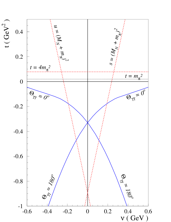
FIG. 2.: The Mandelstam plane for virtual Compton scattering at $Q^{2}$ = 0.33 GeV². The boundaries of the physical $s$-channel region are $\Theta_{\gamma\gamma}=0^{o}$ and $\Theta_{\gamma\gamma}=180^{o}$ for $\nu>0$, the $u$-channel region is obtained by crossing, $\nu\to-\nu$. The curves for $\Theta_{\gamma\gamma}=0^{o}$ and $\Theta_{\gamma\gamma}=180^{o}$ intersect at $\nu=0$, $t=-Q^{2}$, which is the point where the generalized polarizabilities are defined.

FIG. 3.: Results for the spin-flip GPs excluding the $\pi^{0}$-pole contribution in different model calculations, as function of the squared momentum transfer. The full curves correspond to the dispersive $\pi N$ contribution. The dashed curves show the results of ${\cal O}(p^{3})$ HBChPT [23], the dashed-dotted curves correspond to the predictions of the linear $\sigma$-model [24], and the dotted curves are the results of the nonrelativistic constituent quark model [25]. Note that the constituent quark model (CQM) results for $P^{(01,01)1}$ and $P^{(11,02)1}$ are multiplied (for visibility) by a factor 100.

FIG. 4.: Results for the spin-flip GPs as function of the squared momentum transfer. The dashed curves correspond to the dispersive $\pi N$ contribution, the dotted curves show the $\pi^{0}$-pole contribution, and the full curves are the sum of the dispersive and $\pi^{0}$-pole contributions. For comparison, we also show the $\pi^{0}$-pole contribution when setting the $\pi^{0}\gamma^{*}\gamma$ form factor equal to 1 (dashed-dotted curves). Note that $P^{(01,01)1}$ has no $\pi^{0}$-pole contribution.

FIG. 5.: Theoretical estimates of the asymptotic contribution $F_{1}^{as}$ : DR calculation [9] of the $\gamma^{*}\gamma\to\pi\pi\to N\bar{N}$ process as described in the text in Sec. VI B (full curve); linear $\sigma$-model (LSM) calculation [24] with $m_{\sigma}$ = 0.5 GeV (dotted curve) and $m_{\sigma}$ = 0.7 GeV (dashed-dotted curve). The dashed curves are dipole parametrizations according to Eq. (68), which are fixed to the phenomenological value at $Q^{2}$ = 0 and are shown for two values of the mass-scale, $\Lambda_{\beta}$ = 0.4 GeV (upper dashed curve, nearly coinciding with full curve) and $\Lambda_{\beta}$ = 0.6 GeV (lower dashed curve).

FIG. 6.: Results for the unpolarized structure functions $P_{LL}-P_{TT}/\varepsilon$ (upper panels), and $P_{LT}$ (lower panels), for $\varepsilon$ = 0.62. In the upper left panel, a comparison is shown between the dispersive $\pi N$ contribution of the GP $\alpha$ (full curve), the dispersive $\pi N$ contribution of the spin-flip GPs (dashed curve), and the asymptotic contribution of $\alpha$ according to Eq. (79) with $\Lambda_{\alpha}=1$ GeV (dotted curve). The upper right panel displays the total result for $P_{LL}-P_{TT}/\varepsilon$ (sum of the three contributions on the upper left panel) for $\Lambda_{\alpha}=1$ GeV (full curve) and $\Lambda_{\alpha}=1.4$ GeV (dashed curve). In the lower left panel, a comparison is shown between the dispersive $\pi N$ contribution of the GP $\beta$ (full curve), the contribution of the spin-flip GPs (dashed curve), and the asymptotic contribution of $\beta$ according to Eq. (68) with $\Lambda_{\beta}=0.6$ GeV (dotted curve). The lower right panel displays the total result for $P_{LT}$, for $\Lambda_{\beta}=0.7$ GeV (dotted curve), $\Lambda_{\beta}=0.6$ GeV (full curve), and $\Lambda_{\beta}=0.4$ GeV (dashed curve). The RCS data are from Ref. [27], and the VCS data at $Q^{2}=0.33\mbox{\, GeV}^{2}$ from Ref. [4].

FIG. 7.: $(d^{5}\sigma-d^{5}\sigma^{{\rm BH+Born}})/\Phi{\hbox{\rm q}^{\prime}}$ for the $ep\to ep\gamma$ reaction as function of the outgoing-photon energy ${\hbox{\rm q}^{\prime}}$ in MAMI kinematics : $\varepsilon=0.62$, ${\hbox{\rm q}}=0.6$ GeV, and for different photon c.m. angles $\Theta_{\gamma\gamma}^{c.m.}$. The data and the shaded bands, representing the best fit to the data within the LEX formalism, are from Ref. [4]. The solid curves are the DR results taking into account the full ${\hbox{\rm q}^{\prime}}$ dependence of the non-Born contribution to the cross section. The asymptotic contributions are calculated according to Eqs. (68, 79), with $\Lambda_{\beta}=0.6$ GeV and $\Lambda_{\alpha}=1$ GeV, respectively.

FIG. 8.: Upper panel: The differential cross section for the reaction $ep\to ep\gamma$ as function of the outgoing-photon energy ${\hbox{\rm q}^{\prime}}$ in MAMI kinematics : $\varepsilon=0.62$, ${\hbox{\rm q}}=0.6$ GeV, and for $\Theta_{\gamma\gamma}^{c.m.}=0^{\rm o}$, in plane ($\phi=0^{\rm o}$). The BH + Born contribution is given by the dashed-dotted curve. The total DR results are obtained with the asymptotic parts of Eqs. (68, 79), using a fixed value of $\Lambda_{\alpha}=1$ GeV and for the three values of $\Lambda_{\beta}$ as displayed in the lower right plot of Fig. 6, i.e. $\Lambda_{\beta}=0.7$ GeV (dotted curve), $\Lambda_{\beta}=0.6$ GeV (solid curve), and $\Lambda_{\beta}=0.4$ GeV (dashed curve). Lower panel: Results for $(d^{5}\sigma-d^{5}\sigma^{{\rm BH+Born}})/\Phi{\hbox{\rm q}^{\prime}}$ as function of ${\hbox{\rm q}^{\prime}}$ . The DR calculation taking into account the full energy dependence of the non-Born contribution (thick curves) are compared to the corresponding results within the LEX formalism (thin horizontal curves). The curves in the lower panel correspond to the same values of $\Lambda_{\alpha}$ and $\Lambda_{\beta}$ as in the upper panel. The data are from Ref. [4].

FIG. 9.: Same as Fig. 8 but for $\varepsilon$ = 0.8.

FIG. 10.: Left panels : The differential cross section for the reaction $ep\to ep\gamma$ as function of the photon scattering angle and at different values of the outgoing-photon energy ${\hbox{\rm q}^{\prime}}$ in JLab kinematics. Right panels : ratio of cross sections $(d\sigma-d\sigma^{BH+Born})/d\sigma^{BH+Born}$. Dashed-dotted curves on the left panels : BH+Born contribution. The DR results are displayed (on both left and right panels) with the asymptotic terms parametrized as in Eqs. (79, 68), using the values : $\Lambda_{\alpha}$ = 1 GeV and $\Lambda_{\beta}$ = 0.6 GeV (full curves), $\Lambda_{\alpha}$ = 1 GeV and $\Lambda_{\beta}$ = 0.4 GeV (dashed curves), $\Lambda_{\alpha}$ = 1.4 GeV and $\Lambda_{\beta}$ = 0.6 GeV (dotted curves).

FIG. 11.: $(d^{5}\sigma-d^{5}\sigma^{{\rm BH+Born}})/\Phi{\hbox{\rm q}^{\prime}}$ for the $ep\to ep\gamma$ reaction as function of the scattering angle and at different values of the outgoing-photon energy ${\hbox{\rm q}^{\prime}}$ in JLab kinematics. The solid curves correspond to the DR calculation with the full energy dependence of the non-Born contribution to the cross section. The dashed-dotted curves are the corresponding results obtained from the LEX. The asymptotic contributions have been calculated with the parametrizations in Eqs. (79, 68), using $\Lambda_{\alpha}=1.4$ GeV and $\Lambda_{\beta}=0.6$ GeV .

FIG. 12.: Upper panel: The differential cross sections for the $ep\to ep\gamma$ reaction as function of the c.m. energy W in JLab kinematics : $\varepsilon=0.95$, $Q^{2}=1$ GeV², and for fixed scattering angle $\Theta_{\gamma\gamma}^{c.m.}=-160^{\rm o}$, in plane ($\phi=0^{\rm o}$). The BH + Born contribution is given by the dashed-dotted curve. The total result including the non-Born contribution is shown for $\Lambda_{\beta}=0.6$ GeV and for the two values : $\Lambda_{\alpha}=1$ GeV (full curve), and $\Lambda_{\alpha}=1.4$ GeV (dashed curve). Lower panel: results for $(d^{5}\sigma-d^{5}\sigma^{{\rm BH+Born}})/\Phi{\hbox{\rm q}^{\prime}}$ as function of W. The curves in the lower panel correspond to the same values of $\Lambda_{\alpha}$ and $\Lambda_{\beta}$ as in the upper panel.

FIG. 13.: VCS double-polarization asymmetry (polarized electron, recoil proton polarization along either the $z$- or $x$- directions in the c.m. frame) in MAMI kinematics as function of the photon scattering angle. The dotted curves correspond to the BH+Born contribution. The dispersion results for the total BH+Born+non-Born cross section are shown for the values of the mass-scale $\Lambda_{\alpha}$ = 1 GeV, $\Lambda_{\beta}$ = 0.6 GeV (full curves) and $\Lambda_{\alpha}$ = 1 GeV, $\Lambda_{\beta}$ = 0.4 GeV (dashed curves). To see the effect of the $\pi^{0}$-pole contribution, we also show the results for the values $\Lambda_{\alpha}$ = 1 GeV, $\Lambda_{\beta}$ = 0.6 GeV, when turning off the $\pi^{0}$-pole contribution (dashed-dotted curves).

FIG. 14.: Upper panel : VCS double-polarization asymmetry (polarized electron, recoil proton polarization along the $z$-direction in the c.m. frame) in MAMI kinematics (same value of q and $\varepsilon$ as in Fig. 13) as function of the outgoing-photon energy at a fixed photon scattering angle $\Theta_{\gamma\gamma}^{c.m.}=-50^{\rm o}$, in plane ($\phi=0^{\rm o}$). The middle panel is the corresponding difference of polarized cross sections and the lower panel is the non-Born contribution to the corresponding polarized squared matrix element (according to Eq. (93)). The dotted curves correspond to the BH+Born contribution. The dispersion results for the total BH+Born+non-Born cross section (full curves) are calculated using the values $\Lambda_{\alpha}$ = 1 GeV and $\Lambda_{\beta}$ = 0.6 GeV. The dashed curves are the corresponding results obtained from the LEX. To see the effect of the $\pi^{0}$-pole contribution, we also show the results of the dispersion calculation, when turning off the $\pi^{0}$-pole contribution (dashed-dotted curves).

FIG. 15.: Electron single spin asymmetry (SSA) for VCS at $Q^{2}=0.12$ GeV², for two kinematics in the $\Delta(1232)$ region : W = 1.232 GeV, $\varepsilon=0.75$ (upper plots) and W = 1.17 GeV, $\varepsilon=0.81$ (lower plots). In both cases the SSA is shown as function of the photon scattering angle for two out-of-plane angles $\Phi$, as accessible at MIT-Bates [36]. The full dispersion results are shown for the values : $\Lambda_{\alpha}$ = 1 GeV, $\Lambda_{\beta}$ = 0.6 GeV (full curves), $\Lambda_{\alpha}$ = 1 GeV, $\Lambda_{\beta}$ = 0.4 GeV (dashed curves), and $\Lambda_{\alpha}$ = 1.4 GeV, $\Lambda_{\beta}$ = 0.6 GeV (dotted curves).

REFERENCES

- [1] P.A.M. Guichon and M. Vanderhaeghen, Prog. Part. Nucl. Phys. 41, 125 (1998).
- [2] M. Vanderhaeghen, Eur. Phys. J. A 8, 455 (2000).
- [3] P.A.M. Guichon, G.Q. Liu, and A.W. Thomas, Nucl. Phys. A591, 606 (1995).
- [4] J. Roche et al., Phys. Rev. Lett. 85, 708 (2000).
- [5] P.Y. Bertin, P.A.M. Guichon, and C. Hyde-Wright, spokespersons JLab experiment, E-93-050.
- [6] J. Shaw and R. Miskimen, spokespersons MIT-Bates experiment, 97-03.
- [7] N. d’Hose and H. Merkel, spokespersons MAMI experiment, (2001).
- [8] A. L’vov, V.A. Petrun’kin, and M. Schumacher, Phys. Rev. C 55, 359 (1997).
- [9] D. Drechsel, M. Gorchtein, B. Pasquini, and M. Vanderhaeghen, Phys. Rev. C 61, 015204 (1999).
- [10] B. Pasquini, D. Drechsel, M. Gorchtein, A. Metz, and M. Vanderhaeghen, Phys. Rev. C 62, 052201 (2000).
- [11] D. Drechsel, G. Knöchlein, A.Yu. Korchin, A. Metz, and S. Scherer, Phys. Rev. C 57, 941 (1998); Phys. Rev. C 58, 1751 (1998).
- [12] M. Vanderhaeghen, Phys. Lett. B 402, 243 (1997).
- [13] J.D. Bjorken and S.D. Drell, Relativistic Quantum Fields, McGraw-Hill, New York (1965).
- [14] H. Pilkuhn, Relativistic Particle Physics, Springer Verlag, Heidelberg (1979).
- [15] R.L. Jaffe and P.F. Mende, Nucl. Phys. B369, 189 (1992).
- [16] R. Oehme, Int. J. Phys. A 10, 1995 (1995).
- [17] R.A. Berg and C.N. Lindner, Nucl. Phys. 26, 259 (1961).
- [18] R. Tarrach, Nuovo Cimento A 28, 409 (1975).
- [19] D. Drechsel, G. Knöchlein, A. Metz, and S. Scherer, Phys. Rev. C 55, 424 (1997).
- [20] D. Drechsel, O. Hanstein, S. Kamalov, and L. Tiator, Nucl. Phys. A645, 145 (1999).
- [21] M.M. Pavan, R.A. Arndt, I.I. Strakovsky, and R.L. Workman, PiN Newslett. 15, 171 (1999).
- [22] S.J. Brodsky and G.P. Lepage, Phys. Rev. D 24, 1808 (1981).
- [23] T.R. Hemmert, B.R. Holstein, G. Knöchlein, and D. Drechsel, Phys. Rev. D 62, 014013 (2000).
- [24] A. Metz and D. Drechsel, Z. Phys. A356, 351 (1996); Z. Phys. A359, 165 (1997).
- [25] B. Pasquini, S. Scherer, and D. Drechsel, Phys. Rev. C 63, 025205 (2001).
- [26] D. Babusci, G. Giordano, and G. Matone, Phys. Rev. C 57, 291 (1998).
- [27] V. Olmos de León, et al., submitted to Eur. Phys. J. A.
- [28] G. Höhler, Pion-Nucleon Scattering, Landolt-Börnstein, Vol. I/9b2, edited by H. Schopper (Springer, Berlin, 1983).
- [29] B.R. Holstein and A.M. Nathan, Phys. Rev. D 49, 6101 (1994).
- [30] G. Höhler, E. Pietarinen, I. Sabba-Stefanescu, F. Borkowski, G.G. Simon, V.H. Walther, and R.D. Wendling, Nucl. Phys. B 114, 505 (1976).
- [31] N. Degrande, Ph.D. thesis, University Gent, (2001); Luc Van Hoorebeke, private communication.
- [32] S. Jaminion, Ph.D. thesis, Université Blaise Pascal, Clermont Ferrand, (2000); H. Fonvieille, private communication.
- [33] G. Laveissiere, private communication.
- [34] P.E. Bosted, Phys. Rev. C 51, 409 (1995).
- [35] M.K. Jones et al., Phys. Rev. Lett. 84, 1398 (2000).
- [36] N.I. Kaloskamis and C.N. Papanicolas, spokespersons MIT-Bates experiment, (1997).
- [37] J.D. Bjorken and S.D. Drell, Relativistic Quantum Mechanics, McGraw-Hill, New York (1964).
- [38] R.L. Walker, Phys. Rev. 182, 1729 (1969).