Non-Gaussian Correlations in the McLerran-Venugopalan Model

Abstract

We argue that the statistical weight function $W[\rho]$ appearing in the McLerran-Venugopalan model of a large nucleus is intrinsically non-Gaussian, even if we neglect quantum corrections. Based on the picture where the nucleus of radius $R$ consists of a collection of color-neutral nucleons, each of radius $a\ll R$, we show that to leading order in $\alpha_{s}$ and $a/R$ only the Gaussian part of $W[\rho]$ enters into the final expression for the gluon number density. Thus, the existing results in the literature which assume a Gaussian weight remain valid.

I Introduction

With the first collisions at the Brookhaven Relativistic Heavy Ion Collider, the experimental frontier in both energy and density has advanced. One of the goals of this machine is to search for the so-called quark-gluon plasma (QGP), a deconfined state of QCD where quarks and gluons form a sea of thermalized particles occupying a volume of space significantly larger than that of a typical hadron. Theoretically, whether and when this occurs depends on the initial conditions of the system. That is, what is the distribution of the quarks and gluons immediately before the nuclei collide?

One particularly fruitful approach to the determination of parton distribution functions in nuclei has been the McLerran-Venugopalan (MV) model[3, 4, 5]. The key observation underpinning the MV model is that for large enough nuclei and for small enough values of the longitudinal momentum fraction $x_{{}_{F}}$, a new hard scale $\kappa^{2}$, corresponding to the large color charge per unit transverse area, enters into the problem. Consequently, when $\kappa^{2}\gg\Lambda_{\rm QCD}^{2}$, it is argued that a classical treatment ought to provide a reasonable approximation to the gluon distribution. Three interrelated factors contribute to making the small-$x_{{}_{F}}$ region conducive to a classical description. First, a large number of color charges contribute to the source, implying that the vector potential takes on large values within the nucleus. Second, the large vector potential corresponds to the existence of a large number of gluons, inviting us to apply the Weiszäcker-Williams technique. And, third, the new large scale appears in the running strong coupling constant, $\alpha_{s}(\kappa^{2})$, which is small for sufficiently large $\kappa^{2}$. In the classical treatment advocated in Refs. [3, 4, 5], quantum mechanical expectation values are replaced by averages over a suitably chosen ensemble of color sources whose statistical weight function, $W[\rho]$, was argued to take on a Gaussian form.

Quantum corrections to the MV model were first computed in Ref. [6]: they were found to be large due to contributions of order $\alpha_{s}\ln(1/x_{{}_{F}})$. The subsequent re-examination of the foundations of the MV model performed in Ref. [7] led to the formulation of a set of renormalization group equations (RGE) describing the evolution of the weight function $W[\rho]$ as one changes the separation scale between hard and soft partons[8, 9, 10, 11, 12, 13, 14, 15, 16]. Early on in the development of the RGE it was conjectured [7, 8, 9] that the MV model could be viewed as an effective theory at small $x_{{}_{F}}$, with the effects of the quantum corrections absorbed into a renormalization of the weight function $W[\rho]$. This conjecture has recently been proven by the calculation in Ref. [14]. While explicit solutions to the evolution equations for $W[\rho]$ have not yet been obtained, it is known that a Gaussian distribution is not a solution to these equations[9].

While these developments were taking place, we set out to address a different issue, namely the poor infrared behavior of the correlation functions in the MV model. The two-point vector potential obtained in Ref. [7] grows like $(x^{2})^{x^{2}}$ at large distances ($x\gtrsim\Lambda_{\rm QCD}^{-1}$), signaling the onset of non-perturbative effects associated with confinement. In Ref. [17] we observed that since individual nucleons do not exhibit a net non-zero color charge, there should not be any long-range ($\gg\Lambda_{\rm QCD}^{-1}$) correlations between quarks. This requirement of color neutrality was cast into the form of a mathematical constraint on the two-point charge density correlation function. We found that the infrared divergence appearing in the MV model is completely absent when the color neutrality condition is enforced[17].

With the infrared divergences under control, it became clear that, at least in the classical treatment of Ref. [17], the $x_{{}_{F}}$ dependence of the gluon distribution remained trivial, with $x_{{}_{F}}dN/dx_{{}_{F}}$ independent of $x_{{}_{F}}$. There are two fairly obvious possible sources of non-trivial $x_{{}_{F}}$ dependence, depending on the value of $x_{{}_{F}}$ under consideration. First, we can imagine taking $x_{{}_{F}}$ to be somewhat larger than the values specified in the MV model. In this situation, the longitudinal resolution of the gluons becomes good enough to start to probe the longitudinal structure of the Lorentz-contracted nucleus which they see. This avenue of investigation was pursued in Ref. [18], where we developed a fully three-dimensional treatment of the classical gluon field of a large nucleus. Our view of the nucleus (radius $R$) as containing color-neutral nucleons (each of radius $a$) played a vital role in the calculation. Taking advantage of the smallness of the ratio $a/R$ for a large nucleus, and assuming that the nucleus possesses a spherically symmetric distribution of color charge in its rest frame, we found that the additional $x_{{}_{F}}$ dependence manifests itself by the appearance of the combination $\mathchoice{{\hbox{\boldmath$\displaystyle q$}}}{{\hbox{\boldmath$\textstyle q$}}}{{\hbox{\boldmath$\scriptstyle q$}}}{{\hbox{\boldmath$\scriptscriptstyle q$}}}^{2}{+}(x_{{}_{F}}m)^{2}$ in some (but not all) of the functions parametrizing the final result (see Eqs. (5.18)–(5.20) of Ref. [18]). Here $\textstyle q$ is the transverse momentum of the gluon and $m$ is the nucleon mass. Over most of the region where our extended treatment is valid, $(x_{{}_{F}}m)^{2}\ll\mathchoice{{\hbox{\boldmath$\displaystyle q$}}}{{\hbox{\boldmath$\textstyle q$}}}{{\hbox{\boldmath$\scriptstyle q$}}}{{\hbox{\boldmath$\scriptscriptstyle q$}}}^{2}$, implying that these corrections are small.

The second possible source of non-trivial $x_{{}_{F}}$ dependence, namely quantum corrections proportional to $\alpha_{s}\ln(1/x_{{}_{F}})$, was proposed [3, 4, 5] even before the first calculation of these corrections in Ref. [6] verified that they do indeed contain the necessary logarithms. The idea is that a resummation of such powers to all orders would convert the $1/x_{{}_{F}}$ appearing in the leading-order expression for $dN/dx_{{}_{F}}$ into $1/x_{{}_{F}}^{1+C\alpha_{s}}$ for some $C$. One of the goals of the studies conducted in Refs. [7, 8, 9, 10, 11, 12, 13, 14, 15, 16] may thus be phrased as the determination of $C$. A priori it would appear that in order to determine the gluon distribution in the interesting nonlinear regime, we would require a complete solution to the evolution equations for $W[\rho]$ developed in Refs. [7, 8, 9, 10, 11, 12, 13, 14, 15, 16]. And, furthermore, since a Gaussian is not a solution to these equations, it would seem that the general form of the gluon distribution obtained in Refs. [7, 17, 18] could be fundamentally altered once the non-Gaussian correlations are taken into account. Such an outcome would be at odds with related calculations based on different techniques [20, 21, 22, 23, 24, 25, 26, 27, 28, 29, 30, 31, 32, 33, 34, 35, 36, 37, 38, 39, 40, 41, 42, 43] which already possess general agreement with the MV model. The purpose of this paper is to investigate this issue. Once again it will prove valuable to incorporate the physics associated with confinement (i.e. the color neutrality of the nucleons) into the discussion. We will demonstrate that to leading order in the strong coupling and $a/R$ it is sufficient to consider only the (renormalized) Gaussian contributions to the gluon number density. All contributions from the non-Gaussian portion of $W[\rho]$ are suppressed by additional factors of $\alpha_{s}$ and/or $a/R$. Thus, the MV model remains in general agreement with the various other approaches to small-$x_{{}_{F}}$ physics referred to above, even if we employ a non-Gaussian weight function.

In light of the arguments in favor of a Gaussian form for $W[\rho]$ put forth in Ref. [3], the reader may be tempted to think that our conclusion is a trivial consequence of the central limit theorem. However, as we will demonstrate, the central limit theorem does not apply to this case. Instead, the additional factors which suppress the non-Gaussian terms relative to their Gaussian counterparts come about because of the fact that the individual nucleons are color neutral objects which do not have significant color-charge correlations at distances much greater than $a$.

The remainder of this paper is organized into two main sections. In the first, we begin with a review of the central limit theorem to establish the notation used in the subsequent discussion. We will pay particular attention to the conditions under which the central limit theorem is valid, and then show that for a large nucleus these conditions are violated. The essential observation is that any non-trivial longitudinal correlations, no matter how short range, spoil the Gaussian form of the weight function in the very large nucleus ($A^{1/3}\rightarrow\infty$) limit. In the second half of this paper we will return to the three-dimensional framework for the MV model developed in Ref. [18] and consider the additional terms which would be generated in the presence of non-Gaussian contributions to $W[\rho]$. Assuming only that the nucleus consists of color-neutral nucleons of radius $a$ which possess no nontrivial correlations at separations much larger than $a$, we will demonstrate that no contributions beyond those already considered in Refs. [7, 17, 18] are generated to leading order in $\alpha_{s}$ and $a/R$. Thus, for a large enough nucleus, it is sufficient to know only the two-point function associated with $W[\rho]$, even when the quantum corrections are taken into account. We close with a few words about the implications of our result.

II Gaussian and Non-Gaussian Distributions

A Gaussian (or Normal) distribution in a random variable $\textstyle t$ usually comes about because of the central limit theorem. In this section we review the conditions under which this theorem is valid, and argue that all of these conditions are not, in general, satisfied by the color-charge distribution of a large nucleus, even when we omit radiative corrections. Hence, the statistical weight function $W[\rho]$ appearing in the MV model is generically not expected to be a Gaussian, even classically.

A Generating Functions

Let $\textstyle\tau$ be a $D$-dimensional random variable, with normalized distribution $P(\mathchoice{{\hbox{\boldmath$\displaystyle\tau$}}}{{\hbox{\boldmath$\textstyle\tau$}}}{{\hbox{\boldmath$\scriptstyle\tau$}}}{{\hbox{\boldmath$\scriptscriptstyle\tau$}}})$. For what follows it is more convenient to specify it by its moments:

$$\langle\tau_{i}\tau_{j}\cdots\tau_{k}\rangle\equiv\int d^{D}\tau\ \tau_{i}\tau_{j}\cdots\tau_{k}\thinspace P(\mathchoice{{\hbox{\boldmath$\displaystyle\tau$}}}{{\hbox{\boldmath$\textstyle\tau$}}}{{\hbox{\boldmath$\scriptstyle\tau$}}}{{\hbox{\boldmath$\scriptscriptstyle\tau$}}}).$$ (1)

These two descriptions are equivalent because the Fourier transform of $P(\mathchoice{{\hbox{\boldmath$\displaystyle\tau$}}}{{\hbox{\boldmath$\textstyle\tau$}}}{{\hbox{\boldmath$\scriptstyle\tau$}}}{{\hbox{\boldmath$\scriptscriptstyle\tau$}}})$, namely

$$\widetilde{P}(\mathchoice{{\hbox{\boldmath$\displaystyle\lambda$}}}{{\hbox{\boldmath$\textstyle\lambda$}}}{{\hbox{\boldmath$\scriptstyle\lambda$}}}{{\hbox{\boldmath$\scriptscriptstyle\lambda$}}})=\int d^{D}\tau\thinspace e^{-i\mathchoice{{\hbox{\boldmath$\displaystyle\lambda$}}}{{\hbox{\boldmath$\textstyle\lambda$}}}{{\hbox{\boldmath$\scriptstyle\lambda$}}}{{\hbox{\boldmath$\scriptscriptstyle\lambda$}}}\,\!\cdot\!\,\mathchoice{{\hbox{\boldmath$\displaystyle\tau$}}}{{\hbox{\boldmath$\textstyle\tau$}}}{{\hbox{\boldmath$\scriptstyle\tau$}}}{{\hbox{\boldmath$\scriptscriptstyle\tau$}}}}P(\mathchoice{{\hbox{\boldmath$\displaystyle\tau$}}}{{\hbox{\boldmath$\textstyle\tau$}}}{{\hbox{\boldmath$\scriptstyle\tau$}}}{{\hbox{\boldmath$\scriptscriptstyle\tau$}}}),$$ (2)

has a Taylor series expansion in terms of the moments:

$$\widetilde{P}(\mathchoice{{\hbox{\boldmath$\displaystyle\lambda$}}}{{\hbox{\boldmath$\textstyle\lambda$}}}{{\hbox{\boldmath$\scriptstyle\lambda$}}}{{\hbox{\boldmath$\scriptscriptstyle\lambda$}}})=1+\sum_{n=1}^{\infty}{{(-i)^{n}}\over{n!}}\langle(\mathchoice{{\hbox{\boldmath$\displaystyle\tau$}}}{{\hbox{\boldmath$\textstyle\tau$}}}{{\hbox{\boldmath$\scriptstyle\tau$}}}{{\hbox{\boldmath$\scriptscriptstyle\tau$}}}\cdot\mathchoice{{\hbox{\boldmath$\displaystyle\lambda$}}}{{\hbox{\boldmath$\textstyle\lambda$}}}{{\hbox{\boldmath$\scriptstyle\lambda$}}}{{\hbox{\boldmath$\scriptscriptstyle\lambda$}}})^{n}\rangle.$$ (3)

The moments defined by Eq. (1) are reducible in the following sense. Suppose that the distribution $P(\mathchoice{{\hbox{\boldmath$\displaystyle\tau$}}}{{\hbox{\boldmath$\textstyle\tau$}}}{{\hbox{\boldmath$\scriptstyle\tau$}}}{{\hbox{\boldmath$\scriptscriptstyle\tau$}}})$ factorizes as

$$P(\mathchoice{{\hbox{\boldmath$\displaystyle\tau$}}}{{\hbox{\boldmath$\textstyle\tau$}}}{{\hbox{\boldmath$\scriptstyle\tau$}}}{{\hbox{\boldmath$\scriptscriptstyle\tau$}}})=\prod_{i=1}^{D}\thinspace p(\tau_{i}),$$ (4)

where $p(\tau_{i})$ is some single variable distribution, i.e. suppose that the components of the vector $\textstyle\tau$ are completely unrelated to each other. In this case, the moment $\langle\tau_{i}\tau_{j}\cdots\tau_{k}\rangle$ factorizes into $\langle\tau_{i}\rangle\langle\tau_{j}\rangle\cdots\langle\tau_{k}\rangle$. More generally, however, the components of $\textstyle\tau$ will not be completely independent of each other. Then, the factorization just described will fail: for example, $\langle\tau_{i}\tau_{j}\rangle\neq\langle\tau_{i}\rangle\langle\tau_{j}\rangle$. The difference between these two quantities provides a measure of the amount of interdependence between the components of $\textstyle\tau$. This information may be conveniently organized in terms of the (irreducible) cluster moments $\langle\!\langle\tau_{i}\tau_{j}\cdots\tau_{k}\rangle\!\rangle$, which are recursively defined through the relations

$$\langle\tau_{i}\rangle = \langle\!\langle\tau_{i}\rangle\!\rangle,$$ (6)

$$\langle\tau_{i}\tau_{j}\rangle = \langle\!\langle\tau_{i}\tau_{j}\rangle\!\rangle+\langle\!\langle\tau_{i}\rangle\!\rangle\langle\!\langle\tau_{j}\rangle\!\rangle,$$ (8)

$$\langle\tau_{i}\tau_{j}\tau_{k}\rangle = \langle\!\langle\tau_{i}\tau_{j}\tau_{k}\rangle\!\rangle+\langle\!\langle\tau_{i}\rangle\!\rangle\langle\!\langle\tau_{j}\tau_{k}\rangle\!\rangle+\langle\!\langle\tau_{j}\rangle\!\rangle\langle\!\langle\tau_{i}\tau_{k}\rangle\!\rangle+\langle\!\langle\tau_{k}\rangle\!\rangle\langle\!\langle\tau_{i}\tau_{j}\rangle\!\rangle+\langle\!\langle\tau_{i}\rangle\!\rangle\langle\!\langle\tau_{j}\rangle\!\rangle\langle\!\langle\tau_{k}\rangle\!\rangle,$$ (10)

$$\langle\tau_{i}\tau_{j}\tau_{k}\tau_{l}\rangle = \langle\!\langle\tau_{i}\tau_{j}\tau_{k}\tau_{l}\rangle\!\rangle$$ (12)

$$+\langle\!\langle\tau_{i}\rangle\!\rangle\langle\!\langle\tau_{j}\tau_{k}\tau_{l}\rangle\!\rangle+\langle\!\langle\tau_{j}\rangle\!\rangle\langle\!\langle\tau_{i}\tau_{k}\tau_{l}\rangle\!\rangle+\langle\!\langle\tau_{k}\rangle\!\rangle\langle\!\langle\tau_{i}\tau_{j}\tau_{l}\rangle\!\rangle+\langle\!\langle\tau_{l}\rangle\!\rangle\langle\!\langle\tau_{i}\tau_{j}\tau_{k}\rangle\!\rangle$$ (14)

$$+\langle\!\langle\tau_{i}\tau_{j}\rangle\!\rangle\langle\!\langle\tau_{k}\tau_{l}\rangle\!\rangle+\langle\!\langle\tau_{i}\tau_{k}\rangle\!\rangle\langle\!\langle\tau_{j}\tau_{l}\rangle\!\rangle+\langle\!\langle\tau_{i}\tau_{l}\rangle\!\rangle\langle\!\langle\tau_{j}\tau_{k}\rangle\!\rangle$$

$$+\langle\!\langle\tau_{i}\rangle\!\rangle\langle\!\langle\tau_{j}\rangle\!\rangle\langle\!\langle\tau_{k}\tau_{l}\rangle\!\rangle+\langle\!\langle\tau_{i}\rangle\!\rangle\langle\!\langle\tau_{k}\rangle\!\rangle\langle\!\langle\tau_{j}\tau_{l}\rangle\!\rangle+\langle\!\langle\tau_{i}\rangle\!\rangle\langle\!\langle\tau_{l}\rangle\!\rangle\langle\!\langle\tau_{j}\tau_{k}\rangle\!\rangle$$ (16)

$$+\langle\!\langle\tau_{j}\rangle\!\rangle\langle\!\langle\tau_{k}\rangle\!\rangle\langle\!\langle\tau_{i}\tau_{l}\rangle\!\rangle+\langle\!\langle\tau_{j}\rangle\!\rangle\langle\!\langle\tau_{l}\rangle\!\rangle\langle\!\langle\tau_{i}\tau_{k}\rangle\!\rangle+\langle\!\langle\tau_{k}\rangle\!\rangle\langle\!\langle\tau_{l}\rangle\!\rangle\langle\!\langle\tau_{i}\tau_{j}\rangle\!\rangle$$

$$+\langle\!\langle\tau_{i}\rangle\!\rangle\langle\!\langle\tau_{j}\rangle\!\rangle\langle\!\langle\tau_{k}\rangle\!\rangle\langle\!\langle\tau_{l}\rangle\!\rangle.$$ (17)

The generalization to higher orders is obvious. It turns out that the cluster moments are generated by $\ln\widetilde{P}(\mathchoice{{\hbox{\boldmath$\displaystyle\lambda$}}}{{\hbox{\boldmath$\textstyle\lambda$}}}{{\hbox{\boldmath$\scriptstyle\lambda$}}}{{\hbox{\boldmath$\scriptscriptstyle\lambda$}}})$, in the same way that the ordinary moments are generated by $\widetilde{P}(\mathchoice{{\hbox{\boldmath$\displaystyle\lambda$}}}{{\hbox{\boldmath$\textstyle\lambda$}}}{{\hbox{\boldmath$\scriptstyle\lambda$}}}{{\hbox{\boldmath$\scriptscriptstyle\lambda$}}})$:

$$\ln\widetilde{P}(\mathchoice{{\hbox{\boldmath$\displaystyle\lambda$}}}{{\hbox{\boldmath$\textstyle\lambda$}}}{{\hbox{\boldmath$\scriptstyle\lambda$}}}{{\hbox{\boldmath$\scriptscriptstyle\lambda$}}})=\sum_{n=1}^{\infty}{{(-i)^{n}}\over{n!}}\langle\!\langle(\mathchoice{{\hbox{\boldmath$\displaystyle\tau$}}}{{\hbox{\boldmath$\textstyle\tau$}}}{{\hbox{\boldmath$\scriptstyle\tau$}}}{{\hbox{\boldmath$\scriptscriptstyle\tau$}}}\cdot\mathchoice{{\hbox{\boldmath$\displaystyle\lambda$}}}{{\hbox{\boldmath$\textstyle\lambda$}}}{{\hbox{\boldmath$\scriptstyle\lambda$}}}{{\hbox{\boldmath$\scriptscriptstyle\lambda$}}})^{n}\rangle\!\rangle.$$ (18)

A simple example is provided by the following Gaussian distribution:

$$P(\mathchoice{{\hbox{\boldmath$\displaystyle\tau$}}}{{\hbox{\boldmath$\textstyle\tau$}}}{{\hbox{\boldmath$\scriptstyle\tau$}}}{{\hbox{\boldmath$\scriptscriptstyle\tau$}}})={{\exp(-\mathchoice{{\hbox{\boldmath$\displaystyle\tau$}}}{{\hbox{\boldmath$\textstyle\tau$}}}{{\hbox{\boldmath$\scriptstyle\tau$}}}{{\hbox{\boldmath$\scriptscriptstyle\tau$}}}^{2})}\over{{\pi}^{D/2}}}.$$ (19)

All of the odd moments (reducible and irreducible) of Eq. (19) vanish. Of the irreducible moments, only the two-point function $\langle\!\langle\tau_{i}\tau_{j}\rangle\!\rangle$ is nonvanishing. All other cluster moments are zero, and the even reducible moments are expressible entirely in terms $\langle\!\langle\tau_{i}\tau_{j}\rangle\!\rangle$.

B Central Limit Theorem

Suppose the random variable $\textstyle\tau$ is independently sampled $N$ times, yielding the values $\mathchoice{{\hbox{\boldmath$\displaystyle\tau$}}}{{\hbox{\boldmath$\textstyle\tau$}}}{{\hbox{\boldmath$\scriptstyle\tau$}}}{{\hbox{\boldmath$\scriptscriptstyle\tau$}}}^{(p)}\ (p=1,2,\ldots,N)$. The central limit theorem asserts that when $N\gg 1$, the mean value of these measurements,

$$\mathchoice{{\hbox{\boldmath$\displaystyle t$}}}{{\hbox{\boldmath$\textstyle t$}}}{{\hbox{\boldmath$\scriptstyle t$}}}{{\hbox{\boldmath$\scriptscriptstyle t$}}}\equiv{1\over N}\sum_{p=1}^{N}\mathchoice{{\hbox{\boldmath$\displaystyle\tau$}}}{{\hbox{\boldmath$\textstyle\tau$}}}{{\hbox{\boldmath$\scriptstyle\tau$}}}{{\hbox{\boldmath$\scriptscriptstyle\tau$}}}^{(p)},$$ (20)

obeys a Gaussian distribution with

$$\langle\!\langle t_{i}\rangle\!\rangle={\langle\!\langle\tau_{i}\rangle\!\rangle}=\langle\tau_{i}\rangle$$ (22)

and

$$\langle\!\langle t_{i}t_{j}\rangle\!\rangle={{\langle\!\langle\tau_{i}\tau_{j}\rangle\!\rangle}\over{N}}.$$ (23)

In other words, the distribution of $\textstyle t$ is given by

$$W(\mathchoice{{\hbox{\boldmath$\displaystyle t$}}}{{\hbox{\boldmath$\textstyle t$}}}{{\hbox{\boldmath$\scriptstyle t$}}}{{\hbox{\boldmath$\scriptscriptstyle t$}}})=\sqrt{{\det\Omega}\over{(2\pi)^{D}}}\thinspace\exp\left[-\hbox{$1\over 2$}(t_{i}-\langle\tau_{i}\rangle)\Omega_{ij}(t_{j}-\langle\tau_{j}\rangle)\right],$$ (24)

where

$$\left(\Omega^{-1}\right)_{ij}\equiv{{\langle\!\langle\tau_{i}\tau_{j}\rangle\!\rangle}\over{N}}.$$ (25)

The proof of the central limit theorem relies crucially on the independence of samplings: the joint distribution $Q$ of the sampled variables $\mathchoice{{\hbox{\boldmath$\displaystyle\tau$}}}{{\hbox{\boldmath$\textstyle\tau$}}}{{\hbox{\boldmath$\scriptstyle\tau$}}}{{\hbox{\boldmath$\scriptscriptstyle\tau$}}}^{(p)}$ must be factorizable, i.e.

$$Q(\mathchoice{{\hbox{\boldmath$\displaystyle\tau$}}}{{\hbox{\boldmath$\textstyle\tau$}}}{{\hbox{\boldmath$\scriptstyle\tau$}}}{{\hbox{\boldmath$\scriptscriptstyle\tau$}}}^{(1)},\mathchoice{{\hbox{\boldmath$\displaystyle\tau$}}}{{\hbox{\boldmath$\textstyle\tau$}}}{{\hbox{\boldmath$\scriptstyle\tau$}}}{{\hbox{\boldmath$\scriptscriptstyle\tau$}}}^{(2)},\ldots,\mathchoice{{\hbox{\boldmath$\displaystyle\tau$}}}{{\hbox{\boldmath$\textstyle\tau$}}}{{\hbox{\boldmath$\scriptstyle\tau$}}}{{\hbox{\boldmath$\scriptscriptstyle\tau$}}}^{(N)})=\prod_{p=1}^{N}P(\mathchoice{{\hbox{\boldmath$\displaystyle\tau$}}}{{\hbox{\boldmath$\textstyle\tau$}}}{{\hbox{\boldmath$\scriptstyle\tau$}}}{{\hbox{\boldmath$\scriptscriptstyle\tau$}}}^{(p)}).$$ (26)

In terms of $Q$, the probability $W(\mathchoice{{\hbox{\boldmath$\displaystyle t$}}}{{\hbox{\boldmath$\textstyle t$}}}{{\hbox{\boldmath$\scriptstyle t$}}}{{\hbox{\boldmath$\scriptscriptstyle t$}}})$ for finding the mean value $\textstyle t$ is given by

$$W(\mathchoice{{\hbox{\boldmath$\displaystyle t$}}}{{\hbox{\boldmath$\textstyle t$}}}{{\hbox{\boldmath$\scriptstyle t$}}}{{\hbox{\boldmath$\scriptscriptstyle t$}}})=\int d^{D}\mathchoice{{\hbox{\boldmath$\displaystyle\tau$}}}{{\hbox{\boldmath$\textstyle\tau$}}}{{\hbox{\boldmath$\scriptstyle\tau$}}}{{\hbox{\boldmath$\scriptscriptstyle\tau$}}}^{(1)}\int d^{D}\mathchoice{{\hbox{\boldmath$\displaystyle\tau$}}}{{\hbox{\boldmath$\textstyle\tau$}}}{{\hbox{\boldmath$\scriptstyle\tau$}}}{{\hbox{\boldmath$\scriptscriptstyle\tau$}}}^{(2)}\cdots\int d^{D}\mathchoice{{\hbox{\boldmath$\displaystyle\tau$}}}{{\hbox{\boldmath$\textstyle\tau$}}}{{\hbox{\boldmath$\scriptstyle\tau$}}}{{\hbox{\boldmath$\scriptscriptstyle\tau$}}}^{(N)}\thinspace Q(\mathchoice{{\hbox{\boldmath$\displaystyle\tau$}}}{{\hbox{\boldmath$\textstyle\tau$}}}{{\hbox{\boldmath$\scriptstyle\tau$}}}{{\hbox{\boldmath$\scriptscriptstyle\tau$}}}^{(1)},\mathchoice{{\hbox{\boldmath$\displaystyle\tau$}}}{{\hbox{\boldmath$\textstyle\tau$}}}{{\hbox{\boldmath$\scriptstyle\tau$}}}{{\hbox{\boldmath$\scriptscriptstyle\tau$}}}^{(2)},\ldots,\mathchoice{{\hbox{\boldmath$\displaystyle\tau$}}}{{\hbox{\boldmath$\textstyle\tau$}}}{{\hbox{\boldmath$\scriptstyle\tau$}}}{{\hbox{\boldmath$\scriptscriptstyle\tau$}}}^{(N)})\ \delta^{D}\biggl{(}\mathchoice{{\hbox{\boldmath$\displaystyle t$}}}{{\hbox{\boldmath$\textstyle t$}}}{{\hbox{\boldmath$\scriptstyle t$}}}{{\hbox{\boldmath$\scriptscriptstyle t$}}}-\sum_{p=1}^{N}\mathchoice{{\hbox{\boldmath$\displaystyle\tau$}}}{{\hbox{\boldmath$\textstyle\tau$}}}{{\hbox{\boldmath$\scriptstyle\tau$}}}{{\hbox{\boldmath$\scriptscriptstyle\tau$}}}^{(p)}/N\biggr{)}.$$ (27)

Using the distribution given in (26), the moment generating function is simply

$$\widetilde{W}(\mathchoice{{\hbox{\boldmath$\displaystyle\lambda$}}}{{\hbox{\boldmath$\textstyle\lambda$}}}{{\hbox{\boldmath$\scriptstyle\lambda$}}}{{\hbox{\boldmath$\scriptscriptstyle\lambda$}}}) = \int d^{D}\mathchoice{{\hbox{\boldmath$\displaystyle t$}}}{{\hbox{\boldmath$\textstyle t$}}}{{\hbox{\boldmath$\scriptstyle t$}}}{{\hbox{\boldmath$\scriptscriptstyle t$}}}\thinspace\thinspace e^{-i\mathchoice{{\hbox{\boldmath$\displaystyle\lambda$}}}{{\hbox{\boldmath$\textstyle\lambda$}}}{{\hbox{\boldmath$\scriptstyle\lambda$}}}{{\hbox{\boldmath$\scriptscriptstyle\lambda$}}}\cdot\mathchoice{{\hbox{\boldmath$\displaystyle t$}}}{{\hbox{\boldmath$\textstyle t$}}}{{\hbox{\boldmath$\scriptstyle t$}}}{{\hbox{\boldmath$\scriptscriptstyle t$}}}}\thinspace W(\mathchoice{{\hbox{\boldmath$\displaystyle t$}}}{{\hbox{\boldmath$\textstyle t$}}}{{\hbox{\boldmath$\scriptstyle t$}}}{{\hbox{\boldmath$\scriptscriptstyle t$}}})$$ (28)

$$= \left[\widetilde{P}\left({\mathchoice{{\hbox{\boldmath$\displaystyle\lambda$}}}{{\hbox{\boldmath$\textstyle\lambda$}}}{{\hbox{\boldmath$\scriptstyle\lambda$}}}{{\hbox{\boldmath$\scriptscriptstyle\lambda$}}}/N}\right)\right]^{N}.$$ (29)

This leads to the cluster moment generating function

$$\ln\widetilde{W}(\mathchoice{{\hbox{\boldmath$\displaystyle\lambda$}}}{{\hbox{\boldmath$\textstyle\lambda$}}}{{\hbox{\boldmath$\scriptstyle\lambda$}}}{{\hbox{\boldmath$\scriptscriptstyle\lambda$}}}) = N\ln\widetilde{P}\left({\mathchoice{{\hbox{\boldmath$\displaystyle\lambda$}}}{{\hbox{\boldmath$\textstyle\lambda$}}}{{\hbox{\boldmath$\scriptstyle\lambda$}}}{{\hbox{\boldmath$\scriptscriptstyle\lambda$}}}/N}\right)$$ (30)

$$= \sum_{n=1}^{\infty}{{(-i)^{n}}\over{n!}}{{\langle\!\langle(\mathchoice{{\hbox{\boldmath$\displaystyle\tau$}}}{{\hbox{\boldmath$\textstyle\tau$}}}{{\hbox{\boldmath$\scriptstyle\tau$}}}{{\hbox{\boldmath$\scriptscriptstyle\tau$}}}\!\cdot\!\mathchoice{{\hbox{\boldmath$\displaystyle\lambda$}}}{{\hbox{\boldmath$\textstyle\lambda$}}}{{\hbox{\boldmath$\scriptstyle\lambda$}}}{{\hbox{\boldmath$\scriptscriptstyle\lambda$}}})^{n}\rangle\!\rangle}\over{\thinspace N^{n-1}}},$$ (31)

where we have applied Eq. (18) to obtain the second line. Now consider the $N\gg 1$ limit. If we approximate (31) by just the first term, we obtain $W(\mathchoice{{\hbox{\boldmath$\displaystyle\lambda$}}}{{\hbox{\boldmath$\textstyle\lambda$}}}{{\hbox{\boldmath$\scriptstyle\lambda$}}}{{\hbox{\boldmath$\scriptscriptstyle\lambda$}}})=\exp(-i\mathchoice{{\hbox{\boldmath$\displaystyle\lambda$}}}{{\hbox{\boldmath$\textstyle\lambda$}}}{{\hbox{\boldmath$\scriptstyle\lambda$}}}{{\hbox{\boldmath$\scriptscriptstyle\lambda$}}}\cdot\langle\mathchoice{{\hbox{\boldmath$\displaystyle\tau$}}}{{\hbox{\boldmath$\textstyle\tau$}}}{{\hbox{\boldmath$\scriptstyle\tau$}}}{{\hbox{\boldmath$\scriptscriptstyle\tau$}}}\rangle)$, corresponding to $W(\mathchoice{{\hbox{\boldmath$\displaystyle t$}}}{{\hbox{\boldmath$\textstyle t$}}}{{\hbox{\boldmath$\scriptstyle t$}}}{{\hbox{\boldmath$\scriptscriptstyle t$}}})=\delta^{D}(\mathchoice{{\hbox{\boldmath$\displaystyle t$}}}{{\hbox{\boldmath$\textstyle t$}}}{{\hbox{\boldmath$\scriptstyle t$}}}{{\hbox{\boldmath$\scriptscriptstyle t$}}}-\langle\mathchoice{{\hbox{\boldmath$\displaystyle\tau$}}}{{\hbox{\boldmath$\textstyle\tau$}}}{{\hbox{\boldmath$\scriptstyle\tau$}}}{{\hbox{\boldmath$\scriptscriptstyle\tau$}}}\rangle)$. If instead, we include the first two terms in the infinite series, we get

$$\widetilde{W}(\mathchoice{{\hbox{\boldmath$\displaystyle\lambda$}}}{{\hbox{\boldmath$\textstyle\lambda$}}}{{\hbox{\boldmath$\scriptstyle\lambda$}}}{{\hbox{\boldmath$\scriptscriptstyle\lambda$}}})=\exp\Bigl{(}-i\mathchoice{{\hbox{\boldmath$\displaystyle\lambda$}}}{{\hbox{\boldmath$\textstyle\lambda$}}}{{\hbox{\boldmath$\scriptstyle\lambda$}}}{{\hbox{\boldmath$\scriptscriptstyle\lambda$}}}\!\cdot\!\langle\mathchoice{{\hbox{\boldmath$\displaystyle\tau$}}}{{\hbox{\boldmath$\textstyle\tau$}}}{{\hbox{\boldmath$\scriptstyle\tau$}}}{{\hbox{\boldmath$\scriptscriptstyle\tau$}}}\rangle-\lambda_{i}\lambda_{j}\langle\!\langle\tau_{i}\tau_{j}\rangle\!\rangle/2N\Bigr{)},$$ (32)

corresponding to the Gaussian distribution (24). Deviations from this Gaussian are suppressed by the additional powers of $1/N$ present in the higher order terms.

C Non-Gaussian Distribution

The proof of the central limit theorem depends critically on the assumption of independent sampling. If (26) is violated, then the proof fails. Even a small correlation between successive samplings is sufficient to destroy the conclusion, as the following example illustrates.

Suppose we introduce a “nearest-neighbor” correlation by replacing (26) with

$$Q(\mathchoice{{\hbox{\boldmath$\displaystyle\tau$}}}{{\hbox{\boldmath$\textstyle\tau$}}}{{\hbox{\boldmath$\scriptstyle\tau$}}}{{\hbox{\boldmath$\scriptscriptstyle\tau$}}}^{(1)},\mathchoice{{\hbox{\boldmath$\displaystyle\tau$}}}{{\hbox{\boldmath$\textstyle\tau$}}}{{\hbox{\boldmath$\scriptstyle\tau$}}}{{\hbox{\boldmath$\scriptscriptstyle\tau$}}}^{(2)},\ldots,\mathchoice{{\hbox{\boldmath$\displaystyle\tau$}}}{{\hbox{\boldmath$\textstyle\tau$}}}{{\hbox{\boldmath$\scriptstyle\tau$}}}{{\hbox{\boldmath$\scriptscriptstyle\tau$}}}^{(N)})=\Biggl{[}1+\sum_{m=1}^{N-1}{{f(\mathchoice{{\hbox{\boldmath$\displaystyle\tau$}}}{{\hbox{\boldmath$\textstyle\tau$}}}{{\hbox{\boldmath$\scriptstyle\tau$}}}{{\hbox{\boldmath$\scriptscriptstyle\tau$}}}^{(m)},\mathchoice{{\hbox{\boldmath$\displaystyle\tau$}}}{{\hbox{\boldmath$\textstyle\tau$}}}{{\hbox{\boldmath$\scriptstyle\tau$}}}{{\hbox{\boldmath$\scriptscriptstyle\tau$}}}^{(m+1)})}\over{P(\mathchoice{{\hbox{\boldmath$\displaystyle\tau$}}}{{\hbox{\boldmath$\textstyle\tau$}}}{{\hbox{\boldmath$\scriptstyle\tau$}}}{{\hbox{\boldmath$\scriptscriptstyle\tau$}}}^{(m)})\thinspace P(\mathchoice{{\hbox{\boldmath$\displaystyle\tau$}}}{{\hbox{\boldmath$\textstyle\tau$}}}{{\hbox{\boldmath$\scriptstyle\tau$}}}{{\hbox{\boldmath$\scriptscriptstyle\tau$}}}^{(m+1)})}}\Biggr{]}\prod_{p=1}^{N}P(\mathchoice{{\hbox{\boldmath$\displaystyle\tau$}}}{{\hbox{\boldmath$\textstyle\tau$}}}{{\hbox{\boldmath$\scriptstyle\tau$}}}{{\hbox{\boldmath$\scriptscriptstyle\tau$}}}^{(p)}).$$ (33)

To ensure that (33) is properly normalized, we further assume $f(\mathchoice{{\hbox{\boldmath$\displaystyle\tau$}}}{{\hbox{\boldmath$\textstyle\tau$}}}{{\hbox{\boldmath$\scriptstyle\tau$}}}{{\hbox{\boldmath$\scriptscriptstyle\tau$}}}^{(m)},\mathchoice{{\hbox{\boldmath$\displaystyle\tau$}}}{{\hbox{\boldmath$\textstyle\tau$}}}{{\hbox{\boldmath$\scriptstyle\tau$}}}{{\hbox{\boldmath$\scriptscriptstyle\tau$}}}^{(m+1)})$ to be symmetric in its arguments, and that

$$\int d^{D}\mathchoice{{\hbox{\boldmath$\displaystyle\tau$}}}{{\hbox{\boldmath$\textstyle\tau$}}}{{\hbox{\boldmath$\scriptstyle\tau$}}}{{\hbox{\boldmath$\scriptscriptstyle\tau$}}}^{(m)}f(\mathchoice{{\hbox{\boldmath$\displaystyle\tau$}}}{{\hbox{\boldmath$\textstyle\tau$}}}{{\hbox{\boldmath$\scriptstyle\tau$}}}{{\hbox{\boldmath$\scriptscriptstyle\tau$}}}^{(m)},\mathchoice{{\hbox{\boldmath$\displaystyle\tau$}}}{{\hbox{\boldmath$\textstyle\tau$}}}{{\hbox{\boldmath$\scriptstyle\tau$}}}{{\hbox{\boldmath$\scriptscriptstyle\tau$}}}^{(m+1)})=0.$$ (34)

The moment generating function for the distribution (27) is now

$$\widetilde{W}(\mathchoice{{\hbox{\boldmath$\displaystyle\lambda$}}}{{\hbox{\boldmath$\textstyle\lambda$}}}{{\hbox{\boldmath$\scriptstyle\lambda$}}}{{\hbox{\boldmath$\scriptscriptstyle\lambda$}}})=\Bigl{[}{\widetilde{P}}(\mathchoice{{\hbox{\boldmath$\displaystyle\lambda$}}}{{\hbox{\boldmath$\textstyle\lambda$}}}{{\hbox{\boldmath$\scriptstyle\lambda$}}}{{\hbox{\boldmath$\scriptscriptstyle\lambda$}}}/N)\Bigr{]}^{N}\left\{1+{{{(N-1)\widetilde{f}(\mathchoice{{\hbox{\boldmath$\displaystyle\lambda$}}}{{\hbox{\boldmath$\textstyle\lambda$}}}{{\hbox{\boldmath$\scriptstyle\lambda$}}}{{\hbox{\boldmath$\scriptscriptstyle\lambda$}}})}\over{\Bigl{[}{\widetilde{P}}(\mathchoice{{\hbox{\boldmath$\displaystyle\lambda$}}}{{\hbox{\boldmath$\textstyle\lambda$}}}{{\hbox{\boldmath$\scriptstyle\lambda$}}}{{\hbox{\boldmath$\scriptscriptstyle\lambda$}}}/N)\Bigr{]}^{2}}}}\right\},$$ (35)

where

$$\widetilde{f}(\mathchoice{{\hbox{\boldmath$\displaystyle\lambda$}}}{{\hbox{\boldmath$\textstyle\lambda$}}}{{\hbox{\boldmath$\scriptstyle\lambda$}}}{{\hbox{\boldmath$\scriptscriptstyle\lambda$}}})\equiv\int d^{D}\mathchoice{{\hbox{\boldmath$\displaystyle\tau$}}}{{\hbox{\boldmath$\textstyle\tau$}}}{{\hbox{\boldmath$\scriptstyle\tau$}}}{{\hbox{\boldmath$\scriptscriptstyle\tau$}}}^{(1)}\int d^{D}\mathchoice{{\hbox{\boldmath$\displaystyle\tau$}}}{{\hbox{\boldmath$\textstyle\tau$}}}{{\hbox{\boldmath$\scriptstyle\tau$}}}{{\hbox{\boldmath$\scriptscriptstyle\tau$}}}^{(2)}\thinspace e^{-i\mathchoice{{\hbox{\boldmath$\displaystyle\lambda$}}}{{\hbox{\boldmath$\textstyle\lambda$}}}{{\hbox{\boldmath$\scriptstyle\lambda$}}}{{\hbox{\boldmath$\scriptscriptstyle\lambda$}}}\cdot[\mathchoice{{\hbox{\boldmath$\displaystyle\tau$}}}{{\hbox{\boldmath$\textstyle\tau$}}}{{\hbox{\boldmath$\scriptstyle\tau$}}}{{\hbox{\boldmath$\scriptscriptstyle\tau$}}}^{(1)}+\mathchoice{{\hbox{\boldmath$\displaystyle\tau$}}}{{\hbox{\boldmath$\textstyle\tau$}}}{{\hbox{\boldmath$\scriptstyle\tau$}}}{{\hbox{\boldmath$\scriptscriptstyle\tau$}}}^{(2)}]}\thinspace f(\mathchoice{{\hbox{\boldmath$\displaystyle\tau$}}}{{\hbox{\boldmath$\textstyle\tau$}}}{{\hbox{\boldmath$\scriptstyle\tau$}}}{{\hbox{\boldmath$\scriptscriptstyle\tau$}}}^{(1)},\mathchoice{{\hbox{\boldmath$\displaystyle\tau$}}}{{\hbox{\boldmath$\textstyle\tau$}}}{{\hbox{\boldmath$\scriptstyle\tau$}}}{{\hbox{\boldmath$\scriptscriptstyle\tau$}}}^{(2)}).$$ (36)

Note that $\widetilde{f}(\mathchoice{{\hbox{\boldmath$\displaystyle 0$}}}{{\hbox{\boldmath$\textstyle 0$}}}{{\hbox{\boldmath$\scriptstyle 0$}}}{{\hbox{\boldmath$\scriptscriptstyle 0$}}})=0$. Unlike Eq. (31), the irreducible moments generated by

$$\ln\widetilde{W}(\mathchoice{{\hbox{\boldmath$\displaystyle\lambda$}}}{{\hbox{\boldmath$\textstyle\lambda$}}}{{\hbox{\boldmath$\scriptstyle\lambda$}}}{{\hbox{\boldmath$\scriptscriptstyle\lambda$}}})=N\ln\widetilde{P}(\mathchoice{{\hbox{\boldmath$\displaystyle\lambda$}}}{{\hbox{\boldmath$\textstyle\lambda$}}}{{\hbox{\boldmath$\scriptstyle\lambda$}}}{{\hbox{\boldmath$\scriptscriptstyle\lambda$}}}/N)+\ln\left\{1+{{{(N-1)\widetilde{f}(\mathchoice{{\hbox{\boldmath$\displaystyle\lambda$}}}{{\hbox{\boldmath$\textstyle\lambda$}}}{{\hbox{\boldmath$\scriptstyle\lambda$}}}{{\hbox{\boldmath$\scriptscriptstyle\lambda$}}}/N)}\over{\Bigl{[}{\widetilde{P}}(\mathchoice{{\hbox{\boldmath$\displaystyle\lambda$}}}{{\hbox{\boldmath$\textstyle\lambda$}}}{{\hbox{\boldmath$\scriptstyle\lambda$}}}{{\hbox{\boldmath$\scriptscriptstyle\lambda$}}}/N)\Bigr{]}^{2}}}}\right\}$$ (37)

do not approach a linear function of $\textstyle\lambda$ as $N\to\infty$. In fact, we have

$$\ln\widetilde{W}(\mathchoice{{\hbox{\boldmath$\displaystyle\lambda$}}}{{\hbox{\boldmath$\textstyle\lambda$}}}{{\hbox{\boldmath$\scriptstyle\lambda$}}}{{\hbox{\boldmath$\scriptscriptstyle\lambda$}}})=-i\mathchoice{{\hbox{\boldmath$\displaystyle\lambda$}}}{{\hbox{\boldmath$\textstyle\lambda$}}}{{\hbox{\boldmath$\scriptstyle\lambda$}}}{{\hbox{\boldmath$\scriptscriptstyle\lambda$}}}\!\cdot\!\langle\mathchoice{{\hbox{\boldmath$\displaystyle\tau$}}}{{\hbox{\boldmath$\textstyle\tau$}}}{{\hbox{\boldmath$\scriptstyle\tau$}}}{{\hbox{\boldmath$\scriptscriptstyle\tau$}}}\rangle+\ln\left[1-i\mathchoice{{\hbox{\boldmath$\displaystyle\lambda$}}}{{\hbox{\boldmath$\textstyle\lambda$}}}{{\hbox{\boldmath$\scriptstyle\lambda$}}}{{\hbox{\boldmath$\scriptscriptstyle\lambda$}}}\!\cdot\!\mathchoice{{\hbox{\boldmath$\displaystyle\phi$}}}{{\hbox{\boldmath$\textstyle\phi$}}}{{\hbox{\boldmath$\scriptstyle\phi$}}}{{\hbox{\boldmath$\scriptscriptstyle\phi$}}}\right]+{\cal O}(1/N),$$ (38)

where

$$\phi_{j}\equiv i{{\partial}\over{\partial\lambda_{j}}}\thinspace\widetilde{f}(\mathchoice{{\hbox{\boldmath$\displaystyle\lambda$}}}{{\hbox{\boldmath$\textstyle\lambda$}}}{{\hbox{\boldmath$\scriptstyle\lambda$}}}{{\hbox{\boldmath$\scriptscriptstyle\lambda$}}})\biggl{|}_{\lambda=0}.$$ (39)

For $\mathchoice{{\hbox{\boldmath$\displaystyle\phi$}}}{{\hbox{\boldmath$\textstyle\phi$}}}{{\hbox{\boldmath$\scriptstyle\phi$}}}{{\hbox{\boldmath$\scriptscriptstyle\phi$}}}\not=0$, Eq. (38) is nonlinear in $\textstyle\lambda$. This distribution possesses non-zero values for all of its irreducible moments, independent of $N$. Including the ${\cal O}(1/N)$ contributions does not change this conclusion. The corresponding distribution $W(\mathchoice{{\hbox{\boldmath$\displaystyle t$}}}{{\hbox{\boldmath$\textstyle t$}}}{{\hbox{\boldmath$\scriptstyle t$}}}{{\hbox{\boldmath$\scriptscriptstyle t$}}})$ is no longer a pure Gaussian: the central limit theorem does not hold in this case. While it is straightforward to determine the (new) form of the distribution function for this particular example, in general this task will not be so easy. Fortunately, all we need to know for what follows is the fact that the resulting distribution is fundamentally non-Gaussian when the successive measurements are (even mildly) correlated.

It is useful to see a bit more about how the correlators change when we relax the assumption of independent measurements. With independent sampling, as in Eq. (26), correlators such as $\langle\tau_{i}^{(p)}\tau_{j}^{(q)}\cdots\tau_{k}^{(s)}\rangle$ factorize into groups with the same superscripts. For example,

$$\langle\tau_{i}^{(p)}\tau_{j}^{(q)}\tau_{k}^{(s)}\tau_{l}^{(s)}\rangle = \int d^{D}\mathchoice{{\hbox{\boldmath$\displaystyle\tau$}}}{{\hbox{\boldmath$\textstyle\tau$}}}{{\hbox{\boldmath$\scriptstyle\tau$}}}{{\hbox{\boldmath$\scriptscriptstyle\tau$}}}^{(1)}\cdots\int d^{D}\mathchoice{{\hbox{\boldmath$\displaystyle\tau$}}}{{\hbox{\boldmath$\textstyle\tau$}}}{{\hbox{\boldmath$\scriptstyle\tau$}}}{{\hbox{\boldmath$\scriptscriptstyle\tau$}}}^{(N)}\thinspace\thinspace\tau_{i}^{(p)}\tau_{j}^{(q)}\tau_{k}^{(s)}\tau_{l}^{(s)}\thinspace P(\mathchoice{{\hbox{\boldmath$\displaystyle\tau$}}}{{\hbox{\boldmath$\textstyle\tau$}}}{{\hbox{\boldmath$\scriptstyle\tau$}}}{{\hbox{\boldmath$\scriptscriptstyle\tau$}}}^{(1)})\cdots P(\mathchoice{{\hbox{\boldmath$\displaystyle\tau$}}}{{\hbox{\boldmath$\textstyle\tau$}}}{{\hbox{\boldmath$\scriptstyle\tau$}}}{{\hbox{\boldmath$\scriptscriptstyle\tau$}}}^{(N)})$$ (40)

$$= \langle\tau_{i}\rangle\langle\tau_{j}\rangle\langle\tau_{k}\tau_{l}\rangle,$$ (41)

assuming that $p$, $q$, and $s$ all take on distinct values. Of particular interest in connection with the MV model will be the special case

$$\langle\tau_{i}^{(p)}\tau_{j}^{(q)}\rangle=\delta^{pq}\langle\tau_{i}\tau_{j}\rangle+(1-\delta^{pq})\langle\tau_{i}\rangle\langle\tau_{j}\rangle.$$ (42)

In contrast, if the measurements are not independent, such as in (33), then the factorizations obtained in Eqs. (41) and (42) are no longer valid. Additional non-factorizable correlators involving different superscripts will, in general, be present, signaling the breakdown of the central limit theorem.

D Color Charge Distribution in a Large Nucleus

Let $\rho^{a}(x_{\scriptscriptstyle\parallel},\mathchoice{{\hbox{\boldmath$\displaystyle x$}}}{{\hbox{\boldmath$\textstyle x$}}}{{\hbox{\boldmath$\scriptstyle x$}}}{{\hbox{\boldmath$\scriptscriptstyle x$}}})$ be the color charge density of a large nucleus with color $a$ and atomic weight $A\gg 1$, at the transverse position $\textstyle x$ and the longitudinal position $x_{\scriptscriptstyle\parallel}$ (a precise definition of $x_{\scriptscriptstyle\parallel}$ is given in Eq. (49) below). Let

$$\rho^{a}_{2}(\mathchoice{{\hbox{\boldmath$\displaystyle x$}}}{{\hbox{\boldmath$\textstyle x$}}}{{\hbox{\boldmath$\scriptstyle x$}}}{{\hbox{\boldmath$\scriptscriptstyle x$}}})\equiv\int_{-\infty}^{\infty}dx_{\scriptscriptstyle\parallel}\thinspace\rho^{a}(x_{\scriptscriptstyle\parallel},\mathchoice{{\hbox{\boldmath$\displaystyle x$}}}{{\hbox{\boldmath$\textstyle x$}}}{{\hbox{\boldmath$\scriptstyle x$}}}{{\hbox{\boldmath$\scriptscriptstyle x$}}})$$ (43)

be the accumulated two-dimensional charge density. On account of Lorentz contraction of the longitudinal size of the relativistic nucleus, this is expected to be the relevant quantity governing the gluon distribution, provided that only valence quarks are included in $\rho$, and provided that the longitudinal wavelength of the gluon is much bigger than the longitudinal size of the relativistic nucleus. These are two of the basic assumptions underlying the MV model[3, 4, 5].

The typical size of $\rho^{a}_{2}(\mathchoice{{\hbox{\boldmath$\displaystyle x$}}}{{\hbox{\boldmath$\textstyle x$}}}{{\hbox{\boldmath$\scriptstyle x$}}}{{\hbox{\boldmath$\scriptscriptstyle x$}}})$ for a nucleus is of order $A^{1/3}$ times the typical size of $\rho^{a}_{2}(\mathchoice{{\hbox{\boldmath$\displaystyle x$}}}{{\hbox{\boldmath$\textstyle x$}}}{{\hbox{\boldmath$\scriptstyle x$}}}{{\hbox{\boldmath$\scriptscriptstyle x$}}})$ for a single nucleon. If we identify $A^{1/3}$ with the number of measurements $N$ of the previous subsections, and the accumulated charge density $\rho^{a}_{2}(\mathchoice{{\hbox{\boldmath$\displaystyle x$}}}{{\hbox{\boldmath$\textstyle x$}}}{{\hbox{\boldmath$\scriptstyle x$}}}{{\hbox{\boldmath$\scriptscriptstyle x$}}})/A^{1/3}$ with the mean value $t_{i}$ (with $i\to\{a,\mathchoice{{\hbox{\boldmath$\displaystyle x$}}}{{\hbox{\boldmath$\textstyle x$}}}{{\hbox{\boldmath$\scriptstyle x$}}}{{\hbox{\boldmath$\scriptscriptstyle x$}}}\}$), then the central limit theorem would force $W(\mathchoice{{\hbox{\boldmath$\displaystyle t$}}}{{\hbox{\boldmath$\textstyle t$}}}{{\hbox{\boldmath$\scriptstyle t$}}}{{\hbox{\boldmath$\scriptscriptstyle t$}}})$ (that is, $W[\rho_{2}(\mathchoice{{\hbox{\boldmath$\displaystyle x$}}}{{\hbox{\boldmath$\textstyle x$}}}{{\hbox{\boldmath$\scriptstyle x$}}}{{\hbox{\boldmath$\scriptscriptstyle x$}}})]$) to be Gaussian in the limit of large $A^{1/3}$, provided that the conditions needed to prove the theorem are obeyed. With this mapping, the superscript $p$ in the random variable $\tau_{i}^{(p)}$ corresponds to $x_{\scriptscriptstyle\parallel}$, and $\tau_{i}^{(p)}$ corresponds to $\rho^{a}(x_{\scriptscriptstyle\parallel},\mathchoice{{\hbox{\boldmath$\displaystyle x$}}}{{\hbox{\boldmath$\textstyle x$}}}{{\hbox{\boldmath$\scriptstyle x$}}}{{\hbox{\boldmath$\scriptscriptstyle x$}}})$. A summary of these connections appears in Table I.

As discussed in Sec. II C, a necessary condition for the central limit theorem to hold is that the correlators $\langle\tau_{i}^{(p)}\tau_{j}^{(q)}\cdots\tau_{k}^{(s)}\rangle$ must factorize into groups with identical superscripts. In particular, consider the translation of Eq. (42) into the MV model. The color neutrality condition tells us that $\langle\rho^{a}(x_{\scriptscriptstyle\parallel},\mathchoice{{\hbox{\boldmath$\displaystyle x$}}}{{\hbox{\boldmath$\textstyle x$}}}{{\hbox{\boldmath$\scriptstyle x$}}}{{\hbox{\boldmath$\scriptscriptstyle x$}}})\rangle=0$. Therefore, we are left with

$$\langle\!\langle\rho^{a}(x_{\scriptscriptstyle\parallel},\mathchoice{{\hbox{\boldmath$\displaystyle x$}}}{{\hbox{\boldmath$\textstyle x$}}}{{\hbox{\boldmath$\scriptstyle x$}}}{{\hbox{\boldmath$\scriptscriptstyle x$}}})\rho^{b}(x_{\scriptscriptstyle\parallel}^{\prime},\mathchoice{{\hbox{\boldmath$\displaystyle x$}}}{{\hbox{\boldmath$\textstyle x$}}}{{\hbox{\boldmath$\scriptstyle x$}}}{{\hbox{\boldmath$\scriptscriptstyle x$}}}^{\prime})\rangle\!\rangle = \langle\rho^{a}(x_{\scriptscriptstyle\parallel},\mathchoice{{\hbox{\boldmath$\displaystyle x$}}}{{\hbox{\boldmath$\textstyle x$}}}{{\hbox{\boldmath$\scriptstyle x$}}}{{\hbox{\boldmath$\scriptscriptstyle x$}}})\rho^{b}(x_{\scriptscriptstyle\parallel}^{\prime},\mathchoice{{\hbox{\boldmath$\displaystyle x$}}}{{\hbox{\boldmath$\textstyle x$}}}{{\hbox{\boldmath$\scriptstyle x$}}}{{\hbox{\boldmath$\scriptscriptstyle x$}}}^{\prime})\rangle$$ (44)

$$= \delta(x_{\scriptscriptstyle\parallel}-x_{\scriptscriptstyle\parallel}^{\prime}\thinspace)\langle\rho_{2}^{a}(\mathchoice{{\hbox{\boldmath$\displaystyle x$}}}{{\hbox{\boldmath$\textstyle x$}}}{{\hbox{\boldmath$\scriptstyle x$}}}{{\hbox{\boldmath$\scriptscriptstyle x$}}})\rho_{2}^{b}(\mathchoice{{\hbox{\boldmath$\displaystyle x$}}}{{\hbox{\boldmath$\textstyle x$}}}{{\hbox{\boldmath$\scriptstyle x$}}}{{\hbox{\boldmath$\scriptscriptstyle x$}}}^{\prime})\rangle.$$ (45)

This is effectively the form of correlator argued for in Ref. [3], and employed extensively in the literature [4, 5, 6, 7, 14, 17, 29, 44, 45, 46, 47, 48, 49, 50].

However, there are two reasons why it is desirable to go beyond the Gaussian approximation represented by Eq. (45). First, at very small $x_{{}_{F}}$ the quantum corrections in the MV model become large. If we wish to incorporate these corrections via the RGE analysis of Refs. [7, 8, 9, 10, 11, 12, 13, 14, 15, 16], we must go beyond the Gaussian approximation, since a Gaussian is not a solution to these equations[9]. Second, if we go to somewhat larger values of $x_{{}_{F}}$, where the quantum corrections may not be too large, the presence of longitudinal correlations between quark charges within a nucleon and the fact that the longitudinal size of a nucleon is not exactly zero begin to have an effect, even classically. In Ref. [18], we employ the form

$$\langle\!\langle\rho^{a}(x_{\scriptscriptstyle\parallel},\mathchoice{{\hbox{\boldmath$\displaystyle x$}}}{{\hbox{\boldmath$\textstyle x$}}}{{\hbox{\boldmath$\scriptstyle x$}}}{{\hbox{\boldmath$\scriptscriptstyle x$}}})\rho^{b}(x_{\scriptscriptstyle\parallel}^{\prime},\mathchoice{{\hbox{\boldmath$\displaystyle x$}}}{{\hbox{\boldmath$\textstyle x$}}}{{\hbox{\boldmath$\scriptstyle x$}}}{{\hbox{\boldmath$\scriptscriptstyle x$}}}^{\prime})\rangle\!\rangle\propto\delta^{ab}\Bigl{[}\delta(x_{\scriptscriptstyle\parallel}-x_{\scriptscriptstyle\parallel}^{\prime})\thinspace\delta^{2}(\mathchoice{{\hbox{\boldmath$\displaystyle x$}}}{{\hbox{\boldmath$\textstyle x$}}}{{\hbox{\boldmath$\scriptstyle x$}}}{{\hbox{\boldmath$\scriptscriptstyle x$}}}-\mathchoice{{\hbox{\boldmath$\displaystyle x$}}}{{\hbox{\boldmath$\textstyle x$}}}{{\hbox{\boldmath$\scriptstyle x$}}}{{\hbox{\boldmath$\scriptscriptstyle x$}}}^{\prime})-C(x_{\scriptscriptstyle\parallel}-x_{\scriptscriptstyle\parallel}^{\prime};\mathchoice{{\hbox{\boldmath$\displaystyle x$}}}{{\hbox{\boldmath$\textstyle x$}}}{{\hbox{\boldmath$\scriptstyle x$}}}{{\hbox{\boldmath$\scriptscriptstyle x$}}}-\mathchoice{{\hbox{\boldmath$\displaystyle x$}}}{{\hbox{\boldmath$\textstyle x$}}}{{\hbox{\boldmath$\scriptstyle x$}}}{{\hbox{\boldmath$\scriptscriptstyle x$}}}^{\prime})\Bigr{]}.$$ (46)

where $C(x_{\scriptscriptstyle\parallel}-x_{\scriptscriptstyle\parallel}^{\prime};\mathchoice{{\hbox{\boldmath$\displaystyle x$}}}{{\hbox{\boldmath$\textstyle x$}}}{{\hbox{\boldmath$\scriptstyle x$}}}{{\hbox{\boldmath$\scriptscriptstyle x$}}}-\mathchoice{{\hbox{\boldmath$\displaystyle x$}}}{{\hbox{\boldmath$\textstyle x$}}}{{\hbox{\boldmath$\scriptstyle x$}}}{{\hbox{\boldmath$\scriptscriptstyle x$}}}^{\prime})$ is a reasonably smooth function parameterizing the mutual correlations between pairs of quarks. This function enforces the color neutrality condition. The nonfactorizability of Eq. (46) tells us that for a nucleus with a non-zero longitudinal thickness we should not expect any single layer to be color neutral by itself. Equivalently, we may view the color neutrality condition as forcing us to have non-trivial longitudinal correlations. In Ref. [18], all of the higher-order cluster moments of the distribution corresponding to Eq. (46) are taken to vanish, implying that $W[\rho^{a}(x_{\scriptscriptstyle\parallel};\mathchoice{{\hbox{\boldmath$\displaystyle x$}}}{{\hbox{\boldmath$\textstyle x$}}}{{\hbox{\boldmath$\scriptstyle x$}}}{{\hbox{\boldmath$\scriptscriptstyle x$}}})]$ is Gaussian. However, Eq. (45) is violated, and the corresponding 2-dimensional distribution $W[\rho^{a}_{2}(\mathchoice{{\hbox{\boldmath$\displaystyle x$}}}{{\hbox{\boldmath$\textstyle x$}}}{{\hbox{\boldmath$\scriptstyle x$}}}{{\hbox{\boldmath$\scriptscriptstyle x$}}})]$ is not a Gaussian, because the central limit theorem does not apply to this computation. Nevertheless, the result obtained in Ref. [18] remarkably turns out to have exactly the same form as if $W[\rho^{a}_{2}(\mathchoice{{\hbox{\boldmath$\displaystyle x$}}}{{\hbox{\boldmath$\textstyle x$}}}{{\hbox{\boldmath$\scriptstyle x$}}}{{\hbox{\boldmath$\scriptscriptstyle x$}}})]$ had been Gaussian: for sufficiently small $x_{{}_{F}}$, it matches the results of Refs. [7, 17]. In the next section we will see that this outcome is quite general, by considering the consequences of allowing for a non-Gaussian weight function.

III Effect of Non-Gaussian Contributions

We have just demonstrated that we do not expect the statistical weight function $W[\rho_{2}(\mathchoice{{\hbox{\boldmath$\displaystyle x$}}}{{\hbox{\boldmath$\textstyle x$}}}{{\hbox{\boldmath$\scriptstyle x$}}}{{\hbox{\boldmath$\scriptscriptstyle x$}}})]$ to have a Gaussian form, even in the purely classical case. On the other hand, a Gaussian has been frequently employed in the literature dealing with the MV model [3, 4, 5, 6, 7, 14, 17, 29, 44, 45, 46, 47, 48, 49, 50]. In this section we will argue that for a large enough nucleus, the results which would be obtained with a non-Gaussian weight function are identical to those which follow from a Gaussian weight function to leading order in $\alpha_{s}$ and $A^{1/3}$. That is, the new contributions introduced by the non-Gaussian weight are suppressed by additional factors of $\alpha_{s}$ and/or do not contain as many factors of $A^{1/3}$. Our conclusion is a consequence of the color neutrality of the nucleons: all non-trivial correlations are limited to length scales of order $a\sim\Lambda_{\rm QCD}^{-1}$. Beyond the color neutrality of individual nucleons, we will assume nothing about the form of $W[\rho(\vec{x}\thinspace)]$. Our discussion is framed in terms of the three-dimensional extension of the MV model introduced in Ref. [18], with the addition of non-zero higher-point cluster moments.

A Diagrammatic Representation of the Gluon Number Density

Imagine a very large nucleus as viewed in its rest frame. The current corresponding to this situation may be written in the simple form

$$J_{r}^{0}=\rho(-z_{r},\mathchoice{{\hbox{\boldmath$\displaystyle x$}}}{{\hbox{\boldmath$\textstyle x$}}}{{\hbox{\boldmath$\scriptstyle x$}}}{{\hbox{\boldmath$\scriptscriptstyle x$}}}_{r});\qquad J_{r}^{1}=J_{r}^{2}=J_{r}^{3}=0,$$ (47)

where we employ the subscript “$r$” to denote rest frame quantities. In this frame the Yang-Mills equations for the vector potential possess the “obvious” time-independent Coulomb solution. Furthermore, since only $A_{r}^{0}\neq 0$, we have $\partial_{0}A^{0}_{r}=\partial\cdot A_{r}=0$: the Coulomb solution is the same as the covariant gauge solution in this frame. Thus, we conclude that even when we boost to the lab frame, it is natural to begin with the covariant gauge solution for the vector potential[18]. Indeed, it has been observed that although the expression for the gluon number density is most easily written in terms of the vector potential in the light-cone gauge (see Eq. (57) below), it is nevertheless easiest to work in terms of the covariant gauge expression for the current[14, 15, 19, 29].

In the lab frame, where the nucleus is moving along the $+z$ axis with speed $\beta$, we take the source to be of the form [18]

$$J^{+}={{1}\over{\varepsilon}}\thinspace\rho(x_{\scriptscriptstyle\parallel},\mathchoice{{\hbox{\boldmath$\displaystyle x$}}}{{\hbox{\boldmath$\textstyle x$}}}{{\hbox{\boldmath$\scriptstyle x$}}}{{\hbox{\boldmath$\scriptscriptstyle x$}}});\qquad J^{-}={{\varepsilon}\over{2}}J^{+};\qquad\mathchoice{{\hbox{\boldmath$\displaystyle J$}}}{{\hbox{\boldmath$\textstyle J$}}}{{\hbox{\boldmath$\scriptstyle J$}}}{{\hbox{\boldmath$\scriptscriptstyle J$}}}={\bf 0}.$$ (48)

The longitudinal coordinate $x_{\scriptscriptstyle\parallel}$ is defined by

$$x_{\scriptscriptstyle\parallel}\equiv{{1}\over{\varepsilon}}\thinspace x^{-}-{{\varepsilon}\over{2}}\thinspace x^{+}.$$ (49)

The parameter

$$\varepsilon\equiv\sqrt{{{2(1-\beta)}\over{1+\beta}}}$$ (50)

measures how close the source is to being exactly on the light cone. As explained in Ref. [18], we prefer to work with natural (order unity) quantities, and keep track of all small and large parameters explicitly through $\varepsilon$. At the end of the calculation we let $\varepsilon\rightarrow 0$. Interestingly, in terms of $x_{\scriptscriptstyle\parallel}$, the function describing the source is still spherical: the Lorentz contraction that shrinks $x^{-}$ towards zero in the lab frame is exactly compensated by the factor $1/\varepsilon$. Reflecting this fact, we will frequently use the notation $\vec{x}\equiv(x_{\scriptscriptstyle\parallel};\mathchoice{{\hbox{\boldmath$\displaystyle x$}}}{{\hbox{\boldmath$\textstyle x$}}}{{\hbox{\boldmath$\scriptstyle x$}}}{{\hbox{\boldmath$\scriptscriptstyle x$}}})$.

As explained above, it is natural to first solve the Yang-Mills equations for the vector potential in the covariant gauge, using the covariant gauge source (48), and to subsequently transform the result into the light-cone gauge $A^{+}=0$. The result of this procedure may be written in the form

$$A^{j}(q_{\scriptscriptstyle\parallel};\mathchoice{{\hbox{\boldmath$\displaystyle x$}}}{{\hbox{\boldmath$\textstyle x$}}}{{\hbox{\boldmath$\scriptstyle x$}}}{{\hbox{\boldmath$\scriptscriptstyle x$}}})={{g}\over{iq_{\scriptscriptstyle\parallel}}}\sum_{m=1}^{\infty}(-ig^{2})^{m-1} \int_{-\infty}^{\infty}d^{m}{x_{\scriptscriptstyle\parallel}}_{\downarrow}\thinspace\exp(-iq_{\scriptscriptstyle\parallel}{x_{\scriptscriptstyle\parallel}}_{1})\int d^{3}\vec{\xi}_{1}\thinspace\partial^{j}G({x_{\scriptscriptstyle\parallel}}_{1}-{\xi_{\scriptscriptstyle\parallel}}_{1};\mathchoice{{\hbox{\boldmath$\displaystyle x$}}}{{\hbox{\boldmath$\textstyle x$}}}{{\hbox{\boldmath$\scriptstyle x$}}}{{\hbox{\boldmath$\scriptscriptstyle x$}}}-\mathchoice{{\hbox{\boldmath$\displaystyle\xi$}}}{{\hbox{\boldmath$\textstyle\xi$}}}{{\hbox{\boldmath$\scriptstyle\xi$}}}{{\hbox{\boldmath$\scriptscriptstyle\xi$}}}_{1})$$ (51)

$$\times \Biggl{(}\thinspace\prod_{k=2}^{m}\int d^{3}\vec{\xi}_{k}\thinspace G({x_{\scriptscriptstyle\parallel}}_{k}-{\xi_{\scriptscriptstyle\parallel}}_{k};\mathchoice{{\hbox{\boldmath$\displaystyle x$}}}{{\hbox{\boldmath$\textstyle x$}}}{{\hbox{\boldmath$\scriptstyle x$}}}{{\hbox{\boldmath$\scriptscriptstyle x$}}}-\mathchoice{{\hbox{\boldmath$\displaystyle\xi$}}}{{\hbox{\boldmath$\textstyle\xi$}}}{{\hbox{\boldmath$\scriptstyle\xi$}}}{{\hbox{\boldmath$\scriptscriptstyle\xi$}}}_{k})\Biggr{)}\mathchoice{{\hbox{\boldmath$\displaystyle\Bigl{[}$}}}{{\hbox{\boldmath$\textstyle\Bigl{[}$}}}{{\hbox{\boldmath$\scriptstyle\Bigl{[}$}}}{{\hbox{\boldmath$\scriptscriptstyle\Bigl{[}$}}}\negthinspace\mathchoice{{\hbox{\boldmath$\displaystyle\Bigl{[}$}}}{{\hbox{\boldmath$\textstyle\Bigl{[}$}}}{{\hbox{\boldmath$\scriptstyle\Bigl{[}$}}}{{\hbox{\boldmath$\scriptscriptstyle\Bigl{[}$}}}\rho(\vec{\xi}_{1})\rho(\vec{\xi}_{2})\cdots\rho(\vec{\xi}_{m})\mathchoice{{\hbox{\boldmath$\displaystyle\Bigr{]}$}}}{{\hbox{\boldmath$\textstyle\Bigr{]}$}}}{{\hbox{\boldmath$\scriptstyle\Bigr{]}$}}}{{\hbox{\boldmath$\scriptscriptstyle\Bigr{]}$}}}\negthinspace\mathchoice{{\hbox{\boldmath$\displaystyle\Bigr{]}$}}}{{\hbox{\boldmath$\textstyle\Bigr{]}$}}}{{\hbox{\boldmath$\scriptstyle\Bigr{]}$}}}{{\hbox{\boldmath$\scriptscriptstyle\Bigr{]}$}}},$$ (52)

where $q_{\scriptscriptstyle\parallel}$ is the momentum conjugate to $x_{\scriptscriptstyle\parallel}$, i.e.

$$A^{j}(q_{\scriptscriptstyle\parallel};\mathchoice{{\hbox{\boldmath$\displaystyle x$}}}{{\hbox{\boldmath$\textstyle x$}}}{{\hbox{\boldmath$\scriptstyle x$}}}{{\hbox{\boldmath$\scriptscriptstyle x$}}})\equiv\int_{-\infty}^{\infty}dx_{\scriptscriptstyle\parallel}\thinspace\exp(-iq_{\scriptscriptstyle\parallel}x_{\scriptscriptstyle\parallel})\thinspace A^{j}(x_{\scriptscriptstyle\parallel},\mathchoice{{\hbox{\boldmath$\displaystyle x$}}}{{\hbox{\boldmath$\textstyle x$}}}{{\hbox{\boldmath$\scriptstyle x$}}}{{\hbox{\boldmath$\scriptscriptstyle x$}}}).$$ (53)

The power counting rules we will present in Sec. III B are simplified by using $A(q_{\scriptscriptstyle\parallel};\mathchoice{{\hbox{\boldmath$\displaystyle x$}}}{{\hbox{\boldmath$\textstyle x$}}}{{\hbox{\boldmath$\scriptstyle x$}}}{{\hbox{\boldmath$\scriptscriptstyle x$}}})$ instead of $A(x_{\scriptscriptstyle\parallel},\mathchoice{{\hbox{\boldmath$\displaystyle x$}}}{{\hbox{\boldmath$\textstyle x$}}}{{\hbox{\boldmath$\scriptstyle x$}}}{{\hbox{\boldmath$\scriptscriptstyle x$}}})$.

Although Eq. (52) appears complicated at first glance, it is easily understood in terms of the diagrammatic representation introduced in Ref. [18]. The light-cone gauge vector potential is a non-linear function of the source, containing all possible “powers” of $\rho$. Note that the series begins at order $g$, and that each additional occurrence of the source adds a factor of $g^{2}$. Fig. 1 illustrates the first few diagrams corresponding to the series. The $m$th order diagram consists of $m$ copies of the source, represented by the circled crosses. In Eq. (52) they appear as the nested multiple commutator

$$\mathchoice{{\hbox{\boldmath$\displaystyle\Bigl{[}$}}}{{\hbox{\boldmath$\textstyle\Bigl{[}$}}}{{\hbox{\boldmath$\scriptstyle\Bigl{[}$}}}{{\hbox{\boldmath$\scriptscriptstyle\Bigl{[}$}}}\negthinspace\mathchoice{{\hbox{\boldmath$\displaystyle\Bigl{[}$}}}{{\hbox{\boldmath$\textstyle\Bigl{[}$}}}{{\hbox{\boldmath$\scriptstyle\Bigl{[}$}}}{{\hbox{\boldmath$\scriptscriptstyle\Bigl{[}$}}}\rho(\vec{\xi}_{1})\rho(\vec{\xi}_{2})\cdots\rho(\vec{\xi}_{m})\mathchoice{{\hbox{\boldmath$\displaystyle\Bigr{]}$}}}{{\hbox{\boldmath$\textstyle\Bigr{]}$}}}{{\hbox{\boldmath$\scriptstyle\Bigr{]}$}}}{{\hbox{\boldmath$\scriptscriptstyle\Bigr{]}$}}}\negthinspace\mathchoice{{\hbox{\boldmath$\displaystyle\Bigr{]}$}}}{{\hbox{\boldmath$\textstyle\Bigr{]}$}}}{{\hbox{\boldmath$\scriptstyle\Bigr{]}$}}}{{\hbox{\boldmath$\scriptscriptstyle\Bigr{]}$}}}\equiv\mathchoice{{\hbox{\boldmath$\displaystyle\Bigl{[}$}}}{{\hbox{\boldmath$\textstyle\Bigl{[}$}}}{{\hbox{\boldmath$\scriptstyle\Bigl{[}$}}}{{\hbox{\boldmath$\scriptscriptstyle\Bigl{[}$}}}\mathchoice{{\hbox{\boldmath$\displaystyle\Bigl{[}$}}}{{\hbox{\boldmath$\textstyle\Bigl{[}$}}}{{\hbox{\boldmath$\scriptstyle\Bigl{[}$}}}{{\hbox{\boldmath$\scriptscriptstyle\Bigl{[}$}}}\mathchoice{{\hbox{\boldmath$\displaystyle\Bigl{[}$}}}{{\hbox{\boldmath$\textstyle\Bigl{[}$}}}{{\hbox{\boldmath$\scriptstyle\Bigl{[}$}}}{{\hbox{\boldmath$\scriptscriptstyle\Bigl{[}$}}}\cdots\mathchoice{{\hbox{\boldmath$\displaystyle\Bigl{[}$}}}{{\hbox{\boldmath$\textstyle\Bigl{[}$}}}{{\hbox{\boldmath$\scriptstyle\Bigl{[}$}}}{{\hbox{\boldmath$\scriptscriptstyle\Bigl{[}$}}}\rho(\vec{\xi}_{1}),\rho(\vec{\xi}_{2})\mathchoice{{\hbox{\boldmath$\displaystyle\Bigr{]}$}}}{{\hbox{\boldmath$\textstyle\Bigr{]}$}}}{{\hbox{\boldmath$\scriptstyle\Bigr{]}$}}}{{\hbox{\boldmath$\scriptscriptstyle\Bigr{]}$}}},\rho(\vec{\xi}_{3})\mathchoice{{\hbox{\boldmath$\displaystyle\Bigr{]}$}}}{{\hbox{\boldmath$\textstyle\Bigr{]}$}}}{{\hbox{\boldmath$\scriptstyle\Bigr{]}$}}}{{\hbox{\boldmath$\scriptscriptstyle\Bigr{]}$}}},\cdots\mathchoice{{\hbox{\boldmath$\displaystyle\Bigr{]}$}}}{{\hbox{\boldmath$\textstyle\Bigr{]}$}}}{{\hbox{\boldmath$\scriptstyle\Bigr{]}$}}}{{\hbox{\boldmath$\scriptscriptstyle\Bigr{]}$}}},\rho(\vec{\xi}_{m})\mathchoice{{\hbox{\boldmath$\displaystyle\Bigr{]}$}}}{{\hbox{\boldmath$\textstyle\Bigr{]}$}}}{{\hbox{\boldmath$\scriptstyle\Bigr{]}$}}}{{\hbox{\boldmath$\scriptscriptstyle\Bigr{]}$}}}.$$ (54)

To each source we attach a propagator (Green’s function) connecting the source point $({\xi_{\scriptscriptstyle\parallel}}_{k},\mathchoice{{\hbox{\boldmath$\displaystyle\xi$}}}{{\hbox{\boldmath$\textstyle\xi$}}}{{\hbox{\boldmath$\scriptstyle\xi$}}}{{\hbox{\boldmath$\scriptscriptstyle\xi$}}}_{k})$ to the point $({x_{\scriptscriptstyle\parallel}}_{k},\mathchoice{{\hbox{\boldmath$\displaystyle x$}}}{{\hbox{\boldmath$\textstyle x$}}}{{\hbox{\boldmath$\scriptstyle x$}}}{{\hbox{\boldmath$\scriptscriptstyle x$}}})$:

$$G({x_{\scriptscriptstyle\parallel}}_{k}{-}{\xi_{\scriptscriptstyle\parallel}}_{k};\mathchoice{{\hbox{\boldmath$\displaystyle x$}}}{{\hbox{\boldmath$\textstyle x$}}}{{\hbox{\boldmath$\scriptstyle x$}}}{{\hbox{\boldmath$\scriptscriptstyle x$}}}{-}\mathchoice{{\hbox{\boldmath$\displaystyle\xi$}}}{{\hbox{\boldmath$\textstyle\xi$}}}{{\hbox{\boldmath$\scriptstyle\xi$}}}{{\hbox{\boldmath$\scriptscriptstyle\xi$}}}_{k})=-{{1}\over{4\pi}}\thinspace{{1}\over\sqrt{({x_{\scriptscriptstyle\parallel}}_{k}-{\xi_{\scriptscriptstyle\parallel}}_{k})^{2}+(\mathchoice{{\hbox{\boldmath$\displaystyle x$}}}{{\hbox{\boldmath$\textstyle x$}}}{{\hbox{\boldmath$\scriptstyle x$}}}{{\hbox{\boldmath$\scriptscriptstyle x$}}}-\mathchoice{{\hbox{\boldmath$\displaystyle\xi$}}}{{\hbox{\boldmath$\textstyle\xi$}}}{{\hbox{\boldmath$\scriptstyle\xi$}}}{{\hbox{\boldmath$\scriptscriptstyle\xi$}}}_{k})^{2}}}.$$ (55)

Here $\textstyle x$ is the transverse position at which we wish to know the vector potential. The index labelling the uppermost propagator on the diagram represents the derivative indicated in Eq. (52). Finally, we have an ordered integration over the longitudinal variables ${x_{\scriptscriptstyle\parallel}}_{k}$:

$$\int_{-\infty}^{\infty}d^{m}{x_{\scriptscriptstyle\parallel}}_{\downarrow}\equiv\int_{-\infty}^{\infty}d{x_{\scriptscriptstyle\parallel}}_{1}\int_{-\infty}^{{x_{\scriptscriptstyle\parallel}}_{1}}d{x_{\scriptscriptstyle\parallel}}_{2}\cdots\int_{-\infty}^{{x_{\scriptscriptstyle\parallel}}_{m-1}}d{x_{\scriptscriptstyle\parallel}}_{m}.$$ (56)

Mathematically, this integration results from the gauge transformation to the light-cone gauge from the covariant gauge. Physically this integration corresponds to the final state rescatterings which would be present in a computation of the gluon number density based entirely on the covariant gauge[30, 31, 32, 33]. The ordered integration is represented by the dots on the vertical line. The dots are to slide up and down the entire length of the line without passing one another. Although we have written all of the integrations over an infinite range, in practice the source provides non-zero contributions only over a region of size $R$, the nuclear radius.

The next step is to connect the gluon number density to the two-point correlation function for the vector potential[18, 51]:

$${{dN}\over{dq_{\scriptscriptstyle\parallel}d^{2}\mathchoice{{\hbox{\boldmath$\displaystyle q$}}}{{\hbox{\boldmath$\textstyle q$}}}{{\hbox{\boldmath$\scriptstyle q$}}}{{\hbox{\boldmath$\scriptscriptstyle q$}}}}} \equiv {{q_{\scriptscriptstyle\parallel}}\over{4\pi^{3}}}\thinspace\int d^{2}\mathchoice{{\hbox{\boldmath$\displaystyle x$}}}{{\hbox{\boldmath$\textstyle x$}}}{{\hbox{\boldmath$\scriptstyle x$}}}{{\hbox{\boldmath$\scriptscriptstyle x$}}}\int d^{2}\mathchoice{{\hbox{\boldmath$\displaystyle x$}}}{{\hbox{\boldmath$\textstyle x$}}}{{\hbox{\boldmath$\scriptstyle x$}}}{{\hbox{\boldmath$\scriptscriptstyle x$}}}^{\prime}\thinspace e^{i\mathchoice{{\hbox{\boldmath$\displaystyle q$}}}{{\hbox{\boldmath$\textstyle q$}}}{{\hbox{\boldmath$\scriptstyle q$}}}{{\hbox{\boldmath$\scriptscriptstyle q$}}}\cdot(\mathchoice{{\hbox{\boldmath$\displaystyle x$}}}{{\hbox{\boldmath$\textstyle x$}}}{{\hbox{\boldmath$\scriptstyle x$}}}{{\hbox{\boldmath$\scriptscriptstyle x$}}}-\mathchoice{{\hbox{\boldmath$\displaystyle x$}}}{{\hbox{\boldmath$\textstyle x$}}}{{\hbox{\boldmath$\scriptstyle x$}}}{{\hbox{\boldmath$\scriptscriptstyle x$}}}^{\prime})}\langle A_{i}^{a}(q_{\scriptscriptstyle\parallel};\mathchoice{{\hbox{\boldmath$\displaystyle x$}}}{{\hbox{\boldmath$\textstyle x$}}}{{\hbox{\boldmath$\scriptstyle x$}}}{{\hbox{\boldmath$\scriptscriptstyle x$}}})A_{i}^{a}(-q_{\scriptscriptstyle\parallel};\mathchoice{{\hbox{\boldmath$\displaystyle x$}}}{{\hbox{\boldmath$\textstyle x$}}}{{\hbox{\boldmath$\scriptstyle x$}}}{{\hbox{\boldmath$\scriptscriptstyle x$}}}^{\prime})\rangle.$$ (57)

Intuitively, the result in Eq. (57) may be understood by envisioning the expansion of the vector potential in terms of creation and annihilation operators and recognizing that $\langle AA\rangle$ contains the number operator[5, 44]. The vector potential appearing in Eq. (57) is in the light-cone gauge. This choice reflects the fact that the intuitive picture of the parton model is most transparently realized in the light-cone gauge[51, 52, 53, 54]. Strictly speaking, the angled brackets in Eq. (57) represent a quantum-mechanical expectation value. In the MV model, we make a classical approximation to this quantity by performing an ensemble average with an appropriate weighting function $W[\rho(\vec{x}\thinspace)]$.

Given a specific form for $W[\rho(\vec{x}\thinspace)]$, we may (in principle) evaluate Eq. (57) by inserting two copies of (52), performing the required average term-by-term, and summing the resulting series. Diagrammatically, the quantity $\langle AA\rangle$ may be represented by drawing all possible pairs of diagrams for a single $A$, with the understanding that all possible contractions should be performed (see Figs. 2–4 for the first three orders in this expansion). For a Gaussian weight function, only pairwise contractions appear. On the other hand, for a non-Gaussian distribution, contractions connecting three or more sources must also be considered. Because the nucleons are neutral, $\langle\rho(\vec{x}\thinspace)\rangle=0$. Hence there must be no uncontracted sources left over in any diagram.

B Power Counting Rules

To proceed further, we must make some reasonable assumptions about the correlation functions corresponding to the moments of $W[\rho(\vec{x}\thinspace)]$. Let us parameterize the $m$-point correlation function ($m>1$) by

$$\langle\!\langle\rho(\vec{x}_{1})\rho(\vec{x}_{2})\cdots\rho(\vec{x}_{m})\rangle\!\rangle\equiv{\cal S}_{m}\biggl{(}{{1}\over{m}}\sum_{j=1}^{m}\vec{x}_{j}\biggr{)}\thinspace{\cal D}_{m}(\vec{x}_{1}{-}\vec{x}_{2};\vec{x}_{2}{-}\vec{x}_{3};\ldots;\vec{x}_{m-1}{-}\vec{x}_{m}).$$ (58)

The exact choice made for the $m{-}1$ difference coordinates is arbitrary and unimportant to our argument. What does matter is the fact that the source corresponds to a large nucleus of radius $R$ which is in turn composed of $A$ nucleons, each of radius $a$. The nucleons themselves are color-neutral. Because of confinement, we do not expect the field to be correlated at distances much greater than $a$: what is happening inside one nucleon is largely independent of what is happening inside of the others. Thus, the function ${\cal D}_{m}$ ought to be small unless $|\vec{x}_{i}-\vec{x}_{j}|\lesssim a$ for all pairs of points. Furthermore, the center-of-mass coordinate ought to point at a position somewhere inside the nucleus (i.e. it should have a magnitude $\lesssim R$) in order for ${\cal S}_{m}$ to take on a non-negligible value.

The above physical considerations are sufficient to allow us to determine the order of magnitude of an arbitrary diagram in terms of powers of $\alpha_{s}$ and $R/a$ ($A^{1/3}$). The powers of the coupling are simple. Recall that each of the diagrams for the gluon number density (57) are formed by gluing together two copies of the expansion for the vector potential (52). Since (52) contains only odd powers of $g$, the diagram representing the contribution to (57) with a total of $j$ sources contains the factor $g^{2j-2}$ (or, equivalently $\alpha_{s}^{j-1}$).

Now let us consider the integrations which go into the computation of the contributions to $\langle A_{i}^{a}(q_{\scriptscriptstyle\parallel};\mathchoice{{\hbox{\boldmath$\displaystyle x$}}}{{\hbox{\boldmath$\textstyle x$}}}{{\hbox{\boldmath$\scriptstyle x$}}}{{\hbox{\boldmath$\scriptscriptstyle x$}}})A_{i}^{a}(-q_{\scriptscriptstyle\parallel};\mathchoice{{\hbox{\boldmath$\displaystyle x$}}}{{\hbox{\boldmath$\textstyle x$}}}{{\hbox{\boldmath$\scriptstyle x$}}}{{\hbox{\boldmath$\scriptscriptstyle x$}}}^{\prime})\rangle$. The integrand for a given diagram will contain several propagators plus factors of ${\cal S}_{m}$ and ${\cal D}_{m}$, depending upon how the sources are contracted. As described above, ${\cal D}_{m}$ contains the length scale $a$ whereas ${\cal S}_{m}$ contains the length scale $R$. The Green’s functions contain no intrinsic scale of their own. What we would like to know is how many powers of $R/a\sim A^{1/3}$ are generated when we perform the required integrations, which range over all possible locations of the sources as well as the entire length of the two vertical lines.

To first approximation, the function ${\cal S}_{m}$ in Eq. (58) is essentially a constant when we stay well inside the large nucleus since the individual nucleons are identical insofar as the strong interaction is concerned. Thus, the quantity $\langle A_{i}^{a}(q_{\scriptscriptstyle\parallel};\mathchoice{{\hbox{\boldmath$\displaystyle x$}}}{{\hbox{\boldmath$\textstyle x$}}}{{\hbox{\boldmath$\scriptstyle x$}}}{{\hbox{\boldmath$\scriptscriptstyle x$}}})A_{i}^{a}(-q_{\scriptscriptstyle\parallel};\mathchoice{{\hbox{\boldmath$\displaystyle x$}}}{{\hbox{\boldmath$\textstyle x$}}}{{\hbox{\boldmath$\scriptstyle x$}}}{{\hbox{\boldmath$\scriptscriptstyle x$}}}^{\prime})\rangle$ computed from the expansion given in Eq. (52) is of the form

$$(R/a)^{c}\thinspace F(q_{\scriptscriptstyle\parallel};\mathchoice{{\hbox{\boldmath$\displaystyle x$}}}{{\hbox{\boldmath$\textstyle x$}}}{{\hbox{\boldmath$\scriptstyle x$}}}{{\hbox{\boldmath$\scriptscriptstyle x$}}}-\mathchoice{{\hbox{\boldmath$\displaystyle x$}}}{{\hbox{\boldmath$\textstyle x$}}}{{\hbox{\boldmath$\scriptstyle x$}}}{{\hbox{\boldmath$\scriptscriptstyle x$}}}^{\prime})\sim(A^{1/3})^{c}\thinspace F(q_{\scriptscriptstyle\parallel};\mathchoice{{\hbox{\boldmath$\displaystyle x$}}}{{\hbox{\boldmath$\textstyle x$}}}{{\hbox{\boldmath$\scriptstyle x$}}}{{\hbox{\boldmath$\scriptscriptstyle x$}}}-\mathchoice{{\hbox{\boldmath$\displaystyle x$}}}{{\hbox{\boldmath$\textstyle x$}}}{{\hbox{\boldmath$\scriptstyle x$}}}{{\hbox{\boldmath$\scriptscriptstyle x$}}}^{\prime})$$ (59)

where $F$ is a dimensionless function. For a given diagram, the power $c$ is equal to the number of independent clusters formed when the vertical lines are removed. Two clusters are independent if they can be represented by a planar diagram (no crossings). For example, $c=1$ for the diagrams in Figs. 2, 3, and 4(f)–4(k), whereas $c=2$ for the diagrams in Figs. 4(a)–4(e).

The origin of the factor of $A^{1/3}$ for each independent cluster is the divergence which appears in some of the integrations when we take ${\cal S}_{m}=const.$: these are the integrations which get cut off at the scale $R$ instead of the scale $a$. To see this, imagine that we have changed the integration variables to a set of sum and difference coordinates. The sum (center-of-mass) coordinates describe the positions of the clusters (whether or not these clusters are independent). The difference coordinates describe cluster-cluster separations as well as the internal separations of the components of each cluster. All of the difference integrals are finite and so inherit the scale $a$ associated with ${\cal D}_{m}$. On the other hand, the center-of-mass integrations are insensitive to $a$: so long as the cluster is located somewhere inside the nucleus, the integrand can be significant. Hence, these integrations produce factors of $R$ instead of $a$. In the absence of the ordering of the locations of the points on the vertical lines, then, we would obtain a factor $(R/a)^{k}$ for $k$ clusters. What the ordering does is to force clusters which cross each other in nonplanar diagrams to maintain a relative separation which does not greatly exceed $a$. Thus, if only $c$ clusters are free to move independently of each other, the factor we obtain will be only $(R/a)^{c}\sim(A^{1/3})^{c}$.

Finally, we note that every diagram will pick up an additional factor $(R/a)^{2}\sim A^{2/3}$ when the Fourier transform indicated in Eq. (57) is performed. The origin is the same as above: the integration over $\mathchoice{{\hbox{\boldmath$\displaystyle x$}}}{{\hbox{\boldmath$\textstyle x$}}}{{\hbox{\boldmath$\scriptstyle x$}}}{{\hbox{\boldmath$\scriptscriptstyle x$}}}{-}\mathchoice{{\hbox{\boldmath$\displaystyle x$}}}{{\hbox{\boldmath$\textstyle x$}}}{{\hbox{\boldmath$\scriptstyle x$}}}{{\hbox{\boldmath$\scriptscriptstyle x$}}}^{\prime}$ gets cut off at the scale $a$ whereas the integration over $(\mathchoice{{\hbox{\boldmath$\displaystyle x$}}}{{\hbox{\boldmath$\textstyle x$}}}{{\hbox{\boldmath$\scriptstyle x$}}}{{\hbox{\boldmath$\scriptscriptstyle x$}}}{+}\mathchoice{{\hbox{\boldmath$\displaystyle x$}}}{{\hbox{\boldmath$\textstyle x$}}}{{\hbox{\boldmath$\scriptstyle x$}}}{{\hbox{\boldmath$\scriptscriptstyle x$}}}^{\prime})/2$ is cut off at the scale $R$. Assembling all of the pieces, we have the result that the diagram containing $j$ sources and $c$ independent clusters contains the factor $\alpha_{s}^{j-1}(A^{1/3})^{c+2}$.

With our power-counting rules in hand, we may now classify the relative contributions of the diagrams in Figs. 2–4. The lowest order diagram is given in Fig. 2, and contains two sources and a single cluster. Hence, its contribution is of order $\alpha_{s}A$. The third-order diagrams of Fig. 3 have a total of three sources tied together as a single cluster. Their contribution is therefore order $\alpha_{s}^{2}A$ and is suppressed by a power of $\alpha_{s}$ relative to the leading order diagram. Finally, let us look at the fourth-order diagrams of Fig. 4. According to our power-counting rules, diagrams (a)–(e) all contribute at the $\alpha_{s}^{3}A^{4/3}$ level (four sources and two independent clusters), whereas diagrams (f)–(k) produce only $\alpha_{s}^{3}A$. We imagine that we have a very large nucleus such that $\alpha_{s}^{2}A^{1/3}$ is of order 1 or greater. Thus, we consider diagrams (a)–(e) to be as important as the leading order, whereas diagrams (f)–(k) are subleading, being suppressed by one factor of $a/R\sim A^{-1/3}$.

The generalization to higher orders is obvious. Clearly, the leading diagrams are all ladders: they contain only two-point contractions which do not cross, thus producing the maximum number of independent clusters for a given number of sources. All other diagrams are suppressed: either they contain extra factors of $\alpha_{s}$ or they have fewer factors of $A^{1/3}$. Therefore, the $A$ and $\alpha_{s}$ dependence of the leading contributions to the final result must look like

$$x_{{}_{F}}\thinspace{{dN}\over{dx_{{}_{F}}d^{2}\mathchoice{{\hbox{\boldmath$\displaystyle q$}}}{{\hbox{\boldmath$\textstyle q$}}}{{\hbox{\boldmath$\scriptstyle q$}}}{{\hbox{\boldmath$\scriptscriptstyle q$}}}}}=c_{0}\alpha_{s}A\Bigl{(}1+c_{1}\alpha_{s}^{2}A^{1/3}+c_{2}\alpha_{s}^{4}A^{2/3}+\cdots\thinspace\Bigr{)}.$$ (60)

But this is exactly the form obtained by expanding the expressions contained in Eqs. (5.18)–(5.20) of Ref. [18]. In fact, the set of diagrams described above is precisely the set of diagrams considered in Ref. [18]. Moreover, it is also the set of diagrams whose two-dimensional reduction corresponds to those terms which were retained in Refs. [7, 17]. These contributions are easily resummed into a relatively simple “exponential”[7, 17, 18]. Thus, we see that even if the weight function $W[\rho(\vec{x}\thinspace)]$ is non-Gaussian, we obtain the same result to leading order as if we had chosen to use a Gaussian weight function instead.

IV Implications

We have just demonstrated that the non-Gaussian portions of the statistical weight function $W[\rho(\vec{x}\thinspace)]$ in the MV model do not contribute to the gluon number density at leading order. On the other hand, the results of Ref. [14] suggest that the quantum corrections to the MV model may be incorporated by solving the RGE for the weight function and using this (non-Gaussian) result to perform the ensemble averages required to compute the gluon number density. A synthesis of these two conclusions has the following implication: it is sufficient to solve the RGE for the new value of the two point charge-density correlation function, and to use this renormalized correlator as defining an effective Gaussian weight function to be input to the MV model. The separation scale between hard and soft partons appearing in Ref. [14] may be recast as a dependence of the renormalized correlator on $x_{{}_{F}}$. In terms of Eq. (46), this dependence can potentially show up in the detailed shape of the smooth function $C(\vec{x}-\vec{x}\thinspace^{\prime})$, as well as in the prefactors which were suppressed in writing down Eq. (46). In terms of the expansion (60), this means that the $c_{i}$’s would be $x_{{}_{F}}$-dependent. Since the quantum corrections presumably incorporate the physics of the Yukawa cloud believed to surround the nucleons, it is possible that the detailed relation between $a$ and $R$ could change somewhat, again in an $x_{{}_{F}}$-dependent way.

In Ref. [7] it was argued that not only should the RGE-improved MV model apply to nuclei at sufficiently small values of $x_{{}_{F}}$, but that it should also apply to hadrons as well, at even smaller values of $x_{{}_{F}}$. Our argument does not apply to this situation. For a hadron we would effectively have $a/R=1$, meaning that all of the suppressed contributions we have dropped are no longer unimportant. In this situation the full non-Gaussian solution to the RGE has relevance and must be taken into account.

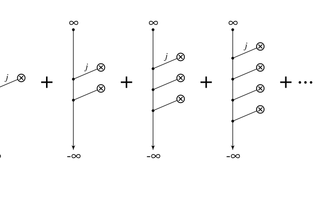
FIG. 1.: Diagrammatic representation of the series expansion for the light-cone gauge vector potential, Eq. (52). The circled crosses denote the positions at which the sources are being evaluated. The dots represent the ordered integrations coming from the gauge transformation into the light-cone gauge. A propagator connects each of these points to the sources.

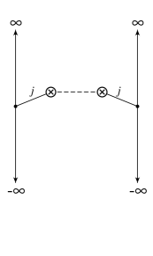
FIG. 2.: The lowest-order contribution to the gluon number density, Eq. (57). According to the power-counting rules described in the text, this diagram is proportional to $\alpha_{s}A$.

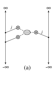
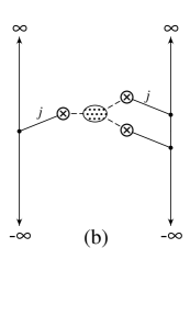
FIG. 3.: The contributions to the gluon number density (57) at 3rd order in $\rho$. According to the power-counting rules described in the text, both diagrams are proportional to $\alpha_{s}^{2}A$.

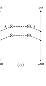
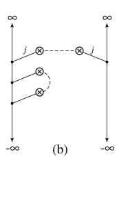
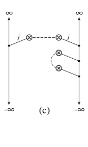
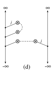
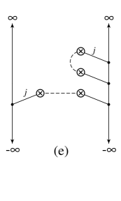
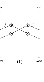
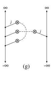
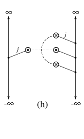
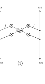
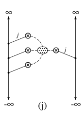
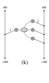
FIG. 4.: The contributions to the gluon number density (57) at 4th order in $\rho$. Diagrams (f)–(h) are non-planar, whereas diagrams (i)–(k) represent the (non-Gaussian) contribution from an irreducible 4-point charge density correlation function. According to the power-counting rules described in the text, diagrams (a)–(e) are proportional to $\alpha_{s}^{3}A^{4/3}$ whereas diagrams (f)–(h) are proportional to $\alpha_{s}^{3}A$.

TABLE I.: Mapping between the notations used in the discussion of the central limit theorem and those associated with the MV model.

	central limit theorem	MV model
	$\tau_{i}^{(p)}$	$\rho^{a}(x_{\scriptscriptstyle\parallel};\mathchoice{{\hbox{\boldmath$\displaystyle x$}}}{{\hbox{\boldmath$\textstyle x$}}}{{\hbox{\boldmath$\scriptstyle x$}}}{{\hbox{\boldmath$\scriptscriptstyle x$}}})$
	$(p)$	$x_{\scriptscriptstyle\parallel}$
	$i$	$\{a;\mathchoice{{\hbox{\boldmath$\displaystyle x$}}}{{\hbox{\boldmath$\textstyle x$}}}{{\hbox{\boldmath$\scriptstyle x$}}}{{\hbox{\boldmath$\scriptscriptstyle x$}}}\}$
	$N$	$A^{1/3}$
	$t_{i}\equiv{1\over N}\sum_{p=1}^{N}\tau_{i}^{(p)}$	$A^{-1/3}\rho_{2}^{a}(\mathchoice{{\hbox{\boldmath$\displaystyle x$}}}{{\hbox{\boldmath$\textstyle x$}}}{{\hbox{\boldmath$\scriptstyle x$}}}{{\hbox{\boldmath$\scriptscriptstyle x$}}})\equiv A^{-1/3}\int_{-\infty}^{\infty}dx_{\scriptscriptstyle\parallel}\thinspace\rho^{a}(x_{\scriptscriptstyle\parallel},\mathchoice{{\hbox{\boldmath$\displaystyle x$}}}{{\hbox{\boldmath$\textstyle x$}}}{{\hbox{\boldmath$\scriptstyle x$}}}{{\hbox{\boldmath$\scriptscriptstyle x$}}})$
	$W(\mathchoice{{\hbox{\boldmath$\displaystyle t$}}}{{\hbox{\boldmath$\textstyle t$}}}{{\hbox{\boldmath$\scriptstyle t$}}}{{\hbox{\boldmath$\scriptscriptstyle t$}}})$	$W[\rho_{2}(\mathchoice{{\hbox{\boldmath$\displaystyle x$}}}{{\hbox{\boldmath$\textstyle x$}}}{{\hbox{\boldmath$\scriptstyle x$}}}{{\hbox{\boldmath$\scriptscriptstyle x$}}})]$