Possible Supersymmetric Effects on Angular Distributions
in $B\to K^{*}(\to K\pi)\ell^{+}\ell^{-}$ Decays

Abstract

We investigate the angular distributions of the rare $B$ decay, $B\to K^{*}(\to K\pi)\ell^{+}\ell^{-}$, in general supersymmetric extensions of the standard model. We consider the new physics contributions from the operators $O_{7,8,9,10}$ in small invariant mass region of lepton pair. We show that the azimuthal angle distribution of the decay can tell us the new physics effects clearly from the behavior of the distribution, even if new physics does not change the decay rate substantially from the standard model prediction.

I Introduction

Rare decays of $B$ meson, $e.g.$ $b\to s\gamma$ and $b\to s\ell^{+}\ell^{-}$, are the most suitable candidates for study of new physics beyond the standard model (SM). Since their branching fractions are usually very small within the SM predictions, they can sometimes show up new physics with unexpectedly large values of decay rates. The decay $b\to s\gamma$, which has been already measured by the CLEO Collaboration [1], has shown that there is not much extra parameter space for its branching fraction from new physics [2]. The decay $b\to s\ell^{+}\ell^{-}$ suffers from severe backgrounds of $J/\psi$ and $\psi^{\prime}$ resonance contributions in the measurement of branching fraction, and so it may not be easy to uncover new physics cleanly [3]. However, a number of methods have been discussed to detect new physics through the details of the decay process, such as differential distributions or polarization effects [4, 5, 6].

Recently a new method utilizing the angular distribution of $B\to K^{*}(\to K\pi)\ell^{+}\ell^{-}$ has been proposed [7]. Imagine the decay configuration when $K^{*}$ is emitted to the direction of $+z$ and $\gamma^{*}$ is emitted to the opposite direction in the rest frame of $B$ meson. Here $\gamma^{*}$ is off-shell photon and it further decays into $\ell^{+}\ell^{-}$, and $K^{*}$ subsequently decays into $K\pi$. If we ignore small mixture of the longitudinal component, the angular momentum of $K^{*}$ is either $J_{z}=+1$ or $J_{z}=-1$, and the corresponding production amplitude is proportional to $C_{7R}$ or $C_{7L}$, respectively. Suppose the final $K$ meson is emitted to the direction of $(\theta_{K},~{}\phi)$ in the rest frame of $K^{*}$, where $\theta_{K}$ is a polar angle and $\phi$ is an azimuthal angle between the decay plane of ($K\pi$) and the decay plane of ($\ell^{+}\ell^{-}$). In the low invariant $m_{\ell^{+}\ell^{-}}$ region, electromagnetic operator terms are dominated and the decay amplitude for the whole process is proportional to

$$A~{}C_{7L}\exp(-i\phi)+B~{}C_{7R}\exp(+i\phi)+C~{},$$

where $A$, $B$ and $C$ are the real functions of the other angles.

In this new method, we can distinguish the new physics contribution from that of the SM even if the branching fraction of the decay is similar to the prediction of the SM: In the $B\to K^{*}\gamma$ decays the probability of $B$ meson decaying to left-handed (or right-handed) circular polarized $K^{*}$ is proportional to $|C_{7L}|^{2}$ (or $|C_{7R}|^{2}$), and therefore the polarization measurement of $K^{*}$ and $\gamma$ is useful for extracting the ratio of ${|C_{7L}|}/{|C_{7R}|}$. Even though the polarization of high energy real photon cannot be measured easily, we can still get some useful information through the azimuthal angle distribution in the low invariant mass region of dileptons for $B\to K^{*}(\to K\pi)\ell^{+}\ell^{-}$ decay. This is because the decay products of $K^{*}$ and the virtual photon $\gamma^{*}$ are responsible for this polarization measurements. In the SM, the operator $O_{7L}$ is dominant and the operator $O_{7R}$ is suppressed by ${\cal O}(m_{s}/m_{b})$. In this case, the angular distribution of the decay products is a flat function of the angle $\phi$ in the small lepton invariant mass region. If there is new physics contribution, the contribution of both operators can be equally important [7]. We can distinguish the new physics signal easily from the angular distribution of the decay $B\to K^{*}(\to K\pi)\ell^{+}\ell^{-}$, while the measured branching fraction for $B\to X_{s}\gamma$ can still be accommodated.

In this paper, we extend this method to calculate the angular distribution of $B\to K^{*}(K\pi)\ell^{+}\ell^{-}$ in generalized supersymmetry models (gSUSYs). In addition to the operator $O_{7R}$, we also consider the new operators $O_{9R}$ and $O_{10R}$. In the following section, we derive the general formula for the various angular distributions including the new operators. Section III is devoted to the numerical analysis and discussions in gSUSYs.

II Angular Distributions of the decay $B\to K^{*}(\to K+\pi)+\ell^{+}+\ell^{-}$

We start with the general effective Hamiltonian for the corresponding $b\to s\ell^{+}\ell^{-}$ decay [8],

$${\cal H}_{eff}(b\to s\ell^{+}\ell^{-}) = -\frac{G_{F}}{\sqrt{2}}V_{tb}V_{ts}^{*}{\alpha\over\pi}\sum_{i=7}^{10}(C_{iL}O_{iL}+C_{iR}O_{iR})~{}.$$ (1)

The operators $O_{i}$ relevant for us are

$$O_{7L} = \frac{em_{b}}{4\pi^{2}}(\bar{s}_{L}\sigma_{\mu\nu}b_{R})F^{\mu\nu},$$ (2)

$$O_{7R} = \frac{em_{b}}{4\pi^{2}}(\bar{s}_{R}\sigma_{\mu\nu}b_{L})F^{\mu\nu},$$ (3)

$$O_{8L} = {g_{s}\over 4\pi^{2}}~{}m_{b}\bar{s}_{L}\sigma^{\mu\nu}T^{a}b_{R}~{}G^{a}_{\mu\nu}$$ (4)

$$O_{8R} = {g_{s}\over 4\pi^{2}}~{}m_{b}\bar{s}_{R}\sigma^{\mu\nu}T^{a}b_{L}~{}G^{a}_{\mu\nu},$$ (5)

$$O_{9L} = ({\bar{s}}b)_{L}({\bar{\ell}}\ell)_{V},$$ (6)

$$O_{9R} = ({\bar{s}}b)_{R}({\bar{\ell}}\ell)_{V},$$ (7)

$$O_{10L} = ({\bar{s}}b)_{L}({\bar{\ell}}\ell)_{A},$$ (8)

$$O_{10R} = ({\bar{s}}b)_{R}({\bar{\ell}}\ell)_{A},$$ (9)

where in addition to the SM operators $O_{7L}$, $O_{8L}$, $O_{9L}$ and $O_{10L}$, we include new operators $O_{7R}$, $O_{8R}$, $O_{9R}$ and $O_{10R}$. The new physics effects can originate from any of the above operators. The operator $O_{7R}$ has already been introduced in Ref. [7], while the operators $O_{9R}$ and $O_{10R}$ are newly introduced in this paper. The operator $O_{8}$ is a chromo-magnetic dipole operator.

Relegating the details to Ref. [7], we introduce the helicity amplitudes for the decay

$$B\to K^{*}(\to K(p_{K})+\pi(p_{\pi}))+\ell^{+}(p_{+})+\ell^{-}(p_{-})~{},$$

which can be expressed by

$$H_{+1}^{L} = \left(a_{L}+c_{L}\sqrt{\lambda}\right)~{},$$ (10)

$$H_{-1}^{L} = \left(a_{L}-c_{L}\sqrt{\lambda}\right)~{},$$ (11)

$$H_{0}^{L} = -a_{L}\frac{P\cdot L}{pl}+\frac{b_{L}\lambda}{pl}~{},$$ (12)

$$H_{+1}^{R} = \left(a_{R}+c_{R}\sqrt{\lambda}\right)~{},$$ (13)

$$H_{-1}^{R} = \left(a_{R}-c_{R}\sqrt{\lambda}\right)~{},$$ (14)

$$H_{0}^{R} = -a_{R}\frac{P\cdot L}{pl}+\frac{b_{R}\lambda}{pl}~{},$$ (15)

with $P=p_{K}+p_{\pi}$, $L=p_{+}+p_{-}$, $p=\sqrt{P^{2}}$, $l=\sqrt{L^{2}}$, and $\lambda=(m_{B}^{2}-p^{2}-l^{2})^{2}/4-p^{2}l^{2}$. And $a_{R},~{}b_{R},~{}c_{R}$ and $a_{L},~{}b_{L},~{}c_{L}$ are given by

$$a_{L} = -C_{7-}\left[2(P\cdot L)g_{+}+L^{2}(g_{+}+g_{-})\right]+\frac{(C_{9-}-C_{10-})f}{2m_{b}}L^{2},$$ (16)

$$b_{L} = -2C_{7-}(g_{+}-L^{2}h)-\frac{(C_{9-}-C_{10-})a_{+}}{m_{b}}L^{2},$$ (17)

$$c_{L} = -2C_{7+}g_{+}+\frac{(C_{9+}-C_{10+})g}{m_{b}}L^{2},$$ (18)

$$a_{R} = -C_{7-}\left[2(P\cdot L)g_{+}+L^{2}(g_{+}+g_{-})\right]+\frac{(C_{9-}+C_{10-})f}{2m_{b}}L^{2},$$ (19)

$$b_{R} = -2C_{7-}(g_{+}-L^{2}h)-\frac{(C_{9-}+C_{10-})a_{+}}{m_{b}}L^{2},$$ (20)

$$c_{R} = -2C_{7+}g_{+}+\frac{(C_{9+}+C_{10+})g}{m_{b}}L^{2},$$ (21)

where the form factors $g$, $g_{+}$, $g_{-}$, $f$, $h$ and $a^{+}$ of $B\to K^{*}$ decay are defined in Refs. [7, 11, 12]. We introduced the Wilson coefficients $C_{7-,7+,9-,9+,10-,10+}$ as

$$C_{7-} = C_{7R}-C_{7L},~{}~{}~{}C_{7+}=C_{7R}+C_{7L},$$ (22)

$$C_{9-} = C_{9R}-C_{9L},~{}~{}~{}C_{9+}=C_{9R}+C_{9L},$$ (23)

$$C_{10-} = C_{10R}-C_{10L},~{}~{}~{}C_{10+}=C_{10R}+C_{10L}.$$ (24)

Using the above helicity amplitudes, the angular distribution of $B\to K^{*}(\to K\pi)\ell^{+}\ell^{-}$ is expressed by,

$$\frac{d^{5}\Gamma}{dp^{2}dl^{2}d\cos\theta_{K}d\cos\theta_{+}d\phi} = \frac{\alpha^{2}G_{F}^{2}g_{K^{*}K\pi}^{2}\sqrt{\lambda}p^{2}m_{b}^{2}|V_{tb}V_{ts}^{*}|^{2}}{64\times 8(2\pi)^{8}m_{B}^{3}l^{2}[(p^{2}-m_{K^{*}}^{2})^{2}+m_{K^{*}}^{2}\Gamma_{K^{*}}^{2}]}$$

$$\times \left\{4\cos^{2}\theta_{K}\sin^{2}\theta_{+}(|H_{0}^{R}|^{2}+|H_{0}^{L}|^{2})\right.$$ (33)

$$+\sin^{2}\theta_{K}(1+\cos^{2}\theta_{+})(|H_{+1}^{L}|^{2}+|H_{-1}^{L}|^{2}+|H_{+1}^{R}|^{2}+|H_{-1}^{R}|^{2})$$

$$-2\sin^{2}\theta_{K}\sin^{2}\theta_{+}\left[\cos 2\phi Re(H_{+1}^{R}H^{R*}_{-1}+H_{+1}^{L}H^{L*}_{-1})\right.$$

$$-\sin 2\phi\left.Im(H_{+1}^{R}H^{R*}_{-1}+H_{+1}^{L}H^{L*}_{-1})\right]$$

$$-\sin 2\theta_{K}\sin 2\theta_{+}\left[\cos\phi Re(H_{+1}^{R}H^{R*}_{0}+H_{-1}^{R}H_{0}^{R*}+H_{+1}^{L}H^{L*}_{0}+H_{-1}^{L}H_{0}^{L*})\right.$$

$$-\sin\phi\left.Im(H_{+1}^{R}H^{R*}_{0}-H_{-1}^{R}H_{0}^{R*}+H_{+1}^{L}H^{L*}_{0}-H_{-1}^{L}H_{0}^{L*})\right]$$

$$-2\sin^{2}\theta_{K}\cos\theta_{+}(|H_{+1}^{R}|^{2}-|H_{-1}^{R}|^{2}-|H_{+1}^{L}|^{2}+|H_{-1}^{L}|^{2})$$

$$+2\sin\theta_{+}\sin 2\theta_{K}\left[\cos\phi Re(H_{+1}^{R}H^{R*}_{0}-H_{-1}^{R}H_{0}^{R*}-H_{+1}^{L}H^{L*}_{0}+H_{-1}^{L}H_{0}^{L*})\right.$$

$$-\sin\phi\left.\left.Im(H_{+1}^{R}H^{R*}_{0}+H_{-1}^{R}H^{R*}_{0}-H_{+1}^{L}H^{L*}_{0}-H_{-1}^{L}H^{L*}_{0})\right]\right\}~{}.$$

Here we introduced the various angles as: $\theta_{K}$ is the polar angle of the $K$ meson momentum in the rest system of the $K^{*}$ meson with respect to the helicity axis, i.e. the outgoing direction of $K^{*}$. Similarly $\theta_{+}$ is the polar angle of the positron in the $\gamma^{*}$ rest system with respect to the helicity axis of the $\gamma^{*}$. And $\phi$ is the azimuthal angle between the planes of the two decays $K^{*}\to K\pi$ and $\gamma^{*}\to\ell^{+}\ell^{-}$.

If we integrate out the angles $\theta_{K}$ and $\theta_{+}$, we get the $\phi$ distribution

$$\frac{d\Gamma}{d\phi} = \int\frac{\alpha^{2}G_{F}^{2}g_{K^{*}K\pi}^{2}\sqrt{\lambda}p^{2}m_{b}^{2}|V_{tb}V_{ts}^{*}|^{2}}{9\times 16(2\pi)^{8}m_{B}^{3}l^{2}[(p^{2}-m_{K^{*}}^{2})^{2}+m_{K^{*}}^{2}\Gamma_{K^{*}}^{2}]}\left\{|H_{0}^{R}|^{2}+|H_{+1}^{R}|^{2}+|H_{-1}^{R}|^{2}\right.$$ (36)

$$|H_{0}^{L}|^{2}+|H_{+1}^{L}|^{2}+|H_{-1}^{L}|^{2}-\cos 2\phi Re(H^{R}_{+1}H^{R*}_{-1}+H_{+1}^{L}H^{L*}_{-1})$$

$$\left.+\sin 2\phi Im(H_{+1}^{R}H^{R*}_{-1}+H^{L}_{+1}H^{L*}_{-1})\right\}dp^{2}dl^{2}~{}.$$

Similarly, we can get the $\theta_{K}$ and $\theta_{+}$ angular distributions as following:

$$\frac{d\Gamma}{d\cos\theta_{K}} = \int\frac{(2\pi)\alpha^{2}G_{F}^{2}g_{K^{*}K\pi}^{2}\sqrt{\lambda}p^{2}m_{b}^{2}|V_{tb}V_{ts}^{*}|^{2}}{3\times 64(2\pi)^{8}m_{B}^{3}l^{2}[(p^{2}-m_{K^{*}}^{2})^{2}+m_{K^{*}}^{2}\Gamma_{K^{*}}^{2}]}\left\{2\cos^{2}\theta_{K}(|H_{0}^{R}|^{2}\right.$$ (38)

$$+\left.|H_{0}^{L}|^{2})+\sin^{2}\theta_{K}\left(|H_{+1}^{R}|^{2}+|H_{-1}^{R}|^{2}+|H_{+1}^{L}|^{2}+|H_{-1}^{L}|^{2}\right)\right\}dp^{2}dl^{2}~{},$$

and

$$\frac{d\Gamma}{d\cos\theta_{+}} = \int\frac{(2\pi)\alpha^{2}G_{F}^{2}g_{K^{*}K\pi}^{2}\sqrt{\lambda}p^{2}m_{b}^{2}|V_{tb}V_{ts}^{*}|^{2}}{6\times 64(2\pi)^{8}m_{B}^{3}l^{2}[(p^{2}-m_{K^{*}}^{2})^{2}+m_{K^{*}}^{2}\Gamma_{K^{*}}^{2}]}\left\{2\sin^{2}\theta_{+}(|H_{0}^{R}|^{2}+|H_{0}^{L}|^{2})\right.$$ (40)

$$+\left.(1+\cos\theta_{+})^{2}\left(|H_{+1}^{L}|^{2}+|H_{-1}^{R}|^{2}\right)+(1-\cos\theta_{+})^{2}\left(|H_{+1}^{R}|^{2}+|H_{-1}^{L}|^{2}\right)\right\}dp^{2}dl^{2}~{}.$$

Taking the narrow resonance limit of $K^{*}$ meson, i.e. using the equations

$$\Gamma_{K^{*}}=\frac{g_{K^{*}K\pi}^{2}m_{K^{*}}}{48\pi}~{},$$ (41)

$$\lim_{\Gamma_{K^{*}}\to 0}\frac{\Gamma_{K^{*}}m_{K^{*}}}{(p^{2}-m_{K^{*}}^{2})^{2}+m_{K^{*}}^{2}\Gamma_{K^{*}}^{2}}=\pi\delta(p^{2}-m_{K^{*}}^{2})~{},$$ (42)

we can perform the integration over $p^{2}$ and obtain the double differential branching fraction with respect to dilepton mass squared $l^{2}$ and angle variables,

$${dBr\over dl^{2}d\phi} = \tau_{B}{\alpha^{2}{G_{F}}^{2}\over 384\pi^{5}}\sqrt{\lambda}{{m_{b}}^{2}\over{m_{B}}^{3}l^{2}}|V_{ts}V_{tb}|^{2}{1\over 2\pi}\left\{|H_{0}^{R}|^{2}+|H_{+1}^{R}|^{2}+|H_{-1}^{R}|^{2}\right.$$ (45)

$$+|H_{0}^{L}|^{2}+|H_{+1}^{L}|^{2}+|H_{-1}^{L}|^{2}-\cos 2\phi Re(H^{R}_{+1}H^{R*}_{-1}+H_{+1}^{L}H^{L*}_{-1})$$

$$\left.+\sin 2\phi Im(H_{+1}^{R}H^{R*}_{-1}+H^{L}_{+1}H^{L*}_{-1})\right\}~{},$$

$${dBr\over dl^{2}d\cos\theta_{K}} = \tau_{B}{\alpha^{2}{G_{F}}^{2}\over 384\pi^{5}}\sqrt{\lambda}{{m_{b}}^{2}\over{m_{B}}^{3}l^{2}}|V_{ts}V_{tb}|^{2}{3\over 4}\left\{2\cos^{2}\theta_{K}(|H_{0}^{R}|^{2}+|H_{0}^{L}|^{2})\right.$$ (47)

$$\left.+\sin^{2}\theta_{K}(|H_{+1}^{R}|^{2}+|H_{-1}^{R}|^{2}+|H_{+1}^{L}|^{2}+|H_{-1}^{L}|^{2})\right\}~{},$$

$${dBr\over dl^{2}d\cos\theta_{+}} = \tau_{B}{\alpha^{2}{G_{F}}^{2}\over 384\pi^{5}}\sqrt{\lambda}{{m_{b}}^{2}\over{m_{B}}^{3}l^{2}}|V_{ts}V_{tb}|^{2}{3\over 8}\left\{2\sin^{2}\theta_{+}(|H_{0}^{R}|^{2}+|H_{0}^{L}|^{2})\right.$$ (49)

$$\left.+(1+\cos\theta_{+})^{2}(|H_{+1}^{L}|^{2}+|H_{-1}^{R}|^{2})+(1-\cos\theta_{+})^{2}(|H_{-1}^{L}|^{2}+|H_{+1}^{R}|^{2})\right\}~{},$$

and

$${dBr\over d{l^{2}}} = \tau_{B}{\alpha^{2}{G_{F}}^{2}\over 384\pi^{5}}\sqrt{\lambda}{{m_{b}}^{2}\over{m_{B}}^{3}l^{2}}|V_{ts}V_{tb}|^{2}\left\{|H_{0}^{R}|^{2}+|H_{+1}^{R}|^{2}+|H_{-1}^{R}|^{2}\right.$$ (51)

$$\left.+|H_{0}^{L}|^{2}+|H_{+1}^{L}|^{2}+|H_{-1}^{L}|^{2}\right\}~{},$$

where $\tau_{B}$ is the life time of $B$ meson, and we replace all $p$ by $m_{K^{*}}$ due to the $\delta$ function.

Finally, to eliminate the constant factors in Eq. (45), we define the normalized distribution,

$$r(\phi,\hat{s}) \equiv \left[{dBr\over d{l^{2}}d\phi}\right]/\left[{dBr\over d{l^{2}}}\right]$$ (52)

$$= {1\over 2\pi}\left\{1-\frac{\cos 2\phi Re(H^{R}_{+1}H^{R*}_{-1}+H_{+1}^{L}H^{L*}_{-1})-\sin 2\phi Im(H_{+1}^{R}H^{R*}_{-1}+H^{L}_{+1}H^{L*}_{-1})}{|H_{0}^{R}|^{2}+|H_{+1}^{R}|^{2}+|H_{-1}^{R}|^{2}+|H_{0}^{L}|^{2}+|H_{+1}^{L}|^{2}+|H_{-1}^{L}|^{2}}\right\},$$ (53)

where $\hat{s}=l^{2}/m_{B}^{2}$. The distribution $r(\phi,\hat{s})$ is the probability for finding $K$ meson per unit radian region in the direction of azimuthal angle $\phi$. Therefore, the normalized distribution $r(\phi,\hat{s})$ oscillates around its average value given by ${1\over 2\pi}\simeq 0.16$.

III Gluino Mediated Flavor Changing Neutral Current and its Numerical Analyses

In this section we consider the flavor changing neutral current (FCNC) in generalized supersymmetric models (gSUSYs). In gSUSYs, the soft mass terms for sfermions can lead to potentially large FCNC [9]. In the mass-insertion-approximation (MIA) [10], one chooses a basis for fermion and sfermion states, in which all the couplings of these particles to neutral gauginos are flavor diagonal. Flavor changes in the squark sector are provided by the non-diagonality of the sfermion propagators, which can be expressed in terms of the dimensionless parameters $(\delta_{ij}^{q})_{MN}$,

$$(\delta_{ij}^{q})_{MN}=\frac{(m_{ij}^{\tilde{q}})^{2}_{MN}}{\tilde{m}}~{}~{}~{}~{}(M,N=L,R)~{},$$ (54)

where $(m_{ij}^{\tilde{q}})^{2}_{MN}$ are the off-diagonal elements of the $\tilde{q}$ mass squared matrix that mixes flavor $i,j$ for both left- and right-handed scalars, and $\tilde{m}$ is the average squark mass. The expressions for the Wilson coefficients at $M_{W}$ scale due to the FCNC gluino exchange diagrams [9] are

$$C_{7L}^{\rm SUSY}(M_{W}) = {8\pi\alpha_{s}\over 9\sqrt{2}G_{F}\tilde{m}^{2}\lambda_{t}}~{}\left[\left(\delta_{23}^{d}\right)_{LL}M_{3}(x)+\left(\delta_{23}^{d}\right)_{LR}{m_{\tilde{g}}\over m_{b}}M_{1}(x)\right]~{},$$ (55)

$$C_{8L}^{\rm SUSY}(M_{W}) = {\pi\alpha_{s}\over\sqrt{2}G_{F}\tilde{m}^{2}\lambda_{t}}~{}\left[\left(\delta_{23}^{d}\right)_{LL}\left({1\over 3}M_{3}(x)+3M_{4}(x)\right)+\left(\delta_{23}^{d}\right)_{LR}{m_{\tilde{g}}\over m_{b}}\left({1\over 3}M_{1}(x)+3M_{2}(x)\right)\right],$$ (56)

$$C_{9L}^{\rm SUSY}(M_{W}) = {16\pi\alpha_{s}\over 9\sqrt{2}G_{F}\tilde{m}^{2}\lambda_{t}}~{}\left(\delta_{23}^{d}\right)_{LL}P_{1}(x)~{},$$ (57)

and

$$C_{7R}^{\rm SUSY}(M_{W}) = {8\pi\alpha_{s}\over 9\sqrt{2}G_{F}\tilde{m}^{2}\lambda_{t}}~{}\left[\left(\delta_{23}^{d}\right)_{RR}M_{3}(x)+\left(\delta_{23}^{d}\right)_{RL}{m_{\tilde{g}}\over m_{b}}M_{1}(x)\right]~{},$$ (58)

$$C_{8R}^{\rm SUSY}(M_{W}) = {\pi\alpha_{s}\over\sqrt{2}G_{F}\tilde{m}^{2}\lambda_{t}}~{}\left[\left(\delta_{23}^{d}\right)_{RR}\left({1\over 3}M_{3}(x)+3M_{4}(x)\right)+\left(\delta_{23}^{d}\right)_{RL}{m_{\tilde{g}}\over m_{b}}\left({1\over 3}M_{1}(x)+3M_{2}(x)\right)\right],$$ (59)

$$C_{9R}^{\rm SUSY}(M_{W}) = {16\pi\alpha_{s}\over 9\sqrt{2}G_{F}\tilde{m}^{2}\lambda_{t}}~{}\left(\delta_{23}^{d}\right)_{RR}P_{1}(x)~{},$$ (60)

with $\lambda_{t}\equiv V_{ts}^{*}V_{tb}$. The functions $M_{1,3}(x)$ and $P_{1}(x)$ are defined as

$$M_{1}(x) = {1+4x-5x^{2}+(4x+2x^{2})\ln x\over 2(1-x)^{4}}~{},$$ (61)

$$M_{2}(x) = -x^{2}{5-4x-x^{2}+(2+4x)\ln x\over 2(1-x)^{4}}~{},$$ (62)

$$M_{3}(x) = {-1+9x+9x^{2}-17x^{3}+(18x^{2}+6x^{3})\ln x\over 12(x-1)^{5}}~{},$$ (63)

$$M_{4}(x) = {-1-9x+9x^{2}+x^{3}-6(x+x^{2})\ln x\over 6(x-1)^{5}}~{},$$ (64)

$$P_{1}(x) = {1-6x+18x^{2}-10x^{3}-3x^{4}+12x^{3}\ln x\over 18(x-1)^{5}}~{},$$ (65)

where $x\equiv m^{2}_{\tilde{g}}/{\tilde{m}}^{2}$ and $m_{\tilde{g}}$ is gluino mass.

In addition to the above gSUSYs contributions, the usual SM contributions $C_{7L}^{\rm SM}$, $C_{8L}^{\rm SM}$, $C_{9L}^{\rm SM}$, and $C_{10L}^{\rm SM}$ are already known for years, which we will not show here. Please look at Refs. [7, 8] for details of the SM contributions. Including the QCD corrections, we get the Wilson coefficients at $m_{b}$ scale as

$$C_{7L}(m_{b}) = -0.31+0.67C_{7L}^{\rm SUSY}(M_{W})+0.09C_{8L}^{\rm SUSY}(M_{W})~{},$$ (66)

$$C_{7R}(m_{b}) = 0.67C_{7R}^{\rm SUSY}(M_{W})+0.09C_{8R}^{\rm SUSY}(M_{W})~{},$$ (67)

$$C_{9L}(m_{b}) = C_{9L}^{\rm SM}(m_{b})+C_{9L}^{\rm SUSY}(M_{W})~{},$$ (68)

$$C_{9R}(m_{b}) = C_{9R}^{\rm SUSY}(M_{W})~{}.$$ (69)

Here, $-0.31$ in Eq. (66) is the SM value of $C_{7L}(m_{b})$. New physics contributions $C_{iL}^{\rm SUSY}(M_{W})$, $C_{iR}^{\rm SUSY}(M_{W})$ come from Eqs. (57,60). For $C_{10}$, there is no new physics contribution,

$$C_{10L}(m_{b}) = C_{10L}^{\rm SM}(m_{b})~{},$$ (70)

$$C_{10R}(m_{b}) = 0~{}.$$ (71)

Then we can get the complete formula for angular distributions of $B\to K^{*}\ell^{+}\ell^{-}$, Eq. (53).

The operators $O_{7L}$ and $O_{7R}$ contribute to the rare radiative decay $b\to s\gamma$. Their Wilson coefficients have been constrained by the experimental measurements of the decay. The decay width for inclusive $b\to s\gamma$ decay is given in terms of the operators $O_{7L}$ and $O_{7R}$. It is convenient to normalize this radiative partial width to the semileptonic decay $b\to ce\bar{\nu}$ in terms of the ratio $R$,

$$R\equiv{\Gamma(b\to s\gamma)\over\Gamma(b\to ce\bar{\nu})}={6\over\pi}{|V_{ts}^{*}V_{tb}|^{2}\over|V_{cb}|^{2}}{\alpha_{em}\over f({m_{c}/m_{b}})}{|C_{7L}(m_{b})|^{2}+|C_{7R}(m_{b})|^{2}\over 1-{2\over 3\pi}\alpha_{s}(m_{b})g({m_{c}/m_{b}})},$$ (72)

where the functions $f(x)$ and $g(x)$ are phase space and QCD correction factors [13], respectively. The $b\to s\gamma$ branching fraction is obtained by

$${\cal BR}(b\to s\gamma)\simeq{\cal BR}(B\to X_{c}l\nu)_{\rm exp.}\times R\simeq(0.105)\times R.$$ (73)

For ${\cal BR}(b\to s\gamma)$, we use the present experimental value [1] of the branching fraction for the inclusive $B\to X_{s}\gamma$ decay,

$${\cal BR}(B\to X_{s}\gamma)=(3.15\pm 0.35\pm 0.32\pm 0.26)\times 10^{-4}.$$ (74)

Constrained by this experiment, we derive from Eq. (72)

$$|C_{7L}(m_{b})|^{2}+|C_{7R}(m_{b})|^{2}=0.081\pm 0.014.$$ (75)

In the numerical calculations, we use the form factors calculated in Ref. [11]. They are listed in Table  I for zero momentum transfer. The evolution formula for these form factors is

$$f_{i}(l^{2})=\frac{f_{i}(0)}{1-\sigma_{1}l^{2}+\sigma_{2}l^{4}}~{},$$ (76)

where $l^{2}=(p_{\ell^{+}}+p_{\ell^{-}})^{2}$. The corresponding values $\sigma_{1}$ and $\sigma_{2}$ for each form factors are also listed in Table 1.

The decay $B\to K^{*}+J/\psi(\to\ell^{+}\ell^{-})$ is a possible background for our $B\to K^{*}\ell^{+}\ell^{-}$ decay at the $J/\psi$ resonance region, so as the $\psi^{\prime}$, $etc$. Therefore, only the low invariant mass region of the lepton pair is good for clean measurements. The helicity amplitudes are dominated by the two coefficients $C_{7L}$ and $C_{7R}$ in the region of low invariant mass, as given by

$$H^{L,R}_{+1} \simeq -4g_{+}C_{7R}\sqrt{\lambda}~{},$$ (77)

$$H^{L,R}_{-1} \simeq 4g_{+}C_{7L}\sqrt{\lambda}~{},$$ (78)

$$H^{L,R}_{0} \simeq 0~{}.$$ (79)

In the small invariant mass limit $\hat{s}\ll 1$, $r(\phi,\hat{s})$, defined in Eq. (53), is approximately written as,

$$r(\phi,~{}\hat{s}\ll 1) \simeq {1\over 2\pi}\left\{1+\cos 2\phi\frac{Re(C_{7R}C_{7L}^{*})}{|C_{7R}|^{2}+|C_{7L}|^{2}}-\sin 2\phi\frac{Im(C_{7R}C_{7L}^{*})}{|C_{7R}|^{2}+|C_{7L}|^{2}}\right\}.$$ (80)

In the SM case, $C_{7R}\simeq 0$ and therefore the above approximate formula is reduced to

$$r(\phi,~{}\hat{s}\to 0)_{\rm SM} \simeq {1\over 2\pi}.$$ (81)

In Fig. 1 we can see that it is almost a constant distribution of $\phi$ in the small $\hat{s}$ region. As $\hat{s}$ increases, the contributions from the operator $O_{9}$ and $O_{10}$ makes $(\sim-\cos 2\phi)$ behavior. However, the new physics contributions can give quite different distributions depending on the model, and we can probe new physics efficiently. Here we discuss the gSUSYs contribution to the distribution $r(\phi,\hat{s})$. For simplicity, we assume that $|\delta_{LR}|=|\delta_{RL}|$ and $|\delta_{LL}|=|\delta_{RR}|$, and consider two cases: LR mixing dominating case and LL mixing dominating case.

First we consider the LR mixing dominating situation, $i.e.$ $|\delta_{LL}|\sim|\delta_{RR}|\ll|\delta_{LR}|\sim|\delta_{RL}|$. Fig. 2 shows the distribution $r(\phi,\hat{s})$ for $\delta_{LR}=\delta_{RL}=|\lambda_{t}|$ case with $x=0.3$, $\tilde{m}=960$ GeV. This corresponds to $C_{7L}=0.017$ and $C_{7R}=0.333$. Since $C_{7L}\ll C_{7R}$ and both are real, the approximate formula (80) becomes

$$r(\phi,~{}\hat{s}\ll 1)\simeq{1\over 2\pi}\left\{1+\cos 2\phi\left|\frac{C_{7L}}{C_{7R}}\right|\right\}.$$ (82)

This $(\sim\cos 2\phi)$ behavior is shown in Fig. 2. On the other hand, Fig. 3 shows the distribution $r(\phi,\hat{s})$ for $\delta_{LR}=-\delta_{RL}=|\lambda_{t}|$ case with $x=0.3$, $\tilde{m}=960$ GeV. This corresponds to $C_{7L}=0.017$ and $C_{7R}=-0.333$. In this case the approximate formula (80) becomes

$$r(\phi,~{}\hat{s}\ll 1)\simeq{1\over 2\pi}\left\{1-\cos 2\phi\left|\frac{C_{7L}}{C_{7R}}\right|\right\}.$$ (83)

This $(\sim-\cos 2\phi)$ behavior is shown in Fig. 3 explicitly for the small $\hat{s}$ region. In Figs. 2 and  3, we used the same values of $x$ and $\tilde{m}$: The branching fractionss of both $b\to s\gamma$ and $b\to s\ell^{+}\ell^{-}$ are unchanged for the two situations, and we cannot separate these two situations by using only branching fraction measurements. However, we can see that the angular distributions, shown in Figs. 2 and 3, can easily distinguish the relative sign of $\delta_{LR}$ and $\delta_{RL}$.

For the LL mixing dominating case, $i.e.$ $|\delta_{LR}|\sim|\delta_{RL}|\ll|\delta_{LL}|\sim|\delta_{RR}|$, we also show two cases. First we choose $\delta_{LL}=\delta_{RR}=e^{i\frac{\pi}{4}}$, with $x=0.8$, $\tilde{m}=250$ GeV. This corresponds to $C_{7L}=-0.16+i~{}0.15$ and $C_{7R}=+0.15+i~{}0.15$, $i.e.$ ${C_{7R}}/{C_{7L}}\sim e^{i\frac{3\pi}{2}}$ case. Using this set of parameters, the formula (80) becomes

$$r(\phi,~{}\hat{s}\ll 1) \simeq {1\over 2\pi}\left\{1+\frac{1}{2}\sin 2\phi\right\}.$$ (84)

Fig. 4 shows this $(\sim\sin 2\phi)$ behavior clearly. On the other hand, Fig. 5 shows the distribution $r(\phi,\hat{s})$ for $\delta_{LL}=-\delta_{RR}=e^{i\frac{\pi}{4}}$ case with $x=0.8$, $\tilde{m}=250$ GeV. This corresponds to $C_{7L}=-0.16+i~{}0.15$ and $C_{7R}=-0.15-i~{}0.15$, i.e, ${C_{7R}}/{C_{7L}}\sim e^{i\frac{\pi}{2}}$ case. The approximate formula becomes

$$r(\phi,~{}\hat{s}\ll 1) \simeq {1\over 2\pi}\left\{1-\frac{1}{2}\sin 2\phi\right\}.$$ (85)

The $(\sim-\sin 2\phi)$ behavior is shown in Fig. 5. From Figs. 4 and 5, we can see that the angular distribution can distinguish the relative phase between $\delta_{LL}$ and $\delta_{RR}$ easily, even if we use the same values of parameters, $x$ and $\tilde{m}$.

The polar angle distribution functions in Eqs. (47,49) depend only on the modular square terms of the helicity amplitudes, which give the decay width of the semileptonic decay. If the branching fraction is fixed by experiments, these two angle distributions cannot distinguish new physics contribution from the SM. On the other hand, they can serve as a double check of whether the branching fraction is different from the SM predictions.

In conclusion, we have calculated the angular distribution of the rare decay, $B\to K^{*}+(\to K\pi)+\ell^{+}+\ell^{-}$, in general supersymmetric extensions of the standard model. The azimuthal angle ($\phi$) distribution in gSUSYs can be quite different from that of the SM, while the measured branching fraction for $B\to X_{s}\gamma$ can be accommodated within the standard model prediction. In the standard model it is found to be almost a constant under the variation of the angle $\phi$ in small invariant mass region, while in gSUSYs the distribution can show $(\sim\pm\cos 2\phi)$ or $(\pm\sin 2\phi)$ behavior depending on the gSUSYs parameters. We showed that the angular distribution of the decay can tell us the new physics effects clearly from the behavior of the distribution, even if new physics does not change the decay rate substantially: We would be able to tell the relative phase between the mixing parameters $\delta_{LR}$ and $\delta_{RL}$ (or $\delta_{LL}$ and $\delta_{RR}$), even though the decay rate of gSUSYs were exactly the same as that of the SM.

TABLE I.: Form factors in zero momentum transfer and parameters of evolution formula [11].

	$g$	$f$	$a_{+}$	$a_{-}$	$g_{+}$	$g_{-}$	$h$
$f_{i}(0)$	0.063	2.01	-0.0454	0.053	-0.3540	0.313	-0.0028
$\sigma_{1}$	0.0523	0.0212	0.039	0.044	0.0523	0.053	0.0657
$\sigma_{2}$	0.00066	0.00009	0.00004	0.00023	0.0007	0.00067	0.0010

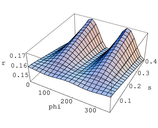
FIG. 1.: The distribution $r(\phi,\hat{s})$ for the SM case, where $C_{7R}\simeq 0$.

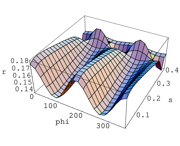
FIG. 2.: The distribution $r(\phi,\hat{s})$ for $\delta_{LR}=\delta_{RL}=|\lambda_{t}|$ case, with $x=0.3$, $\tilde{m}=960$ GeV. This corresponds to $C_{7L}=0.017$, $C_{7R}=0.333$.

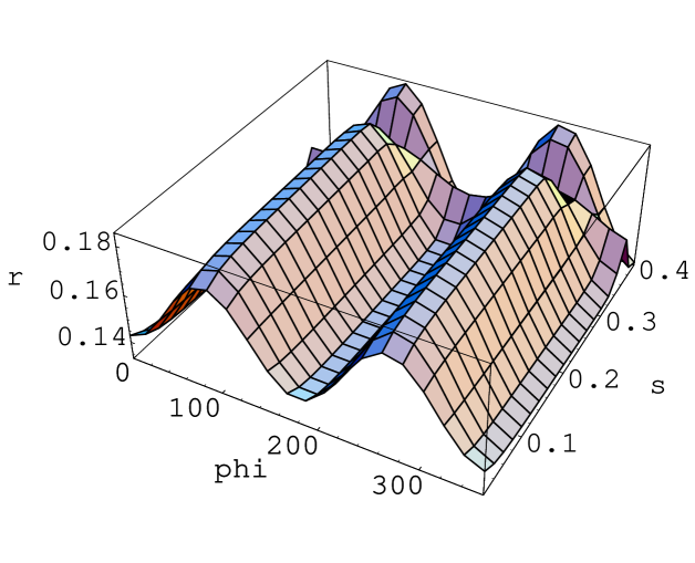
FIG. 3.: The distribution $r(\phi,\hat{s})$ for $\delta_{LR}=-\delta_{RL}=|\lambda_{t}|$ case, with $x=0.3$, $\tilde{m}=960$ GeV. This corresponds to $C_{7L}=0.017$, $C_{7R}=-0.333$.

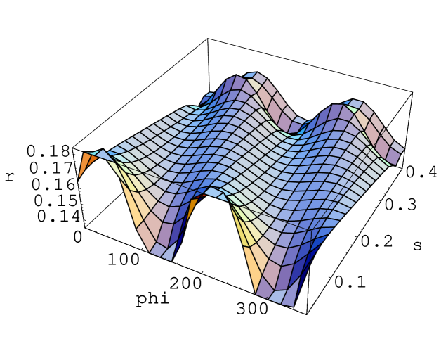
FIG. 4.: The distribution $r(\phi,\hat{s})$ for $\delta_{LL}=\delta_{RR}=e^{i\frac{\pi}{4}}$ case, with $x=0.8$, $\tilde{m}=250$ GeV. In this case, $C_{7R}/C_{7L}\simeq e^{i\frac{3}{2}\pi}$.

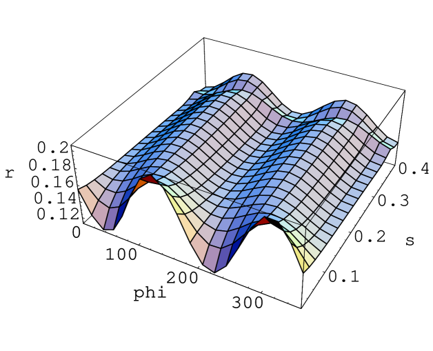
FIG. 5.: The distribution $r(\phi,\hat{s})$ for $\delta_{LL}=-\delta_{RR}=e^{i\frac{\pi}{4}}$ case, with $x=0.8$, $\tilde{m}=250$ GeV. In this case, $C_{7R}/C_{7L}\simeq e^{i\frac{\pi}{2}}$.