IFT-UAM/CSIC 01-03, FTUAM 01/02, KA-TP-3-2001 hep-ph/0102169

Decoupling Properties of MSSM particles
in Higgs and Top Decays

H. E. Haber^a, M. J. Herrero^b, H. E. Logan^c,
S. Peñaranda^d, S. Rigolin^e and D. Temes^b

^a Santa Cruz Institute for Particle Physics, University of California.
^b Departamento de Física Teórica, Universidad Autónoma de Madrid.
^c Theoretical Physics Department, Fermi National Accelerator Laboratory.
^d Institut für Theoretische Physik, Universität Karlsruhe.
^e Department of Physics, University of Michigan.

We study the supersymmetric (SUSY) QCD radiative corrections, at the one-loop level, to $h^{0}$, $H^{\pm}$ and $t$ quark decays, in the context of the Minimal Supersymmetric Standard Model (MSSM) and in the decoupling limit. The decoupling behaviour of the various MSSM sectors is analyzed in some special cases, where some or all of the SUSY mass parameters become large as compared to the electroweak scale. We show that in the decoupling limit of both large SUSY mass parameters and large CP-odd Higgs mass, the $\Gamma(h^{0}\rightarrow b\overline{b})$ decay width approaches its Standard Model value at one loop, with the onset of decoupling being delayed for large $\tan\beta$ values. However, this decoupling does not occur if just the SUSY mass parameters are taken large. A similar interesting non-decoupling behaviour, also enhanced by $\tan\beta$, is found in the SUSY-QCD corrections to the $\Gamma(H^{+}\rightarrow t\overline{b})$ decay width at one loop. In contrast, the SUSY-QCD corrections in the $\Gamma(t\rightarrow W^{+}b)$ decay width do decouple and this decoupling is fast.

Presented at the

5th International Symposium on Radiative Corrections
(RADCOR–2000)
Carmel CA, USA, 11–15 September, 2000

1 Introduction

The study of radiative corrections to Standard Model (SM) couplings may provide crucial clues in exploring new physics beyond the reach of present accelerators. In particular, suppose that a light Higgs boson, $h^{0}$, were discovered in the mass range predicted by the minimal supersymmetric extension of the Standard Model (MSSM), but supersymmetric (SUSY) particles were not found. Then, a precise measurement of Higgs couplings to SM particles, which are sensitive to radiative corrections, could provide indirect information about the existence of SUSY in Nature and some indication of the preferred region of the SUSY parameter space. For example, one could predict (in the context of the MSSM) whether the data favored a SUSY spectrum below the 1 TeV energy scale. Similar studies can be performed by considering alternative observables as, for instance, the partial widths of top and Higgs decays into SM particles, and by comparing their predictions in the MSSM and the SM.

In this comparison of the MSSM and SM predictions for observables involving SM particles in the external legs, it is interesting to consider some particular limiting situations. The first one is when the genuine SUSY spectrum is very heavy as compared to the electroweak scale, $M_{SUSY}\gg M_{Z}$, where $M_{SUSY}$ represents generically the masses of the SUSY particles. This situation corresponds to the decoupling of SUSY particles from the rest of the MSSM spectrum, namely, the SM particles and the MSSM Higgs sector containing $h^{0}$, $H^{0}$, $A^{0}$ and $H^{\pm}$. The second one is when the extra Higgs bosons, $H^{0}$, $A^{0}$ and $H^{\pm}$ are very heavy, but $h^{0}$ and the genuine SUSY particles are closer to the electroweak scale. This decoupling limit can be reached by considering $M_{A}\gg M_{Z}$, where $M_{A}$ is the mass of the CP-odd neutral Higgs boson of the MSSM. In addition, there is the limiting situation where both $M_{SUSY}$ and $M_{A}$ are large, and the decoupling of all non-standard particles from the SM physics is expected. This decoupling is known to occur in tree-level physics and in some one-loop physics. In particular, the tree-level couplings of $h^{0}$ to fermion pairs and gauge bosons tend to their SM values if $M_{A}\gg M_{Z}$ [1]. As a consequence of this decoupling, distinguishing the lightest MSSM Higgs boson in the large $M_{A}$ limit from the Higgs boson of the SM will be very difficult.

Formally, the decoupling of all non-standard MSSM particles implies that in the effective low-energy theory, all observables involving SM particles in the external legs tend to their SM values in the limit of large SUSY masses and large $M_{A}$. It has been shown that all the genuine SUSY particles in the MSSM and the heavy Higgs bosons $H^{0}$, $A^{0}$ and $H^{\pm}$, decouple at one-loop order from the low-energy electroweak gauge boson physics [2]. In particular, the contributions of the SUSY particles to low-energy processes either fall as inverse powers of the SUSY mass parameters or can be absorbed into counterterms for the tree-level couplings of the low-energy theory and, therefore, they decouple in the same spirit as established in the Appelquist-Carazzone Theorem [3]. As a result, the radiative corrections involving SUSY particles go to zero in the asymptotic large SUSY mass limit.

Our purpose here is to determine the decoupling behaviour in the previous limiting situations of several observables, including radiative corrections at one-loop, with the hope that for some of them either the decoupling does not occur totally or, in case it occurs, it proceeds slowly such that there may remain significant signals of new physics beyond SM, even for a heavy SUSY spectra.

In this paper we focus on the partial widths of $h^{0}\rightarrow b\overline{b}$, $H^{+}\rightarrow t\overline{b}$ and $t\rightarrow W^{+}b$ decays, with special emphasis on the first one, whose corresponding branching ratio will be crucial for the experimental Higgs boson searches at the upcoming Tevatron Run 2 [4, 5]. We study the MSSM radiative corrections to these observables at the one-loop level and to leading order in $\alpha_{s}$, and we analyze in detail their behavior in the previously mentioned decoupling limits. These corrections are due to the SUSY-QCD (SQCD) sector and arise from gluinos and third generation-squark exchange. Because of the dependence on the strong coupling constant, these are expected to be the most significant one-loop MSSM contributions over much of the MSSM parameter space. We will show that in the limit of large $M_{A}$ (in this limit one also has $M_{H^{0}},M_{H^{\pm}}\gg M_{Z}$) and large sbottom and gluino masses ($M_{\tilde{b}_{i}},M_{\tilde{g}}\gg M_{Z}$), the SM expression for the $h^{0}\rightarrow b\overline{b}$ one-loop partial width is recovered [6]. That is, the SQCD corrections to the $\Gamma(h^{0}\rightarrow b\overline{b})$ partial width decouple in the limit of large SUSY masses and large $M_{A}$. In particular, we examine the case of large $\tan\beta$, for which the SQCD corrections are enhanced. This enhancement can delay the onset of decoupling and give rise to a significant one-loop correction, even for moderate to large values of the SUSY masses. This decoupling, however, does not occur, if either $M_{SUSY}$ (characterizing a common mass scale for gluino and sbottom masses) or $M_{A}$ are kept fixed while the other is taken large. A similar non-decoupling phenomenon of the SQCD corrections to one-loop when $M_{A}$ is fixed and the sbottom, stop and gluinos masses are considered large is found in the $H^{+}\rightarrow t\overline{b}$ decay [7]. The SQCD corrections to one-loop in the $t\rightarrow W^{+}b$ decay, however, do decouple and this decoupling proceeds fast. We present here just a summary of the main results and refer the reader to refs. [6, 7] for more details.

2 Decoupling limit in the Higgs sector

The decoupling limit in the Higgs sector of the MSSM was first studied in ref. [1]. In short, it is defined by considering the CP-odd Higgs mass much larger than the electroweak scale, $M_{A}\gg M_{Z}$, and leads to a particular spectrum in the Higgs sector with very heavy $H^{0}$, $H^{\pm}$ and $A^{0}$ bosons, and a light $h^{0}$ boson. For a review of the MSSM Higgs sector, see ref. [8].

At tree level, if $M_{A}\gg M_{Z}$, the Higgs masses are,

$M_{H^{o}}\simeq M_{H^{\pm}}\simeq M_{A}\gg M_{Z}\,\,\,,\,\,M_{h^{o}}\simeq M_{Z}|cos2\beta|\,.$
That is, at tree-level there exists a CP-even Higgs, $h^{0}$, lighter than the $Z$ boson.

Concerning the neutral Higgs couplings, their tree-level values in the MSSM normalized to SM couplings and for arbitrary $M_{A}$, are given in table 1.

$\phi$		$g_{\phi\overline{t}t}$	$g_{\phi\overline{b}b}$	$g_{\phi VV}$
SM	$H$	1	1	1
MSSM	$h^{o}$	${\cos\alpha/\sin\beta}$	${-\sin\alpha/\cos\beta}$	${\sin(\beta-\alpha)}$
	$H^{o}$	$\sin\alpha/\sin\beta$	$\cos\alpha/\cos\beta$	$\cos(\beta-\alpha)$
	$A^{o}$	$1/\tan\beta$	$\tan\beta$	0

Table 1: Higgs couplings in the MSSM normalized to SM couplings

Notice that by expanding in inverse powers of $M_{A}$, we get:

${\frac{\cos\alpha}{\sin\beta}}\simeq 1+\cal{O}$$(M_{Z}^{2}/M_{A}^{2})$$\,,\,$ ${-\frac{\sin\alpha}{\cos\beta}}\simeq 1+\cal{O}$$(M_{Z}^{2}/M_{A}^{2})$

${\sin(\beta-\alpha)}\simeq 1+\cal{O}$$(M_{Z}^{4}/M_{A}^{4})$.

Therefore, the $h^{0}$ tree-level couplings in the decoupling limit, $M_{A}\gg M_{Z}$, tend to their SM values, as expected.

Beyond tree level, it has been shown [9] that, in this same decoupling limit, the Higgs masses keep a similar pattern as at tree level, that is, very heavy $H^{0}$, $H^{\pm}$ and $A^{0}$ bosons, and a light $h^{0}$ boson. The particular values of their masses depend of course on the MSSM parameters, but for $M_{A}\gg M_{Z}$,

$M_{H^{o}}\simeq M_{H^{\pm}}\simeq M_{A}\gg M_{Z}\,,$

$M_{h^{o}}\leq 130-135\,GeV\,.$

In this work we will go beyond tree level and study the decoupling behaviour of heavy SUSY particles and heavy Higgses, at one-loop level, in Higgs bosons and top quark decays.

3 Decoupling limit in the SUSY-QCD sector

The sbottom and stop mass matrices, in the MSSM, are given respectively by:

$${\hat{M}}_{\tilde{b}}^{2}=\left(\begin{array}[]{cc}{{M_{{\scriptscriptstyle{\tilde{Q}}}}^{2}}+m_{b}^{2}-M_{Z}^{2}(\frac{1}{2}+Q_{b}s_{{\scriptscriptstyle W}}^{2})\cos{2\beta}}&{m_{\scriptscriptstyle b}({A_{b}}-{\mu}\tan{\beta})}\\ {m_{\scriptscriptstyle b}({A_{b}}-{\mu}\tan{\beta})}&{{M_{{\scriptscriptstyle{\tilde{D}}}}^{2}}+m_{b}^{2}+M_{Z}^{2}Q_{b}s_{{\scriptscriptstyle W}}^{2}\cos{2\beta}}\end{array}\right)$$

and

$${\hat{M}}_{\tilde{t}}^{2}=\left(\begin{array}[]{cc}{{M_{{\scriptscriptstyle{\tilde{Q}}}}^{2}}+m_{t}^{2}+M_{Z}^{2}(\frac{1}{2}-Q_{t}s_{{\scriptscriptstyle W}}^{2})\cos{2\beta}}&{m_{\scriptscriptstyle t}({A_{t}}-{\mu}\cot{\beta})}\\ {m_{\scriptscriptstyle t}({A_{t}}-{\mu}\cot{\beta})}&{{M_{{\scriptscriptstyle{\tilde{U}}}}^{2}}+m_{t}^{2}+M_{Z}^{2}Q_{t}s_{{\scriptscriptstyle W}}^{2}\cos{2\beta}}\end{array}\right)$$

In order to get heavy squarks and heavy gluinos, we need to choose properly the soft SUSY breaking parameters and the $\mu$-parameter. Since here we are interested in the limiting situation where the whole SUSY spectrum is heavier than the electroweak scale, we have made the following assumptions for the soft breaking squark mass parameters, trilinear terms, $\mu$-parameter and gluino mass (see ref. [6] for more details),

$$M_{SUSY}\sim M_{{\scriptscriptstyle{\tilde{Q}}}}\sim M_{{\scriptscriptstyle{\tilde{D}}}}\sim M_{{\scriptscriptstyle{\tilde{U}}}}\sim M_{\tilde{g}}\sim\mu\sim A_{b}\sim A_{t}\gg M_{Z},$$

where $M_{SUSY}$ represents generically a common SUSY large mass scale.

Besides, we have considered two extreme cases, maximal and minimal mixing, which, for the large mass limit we are studing, imply certain constraints on the squark mass differences. Thus, given the generic mass matrix,

$${\hat{M}}^{2}_{\tilde{q}}\equiv\left(\begin{array}[]{cc}{M_{L}^{2}}&{m_{q}X_{q}}\\ {m_{q}X_{q}}&{M_{R}^{2}}\end{array}\right),$$

the two limiting cases are reached by choosing the relative size of $M_{L,R}$ and $X_{q}$ as follows,

A.-Close to maximal mixing: $\theta_{\tilde{q}}\sim\pm 45^{\circ}$

$$|M_{L}^{2}-M_{R}^{2}|\ll m_{q}X_{q}\Rightarrow|M_{\tilde{q}_{1}}^{2}-M_{\tilde{q}_{2}}^{2}|\ll|M_{\tilde{q}_{1}}^{2}+M_{\tilde{q}_{2}}^{2}|$$

B.-Close to minimal mixing: $\theta_{\tilde{q}}\sim 0^{\circ}$

$$|M_{L}^{2}-M_{R}^{2}|\gg m_{q}X_{q}\Rightarrow|M_{\tilde{q}_{1}}^{2}-M_{\tilde{q}_{2}}^{2}|\sim{\cal O}|M_{\tilde{q}_{1}}^{2}+M_{\tilde{q}_{2}}^{2}|$$

Here we have included the corresponding implications for the squark mass differences.

4 SUSY-QCD corrections to $h^{o}\rightarrow\overline{b}b$ in the decoupling limit

In this section we study the SUSY-QCD corrections to the partial decay width $\Gamma(h^{o}\rightarrow\overline{b}b)$ at the one-loop level and to leading order in perturbative QCD, that is ${\cal O}$($\alpha_{S}$). We will then explore the decoupling behaviour of these corrections for large SUSY masses, $M_{SUSY}$, and/or large $M_{A}$. Both numerical and analytical results will be presented [6].

For the $h^{0}$ mass range predicted by the MSSM, the decay channel $h^{o}\rightarrow\overline{b}b$ is by far the dominant one (except in some special regions of parameter space at large $\tan\beta$), and the precise value of its branching ratio will be crucial for the $h^{0}$ final experimental reach at the Tevatron.

Among the various contributions to this decay width, the QCD corrections are known to be the dominant ones. At the one-loop level and to order $\alpha_{S}$ these can be written as,

$$\Gamma_{1}(h^{o}\to b\overline{b})\equiv\Gamma_{0}(h^{o}\to b\overline{b})(1+2{\Delta_{QCD}}+2{\Delta_{SQCD}}),$$

where, $\Gamma_{0}(h^{o}\to b\overline{b})$ is the tree level width, $\Delta_{QCD}$ is the one-loop contribution from standard QCD and, $\Delta_{SQCD}$ is the one-loop contribution from the SUSY-QCD sector of the MSSM. The QCD correction, $\Delta_{QCD}$, gives a $\sim 50\%$ reduction in the $\Gamma(h^{o}\rightarrow b\overline{b})$ decay rate for $M_{h^{0}}$ in its MSSM range [10] . This correction has the same form in the MSSM as in the SM, so that it gives no information in distinguishing the MSSM from the SM. The SQCD correction, $\Delta_{SQCD}$, was first computed in the on-shell scheme by using a diagrammatic approach in ref. [11] and later studied in detail in [12]. The SQCD corrections to the $h^{0}b\overline{b}$ coupling were also computed in an effective Lagrangian approach in ref. [4], using the SUSY contributions to the $b$-quark self energy [13, 14] and neglecting terms suppressed by inverse powers of SUSY masses. The size of the SQCD correction, $\Delta_{SQCD}$, and the QCD correction, $\Delta_{QCD}$, are comparable for a wide window of the MSSM parameter space. In some regions of the MSSM parameter space, the SQCD corrections become so large that it is important to take into account higher-order corrections. The two-loop SQCD corrections have been studied in a diagrammatic approach in ref. [15]. A higher-order analysis has also been carried out in refs. [16, 17] by resumming the leading $\tan\beta$ contributions to all orders of perturbation theory and by using an effective Lagrangian approach. However, this resummation is not important in our present work because we are interested in the decoupling limit, in which the one-loop corrections to the $h^{0}b\overline{b}$ coupling are small. Thus, for the present analysis we will just keep the one-loop corrections.

Figure 1: One-loop SUSY diagrams contributing to ${\cal O}$($\alpha_{S}$) to $h^{o}\to b\overline{b}$ decay

To one-loop and ${\cal O}$($\alpha_{S}$) there are two type of diagrams, shown in Fig. 1, that contribute to

$$\Delta_{SQCD}=\Delta_{SQCD}^{\rm loops}+\Delta_{SQCD}^{\rm CT}\,.$$

The triangle diagram, with exchange of sbottoms and gluinos, contributes to $\Delta_{SQCD}^{\rm loops}$, whereas the bottom self-energy diagram contributes to the counter-terms part $\Delta_{SQCD}^{\rm CT}$. The exact results in the on-shell scheme are summarized by,

$${\Delta_{SQCD}^{\rm loops}}=\frac{\alpha_{s}}{3\pi}\Bigl{\{}\Bigl{[}\frac{2M_{Z}^{2}}{m_{b}}\frac{\cos\beta\sin(\alpha+\beta)}{\sin\alpha}(I_{3}^{b}\cos^{2}\theta_{\tilde{b}}-Q_{b}s^{2}_{W}\cos 2\theta_{\tilde{b}})+2m_{b}+{Y_{b}}\sin 2\theta_{\tilde{b}}\Bigr{]}$$

$$\times\Bigl{[}m_{b}{C_{11}}+{M_{\tilde{g}}}\sin 2\theta_{\tilde{b}}{C_{0}}\Bigr{]}(m_{b}^{2},M_{h^{o}}^{2},m_{b}^{2};{M_{\tilde{g}}^{2}},{M_{\tilde{b}_{1}}^{2}},{M_{\tilde{b}_{1}}^{2}})$$

$$+\Bigl{[}\frac{2M_{Z}^{2}}{m_{b}}\frac{\cos\beta\sin(\alpha+\beta)}{\sin\alpha}(I_{3}^{b}\sin^{2}\theta_{\tilde{b}}+Q_{b}s^{2}_{W}\cos 2\theta_{\tilde{b}})+2m_{b}-{Y_{b}}\sin 2\theta_{\tilde{b}}\Bigr{]}$$

$$\times\Bigl{[}m_{b}{C_{11}}-{M_{\tilde{g}}}\sin 2\theta_{\tilde{b}}{C_{0}}\Bigr{]}(m_{b}^{2},M_{h^{o}}^{2},m_{b}^{2};{M_{\tilde{g}}^{2}},{M_{\tilde{b}_{2}}^{2}},{M_{\tilde{b}_{2}}^{2}})$$

$$+\Bigl{[}-\frac{M_{Z}^{2}}{m_{b}}\frac{\cos\beta\sin(\alpha+\beta)}{\sin\alpha}(I_{3}^{b}-2Q_{b}s^{2}_{W})\sin 2\theta_{\tilde{b}}+Y_{b}\cos 2\theta_{\tilde{b}}\Bigr{]}$$

$$\times\Bigl{[}2{M_{\tilde{g}}}\cos 2\theta_{\tilde{b}}{C_{0}}(m_{b}^{2},M_{h^{o}}^{2},m_{b}^{2};{M_{\tilde{g}}^{2}},{M_{\tilde{b}_{1}}^{2}},{M_{\tilde{b}_{2}}^{2}})\Bigr{]}\Bigr{\}}\,,$$

$${\Delta_{SQCD}^{\rm CT}}=-\frac{\alpha_{s}}{3\pi}\Bigl{\{}\frac{{M_{\tilde{g}}}}{m_{b}}\sin 2\theta_{\tilde{b}}\Bigl{[}{B_{0}}(m_{b}^{2};{M_{\tilde{g}}^{2}},{M_{\tilde{b}_{1}}^{2}})-{B_{0}}(m_{b}^{2};{M_{\tilde{g}}^{2}},{M_{\tilde{b}_{2}}^{2}})\Bigr{]}$$

$$-2m_{b}^{2}\Bigl{[}{B_{1}^{\prime}}(m_{b}^{2};{M_{\tilde{g}}^{2}},{M_{\tilde{b}_{1}}^{2}})+{B_{1}^{\prime}}(m_{b}^{2};{M_{\tilde{g}}^{2}},{M_{\tilde{b}_{2}}^{2}})\Bigr{]}$$

$$-2m_{b}{M_{\tilde{g}}}\sin 2\theta_{\tilde{b}}\Bigl{[}{B_{0}^{\prime}}(m_{b}^{2};{M_{\tilde{g}}^{2}},{M_{\tilde{b}_{1}}^{2}})-{B_{0}^{\prime}}(m_{b}^{2};{M_{\tilde{g}}^{2}},{M_{\tilde{b}_{2}}^{2}})\Bigr{]}\Bigr{\}}\,,$$

where we have used the standard notation for masses, couplings and mixing angles, and we have followed the definitions and conventions for the one-loop integrals $B_{0}$, $B_{0}^{\prime}$, $B_{1}^{\prime}$, $C_{0}$ and $C_{11}$ of ref. [18]. Notice that

$$Y_{b}\equiv{A_{b}}+{\mu}\cot\alpha$$

appears in $h^{o}\tilde{b}_{R}\tilde{b}_{L}$ coupling and, therefore, will be responsible for sizeable contributions in the large $A_{b}$ and/or $\mu$ limit. Our results agree with those of refs. [11, 12].

In order to compute $\Delta_{SQCD}$ in the decoupling limit of very heavy sbottoms and gluinos, we have considered the following simple assumption for the MSSM parameters,

$$M_{SUSY}\sim M_{{\scriptscriptstyle{\tilde{Q}}}}\sim M_{{\scriptscriptstyle{\tilde{D}}}}\sim M_{\tilde{g}}\sim\mu\sim A_{b}\gg M_{Z}$$

where the symbol ’$\sim$’ means ’of the order of’ but not necessarily equal. We have performed a systematic expansion of the one-loop integrals and the mixing angle $\theta_{\tilde{b}}$ in inverse powers of the large SUSY mass parameters. The resulting formulas of these expansions can be found in ref. [6]. Thus, by defining

$$\tilde{M}_{S}^{2}\equiv\frac{1}{2}(M_{\tilde{b}_{1}}^{2}+M_{\tilde{b}_{2}}^{2})\,\,,\,\,R\equiv\frac{M_{\tilde{g}}}{\tilde{M}_{S}}\,\,,\,\,X_{b}\equiv A_{b}-\mu\tan\beta$$

and including terms up to ${\cal O}(M_{Z,h^{o}}^{2}/{\tilde{M}_{S}^{2}})$ in the expansion, we get the following result for the maximal mixing case, $\theta_{\tilde{b}}\sim\pm 45^{\circ}$:

$${\Delta_{SQCD}}=\frac{\alpha_{s}}{3\pi}\left\{\frac{-{\mu M_{\tilde{g}}}}{{\tilde{M}_{S}^{2}}}\left(\tan\beta+\cot\alpha\right)f_{1}(R)-\frac{{Y_{b}M_{\tilde{g}}}m_{h}^{2}}{12{\tilde{M}_{S}^{4}}}f_{4}(R)\right.$$

$$\qquad+\left.\frac{2}{3}\frac{M_{Z}^{2}}{{\tilde{M}_{S}^{2}}}\frac{\cos\beta\sin(\alpha+\beta)}{\sin\alpha}I_{3}^{b}\left(f_{5}(R)+\frac{{M_{\tilde{g}}X_{b}}}{{\tilde{M}_{S}^{2}}}f_{2}(R)\right)+{\cal{O}}\left(\frac{m_{b}^{2}}{{\tilde{M}_{S}^{2}}}\right)\right\}$$

where the functions $f_{i}(R)$ are defined in ref. [6] and have been normalized as $f_{i}(1)=1$.

Notice that the first term is the dominant one in the limit of large $M_{SUSY}$ mass parameters and does not vanish in the asymptotic limit of infinitely large ${\tilde{M}_{S}}$, $M_{\tilde{g}}$ and $\mu$. The second and third terms are respectively of ${\cal O}(M_{h^{o}}^{2}/{M^{2}_{SUSY}})$ and ${\cal O}(M_{Z}^{2}/{M^{2}_{SUSY}})$ and vanish in the previous asymptotic limit. Therefore the first term gives a non-decoupling SUSY contribution to the $\Gamma(h^{o}\to b\overline{b})$ partial width which can be of phenomenological interest. Moreover, since this term is enhanced at large $\tan\beta$ it can provide important corrections to the branching ratio $BR(h^{o}\to b\overline{b})$, even for a very heavy SUSY spectrum. The sign of these corrections are fixed by the sign of $\mu M_{\tilde{g}}$. The previous result when expressed in terms of the $h^{0}$ effective coupling to $b\overline{b}$ agrees with the result in ref. [4] based on the zero external momentum approximation or, equivalently, the effective Lagrangian approach.

From our previous result, we conclude that there is no decoupling of sbottoms and gluinos in the limit of large SUSY mass parameters for fixed $M_{A}$. Notice that this result is at first sight surprising, since most numerical studies done so far on this subject indicate decoupling of heavy SUSY particles from SM physics. How do we then recover decoupling of the heavy MSSM spectra from the SM low energy physics? The answer to this question relies in the fact that in order to converge to SM predictions we need to consider not just a heavy SUSY spectra but also a heavy Higgs sector. That is, besides large $M_{SUSY}$, the condition of large $M_{A}$ is also needed. Thus, if $M_{A}\gg M_{Z}$ the light Higgs $h^{0}$ behaves as the SM Higgs boson, and the extra heavy Higgses $A$, $H^{\pm}$ and $H^{0}$ decouple. The decoupling of SUSY particles and the extra Higgs bosons in $\Delta_{SQCD}$ is seen explicitely once the large $M_{A}$ limit of the mixing angle $\alpha$ is considered,

$${\cot\alpha}={-\tan\beta}-2\frac{M_{Z}^{2}}{M_{A}^{2}}\tan\beta\cos 2\beta+{\mathcal{O}}\left(\frac{M_{Z}^{4}}{M_{A}^{4}}\right).$$

By substituting this into our previous result we see that the non-decoupling terms cancel out and we get finally,

$${\Delta_{SQCD}} =\frac{\alpha_{s}}{3\pi}\left\{\frac{2{\mu M_{\tilde{g}}}}{{\tilde{M}_{S}^{2}}}f_{1}(R){\tan\beta}\cos 2\beta\frac{M_{Z}^{2}}{{M_{A}^{2}}}-X_{b}\frac{{M_{\tilde{g}}}m_{h^{o}}^{2}}{12{\tilde{M}_{S}^{4}}}f_{4}(R)\right.$$

$$\qquad+\left.\frac{2}{3}\frac{M_{Z}^{2}}{{\tilde{M}_{S}^{2}}}\cos 2\beta I_{3}^{b}\left(f_{5}(R)+\frac{{M_{\tilde{g}}{X_{b}}}}{{\tilde{M}_{S}^{2}}}f_{2}(R)\right)+{\mathcal{O}}\left(\frac{m_{b}^{2}}{{\tilde{M}_{S}^{2}}}\right)\right\}$$

which clearly vanishes in the asymptotic limit of $M_{\scriptscriptstyle{SUSY}}$ and $M_{\scriptscriptstyle{A}}\rightarrow\infty$.

In conclusion, we get decoupling of the SQCD sector in $h^{0}\rightarrow b\overline{b}$ decays, if and only if, both $M_{SUSY}$ and $M_{A}$ are large. In this limit, the dominant terms go as,

$$\Delta_{SQCD}\sim C_{1}\frac{M_{Z}^{2}}{M_{A}^{2}}+C_{2}\frac{M_{Z,h^{0}}^{2}}{M_{SUSY}^{2}},$$

and, since both $C_{1}$ and $C_{2}$ are enhanced by $\tan\beta$, we expect this decoupling to be delayed for large $\tan\beta$ values. Last but not least, we see that the sign of $\Delta_{SQCD}$ is given by the sign of $\mu$ and $M_{\tilde{g}}$. All these results are similar for the near zero mixing case, $\theta_{\tilde{b}}\sim 0^{\circ}$; for brevity we do not show these here (see ref. [6]).

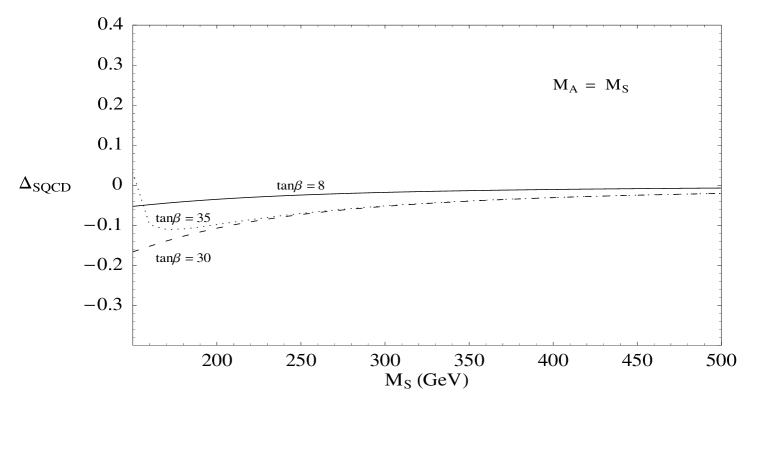
Figure 2: Exact numerical results for $\Delta_{SQCD}$ in $h^{0}\to b\overline{b}$ decay as a function of a common MSSM scale $M_{S}$ and for several values of $\tan\beta$

Finally, in order to show this decoupling numerically, we have studied a simple example where there is just one relevant MSSM scale, $M_{S}$. More specifically, we have chosen,

$$M_{S}=M_{\tilde{Q}}=M_{\tilde{D}}=\mu=A_{b}=M_{\tilde{g}}=M_{A},$$

which, in the limit $M_{S}\gg M_{Z}$, gives maximal mixing, $\theta_{\tilde{b}}\sim 45^{\circ}$. In Fig. 2 we show the numerical results for the exact one-loop SQCD corrections, as a function of this common MSSM mass scale $M_{S}$, and for several values of $\tan\beta$. We can see in this figure clearly the decoupling of $\Delta_{SQCD}$ with $M_{S}$. This decoupling goes as $1/M_{S}^{2}$, in agreement with our analytical result, and is delayed for large $\tan\beta$ values. The typical size of this correction is $\Delta_{SQCD}\leq-10\%$ for $M_{S}\geq 250\,GeV$. Notice that the sign of $\Delta_{SQCD}$ here is negative because of our choice of positive $\mu$ and $M_{\tilde{g}}$.

5 Comparing the decoupling behaviour of the various MSSM sectors in $h^{o}\to b\overline{b}$ decay

In this section we study and compare the decoupling behaviour of the different MSSM sectors that are relevant in the one-loop SQCD corrections to $h^{o}\to b\overline{b}$ decay. As we have discussed in the previous section, these are: the extra Higgs bosons, $H^{0}$, $A^{0}$, $H^{\pm}$, gluinos $\tilde{g}$ and sbottoms $\tilde{b}_{1,2}$. As regard to the Higgs sector, we have seen that there is no independent decoupling of these heavy $H^{0}$, $A^{0}$, $H^{\pm}$ Higgs bosons in $\Delta_{SQCD}$, unless the SQCD sector is also considered heavy. To illustrate this, we have ploted in Fig. 3 the numerical results of $\Delta_{SQCD}$ as a function of $M_{A}$ for several fixed values of the common SUSY scale $M_{S}=M_{\tilde{Q}}=M_{\tilde{D}}=\mu=A_{b}=M_{\tilde{g}}$ and for $\tan\beta=8$.

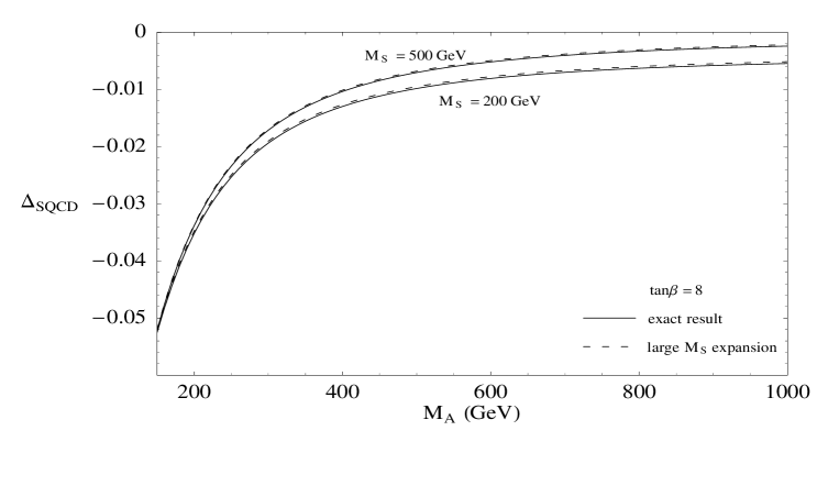
Figure 3: $\Delta_{SQCD}$ in $h^{0}\to b\overline{b}$ decay as a function of $M_{A}$ for fixed $M_{S}$

The fact that $\Delta_{SQCD}$ does not tend to zero for large $M_{A}$ but to a non-vanishing constant is a clear indication of a non-decoupling behaviour with $M_{A}$ for fixed $M_{S}$. Similarly, we have shown that there is no independent decoupling of the SQCD particles. That is, if we consider large values of the common SQCD scale $M_{S}$, while keeping $M_{A}$ fixed, $\Delta_{SQCD}$ approaches to a non-vanishing constant. This is illustrated clearly in Fig. 4.

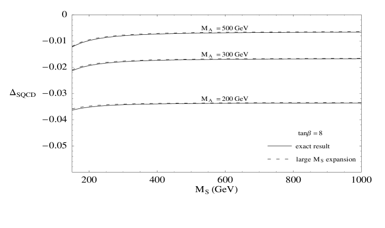
Figure 4: $\Delta_{SQCD}$ in $h^{0}\to b\overline{b}$ decay as a function of $M_{S}$ for fixed $M_{A}$

In these Figs. 3 and 4 we also show a comparison of the exact formula with our asymptotic expansion, valid for large $M_{S}$. We have seen that the large $M_{S}$ expansion provides a very good approximation to the exact result for most of the ($M_{S},\tan\beta$) parameter space, except for sufficiently low $M_{S}$ and large $\tan\beta$ values.

Next, we consider the independent decoupling of gluinos. By performing a second expansion in inverse powers of the gluino mass $M_{\tilde{g}}$, which is relevant in the heavy gluino limit $M_{\tilde{g}}\gg\tilde{M}_{S}\sim\mu\sim A_{b}\gg M_{Z}$, we get:

$${\Delta_{SQCD}}=\frac{\alpha_{s}}{3\pi}\Bigl{\{}\frac{2\mu}{{M_{\tilde{g}}}}({\tan\beta}+\cot\alpha)\left(1-\log\left(\frac{M^{2}_{\tilde{g}}}{\tilde{M}_{S}^{2}}\right)\right)$$

$$\qquad+\frac{2X_{b}}{{M_{\tilde{g}}}}\frac{M_{Z}^{2}}{\tilde{M}_{S}^{2}}\frac{\cos\beta\sin(\alpha+\beta)}{\sin\alpha}I_{3}^{b}-\frac{Y_{b}}{3{M_{\tilde{g}}}}\frac{m_{h}^{2}}{\tilde{M}_{S}^{2}}+{\mathcal{O}}\left(\frac{M^{2}}{{M_{\tilde{g}}^{2}}}\right)\Bigr{\}}.$$

This yields a very slow decoupling with $M_{\tilde{g}}$, due to the logarithmic dependence, and agrees with the previous exact numerical results of ref. [12]. For illustration we show in Fig. 5 our exact numerical results for $\Delta_{SQCD}$ as a function of $M_{\tilde{g}}$, for fixed $M_{A}=M_{S}$ value and for several $\tan\beta$ values.

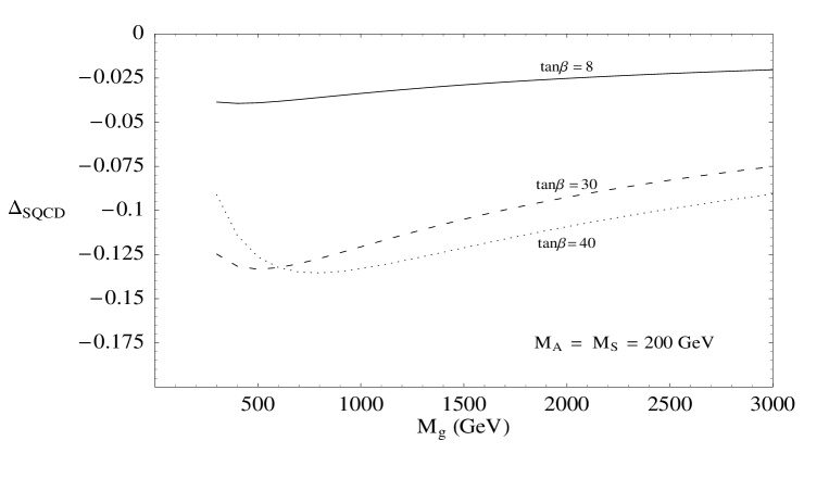
Figure 5: $\Delta_{SQCD}$ in $h^{0}\to b\overline{b}$ decay as a function of $M_{\tilde{g}}$

This very slow decoupling with $M_{\tilde{g}}$ may have important phenomenological consequences, in the large $\tan\beta$ regime, because the SQCD correction can reach sizeable values, even for large gluino masses. For instance, for $\tan\beta=30$ and $M_{\tilde{g}}=1TeV$ we get $\Delta_{SQCD}=-12\%$, which is not a small effect.

Finally, we have studied the independent decoupling of sbottoms. By performing an expansion in inverse powers of the average sbottom mass ${\tilde{M}_{S}}$, which is relevant in the heavy sbottoms limit, $\tilde{M}_{S}\gg M_{\tilde{g}}\sim\mu\sim A_{b}\gg M_{Z}$ we find the following result:

$${\Delta_{SQCD}}=\frac{\alpha_{s}}{3\pi}\left\{\frac{-2\mu M_{\tilde{g}}}{{\tilde{M}_{S}^{2}}}({\tan\beta}+\cot\alpha)\right.\left.+\frac{M_{Z}^{2}}{{\tilde{M}_{S}^{2}}}\frac{\cos\beta\sin(\alpha+\beta)}{\sin\alpha}I_{3}^{b}+{\mathcal{O}}\left(\frac{m_{b}^{2}}{{\tilde{M}_{S}^{2}}}\right)\right\}$$

It shows a fast decoupling behaviour as $\tilde{M}_{S}$ is taken large. This same behaviour is also manifest in our exact numerical results shown in Fig. 6

Figure 6: $\Delta_{SQCD}$ in $h^{0}\to b\overline{b}$ decay as a function of ${\tilde{M}_{S}}$

6 SUSY-QCD corrections to $H^{+}\rightarrow t\overline{b}$ in the decoupling limit

In this section we study the SUSY-QCD corrections to the partial decay width $\Gamma(H^{+}\rightarrow t\overline{b})$ at the one-loop level and to ${\cal O}$$(\alpha_{S})$. We will then analyze these corrections in the decoupling limit of large SUSY masses. We will present here just a short summary of the main numerical and analytical results, and refer the reader to ref. [7] for a more detailed study.

If all SUSY particles are heavy enough, $H^{+}$ decays dominantly into $t\overline{b}$ above the $t\overline{b}$ threshold. As in the case of $h^{0}\rightarrow b\overline{b}$, the dominant radiative corrections to $H^{+}\rightarrow t\overline{b}$ decay are the QCD corrections. At the one-loop level and to ${\cal O}$$(\alpha_{S})$ the corresponding partial width can be written as,

$$\Gamma_{1}(H^{+}\to t\overline{b})\equiv\Gamma_{0}(H^{+}\to t\overline{b})(1+2{\Delta_{QCD}}+2{\Delta_{SQCD}}),$$

where $\Gamma_{0}(H^{+}\to t\overline{b})$ is the tree-level width, $\Delta_{QCD}$ is the correction from standard QCD, and $\Delta_{SQCD}$ is the correction from SUSY-QCD. The standard QCD corrections were computed in ref. [19] and can be large ($+10\%$ to $-50\%$). The SUSY-QCD corrections were computed by using a diagrammatic approach in refs. [20, 21] and can be comparable or even larger than the standard QCD corrections in a large region of the SUSY parameter space.

At the one-loop level and to ${\cal O}(\alpha_{S})$ there are two type of diagrams that contribute to

$$\Delta_{SQCD}=\Delta_{SQCD}^{\rm loops}+\Delta_{SQCD}^{\rm CT},$$

as shown in Fig. 7.

Figure 7: One-loop SUSY diagrams contributing to ${\cal O}(\alpha_{S})$ to $H^{+}\to t\overline{b}$ decay

The triangle diagram, with exchange of sbottoms, stops and gluinos, contributes to $\Delta_{SQCD}^{\rm loops}$, whereas the bottom and top self-energy diagrams contribute to the counter-terms part $\Delta_{SQCD}^{\rm CT}$. The exact results in the on-shell scheme are summarized by,

$$\Delta_{SQCD}^{loops}=\frac{U_{t}}{D}\,H_{t}+\frac{U_{b}}{D}\,H_{b}\,,$$

$$\Delta_{SQCD}^{CT}=\frac{U_{t}}{D}\,\left(\frac{\delta m_{t}}{m_{t}}+\frac{1}{2}\,\delta Z_{L}^{b}+\frac{1}{2}\,\delta Z_{R}^{t}\,\right)+\frac{U_{b}}{D}\,\left(\frac{\delta m_{b}}{m_{b}}+\frac{1}{2}\,\delta Z_{L}^{t}+\frac{1}{2}\,\delta Z_{R}^{b}\,\right)\,,$$

where,

$$D = (M_{H^{+}}^{2}-m_{t}^{2}-m_{b}^{2})\,(m_{t}^{2}\cot^{2}\beta+m_{b}^{2}\tan^{2}\beta)-4m_{t}^{2}m_{b}^{2}\,,$$

$$U_{t} = (M_{H^{+}}^{2}-m_{t}^{2}-m_{b}^{2})\,m_{t}^{2}\cot^{2}\beta-2m_{t}^{2}m_{b}^{2}\,,$$

$$U_{b} = (M_{H^{+}}^{2}-m_{t}^{2}-m_{b}^{2})\,m_{b}^{2}\tan^{2}\beta-2m_{t}^{2}m_{b}^{2}\,,$$

$$H_{t} = -\frac{2\alpha_{s}}{3\pi}\,\frac{G_{ab}^{*}}{m_{t}\cot\beta}[m_{t}R^{(t)}_{1b}R^{(b)*}_{1a}(C_{11}-C_{12})+m_{b}R^{(t)}_{2b}R^{(b)*}_{2a}C_{12}$$

$$+M_{\tilde{g}}R^{(t)}_{2b}R^{(b*)}_{1a}C_{0}](m_{t}^{2},m_{H^{+}}^{2},M_{\tilde{g}}^{2},M_{\tilde{t}_{b}}^{2},M_{\tilde{b}_{a}}^{2})\,,$$

$$H_{b} = -\frac{2\alpha_{s}}{3\pi}\,\frac{G_{ab}^{*}}{m_{b}\tan\beta}[m_{t}R^{(t)}_{2b}R^{(b)*}_{2a}(C_{11}-C_{12})+m_{b}R^{(t)}_{1b}R^{(b)*}_{1a}C_{12}$$

$$+M_{\tilde{g}}R^{(t)}_{1b}R^{(b)*}_{2a}C_{0}](m_{t}^{2},m_{H^{+}}^{2},M_{\tilde{g}}^{2},M_{\tilde{t}_{b}}^{2},M_{\tilde{b}_{a}}^{2})\,,$$

and the counter-terms are given in the on-shell scheme by,

$$\frac{\delta m_{(t,b)}}{m_{(t,b)}}+\frac{1}{2}\,\delta Z_{L}^{(b,t)}+\frac{1}{2}\,\delta Z_{R}^{(t,b)}\, = \Sigma^{(t,b)}_{S}(m_{(t,b)}^{2})+\frac{1}{2}\Sigma^{(t,b)}_{L}(m_{(t,b)}^{2})-\frac{1}{2}\Sigma^{(b,t)}_{L}(m_{(b,t)}^{2})$$

$$-\frac{m_{t}^{2}}{2}\left[\Sigma^{t^{\prime}}_{L}(m_{t}^{2})+\Sigma^{t^{\prime}}_{R}(m_{t}^{2})+2\Sigma^{t^{\prime}}_{S}(m_{t}^{2})\right] - \frac{m_{b}^{2}}{2}\left[\Sigma^{b^{\prime}}_{L}(m_{b}^{2})+\Sigma^{b^{\prime}}_{R}(m_{b}^{2})+2\Sigma^{b^{\prime}}_{S}(m_{b}^{2})\right]$$

where,

$$\Sigma^{q}_{L}(p^{2}) = -\frac{2\alpha_{s}}{3\pi}\,|R^{(q)}_{1a}|^{2}B_{1}(p^{2},m^{2}_{\tilde{g}},m^{2}_{\tilde{q}_{a}})\,,$$

$$\Sigma^{q}_{R}(p^{2}) = -\frac{2\alpha_{s}}{3\pi}\,|R^{(q)}_{2a}|^{2}B_{1}(p^{2},m^{2}_{\tilde{g}},m^{2}_{\tilde{q}_{a}})\,,$$

$$\Sigma^{q}_{S}(p^{2}) = -\frac{2\alpha_{s}}{3\pi}\frac{m_{\tilde{g}}}{m_{q}}\,{\rm Re}(\,R^{(q)}_{1a}\,R^{(q)*}_{2a})B_{0}(p^{2},m^{2}_{\tilde{g}},m^{2}_{\tilde{q}_{a}})\,.$$

The $G_{ab}$ parametrize the $H^{+}\,\tilde{b}_{a}\,\tilde{t}_{b}$ couplings, and the $R^{(q)}$ are the rotation matrices that relate the interaction-eigenstate squarks to the mass-eigenstates. Their values in the MSSM can be found, for instance, in ref. [7]. The above result agrees with the original computation of refs. [20, 21].

In order to compute $\Delta_{SQCD}$ in the decoupling limit of large SUSY masses, we have considered all the soft-SUSY-breaking mass parameters and the $\mu$ parameter to be of the same order (collectively denoted by $M_{SUSY}$) and much heavier than the electroweak scale,

$$M_{SUSY}\sim M_{\tilde{Q}}\sim M_{\tilde{U}}\sim M_{\tilde{D}}\sim M_{\tilde{g}}\sim\mu\sim A_{t}\sim A_{b}\gg M_{EW},$$

and we have performed a systematic expansion in inverse powers of the large SUSY mass parameters. Notice that in this case it does not make sense to consider the alternative limit of large $M_{A}$, since this parameter provides the charged Higgs mass value and, therefore, it must be fixed. We have obtained analytical expansions for $\Delta_{SQCD}$ that include up to ${\cal O}(M_{EW}^{2}/{M^{2}_{SUSY}})$ corrections, for all the interesting limiting cases of maximal and minimal mixing, in both the stop and the sbottom sectors. For brevity, we do not present here the complete results, which can be found in ref. [7], and we just show the most relevant result, that is, the dominant term in this expansion for the particular choice of maximal mixing. Thus, for $\theta_{\tilde{b},\tilde{t}}\sim 45^{o}$ and $\tilde{M}_{S}^{2}\equiv\frac{1}{2}(M_{\tilde{b}_{1}}^{2}+M_{\tilde{b}_{2}}^{2})\equiv\frac{1}{2}(M_{\tilde{t}_{1}}^{2}+M_{\tilde{t}_{2}}^{2})$ we get:

$${\Delta_{SQCD}}=\frac{\alpha_{s}}{3\pi}\left\{\frac{-{\mu M_{\tilde{g}}}}{{\tilde{M}_{S}^{2}}}\left(\tan\beta+\cot\beta\right)f_{1}(R)+{\cal{O}}\left(\frac{M_{EW}^{2}}{{\tilde{M}_{S}^{2}}}\right)\right\}$$

This leading term does not vanish in the heavy SUSY particle limit and, therefore, there is no decoupling of stops, sbottoms and gluinos in the $\Gamma(H^{+}\to t\overline{b})$ decay width to one-loop level. This can be seen clearly, for instance, for the simplest case of equal mass scales, $\mu=M_{\tilde{g}}=\tilde{M}_{S}$, where $f_{1}(R)=1$. This leading term, when expressed in terms of an effective coupling of $H^{+}$ to $b\overline{t}$ is in agreement with the previous results of refs. [16, 17] that were obtained in the zero external momentum approximation by using an effective Lagrangian approach. We see in this result the enhancement of $\Delta_{SQCD}$ by $\tan\beta$, so that this non-decoupling effect can be numerically important for large $\tan\beta$ values. As in the case of $h^{0}$, the sign of the SQCD correction is determined by the sign of $M_{\tilde{g}}$ and $\mu$. We have obtained similar results for the case of minimal mixing, as can be seen in [7].

Finally, in order to illustrate this non-decoupling behaviour numerically, we present in Fig. 8 the $\Delta_{SQCD}$ correction as a function of a common SUSY mass scale $M_{S}=M_{\tilde{Q}}=M_{\tilde{U}}=M_{\tilde{D}}=M_{\tilde{g}}=A_{b}=A_{t}=\mu$. The Higgs mass has been fixed to $m_{H^{+}}=250\,GeV$, and several values of $\tan\beta$ have been considered. The fact that $\Delta_{SQCD}$ tends to a non-vanishing value for very large $M_{S}$ shows precisely this non-decoupling effect. The correction is quite sizeable, even for a very heavy SUSY spectrum. This is particularly noticeable for large $\tan\beta$.

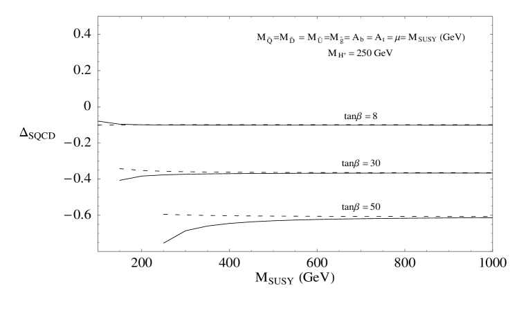
Figure 8: $\Delta_{SQCD}$ in $H^{+}\rightarrow t\overline{b}$ decay as a function of the common SUSY scale $M_{S}$

In addition, we have proved the independent decoupling of the gluinos and squarks whenever they are considered separately very heavy as compared to the electroweak scale. Futhermore, the decoupling of gluinos is much slower than the decoupling of squarks due again to the logarithmic dependence on the gluino mass. In Fig. 9 we show the exact numerical results for $\Delta_{SQCD}$ as a function of the gluino mass and for $M_{\tilde{Q}}=M_{\tilde{U}}=M_{\tilde{D}}=A_{b}=A_{t}=\mu=1\,TeV$ and $m_{H^{+}}=250\,GeV$. We see clearly the very slow decoupling of the correction with the gluino mass and notice the large size of $\Delta_{SQCD}$, specially for large $\tan\beta$. For instance, if $\tan\beta=30$ and $M_{\tilde{g}}=2$ TeV we get $\Delta_{SQCD}=-40\%$. Notice that the size can be so large that the validity of the perturbative expansion can be questionable. We refer the reader to refs. [16, 17] where this subject is studied and some techniques of resummation for a better convergence of the series are proposed.

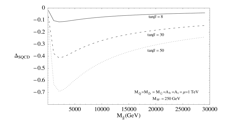
Figure 9: $\Delta_{SQCD}$ in $H^{+}\rightarrow t\overline{b}$ decay as a function of $M_{\tilde{g}}$

7 SUSY-QCD corrections to $t\rightarrow W^{+}b$ in the decoupling limit

In this section we briefly comment on the SUSY-QCD corrections to $t\rightarrow W^{+}b$ at the one-loop level and to ${\cal O}(\alpha_{S})$, and we study them in the decoupling limit. These radiative corrections were studied in the context of the MSSM in ref. [22] and are known to be important for some regions of the MSSM parameter space. The standard QCD corrections are also known to be important and give a $\sim-10\%$ reduction in $\Gamma(t\rightarrow W^{+}b)$ [23]. The Feynman diagrams that contribute to the SQCD corrections are shown in Fig. 10.

Figure 10: One-loop SUSY diagrams contributing to ${\cal O}(\alpha_{S})$ in $t\rightarrow W^{+}b$ decay

The size of the SQCD corrections has been estimated to range between $-5\%$ and $-10\%$ and are quite insensitive to $\tan\beta$ [22]. In contrast, the SUSY-Electroweak corrections that range between $-1\%$ and $-10\%$ are known to grow with $\tan\beta$ [24].

In order to analyze the decoupling limit in this observable we have chosen the simplest case with just one SUSY scale, $M_{S}$, which is considered very large as compared to the electroweak scale, $M_{EW}$,

$$M_{\tilde{Q}}=M_{\tilde{U}}=M_{\tilde{D}}=A_{t}=A_{b}=\mu=M_{\tilde{g}}=M_{S}\gg M_{EW}\,.$$

After performing an expansion of $\Delta_{SQCD}$ (we use here an analogous notation as in previous sections) in inverse powers of $M_{S}$ we have obtained the following result for the dominant contribution,

$$\Delta_{SQCD} = -\frac{\alpha_{s}}{3\pi}\frac{m_{t}^{2}}{M_{S}^{2}}\left(\frac{1}{6}+\frac{1}{24}(1-\cot\beta)^{2}+\frac{1}{6}(1-\cot\beta)\right)+{\cal{O}}\left(\frac{m_{t}m_{W},m_{W}^{2},...}{M_{S}^{2}}\right)$$

From this result, we conclude that there is decoupling as $M_{S}$ becomes large in the SQCD corrections to the dominant top decay, $t\rightarrow W^{+}b$, and this decoupling which behaves as $(m_{t}^{2}/M_{S}^{2})$ is not delayed. Indeed, we see in the previous equation that these corrections are not enhanced by $\tan\beta$. Thus, we do not expect relevant indirect signals from a heavy SUSY-QCD sector in this decay channel.

8 Conclusions

In this work we have studied the one-loop SQCD corrections to the partial widths of $h^{0}\rightarrow b\overline{b}$, $H^{+}\rightarrow t\overline{b}$ and $t\rightarrow W^{+}b$ decays, in the limit of large SUSY masses. In order to understand analytically the behavior of the SQCD corrections in this limit, we have performed expansions of the one-loop partial widths that are valid for large values of the SUSY mass parameters compared to the electroweak scale. We have shown that for the SUSY mass parameters and $M_{A}$ large and all of the same order, the SQCD corrections in $h^{0}\rightarrow b\overline{b}$ decay decouple like the inverse square of these mass parameters, and the one-loop partial width $\Gamma(h^{0}\rightarrow b\overline{b})$ tends to its SM value. In this case the effective low energy theory that one obtains after integrating out all the heavy non-standard modes of the MSSM is precisely the SM. However, if the mass parameters are not all of the same size, then this behavior can be modified. If $M_{A}$ is light, then the SQCD corrections to the $\Gamma(h^{0}\rightarrow b\overline{b})$ decay width do not decouple in the limit of large SUSY mass parameters. We have also presented and discussed here a similar non-decoupling SQCD correction to the $\Gamma(H^{+}\rightarrow t\overline{b})$ decay width. Given the closely related structure of the various Higgs bosons couplings to the SM fermions, one expects that similar SUSY non-decoupling effects will appear as well in other decay channels such as $H^{0}\rightarrow b\overline{b}$, $A^{0}\rightarrow b\overline{b}$ and $t\rightarrow H^{+}b$. In the limit of large SUSY mass parameters and light $M_{A}$ the effective low-energy theory, valid at the electroweak scale, should contain two full Higgs doublets with Higgs-fermion couplings of the general type-III model [25] that have no restrictions (other than those imposed by the SM symmetries), since supersymmetry is not anymore a symmetry of this low-energy theory. The particular values of the couplings in this low-energy effective Lagrangian are generated by integrating out all the heavy SUSY particles from the original MSSM Lagrangian, and they can be computed [26]. These non-decoupling SQCD corrections can be of phenomenological interest at present and future colliders. In particular they can provide some clues in the indirect search of a heavy SUSY spectrum at the LHC [27].

We have also examined, in Higgs decays, some special cases in which there is a hierarchy among the SUSY mass parameters. In the case of maximal squark mixing with $M_{S}$ large and the other SUSY mass parameters and $M_{A}$ of order a common mass scale $M$ (chosen such that $M_{EW}\ll M\ll M_{S}$), the SQCD corrections decouple like $M^{2}/M_{S}^{2}$. Second, we examined the case of a large gluino mass with the other SUSY mass parameters of order a common mass scale $M$ (chosen such that $M_{EW}\ll M\ll M_{\tilde{g}}$). In this case we found that the SQCD corrections decouple more slowly, like $(M/M_{\tilde{g}})\log(M^{2}_{\tilde{g}}/M_{S}^{2})$.

Finally we have studied the dominant decay of the top quark, in the decoupling limit of large SUSY mass parameters, and we have found that the SQCD corrections decouple as ${\cal O}(\frac{m_{t}^{2}}{M_{S}^{2}})$. It will be, therefore, very difficult to look for indirect heavy SUSY signals in this channel.

Acknowledgments

M.J.H. wish to thank Howard E. Haber and the Organizing Committee for the kind invitation to give a talk at this Symposium and for the enjoyable atmosphere at this interesting conference. S.P. acknowledges H.E. Haber for the invitation to attend this Symposium. This work has been supported in part by the Spanish Ministerio de Educacion y Cultura under project CICYT AEN97-1678. S.P. has been partially supported by the U.S. Department of Energy under contract DE-FG03-92ER40689 and by Ramon Areces Foundation. S.R. has been partially supported by the European Union through contract ERBFMBICT972474. H.E.H. is supported in part by the U.S. Department of Energy under contract DE-FG03-92ER40689. Fermilab is operated by Universities Research Association Inc. under contract no. DE-AC02-76CH03000 with the U.S. Department of Energy.

References

- [1] H. E. Haber and Y. Nir, Nucl. Phys. B335, 363 (1990); H. E. Haber, in Proceedings of the US–Polish Workshop, Warsaw, Poland, September 21–24, 1994, edited by P. Nath, T. Taylor, and S. Pokorski (World Scientific, Singapore, 1995) pp. 49–63.
- [2] A. Dobado, M. J. Herrero and S. Peñaranda, Eur. Phys. J. C7, 313 (1999); Eur. Phys. J. C12, 673 (2000); Eur. Phys. J. C17, 487 (2000).
- [3] T. Appelquist and J. Carazzone, Phys. Rev. D11, 2856 (1975).
- [4] M. Carena, S. Mrenna and C. E. M. Wagner, Phys. Rev. D60, 075010 (1999); Phys. Rev. D62, 055008 (2000).
- [5] M. Carena, J. S. Conway, H. E. Haber and J. D. Hobbs, Report of the Tevatron Higgs Working Group, hep-ph/0010338
- [6] H. E. Haber, M. J. Herrero, H. E. Logan, S. Penaranda, S. Rigolin and D. Temes, Phys. Rev. D 63, 055004 (2001) ,
- [7] M. J. Herrero, S. Peñaranda and D. Temes, SUSY-QCD decoupling properties in decay, FTUAM 00/20; IFT-UAM/CSIC 00/42
- [8] J. F. Gunion, H. E. Haber, G. Kane and S. Dawson, The Higgs Hunter’s Guide (Addison–Wesley, Reading, MA, 1990) [errata: hep-ph/9302272].
- [9] H. E. Haber, Nonminimal Higgs sector: The decoupling limit and its phenomenological implications (1994), hep-ph/9501320.
- [10] E. Braaten and J. P. Leveille, Phys. Rev. D22, 715 (1980); N. Sakai, Phys. Rev. D22, 2220 (1980); T. Inami and T. Kubota, Nucl. Phys. B179, 171 (1981).
- [11] A. Dabelstein, Nucl. Phys. B456, 25 (1995).
- [12] J. A. Coarasa, R. A. Jiménez and J. Solà, Phys. Lett. B389, 312 (1996).
- [13] L. J. Hall, R. Rattazzi and U. Sarid, Phys. Rev. D50, 7048 (1994); R. Hempfling, Phys. Rev. D49, 6168 (1994); M. Carena, M. Olechowski, S. Pokorski and C. E. M. Wagner, Nucl. Phys. B426, 269 (1994).
- [14] D. M. Pierce, J. A. Bagger, K. Matchev and R.-J. Zhang, Nucl. Phys. B491, 3 (1997).
- [15] S. Heinemeyer, W. Hollik and G. Weiglein, Eur. Phys. J. C16, 139 (2000).
- [16] M. Carena, D. Garcia, U. Nierste and C. E. M. Wagner, Nucl. Phys. B577, 88 (2000).
- [17] H. Eberl, K. Hidaka, S. Kraml, W. Majerotto and Y. Yamada, Phys. Rev. D62 055006 (2000).
- [18] W. Hollik, in Precision Tests of the Standard Electroweak Model, edited by P. Langacker (World Scientific, Singapore, 1995), p. 37–116.
- [19] A. Mendez and A. Pomarol, Phys. Lett. B252, 461 (1990); C. S. Li and R.Oakes, Phys. Rev. D43, 855 (1991); A. Djouadi and P. Gambino, Phys. Rev. D51, 218 (1995).
- [20] R. A. Jimenez and J. Sola, Phys. Lett. B389, 53 (1996).
- [21] A. Bartl, H. Eberl, K. Hidaka, T. Kon, W. Majerotto and Y. Yamada, Phys. Lett. B378, 167 (1996).
- [22] A. Dabelstein, W. Hollik, R. A. Jimenez, C. Junger and J. Sola, Nucl. Phys. B454, 75 (1995).
- [23] M. Jezabek and J. H. Kühn, Nucl. Phys. B314, 1 (1989); ibid B320, 20 (1989); C. S. Li, R. J. Oakes and T. C. Yuan, Phys. Rev. D43 3759 (1991); A. Denner and T. Sack, Z. Phys. C46 653 (1990); Nucl. Phys. B358, 46 (1991).
- [24] D. Garcia, W. Hollik, R. A. Jimenez and J. Sola, Nucl. Phys. B427, 53 (1994); J. M. Yang and C. S. Li, Phys. Lett. 320 117 (1994).
- [25] W. S. Hou, Phys. Lett. B296, 179 (1992) ; D. Chang, W. S. Hou and W. Y. Keung, Phys. Rev. D48, 217 (1993); D. Atwood, L. Reina and A. Soni, Phys. Rev. D55, 3156 (1997).
- [26] A. Dobado, M. J. Herrero and D. Temes, in progress.
- [27] A. M. Curiel, M. J. Herrero, D. Temes and J. F. de Troconiz, in progress.