VARIOUS SOLUTIONS OF THE ATMOSPHERIC NEUTRINO DATA

Various solutions of the atmospheric neutrino data are reviewed. Apart from orthodox two flavor $\nu_{\mu}\leftrightarrow\nu_{\tau}$ oscillations and three flavor oscillations, there are still possibilities, such as four flavor oscillations with the (2+2)- and (3+1)- schemes, a neutrino decay scenario and decoherence, which give a good fit to the data.

1 Introduction

It has been known that the atmospheric neutrino anomaly $\!{}^{{\bf?},{\bf?},{\bf?},{\bf?},{\bf?},{\bf?},{\bf?},{\bf?},{\bf?},{\bf?},{\bf?}}$ can be accounted for by dominant $\nu_{\mu}\leftrightarrow\nu_{\tau}$ oscillations with almost maximal mixing, and the zenith angle dependence of atmospheric neutrinos has been analyzed by many theorists $\!{}^{{\bf?}}$ as well as by experimentalists $\!{}^{{\bf?},{\bf?},{\bf?},{\bf?},{\bf?},{\bf?},{\bf?}}$. On the other hand, the solar neutrino observations $\!{}^{{\bf?},{\bf?},{\bf?},{\bf?},{\bf?},{\bf?}}$ and the LSND experiment $\!{}^{{\bf?},{\bf?}}$ also suggest neutrino oscillations. $\Delta m^{2}_{\mbox{\rm\footnotesize atm}}$, $\Delta m^{2}_{\odot}$ and $\Delta m^{2}_{\mbox{\rm{\scriptsize LSND}}}$ (the mass squared differences suggested by the atmospheric neutrino anomaly, the solar neutrino deficit and the LSND data) have different orders of magnitudes and there have been a lot of works to analyze the atmospheric neutrino data from the view point of ordinary oscillations due to mass with two, three and four flavors as well as exotic scenarios. In this talk I will review the status of various scenarios which have been proposed to explain the atmospheric neutrino problem.

2 Neutrino oscillations due to mass

2.1 Neutrino oscillations with two flavors

The most up-to-date result of the two flavor analysis of $\nu_{\mu}\leftrightarrow\nu_{\tau}$ with 1289 day data has been given by McGrew $\!{}^{{\bf?}}$ and the allowed region of the oscillation parameters at 90%CL is

$$0.88< \sin^{2}2\theta_{\mbox{\rm\footnotesize atm}} \leq 1$$

$$1.6\times 10^{-3}{\rm eV}^{2}< \Delta m_{\mbox{\rm\footnotesize atm}}^{2} <4\times 10^{-3}{\rm eV}^{2}.$$

On the other hand, two flavor analysis of $\nu_{\mu}\leftrightarrow\nu_{s}$ has been done by the Superkamiokande group using the data of neutral current enriched multi-ring events, high energy partially contained events and upward going $\mu$’s, and they have excluded the two flavor oscillation $\nu_{\mu}\leftrightarrow\nu_{s}$ at 99%CL $\!{}^{{\bf?}}$.

2.2 Neutrino oscillations with three flavors

The flavor eigenstates are related to the mass eigenstates by the $3\times 3$ MNS mixing matrix:

$$\left(\begin{array}[]{ccc}U_{e1}&U_{e2}&U_{e3}\\ U_{\mu 1}&U_{\mu 2}&U_{\mu 3}\\ U_{\tau 1}&U_{\tau 2}&U_{\tau 3}\end{array}\right)=\left(\begin{array}[]{ccc}c_{12}c_{13}&s_{12}c_{13}&s_{13}e^{-i\delta}\\ -s_{12}c_{23}-c_{12}s_{23}s_{13}e^{i\delta}&c_{12}c_{23}-s_{12}s_{23}s_{13}e^{i\delta}&s_{23}c_{13}\\ s_{12}s_{23}-c_{12}c_{23}s_{13}e^{i\delta}&-c_{12}s_{23}-s_{12}c_{23}s_{13}e^{i\delta}&c_{23}c_{13}\\ \end{array}\right),$$ (7)

and without loss of generality I assume $|\Delta m_{21}^{2}|<|\Delta m_{32}^{2}|<|\Delta m_{31}^{2}|$ where $\Delta m^{2}_{ij}\equiv m^{2}_{i}-m^{2}_{j}$, $m_{j}^{2}(j=1,2,3)$ are the mass squared for the mass eigenstates. Since there are only two independent mass squared differences, it is impossible to account for the solar neutrino deficit, the atmospheric neutrino anomaly and LSND (the only nontrivial possibility is to take $\Delta m^{2}_{21}=\Delta m^{2}_{\mbox{\rm\footnotesize atm}}$ and $\Delta m^{2}_{32}=\Delta m^{2}_{\mbox{\rm{\scriptsize LSND}}}$ and to try to explain the solar neutrino problem with the energy independent solution; It turns out, however, that the main oscillation channel in the atmospheric neutrinos in this case is $\nu_{\mu}\leftrightarrow\nu_{e}$ and therefore the zenith angle dependence of the atmospheric neutrino data cannot be explained). So I have to give up an effort to explain LSND and I have to take $\Delta m^{2}_{21}=\Delta m^{2}_{\odot}$ and $\Delta m^{2}_{32}=\Delta m^{2}_{\mbox{\rm{\scriptsize atm}}}$. Under the present assumption it follows $\Delta m^{2}_{\rm atm}=\Delta m^{2}_{32}$ $\gg$$\Delta m^{2}_{21}=\Delta m^{2}_{\odot}$ and I have a large hierarchy between $\Delta m^{2}_{21}$ and $\Delta m^{2}_{32}$. If $|\Delta m^{2}_{\odot}L/4E|\ll 1$ then from a hierarchical condition I have the oscillation probability

$$P(\bar{\nu}_{e}\rightarrow\bar{\nu}_{e})=1-\sin^{2}2\theta_{13}\Delta_{32},$$

where $\Delta_{jk}\equiv\sin^{2}(\Delta m_{jk}^{2}L/4E)$, so if $\Delta m^{2}_{\rm atm}>2\times 10^{-3}$eV² then the CHOOZ reactor data $\!{}^{{\bf?}}$ force us to have either $\theta_{13}\simeq 0$ or $\theta_{13}\simeq\pi/2$. On the other hand, the solar oscillation probability in the three flavor framework is related to that in the two flavor case by $\!{}^{{\bf?}}$

$$P^{(3)}(\nu_{e}\rightarrow\nu_{e};A(x))=c_{13}^{4}P^{(2)}(\nu_{e}\rightarrow\nu_{e};c_{13}^{2}A(x))+s_{13}^{4},$$

where $A(x)$ stands for the matter effect. To account for the solar neutrino deficit, therefore, $|s_{13}|$ cannot be too large, so it follows that $|\theta_{13}|\ll 1$ and the MNS mixing matrix $U$ becomes

$$U\simeq\left(\begin{array}[]{ccc}c_{\odot}&s_{\odot}&\epsilon\\ -s_{\odot}/\sqrt{2}-c_{\odot}/\sqrt{2}&c_{\odot}/\sqrt{2}-s_{\odot}/\sqrt{2}&1/\sqrt{2}\\ s_{\odot}/\sqrt{2}-c_{\odot}/\sqrt{2}&-c_{\odot}/\sqrt{2}-s_{\odot}/\sqrt{2}&1/\sqrt{2}\\ \end{array}\right),$$ (11)

which indicates that the solar neutrino problem is explained by oscillations half of which is $\nu_{e}\rightarrow\nu_{\mu}$ and the other is $\nu_{e}\rightarrow\nu_{\tau}$, and that the atmospheric neutrino anomaly is accounted for by oscillations of almost 100% $\nu_{\mu}\rightarrow\nu_{\tau}$ ($|\epsilon|\equiv|\theta_{13}|\ll 1$).

On the other hand, if $\Delta m^{2}_{\rm atm}<$$2\times 10^{-3}$eV², then $\theta_{13}$ can be relatively large (This possibility gives a bad fit to the atmospheric neutrino data but is not excluded at $4\sigma$CL yet). From the combined three flavor analysis of the Superkamiokande atmospheric neutrino data with the CHOOZ data, it has been shown $\!{}^{{\bf?},{\bf?}}$ that $|\theta_{13}|\raisebox{0.85358pt}{\em$\,<$}\raisebox{-3.69885pt}{\em$\sim\,$}\pi/12$ is allowed at 99%CL. Hence the probability

$$P(\nu_{\mu}\rightarrow\nu_{e})=s^{2}_{23}\sin^{2}2\theta_{13}\Delta_{32}$$

of appearance of $\nu_{e}$ can be relatively large and there is a chance in long baseline experiments to observe $\nu_{e}$ in this case.

2.3 Neutrino oscillations with four flavors

To explain the solar, atmospheric and LSND data within the framework of neutrino oscillations, it is necessary to have at least four kinds of neutrinos. In the case of four neutrino schemes there are two distinct types of mass patterns. One is the so-called (2+2)-scheme (Fig. 1(a)) and the other is the (3+1)-scheme (Fig. 1(b) or (c)). Depending on the type of the two schemes, phenomenology is different.

Figure 1: Mass patterns of four neutrino schemes. (a) corresponds to (2+2)-scheme, where either ($|\Delta m^{2}_{21}|=\Delta m^{2}_{\odot}$, $|\Delta m^{2}_{43}|=\Delta m^{2}_{\mbox{\rm\footnotesize atm}}$) or ($|\Delta m^{2}_{43}|=\Delta m^{2}_{\odot}$, $|\Delta m^{2}_{21}|=\Delta m^{2}_{\mbox{\rm\footnotesize atm}}$). (b) and (c) are (3+1)-scheme, where $|\Delta m^{2}_{41}|=\Delta m^{2}_{\mbox{\rm{\scriptsize LSND}}}$ and either ($|\Delta m^{2}_{21}|=\Delta m^{2}_{\odot}$, $|\Delta m^{2}_{32}|=\Delta m^{2}_{\mbox{\rm\footnotesize atm}}$) or ($|\Delta m^{2}_{32}|=\Delta m^{2}_{\odot}$, $|\Delta m^{2}_{21}|=\Delta m^{2}_{\mbox{\rm\footnotesize atm}}$) is satisfied.

The atmospheric neutrino data were analyzed by Refs. $\!{}^{{\bf?},{\bf?}}$ with the (2+2)-scheme. Here I assume the mass pattern in Fig. 1(a) with $\Delta m^{2}_{21}=\Delta m^{2}_{\odot}$ and $\Delta m^{2}_{43}=\Delta m^{2}_{\mbox{\rm\footnotesize atm}}$. I also assume $U_{e3}=U_{e4}=0$, which is justified from the Bugey reactor constraint $|U_{e3}|^{2}+|U_{e4}|^{2}\ll 1$, and $\Delta m^{2}_{\odot}=0$, since $|\Delta m^{2}_{\odot}L/2E|\ll 1$ in the atmospheric neutrino oscillations. I take the reference value $\Delta m^{2}_{\mbox{\rm{\scriptsize LSND}}}=0.3$ eV² so that the result with large $|U_{\mu 3}|^{2}+|U_{\mu 4}|^{2}$ do not contradict with the CDHSW constraint

$$1-P(\nu_{\mu}\rightarrow\nu_{\mu}) = 4(|U_{\mu 3}|^{2}+|U_{\mu 4}|^{2})(1-|U_{\mu 3}|^{2}-|U_{\mu 4}|^{2})\Delta_{32}$$

$$\leq \sin^{2}2\theta_{\mbox{\rm\scriptsize CDHSW}}(\Delta m^{2}_{32})\Delta_{32},$$

where $\sin^{2}2\theta_{\mbox{\rm\scriptsize CDHSW}}(\Delta m^{2})$ stand for the value of the boundary of the excluded region of CDHSW $\!{}^{{\bf?}}$ in the two flavor analysis as a function of $\Delta m^{2}$. With these assumptions, $\nu_{e}$ decouples from other three neutrinos, and the problem is reduced to the three flavor neutrino analysis among $\nu_{\mu}$, $\nu_{\tau}$, $\nu_{s}$ and the reduced MNS matrix is

$$\widetilde{U} \equiv \left(\begin{array}[]{ccc}U_{\mu 2}&U_{\mu 3}&U_{\mu 4}\\ U_{\tau 2}&U_{\tau 3}&U_{\tau 4}\\ U_{s2}&U_{s3}&U_{s4}\end{array}\right)=e^{i({\pi\over 2}-\theta_{34})\lambda_{7}}D^{-1}e^{i\theta_{24}\lambda_{5}}D~{}e^{i(\theta_{23}-{\pi\over 2})\lambda_{2}},$$ (15)

with $D\equiv{\rm diag}\left(e^{i\delta_{1}/2},1,e^{-i\delta_{1}/2}\right)$ ($\lambda_{j}$ are the $3\times 3$ Gell-Mann matrices) is the reduced $3\times 3$ MNS matrix. This MNS matrix $\widetilde{U}$ is obtained by substitution $\theta_{12}\rightarrow\theta_{23}-\pi/2$, $\theta_{13}\rightarrow\theta_{24}$, $\theta_{12}\rightarrow\pi/2-\theta_{34}$, $\delta\rightarrow\delta_{1}$ in the standard parametrization in Ref. $\!{}^{{\bf?}}$. $\theta_{34}$ corresponds to the mixing of $\nu_{\mu}\leftrightarrow\nu_{\tau}$ and $\nu_{\mu}\leftrightarrow\nu_{s}$, while $\theta_{23}$ is the mixing of the contribution of $\displaystyle\sin^{2}(\Delta m^{2}_{\mbox{\rm\footnotesize atm}}L/4E)$ and $\displaystyle\sin^{2}(\Delta m^{2}_{\mbox{\rm{\scriptsize LSND}}}L/4E)$ in the oscillation probability. The allowed region at 90%CL of the atmospheric neutrino data is roughly given by $\!{}^{{\bf?}}$ $30^{\circ}\raisebox{0.85358pt}{\em$\,<$}\raisebox{-3.69885pt}{\em$\sim\,$}\theta_{24}\raisebox{0.85358pt}{\em$\,<$}\raisebox{-3.69885pt}{\em$\sim\,$}55^{\circ}$, $0\leq\theta_{23}\raisebox{0.85358pt}{\em$\,<$}\raisebox{-3.69885pt}{\em$\sim\,$}30^{\circ}$, $-90^{\circ}\theta_{23}\raisebox{0.85358pt}{\em$\,<$}\raisebox{-3.69885pt}{\em$\sim\,$}90^{\circ}$. The reasons that the (2+2)-scheme is consistent with the recent Superkamiokande data are because both solar and atmospheric neutrinos have hybrid of active and sterile oscillations in this scheme and because there is a constant term in the surviving probability

$$P(\nu_{\mu}\rightarrow\nu_{\mu})=1-4|U_{\mu 3}|^{2}|U_{\mu 4}|^{2}\Delta_{43}-2(|U_{\mu 3}|^{2}+|U_{\mu 4}|^{2})(1-|U_{\mu 3}|^{2}-|U_{\mu 4}|^{2})$$

due to nonvanishing contribution of $\sin^{2}(\Delta m^{2}_{\mbox{\rm{\scriptsize LSND}}}L/4E)$, where I have averaged over rapid oscillations: $\sin^{2}({\Delta m^{2}_{\mbox{\rm{\scriptsize LSND}}}L/4E})\rightarrow 1/2$.

On the other hand, it has been shown in Refs. $\!{}^{{\bf?},{\bf?}}$ using older data of LSND $\!{}^{{\bf?}}$ that the (3+1)-scheme is inconsistent with the Bugey reactor data $\!{}^{{\bf?}}$ and the CDHSW disappearance experiment $\!{}^{{\bf?}}$ of $\nu_{\mu}$. However, in the final result the allowed region has shifted to the lower value of $\sin^{2}2\theta$ and it was shown $\!{}^{{\bf?}}$ that there are four isolated regions $\Delta m^{2}_{\mbox{\rm{\scriptsize LSND}}}\simeq$0.3, 0.9, 1.7, 6.0 eV² which satisfy both the constraints of Bugey and CDHSW and the LSND data at 99%CL. The case of $\Delta m^{2}_{\mbox{\rm{\scriptsize LSND}}}$=0.3 eV² turns out to be excluded by the Superkamiokande atmospheric neutrino data at 6.9$\sigma$CL $\!{}^{{\bf?}}$. For the other three values of $\Delta m^{2}_{\mbox{\rm{\scriptsize LSND}}}$, I have $U_{e4}\simeq U_{\mu 4}\simeq 0$ and this case is reduced to the analysis in the (2+2)-scheme with $\theta_{23}=0$. The allowed region at 90%CL is given roughly by $-\pi/4\raisebox{0.85358pt}{\em$\,<$}\raisebox{-3.69885pt}{\em$\sim\,$}\theta_{34}\raisebox{0.85358pt}{\em$\,<$}\raisebox{-3.69885pt}{\em$\sim\,$}\pi/4$, $0.8\raisebox{0.85358pt}{\em$\,<$}\raisebox{-3.69885pt}{\em$\sim\,$}\sin^{2}2\theta_{24}\leq 1$, where $\theta_{34}$ and $\theta_{24}$ stand for the mixing of $\nu_{\mu}\leftrightarrow\nu_{\tau}$ and $\nu_{\mu}\leftrightarrow\nu_{s}$ and the mixing of atmospheric neutrino oscillations, respectively.

3 Exotic solutions

Apart from ordinary oscillations due to mass, several possibilities have been proposed which predict different behaviors of the oscillation probability as a function of the neutrino energy. Those include violation of the equivalence principle $\!{}^{{\bf?}}$, violation of the Lorentz invariance $\!{}^{{\bf?}}$, presence of torsion $\!{}^{{\bf?}}$, flavor changing neutral current interactions $\!{}^{{\bf?}}$, neutrino decays $\!{}^{{\bf?},{\bf?}}$ decoherence of the neutrino beam $\!{}^{{\bf?}}$, large extra dimensions $\!{}^{{\bf?}}$, etc. As in the case of test of sterile oscillations, the zenith angle dependence (or the up-down asymmetry) of the high energy atmospheric neutrino data give strong constraints on these exotic scenarios. In the case of violation of the equivalence principle or the Lorentz invariance, the $\nu_{\mu}$ disappearance probability $P_{\mu\mu}\equiv P(\nu_{\mu}\rightarrow\nu_{\mu};L)$ is given by

$$P_{\mu\mu}=1-\sin^{2}2\theta\sin^{2}\left({\mbox{\rm const}}\cdot EL\right)$$

and in the case of flavor changing neutral current interactions

$$P_{\mu\mu}=1-\sin^{2}2\theta\sin^{2}\left({\mbox{\rm const}}\cdot L\right).$$

Both possibilities are strongly disfavored (See Fig. 3 which is taken from Ref. $\!{}^{{\bf?}}$).

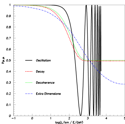
Figure 2: $\chi^{2}$ of the SK atmospheric neutrino data as a function of index $n$ ($1-P_{\mu\mu}=\sin^{2}2\theta\sin^{2}({\mbox{\rm const}}E^{n}L)$). $n=-1$ corresponds to ordinary oscillations due to mass.

Figure 3: Behaviors of the surviving probability $P(\nu_{\mu}\rightarrow\nu_{\mu})$ as a function of $L/E$ for scenarios of oscillations, decay, decoherence and extra dimensions.

In the case of neutrino decays, which were originally introduced to try to explain the solar, atmospheric neutrinos and LSND within the three flavor framework with two oscillation parameters $\Delta m^{2}_{21}$, $\Delta m^{2}_{32}$ and one neutrino decay constant $\alpha$, the disappearance probability is

$$P_{\mu\mu}=\sin^{4}\theta+\cos^{4}\theta\exp(-\alpha L/E)+{1\over 2}\sin^{2}2\theta\exp(-\alpha L/2E)\cos\left(\Delta m^{2}L/2E\right)$$

which has the following two extreme cases:

$$P_{\mu\mu} = \sin^{4}\theta+\cos^{4}\theta\exp(-\alpha L/E)\qquad\qquad\Delta m^{2}\rightarrow\infty~{}~{}{\mbox{\rm(case A)}},$$

$$P_{\mu\mu} = \left[\sin^{2}\theta+\cos^{2}\theta\exp(-\alpha L/2E)\right]^{2}\qquad\,\Delta m^{2}\rightarrow 0~{}~{}~{}\,{\mbox{\rm(case B)}}.$$

If the case A gave a good fit to the data then it would be possible to account for the solar neutrino deficit, the atmospheric neutrino anomaly and the LSND data within the three flavor framework by putting $\Delta m^{2}_{21}=\Delta m^{2}_{\odot}$, $\Delta m^{2}_{32}=\Delta m^{2}_{\mbox{\rm{\scriptsize LSND}}}$, $\alpha=\Delta m^{2}_{\mbox{\rm\footnotesize atm}}$, but unfortunately it is not the case. It has been shown that the case A gives a bad fit $\!{}^{{\bf?}}$ but the case B gives a good fit to the data $\!{}^{{\bf?}}$. Similarly, decoherence of the neutrino beam predicts

$$P_{\mu\mu}=1-\sin^{2}2\theta\left(1-e^{-\gamma L}\right),$$

and this scenario has been shown $\!{}^{{\bf?}}$ to give a good fit to the data.

Before the announcement against sterile oscillations in both solar $\!{}^{{\bf?}}$ and atmospheric $\!{}^{{\bf?}}$ neutrino data by the Superkamiokande group in June 2000, several groups $\!{}^{{\bf?}}$ claimed that scenarios of large extra dimension give a good fit to the data of solar neutrinos or atmospheric neutrinos. However, oscillations predicted by those scenarios are basically sterile oscillations and they may no longer give a good fit to the data.

The behaviors of the surviving probability $P(\nu_{\mu}\rightarrow\nu_{\mu})$ in vacuum is plotted as a function of $L/E$ in Fig. 3 (taken from Ref. $\!{}^{{\bf?}}$) for various scenarios. The main difference between the oscillation due to mass and the exotic scenarios is that the former has dip in the surviving probability and it will be possible to check the existence of the dip in long baseline experiments or atmospheric neutrino experiments like MONOLITH $\!{}^{{\bf?}}$ in the future.

4 Summary

In this talk I have reviewed various solutions of the atmospheric neutrino data. The two flavor $\nu_{\mu}\leftrightarrow\nu_{\tau}$ oscillation with almost maximal mixing gives an excellent fit to the data, and consequently so does the three flavor oscillation with small $\theta_{13}$. As for four flavor oscillation scenarios, there are two types of schemes. The (2+2)-scheme is still consistent with both the solar and atmospheric neutrino data, since both solar and atmospheric neutrino oscillations are hybrid of active and sterile oscillations. The (3+1)-scheme is allowed for $\Delta m^{2}_{\mbox{\rm{\scriptsize LSND}}}$ =0.9, 1.7, 6.0 eV² and in this scheme the solar neutrino deficit is accounted for by active oscillations while the atmospheric neutrino anomaly is explained by hybrid of active and sterile oscillations. There are also a couple of exotic scenarios which give a good fit to the data. They are scenarios of neutrino decay and decoherence, and these hypotheses can be checked by looking at the oscillation dip in the probability in the future experiments.

References

References

- [1] K.S. Hirata et al., Phys. Lett. f̱ B205 (1988) 416; Phys. Lett. B280 (1992) 146; Y. Fukuda et al., Phys. Lett. B335 (1994) 237.
- [2] S. Hatakeyama et al., Phys. Rev. Lett. 81, 2016 (1998).
- [3] D. Casper et al., Phys. Rev. Lett. 66 (1989) 2561; R. Becker-Szendy et al., Phys. Rev. D46, 3720 (1992).
- [4] Y. Fukuda et al., Phys. Lett. B433, 9 (1998); Phys. Lett. B436, 33 (1998); Phys. Rev. Lett. 81, 1562 (1998).
- [5] Y. Fukuda et al., Phys. Rev. Lett. 82, 2644 (1999).
- [6] Y. Fukuda et al., Phys. Rev. Lett. 85, 3999 (2000).
- [7] J.G. Learned, hep-ex/0007056.
- [8] C. McGrew’s talk, in these proceedings (http://www-sk.icrr.u-tokyo.ac.jp/ noon/2/transparency/1207/08/index1.html).
- [9] W.W.M. Allison et al., Phys. Lett. B449, 137 (1999).
- [10] M. Spurio, Nucl. Phys. (Proc. Suppl.) 85 37 (2000).
- [11] J.G. Learned, S. Pakvasa, and T.J. Weiler, Phys. Lett. B207, 79 (1988); V. Barger and K. Whisnant, Phys. Lett. B 209, 365 (1988); K. Hidaka, M. Honda and S. Midorikawa, Phys. Rev. Lett. 61, 1537 (1988).
- [12] O. Yasuda, hep-ph/9602342; hep-ph/9706546; hep-ph/9809205; Phys. Rev. D58, 091301 (1998); Nucl. Phys. B (Proc. Suppl.) 77, 146 (1999); Acta Phys. Pol. B30, 3089 (1999); R. Foot, R.R. Volkas and O. Yasuda, Phys. Rev. D57, 1345 (1998); Phys. Lett. B421, 245 (1998): Phys. Rev. D58, 13006 (1998); Phys. Lett. B433, 82 (1998); R. Foot, C.N. Leung and O. Yasuda, Phys. Lett. B443, 185 (1998); G.L. Fogli, E. Lisi, D. Montanino and G. Scioscia, Phys. Rev. D55, 4385 (1997); G.L. Fogli, E. Lisi, A. Marrone and D. Montanino, Phys. Lett. B425, 341 (1998); G.L. Fogli, E. Lisi and A. Marrone Phys. Rev. D57, 5893 (1998); G.L. Fogli, E. Lisi, A. Marrone and G. Scioscia, Phys. Rev. D59, 033001 (1999); Phys. Rev. D59, 117303, (1999); Phys. Rev. D60, 053006, (1999); Nucl. Phys. B (Proc. Suppl.) 85, 159 (2000); J.W. Flanagan, J.G. Learned and S. Pakvasa, Phys. Rev. D57, 2649 (1998); M.C. Gonzalez-Garcia, H. Nunokawa, O.L.G. Peres, T. Stanev and J.W.F. Valle, Phys. Rev. D58, 033004 (1998); M.C. Gonzalez-Garcia, M.M. Guzzo, P.I. Krastev H. Nunokawa, O.L.G. Peres, V. Pleitez, J.W.F. Valle and R. Zukanovich Funchal, Phys. Rev. Lett. 82, 3202 (1999); M.C. Gonzalez-Garcia, H. Nunokawa, O.L.G. Peres and J.W.F. Valle, Nucl. Phys. B543, 3 (1999); N. Fornengo, M.C. Gonzalez-Garcia and J.W.F. Valle, JHEP 0007, 006 (2000); Nucl. Phys. B580, 58 (2000); O.L.G. Peres, A.Yu. Smirnov Phys. Lett. B456, 204-213,1999; E. Akhmedov, P. Lipari and M. Lusignoli, Phys. Lett. B300, 128 (1993); P. Lipari and M. Lusignoli, Phys. Rev. D57, 3842 (1998); Phys. Rev. D60, 013003 (1999); J.G. Learned, S. Pakvasa and J.L. Stone, Phys. Lett. B435, 131 (1998); Q.Y. Liu and A.Yu. Smirnov, Nucl. Phys. B525, 505 (1998); Q.Y. Liu, S.P. Mikheyev and A.Yu. Smirnov, Phys. Lett. B440, 319 (1999). E. Kh. Akhmedov, A. Dighe, P. Lipari, A. Yu. Smirnov, Nucl. Phys. B542, 3 (1999); S. Choubey and S. Goswami, Astropart. Phys. 14, 67 (2000); S. Choubey, S. Goswami and K. Kar, hep-ph/0004100; T. Teshima, T. Sakai, O. Inagaki, Int. J. Mod. Phys. A 14, 1953 (1999); T. Teshima, T. Sakai, Prog. Theor. Phys. 101, 147 (1999); Prog. Theor. Phys. 102, 629 (1999); Phys. Rev. D62, 113010 (2000).
- [13] B.T. Cleveland et al., Nucl. Phys. B (Proc. Suppl.) 38, 47 (1995).
- [14] Y. Fukuda et al., Phys. Rev. Lett. 77, 1683 (1996) and references therein.
- [15] Y. Suzuki, Nucl. Phys. B (Proc. Suppl.) 77, 35 (1999) and references therein.
-
[16]
Y. Suzuki, talk at 19th International Conference on Neutrino Physics
and Astrophysics (Neutrino 2000), Sudbury, Canada, June 16-22, 2000
(http://nu2000.sno.laurentian.ca/ Y.Suzuki/). - [17] V.N. Gavrin, Nucl. Phys. B (Proc. Suppl.) 77, 20 (1999) and references therein.
- [18] T.A. Kirsten, Nucl. Phys. B (Proc. Suppl.) 77, 26 (1999) and references therein.
- [19] C. Athanassopoulos et al., Phys. Rev. Lett. 77, 3082 (1996); Phys. Rev. C 54, 2685 (1996); Phys. Rev. Lett. 81, 1774 (1998); Phys. Rev. C 58, 2489 (1998); D.H. White, Nucl. Phys. Proc. Suppl. 77, 207 (1999).
-
[20]
G. Mills, talk at 19th International Conference on Neutrino Physics
and Astrophysics (Neutrino 2000), Sudbury, Canada, June 16–22, 2000
(http://nu2000.sno.laurentian.ca/G.Mills/). - [21] M. Apollonio et al., Phys. Lett. B420, 397 (1998); Phys. Lett. B466, 415 (1998).
- [22] C.-S. Lim, Proc. of the BNL Neutrino Workshop on Opportunities for Neutrino Physics at BNL, Upton, N.Y., February 5-7, 1987, ed. by M. J. Murtagh, p111; A. Yu. Smirnov, Proc. of the Int Symposium on Neutrino Astrophysics, Takayama/Kamioka 19 - 22 October 1992, ed. by Y. Suzuki and K. Nakamura, p.105.
- [23] G.L. Fogli, E. Lisi, A. Marrone and D. Montanino, hep-ph/0009269.
- [24] M.C. Gonzalez-Garcia, M. Maltoni, C. Pena-Garay and J.W.F. Valle, Phys. Rev. D63 (2001) 033005.
- [25] O. Yasuda, hep-ph/0006319.
- [26] G.L. Fogli, E. Lisi and A. Marrone, Phys. Rev. D63, 053008 (2001).
- [27] F. Dydak et al., Phys. Lett. B 134, 281 (1984).
- [28] Review of Particle Physics, Particle Data Group, Eur. Phys. J. C3, 1 (1998).
- [29] N. Okada and O. Yasuda, Int. J. Mod. Phys. A 12, 3669 (1997).
- [30] S.M. Bilenky, C. Giunti and W. Grimus, hep-ph/9609343; Eur. Phys. J. C1, 247 (1998).
- [31] B. Ackar et al., Nucl. Phys. B434, 503 (1995).
- [32] V. Barger, B. Kayser, J. Learned, T. Weiler and K. Whisnant, Phys. Lett. B489, 345 (2000).
- [33] O. Yasuda, unpublished.
- [34] M. Gasperini, Phys. Rev. D38, 2635 (1988); A. Halprin and C. N. Leung, Phys. Rev. Lett. 67, 1833 (1991)
- [35] S. Coleman and S.L. Glashow, Phys. Lett. B405, 249 (1997); D. Colladay and V.A. Kostelecky, Phys. Rev. D55, 6760 (1997).
- [36] V. De Sabbata and M. Gasperini, Nuovo Cim. 65 A (1981) 479.
- [37] E. Roulet, Phys. Rev. D 44 (1991) 935; M. M. Guzzo, A. Masiero and S. T. Petcov, Phys. Lett. B 260 (1991) 154; V. Barger, R. J. N. Phillips and K. Whisnant, Phys. Rev. D 44 (1991) 1629.
- [38] V. Barger, J.G. Learned, S. Pakvasa and T.J. Weiler, Phys. Rev. Lett. 82, 2640 (1999); P. Lipari and M. Lusignoli, Phys. Rev. D60, 013003 (1999); G.L. Fogli, E. Lisi and A. Marrone, Phys. Rev. D59, 117303 (1999); S. Choubey and S. Goswami, Astropart. Phys. 14, 67 (2000).
- [39] V. Barger, J.G. Learned, P. Lipari, M. Lusignoli, S. Pakvasa and T.J. Weiler, Phys. Lett. B462, 109 (1999).
- [40] E. Lisi, A. Marrone and D. Montanino, Phys. Rev. Lett. 85, 1166 (2000);
- [41] R.N. Mohapatra, S. Nandi and A. Perez-Lorenzana, Phys. Lett. B466, 115 (1999); R. N. Mohapatra and A. Perez-Lorenzana, Nucl. Phys. B576, 466 (2000); Y. Grossman and M. Neubert, Phys. Lett. B474, 361 (2000); G. Dvali and A. Yu. Smirnov, Nucl. Phys. B563, 63 (1999); R. Barbieri, P. Creminelli and A. Strumia, Nucl. Phys. B585, 28 (2000).
- [42] S. Pakvasa, hep-ph/0008193.
- [43] A. Geiser, hep-ex/0008067; P. Antonioli, hep-ex/0101040.