GENERALIZED PARTON DISTRIBUTIONS

GENERALIZED PARTON DISTRIBUTIONS

Applications of perturbative QCD to deeply virtual Compton scattering and hard exclusive electroproduction processes require a generalization of the usual parton distributions for the case when long-distance information is accumulated in nondiagonal matrix elements of quark and gluon light-cone operators. I describe two types of nonperturbative functions parametrizing such matrix elements: double distributions and skewed parton distributions. I discuss their general properties, relation to the usual parton densities and form factors, evolution equations for both types of generalized parton distributions (GPD), models for GPDs and their applications in virtual and real Compton scattering.

1 Introduction

The standard feature of applications of perturbative QCD to hard processes is the introduction of phenomenological functions accumulating information about nonperturbative long-distance dynamics. The well-known examples are the parton distribution functions $\!{}^{{\bf?}}$ $f_{p/H}(x)$ used in perturbative QCD approaches to hard inclusive processes, and distribution amplitudes $\varphi_{\pi}(x)$, $\varphi_{N}(x_{1},x_{2},x_{3})$ which naturally emerge in the asymptotic QCD analyses ^2-7of hard exclusive processes. More recently, it was argued that the gluon distribution function $f_{g}(x)$ used for description of hard inclusive processes also determines the amplitudes of hard exclusive $J/\psi$ (Ref. 8) and $\rho$-meson (Ref. 9) electroproduction. Later, it was proposed $\!{}^{{\bf?},{\bf?}}$ to use another exclusive process of deeply virtual Compton scattering $\gamma^{*}p\to\gamma p^{\prime}$ (DVCS) for measuring quark distribution functions inaccessible in inclusive measurements (earlier discussions of nonforward Compton-like amplitudes $\gamma^{*}p\to\gamma^{*}p^{\prime}$ with a virtual photon or $Z^{0}$ in the final state can be found in Refs. 12–14). The important feature (noticed long ago $\!{}^{{\bf?},{\bf?}}$) is that kinematics of hard elastic electroproduction processes (DVCS can be also treated as one of them) requires the presence of the longitudinal (or, more precisely, light-cone “plus”) component in the momentum transfer $r\equiv p-p^{\prime}$ from the initial hadron to the final: $r^{+}=\zeta p^{+}$. For DVCS and $\rho$-electroproduction in the region $Q^{2}\gg|t|,m_{H}^{2}$, the longitudinal momentum asymmetry (or “skewedness”) parameter $\zeta$ coincides $\!{}^{{\bf?}}$ with the Bjorken variable $x_{Bj}=Q^{2}/2(pq)$ associated with the virtual photon momentum $q$. This means that kinematics of the nonperturbative matrix element $\langle p^{\prime}|\ldots|p\rangle$ is asymmetric (skewed). In particular, the gluon distribution which appears in hard elastic diffraction amplitudes differs from that studied in inclusive processes.$\!{}^{{\bf?},{\bf?}}$ In the latter case, one has a symmetric situation when the same momentum $p$ appears in both brackets of the hadron matrix element $\langle p|\ldots|p\rangle$. Studying the DVCS process, one deals with essentially off-forward $\!{}^{{\bf?},{\bf?}}$ or nonforward $\!{}^{{\bf?},{\bf?}}$ kinematics for the matrix element $\langle p^{\prime}|\ldots|p\rangle$. Perturbative quantum chromodynamics (PQCD) provides an appropriate theoretical framwork. The basics of the PQCD approaches incorporating the new generalized parton distributions (GPDs) were formulated in Refs. 10,11,16–19. A detailed analysis of PQCD factorization for hard meson electroproduction processes was given in Ref. 20.

Our goal in the present paper is to review the formalism of the generalized parton distributions based on the approach outlined in our papers 16–18,21–25.

Its main idea is that constructing a consistent PQCD approach for amplitudes of hard exclusive electroproduction processes one should treat the initial momentum $p$ and the momentum transfer $r$ on equal footing by introducing double distributions (DDs) $F(x,y)$, which specify the fractions of $p^{+}$ and $r^{+}$ carried by the active parton of the parent hadron. These distributions have hybrid properties: they look like distribution functions with respect to $x$ and like distribution amplitudes with respect to $y$.

The other possibility is to treat the proportionality coefficient $\zeta\equiv r^{+}/p^{+}$ as an independent parameter and introduce an alternative description in terms of nonforward parton distributions $\!{}^{{\bf?},{\bf?}}$ (NFPDs) ${\cal F}_{\zeta}(X;t)$ with $X=x+y\zeta$ being the total fraction of the initial hadron momentum $p^{+}$ taken by the initial parton. The shape of NFPDs explicitly depends on the parameter $\zeta$ characterizing the skewedness of the relevant nonforward matrix element. This parametrization is similar to that proposed by X. Ji,$\!{}^{{\bf?},{\bf?},{\bf?}}$ who introduced off-forward parton distributions (OFPDs) $H(\tilde{x},\xi;t)$ in which the parton momenta and the skewedness parameter $\xi\equiv r^{+}/2P^{+}$ are measured in units of the average hadron momentum $P=(p+p^{\prime})/2$. OFPDs and NFPDs can be treated as particular forms of skewed parton distributions (SPDs). One can also introduce the version of DDs (“$\alpha$-DDs”, see Ref. 22) in which the active parton momentum is written in terms of symmetric variables: $k^{+}=xP^{+}+(1+\alpha)r^{+}/2$.

The paper is organized as follows. In Sec. 2, I recall the basic properties of “old” parton distributions, i.e., I discuss the usual parton densities $f(x)$ and the meson distributions amplitudes $\varphi(\alpha)$. In Sec. 3, I consider deeply virtual Compton scattering as a characteristic process involving nonforward matrix elements of light–cone operators. I introduce double distributions $f(x,\alpha;t)$ and discuss their general properties. The alternative description in terms of skewed parton distributions $H(\tilde{x},\xi;t)$ is described in Sec. 4. Models for double and skewed distributions based on relations between GPDs and the usual parton densities are constructed in Sec. 5. The evolution of GPDs at the leading logarithm level is studied in Sec. 6. In Sec. 7, I discuss recent studies of DVCS amplitude at twist-2 and twist-3 level. In Sec. 8, the GPD formalism is applied to real Compton scattering at large momentum transfer. In the concluding section (Sec.9), I briefly outline other developments in the theory of generalized parton distributions and their applications.

2 “Old” Parton Distributions

2.1 Parton Distribution Functions

The parton distribution function $f_{a/H}(x)$ gives the probability that a fast-moving hadron $H$, having the momentum $p$, contains a parton $a$ carrying the momentum $xp$ and any other partons $X$ (spectators) carrying together the remaining momentum $(1-x)p$. Schematically,

$$f_{a/H}(x)\sim\sum_{``X"}|\Psi\{H(p)\to a(xp)+``X"\}|^{2}\ ,$$

where the summation is over all possible sets of spectators and $\psi\{H\to aX\}$ is the probability amplitude for the splitting process $H\to aX$.

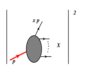
Figure 1: Parton distribution function.

The summation over $X$ reflects the inclusive nature of the description of the hadron structure by the parton distribution functions $f_{a/H}(x)$. The parton distribution functions $f_{a/H}(x)$ have been intensively studied in experiments on hard inclusive processes for the last 30 years. The classic process in this respect is the deep inelastic scattering (DIS) $eN\to e^{\prime}X$ whose structure functions are directly expressed in terms of $f_{a/H}(x)$.

The standard approach is to write the DIS structure function as the imaginary part of the virtual forward Compton amplitude $T_{\mu\nu}(q,p)$. In the most general nonforward case, the virtual Compton scattering amplitude is derived from the correlation function of two electromagnetic currents $J^{\mu}(x),J_{\nu}(y)$

$$T_{\mu\nu} = i\int d^{4}x\;\int d^{4}y\;e^{-i(qx)+i(q^{\prime}y)}\langle p^{\prime}|{\rm T}\left\{J_{\mu}(x)J_{\nu}(y)\right\}|p\rangle\ .$$ (1)

In the forward limit, the “final” photon has the momentum $q$ coinciding with that of the initial one. The momenta $p,p^{\prime}$ of the initial and “final” hadrons also coincide. The light-cone dominance of the virtual forward Compton amplitude is secured by high virtuality of the photons $-q^{2}\equiv Q^{2}>1$ GeV² and large total center-of-mass (cms) energy of the photon-hadron system $s=(p+q)^{2}$. The latter should be above resonance region, with the Bjorken ratio $x_{Bj}\equiv Q^{2}/2(pq)$ fixed.

An efficient way to study the behavior of Compton amplitudes in the Bjorken limit is to use the light–cone expansion for the product

$$\Pi_{\mu\nu}(x,y)\equiv i{\rm T}J_{\mu}(x)J_{\nu}(y)$$

of two vector currents in the coordinate representation. The leading order contribution is given by two “handbag” diagrams,

$$\Pi_{\mu\nu}(z\,|\,X)=\frac{z_{\rho}}{\pi^{2}z^{4}}\biggl{\{}s_{\mu\rho\nu\sigma}{\cal O}_{\sigma}(z\,|\,X)-i\epsilon_{\mu\rho\nu\sigma}{\cal O}_{5\sigma}(z\,|\,X)\biggl{\}}\ ,$$ (2)

where $s_{\mu\rho\nu\sigma}=g_{\mu\rho}g_{\nu\sigma}-g_{\mu\nu}g_{\rho\sigma}+g_{\mu\sigma}g_{\nu\rho}$,   $X=(x+y)/2$, $z=y-x$, and

$${\cal O}_{\sigma}(z\,|\,X) = \frac{1}{2}\,\left[\bar{\psi}(X-z/2)\gamma_{\sigma}\psi(X+z/2)\;-\;(z\rightarrow-z)\right]\ ,$$

$${\cal O}_{5\sigma}(z\,|\,X) = \frac{1}{2}\,\left[\bar{\psi}(X-z/2)\gamma_{\sigma}\gamma_{5}\psi(X+z/2)\;+\;(z\rightarrow-z)\right]\ .$$ (3)

Formally, the parton distribution functions provide parametrization of the forward matrix elements of quark and gluon operators on the light cone. For example, in the parton helicity averaged case (corresponding to the vector operator ${\cal O}_{\sigma}$) the $a$-quark/antiquark distributions are defined by

$$\langle p\,\,|\,\,\bar{\psi}_{a}(-z/2)\hat{z}E(0,z;A)\psi_{a}(z/2)\,\,|\,\,p\rangle\,$$

$$=\bar{u}(p)\hat{z}u(p)\int_{0}^{1}\,\left(e^{-ix(pz)}f_{a}(x)-e^{ix(pz)}f_{\bar{a}}(x)\right)\,dx\,+O(z^{2}),$$ (4)

where $E(0,z;A)$ is the standard path-ordered exponential (Wilson line) of the gluon field $A$ which secures gauge invariance of the nonlocal operator. In what follows, we will not write it explicitly. Throughout, we use the “Russian hat” notation $\hat{z}\equiv\gamma_{\mu}z^{\mu}$.

The non-leading (or higher-twist) $O(z^{2})$ terms in the above representation soften the light–cone singularity of the Compton amplitude, which results in suppression by powers of $1/Q^{2}$ (see Sec. 7 for a discussion of twist decomposition and higher–twist corrections).

The exponential factors $\exp[\mp ix(pz)]$ accompanying the quark and antiquark distributions reflect the fact that the field $\psi(z/2)$ appearing in the operator $\bar{\psi}(-z/2)\ldots\psi(z/2)$ consists of the quark annihilation operator (a quark with momentum $xp$ comes into this point) and the antiquark creation operator (i.e., an antiquark with momentum $xp$ goes out of this point). To get the relative signs with which quark and antiquark distributions appear in these definitions, we should take into account that antiquark creation and annihilation operators appear in $\bar{\psi}(-z/2)\ldots\psi(z/2)$ in opposite order.

In a similar way, one can introduce polarized quark densities $\Delta f_{a,\bar{a}}(x)$ which parametrize the forward matrix element of the axial operator $\bar{\psi}_{a}(-z/2)\hat{z}\gamma_{5}E(0,z;A)\psi_{a}(z/2)$.

Combining the parametrization (4) with the Compton amplitude (2) one obtains the QCD parton representation

$$T^{\mu\nu}(p,q)=\sum_{a}\int_{0}^{1}f_{a}(x)\,t^{\mu\nu}_{a}(xp,q)\,dx\biggl{\{}1+O(1/Q^{2})\biggr{\}}$$ (5)

for the hadron amplitude in terms of the perturbatively calculable hard parton amplitude $t^{\mu\nu}_{a}(xp,q)$ convoluted with the parton distribution functions $f_{a}(x)$ ($a=u,d,s,g,\ldots$) which describe/parametrize nonperturbative information about hadronic structure. The short-distance part of the handbag contribution is given by the hard quark propagator proportional to $1/[(xp+q)^{2}+i\epsilon]$. Its imaginary part contains the $\delta(-Q^{2}+2x(qp))$ factor (terms $O(p^{2})$ are neglected) which selects just the $x=x_{Bj}$ value from the $x$-integral. As a result, the DIS cross section is directly expressed in terms of $f_{a/H}(x_{Bj})$.

Figure 2: $a)$ General Compton amplitude; $b)$ $s$-channel handbag diagram; $c)$ $u$-channel handbag diagram.

Note, however, that the factorized representation is valid for the full Compton amplitude in which the parton densities are integrated over $x$. In other words, the variable $x$ in Eq.(5) has the meaning of the momentum fraction carried by the parton, but it is not equal to the Bjorken parameter $x_{Bj}$.

The basic parametrization (4) can be also written as an integral from $-1$ to 1 with a common exponential

$$\langle p\,\,|\,\,\bar{\psi}_{a}(-z/2)\hat{z}\psi_{a}(z/2)\,\,|\,\,p\rangle\,|\,=\bar{u}(p)\hat{z}u(p)\int_{-1}^{1}\,e^{-ix(pz)}\tilde{f}_{a}(x)\,dx\,+O(z^{2}).$$ (6)

For $x>0$, the distribution function $\tilde{f}_{a}(x)$ coincides with the quark distribution $f_{a}(x)$, while for $x<0$ it is given by (minus) the antiquark distribution $-f_{\bar{a}}(-x)$.

2.2 Distribution amplitudes

To give an example of another important type of nonperturbative functions describing hadronic structure, namely, the distribution amplitudes, let us consider the $\gamma^{*}\gamma\pi^{0}$ form factor. It is usually measured in $e^{+}e^{-}$ collisions, but for our purposes it is more convenient to represent it through the process in which electron is scattered with large momentum transfer $q$ off the pion target producing a real photon in the final state. The pion, in particular, can belong to the cloud surrounding a nucleon. In this case, the $\gamma^{*}\pi^{0}\to\gamma$ subprocess is a part of deeply virtual Compton scattering (DVCS) which will be considered in more detail later on.

The leading order contribution for large $Q^{2}$ is given by two handbag diagrams, and in the coordinate representation one deals with the same Compton amplitude (2). The only difference is that the nonlocal operators should be sandwiched between the one-pion state $|\,\pi(r)\,\rangle$ ($r$ is the pion momentum) and the vacuum $\langle\,0\,|$. Since the pion is a pseudoscalar particle, only the axial nonlocal operator ${\cal O}_{5\sigma}$ contributes, and the pion distribution amplitude $\varphi_{\pi}(\alpha)$ is the function parametrizing its matrix element

$$\langle 0\,\,|\,\,\bar{\psi}(-z/2)\hat{z}\gamma_{5}\psi(z/2)\,\,|\,\pi(r)\,\rangle\,\,=(rz)\int_{-1}^{1}\,e^{-i\alpha(rz)}\varphi_{\pi}(\alpha)d\alpha\,+O(z^{2}).$$ (7)

One can interpret $\varphi_{\pi}(\alpha)$ as the probability amplitude

$$\Psi\{\pi(r)\to q(yr)+\bar{q}((1-y)r)\}$$

to find the pion in a quark-antiquark state with the pion momentum $r$ shared in fractions $y\equiv(1+\alpha)/2$ and $1-y=(1-\alpha)/2$. Since the function $\varphi_{\pi}(\alpha)$ is even in $\alpha$, the use of the relative fraction $\alpha$ has some advantages when the symmetry properties are concerned.

Figure 3: Handbag diagrams and parton picture. $a)$ Virtual forward Compton amplitude expressed through the usual parton densities $f(x)$. $b)$ Form factor $\gamma^{*}\gamma\pi^{0}$ written in terms of the distribution amplitude $\varphi(\alpha)$.

3 Double distributions

3.1 DVCS and DDs

Now, let us consider deeply virtual Compton scattering (DVCS), an exclusive process $\gamma^{*}(q)N(p)\to\gamma(q^{\prime})N(p^{\prime})$ in which a highly virtual initial photon produces a real photon in the final state. The initial state of this reaction is in the Bjorken kinematics: $Q^{2}\equiv-q^{2}$ and $(pq)$ are large, while the ratio $x_{Bj}\equiv Q^{2}/2(pq)$ is fixed, just like in DIS. An extra variable is the momentum transfer $r\equiv p-p^{\prime}$. The simplest case is when $t\equiv r^{2}$ is small. This does not mean, of course, that the components of $r$ must be small: to convert a highly virtual photon into a real one, one needs $r$ with a large projection on $q$. Indeed, from $q^{\prime 2}=0$ it follows that

$$(q+r)^{2}=-Q^{2}+2(qr)+t=0,$$ (8)

i.e. $(qr)\approx-Q^{2}/2$ for small $t$. In the $t\to 0$ limit, we can write $(qr)=x_{Bj}(qp)$. Taking the initial momentum $p$ in the light cone “plus” direction and the momentum $q^{\prime}$ of the final photon in the light cone “minus” direction, we conclude that the momentum transfer $r$ in DVCS kinematics must have a non-zero plus component: $r^{+}=\zeta p^{+}$, with $\zeta=x_{Bj}$.

For large $Q^{2}$, the leading order contribution is given again by handbag diagrams. A new feature is that the nonperturbative part is described by nonforward matrix elements $\langle\,p-r\,|\ldots|\,p\,\rangle$ of ${\cal O}_{\sigma}$ and ${\cal O}_{5\sigma}$ operators. These matrix elements are parametrized by generalized parton distributions (GPDs). It is instructive to treat GPDs as kinematic “hybrids” of the usual parton densities $f(x)$ and distribution amplitudes $\varphi(\alpha)$. Indeed, $f(x)$ corresponds to the forward limit $r=0$, when the momentum $p$ flows only in the $s$-channel and the outgoing parton carries the momentum $xp^{+}$. On the other hand, if we take $p=0$, the momentum $r$ flows in the $t$-channel only and is shared in fractions $(1+\alpha)r^{+}/2$ and $(1-\alpha)r^{+}/2$. In general case, we deal with superposition of two momentum fluxes: the plus component $k^{+}$ of the parton momentum $k$ can be written as $xp^{+}+(1+\alpha)r^{+}/2$. To fully incorporate the symmetry properties of nonforward matrix elements, it is convenient to introduce the symmetric momentum variable $P=(p+p^{\prime})/2$ and write the parton momentum as

$$k^{+}=xP^{+}+(1+\alpha)r^{+}/2.$$ (9)

This decomposition corresponds to the following parametrization

$$\langle P-r/2|\bar{\psi}_{a}(-z/2)\hat{z}\psi_{a}(z/2)|P+r/2\rangle\,$$

$$=\bar{u}(p^{\prime})\hat{z}u(p)\,\int_{-1}^{1}\,dx\int_{-1+|x|}^{1-|x|}e^{-ix(Pz)-i\alpha(rz)/2}\,f_{a}(x,\alpha;t)\,d\alpha\,$$

$$+O(r)\,\,{\rm terms}\ +O(z^{2}),$$ (10)

where $f_{a}(x,\alpha;t)$ is the double distribution (DD).$\!{}^{{\bf?},{\bf?}}$ For the moment, we do not write explicitly “$O(r)$” terms corresponding to $\bar{u}(p^{\prime})\sigma_{\alpha\beta}r^{\alpha}z^{\beta}u(p)$ and $(rz)\bar{u}(p^{\prime})u(p)$ structures.

Figure 4: $a)$ Parton description of deeply virtual Compton scattering in terms of double distributions $f(x,\alpha;t)$. $b)$ Support region for $f(x,\alpha;t)$.

3.2 General properties of DDs

The support area for $f_{a}(x,\alpha;t)$ is shown on Fig. 4b. For any Feynman diagram, the spectral constraint $|x|+|\alpha|\leq 1$ can be proved in the $\alpha$-representation $\!{}^{{\bf?}}$ using the approach of Ref. 26. Comparing Eq. (4) with the $r=0$ limit of the DD definition (10) gives the “reduction formulas” relating the double distribution $f_{a}(x,\alpha;t=0)$ to the quark and antiquark parton densities

$$\int_{-1+x}^{1-x}\,f_{a}(x,\alpha;t=0)|_{x>0}\,d\alpha=f_{a}(x)$$ (11)

$$\int_{-1+|x|}^{1-|x|}\,f_{a}(x,\alpha;t=0)|_{x<0}\,d\alpha=-f_{\bar{a}}(-x)\,\,.$$ (12)

Hence, the positive-$x$ and negative-$x$ components of the double distribution $f_{a}(x,\alpha;t=0)$ can be treated as nonforward generalizations of quark and antiquark densities, respectively. The usual “forward” densities $f_{a}(x)$ and $f_{\bar{a}}(x)$ are thus given by integrating $f_{a}(x,\alpha\,;\,t=0)$ over vertical lines $x={\rm const}$ for $x>0$ and $x<0$, respectively. In principle, we cannot exclude the third possibility that the functions $f_{a}(x,\alpha;t)$ have singular terms at $x=0$ proportional to $\delta(x)$ or its derivative(s). Such terms have no projection onto the usual parton densities. We will denote them by $f_{M}(x,\alpha;t)$ $-$ they may be interpreted as coming from the $t$-channel meson-exchange type contributions. In this case, the partons just share the plus component of the momentum transfer $r$: information about the magnitude of the initial hadron momentum is lost if the exchanged particle can be described by a pole propagator $1/(t-m_{M}^{2})$. Hence, the meson-exchange contributions to a double distribution may look like

$$f_{M}^{+}(x,y;t)\sim\delta(x)\,\frac{\varphi_{M}^{+}(\alpha)}{m_{M}^{2}-t}\ \ \ {\rm or}\ \ \ f_{M}^{-}(x,\alpha;t)\sim\delta^{\prime}(x)\,\frac{\varphi^{-}_{M}(\alpha)}{m_{M}^{2}-t}\ \ ,\ \ {\rm etc.}\,,$$ (13)

where $\varphi_{M}^{\pm}(\alpha)$ are the functions related to the distribution amplitudes of the relevant mesons $M^{\pm}$. The two examples above correspond to $x$-even and $x$-odd parts of the double distribution $f(x,\alpha;t)$.

Due to hermiticity and time-reversal invariance properties of nonforward matrix elements, the DDs are even functions of $\alpha$,

$$\tilde{f}_{a}(x,\alpha;t)=\tilde{f}_{a}(x,-\alpha;t)\,.$$

In particular, the functions $\varphi_{M}^{\pm}(\alpha)$ for singular contributions $f_{M}^{\pm}(x,\alpha;t)$ are even functions $\varphi_{M}^{\pm}(\alpha)=\varphi_{M}^{\pm}(-\alpha)$ of $\alpha$ both for $x$-even and $x$-odd parts.

Note that the $\mu\leftrightarrow\nu$ symmetric part of the DVCS amplitude contains only the $C$-even operators ${\cal O}^{\sigma}_{a}$. Their matrix elements are parametrized

$$\langle\,p^{\prime},s^{\prime}\,|\,\,z^{\sigma}{\cal O}_{a}(-z/2,z/2)\,\,|\,\,p,s\rangle\,|\,_{z^{2}=0}$$

$$=\bar{u}(p^{\prime},s^{\prime})\hat{z}u(p,s)\,\int_{-1}^{1}dx\int_{-1+|x|}^{1-|x|}\,e^{-ix(Pz)-i\alpha(rz)/2}\,f_{a}^{S}(x,\alpha\,;\,t)\,d\alpha$$

$$+O(r)\,\,{\rm terms}$$ (14)

by the DDs

$$f_{a}^{S}(x,\alpha\,;\,t)\!=\!{\rm sign}(x)[f_{a}(|x|,\alpha\,;\,t)+f_{\bar{a}}(|x|,\alpha\,;\,t)]$$

which are odd functions of $x$. In applications to the hard meson electroproduction one also needs valence-type DDs

$$f_{a}^{V}(x,\alpha\,;\,t)\!=\![f_{a}(|x|,\alpha\,;\,t)-f_{\bar{a}}(|x|,\alpha\,;\,t)]$$

parametrizing matrix elements of $C$-odd operators $\bar{\psi}_{a}(-z/2)\hat{z}\psi_{a}(z/2)+\bar{\psi}_{a}(z/2)\hat{z}\psi_{a}(-z/2)$.

4 Skewed parton distributions

4.1 General definition

An important parameter for nonforward matrix elements is the coefficient of proportionality $\zeta=r^{+}/p^{+}$ (or $\xi=r^{+}/P^{+}$) between the plus components of the momentum transfer and the initial (or average) hadron momentum. It specifies the skewedness of the matrix elements. The two skewedness parameters are related by

$$\xi=\frac{\zeta}{2-\zeta}\ .$$ (15)

The characteristic feature implied by the definition of the double distribution (10) is the absence of the $\xi$-dependence in $f(x,\alpha;t)$. An alternative way to parametrize nonforward matrix elements of light-cone operators is to use $\xi$ and the total momentum fraction $\tilde{x}\equiv x+\xi\alpha$ as independent variables and introduce skewed parton distributions (SPDs). The shape of SPDs explicitly depends on the skewedness of the relevant nonforward matrix element.

There are two types of SPDs: off-forward parton distributions $\!{}^{{\bf?},{\bf?}}$ (OFPDs) $H(\tilde{x},\xi;t)$ and nonforward parton distributions $\!{}^{{\bf?},{\bf?}}$ (NFPDs) ${\cal F}_{\zeta}(X;t)$. The basic difference is that the skewedness parameter $\xi$ ($\zeta$) and the parton momentum $k^{+}$ in the OFPD (NFPD) formalism is measured in units of the average (initial) momentum $P^{+}$ ($p^{+}$). Hence, there are one-to-one relations between OFPDs and NFPDs.$\!{}^{{\bf?}}$ We start with OFPDs because they have simpler symmetry properties.

The relation between OFPDs $H(\tilde{x},\xi;t)$ and DDs $f(x,\alpha;t)$ is given just by the change of variables from $\{x,\alpha\}$ to $\{\tilde{x},\xi\}$,

$$H(\tilde{x},\xi;t)=\int_{-1}^{1}dx\int_{-1+|x|}^{1-|x|}\,\delta(x+\xi\alpha-\tilde{x})\,f(x,\alpha;t)\,d\alpha\,.$$ (16)

If we require that the light-cone plus components of both the momentum transfer $r$ and the final hadron momentum $p-r$ are positive (which is the case for DVCS), then $0\leq\zeta\leq 1$ and $0\leq\xi\leq 1$. Using the spectral property $0\leq|x|+|\alpha|\leq 1$ of double distributions we obtain that the OFPD variable $\tilde{x}$ satisfies the constraint $0\leq|\tilde{x}|\leq 1$. Note also that Eq. (16) formally allows to construct $\tilde{H}(\tilde{x},\xi;t)$ both for positive and negative values of $\xi$. Since the DDs $\tilde{f}(x,\alpha;t)$ are even functions of $\alpha$, the OFPDs $H(\tilde{x},\xi;t)$ are even functions of $\xi$:

$$\tilde{H}(\tilde{x},\xi;t)=\tilde{H}(\tilde{x},-\xi;t)\,.$$

This result was originally obtained by X. Ji $\!{}^{{\bf?}}$ who used hermiticity and time reversal invariance properties in the direct definition of OFPDs

$$\langle p^{\prime}|\bar{\psi}_{a}(-z/2)\hat{z}\psi_{a}(z/2)|p\rangle\,$$

$$=\bar{u}(p^{\prime})\hat{z}u(p)\int_{-1}^{1}\,e^{-i\tilde{x}(Pz)}\,H_{a}(\tilde{x},\xi;t)\,d\tilde{x}+O(r)\,\,{\rm term}\ +O(z^{2}).$$ (17)

Figure 5: Description of the nonforward matrix element in terms of $a)$ double distribution $f(x,\alpha;t)$ and $b)$ off-forward parton distribution $H(\tilde{x},\xi;t)$. $c)$ Integration lines for integrals relating OFPDs and DDs.

4.2 Structure of SPDs

The parton interpretation of the OFPD definition is the following: the quark going out of the parent hadron carries the fraction $\tilde{x}+\xi$ of the average hadron momentum $P^{+}$, while the momentum of the “returning” quark is $(\tilde{x}-\xi)P^{+}$. For definiteness, we shall assume below that $\xi$ is positive. Treating a quark with a negative momentum as an antiquark, we can distinguish 3 components of $H(\tilde{x},\xi;t)$. For $\tilde{x}>\xi$ both the initial fraction $\tilde{x}+\xi$ and the final one $\tilde{x}-\xi$ are positive. Hence, $H(\tilde{x},\xi;t)$ in this region corresponds to a modified quark distribution. Similarly, for $\tilde{x}<-\xi$ both fractions are negative, and $H(\tilde{x},\xi;t)$ can be treated as an antiquark distribution. In the third (middle) region, $-\xi<\tilde{x}<\xi$, the two fractions have opposite signs, and $H(\tilde{x},\xi;t)$ describes splitting of a quark-antiquark pair from the initial hadron. The total momentum carried by the $\bar{q}q$ pair is $2\xi P^{+}=r^{+}$, and it is shared in fractions $(\tilde{x}+\xi)P^{+}=(1+\beta)r^{+}/2$ and $(\xi-\tilde{x})P^{+}=(1-\beta)r^{+}/2$, where $\beta\equiv\tilde{x}/\xi$. Note that $|\beta|<1$ in the $|\tilde{x}|<\xi$ region. Hence, the third component can be interpreted as the probability amplitude for the initial hadron with momentum $(1+\xi)P^{+}$ to split into the final hadron with momentum $(1-\xi)P^{+}$ and a two-parton state with total momentum $r^{+}$ shared by the partons of the pair. Thus, we may expect that $H(\tilde{x},\xi;t)$ in the middle region looks more like a distribution amplitude.

The relation between DDs and SPDs can be illustrated on the DD support rhombus $|x|+|\alpha|\leq 1$ (see Fig. 5c). The delta-function in Eq. (16) specifies the line of integration in the $\{x,\alpha\}$ plane. To get $H(\tilde{x},\xi;t)$, one should integrate $f(x,\alpha)$ over $\alpha$ along a straight line $x=\tilde{x}-\xi\alpha$. Fixing some value of $\xi$, one deals with a set of parallel lines intersecting the $x$-axis at $x=\tilde{x}$. The upper limit of the $\alpha$-integration is determined by intersection of this line either with the line $x+\alpha=1$ (this happens if $\tilde{x}>\xi$) or with the line $-x+\alpha=1$ (if $\tilde{x}<\xi$). Similarly, the lower limit of the $\alpha$-integration is set by the line $x-\alpha=1$ for $\tilde{x}>-\xi$ or by the line $x+\alpha=-1$ for $\tilde{x}<-\xi$. The lines corresponding to $\tilde{x}=\pm\xi$ separate the rhombus into three parts generating the three components of $H(\tilde{x},\xi;t)$:

$$H_{a}(\tilde{x},\xi;t)=\theta(\xi\leq\tilde{x}\leq 1)\int_{-\frac{1-\tilde{x}}{1+\xi}}^{\frac{1-\tilde{x}}{1-\xi}}f_{a}(\tilde{x}-\xi\alpha,\alpha)\,d\alpha$$

$$+\theta(-\xi\leq\tilde{x}\leq\xi)\int_{-\frac{1-\tilde{x}}{1+\xi}}^{\frac{1+\tilde{x}}{1+\xi}}f_{a}(\tilde{x}-\xi\alpha,\alpha)\,d\alpha\,$$

$$+\theta(-1\leq\tilde{x}\leq-\xi)\int_{-\frac{1+\tilde{x}}{1-\xi}}^{\frac{1+\tilde{x}}{1+\xi}}f_{a}(\tilde{x}-\xi\alpha,\alpha)\,d\alpha.$$ (18)

Recall that integrating the DD $f(x,\alpha;t=0)$ over a vertical line gives the usual parton density $f(x)$. To get the $t=0$ SPDs one should scan the same DD along the lines having a $\xi$-dependent slope. Thus, one can try to build models for SPDs using information about usual parton densities. Note, however, that the usual parton densities are insensitive to the meson-exchange type contributions $H_{M}(\tilde{x},\xi;t)$ coming from the singular $x=0$ parts of DDs. Thus, information contained in SPDs originates from two physically different sources: meson-exchange type contributions $H_{M}(\tilde{x},\xi;t)$ and the functions $H_{M}(\tilde{x},\xi;t)$ obtained by scanning the $x\neq 0$ parts of DDs $f(x,\alpha;t)$. The support of exchange contributions is restricted to $|\tilde{x}|\leq\xi$. Up to rescaling, the function $H_{M}(\tilde{x},\xi;t)$ has the same shape for all $\xi$, e.g., $\varphi_{M}(\tilde{x}/\xi;t)/|\xi|$. For any nonvanishing $\xi$, these exchange terms become invisible in the forward limit $\xi\to 0$. On the other hand, interplay between $\tilde{x}$ and $\xi$ dependences of the component resulting from integrating the $x\neq 0$ part of DDs is quite nontrivial. Its support in general covers the whole $-1\leq\tilde{x}\leq 1$ region for all $\xi$ including the forward limit $\xi$ in which they convert into the usual (forward) densities $f^{a}(x)$, $f^{\bar{a}}(x)$. The latter are rather well known from inclusive measurements. at small $t$.

4.3 Polynomiality and analyticity

In our derivation, DDs are the starting point, while SPDs are derived from them by integration. However, even if one starts directly with SPDs, the latter possess a property which can be incorporated only within the formalism of double distributions. Namely, the $\tilde{x}^{N}$ moment of $H(\tilde{x},\xi;t)$ must be an $N$th order polynomial of $\xi$. This restriction on the interplay between $\tilde{x}$ and $\xi$ dependences of $H(\tilde{x},\xi;t)$ follows $\!{}^{{\bf?}}$ from the simple fact that the Lorentz indices $\mu_{1}\ldots\mu_{N}$ of the nonforward matrix element of a local operator $O^{\mu_{1}\ldots\mu_{N}}$ can be carried either by $P^{\mu_{i}}$ or by $r^{\mu_{i}}$. As a result,

$$\langle P-r/2|\phi(0)(\stackrel{{\scriptstyle\leftrightarrow}}{{\partial^{+}}})^{N}\phi(0)|P+r/2\rangle=\sum_{k=0}^{N}{N\choose k}(P^{+})^{N-k}(r^{+})^{k}A_{Nk}\,$$

$$=(P^{+})^{N}\sum_{k=0}^{N}{N\choose k}\xi^{k}A_{Nk}\,,$$ (19)

where ${N\choose k}\equiv N!/(N-k)!k!$ is the combinatorial coefficient. Our derivation (16) of OFPDs from DDs automatically satisfies the polynomiality condition (19), since

$$\int_{-1}^{1}H(\tilde{x},\xi;t)\,\tilde{x}^{N}\,d\tilde{x}=\sum_{k=0}^{N}\,\xi^{k}\,{N\choose k}\,\int_{-1}^{1}dx\int_{-1+|x|}^{1-|x|}\tilde{f}(x,\alpha)\,x^{N-k}\alpha^{k}\,d\alpha\ .$$ (20)

Hence, the coefficients $A_{Nk}$ in (19) are given by double moments of DDs. This means that modeling SPDs one cannot choose the coefficients $A_{Nk}$ arbitrarily: symmetry and support properties of DDs dictate a nontrivial interplay between $N$ and $k$ dependences of $A_{Nk}$’s. After this observation, the use of DDs is a necessary step in building consistent parametrizations of SPDs.

The formalism of DDs also allows one to easily establish some important properties of skewed distributions. Notice that due to the cusp at the upper corner of the DD support rhombus, the length of the integration line nonanalytically depends on $\tilde{x}$ for $\tilde{x}=\pm\xi$. Hence, unless a double distribution identically vanishes in a finite region around the upper corner of the DD support rhombus, the $\tilde{x}$-dependence of the relevant nonforward distribution must be nonanalytic at the border points $\tilde{x}=\pm\xi$. Still, the length of the integration line is a continuous function of $\tilde{x}$. As a result, if the double distribution $f(x,\alpha;t)$ is not too singular for small $x$, the skewed distribution $H(\tilde{x},\xi;t)$ is continuous at the nonanalyticity points $\tilde{x}=\pm\xi$. Because of the $1/(\tilde{x}\pm\xi)$ factors contained in hard amplitudes, this property is crucial for PQCD factorization in DVCS and other hard electroproduction processes.

Note, that there may be also the exchange contributions $H_{M}(\tilde{x},\xi;t)$. If it comes from a $\delta(x)\varphi(\alpha)$ type term and $\varphi(\alpha)$ vanishes at the end-points $\alpha=\pm 1$, the $H_{M}(\tilde{x},\xi;t)$ part of SPD vanishes at $\tilde{x}=\pm\xi$. The total function $H(\tilde{x},\xi;t)$ is then continuous at the nonanalyticity points $x=\pm\,\xi$. In the $C$-even case, the DDs should be odd in $x$, hence the singular term involves $\delta^{\prime}(x)\varphi(\alpha)$ (or even higher odd derivatives of $\delta(x)$). One can get a continuous SPD in this case only if $\varphi^{\prime}(\alpha)$ vanishes at the end points.

4.4 Nonforward parton distribution functions

In the NFPD formalism,$\!{}^{{\bf?}}$ the skewedness parameter $\zeta\equiv r^{+}/p^{+}$ and the parton momentum $k^{+}$ are measured in units of the initial momentum $p^{+}$. Again, one can start with double distributions $F(x,y;t)$ writing the outgoing parton momentum as $k^{+}=xp^{+}+yr^{+}$ and that of the returning one as $xp^{+}-(1-y)r^{+}$ (see Fig. 6a). The support area for $F(x,y;t)$ is specified by $-1\leq x\leq 1$, $0\leq y\leq 1$, $0\leq x+y\leq 1$ (see Fig. 6c). The relation between $F_{a}(x,y;t=0)$ and the usual quark and antiquark densities is given by the “reduction formulas”

$$\int_{0}^{1-x}\,F_{a}(x,y;t=0)|_{x>0}\,dy=f_{a}(x)\ ;\ \int_{-x}^{1}\,F_{a}(x,y;t=0)|_{x<0}\,dy=-f_{\bar{a}}(-x)\,\,.$$ (21)

If we define the “tilded” DDs by

$$\tilde{F}_{a}(x,y;t)=F_{a}(x,y;t)_{x>0}\ ;\ \tilde{F}_{\bar{a}}(x,y;t)=-F_{a}(-x,1-y;t)_{x<0}\,,$$

then $x$ is always positive and the reduction formulas

$$\int_{0}^{1-x}\,\tilde{F}_{a,\bar{a}}(x,y;t=0)|_{x\neq 0}\,dy=f_{a,\bar{a}}(x)$$ (22)

have the same form in both cases. The new antiquark DDs $\tilde{F}_{\bar{a}}(x,y;t)$ also “live” on the triangle $0\leq x,y,x+y\leq 1$.

Figure 6: Description of nonforward matrix elements in terms of $a)$ double distributions $F(x,y;t)$ and $b)$ nonforward parton distributions ${\cal F}_{\zeta}^{i}(X;t)$. $c)$ Integration lines for the integrals relating NFPDs and DDs.

The $\alpha\to-\alpha$ symmetry of the OFPD-oriented DDs $f(x,\alpha;t)$ corresponds to the symmetry of $\tilde{F}_{a,\bar{a}}(x,y;t)$ with respect to the interchange $y\leftrightarrow 1-x-y$ (“Munich symmetry”) established in Ref. 27.

Using $r^{+}=\zeta p^{+}$ and introducing the total momentum fraction $X\equiv x+\zeta y$, we define the nonforward parton distributions (see Fig. 6b)

$${\cal F}_{\zeta}^{i}(X;t)=\int_{0}^{1}dx\int_{0}^{1-x}\,\delta(x+\zeta y-X)\,\tilde{F}_{i}(x,y;t)\,dy\ .$$ (23)

The relation between NFPDs and DDs $\tilde{F}_{i}(x,y)$ can be illustrated on the DD support triangle $0\leq x,y,x+y\leq 1$ (see Fig. 6c). To get ${\cal F}_{\zeta}(X;t)$, one should integrate $\tilde{F}(x,y;t)$ over $y$ along a straight line $x=X-\zeta y$. The upper limit of the $y$-integration is determined by intersection of this line either with the line $x+y=1$ (this happens if $X>\zeta$) or with the $y$-axis (if $X<\zeta$):

$${\cal F}_{\zeta}^{i}(X;t) = \theta(X>\zeta)\int_{0}^{(1-X)/(1-\zeta)}\,\,\tilde{F}_{i}(X-\zeta y,y;t)\,dy\$$ (24)

$$+ \theta(X<\zeta)\int_{0}^{X/\zeta}\,\,\tilde{F}_{i}(X-\zeta y,y;t)\,dy.$$

The returning parton carries the fraction $X-\zeta$ of the initial hadron momentum $p^{+}$, which is positive in the $X>\zeta$ region (where NFPDs can be treated as modified parton densities) and negative in the $X<\zeta$ region (where NFPDs resemble distribution amplitudes).

For reference purposes, we present the relations between the NFPD and OFPD variables

$$\zeta=\frac{2\xi}{1+\xi},\ \ \ X=\frac{\tilde{x}+\xi}{1+\xi},\ \ \ X^{\prime}\equiv X-\zeta=\frac{\tilde{x}-\xi}{1+\xi},\ \ \ \tilde{x}=\frac{X-\zeta/2}{1-\zeta/2}\ .$$ (25)

4.5 Relation to form factors

GPDs depend on the invariant momentum transfer $t$, hence, they may also be treated as generalizations of hadronic form factors. In particular, $H_{a}(\tilde{x},\xi;t)$ is related to the Dirac form factor of the proton,$\!{}^{{\bf?}}$

$$\sum_{a}e_{a}\int_{-1}^{1}H_{a}(x,\xi,t)\,dx=F_{1}(t)\,,$$ (26)

where $e_{a}$ is the electric charge of the relevant quark. Just like for form factors, there are extra generalized parton distributions $\!{}^{{\bf?}}$ $E_{a}(x,\xi,t)$ corresponding to helicity flip in the nonforward matrix element. They are related to $F_{2}(t)$ form factor,

$$\sum_{a}e_{a}\int_{-1}^{1}E_{a}(x,\xi,t)\,dx=F_{2}(t)\,.$$ (27)

Note that though the shape of GPDs changes when $\xi$ is varied, the integrals (26), (27) do not depend on $\xi$. Since the $E$ functions are accompanied by the $r_{\mu}$ factor in the parametrization of the nonforward matrix element

$$\langle p^{\prime}|\bar{\psi}\gamma_{\mu}\psi|p\rangle\sim\bar{u}(p^{\prime})\gamma_{\mu}u(p)``H"+\frac{1}{2M}\bar{u}(p^{\prime})\sigma_{\mu\nu}r^{\nu}u(p)``E"\ ,$$

they are invisible in deep inelastic scattering described by exactly forward $r=0$ Compton amplitude. However, the $t=0,\xi=0$ limit of the $E$ distributions exists,

$$E_{a}(x,\xi=0;t=0)\equiv e_{a}(x)\ .$$

In particular, for $t=0$ the integral (27) gives the anomalous magnetic moment. Moreover, the recent interest to DVCS and generalized parton distributions is largely due to observation made by X. Ji $\!{}^{{\bf?}}$ that the integral

$$J_{q}=\frac{1}{2}\sum_{a}\int_{-1}^{1}\left[f_{a}(x)+e_{a}(x)\right]\,xdx\,$$ (28)

is related to the total spin and orbital momentum contribution of the quarks into the proton spin. Ji proposed to use deeply virtual Compton scattering to get access to the $e_{a}(x)$ functions. These function can be also accessed in hard meson electroproduction processes.$\!{}^{{\bf?}}$

The DVCS amplitude contains two other generalized parton distributions $\tilde{H}(x,\xi;t)$ and $\tilde{E}(x,\xi;t)$. They parametrize the nonforward matrix element of the axial operator $\!{}^{{\bf?}}$

$$\langle p^{\prime}|\bar{\psi}\gamma_{\mu}\gamma_{5}\psi|p\rangle\sim\bar{u}(p^{\prime})\gamma_{\mu}u(p)``\tilde{H}"+\frac{r_{\mu}}{2M}\bar{u}(p^{\prime})u(p)``\tilde{E}"\ .$$ (29)

In the forward limit, the $\tilde{H}$-distributions reduce to the polarized parton densities $\tilde{H}_{a}(x,\xi=0;t=0)=\Delta f_{a}(x)$. After the $x$-integration, the $\tilde{H}_{a}(x,\xi=0;t=0)$ distributions produce the flavor components of the axial form factor $G_{A}(t)$. Similarly, the functions $\tilde{E}(x,\xi;t)$ are related to the pseudoscalar form factor $G_{P}(t)$. At small $t$, they are dominated by the pion pole term $1/(t-m_{\pi}^{2})$.

4.6 Gluon distributions

In a similar way, we can write parametrizations defining double and skewed distributions for gluonic operators

$$\langle P-r/2\,|\,z_{\mu}z_{\nu}G_{\mu\alpha}^{a}(-z/2)E_{ab}(-z/2,z/2;A)G_{\alpha\nu}^{b}(z/2)\,|\,P+r/2\rangle\,$$

$$=(Pz)\bar{u}(p^{\prime})\hat{z}u(p)\,\int_{-1}^{1}\,dx\int_{-1+|x|}^{1-|x|}e^{-ix(Pz)-i\alpha(rz)/2}\,xf_{g}(x,\alpha;t)\,d\alpha\,+\ldots$$

$$=(Pz)\bar{u}(p^{\prime})\hat{z}u(p)\,\int_{-1}^{1}e^{-i\tilde{x}(Pz)}\,H_{g}(\tilde{x},\xi;t)\,d\tilde{x}+\ldots\ .$$ (30)

Note, that the gluon SPD $H_{g}(\tilde{x},\xi;t)$ is constructed from $xf_{g}(x,\alpha;t)$. Just like the singlet quark distribution, the gluon double distribution $f_{g}(x,\alpha;t)$ is an odd function of $x$.

5 Modeling GPDs

There are two approaches used to model GPDs. One is based on a direct calculation of parton distributions in specific dynamical models, such as bag model,$\!{}^{{\bf?}}$ chiral soliton model,$\!{}^{{\bf?}}$ light-cone formalism,$\!{}^{{\bf?}}$ etc. Another approach $\!{}^{{\bf?},{\bf?},{\bf?}}$ is a phenomenological construction based on reduction formulas relating GPDs to usual parton densities $f(x),\Delta f(x)$ and form factors $F_{1}(t),F_{2}(t),G_{A}(t),G_{P}(t)$. The most convenient way to construct such models is to start with double distributions $f(x,\alpha;t)$.

5.1 Modeling DDs

Let us consider the limiting case $t=0$. Our interpretation of the $x$-variable as the fraction of the $P$ momentum and the reduction formula stating that the integral of $f_{a}(x,\alpha)$ over $\alpha$ gives the usual parton density $f_{a}(x)$ suggest that the profile of $f_{a}(x,\alpha)$ in the $x$-direction follows the shape of $f_{a}(x)$. Thus, it make sense to write

$$f(x,\alpha)=h(x,\alpha)\,f(x)\,,$$ (31)

where the function $h(x,\alpha)$ normalized by

$$\int_{-1+|x|}^{1-|x|}h(x,\alpha)\,d\alpha\,=1$$ (32)

characterizes the profile of $f(x,\alpha)$ in the $\alpha$-direction. The profile function should be symmetric with respect to $\alpha\to-\alpha$ because DDs $\tilde{f}(x,\alpha)$ are even in $\alpha$. For a fixed $x$, the function $h(x,\alpha)$ describes how the longitudinal momentum transfer $r^{+}$ is shared between the two partons. Hence, the shape of $h(x,\alpha)$ should look like a symmetric meson distribution amplitude $\varphi(\alpha)$. Recalling that DDs have the support restricted by $|\alpha|\leq 1-|x|$, to get a more complete analogy with DAs, it makes sense to rescale $\alpha$ as $\alpha=(1-|x|)\beta$ introducing the variable $\beta$ with $x$-independent limits: $-1\leq\beta\leq 1$. The simplest model is to assume that the $\beta$–profile is a universal function $g(\beta)$ for all $x$. Possible simple choices for $g(\beta)$ may be $\delta(\beta)$ (no spread in $\beta$-direction), $\frac{3}{4}(1-\beta^{2})$ (characteristic shape for asymptotic limit of nonsinglet quark distribution amplitudes), $\frac{15}{16}(1-\beta^{2})^{2}$ (asymptotic shape of gluon distribution amplitudes), etc. In the variables $x,\alpha$, this gives

$$h^{(\infty)}(x,\alpha)=\delta(\alpha)\,\ ,\ h^{(1)}(x,\alpha)=\frac{3}{4}\frac{(1-|x|)^{2}-\alpha^{2}}{(1-|x|)^{3}}\,,$$

$$h^{(2)}(x,\alpha)=\frac{15}{16}\frac{[(1-|x|)^{2}-\alpha^{2}]^{2}}{(1-|x|)^{5}}\,\ .$$ (33)

These models can be treated as specific cases of the general profile function

$$h^{(b)}(x,\alpha)=\frac{\Gamma(2b+2)}{2^{2b+1}\Gamma^{2}(b+1)}\frac{[(1-|x|)^{2}-\alpha^{2}]^{b}}{(1-|x|)^{2b+1}}\,,$$ (34)

whose width is governed by the parameter $b$.

5.2 Modeling SPDs

Let us analyze the structure of SPDs obtained from these simple models. In particular, taking $f^{(\infty)}(x,\alpha)=\delta(\alpha)f(x)$ gives the simplest model $H^{(\infty)}(\tilde{x},\xi;t=0)=f(x)$ in which OFPDs at $t=0$ have no $\xi$-dependence. For DDs producing nonforward parton distributions ${\cal F}_{\zeta}(X;t=0)$, this is equivalent to the $F^{(\infty)}(x,y)=\delta(y-\bar{x}/2)f(x)$ model, which gives

$${\cal F}_{\zeta}^{(\infty)}(X)=\frac{\theta(X\geq\zeta/2)}{1-\zeta/2}f\left(\frac{X-\zeta/2}{1-\zeta/2}\right)\,,$$ (35)

i.e., NFPDs for non-zero $\zeta$ are obtained from the forward distribution $f(X)\equiv{\cal F}_{\zeta=0}(X)$ by shift and rescaling.

In case of the $b=1$ and $b=2$ models, simple analytic results can be obtained only for some explicit forms of $f(x)$. For the “valence quark”-oriented ansatz $\tilde{f}^{(1)}(x,\alpha)$, the following choice of a normalized distribution

$$f^{(1)}(x)=\frac{\Gamma(5-a)}{6\,\Gamma(1-a)}\,x^{-a}(1-x)^{3}$$ (36)

is both close to phenomenological quark distributions and produces a simple expression for the double distribution since the denominator $(1-x)^{3}$ factor in Eq. (33) is canceled. As a result, the integral in Eq. (18) is easily performed and we get

$$\tilde{H}^{1}_{V}(\tilde{x},\xi)|_{|\tilde{x}|\geq\xi} = \frac{1}{\xi^{3}}\left(1-\frac{a}{4}\right)\left\{\left[(2-a)\xi(1-\tilde{x})(x_{+}^{2-a}+x_{-}^{2-a})\right.\right.$$ (37)

$$+ \left.\left.(\xi^{2}-\tilde{x})(x_{+}^{2-a}-x_{-}^{2-a})\right]\,\theta(\tilde{x})+(\tilde{x}\to-\tilde{x})\right\}$$

for $|\tilde{x}|\geq\xi$ and

$$\tilde{H}^{1}_{V}(\tilde{x},\xi)|_{|\tilde{x}|\leq\xi}=\frac{1}{\xi^{3}}\left(1-\frac{a}{4}\right)\left\{x_{+}^{2-a}[(2-a)\xi(1-\tilde{x})+(\xi^{2}-x)]+(\tilde{x}\to-\tilde{x})\right\}$$ (38)

in the middle $-\xi\leq\tilde{x}\leq\xi$ region. We use here the notation $x_{+}=(\tilde{x}+\xi)/(1+\xi)$ and $x_{-}=(\tilde{x}-\xi)/(1-\xi)$. To extend these expressions onto negative values of $\xi$, one should substitute $\xi$ by $|\xi|$. One can check, however, that no odd powers of $|\xi|$ would appear in the $\tilde{x}^{N}$ moments of $\tilde{H}^{1V}(\tilde{x},\xi)$. Furthermore, these expressions are explicitly non-analytic for $x=\pm\xi$. This is true even if $a$ is integer. Discontinuity at $x=\pm\xi$, however, appears only in the second derivative of $\tilde{H}^{1V}(\tilde{x},\xi)$, i.e., the model curves for $\tilde{H}^{1V}(\tilde{x},\xi)$ look very smooth (see Fig. 7, where the curves for NFPDs are also shown).

Figure 7: Valence quark distributions: NFPDs $F^{q}_{\zeta}(X)$ (left) and OFPDs $\tilde{H}^{1}_{V}(\tilde{x},\xi)$ (right) with $a=0.5$ for several values of $\zeta$, namely, 0.1, 0.2, 0.4, 0.6, 0.8 and corresponding values of $\xi=\zeta/(2-\zeta)$. Lower curves correspond to larger values of $\zeta$.

For $a=0$, the $x>\xi$ part of OFPD has the same $x$-dependence as its forward limit, differing from it by an overall $\xi$-dependent factor only,

$$\tilde{H}^{1V}(\tilde{x},\xi)|_{a=0}=4\,\frac{(1-|\tilde{x}|)^{3}}{(1-\xi^{2})^{2}}\,\theta(|\tilde{x}|\geq\xi)\,+2\,\frac{\xi+2-3\tilde{x}^{2}/\xi}{(1+\xi)^{2}}\,\theta(|\tilde{x}|\leq\xi)\,.$$ (39)

The $(1-|\tilde{x}|)^{3}$ behavior can be trivially continued into the $|\tilde{x}|<\xi$ region. However, the actual behavior of $\tilde{H}^{1V}(\tilde{x},\xi)|_{a=0}$ in this region is given by a different function. In other words, $\tilde{H}^{1V}(\tilde{x},\xi)|_{a=0}$ can be represented as a sum of a function analytic at border points and a contribution whose support is restricted by $|\tilde{x}|<\xi$. It should be emphasized that despite its DA-like appearance, this contribution should not be treated as an exchange-type term. It is generated by the regular $x\neq 0$ part of the DD, and, unlike the $\varphi(\tilde{x}/\xi)/\xi$ functions its shape changes with $\xi$, the function becoming very small for small $\xi$.

Figure 8: Model for singlet quark distributions: OFPDs $H^{1}_{S}(\tilde{x},\xi)$ for values of $\xi$ corresponding to $\zeta$ equal to 0.2, 0.4, 0.6. Lower curves correspond to larger values of $\zeta$.

For the singlet quark distribution, the DDs $\tilde{f}^{S}(x,\alpha)$ should be odd functions of $x$. Still, we can use the model like (36) for the $x>0$ part, but take $\tilde{f}^{S}(x,\alpha)|_{x\neq 0}=A\,f^{(1)}(|x|,\alpha)\,{\rm sign}(x)$. Note, that the integral (18) producing $\tilde{H}^{S}(\tilde{x},\xi)$ in the $|\tilde{x}|\leq\xi$ region would diverge for $\alpha\to\tilde{x}/\xi$ if $a\geq 1$, which is the usual case for standard parametrizations of singlet quark distributions for sufficiently large $Q^{2}$. However, due to the antisymmetry of $\tilde{f}^{S}(x,\alpha)$ with respect to $x\to-x$ and its symmetry with respect to $\alpha\to-\alpha$, the singularity at $\alpha=\tilde{x}/\xi$ can be integrated using the principal value prescription which in this case produces the $x\to-x$ antisymmetric version of Eqs. (37) and (38). For $a=0$, its middle part reduces to

$$\tilde{H}^{1S}(\tilde{x},\xi)|_{|\tilde{x}|\leq\xi,a=0}=2x\,\frac{3\xi^{2}-2x^{2}\xi-x^{2}}{\xi^{3}(1+\xi)^{2}}\,.$$ (40)

The shape of singlet SPDs in this model is shown in Fig. 8

5.3 Polyakov-Weiss terms

Note, that the operator $\bar{\psi}(-z/2)\hat{z}\psi(z/2)$ is proportional to $z$. Hence, parametrizing its matrix elements in terms of parton distributions, it makes sense to use the structures which are also linear in $z$, like $\bar{u}(p^{\prime})\hat{z}u(p)$, $\bar{u}(p^{\prime})(\hat{z}\hat{r}-\hat{r}\hat{z})u(p)$ for the nucleon target, $(Pz)$ for the pion target, etc. However, there is a subtlety emphasized by Polyakov and Weiss.$\!{}^{{\bf?}}$ Namely, using parametrization by DDs, one treats $(Pz)$ and $(rz)$ as independent variables. This means that in the pion case, e.g., one should deal both with $(Pz)$ and $(rz)$ structures:

$$\langle P-r/2\,|\,\bar{\psi}(-z/2)\hat{z}\psi(z/2)\,|\,P+r/2\rangle$$

$$=2(Pz)\int_{-1}^{1}\,dx\int_{-1+|x|}^{1-|x|}e^{-ix(Pz)-i\alpha(rz)/2}\,f(x,\alpha;t)\,d\alpha\,$$

$$+(rz)\int_{-1}^{1}e^{-i\alpha(rz)/2}D(\alpha;t)\,d\alpha\ ,$$ (41)

where the Polyakov-Weiss (PW) $\!{}^{{\bf?}}$ term $D(\alpha;t)$ accumulates the $r^{\mu_{1}}\ldots r^{\mu_{n}}$ parts of the expansion for the matrix elements of the local operators $\bar{\psi}(0)\gamma^{\mu_{1}}D^{\mu_{2}}\ldots D^{\mu_{n}}\psi(0)$. There is no sensitivity in the $D$-term contribution to the value of the average momentum $P$ term: the parton momenta depend only on $r$. Hence, the $D$-term is a particular case of the exchange contributions.

Switching to skewed parton distributions, one deals with just one structure $(Pz)$, and one can incorporate the PW term contribution $\!{}^{{\bf?}}$ $D(\tilde{x}/\xi;t)\theta(|\tilde{x}|<\xi)$ into $H(\tilde{x},\xi;t)$.

In the nucleon case,$\!{}^{{\bf?}}$ the additional structure is $(rz)\bar{u}(p^{\prime})u(p)$. As a result, the skewed distributions $H,E$ have two components, one is obtained from the relevant DD and another comes from the $D$-term

$$H(\tilde{x},\xi;t)=H_{DD}(\tilde{x},\xi;t)+D(\tilde{x}/\xi;t)\theta(|\tilde{x}|<\xi)\,,$$ (42)

$$E(\tilde{x},\xi;t)=E_{DD}(\tilde{x},\xi;t)-D(\tilde{x}/\xi;t)\theta(|\tilde{x}|<\xi)\ .$$ (43)

Note, that the $D$-term drops from the Ji’s sum rule,$\!{}^{{\bf?},{\bf?}}$ since $H+E=H_{DD}+E_{DD}$.

It should be noted that explicit calculations of skewed parton distributions performed within the chiral soliton model $\!{}^{{\bf?}}$ show that the middle region behavior of SPDs strongly resembles that of distribution amplitudes.

5.4 Inequalities

In the case when $\tilde{x}>\xi$, the integration line producing $H(\tilde{x},\xi;t)$ (see Fig. 5c) is inside the space between two vertical lines giving the usual parton densities $f(x_{-})$ and $f(x_{+})$, with $x_{+}=(\tilde{x}+\xi)/(1+\xi)$ and $x_{-}=(\tilde{x}-\xi)/(1-\xi)$:

$$H_{a}(\tilde{x},\xi;t)=\theta(\xi\leq\tilde{x}\leq 1)\int_{x_{-}}^{x_{+}}f_{a}(x,(\tilde{x}-x)/\xi)\,\frac{dx}{\xi}dx+\ldots\ \ .$$ (44)

The combinations $x_{-},x_{+}$ have a very simple interpretation: they measure the momentum of the initial or final parton in units of the momentum of the relevant hadron. Assuming a monotonic decrease of the double distribution $f(x,\alpha)$ in the $x$-direction and a universal profile in the $\alpha$-direction, one may expect that $H_{a}(\tilde{x},\xi;t)$ is larger than $f(x_{+})$ but smaller than $f(x_{-})$. Inequalities between forward and nonforward distributions were discussed in Refs. 31, 19, 32. They are based on the application of the Cauchy-Schwartz inequality

$$|\langle N[(1-\xi)P];(\tilde{x}-\xi)P;S|\,N[(1+\xi)P];(\tilde{x}+\xi)P;S\rangle|^{2}$$

$$\leq\sum_{S}\langle N[(1+\xi)P];(\tilde{x}+\xi)P;S|\,N[(1+\xi)P];(\tilde{x}+\xi)P;S\rangle$$

$$\times\sum_{S^{\prime}}\langle N[(1-\xi)P];(\tilde{x}-\xi)P;S^{\prime}|\,N[(1-\xi)P];(\tilde{x}-\xi)P;S^{\prime}\rangle$$ (45)

to the skewed parton distributions written generically as

$$H(\tilde{x},\xi;t)=\sum_{S}\langle N[(1-\xi)P];(\tilde{x}-\xi)P;S|\,N[(1+\xi)P];(\tilde{x}+\xi)P;S\rangle\ ,$$ (46)

where $|N[(1\pm\xi)P];(\tilde{x}\pm\xi)P;S\rangle$ describes the probability amplitude that the nucleon with momentum $(1\pm\xi)P$ converts into a parton with momentum $(\tilde{x}\pm\xi)P$ and spectators $S$. The forward matrix elements give the usual parton densities

$$\sum_{S}\langle N[(1\pm\xi)P];(\tilde{x}\pm\xi)P;S\rangle\,=\frac{1}{1\pm\xi}\,f(x_{\pm}).$$ (47)

As a result, one obtains $\!{}^{{\bf?},{\bf?},{\bf?}}$ for the quark distributions

$$H_{a}(\tilde{x},\xi;t)\leq\sqrt{\frac{f_{a}(x_{+})f_{a}(x_{-})}{1-\xi^{2}}}\,.$$ (48)

For the gluon distribution, one has

$$H_{g}(\tilde{x},\xi;t)\leq\sqrt{x_{+}x_{-}{f_{g}(x_{+})f_{g}(x_{-})}}\,.$$ (49)

It is clear that the whole consideration makes sense only if $\tilde{x}>\xi$. If $\tilde{x}<\xi$, the integration line $x=\tilde{x}-\xi\alpha$ intersects the line $x=0$, where the usual parton densities are infinite. Furthermore, when negative $x$ are involved, the behavior of DDs along the line cannot be monotonic. Another deficiency of the Cauchy-Schwartz-type inequalities is that they do not give the lower bound for nonforward distributions though our graphical interpretation suggests that $H(\tilde{x},\xi;t=0)$ is larger than $f(x_{+})$ if the $x$-dependence of the double distribution $f(x,\alpha)$ along the lines $\alpha=k(1-|x|)$ is monotonic.

5.5 SPDs at small skewedness

To study the deviation of skewed distributions from their forward counterparts for small $\xi$ (or $\zeta$), let us consider the $x\geq\xi$ part of $H(x,\xi)$ (see Eq. (18)) and use its expansion in powers of $\xi$

$$H(\tilde{x};\xi)|_{\tilde{x}\geq\xi} = f(\tilde{x})+\xi^{2}\left[\frac{1}{2}\int_{-(1-\tilde{x})}^{(1-\tilde{x})}\frac{\partial^{2}f(\tilde{x},\alpha)}{\partial\tilde{x}^{2}}\,\alpha^{2}\,d\alpha\right.$$ (50)

$$+ \left.(1-\tilde{x})^{2}\left.\left(\frac{\partial f(\tilde{x},\alpha)}{\partial\alpha}-2\frac{\partial f(\tilde{x},\alpha)}{\partial\tilde{x}}\right)\right|_{\alpha=1-\tilde{x}}\right]+\ldots\,.$$

where $f(\tilde{x})$ is the forward distribution. For small $\xi$, the corrections are formally $O(\xi^{2})$. However, if $f(x,\alpha)$ has a singular behavior like $x^{-a}$, then

$$\frac{\partial^{2}f(\tilde{x},\alpha)}{\partial\tilde{x}^{2}}\sim\frac{a(1+a)}{\tilde{x}^{2}}f(\tilde{x},\alpha)\ ,$$

and the relative suppression of the first correction is $O(\xi^{2}/\tilde{x}^{2})$. Though the corrections are tiny for $\tilde{x}\gg\xi$, in the region $\tilde{x}\sim\xi$ they have no parameter smallness. It is easy to write explicitly all the terms which are not suppressed in the $\tilde{x}\sim\xi\to 0$ limit

$$H(\tilde{x};\xi)=\sum_{k=0}\frac{\xi^{2k}}{(2k)!}\int_{-1}^{1}\frac{\partial^{2k}f(\tilde{x},\alpha)}{\partial\tilde{x}^{2k}}\,\alpha^{2k}\,d\alpha\,+\ldots=\int_{-1}^{1}\tilde{f}(\tilde{x}-\xi\alpha,\alpha)\,d\alpha+\ldots\,\,,$$ (51)

where the ellipses denote the terms vanishing in this limit. This result can be directly obtained from Eq. (18) by noting that for small $x$, we can neglect the $x$-dependence in the limits $\pm(1-|x|)$ of the $\alpha$-integration. Furthermore, for small $x$ one can also neglect the $x$-dependence of the profile function $h(x,\alpha)$ in Eq. (31) and take the model $\tilde{f}(x,\alpha)=\tilde{f}(x)\rho(\alpha)$ with $\rho(\alpha)$ being a symmetric normalized weight function on $-1\leq\alpha\leq 1$. Hence, in the region where both $\tilde{x}$ and $\xi$ are small, we can approximate Eq. (18) by

$$H(\tilde{x};\xi)={\rm``P"}\int_{-1}^{1}\tilde{f}(\tilde{x}-\xi\alpha)\rho(\alpha)\,d\alpha+\ldots\,,$$ (52)

i.e., the OFPD $H(\tilde{x};\xi)$ is obtained in this case by averaging the usual (forward) parton density $f(x)$ over the region $\tilde{x}-\xi\leq x\leq\tilde{x}+\xi$ with the weight $\rho(\alpha)$. The principal value prescription “P” is only necessary in the case of singular quark singlet distributions which are odd in $x$. In terms of NFPDs, the relation is

$$\tilde{\cal F}_{\zeta}(X)={\rm``P"}\int_{-1}^{1}\tilde{f}(X-\zeta(1+\alpha)/2)\rho(\alpha)\,d\alpha+\ldots\,,$$ (53)

i.e., the average is taken over the region $X-\zeta\leq x\leq X$.

In fact, for small values of the skewedness parameters $\xi,\zeta$, one can use Eqs. (52), (53) for all values of $\tilde{x}$ and $X$: if $\tilde{x}\gg\xi$, Eq. (52) gives the correct result $\tilde{H}(\tilde{x};\xi)=\tilde{f}(\tilde{x})+O(\xi^{2})$. Hence, to get SPDs at small skewedness, one only needs to know the shape of the normalized profile function $\rho(\alpha)$.

The imaginary part of hard exclusive meson electroproduction amplitude is determined by the skewed distributions at the border point $\tilde{x}=\xi$ (or $X=\zeta$). For this reason, the magnitude of ${\cal F}_{\zeta}(\zeta)$ [or $H(\xi,\xi)$] and its relation to the forward densities $f(x)$ has a practical interest. This example also gives a possibility to study the sensitivity of the results to the choice of the profile function. Assuming the infinitely narrow weight $\rho(\alpha)=\delta(\alpha)$, we have ${\cal F}_{\zeta}(X)=f(X-\zeta/2)+\ldots$ and $H(x,\xi)=f(x)$. Hence, both ${\cal F}_{\zeta}(\zeta)$ and $H(\xi,\xi)$ are given by $f(x_{Bj}/2)$ because $\zeta=x_{Bj}$ and $\xi=x_{Bj}/2+\ldots$. Since the argument of $f(x)$ is twice smaller than in deep inelastic scattering, this results in an enhancement factor. In particular, if $f(x)\sim x^{-a}$ for small $x$, the ratio ${\cal R}(\zeta)\equiv{\cal F}_{\zeta}(\zeta)/f(\zeta)$ is $2^{a}$. The use of a wider profile function $\rho(\alpha)$ produces further enhancement. For example, taking the normalized profile function

$$\rho_{b}(\alpha)\equiv\frac{\Gamma(b+3/2)}{\Gamma(1/2)\Gamma(b+1)}(1-\alpha^{2})^{b}=\frac{\Gamma(2b+2)}{2^{2b+1}\Gamma^{2}(b+1)}(1-\alpha^{2})^{b}$$ (54)

and $f(x)\sim x^{-a}$ we get

$${\cal R}^{(b)}(\zeta)\equiv\frac{{\cal F}_{\zeta}^{(b)}(\zeta)}{f(\zeta)}=\frac{\Gamma(2b+2)\Gamma(b-a+1)}{\Gamma(2b-a+2)\Gamma(b+1)}$$ (55)

which is larger than $2^{a}$ for any finite $b$ and $0<a<2$. The $2^{a}$ enhancement appears as the $n\to\infty$ limit of Eq. (54). For small integer $n$, Eq. (54) reduces to simple formulas obtained in Refs. 21, 22. For $n=1$, we have

$$\frac{{\cal F}_{\zeta}^{(b=1)}(\zeta)}{f(\zeta)}=\frac{1}{(1-a/2)(1-a/3)}\,,$$ (56)

which gives the factor of 3 for the enhancement if $a=1$. For $b=2$, the ratio (54) becomes

$$\frac{{\cal F}_{\zeta}^{(b=2)}(\zeta)}{f(\zeta)}=\frac{1}{(1-a/3)(1-a/4)(1-a/5)}\,,$$ (57)

producing a smaller enhancement factor $5/2$ for $a=1$. Calculating the enhancement factors, one should remember that the gluon SPD ${\cal F}_{\zeta}(X)$ reduces to $Xf_{g}(X)$ in the $\zeta=0$ limit. Hence, to get the enhancement factor corresponding to the $f_{g}(x)\sim x^{-\lambda}$ small-$x$ behavior of the forward gluon density, one should take $a=\lambda-1$ in Eq. (54). As a result, the $1/x$ behavior of the singlet quark distribution gives the factor of 3 for the ${\cal R}^{(1)}(\zeta)$ ratio, but the same shape of the gluon distribution results in no enhancement.

Due to evolution, the effective parameter $a$ characterizing the small-$x$ behavior of the forward distribution is an increasing function of $Q^{2}$. Hence, for fixed $b$, the ${{\cal R}^{(b)}(\zeta)}$ ratio increases with $Q^{2}$. In general, the profile of $f(\tilde{x},\alpha)$ in the $\alpha$-direction is also affected by the PQCD evolution. In particular, in Ref. 21 it was shown that if one takes the ansatz corresponding to an extremely asymmetric profile function $\rho(\alpha)\sim\delta(1+\alpha)$, the shift of the profile function to a more symmetric shape is clearly visible in the evolution of the relevant SPD. In the next sections, we will discuss the evolution of GPDs and study the interplay between evolution of $x$ and $\alpha$ profiles of DDs.

6 Evolution equations

6.1 Evolution kernels for double distributions

The QCD perturbative expansion for the matrix element in Eq. (10) generates at one loop level the terms proportional to $\ln z^{2}$. In other words, the limit $z^{2}\to 0$ is singular and the distributions $F(x,y;t)$, $f(x,\alpha;t)$, etc., contain logarithmic ultraviolet divergences which require an additional $R$-operation characterized by some subtraction scale $\mu$: $F(x,y;t)\to F(x,y;t\,|\,\mu)$. The $\mu$-dependence of $F(x,y;t\,|\,\mu)$ is governed by the evolution equation

$$\mu\frac{d}{d\mu}\,F_{a}(x,y;t\,|\,\mu)=\int_{0}^{1}\int_{0}^{1}\,\sum_{b}\,R^{ab}(x,y;\xi,\eta)\,F_{b}(\xi,\eta;t\,|\,\mu)\,\theta(\xi+\eta\leq 1)\,d\xi\,d\eta\,,$$ (58)

where $a,b=g,q$. A similar set of equations, with the kernels denoted by $\Delta R^{ab}(x,y;\xi,\eta)$ governs the evolution of the parton helicity sensitive distributions $G^{a}(x,y;t\,|\,\mu)$. Since the evolution kernels do not depend on $t$, from now on we will drop the $t$-variable from the arguments of $F(x,y;t\,|\,\mu)$ in all cases when this dependence is inessential (likewise, the $\mu$-variable will be ignored in our notation when it is not important).

Since integration over $y$ converts $F_{a}(x,y;t=0\,|\,\mu)$ into the parton distribution function $f_{a}(x\,|\,\mu)$, whose evolution is described by the Dokshitzer-Gribov-Lipatov-Altarelli-Parisi (DGLAP)^33-35 equations

$$\mu\frac{d}{d\mu}f_{a}(x\,|\,\mu)=\int_{x}^{1}\frac{d\xi}{\xi}P_{ab}(x/\xi)f_{b}(\xi\,|\,\mu)\,d\xi\,,$$ (59)

the kernels $R^{ab}(x,y;\xi,\eta)$ must satisfy the reduction relation

$$\int_{0}^{1-x}R^{ab}(x,y;\xi,\eta)\,dy=\frac{1}{\xi}\,P^{ab}(x/\xi)\,.$$ (60)

Alternatively, integration over $x$ converts $F_{a}(x,y;t=0\,|\,\mu)$ into an object similar to a meson distribution amplitude (DA), so one may expect that the result of integration of $R^{ab}(x,y;\xi,\eta)$ over $x$ should be related to the kernels governing the evolution of distribution amplitudes [Efremov-Radyushkin-Brodsky-Lepage (ERBL)^5,6,37 evolution], e.g., in case of the $qq$ kernel

$$\int_{0}^{1-y}R^{qq}(x,y;\xi,\eta)dx=V^{qq}(y,\eta)\,.$$ (61)

These reduction properties of the $R^{qq}(x,y;\xi,\eta)$ kernel can be illustrated using its explicit form,$\!{}^{{\bf?}}$

$$R^{qq}(x,y;\xi,\eta;g)=\frac{\alpha_{s}}{\pi}C_{F}\frac{1}{\xi}\biggl{\{}\theta(0\leq x/\xi\leq{\rm min}\{y/\eta,\bar{y}/\bar{\eta}\})$$

$$+\frac{\theta(0\leq x/\xi\leq 1)x/\xi}{(1-x/\xi)}\biggl{[}\frac{1}{\eta}\delta(x/\xi-y/\eta)+\frac{1}{\bar{\eta}}\delta(x/\xi-\bar{y}/\bar{\eta})\biggr{]}$$

$$-\delta(1-x/\xi)\delta(y-\eta)\biggl{[}\frac{1}{2}+2\int_{0}^{1}\frac{z}{1-z}\,dz\biggr{]}\biggr{\}}.$$ (62)

Here the last (formally divergent) term, as usual, provides the regularization for the $1/(x-\xi)$ singularities present in the kernel. This singularity can be also written as $1/(\eta-y)$ for the term containing $\delta(x/\xi-y/\eta)$ and as $1/(\bar{\eta}-\bar{y})$ for the term with $\delta(x/\xi-\bar{y}/\bar{\eta})$. Depending on the chosen form of the singularity, incorporating the $1/(1-z)$ term into a plus-type distribution, one should treat $z$ as $x/\xi$, $y/\eta$ or $\bar{y}/\bar{\eta}$. One can check that integrating $R^{qq}(x,y;\xi,\eta)$ over $y$ or $x$ gives the DGLAP splitting function

$$P^{qq}(z;g)=\frac{\alpha_{s}}{\pi}C_{F}\left(\frac{1+z^{2}}{1-z}\right)_{+},$$ (63)

and the Brodsky-Lepage evolution kernel $\!{}^{{\bf?}}$

$$V^{qq}(y,\eta;g) = \frac{\alpha_{s}}{\pi}C_{F}\biggl{\{}\left(\frac{y}{\eta}\right)\left[1+\frac{1}{\eta-y}\right]\theta(y\leq\eta)$$ (64)

$$+ \left(\frac{\bar{y}}{\bar{\eta}}\right)\left[1+\frac{1}{y-\eta}\right]\theta(y\geq\eta)\biggr{\}}_{+}\,.$$

Here, “+” denotes the standard “plus” regularization.$\!{}^{{\bf?}}$

6.2 Light-ray evolution kernels

The interrelation between different types of evolution kernels follows from the fact that, in the leading logarithm approximation, the evolution equations can be written for the light-cone operators themselves,^37-40 without any reference to particular matrix elements

$$\mu\frac{d}{d\mu}\,{\cal O}_{a}(0,z)=\int_{0}^{1}\int_{0}^{1}\sum_{b}B^{ab}(u,v){\cal O}_{b}(uz,\bar{v}z)\,\theta(u+v\leq 1)\,du\,dv\,,$$ (65)

where $\bar{v}\equiv 1-v$ and $a,b=q,g$. For valence distributions, there is no mixing, and their evolution is governed by the $qq$-kernel alone. The kernels $B^{ab}(u,v)$ have the following symmetry

$$B^{ab}(u,v)=B^{ab}(v,u)\ .$$ (66)

For the parton helicity averaged case, the kernels $B^{ab}(v,u)$ were originally obtained in Refs. 37, 38. We present them in the form given in Ref. 16,

$$B^{qq}(u,v) = \frac{\alpha_{s}}{\pi}C_{F}\left(1+\delta(u)[\bar{v}/v]_{+}+\delta(v)[\bar{u}/u]_{+}-\frac{1}{2}\delta(u)\delta(v)\right)\,,$$ (67)

$$B^{GQ}(u,v) = \frac{\alpha_{s}}{\pi}C_{F}\biggl{(}2+\delta(u)\delta(v)\biggr{)}\,,$$ (68)

$$B^{QG}(u,v) = \frac{\alpha_{s}}{\pi}N_{f}\left(1+4uv-u-v\right)\,,$$ (69)

$$B^{gg}(u,v) = \frac{\alpha_{s}}{\pi}N_{c}\biggl{(}4(1+3uv-u-v)+\frac{\beta_{0}}{2N_{c}}\,\delta(u)\delta(v)$$ (70)

$$+ \left\{\delta(u)\biggl{[}\frac{\bar{v}^{2}}{v}-\delta(v)\int_{0}^{1}\frac{d\tilde{v}}{\tilde{v}}\biggr{]}+\{u\leftrightarrow v\}\right\}\biggr{)}\,.$$

Here, $\beta_{0}=11-\frac{2}{3}N_{f}$ is the lowest coefficient of the QCD $\beta$-function. Evolution kernels for the parton helicity-sensitive case are given in Refs. 39, 40,

$$\Delta B^{qq}(u,v)=B^{qq}(u,v)$$ (71)

$$\Delta B^{GQ}(u,v)=\frac{\alpha_{s}}{\pi}\,C_{F}\biggl{(}\delta(u)\delta(v)-2\biggr{)}\,,$$ (72)

$$\Delta B^{QG}(u,v)=\frac{\alpha_{s}}{\pi}\,N_{f}\left(1-u-v\right)\,,$$ (73)

$$\Delta B^{gg}(u,v)=B^{gg}(u,v)-12\,\frac{\alpha_{s}}{\pi}\,N_{c}\,uv.$$ (74)

Inserting the operator evolution equation (65) between particular hadronic states and parametrizing the matrix elements by appropriate distributions, one can get the relevant evolution kernels. In particular, parametrizing nonforward matrix element in terms of DDs, one expresses $R^{ab}(x,y;\xi,\eta;g)$ in terms of $B^{ab}(u,v)$ kernels, e.g., for the $qq$-kernel one has

$$R^{qq}(x,y;\xi,\eta)=\frac{1}{\xi}B^{qq}(y-\eta x/\xi,\bar{y}-\bar{\eta}x/\xi)\ .$$ (75)

In a similar way, one can get the expression for the DGLAP kernel

$$P^{qq}(z)=\int_{0}^{1-z}B^{qq}(1-v-z,v)\,dv$$ (76)

and for the Brodsky-Lepage kernel

$$V^{qq}(y,\eta)=\frac{\theta(y\leq\eta)}{\eta}\int_{0}^{y}B^{qq}(\bar{v}-(y-v)/\eta))dv+\{y\to\bar{y},\eta\to\bar{\eta}\}\ .$$ (77)

6.3 Evolution kernels for SPDs

The nonforward matrix elements can be also parametrized in terms of SPDs. In the case of nonforward parton distributions, the evolution equations have the form

$$\mu\frac{d}{d\mu}{\cal F}_{\zeta}^{a}(X;\mu)=\int_{0}^{1}\,\sum_{b}\,W_{\zeta}^{ab}(X,Z)\,{\cal F}_{\zeta}^{b}(Z;\mu)\,dZ\,.$$ (78)

Again, the new kernels $W_{\zeta}^{ab}(X,Z)$ can be expressed in terms of the $B$-kernels, e.g.,

$$W^{qq}_{\zeta}(X,Z)=\int_{0}^{1}\int_{0}^{1}B^{qq}(u,v)\,\delta(X-\bar{u}Z+v(Z-\zeta))\,\theta(u+v\leq 1)\,du\,dv\ .$$ (79)

As we discussed earlier, NFPDs ${\cal F}_{\zeta}^{a}(X)$ have two components corresponding to regions $X>\zeta$ and $X<\zeta$. For this reason, one can imagine four different possibilities for the kernels $W^{qq}_{\zeta}(X,Z)$:

• both $X$ and $Z$ are larger than $\zeta$;

• both $X$ and $Z$ are smaller than $\zeta$;

• the original fraction $Z$ is larger than $\zeta$, but the evolved fraction $X$ is smaller than $\zeta$;

• $Z<\zeta$ but $X>\zeta$.

The last possibility, in fact, is excluded by the delta function in Eq. (79). Since $X=(1-u-v)Z+v\zeta$, we always have $X<\zeta$ when $Z<\zeta$. In other words, if the initial fraction $Z$ is smaller than $\zeta$, the evolved fraction $X$ is also smaller than $\zeta$: the parton is trapped in the $Z<\zeta$ region.

DGLAP region: $Z>\zeta$, $X>\zeta$. Recall, that when $X>\zeta$, the initial parton momentum $Xp^{+}$ is larger than the momentum transfer $r=\zeta p$, and we can treat the nonforward distribution function ${\cal F}_{\zeta}(X)$ as a generalization of the usual distribution function $f(X)$ for a somewhat skewed kinematics. Hence, we can expect that evolution in the region $\zeta<X\leq 1$ , $\zeta<Z\leq 1$ is similar to that generated by the DGLAP equation. In particular, it has the basic property that the evolved fraction $X$ is always smaller than the original fraction $Z$. The relevant $qq$ kernel is given by

$$W_{\zeta}^{qq}(X,Z)|_{\zeta\leq X\leq Z\leq 1}=\frac{1}{Z}\int_{0}^{\frac{1-X/Z}{1-\zeta/Z}}\,B_{qq}\biggl{(}[1-X/Z-v(1-\zeta/Z)]\,,v\biggr{)}dv\,.$$ (80)

Changing the integration variable to $w\equiv v(1-\zeta/Z)/(1-X/Z)=v/(1-X^{\prime}/Z^{\prime})$, we obtain the expression in which the arguments of the $B$-kernels are treated in a more symmetric way

$$W_{\zeta}^{qq}(X,Z)|_{\zeta\leq X\leq Z\leq 1}=\frac{Z-X}{ZZ^{\prime}}\int_{0}^{1}\,B_{ab}\left(\bar{w}\,(1-X/Z)\,,\,w\,(1-X^{\prime}/Z^{\prime})\right)dw\,,$$ (81)

where $X^{\prime}\equiv X-\zeta$ and $Z^{\prime}\equiv Z-\zeta$ are the “returning” partners of the fractions $X,Z$. Moreover, since $Z-X=Z^{\prime}-X^{\prime}$, the kernel $W_{\zeta}^{ab}(X,Z)$ is given by a function symmetric with respect to the interchange of $X,Z$ with $X^{\prime},Z^{\prime}$. This is also true for the $gg,qg$ and $gg$ kernels. Introducing the notation $P^{ab}_{\zeta}(X,Z)\equiv W_{\zeta}^{ab}(X,Z)|_{\zeta\leq X\leq Z\leq 1}$ we present below the explicit expressions for the $P$-kernels,$\!{}^{{\bf?}}$

$$P^{QQ}_{\zeta}(X,Z)=\frac{\alpha_{s}}{\pi}\,C_{F}\!\left\{\!\frac{1}{Z-X}\left[1+\frac{XX^{\prime}}{ZZ^{\prime}}\right]\,-\delta(X-Z)\int_{0}^{1}\,\frac{1+z^{2}}{1-z}\ dz\right\},$$ (82)

$$P^{Qg}_{\zeta}(X,Z)=\frac{\alpha_{s}}{\pi}\,N_{f}\,\frac{1}{ZZ^{\prime}}\left\{\left(1-\frac{X}{Z}\right)\left(1-\frac{X^{\prime}}{Z^{\prime}}\right)+\frac{XX^{\prime}}{ZZ^{\prime}}\right\}\,,$$ (83)

$$P^{gQ}_{\zeta}(X,Z)=\frac{\alpha_{s}}{\pi}\,C_{F}\,\left\{\left(1-\frac{X}{Z}\right)\left(1-\frac{X^{\prime}}{Z^{\prime}}\right)+1\right\}\ ,$$ (84)

$$P^{gg}_{\zeta}(X,Z)=\frac{\alpha_{s}}{\pi}\,N_{c}\,\left\{2\left[1+\frac{XX^{\prime}}{ZZ^{\prime}}\right]\frac{Z-X}{ZZ^{\prime}}+\frac{1}{Z-X}\left[\left(\frac{X}{Z}\right)^{2}+\left(\frac{X^{\prime}}{Z^{\prime}}\right)^{2}\right]\right.$$

$$\left.\hskip 56.9055pt+\ \delta(X-Z)\left[\frac{\beta_{0}}{2N_{c}}-\int_{0}^{1}\frac{du}{u}-\int_{0}^{1}\frac{dv}{v}\,\right]\right\}\,.$$ (85)

The formally divergent integrals over $u$ and $v$ provide here the usual “plus”-type regularization of the $1/(Z-X)$ singularities. The prescription following from Eq. (81) is that combining the $1/(Z-X)$ and $\delta(Z-X)$ terms into $[{\cal F}_{\zeta}(Z)-{\cal F}_{\zeta}(X)]/(Z-X)$ in the convolution of $P_{\zeta}(X,Z)$ with ${\cal F}_{\zeta}(Z)$ one should change $u\to 1-X/Z$ and $v\to 1-X^{\prime}/Z^{\prime}$.

In the $\zeta\to 0$ limit, the $P^{ab}_{\zeta}(X,Z)$ kernels are directly related to the DGLAP kernels,

$$P^{QQ}_{\zeta}(X,Z)\rightarrow\frac{1}{Z}P_{QQ}(X/Z)\ ,\ P^{Qg}_{\zeta}(X,Z)\rightarrow\frac{1}{Z^{2}}P_{Qg}(X/Z)\ ,$$

$$P^{gg}_{\zeta}(X,Z)\rightarrow\frac{X}{Z}P_{gQ}(X/Z)\ ,\ P^{gg}_{\zeta}(X,Z)\rightarrow\frac{X}{Z^{2}}P_{gg}(X/Z)\ .$$ (86)

Here one should take into account that the nonforward gluon distribution function ${\cal F}_{\zeta}^{g}(X)$ reduces in the limit $\zeta=0$ to $Xf_{g}(X)$ rather than to $f_{g}(X)$.

In the region $Z>\zeta$, the evolution is one-sided: the evolved fraction $X$ is smaller than the original $Z$. Furthermore, since if $Z\leq\zeta$ then also $X\leq Z$, the distributions in the $X>\zeta$ region are not affected by the distributions in the $X<\zeta$ regions. Hence, just like in the DGLAP case, information about the initial distribution in the $Z>\zeta$ region is sufficient for calculating its evolution in this region. As we will see below, this situation may be contrasted with the evolution of distributions in the $Z<\zeta$ regions: in that case one should know the nonforward distribution functions in the whole domain $0<Z<1$.

Qualitatively, the evolution in the $X,Z>\zeta$ region proceeds just like in the DGLAP evolution: the distributions shift to smaller and smaller values of $X$. In the DGLAP case, the distributions approach the $\delta(x)$ form condensing at a single point $x=0$. In the nonforward case, the whole region $Z<\zeta$ works like a “black hole” for the partons: after they end up there, they will never come back to the $X>\zeta$ region.

ERBL region: $Z<\zeta$, $X<\zeta$. When $\zeta=1$, the initial momentum coincides with the momentum transfer and ${\cal F}_{\zeta}(X)$ reduces to a distribution amplitude whose evolution is governed by the BL-type kernels,

$$W_{\zeta=1}^{ab}(X,Z)=V^{ab}(X,Z).$$ (87)

In fact, the nonforward kernels $W_{\zeta}^{ab}(X,Z)$ in the $Z<\zeta$, $X<\zeta$ region can be directly expressed in terms of the BL-type kernels even in the general $\zeta\neq 1,0$ case. As explained earlier, if $X$ is in the region $X\leq\zeta$, then the function ${\cal F}_{\zeta}(X)$ can be treated as a distribution amplitude $\Psi_{\zeta}(Y)$ with $Y=X/\zeta$. For this reason, when both $X$ and $Z$ are smaller than $\zeta$, we would expect that the kernels $W_{\zeta}^{ab}(X,Z)$ must simply reduce to the rescaled BL-type evolution kernels $V^{ab}(X/\zeta,Z/\zeta)$. Indeed, the relation (79) can be written as

$$W^{qq}_{\zeta}(X,Z)=\frac{1}{\zeta}\int_{0}^{1}\int_{0}^{1}B_{qq}(u,v)\,\delta\left(\frac{X}{\zeta}-\bar{u}\frac{Z}{\zeta}-v(1-\frac{Z}{\zeta})\right)\,\theta(u+v\leq 1)\,du\,dv\,.$$ (88)

Comparing this expression with the representation for the $V^{qq}(X,Z)$ kernels, we conclude that, in the region where $X/\zeta\leq 1$ and $Z/\zeta\leq 1$, the kernel $W^{qq}_{\zeta}(X,Z)$ is given by

$$W_{\zeta}^{qq}(X,Z)|_{0\leq\{X,Z\}\leq\zeta}=\frac{1}{\zeta}\,V^{qq}\left({X}/{\zeta},{Z}/{\zeta}\right)\,.$$ (89)

Transition from $Z>\zeta$ to $X<\zeta$. The BL-type kernels also govern the evolution corresponding to transitions from a fraction $Z$ which is larger than $\zeta$ to a fraction $X$ which is smaller than $\zeta$. Indeed, using the $\delta$-function to calculate the integral over $u$ in (79), we get

$$W_{\zeta}^{qq}(X,Z)|_{X\leq\zeta\leq Z}=\frac{1}{Z}\int_{0}^{X/\zeta}\,B_{qq}\biggl{(}[1-X/Z-v(1-\zeta/Z)]\,,v\biggr{)}dv\,,$$ (90)

which has the same analytic form (88) as the expression for $W_{\zeta}^{qq}(X,Z)$ in the region $X\leq Z\leq\zeta$.

As already noted, the evolution jump through the critical fraction $\zeta$ is irreversible: when the parton momentum degrades in the evolution process to values smaller than the momentum transfer $\zeta p^{+}\equiv r^{+}$, further evolution is like that for a distribution amplitude: the momentum can decrease or increase up to the $r^{+}$-value but cannot exceed this value. Inside the $Z<\zeta$ region, the ERBL evolution transforms the $\Psi_{\zeta}(Y)$ distribution amplitudes into their asymptotic forms like $Y\bar{Y},\,\,Y\bar{Y}(Y-\bar{Y})$ for the quarks and $(Y\bar{Y})^{2},\,\,(Y\bar{Y})^{2}(Y-\bar{Y})$ for the gluons; a particular form is dictated by the symmetry properties of the relevant operators.

6.4 Asymptotic solutions of evolution equations

At the leading logarithm (or one loop) level, the solution for QCD evolution equations is known in the operator form.$\!{}^{{\bf?}}$ Choosing specific matrix elements one can convert the universal solution into four (at least) evolution patterns: for usual parton densities ($\langle p|\ldots|p\rangle$ case), distribution amplitudes ($\langle 0|\ldots|p\rangle$ case), skewed and double parton distributions ($\langle p-r|\ldots|p\rangle$ case). In the simplest case of flavor-nonsinglet (valence) functions, the multiplicatively renormalizable operators were originally found in Ref. 5,

$${\cal O}_{n}^{NS}=(z\partial_{+})^{n}\,\bar{\psi}\lambda^{a}\hat{z}C_{n}^{3/2}(z\stackrel{{\scriptstyle\leftrightarrow}}{{D}}/z\partial_{+})\psi\,,$$ (91)

where $C_{n}^{3/2}(\alpha)$ are the Gegenbauer polynomials and we use the symbolic notation $(z\stackrel{{\scriptstyle\leftrightarrow}}{{D}}/z\partial_{+})$ introduced in Ref. 5, $\stackrel{{\scriptstyle\leftrightarrow}}{{D}}\equiv\stackrel{{\scriptstyle\rightarrow}}{{D}}-\stackrel{{\scriptstyle\leftarrow}}{{D}}$ , $\partial_{+}\equiv\stackrel{{\scriptstyle\rightarrow}}{{D}}+\stackrel{{\scriptstyle\leftarrow}}{{D}}=\stackrel{{\scriptstyle\rightarrow}}{{\partial}}+\stackrel{{\scriptstyle\leftarrow}}{{\partial}}$. In contrast, the usual operators $\bar{\psi}\lambda^{a}\hat{z}(z\stackrel{{\scriptstyle\leftrightarrow}}{{D}})^{n}\psi$ mix under renormalization with the lower spin operators $(z\partial_{+})^{n-k}\bar{\psi}\lambda^{a}\hat{z}(z\stackrel{{\scriptstyle\leftrightarrow}}{{D}})^{k}\psi$. In Ref. 5, it was also noted that these operators coincide with the free-field conformal tensors.

Inside the nonforward matrix element, one can substitute $(z\stackrel{{\scriptstyle\leftrightarrow}}{{D}})\to(zk)=x(zP)$ and $(z\partial_{+})\to(zr)=\xi(zP)$. Thus, the multiplicative renormalizability of ${\cal O}_{n}^{NS}$ operators means that the Gegenbauer moments

$${\cal C}_{n}^{NS}(\xi|\mu)=\xi^{n}\int_{-1}^{1}C_{n}^{3/2}(z/\xi)\,H^{NS}(z,\xi|\mu)\,dz$$ (92)

of the skewed parton distribution $H^{NS}(z,\xi;\mu)$ have a simple evolution,$\!{}^{{\bf?}}$

$${\cal C}_{n}^{NS}(\xi|\mu)={\cal C}_{n}^{NS}(\xi,\mu_{0})\left[\frac{\ln\mu_{0}/\Lambda}{\ln\mu/\Lambda}\right]^{\gamma_{n}/\beta_{0}}\,,$$ (93)

where $\beta_{0}=11-\frac{2}{3}N_{f}$ is the lowest coefficient of the QCD $\beta$-function and $\gamma_{n}$’s are the nonsinglet anomalous dimensions,$\!{}^{{\bf?},{\bf?}}$

$$\gamma_{n}=C_{F}\left[\frac{1}{2}-\frac{1}{(n+1)(n+2)}+2\sum_{j=2}^{n+1}\frac{1}{j}\right].$$ (94)

For $n=0$, the Gegenbauer moment coincides with the ordinary one and, since $\gamma_{0}=0$, the area under the curve remains constant. Other Gegenbauer moments decrease as $\mu$ increases.

Switching from SPDs to DDs, writing the SPD variable $\tilde{x}$ in terms of DD variables $\tilde{x}=x+\alpha\xi$ and using

$$C_{n}^{3/2}(x/\xi+\alpha)=\sum_{l=0}^{n}\frac{\Gamma(n-l+3/2)}{\Gamma(3/2)(n-l)!}\,(2x/\xi)^{n-l}\,C_{l}^{3/2+n-l}(\alpha)\,,$$ (95)

one can express the Gegenbauer moments ${\cal C}_{n}(\xi,\mu)$ in terms of the combined [$x$-ordinary $\otimes$ $\alpha$-Gegenbauer] moments of the relevant DDs:

$${\cal C}_{n}^{NS}(\xi|\mu) = \sum_{k=0}^{[n/2]}\xi^{2k}\,\int_{-1}^{1}dx\int_{-1+|x|}^{1-|x|}2^{n-2k}\,\frac{\Gamma(n-2k+3/2)}{\Gamma(3/2)(n-2k)!}$$ (96)

$$\times x^{n-2k}C_{2k}^{3/2+n-2k}(\alpha)\,\,f^{NS}(x,\alpha|\mu)\,d\alpha\,.$$

Hence, each $x^{m}C_{l}^{3/2+m}(\alpha)$ moment of $f^{NS}(x,\alpha;\mu)$ is multiplicatively renormalizable and its evolution is governed by the anomalous dimension $\gamma_{l+m}$.$\!{}^{{\bf?},{\bf?}}$ In Eq. (96), we took into account that the DDs $f(x,\alpha)$ are always even in $\alpha$, which gives an expansion of the Gegenbauer moments in powers of $\xi^{2}$. In the nonsinglet case, the Gegenbauer moments ${\cal C}_{n}(\xi,\mu)$ are nonzero for even $n$ only. A similar representation can be written for the Gegenbauer moments of the singlet quark distributions. In the latter case, the DD $\tilde{f}^{S}(x,\alpha)$ is odd in $x$, and only odd Gegenbauer moments ${\cal C}_{n}^{S}(\xi,\mu)$ do not vanish.

Another simple case is the evolution of the gluon distributions in pure gluodynamics. Then the multiplicatively renormalizable operators with the same Lorentz spin $n+1$ as in Eq. (91) are

$${\cal O}^{g}_{n}=z^{\mu}z^{\nu}(z\partial_{+})^{n-1}G_{\mu\alpha}C_{n-1}^{5/2}(z\stackrel{{\scriptstyle\leftrightarrow}}{{D}}/z\partial_{+})\,G_{\alpha\nu}\,.$$ (97)

Due to the symmetry properties of gluon DDs, only Gegenbauer moments

$${\cal C}_{n}^{G}(\xi|\mu)=\xi^{n-1}\int_{-1}^{1}C_{n-1}^{5/2}(z/\xi)\,H^{G}(z,\xi|\mu)\,dz$$ (98)

with odd $n$ do not vanish. The Gegenbauer moment can also be written in terms of DD:

$${\cal C}_{n}^{G}(\xi,\mu) = \sum_{k=0}^{[(n-1)/2]}\xi^{2k}\,\int_{-1}^{1}dx\int_{-1+|x|}^{1-|x|}2^{n-2k-1}\,\frac{\Gamma(n-2k+3/2)}{\Gamma(5/2)(n-2k-1)!}$$ (99)

$$\times x^{n-2k}C_{2k}^{3/2+n-2k}(\alpha)\,\,f^{g}(x,\alpha|\mu)\,d\alpha\,.$$

Note, that two shifts, $n\to n-1$ and $3/2\to 5/2$, compensate each other. Again, each combined $x^{m}C_{l}^{3/2+m}(\alpha)$ moment of $\tilde{f}^{G}(x,\alpha)$ is multiplicatively renormalizable and its evolution is governed by the anomalous dimension $\gamma_{l+m}^{GG}$.$\!{}^{{\bf?},{\bf?}}$

Since the Gegenbauer polynomials $C_{l}^{3/2+m}(\alpha)$ are orthogonal with the weight $(1-\alpha^{2})^{m+1}$, evolution of the $x^{m}$-moments of DDs in both cases is given $\!{}^{{\bf?}}$ by the formula

$$f_{m}(\alpha\,|\,\mu)\! \equiv \!\!\int_{-1}^{1}x^{m}f(x,\alpha\,|\,\mu)\,dx$$ (100)

$$= \!\!(1-\alpha^{2})^{m+1}\sum_{k=0}^{\infty}A_{ml}C^{m+3/2}_{l}(\alpha)\left[\log(\mu/\Lambda)\right]^{-\gamma_{m+l}/\beta_{0}}\,,$$

where the coefficients $A_{ml}$ are proportional to $x^{m}C_{l}^{3/2+m}(\alpha)$ moments of DDs. A similar representation holds in the singlet case, with $\left[\log(\mu/\Lambda)\right]^{-\gamma_{m+l}/\beta_{0}}$ substituted by a linear combination of terms involving $\left[\log(\mu/\Lambda)\right]^{-\gamma_{m+l}^{+}/\beta_{0}}$ and $\left[\log(\mu/\Lambda)\right]^{-\gamma_{m+l}^{-}/\beta_{0}}$ with singlet anomalous dimensions $\gamma_{m+l}^{\pm}$ obtained by diagonalizing the coupled quark-gluon evolution equations.$\!{}^{{\bf?}}$

Let us consider first two simplified situations. In the quark nonsinglet case, the evolution is governed by $\gamma_{n+k}^{QQ}$ alone

$$f_{n}^{NS}(\alpha|\,\mu)=(1-\alpha^{2})^{n+1}\sum_{k=0}^{\infty}A^{nk}C^{n+3/2}_{k}(\alpha)\left[\log(\mu/\Lambda)\right]^{2\gamma_{n+k}^{QQ}/\beta_{0}}\ .$$ (101)

Since $\gamma_{0}^{QQ}=0$ while all the anomalous dimensions $\gamma_{N}^{QQ}$ with $N\geq 1$ are negative, only $f_{0}^{NS}(\alpha\,|\,\mu)$ survives in the asymptotic limit $\mu\to\infty$ while all the moments $f_{n}^{NS}(\alpha\,|\,\mu)$ with $n\geq 1$ evolve to zero values. Hence, in the formal $\mu\to\infty$ limit, we have

$$f^{NS}(x,\alpha\,|\,\mu\to\infty)\sim\delta(x)(1-\alpha^{2})\,,$$

$i.e.,$ in each of its variables the limiting function $f^{NS}(x,\alpha\,|\,\mu\to\infty)$ acquires the characteristic asymptotic form dictated by the nature of the variable: $\delta(x)$ is specific for the distribution functions,$\!{}^{{\bf?},{\bf?}}$ while the $(1-\alpha^{2})$-form is the asymptotic shape for the lowest-twist two-body distribution amplitudes.$\!{}^{{\bf?},{\bf?}}$ For the off-forward distribution of a valence quark $q$ this gives

$${H}^{val\,;q}(\tilde{x},\xi\,|\,\mu\to\infty)=\frac{3}{4}(1-\tilde{x}^{2}/\xi^{2})/\xi\,.$$

Another example is the evolution of the gluon distribution in pure gluodynamics which is governed by $\gamma_{n+k}^{gg}$ with $\beta_{0}=11N_{c}/3$. Note that the lowest local operator in this case corresponds to $n=1$. Furthermore, in pure gluodynamics, $\gamma_{1}^{gg}$ vanishes while $\gamma_{N}^{gg}<0$ if $N\geq 1$. This means that in the $\mu\to\infty$ limit we have

$$xf^{g}(x,\alpha\,|\,\mu\to\infty)=\frac{15}{16}\,\delta(x)(1-\alpha^{2})^{2}$$

for the double distribution which results in

$${H}^{g}(\tilde{x},\xi\,|\,\mu\to\infty)=\frac{15}{16}\,(1-\tilde{x}^{2}/\xi^{2})^{2}/\xi$$

for the off-forward distribution. In the formulas above, the total momentum carried by the gluons (in pure gluodynamics!) was normalized to unity.

In QCD, we should take into account the effects due to quark gluon mixing. The diagonalization procedure gives two multiplicatively renormalizable combinations

$$P_{nk}^{\pm}=f_{nk}^{q}+c_{nk}^{\pm}f_{nk}^{g}$$ (102)

where (omitting the $nk$ indices)

$$c^{\pm}=\frac{\gamma^{gg}-\gamma^{qq}\pm\sqrt{(\gamma^{gg}-\gamma^{qq})^{2}+4\gamma^{gq}\gamma^{qg}}}{2\gamma^{gq}}\,.$$ (103)

Their evolution is governed by the anomalous dimensions

$$\gamma_{nk}^{\pm}=\frac{1}{2}\left(\gamma^{gg}+\gamma^{qq}\pm\sqrt{(\gamma^{gg}-\gamma^{qq})^{2}+4\gamma^{gq}\gamma^{qg}}\right)\,.$$ (104)

In particular, $\gamma^{+}_{10}=0$ and $\alpha^{+}_{10}=1$ which means that the sum $f_{10}^{q}+f_{10}^{g}$ does not evolve: the total momentum carried by the partons is conserved. Another multiplicatively renormalizable combination involving $f_{10}^{q}$ and $f_{10}^{g}$ is

$$f_{10}^{q}-\frac{C_{F}}{4N_{f}}f_{10}^{g}.$$

It vanishes in the $\mu\to\infty$ limit, and we have

$$f_{10}^{q}(\mu\to\infty)\to\frac{N_{f}}{4C_{F}+N_{f}}\ \ ;\ \ f_{10}^{g}(\mu\to\infty)\to\frac{4C_{F}}{4C_{F}+N_{f}}\,.$$ (105)

Since all the combinations $P_{nk}^{\pm}$ with $n+k\geq 2$ vanish in the $\mu\to\infty$ limit, we have

$$xf^{g}(x,\alpha\,|\,\mu\to\infty)\to\frac{15}{16}\,\frac{4C_{F}}{4C_{F}+N_{f}}\,\delta(x)(1-\alpha^{2})^{2}\,,$$ (106)

$$xf^{q}(x,\alpha\,|\,\mu\to\infty)\to\frac{15}{16}\,\frac{N_{f}}{4C_{F}+N_{f}}\,\delta(x)(1-\alpha^{2})^{2}\,,$$ (107)

or

$$f^{q}(x,\alpha\,|\,\mu\to\infty)\to-\frac{15}{16}\,\frac{N_{f}}{4C_{F}+N_{f}}\,\delta^{\prime}(x)(1-\alpha^{2})^{2}\,.$$ (108)

In terms of off-forward distributions this is equivalent to

$${H}^{g}(\tilde{x},\xi\,|\,\mu\to\infty)\to\frac{15}{16}\,\frac{4C_{F}}{4C_{F}+N_{f}}\,(1-\tilde{x}^{2}/\xi^{2})^{2}/\xi\,,$$ (109)

$${H}^{q}(\tilde{x},\xi\,|\,\mu\to\infty)\to\frac{15}{4}\,\frac{N_{f}}{4C_{F}+N_{f}}\,\tilde{x}(1-\tilde{x}^{2}/\xi^{2})^{2}/\xi^{2}\,.$$ (110)

Note, that in the $\mu\to\infty$ limit both the functions ${H}^{q,g}(\tilde{x},\xi\,|\,\mu)$ and their derivatives $(\partial/\partial\tilde{x}){H}^{q,g}(\tilde{x},\xi\,|\,\mu)$ vanish at the border-point $\tilde{x}=\xi$.

6.5 Reconstructing SPDs from usual parton densities

The anomalous dimensions $\gamma_{n}$ increase with raising $n$, and, hence, the $m$th $x$-moment of $\tilde{f}(x,\alpha;\mu)$ is asymptotically dominated by the $\alpha$-profile $(1-\alpha^{2})^{m+1}$. Such a correlation between $x$- and $\alpha$-dependences of $\tilde{f}(x,\alpha;\mu)$ is not something exotic. Take a DD which is constant in its support region. Then its $x^{m}$-moment behaves like $(1-|\alpha|)^{m+1}$, i.e., the width of the $\alpha$ profile decreases with increasing $n$. This result is easy to understand: due to the spectral condition $|\alpha|\leq 1-|x|$, the $x^{m}$ moments with larger $m$ are dominated by regions which are narrower in the $\alpha$-direction.

These observations suggests to try a model in which the moments $\tilde{f}_{m}(\alpha;\mu)$ have the asymptotic $(1-\alpha^{2})^{m+1}$ profile even at non-asymptotic $\mu$. This is equivalent to assuming that all the combined moments $x^{m}C_{l}^{3/2+m}(\alpha)$ with $l>0$ vanish. Note that this assumption is stable with respect to PQCD evolution. Since integrating $\tilde{f}_{m}(\alpha\,;\,\mu)$ over $\alpha$ one should get the moments $\tilde{f}_{m}(\mu)$ of the forward density $f(x;\mu)$, the DD moments $\tilde{f}_{m}(\alpha;\mu)$ in this model are given by

$$\tilde{f}_{m}(\alpha;\mu)=\rho_{m+1}(\alpha)\tilde{f}_{m}(\mu)$$ (111)

where $\rho_{m+1}(\alpha)$ is the normalized profile function (cf. Eq.(54)). In the explicit form:

$$\int_{-1}^{1}x^{m}\tilde{f}(x,\alpha\,;\,\mu)\,dx\,=\frac{\Gamma(m+5/2)}{\Gamma(1/2)\,(m+1)!}(1-\alpha^{2})^{m+1}\int_{-1}^{1}\tilde{f}(z;\mu)z^{m}dz\ .$$ (112)

In this relation, all the dependence on $\alpha$ can be trivially shifted to the left-hand side of this equation, and we immediately see that $\tilde{f}(x,\alpha\,;\,\mu)$ in this model is a function of $x/(1-\alpha^{2})$,

$$\tilde{f}(x,\alpha\,;\,\mu)=F(x/(1-\alpha^{2});\,\mu)\,\theta(0<x/(1-\alpha^{2})<1)\,.$$ (113)

A direct relation between $\tilde{f}(z,\mu)$ and $F(u;\mu)$ can be easily obtained using the basic fact that integrating $\tilde{f}(x,\alpha\,;\,\mu)$ over $\alpha$ one should get the forward density $\tilde{f}(z,\mu)$; e.g., for positive $z$ we have

$$f(z)=z\int_{z}^{1}\frac{F(u)}{u^{3/2}\sqrt{u-z}}\,du\,.$$ (114)

This relation has the structure of the Abel equation. Solving it for $F(u)$ we get

$$F(u)=-\frac{u^{3/2}}{\pi}\int_{u}^{1}\frac{\left[f(z)/z\right]^{\prime}}{\sqrt{z-u}}\,dz\,.$$ (115)

Thus, in this model, knowing the forward density $f(z)$ one can calculate the double distribution function $\tilde{f}(x,\alpha)=F(x/(1-\alpha^{2}))$.

Note, however, that the model derived above violates the DD support condition $|x|+|\alpha|\leq 1$: the restriction $|x|\leq 1-\alpha^{2}$ defines a larger area. Hence, the model is only applicable in a situation when the difference between two spectral conditions can be neglected. A practically important case is the shape of $\tilde{H}(\tilde{x},\xi)$ for small $\xi$. Indeed, calculating $\tilde{H}(\tilde{x},\xi)$ for small $\xi$ one integrates the relevant DDs $\tilde{f}(\tilde{x})$ over practically vertical lines. If $\tilde{x}$ is also small, both the correct $|\alpha|\leq 1-|x|$ and model $\alpha^{2}\leq 1-|x|$ conditions can be substituted by $|\alpha|\leq 1$. Now, if $\tilde{x}\gg\xi$, a slight deviation of the integration line from the vertical direction can be neglected and $\tilde{H}(\tilde{x},\xi)$ can be approximated by the forward limit $\tilde{f}(\tilde{x})$.

Specifying the ansatz for $f(z)$, one can get an explicit expression for the model DD by calculating $F(u)$ from Eq. (115). However, in the simplest case when $f(x)=Ax^{-a}$ for small $x$, the result is evident without any calculation: the DD $f(x,\alpha)$ which is a function of the ratio $x/(1-\alpha^{2})$ and reduces to $Ax^{-a}$ after an integration over $\alpha$ must be given by

$$f(x,\alpha)=\rho_{a}(\alpha)f(x)\,,$$

where $\rho_{a}(\alpha)$ is the normalized profile function of Eq. (54),

$$f(x,\alpha)=A\,\frac{\Gamma(a+5/2)}{\Gamma(1/2)\,\Gamma(a+2)}(1-\alpha^{2})^{a}\,x^{-a}\,.$$ (116)

This DD is a particular case of the general factorized ansatz $f(x,\alpha)=\rho_{n}(\alpha)f(x)$ considered in the previous section. Its most nontrivial feature is the correlation $n=a$ between the profile function parameter $n$ and the power $a$ characterizing the small-$x$ behavior of the forward distribution.

Knowing the DDs, the relevant SPDs $\tilde{H}_{a}(\tilde{x},\xi)$ can be obtained in the standard way from $\tilde{f}_{a}(x,\alpha)$ for quarks and from $x\tilde{f}^{q}(x,\alpha)$ in the case of gluons. In particular, the SPD enhancement factor ${\cal R}(\zeta)$ for small $\zeta$ in this model is given by

$$\frac{{\cal F}_{\zeta}^{q}(\zeta)}{f^{q}(\zeta)}=\frac{\Gamma(2a+2)}{\Gamma(a+2)\Gamma(a+1)}$$ (117)

for quarks and by

$$\frac{{\cal F}_{\zeta}^{g}(\zeta)}{\zeta f^{g}(\zeta)}=\frac{\Gamma(2a+2)}{\Gamma(a+3)\Gamma(a+1)}$$ (118)

for gluons.

The use of the asymptotic profiles for DD moments $\tilde{f}_{n}(\alpha)$ is the basic assumption of the model described above. However, if one is interested in SPDs for small $\xi$, the impact of deviations of $\tilde{f}_{n}(\alpha)$ from the asymptotic profile is suppressed. Even if the higher harmonics are present in $\tilde{f}_{n}(\alpha)$, i.e., if the $x^{n-2k}C_{2k}^{3/2+n-2k}(\alpha)$ moments of $\tilde{f}(x,\alpha)$ are nonzero for $k\geq 1$ values, their contribution into the Gegenbauer moments ${\cal C}_{n}(\xi,\mu)$ is strongly suppressed by $\xi^{2k}$ factors (see Eq. (96)). Hence, for small $\xi$, the shape of $\tilde{H}(\tilde{x},\xi)$ for a wide variety of model $\alpha$-profiles is very close to that based on the asymptotic profile model.

Absence of higher harmonics in $\tilde{f}_{n}(\alpha)$ is equivalent to absence of the $\xi$-dependence in the Gegenbauer moments ${\cal C}_{n}(\xi,\mu)$. The assumption that the moments ${\cal C}_{n}(\xi,\mu)$ do not depend on $\xi$ was the starting point for the model of SPDs $\tilde{H}(\tilde{x},\xi)$ constructed in Ref. 43. Though the formalism of DDs was not used there, both approaches lead to identical results: the final result of Ref. 43 has the form of a DD representation for $\tilde{H}(\tilde{x},\xi)$.

7 DVCS amplitude at leading twist and beyond

7.1 Twist–2 DVCS amplitude for the nucleon

Using the parametrization for the matrix elements of the quark operator, we can easily write the leading twist contribution $\!{}^{{\bf?},{\bf?}}$ to the DVCS amplitude

$$T^{\mu\nu}_{tw-2}(P,r,q^{\prime})=\sum_{a}e_{a}^{2}\int_{-1}^{1}\frac{d\tilde{x}}{\tilde{x}-\xi+i0}\biggl{[}\biggl{(}-g^{\mu\nu}+\frac{1}{(Pq^{\prime})}(P^{\mu}q^{\prime\nu}+P^{\nu}q^{\prime\mu})\biggr{)}$$

$$\times\biggl{\{}\bar{u}(p^{\prime})\hat{q}^{\prime}u(p)H_{a}(\tilde{x},\xi;t)+\frac{1}{4M}\bar{u}(p^{\prime})(\hat{q}^{\prime}\hat{r}-\hat{r}\hat{q}^{\prime})u(p)E_{a}(\tilde{x},\xi;t)\biggr{\}}$$

$$\hskip 56.9055pt+i\epsilon^{\mu\nu\alpha\beta}\frac{P_{\alpha}q^{\prime}_{\beta}}{(Pq^{\prime})}\,\biggl{\{}\bar{u}(p^{\prime})\hat{q}^{\prime}\gamma_{5}u(p)\,\tilde{H}_{a}(\tilde{x},\xi;t)$$

$$\hskip 85.35826pt+\frac{(q^{\prime}r)}{2M}\bar{u}(p^{\prime})\gamma_{5}u(p)\tilde{E}_{a}(\tilde{x},\xi;t)\biggr{\}}\biggr{]}\ .$$ (119)

Note, that the functions $H_{a}(\tilde{x},\xi;t),E_{a}(\tilde{x},\xi;t)$ parametrizing the matrix element of the ${\cal O}_{\sigma}$ operator are odd in $\tilde{x}$ while the distributions $\tilde{H}_{a}(\tilde{x},\xi;t)$ and $\tilde{E}_{a}(\tilde{x},\xi;t)$ related to ${\cal O}_{5\sigma}$ term are even in $\tilde{x}$. Alternatively, one can use the combinations

$$\frac{1}{2}[1/(\tilde{x}-\xi+i0)\pm 1/(\tilde{x}+\xi+i0)]$$

in which the contributions of the $s$- and $u$-channel handbag diagrams are explicitly separated.

Thus, the skewed parton distributions appear in the DVCS amplitude in an integrated form. Note that the relevant integrals

$$h_{a}(\xi;t)=\int_{-1}^{1}H_{a}(\tilde{x},\xi;t)\frac{d\tilde{x}}{\tilde{x}-\xi+i0}$$ (120)

have both real and imaginary parts. The latter are given by the values of the relevant SPDs at the border point $\tilde{x}=\xi$

$${\rm Im}\,h_{a}(\xi;t)=-\pi H_{a}(\xi,\xi;t)\ .$$ (121)

For a fixed $t$, the “effective” SPD $H_{a}(\xi,\xi;t)$ is a function of the Bjorken ratio $x_{Bj}=2\xi/(1+\xi)$, just like DIS structure functions. A linear combination of the effective (or border-point) SPDs $H_{a}(\xi,\xi;t)$ is directly accessible through the measurement of the single-spin asymmetry.$\!{}^{{\bf?}}$ Another function of $x_{Bj}$ corresponds to the real part of $h_{a}(\xi;t)$. It is given by the principle value integral

$${\rm Re}\,h_{a}(\xi;t)={\rm P}\int_{-1}^{1}H_{a}(\tilde{x},\xi;t)\,\frac{d\tilde{x}}{\tilde{x}-\xi}\ .$$ (122)

The real part of the DVCS amplitude can be accessed through the measurement of the lepton charge asymmetry.$\!{}^{{\bf?}}$

In Eq. (119), the final photon momentum $q^{\prime}$ is used as a natural light-cone 4–vector specifying the “minus” direction. In this form, the amplitude $T^{\mu\nu}(P,r,q^{\prime})$ exactly satisfies the transversality condition $T^{\mu\nu}(P,r,q^{\prime})q^{\prime}_{\nu}=0$ with respect to the final photon momentum. However, the convolution $T^{\mu\nu}(P,r,q^{\prime})q_{\mu}$ is proportional to $r^{\mu}-P^{\mu}(rq^{\prime})/(Pq^{\prime})\equiv\Delta^{\mu}_{\perp}$, the transverse component of the momentum transfer $\Delta\equiv r_{\perp}$. Hence, the accuracy of the twist–2 approximation is not sufficient to satisfy the transversality condition $T^{\mu\nu}(P,r,q^{\prime})q_{\mu}=0$. Guichon and Vanderhaeghen $\!{}^{{\bf?}}$ (GV) proposed to add a non-leading $O(\Delta)$ term producing the expression

$$T^{\mu\nu}_{GV}=T^{\mu\nu}_{tw-2}-\frac{\Delta^{\mu}}{(\Delta q)}(q_{\lambda}T^{\lambda\nu}_{tw-2})$$ (123)

which satisfies both $q_{\mu}T^{\mu\nu}=0$ and $q^{\prime}_{\nu}T^{\mu\nu}=0$.

It is important to note that the use of the GV prescription changes the $\{\mu\leftrightarrow\nu\}$ symmetry structure of the DVCS amplitude. In particular, the GV expression constructed from the $\{\mu\leftrightarrow\nu\}$ symmetric part of $T^{\mu\nu}_{tw-2}$ satisfies the transversality conditions but it is not symmetric in $\mu\nu$ anymore. It is easy to see that this is a common feature. Indeed, the transversality conditions written in symmetric variables $Q=(q+q^{\prime})/2$, $r=q^{\prime}-q$ and $P=(p+p^{\prime})/2$ convert into two relations

$$Q^{\mu}T_{\{\mu\nu\}}={r^{\mu}\over 2}T_{[\mu\nu]}\ \ ,\ \ Q^{\mu}T_{[\mu\nu]}={r^{\mu}\over 2}T_{\{\mu\nu\}}$$ (124)

connecting the symmetric $T_{\{\mu\nu\}}\equiv(T_{\mu\nu}+T_{\nu\mu})/2$ and antisymmetric $T_{[\mu\nu]}\equiv(T_{\mu\nu}-T_{\nu\mu})/2$ parts of $T^{\mu\nu}$. In the $r=0$ forward limit, the two relations decouple to give the DIS transversality conditions $q^{\mu}T_{\{\mu\nu\}}=0$, $q^{\mu}T_{[\mu\nu]}=0$.

The GV prescription was supported by several groups^46-48,24 who derived this term in a regular way as a kinematical twist-3 contribution. Note, that the twist–3 quark–gluon operators $\bar{q}Gq$ are dynamically independent from the twist–2 $\bar{q}q$ ones. Hence, to get a gauge invariant extension of the twist–2 contribution, it is sufficient to retain only the part of the twist–3 SPD’s induced by the twist–2 distributions, i.e., the Wandzura–Wilczek (WW) type terms.

A very convenient way to analyze the DVCS amplitude beyond the leading–twist level is provided by the approach of Balitsky and Braun $\!{}^{{\bf?}}$ (see, however, Refs. 48-51 where other versions of the light cone analysis are used). We combine it with the formalism of double distributions $\!{}^{{\bf?},{\bf?}}$ which provides a simple way of deriving relations between SPD’s describing the kinematical twist–3 effects and the basic twist–2 distributions.

7.2 Twist decomposition

The nonlocal operators ${\cal O}_{\sigma}$, ${\cal O}_{5\sigma}$ in Eq. (2) do not have a definite twist. The twist–2 part of these operators is defined by formally Taylor–expanding the nonlocal operators in the relative coordinate $z$ and retaining only the totally symmetric traceless parts of the coefficients in the expansion:

$$\left[\bar{\psi}(X-z/2)\gamma_{\sigma}\psi(X+z/2)\right]^{\rm twist-2}\equiv\sum_{n=0}^{\infty}\frac{1}{n!}\;z_{\mu_{1}}\ldots z_{\mu_{n}}$$

$$\hskip 56.9055pt\bar{\psi}(X)\left[\gamma_{\left\{\sigma\right.}\stackrel{{\scriptstyle\leftrightarrow}}{{D}}_{\mu_{1}}\ldots\stackrel{{\scriptstyle\leftrightarrow}}{{D}}_{\left.\mu_{n}\right\}}-\mbox{traces}\right]\psi(X)\ ,$$ (125)

and similarly for the operator with $\gamma_{\sigma}\gamma_{5}$ (cf., e.g., Ref. 41). The symmetrization can be carried out directly at the level of non-local operators.$\!{}^{{\bf?}}$ Indeed, the part of the nonlocal operator corresponding to totally symmetric local tensor operators is projected out by

$$\left[\bar{\psi}(X-z/2)\gamma_{\sigma}\psi(X+z/2)\right]^{\rm sym}\;\;=\;\;\frac{\partial}{\partial z_{\sigma}}\int_{0}^{1}dt\;\bar{\psi}(X-tz/2)\hat{z}\psi(X+tz/2)\ .$$ (126)

The subtraction of traces in the local operators implies that the twist-2 string operator contracted with $z_{\sigma}$ should satisfy the d’Alembert equation with respect to $z$,

$$\Box_{z}\left[\bar{\psi}(X-tz/2)\hat{z}\psi(X+tz/2)\right]^{\rm twist-2}=0.$$ (127)

In the center-of-mass $X$ and relative $z$ coordinates, the transversality conditions (124) are

$$\frac{\partial}{\partial z_{\mu}}\Pi_{\{\mu\nu\}}(z|X)=\frac{1}{2}\frac{\partial}{\partial X_{\mu}}\Pi_{[\mu\nu]}(z|X)\ \ ,$$ (128)

$$\frac{\partial}{\partial z_{\mu}}\Pi_{[\mu\nu]}(z|X)=\frac{1}{2}\frac{\partial}{\partial X_{\mu}}\Pi_{\{\mu\nu\}}(z|X)\ .$$ (129)

Consider the part of the current product given by Eq. (2) with the nonlocal operators replaced by their twist-2 parts. From Eq. (127) and

$$\frac{\partial}{\partial z_{\rho}}\frac{z_{\rho}}{2\pi^{2}z^{4}}=-i\delta^{(4)}(z)$$

it follows that

$$\frac{\partial}{\partial z_{\mu}}\,\Pi_{\{\mu\nu\}}^{\rm twist-2}=0\ \ \ ,\ \ \ \frac{\partial}{\partial z_{\mu}}\,\Pi_{[\mu\nu]}^{\rm twist-2}=0\ .$$ (130)

Since forward matrix elements are zero for all total derivative operators, this guarantees the transversality of the twist–2 contribution in the case of deep inelastic scattering. In the non-forward case, we have

$$({\partial}/{\partial X_{\mu}})\Pi_{\{\mu\nu\}}^{\rm twist-2}\neq 0,\ ({\partial}/{\partial X_{\mu}}\Pi_{[\mu\nu]}^{\rm twist-2}\neq 0\ ,$$

and (129) is violated. The non-transverse terms in the twist–2 contribution can only be compensated by contributions from operators of higher twist. In fact, the necessary operators are contained in the part of the string operator which was dropped in taking the twist–2 part. Incorporating QCD equations of motion, it is possible to show $\!{}^{{\bf?}}$ that the twist$>2$ part involves the total derivatives of nonlocal operators

$$\bar{\psi}(-z/2)\gamma_{\alpha}\psi(z/2)-\left[\bar{\psi}(-z/2)\gamma_{\alpha}\psi(z/2)\right]^{\rm sym}$$

$$\hskip 28.45274pt=\frac{i}{2}\epsilon_{\alpha\xi\rho\kappa}z_{\xi}\frac{\partial}{\partial X_{\rho}}\int_{0}^{1}dt\,t\;\bar{\psi}(-tz/2)\gamma_{\kappa}\gamma_{5}\psi(tz/2)+\ldots\ \ .$$ (131)

The ellipses stand for quark–gluon operators (we do not write them explicitly since they are not needed to restore transversality of the twist–2 contribution, but, in principle they can be kept). The relation for the operator containing $\gamma_{\alpha}\gamma_{5}$ is obtained by changing $\gamma_{\alpha}\to\gamma_{\alpha}\gamma_{5}$, $\gamma_{\kappa}\gamma_{5}\to\gamma_{\kappa}$.

Note, that the operators appearing under the total derivative on the right hand side of Eq. (131) and its $\gamma_{\alpha}\gamma_{5}$ analog are still the full string operators with no definite twist. Hence, one can decompose them into a symmetric (i.e., twist–2) part and total derivatives, and so on; thus expressing the original string operator as the sum of its symmetric part and an infinite series of arbitrary order total derivatives of symmetric operators. This series can be summed up in a closed form.$\!{}^{{\bf?},{\bf?},{\bf?}}$ Up to operators whose matrix elements give $O(t)$ contributions to the Compton amplitude, the result is $\!{}^{{\bf?}}$

$$\bar{\psi}(-z/2)\gamma_{\sigma}\psi(z/2)=\int_{0}^{1}dv\;\left\{\cos\left[\frac{i\bar{v}}{2}\;\left(z\frac{\partial}{\partial X}\right)\right]\frac{\partial}{\partial z_{\sigma}}\right.$$

$$\left.\hskip 14.22636pt+\frac{iv}{2}\sin\left[\frac{i\bar{v}}{2}\;\left(z\frac{\partial}{\partial X}\right)\right]\frac{\partial}{\partial X_{\sigma}}\right\}\bar{\psi}(-vz/2)\hat{z}\psi(vz/2)$$

$$\hskip 14.22636pt+\;\frac{i}{2}\epsilon_{\sigma\alpha\beta\gamma}z_{\alpha}\frac{\partial}{\partial X_{\beta}}\frac{\partial}{\partial z_{\gamma}}\int_{0}^{1}dv$$

$$\hskip 14.22636pt\times\int_{v}^{1}du\cos\left[\frac{i\bar{u}}{2}\;\left(z\frac{\partial}{\partial X}\right)\right]\;\bar{\psi}(-vz/2)\hat{z}\gamma_{5}\psi(vz/2)+\ldots\$$ (132)

(see also Refs. 48, 49). An analogous formula applies to the operators with $\gamma_{\sigma}\rightarrow\gamma_{\sigma}\gamma_{5}$; one should just replace $\hat{z}\rightarrow\hat{z}\gamma_{5},\;\hat{z}\gamma_{5}\rightarrow\hat{z}$.

7.3 Parametrization of nonforward matrix elements

Double distributions. To get the amplitude for deeply virtual Compton scattering off a hadronic target we need parametrizations of the hadronic matrix elements of the uncontracted twist–2 string operators ${\cal O}_{\sigma},{\cal O}_{5\sigma}$ appearing in Eq. (2). We will derive them from Eq. (132). For simplicity, we consider here one quark flavor and the pion target, which has zero spin and practically vanishing mass. In this case, the matrix element of the contracted axial operator $z^{\sigma}{\cal O}_{5\sigma}(z\,|\,0)$ (parametrized in the forward limit by the polarized parton density) is identically zero. Thus we need only the parametrization for the matrix element $\langle P-r/2\,|\,{\cal O}(z\,|\,0)\,|\,P+r/2\rangle$ of the contracted vector operator ${\cal O}(z\,|\,0)\equiv z^{\sigma}{\cal O}_{\sigma}(z\,|\,0)$. With respect to $z$, it can be regarded as a function of three invariants $(Pz),(rz)$ and $z^{2}$. For dimensional reasons, the dependence on $z^{2}$ is through the combinations $tz^{2}$ and $P^{2}z^{2}$ only. We are going to drop $O(t)$ and $O(P^{2})$ terms in the Compton amplitude, so we may ignore the dependence on $z^{2}$ and treat this matrix element as a function of just two variables $(Pz)$ and $(rz)$. Incorporating the spectral properties of nonforward matrix elements,$\!{}^{{\bf?}}$ we write the plane wave expansion in the form

$$\langle P-r/2\,|\,{\cal O}(z\,|\,0)\,|\,P+r/2\rangle\! = \!2(Pz)\int_{-1}^{1}d\tilde{x}\int_{-1+|\tilde{x}|}^{1-|\tilde{x}|}e^{-i(kz)}f(\tilde{x},\alpha)\,d\alpha$$ (133)

$$+ \!(rz)\,\int_{-1}^{1}e^{-i\alpha(rz)/2}\,D(\alpha)\,d\alpha\ ,$$

where $k=\tilde{x}P+\alpha r/2$, $f(\tilde{x},\alpha)$ is the double distribution (DD) and $D(\alpha)$ is the Polyakov-Weiss (PW) distribution amplitude $\!{}^{{\bf?}}$ absorbing the $(Pz)$-independent terms. From this parametrization, we can obtain matrix elements of original uncontracted operators, (132), including the kinematical twist–3 contributions. We consider first the part coming from the double distribution term in Eq. (133); the contributions from the PW–term will be included separately. In matrix elements, the total derivative turns into the momentum transfer, $i{\partial}/{\partial X_{\sigma}}\rightarrow r_{\sigma}=2\xi P_{\sigma}+\Delta_{\sigma}$. Similarly, we write $k=(\tilde{x}+\xi\alpha)P+{\alpha}\Delta/2$. This gives

$$\frac{1}{2}\,\langle P-r/2\,|\,{\cal O}_{\sigma}(z\,|\,0)\,|\,P+r/2\rangle=\int_{-1}^{1}d\tilde{x}\int_{-1+|\tilde{x}|}^{1-|\tilde{x}|}d\alpha\,f(\tilde{x},\alpha)$$

$$\times\biggl{\{}P_{\sigma}e^{-i(\tilde{x}+\xi\alpha)(Pz)-i\alpha(\Delta z)/2}+\frac{1}{2}\,\bigl{[}\Delta_{\sigma}(Pz)-P_{\sigma}(\Delta z)\bigr{]}$$

$$\times\int_{0}^{1}dv\,v\,e^{-iv(\tilde{x}+\xi\alpha)(Pz)-iv\alpha(\Delta z)/2}\,\bigl{[}\sin(\bar{v}(rz)/2)-i\alpha\cos(\bar{v}(rz)/2)\bigr{]}\biggr{\}}\ .$$ (134)

Skewed distributions. Expanding $\exp[-i\alpha(\Delta z)/2]=1-i\alpha(\Delta z)/2+\ldots$ and keeping only terms up to those linear in the transverse momentum $\Delta$ we get an expression in which the spectral parameter $\tilde{x}$ appears in the exponential factors only in the combination $x\equiv\tilde{x}+\xi\alpha$. Thus, we can introduce two skewed parton distributions,

$$\left.\begin{array}[]{r}H(x,\xi)\\[6.45831pt] A(x,\xi)\end{array}\right\}\;\;\equiv\;\;\int_{-1}^{1}d\tilde{x}\int_{-1+|\tilde{x}|}^{1-|\tilde{x}|}d\alpha\,\delta(x-\tilde{x}-\xi\alpha)\,f(\tilde{x},\alpha)\;\left\{\begin{array}[]{r}1\\[6.45831pt] \alpha\end{array}\right.\,.$$ (135)

Note, that in our case the DD $f(\tilde{x},\alpha)$ is even in $\alpha$ and odd in $\tilde{x}$. As a result, the functions $H$ and $A$ satisfy the symmetry relations

$$H(x,\xi)=-H(-x,\xi)\ \ ,\ \ H(x,\xi)=H(x,-\xi)\ ,$$

$$A(x,\xi)=A(-x,\xi)\ \ ,\ \ A(x,\xi)=-A(x,-\xi)\ .$$ (136)

Furthermore, because of the antisymmetry of the combination $\alpha f(\tilde{x},\alpha)$ with respect both to $x$ and $\alpha$ we have

$$\int_{0}^{1}dx\,A(x,\xi)\;\;=\;\;0.$$ (137)

Hence, the distribution $A(x,\xi)$ cannot be a positive-definite function on $0\leq x\leq 1$.

Uniting the cosine and sine functions with the overall exponential factor $e^{-ivx(Pz)}$ one gets $vx\pm\bar{v}\xi$ combinations. Using (136), one can arrange that only $vx+\bar{v}\xi$ would appear,

$$\frac{1}{2}\,\langle P-r/2\,|\,{\cal O}_{\sigma}(z\,|\,0)\,|\,P+r/2\rangle=P_{\sigma}\int_{-1}^{1}dx\,e^{-ix(pz)}\biggl{[}H(x,\xi)-\frac{i(\Delta z)}{2}A(x,\xi)\biggr{]}$$

$$\hskip 42.67912pt+\frac{i}{2}\,\bigl{[}\Delta_{\sigma}(Pz)-P_{\sigma}(\Delta z)\bigr{]}\int_{-1}^{1}dx\,\bigl{[}H(x,\xi)-A(x,\xi)\bigr{]}$$

$$\hskip 56.9055pt\times\int_{0}^{1}dv\,v\,\cos[(vx+\bar{v}\xi)(Pz)]\ .$$ (138)

In a similar fashion, we get parametrization for the matrix element of the axial string operator (132),

$$\frac{1}{2}\,\langle P-r/2\,|\,{\cal O}_{5\sigma}(z\,|\,0)\,|\,P+r/2\rangle=\frac{i}{2}\,\epsilon_{\sigma\alpha\beta\gamma}\,z_{\alpha}\Delta_{\beta}p_{\gamma}\int_{-1}^{1}dx\,\bigl{[}H(x,\xi)-A(x,\xi)\bigr{]}$$

$$\hskip 85.35826pt\times\int_{0}^{1}dv\,v\,\sin[(vx+\bar{v}\xi)(Pz)]\ .$$ (139)

Note that it is expressed in terms of the same skewed distributions $H(x,\xi)$ and $A(x,\xi)$ which, in turn, are determined by the original double distribution $f(\tilde{x},\alpha)$, see Eq. (135).

7.4 DVCS amplitude for pion target

DD-generated contribution. Substituting the parametrizations (138) and (139) into Eq. (2) and performing the Fourier integral over the separation $z$ one obtains the Compton amplitude

$$T_{\mu\nu} = \;-\frac{2}{(PQ)}\;\left[P_{\mu}Q_{\nu}+Q_{\mu}P_{\nu}-g_{\mu\nu}(PQ)+2\xi P_{\mu}P_{\nu}+\frac{\Delta_{\mu}}{2}P_{\nu}-P_{\mu}\frac{\Delta_{\nu}}{2}\right]$$ (140)

$$\times\int_{-1}^{1}dx\frac{H(x,\xi)}{x-\xi+i0}\,-\frac{1}{(PQ)}\,\int_{-1}^{1}dx\,R(x,\xi)\int_{0}^{1}dv\,\frac{(Q_{\mu}+3\xi P_{\mu})\Delta_{\nu}}{\xi+vx+\bar{v}\xi-i0}$$

$$- \frac{1}{(PQ)}\,\int_{-1}^{1}dx\,R(x,\xi)\int_{0}^{1}dv\;\frac{\Delta_{\mu}(Q_{\nu}+\xi P_{\nu})}{-\xi+vx+\bar{v}\xi+i0}\ ,$$

where $R(x,\xi)$ is a new SPD describing the kinematical twist-3 contributions,

$$R(x,\xi)\equiv\frac{{\partial H(x,\xi)}}{\partial x}-\frac{{\partial A(x,\xi)}}{\partial x}\ .$$ (141)

All three terms in Eq. (140) are individually transverse up to terms of order $t,P^{2}$.

Singularities. The first term is the twist–2 part with the tensor structure corrected exactly as suggested by Guichon and Vanderhaeghen.$\!{}^{{\bf?}}$ The integral over $x$ exists if $H(x,\xi)$ is continuous at $x=\xi$, which is the case for SPD’s derived from the DD’s that are less singular than $1/\tilde{x}^{2}$ for $\tilde{x}=0$ and are continuous otherwise (see Ref. 23). In particular, continuous SPD’s were obtained in model calculations of SPD’s at a low scale in the instanton vacuum.$\!{}^{{\bf?}}$ The second term contributes only to the helicity amplitude for a longitudinally polarized initial photon. The parameter integral over $v$ gives the function $[\ln(x+\xi-i0)-\ln(2\xi-i0)]/(x-\xi)$ which is regular at $x=\xi$ and has a logarithmic singularity at $x=-\xi$. The integral over $x$ exists if $R(x,\xi)$ is bounded at $x=-\xi$, which again is the case in the DD-based models described in Ref. 23. The third term of Eq. (140) corresponds to the transverse polarization of the initial photon. In this case, one faces the integrand $1/[v(x-\xi)+i0]$ which produces $dv/v$ divergence for the $v$-integral at the lower limit. One may hope to get a finite result only if the integral

$$I(\xi)\equiv\int_{-1}^{1}dx\frac{R(x,\xi)}{x-\xi+i0}$$ (142)

vanishes. From the definition of the skewed distributions $H(x,\xi)$ and $A(x,\xi)$ (135) it follows that

$$\frac{{\partial}A(x,\xi)}{\partial x}=-\frac{{\partial}H(x,\xi)}{\partial\xi}.$$

Hence, one can substitute $R(x,\xi)$ by the combination ${\partial}H(x,\xi)/{\partial x}+{\partial}H(x,\xi)/{\partial\xi}$ (see Refs. 48, 49, 24). Integrating the ${\partial}H(x,\xi)/{\partial x}$ term by parts $\!{}^{{\bf?},{\bf?}}$ gives

$$I(\xi)=\frac{d}{d\xi}\int_{-1}^{1}dx\frac{H(x,\xi)}{x-\xi+i0}\ ,$$ (143)

i.e., the $\xi$ derivative of the twist-2 contribution. In general, the latter has a nontrivial $\xi$-dependent form determined by the shape of SPDs (see, however, the discussion of the PW contribution below). Hence, the twist-3 part of the tensor amplitude $T_{\mu\nu}$ diverges in case of the transverse polarization of the initial photon.$\!{}^{{\bf?},{\bf?}}$ However, it is easy to see that the relevant tensor structure $\Delta_{\mu}(Q_{\nu}+\xi P_{\nu})$ is just a truncated version of the exactly gauge invariant combination $\Delta_{\mu}{q^{\prime}}_{\nu}$ which has zero projection onto the polarization vector $\epsilon^{\prime\nu}$ of the final real photon: $(\epsilon^{\prime}q^{\prime})=0$.

The structure $\Delta_{\mu}{q^{\prime}}_{\nu}$ is obtained if one uses the original full form of the DD parametrization (134). It appears from the term with the exponential factor of the argument $-i[v(\tilde{x}+\xi\alpha)(Pz)+\bar{v}\xi(Pz)+(v\alpha+\bar{v})(\Delta z)/2]$ which is obtained by combining the sine/cosine functions and the exponential factor in the second term of Eq. (134). In the Compton amplitude, it gives rise to a contribution in which the argument of the quark propagator is $q+v(\tilde{x}+\xi\alpha)P+\bar{v}\xi P+(v\alpha+\bar{v})\Delta/2$. Since $(\Delta Q)$, $(\Delta P$) and $\Delta^{2}$ are negligible, the denominator factors in Eq. (140) remain unchanged. In numerators, representing $(v\alpha+\bar{v})\Delta/2$ as $[1-(1-\alpha)v]\Delta/2$, we observe that $\Delta_{\mu}(Q_{\nu}+\xi P_{\nu})$ converts into the $\Delta_{\mu}(Q_{\nu}+\xi P_{\nu}+\Delta_{\nu}/2)=\Delta_{\mu}{q^{\prime}}_{\nu}$ term plus a $v\Delta_{\mu}\Delta_{\nu}$ type contribution corresponding to a new SPD built from the $(1-\alpha)^{2}f(\tilde{x},\alpha)$ DD (cf. (135)). Due to the extra $v$ factor, the $v$-integral for the latter contribution is finite. Hence, for the physical DVCS amplitude, we find no evidence for factorization breaking in the kinematical twist–3 contributions, both in their $1/\sqrt{-q^{2}}$ and $1/{q^{2}}$ terms. It is quite possible that factorization breaks down at the $1/{q^{2}}$ level, but one needs to analyze $O(z^{2})$ suppressed terms (i.e., twist–4 contributions) to see if it really happens.

WW-type representation. These results can be expressed in another form $\!{}^{{\bf?},{\bf?},{\bf?}}$ by introducing new skewed distributions related to $R(x,\xi)$ $via$ the integral transformation similar to that used by Wandzura and Wilczek.$\!{}^{{\bf?}}$ Treating the combination $xv+\bar{v}\xi$ in (140) as a new variable we define

$$R_{W}(x,\xi)\! \equiv \!\int_{-1}^{1}R(y,\xi)\,dy\int_{0}^{1}\,\delta(yv+\bar{v}\xi-x)\,dv$$ (144)

$$= \!\theta(x>\xi)\int_{x}^{1}\frac{R(y,\xi)}{y-\xi}\,dy-\,\theta(x<\xi)\int_{-1}^{x}\frac{R(y,\xi)}{y-\xi}\,dy\,.$$

In terms of this transform, the matrix element of the vector operator (138) can be expressed as

$$\frac{1}{2}\langle\,P-r/2\,|\,{\cal O}_{\sigma}(z\,|\,0)\,|\,P+r/2\rangle=\int_{-1}^{1}dx\,e^{-ix(Pz)}\biggl{\{}P_{\sigma}H(x,\xi)$$

$$-\frac{i}{2}\,P_{\sigma}\,(\Delta z)\,A(x,\xi)+\frac{1}{4}\,\biggl{(}\Delta_{\sigma}-P_{\sigma}\frac{(\Delta z)}{(Pz)}\biggr{)}\biggl{[}R_{W}(x,\xi)-R_{W}(-x,\xi)\biggr{]}\biggr{\}}\ .$$ (145)

Note that only the odd part of $R_{W}(x,\xi)$ contributes here. In case of the axial operator (139)

$$\frac{1}{2}\langle\,P-r/2\,|\,{\cal O}_{5\sigma}(z\,|\,0)\,|\,P+r/2\rangle$$

$$=\frac{i}{4}\,\epsilon_{\sigma\alpha\beta\gamma}\,\frac{z_{\alpha}}{(Pz)}\Delta_{\beta}P_{\gamma}\int_{-1}^{1}dx\,e^{-ix(Pz)}\biggl{[}R_{W}(x,\xi)+R_{W}(-x,\xi)\biggr{]}$$ (146)

only the even part of $R_{W}(x,\xi)$ appears. The part of the Compton amplitude (140) containing $R(x,\xi)$ can be written in terms of this new function as

$$-\frac{1}{(QP)}\int_{-1}^{1}\,\biggl{[}\frac{\Delta^{\mu}(Q^{\nu}+\xi P^{\nu})}{x-\xi+i0}+\frac{(Q^{\mu}+3\xi P^{\mu})\Delta^{\nu}}{x+\xi-i0}\biggr{]}R_{W}(x,\xi)\,dx\ .$$ (147)

The integrals with $1/(x\pm\xi\mp i0)$ converge only if the function $R_{W}(x,\xi)$ is continuous for $x=\pm\xi$. According to Eq. (144), $R_{W}(x,\xi)$ is given by the integral of $R(y,\xi)/(y-\xi)$ from $x$ to 1 if $x>\xi$ and from $x$ to $-1$ if $x<\xi$. Evidently, $x=-\xi$ is not a special point in the integral transformation (144), hence the function $R_{W}(x,\xi)$ is continuous at $x=-\xi$. However, it is extremely unlikely that the limiting values approached by $R_{W}(x,\xi)$ for $x=\xi$ from below and from above do coincide. Indeed, the difference of the two limits can be written as the principal value integral,$\!{}^{{\bf?},{\bf?}}$

$$R_{W}(\xi+0,\,\xi)-R_{W}(\xi-0,\,\xi)={\rm P}\int_{-1}^{1}\frac{R(y,\xi)}{y-\xi}\,dy\ ,$$ (148)

which can be converted into the $\xi$-derivative of the real part of the twist–2 contribution. This means that the singularity, which was obtained as a straight divergence of the $dv/v$ integral, in the WW-type approach appears due to an unavoidable discontinuity of the $R_{W}(x,\xi)$ transform at $x=\xi$.

Contribution from the PW term. The contribution of the PW term to the vector operator

$$\frac{1}{2}\,\langle P-r/2\,|\,{\cal O}_{\sigma}(0\,|\,z)\,|\,P+r/2\rangle_{\mbox{\scriptsize PW term}}=\frac{r_{\sigma}}{2}\int_{-1}^{1}\,e^{-i\alpha(rz)/2}\,D(\alpha)\,d\alpha$$ (149)

has a simple structure corresponding to a parton picture in which the partons carry the fractions $(1\pm\alpha)/2$ of the momentum transfer $r$. Since only one momentum $r$ is involved, this term can contribute only to the totally symmetric part of the vector string operator: it “decouples” in the reduction relations (131). In particular, the PW term does not contribute to the second contribution in Eq. (132) which is generated by decomposition of the axial string operator: both derivatives, with respect to $X$ and $z$, give rise to the momentum transfer $r$, whence the contraction with the $\epsilon$–tensor in (132) gives zero. Thus, the PW-contribution should be transverse by itself. Indeed, a straightforward calculation gives

$$T_{\mu\nu}|_{\mbox{\scriptsize PW}}\;\;=\;\;-\frac{2}{(rq)}\biggl{[}r_{\mu}q_{\nu}+q_{\mu}r_{\nu}-g_{\mu\nu}(rq)+r_{\mu}r_{\nu}\biggr{]}\;\int_{-1}^{1}\frac{D(\alpha)}{\alpha-1}\,d\alpha\ ,$$ (150)

which evidently satisfies $q_{\mu}T_{\mu\nu}|_{\mbox{\scriptsize PW}}=0,\ r_{\mu}T_{\mu\nu}|_{\mbox{\scriptsize PW}}=0.$ Hence, this term can be treated as a separate contribution.

Alternatively, one may include it into the basic SPD $H(x,\xi)$ and all SPD’s derived from $H(x,\xi)$. Specifically, for $\xi>0$, the PW contribution to $H(x,\xi)$ is $D(x/\xi)\,\theta(|x|\leq\xi)$;$\!{}^{{\bf?}}$ it contributes $(\xi-x)D^{\prime}(x/\xi)\,\theta(|x|\leq\xi)/\xi^{2}$ [where $D^{\prime}(\alpha)\equiv(d/d\alpha)D(\alpha)]$ to $R(x,\xi)$; furthermore, the PW contribution to $R_{W}(x,\xi)$ is $D(x/\xi)\,\theta(|x|\leq\xi)/\xi$. Inserting these functions into Eqs. (140) and (147) one rederives Eq. (150). One can also observe that the PW term gives zero contribution into $I(\xi)$, Eq. (142).

8 Real Compton scattering

8.1 Compton amplitudes and light–cone dominance

The Compton scattering in its various versions provides a unique tool for studying hadronic structure. The Compton amplitude probes the hadrons through a coupling of two electromagnetic currents and in this aspect it can be considered as a generalization of hadronic form factors. In QCD, the photons interact with the quarks of a hadron through a vertex which, in the lowest approximation, has a pointlike structure. However, in the soft regime, strong interactions produce large corrections uncalculable within the perturbative QCD framework. To take advantage of the basic pointlike structure of the photon-quark coupling and the asymptotic freedom feature of QCD, one should choose a specific kinematics in which the behavior of the relevant amplitude is dominated by short (or, being more precise, lightlike) distances. The general feature of all such types of kinematics is the presence of a large momentum transfer. For Compton amplitudes, there are several situations when large momentum transfer induces dominance of configurations involving lightlike distances:
$i)$ both photons are far off-shell and have equal spacelike virtuality: virtual forward Compton amplitude, its imaginary part determines structure functions of deep inelastic scattering (DIS);
$ii)$ initial photon is highly virtual, the final one is real and the momentum transfer to the hadron is small: deeply virtual Compton scattering (DVCS) amplitude;
$iii)$ both photons are real but the momentum transfer is large: wide-angle Compton scattering (WACS) amplitude.

The first two cases were discussed in the previous sections. As argued in Ref. 25, at accessible momentum transfers $|t|<10$ GeV², the WACS amplitude is also dominated by handbag diagrams, just like in DIS and DVCS. In the most general case, the nonperturbative part of the handbag contribution is described by double distributions (DDs) $f(x,\alpha;t),g(x,\alpha;t)$, etc., which, as discussed earlier, can be related to usual parton densities $f(x)$, $\Delta f(x)$ and nucleon form factors like $F_{1}(t),G_{A}(t)$. Among the arguments of DDs, $x$ is the fraction of the initial hadron momentum carried by the active parton and $y$ is the fraction of the momentum transfer $r$. The description of the WACS amplitude simplifies when one can neglect the $\alpha$-dependence of the hard part and integrate out the $\alpha$-dependence of the double distributions. In that case, the long-distance dynamics is described by nonforward parton densities $\!{}^{{\bf?}}$ (NDs) ${\cal F}(x;t),{\cal G}(x;t),$ etc. The latter can be interpreted as the usual parton densities $f(x)$ supplemented by a form factor type $t$-dependence. A simple model for the relevant NDs was proposed in Ref. 25. It both satisfies the relation between ${\cal F}(x;t)$ and the usual parton densities $f(x)$ and produces a good description of the $F_{1}(t)$ form factor up to $t\sim-10$ GeV². This model was used to calculate the WACS amplitude in a rather close agreement to existing data.$\!{}^{{\bf?}}$

8.2 Modeling nonforward densities

Let us apply the DD formalism to the large-$t$ real Compton scattering. Since the initial photon is also real, $q^{2}=0$ (and hence $x_{Bj}=0$), it is natural to expect that the nonperturbative functions which appear in WACS correspond to the $\xi=0$ limit of the skewed parton distributions. In the $\xi=0$ limit, the SPDs reduce to the nonforward parton densities

$${\cal F}^{a}(x;t)=\int_{-1+|x|}^{1-|x|}f^{a}(x,\alpha;t)\,d\alpha\,.$$ (151)

Note that NDs depend on “only two” variables $x$ and $t$, with this dependence constrained by reduction formulas

$${\cal F}^{a}(x;t=0)=f_{a}(x)\ \ ;\ \ \sum_{a}e_{a}\int_{0}^{1}\left[{\cal F}^{a}(x;t)-{\cal F}^{\bar{a}}(x;t)\right]\,dx=F_{1}(t)\,.$$ (152)

Furthermore, it is possible to interpret the nonforward densities in terms of the light-cone wave functions. Consider for simplicity a two-body bound state whose lowest Fock component is described by a light cone wave function $\Psi(x,k_{\perp})$. Choosing a frame where the momentum transfer $r$ is purely transverse $r=r_{\perp}$, we can write the two-body contribution into the form factor as $\!{}^{{\bf?}}$

$$F^{(two-body)}(t)=\int_{0}^{1}\,dx\,\int\,\Psi^{*}(x,k_{\perp}+\bar{x}r_{\perp})\,\Psi(x,k_{\perp})\,{{d^{2}k_{\perp}}\over{16\pi^{3}}}\,,$$ (153)

Figure 9: $a)$ Structure of the effective two-body contribution to form factor in the light cone formalism. $b)$ Form factor as an $x$-integral of nonforward parton densities.

where $\bar{x}\equiv 1-x$. Comparing this expression with the reduction formula (152), we conclude that

$${\cal F}^{(two-body)}(x,t)=\int\,\Psi^{*}(x,k_{\perp}+\bar{x}r_{\perp})\,\Psi(x,k_{\perp})\,{{d^{2}k_{\perp}}\over{16\pi^{3}}}$$ (154)

is the two-body contribution into the nonforward parton density ${\cal F}(x,t)$. Assuming a Gaussian dependence on the transverse momentum $k_{\perp}$ (cf. Ref. 54)

$$\Psi(x,k_{\perp})=\Phi(x)e^{-k^{2}_{\perp}/2x\bar{x}\lambda^{2}}\,,$$ (155)

we get

$${\cal F}^{(two-body)}(x,t)=f^{(two-body)}(x)e^{\bar{x}t/4x\lambda^{2}}\,,$$ (156)

where

$$f^{(two-body)}(x)=\frac{x\bar{x}\lambda^{2}}{16\pi^{2}}\,\Phi^{2}(x)={\cal F}^{(tb)}(x,t=0)$$ (157)

is the two-body part of the relevant parton density. Within the light-cone approach, to get the total result for either usual $f(x)$ or nonforward parton densities ${\cal F}(x,t)$, one should add the contributions due to higher Fock components. These contributions are not small, e.g., the valence $\bar{d}u$ contribution into the normalization of the $\pi^{+}$ form factor at $t=0$ is less than 25% (see Ref. 54). In the absence of a formalism providing explicit expressions for an infinite tower of light-cone wave functions one can choose to treat Eq. (156) as a guide for fixing interplay between the $t$ and $x$ dependences of NDs and propose to model them by

$${\cal F}^{a}(x,t)=f_{a}(x)e^{\bar{x}t/4x\lambda^{2}}={{f_{a}(x)}\over{\pi x\bar{x}\lambda^{2}}}\,\int\,e^{-(k^{2}_{\perp}+(k_{\perp}+\bar{x}r_{\perp})^{2})/2x\bar{x}\lambda^{2}}d^{2}k_{\perp}\,.$$ (158)

The functions $f_{a}(x)$ here are the usual parton densities. They can be taken from existing parametrizations like GRV, MRS, CTEQ, etc. In the $t=0$ limit (recall that $t$ is negative) this model, by construction, satisfies the first of reduction formulas (152). Within the Gaussian ansatz (158), the basic scale $\lambda$ specifies the average transverse momentum carried by the quarks. In particular, for valence quarks

$$\langle k^{2}_{\perp}\rangle^{a}=\frac{\lambda^{2}}{N_{a}}\int_{0}^{1}x\bar{x}f_{a}^{val}(x)\,dx\,,$$ (159)

where $N_{u}=2,N_{d}=1$ are the numbers of the valence $a$-quarks in the proton.

The magnitude of $\lambda$ can be fixed using the second reduction formula in (152) relating nonforward densities ${\cal F}^{a}(x,t)$ to the $F_{1}(t)$ form factor. The following simple expressions for the valence distributions

$$f_{u}^{val}(x)=1.89\,x^{-0.4}(1-x)^{3.5}(1+6x)\,,$$ (160)

$$f_{d}^{val}(x)=0.54\,x^{-0.6}(1-x)^{4.2}(1+8x)\,.$$ (161)

                 

Figure 10: Ratio $F_{1}^{p}(t)/D(t)$ of the $F_{1}^{p}(t)$ form factor to the dipole fit $D(t)=1/(1-t/0.71\,{\rm GeV^{2}})^{2}$. Curve is based on Eq. (47) with $\lambda^{2}=0.7\,{\rm GeV}^{2}$. Experimental data are taken from Ref. 56.

closely reproduce the relevant curves given by the GRV parametrization $\!{}^{{\bf?}}$ at a low normalization point $Q^{2}\sim 1$ GeV². The best agreement between the model

$$F_{1}^{\rm soft}(t)=\int_{0}^{1}\left[e_{u}\,f_{u}^{val}(x)+e_{d}\,f_{d}^{val}(x)\right]e^{\bar{x}t/4x\lambda^{2}}dx$$ (162)

and experimental data $\!{}^{{\bf?}}$ in the moderately large $t$ region 1 GeV² $<|t|<10$ GeV² is reached for $\lambda^{2}=0.7\,$ GeV² (see Fig. 10). This value gives a reasonable magnitude

$$\langle k^{2}_{\perp}\rangle^{u}=(290\,{\rm MeV})^{2}\ \ \ ,\ \ \ \langle k^{2}_{\perp}\rangle^{d}=(250\,{\rm MeV})^{2}$$ (163)

for the average transverse momentum of the valence $u$ and $d$ quarks in the proton.

Similarly, building a model for the parton helicity sensitive NDs ${\cal G}^{a}(x,t)\equiv\tilde{H}(x,\xi=0;t)$ one can take their $t=0$ shape from existing parametrizations for spin-dependent parton distributions $\Delta f_{a}(x)$ and then fix the relevant $\lambda$ parameter by fitting the $G_{A}(t)$ form factor. The case of hadron spin-flip distributions ${\cal K}^{a}(x,t)\equiv E(x,\xi=0;t)$ and ${\cal P}^{a}(x;t)\equiv\tilde{E}(x,\xi=0;t)$ is more complicated since the distributions $e_{a}(x)$, $\tilde{e}_{a}(x)$ are unknown.

At $t=0$, the model by construction gives a correct normalization $F_{1}^{p}(t=0)=1$ for the form factor. Moreover, the curve is within 5% from the data points $\!{}^{{\bf?}}$ for $1\,{\rm GeV}^{2}<-t<6$   GeV² and does not deviate from them by more than 10% up to 9 GeV². Modeling the $t$-dependence by a more complicated formula (e.g., assuming a slower decrease at large $t$, and/or choosing different $\lambda$’s for $u$ and $d$ quarks and/or splitting NDs into several components with different $\lambda$’s, etc., (see Ref. 30 for an example of such an attempt) or changing the shape of parton densities $f_{a}(x)$ one can improve the quality of the fit and extend agreement with the data to higher $t$. However, the very fact that a reasonable description of the $F_{1}(t)$ data in a wide region 1 GeV² $<|t|<10$ GeV² was obtained by fixing just a single parameter $\lambda$ reflecting the proton size is an evidence that the model correctly catches the gross features of the underlying physics.

Since the model implies a Gaussian dependence on the transverse momentum, it includes only what is usually referred to as an overlap of soft wave functions. It completely neglects effects due to hard PQCD gluon exchanges generating the power-law $O((\alpha_{s}/\pi)^{2}/t^{2})$ tail of the nonforward densities at large $t$. Note also that taking the nonforward densities ${\cal F}^{a}(x,t)$ with an exponential dependence on $t$, one gets a power-law asymptotics $F_{1}^{\rm soft}(t)\sim(-4\lambda^{2}/t)^{n+1}$ for the $F_{1}(t)$ form factor, with the power dictated by the $(1-x)^{n}$ behavior of the parton densities for $x$ close to 1. This connection arises because the integral (162) over $x$ is dominated at large $t$ by the region $\bar{x}\sim 4\lambda^{2}/|t|$. In other words, the large-$t$ behavior of $F_{1}(t)$ in our model is governed by the Feynman mechanism.$\!{}^{{\bf?}}$ One should realize, however, that the relevant scale $4\lambda^{2}=2.8$ GeV² is rather large. For this reason, when $|t|<10$ GeV², it is premature to rely on asymptotic estimates for the soft contribution. Indeed, with $n=3.5$, the asymptotic estimate is $F_{1}^{\rm soft}(t)\sim t^{-4.5}$, in an apparent contradiction with the ability of our curve to follow the dipole behavior. The resolution of this paradox is very simple: the maxima of nonforward densities ${\cal F}^{a}(x,t)$ for $|t|<10$ GeV² are at rather low $x$-values $x<0.5$. Hence, the $x$-integrals producing $F_{1}^{\rm soft}(t)$ are not dominated by the $x\sim 1$ region yet and the asymptotic estimates are not applicable: the functional dependence of $F_{1}^{\rm soft}(t)$ in our model is much more complicated than a simple power of $1/t$.

The fact that the soft overlap model closely reproduces the experimentally observed dipole-like behavior of the proton form factor is a clear demonstration that such a behavior does not necessarily reflect the quark counting rules $\!{}^{{\bf?},{\bf?}}$ $F_{1}^{p}(t)\sim 1/t^{2}$ valid for the asymptotic behavior of the hard gluon exchange contributions. Our explanation of the observed magnitude and the $t$-dependence of $F_{1}(t)$ by a purely soft contribution is in strong contrast with that of the hard PQCD approach to this problem.

8.3 Wide-angle Compton scattering

With both photons real, it is not sufficient to have large photon energy to ensure short-distance dominance: large-$s$, small-$t$ region is strongly affected by Regge contributions. Hence, having large $|t|>1\,$GeV² is a necessary condition for revealing short-distance dynamics.

The simplest contributions for the WACS amplitude are given by the $s$- and $u$-channel handbag diagrams Fig. 2b,c. The nonperturbative part in this case is given by the proton DDs which determine the $t$-dependence of the total contribution. Just like in the form factor case, the contribution dominating in the formal asymptotic limit $s,|t|,|u|\to\infty$, is given by diagrams corresponding to the pure SD regime, see Fig. 11a. The hard subgraph then involves two hard gluon exchanges which results in a suppression factor $(\alpha_{s}/\pi)^{2}\sim 1/100$ absent in the handbag term. The total contribution of all two-gluon exchange contributions was calculated by Farrar and Zhang,$\!{}^{{\bf?}}$ recalculated by Kronfeld and Nižić,$\!{}^{{\bf?}}$ by Vanderhaeghen $\!{}^{{\bf?},{\bf?}}$ and by Brooks and Dixon.$\!{}^{{\bf?}}$ A sufficiently large contribution is only obtained if one uses humpy DAs and $1/k^{2}$ propagators with no finite-size effects included. Even with such propagators, the WACS amplitude calculated with the asymptotic DA is negligibly small $\!{}^{{\bf?}}$ compared to existing data. As argued in Ref. 25, the enhancements generated by the humpy DAs should not be taken at face value both for form factors and wide-angle Compton scattering amplitudes. For these reasons, we ignore the hard contributions to the WACS amplitude as negligibly small.

Figure 11: Configurations involving double and single gluon exchange.

Another type of configuration containing hard gluon exchange is shown in Fig. 11b. There are also the diagrams with photons coupled to different quarks (“cat’s ears”, Fig. 11c). Such contributions have both higher order and higher twist. This brings in the $\alpha_{s}/\pi$ factor and an extra $1/s$ suppression. The latter is partially compensated by a slower fall-off of the four-quark DDs with $t$ since only one valence quark should change its momentum.

For simplicity, let us neglect all the suppressed terms and deal only with the handbag contributions Fig. 2b,c in which the highly virtual quark propagator connecting the photon vertices is convoluted with proton DDs parametrizing the overlap of soft wave functions. Since the basic scale $4\lambda^{2}$ characterizing the $t$-dependence of DDs in our model is 2.8 GeV², while existing data are all at momentum transfers $t$ below 5 GeV², we deal with the region where the asymptotic estimate (Feynman mechanism) for the overlap contribution is not working yet.

The hard quark propagators for the $s$ and $u$ channel handbag diagrams in this case are

$$\frac{x\hat{P}+\alpha\hat{r}/2+\hat{Q}}{(xP+\alpha r/2+Q)^{2}}=\frac{x\hat{P}+\alpha\hat{r}/2+\hat{Q}}{x\tilde{s}-(\bar{x}^{2}-\alpha^{2})t/4+x^{2}m_{p}^{2}}$$ (164)

and

$$\frac{x\hat{P}+\alpha\hat{r}/2-\hat{Q}}{(xP+\alpha r/2-Q)^{2}}=\frac{x\hat{P}+\alpha\hat{r}/2-\hat{Q}}{x\tilde{u}-(\bar{x}^{2}-\alpha^{2})t/4+x^{2}m_{p}^{2}}\,,$$ (165)

respectively. We denote $\tilde{s}=2(pq)=s-m^{2}$ and $\tilde{u}=-2(pq^{\prime})=u-m^{2}$. Since DDs are even functions of $\alpha$, the $\alpha\hat{r}$ terms in the numerators can be dropped. Note that it is legitimate to keep $O(m_{p}^{2})$ and $O(t)$ terms in the denominators: the dependence of hard propagators on target parameters $m_{p}^{2}$ and $t$ can be calculated exactly because of the effect analogous to the $\xi$-scaling in DIS $\!{}^{{\bf?}}$ (see also Ref. 65). Note that the $t$-correction to hard propagators disappears in the large-$t$ limit dominated by the $x\sim 1$ integration. The $t$-corrections are the largest for $\alpha=0$. At this value and for $x=1/2$ and $t=u$, corresponding to 90^∘ angle in the center of mass system (cms), the $t$-term in the denominator of the most important second propagator is only 1/8 of the $u$ term. This ratio increases to 1/3 for $x=1/3$. However, at nonzero $\alpha$-values, the $t$-corrections are smaller. Hence, the $t$-corrections in the denominators of hard propagators can produce $10\%-20\%$ effects and should be included in a complete analysis. Here, we consider an approximation in which these terms are neglected and hard propagators are given by $\alpha$-independent expressions $(x\hat{P}+\hat{Q})/x\tilde{s}$ and $(x\hat{P}+\hat{Q})/x\tilde{u}$. As a result, the $\alpha$-integration acts only on the DDs ${f}(x,\alpha;t)$ and converts them into nonforward densities ${\cal F}(x,t)$. The latter appear through two types of integrals

$$\int_{0}^{1}{\cal F}^{a}(x,t)\,{dx}\equiv F_{1}^{a}(t)\ \ {\rm and}\ \ \int_{0}^{1}{\cal F}^{a}(x,t)\,\frac{dx}{x}\equiv R_{1}^{a}(t),$$ (166)

and similarly for ${\cal K,G,P}$. The functions $F_{1}^{a}(t)$ are the flavor components of the usual $F_{1}(t)$ form factor while $R_{1}^{a}(t)$ are the flavor components of a new form factor specific to the wide-angle Compton scattering. In the formal asymptotic limit $|t|\to\infty$, the $x$ integrals for $F_{1}^{a}(t)$ and $R_{1}^{a}(t)$ are both dominated by the $x\sim 1$ region: the large-$t$ behavior of these functions is governed by the Feynman mechanism and their ratio tends to 1 as $|t|$ increases (see Fig. 12a). However, due to large value of the effective scale $4\lambda^{2}=2.8$ GeV², the accessible momentum transfers $t<5$ GeV² are very far from being asymptotic.

In Fig. 12b, the plotted functions are ${\cal F}^{u}(x;t)$ and ${\cal F}^{u}(x;t)/x$ at $t=-2.5$ GeV². It is clear that the relevant integrals are dominated by rather small $x$ values $x<0.4$ which results in a strong enhancement of $R_{1}^{u}(t)$ compared to $F_{1}^{u}(t)$ for $|t|<5$ GeV². Note also that the $\langle p^{\prime}|\ldots x\hat{P}\ldots|p\rangle$ matrix elements can produce only $t$ as a large variable while $\langle p^{\prime}|\ldots\hat{Q}\ldots|p\rangle$ gives $s$. As a result, the enhanced form factors $R_{1}^{a}(t)$ are accompanied by extra $s/t$ factors compared to the $F_{1}^{a}(t)$ terms. In the cross section, these enhancements are squared, i.e., the contributions due to the non-enhanced form factors $F_{1}^{a}(t)$ are always accompanied by $t^{2}/s^{2}$ factors which are smaller than 1/4 for cms angles below 90^∘. Because of double suppression, the terms with $F_{1}^{a}(t)$ can be neglected in a simplified approach.

         

Figure 12: $a)$ Ratio $R_{1}^{u}(t)/F_{1}^{u}(t)$; $b)$ Functions ${\cal F}^{u}(x;t)$ (solid line) and ${\cal F}^{u}(x;t)/x$ (dashed line) at $t=-2.5$ GeV².

The contribution due to the ${\cal K}$ functions appears through the flavor components $F_{2}^{a}(t)$ of the $F_{2}(t)$ form factor and their enhanced analogues $R_{2}^{a}(t)$. The major part of contributions due to the ${\cal K}$-type NDs appears in the combination $R_{1}^{2}(t)-(t/4m_{p}^{2})R_{2}^{2}(t)$. Experimentally, $F_{2}(t)/F_{1}(t)\approx 1\,{\rm GeV}^{2}/|t|$. Since $R_{2}/F_{2}\sim R_{1}/F_{1}\sim 1/\langle x\rangle$, $R_{2}(t)$ is similarly suppressed compared to $R_{1}(t)$, and we neglect contributions due to the $R_{2}^{a}(t)$ form factors. We also neglect here the terms with another spin-flip distribution ${\cal P}$ related to the pseudoscalar form factor $G_{P}(t)$ which is dominated by the $t$-channel pion exchange. Our calculations show that the contribution due to the parton helicity sensitive densities ${\cal G}^{a}$ is suppressed by the factor $t^{2}/2s^{2}$ compared to that due to the ${\cal F}^{a}$ densities. This factor only reaches 1/8 for the cm angle of 90^∘, and hence the ${\cal G}^{a}$ contributions are not very significant numerically. For simplicity, we approximate ${\cal G}^{a}(x,t)$ by ${\cal F}^{a}(x,t)$. After these approximations, the WACS cross section is given by the product

$$\frac{d\sigma}{dt}\approx\frac{2\pi\alpha^{2}}{\tilde{s}^{2}}\left[\frac{(pq)}{(pq^{\prime})}+\frac{(pq^{\prime})}{(pq)}\right]\,R_{1}^{2}(t)\,,$$ (167)

of the Klein-Nishina cross section (in which we dropped $O(m^{2})$ and $O(m^{4})$ terms) and the square of the $R_{1}(t)$ form factor

$$R_{1}(t)=\sum_{a}e_{a}^{2}\left[R_{1}^{a}(t)+R_{1}^{\bar{a}}(t)\right]\,.$$ (168)

In the model of Ref. 25, the effective form factor $R_{1}(t)$ is given by

$$R_{1}(t)=\int_{0}^{1}\biggl{[}e_{u}^{2}\,f_{u}^{val}(x)+e_{d}^{2}\,f_{d}^{val}(x)+2(e_{u}^{2}+e_{d}^{2}+e_{s}^{2})\,f^{sea}(x)\biggr{]}e^{\bar{x}t/4x\lambda^{2}}\frac{dx}{x}\,.$$ (169)

The sea distributions are included here assuming that they are all equal $f^{sea}(x)=f^{sea}_{u,d,s}(x)=f_{\bar{u},\bar{d},\bar{s}}(x)$ and given by a simplified parametrization

$$f^{sea}(x)=0.5\,x^{-0.75}(1-x)^{7}$$ (170)

which accurately reproduces the GRV formula for $Q^{2}\sim 1$ GeV². Due to suppression of the small-$x$ region by the exponential $\exp[\bar{x}t/4x\lambda^{2}]$, the sea quark contribution is rather small ($\sim 10\%$) even for $-t\sim 1$ GeV² and is invisible for $-t>3$ GeV².

                 

Figure 13: Angular dependence of the combination $s^{6}(d\sigma/dt)$.

Comparison with existing data $\!{}^{{\bf?}}$ is shown in Fig. 13. The curves follow the data pattern but are systematically lower by a factor of 2, with disagreement becoming more pronounced as the scattering angle increases. Since several terms were neglected each capable of producing up to a $20\%$ correction in the amplitude, the agreement between curves and the data may be treated as encouraging. The most important corrections which should be included in a more detailed investigation are the $t$-corrections in the denominators of hard propagators and contributions due to the “non-leading” ${\cal K,G,P}$ nonforward densities. The latter, as noted above, are usually accompanied by $t/s$ and $t/u$ factors, i.e., their contribution becomes more significant at larger angles. The $t$-correction in the most important hard propagator term $1/[x\tilde{u}-(\bar{x}^{2}-\alpha^{2})t/4+x^{2}m_{p}^{2}]$ also enhances the amplitude at large angles.

Note that the curves for the combination $s^{6}(d\sigma/dt)$ taken for the initial photon energies 2, 3, 4, 5 and 6 GeV intersect each other at $\theta_{\rm cm}\sim 60^{\circ}$. This is in good agreement with experimental data of Ref. 53 where the differential cross section at fixed cms angles was fitted by powers of $s$: $d\sigma/dt\sim s^{-n(\theta)}$ with $n^{\rm exp}(60^{\circ})=5.9\pm 0.3$. The curves of Ref. 25 correspond to $n^{\rm soft}(60^{\circ})\approx 6.1$ and $n^{\rm soft}(90^{\circ})\approx 6.7$ which also agrees with the experimental result $n^{\rm exp}(90^{\circ})=7.1\pm 0.4$.

This can be compared with the scaling behavior of the asymptotic hard contribution: modulo logarithms contained in the $\alpha_{s}$ factors, they have a universal angle-independent power $n^{\rm hard}(\theta)=6$. For $\theta_{\rm cms}=105^{\circ}$, the experimental result based on just two data points is $n^{\rm exp}(105^{\circ})=6.2\pm 1.4$, while our model gives $n^{\rm soft}(105^{\circ})\approx 7.0$. Clearly, better data are needed to draw any conclusions here.

9 Concluding remarks

In this paper, I described the basic elements of the theory of generalized parton distributions. For uniformity of presentation, I heavily relied on the approach developed in my papers, see Refs. 16–18 and 21–25. In this concluding section, I briefly list other developments in the theory of GPDs and its applications, not covered in the present review. Additional references can be found in the reviews and review sections of the original papers cited in Refs. 11, 14, 17, 19–21, 45, 66, 50, and 67.

Introduction of GPDs and factorization. In various ways (and under different names: off-forward, nonforward, nondiagonal, off-diagonal, etc.) GPDs were introduced $\!{}^{{\bf?},{\bf?},{\bf?},{\bf?},{\bf?}}$ as nonperturbative functions describing the nonperturbative part of the factorized representation for the amplitudes of hard elastic electroproduction processes. The PQCD factorization for DVCS and meson production processes was discussed in Refs. 17, 20, 68, 69. One loop corrections to the DVCS amplitude were calculated in Refs. 70–72.

Evolution of GPDs. Evolution equations for GPDs obtained originally at one loop level $\!{}^{{\bf?},{\bf?},{\bf?},{\bf?},{\bf?}}$ were used for numerical studies of evolution using the orthogonal polynomials techniques $\!{}^{{\bf?},{\bf?}}$ and direct integration.$\!{}^{{\bf?},{\bf?},{\bf?}}$ Two-loop evolution was investigated in Refs. 78–80.

Applications of GPDs to hard electroproduction processes. There is a growing literature devoted to practical aspects of using GPDs in the description of hard electroproduction processes. In particular, deeply virtual Compton scattering is discussed in Refs. 11, 44, 66, 62, 81–84. The PQCD approach to meson electroproduction at large $Q^{2}$ formulated in Refs. 20, 16, 17 was applied to particular channels: $\rho$-meson production,$\!{}^{{\bf?},{\bf?},{\bf?}}$, pion production,$\!{}^{{\bf?},{\bf?},{\bf?}}$ and, finally, electroproduction processes accompanied by excitation of decuplet baryons.$\!{}^{{\bf?}}$

References

References

• [1] R. P. Feynman, The Photon-Hadron Interaction (Benjamin, Reading 1972).
• [2] V. L. Chernyak and A. R. Zhitnitsky, JETP Letters, 25, 510 (1977);
V. L. Chernyak, A. R. Zhitnitsky and V. G. Serbo, JETP Letters 26, 594 (1977).
• [3] D. R. Jackson, Thesis, CALTECH, 1977 (unpublished);
G. R. Farrar and D. R. Jackson, Phys. Rev. Lett. 43, 246 (1979).
• [4] A. V. Radyushkin, JINR report P2-10717, Dubna, 1977 (unpublished).
• [5] A. V. Efremov and A. V. Radyushkin, JINR preprint E2-11983, Dubna, October 1978, published in Theor. Math. Phys. 42, 97 (1980).
• [6] S. J. Brodsky and G. P. Lepage, Phys. Lett. 87B, 359 (1979).
• [7] S. J. Brodsky and G. P. Lepage, Phys. Rev. D22, 2157 (1980).
• [8] M. G. Ryskin, Z. Phys. C37, 89 (1993).
• [9] S. J. Brodsky, L. Frankfurt, J. F. Gunion, A. H. Mueller and M. Strikman, Phys. Rev. D50, 3134 (1994).
• [10] X. Ji, Phys. Rev. Lett. 78, 610 (1997).
• [11] X. Ji, Phys. Rev. D55, 7114 (1997).
• [12] J. Bartels and M. Loewe, Z. Phys. C12, 263 (1982).
• [13] L. V. Gribov, E. M. Levin and M. G. Ryskin, Phys. Reports, 100, 1 (1983).
• [14] D. Müller, D. Robaschik, B. Geyer, F.-M. Dittes and J. Hořejši, Fortschr. Phys. 42, 101 (1994).
• [15] H. Abramowicz, L. Frankfurt and M. Strikman, SLAC Summer Institute, Stanford, 1994, p. 539 [hep-ph/9503437].
• [16] A. V. Radyushkin, Phys. Lett. B385, 333 (1996).
• [17] A. V. Radyushkin, Phys. Rev. D 56 (1997) 5524.
• [18] A. V. Radyushkin, Phys. Lett. B380, 417 (1996).
• [19] X.Ji, J. Phys. G 24, 1181 (1998).
• [20] J. C. Collins, L. Frankfurt, and M. Strikman, Phys. Rev. D 56, 2982 (1997).
• [21] A.V. Radyushkin, Phys. Rev. D59, 014030 (1999).
• [22] A.V. Radyushkin, Phys. Lett. B 449, 81 (1999).
• [23] I.V.Musatov and A.V. Radyushkin, Phys. Rev. D 61, 074027 (2000).
• [24] A.V. Radyushkin and C. Weiss, hep-ph/0008214 (2000).
• [25] A.V. Radyushkin, Phys. Rev. D58, 114008 (1998).
• [26] A. V. Radyushkin, Phys. Lett. B131, 179 (1983).
• [27] L. Mankiewicz, G. Piller and T. Weigl, Eur. Phys. J. C5, 119 (1998).
• [28] X. Ji, W. Melnitchouk and X. Song, Phys. Rev. D56, 5511 (1997).
• [29] V. Y. Petrov, P. V. Pobylitsa, M. V. Polyakov, I. Bornig, K. Goeke, and C. Weiss, Phys. Rev. D57, 4325 (1998).
• [30] M. Diehl, T. Feldmann, R. Jakob and P. Kroll, Eur. Phys. J. C8, 409 (1999).
• [31] M. V. Polyakov and C.Weiss, Phys. Rev. D60, 114017 (1999).
• [32] A.D. Martin and M.G. Ryskin, Phys. Rev. D57, 6692 (1998).
• [33] B. Pire, J. Soffer and O.V. Teryaev, Eur. Phys. J. C8, 103 (1999).
• [34] V. N. Gribov and L. N. Lipatov, Sov. J. Nucl. Phys. 15, 78 (1972);
L. N. Lipatov, Sov. J. Nucl. Phys. 20, 94 (1975).
• [35] G. Altarelli and G. Parisi, Nucl. Phys. B126, 298 (1977).
• [36] Yu. L. Dokshitser, Sov. Phys. JETP, 46, 641 (1977).
• [37] A. V. Efremov and A. V. Radyushkin, Phys. Lett. B413, 114 (1997).
• [38] T. Braunschweig, B. Geyer and D. Robaschik, Ann. Phys. (Leipzig) 44, 403 (1987).
• [39] I. I. Balitsky and V. M. Braun, Nucl. Phys. B311, 541 (1988/89).
• [40] J. Blumlein, B. Geyer and D. Robaschik, Phys. Lett. B406, 161 (1997).
• [41] I. I. Balitsky and A. V. Radyushkin, Phys. Lett. B94, 245 (1980).
• [42] D. Gross and F. Wilczek, Phys. Rev. D9, 980 (1974).
• [43] H. Georgi and H. D. Politzer, Phys. Rev. D9, 416 (1974).
• [44] A.G. Shuvaev, K.J. Golec-Biernat, A.D. Martin and M.G. Ryskin, Phys. Rev. D60, 014015 (1999).
• [45] P.A.M. Guichon and M. Vanderhaeghen, Progr. Part. Nucl. Phys. 21, 125 (1998).
• [46] I. V. Anikin, B. Pire and O. V. Teryaev, Phys. Rev. D62, 071501 (2000).
• [47] M. Penttinen, M. V. Polyakov, A. G. Shuvaev and M. Strikman, Phys. Lett.  B491, 96 (2000)
• [48] A. V. Belitsky and D. Muller, Nucl. Phys.  B589, 611 (2000).
• [49] N. Kivel, M. V. Polyakov, A. Schafer and O. V. Teryaev, Phys. Lett.  B497, 73 (2001).
• [50] J. Blumlein and D. Robaschik, Nucl. Phys. B581, 449 (2000).
• [51] B. Geyer, M. Lazar, Nucl.  Phys. B581 341 (2000).
• [52] S. Wandzura and F. Wilczek, Phys. Lett. B72 195 (1977).
• [53] M.A. Shupe et al. Phys.Rev. D19, 1921 (1979).
• [54] S.J. Brodsky, T.Huang and G.P.Lepage, in Particles and Fields 2, Proceedings of the Banff Summer Institute, Banff, Alberta, 1981, edited by A.Z. Capri and A.N. Kamal (Plenum, New York,1983) p.143.
• [55] M. Glück, E. Reya and A. Vogt, Z.Phys. C 67, 433 (1995).
• [56] L. Andivahis et al. Phys. Rev. D50, 5491 (1994).
• [57] S.J. Brodsky and G.R. Farrar, Phys. Rev. Lett. 31, 1153 (1973).
• [58] V.A. Matveev, R.M. Muradyan and A.N. Tavkhelidze, Lett. Nuovo Cim. 7, 719 (1973).
• [59] G.R. Farrar and H. Zhang, Phys.Rev. D41, 3348 (1990); (E) Phys. Rev. D42, 2413 (1990).
• [60] A. Kronfeld and B. Nižić, Phys. Rev. D44, 3445 (1991); (E) Phys. Rev. D46, 2272 (1992).
• [61] M. Vanderhaeghen, Report DAPNIA-SPHN-97-42, Saclay, 1997 (unpublished).
• [62] M. Vanderhaeghen, hep-ph0007232.
• [63] T. Brooks and L. Dixon, hep-ph/0004143.
• [64] H. Georgi and H. D. Politzer, Phys. Rev. D14, 1829 (1976).
• [65] A.V. Radyushkin and R. Ruskov, Nucl. Phys. B481, 625 (1996).
• [66] M. Vanderhaeghen, P. A. Guichon and M. Guidal, Phys. Rev. D60, 094017 (1999).
• [67] J. Blumlein, B. Geyer and D. Robaschik, Nucl. Phys. B560, 283 (1999).
• [68] X. Ji and J. Osborne, Phys. Rev. D58, 094018 (1998).
• [69] J. Collins and A. Freund, Phys. Rev. D59, 074009 (1998).
• [70] X. Ji and J. Osborne, Phys. Rev. D57, 1337 (1998).
• [71] L. Mankiewicz, G. Piller, E. Stein, M. Vanttinen and T. Weigl,Phys. Lett. B425 186 (1998).
• [72] A. V. Belitsky, D. Muller, L. Niedermeier and A. Schäfer, Phys. Lett. B474, 163 (2000).
• [73] L. L.Frankfurt, A. Freund, V. Guzey and M. A. Strikman, Phys.Lett. B418, 345 (1998).
• [74] A. V. Belitsky, B. Geyer, D. Muller and A. Schäfer, Phys. Lett. B421, 312 (1998).
• [75] L. Mankiewicz, G. Piller, E. Stein, M. Vanttinen, and T. Weigl,Phys. Lett. B425, 186 (1998).
• [76] A. Freund, V. Guzey, Phys. Lett. B462, 178 (1999).
• [77] K.J. Golec-Biernat and A.D. Martin, Phys. Rev. D59, 014029 1337 (1999).
• [78] A. V. Belitsky, D. Muller, L. Niedermeier and A. Schafer, Nucl. Phys. B546, 279 (1999).
• [79] A. V. Belitsky and D. Muller, Phys. Lett. B464, 249 (1999).
• [80] A. V. Belitsky, A. Freund and D. Muller, Nucl. Phys. B574, 347 (2000).
• [81] L. L. Frankfurt, A. Freund and M. Strikman, Phys. Rev. D58, 114001 (1998).
• [82] A. Freund and M. Strikman, Phys. Rev. D60, 071501 (1999).
• [83] L. L. Frankfurt, A. Freund and M. Strikman, Phys. Lett. B460, 417 (1999).
• [84] L. L. Frankfurt, M. V. Polyakov, M. Strikman and M. Vanderhaeghen, Phys. Rev. Lett. 84, 2589 (2000).
• [85] L. Mankiewicz, G. Piller and T. Weigl, Eur. Phys. J. C5, 119 (1998).
• [86] L. Mankiewicz, G. Piller and T. Weigl, Phys. Rev. D59, 017501 (1999).
• [87] L. Mankiewicz, G. Piller and A. Radyushkin, Eur. Phys. J. C10, 307 (1999).
• [88] L. L. Frankfurt, P. V. Pobylitsa, M. V. Polyakov and M. Strikman, Phys. Rev. D60, 014010 (1999).