Resumming the Light Hemisphere Mass and Narrow Jet Broadening distributions
in e⁺e^- annihilation

Abstract:

We present predictions of two event shape distributions, the light hemisphere mass and the narrow jet broadening, to next-to-leading logarithmic order. We apply the coherent branching formalism to resum the leading ${\cal O}(\alpha_{s}^{n}L^{2n-1})$ and next-to-leading ${\cal O}(\alpha_{s}^{n}L^{2n-2})$ infrared logarithms to all orders in the coupling constant. We include the recently calculated non-logarithmic next-to-leading order contributions. Applying simple power corrections to the resummed result gives good agreement with the available data from LEP.

1 Introduction

Over the last decade, event shape distributions in e⁺e^- annihilation have provided some of the most precise tests of QCD. Most of the attention has focussed on three-jet event shape variables such as thrust, wide jet broadening, heavy hemisphere mass, C parameter etc.. These variables may be generated by single gluon emission from the underlying $q\bar{q}$ pair in the e⁺e^- annihilation process which first contributes at ${\cal O}(\alpha_{s})$. The analysis of such events is rather sophisticated. In the first instance, fixed order QCD perturbation theory [1] is employed (at next-to-leading order (NLO)). However, when the observable $O$ is small and $L=\ln(1/O)$ is large the distribution suffers large logarithmic contributions of the form ${\cal O}(\alpha_{s}^{n}L^{2n-1})$ that render the fixed order perturbation theory insufficient. In many cases the dominant infrared logarithms can be resummed using the coherent branching formalism [2, 3, 4, 5]. Furthermore, significant power suppressed effects are present and have been phenomenologically studied [6]. To accurately describe the data, all of these contributions – fixed order, infrared resummation and power correction – are found to be necessary. Perhaps the most important measurement extracted from three-jet event shape data is the determination of the strong coupling constant.

Four-jet event shape observables also contain useful information about QCD. They are more sensitive to the triple gluon vertex and therefore the true gauge structure of QCD [7] and also to the presence of other light coloured particles such as the gluino [8] that can be pair produced by gluon splitting. However, these variables have received much less attention partly because they are suppressed by an additional power of $\alpha_{s}$ requiring a second gluon to be radiated but also because the theoretical description is much less developed. Recently however, four separate general purpose Monte Carlo programs have been developed to estimate the next-to-leading order, ${\cal O}(\alpha_{s}^{3})$, corrections to four-jet event shapes: MENLO PARC [9], DEBRECEN [10] and MERCUTIO [11] employing on the one-loop helicity amplitudes for $e^{+}e^{-}\to 4$ partons [12] and EERAD2 [13] based on the interference of the one-loop matrix element with tree level [14]. For most four-jet event shape variables, the situation is the same as for the three-jet event shape variables; the NLO corrections are very large and, for renormalisation scales of the order of the centre-of-mass energy $Q$, still undershoot the data significantly [13]. This points at the presence of large infrared effects as well as significant power corrections. With the exception of the four-jet rate in certain schemes [15] and near-to-planar three-jet events [16], the issue of resumming infrared logarithms for specific four-jet event shape variables has not yet been addressed. Similarly, power suppressed effects have only been studied for the out-of-event plane momentum distribution [16]. It is the goal of this Letter to resum the leading ${\cal O}(\alpha_{s}^{n}L^{2n-1})$ and next-to-leading ${\cal O}(\alpha_{s}^{n}L^{2n-2})$ infrared logarithms to all orders in the coupling constant for the light hemisphere mass $\rho_{L}$ and narrow jet broadening $B_{N}$ distributions.

To be more precise let us first define these variables. We first separate the event at centre-of-mass energy $Q=\sqrt{s}$ into two hemispheres $H_{1}$, $H_{2}$ divided by the plane normal to the thrust axis ${\bf n}_{T}$. Particles that satisfy ${\bf p}_{i}.{\bf n}_{T}>0$ are assigned to hemisphere $H_{1}$, while all other particles are in $H_{2}$. Jet broadening measures the summed scalar momentum transverse to the thrust axis in one of the hemispheres while the hemisphere mass is the invariant mass of the hemisphere,

$$B_{N} = \min_{i=1,2}\frac{\sum_{{\bf p}_{k}\in H_{i}}|{\bf p}_{k}\times{\bf n}_{T}|}{2\sum_{k}|{\bf p}_{k}|}$$ (1)

$$\rho_{L} = \frac{1}{s}\cdot\min_{i=1,2}\left(\sum_{{\bf p}_{k}\in H_{i}}p_{k}\right)^{2}.$$ (2)

Note that this definition of the light hemisphere mass is the common modification of the original variables suggested by Clavelli [18]. These four-jet event shape variables are intimately connected to their three-jet event shape counterparts, the wide jet broadening and heavy hemisphere mass,

$$B_{W} = \max_{i=1,2}\frac{\sum_{{\bf p}_{k}\in H_{i}}|{\bf p}_{k}\times{\bf n}_{T}|}{2\sum_{k}|{\bf p}_{k}|}$$ (3)

$$\rho_{H} = \frac{1}{s}\cdot\max_{i=1,2}\left(\sum_{{\bf p}_{k}\in H_{i}}p_{k}\right)^{2}$$ (4)

that have the property of exponentiation. That is to say that the fraction of events where the observable $O=B_{W}$ or $O=\rho_{H}$ has a value less than $O$ obeys the exponentiated form, [4, 5]

$$R(O,\alpha_{s}(Q^{2})) = \int_{0}^{O}\frac{1}{\sigma}\frac{d\sigma}{dO}dO$$ (5)

$$= C(\alpha_{s}(Q^{2}))\Sigma(O,\alpha_{s}(Q^{2}))+D(O,\alpha_{s}(Q^{2}))$$ (6)

where

$$C(\alpha_{s}(Q^{2})) = 1+\sum_{n=1}^{\infty}C_{n}\alpha_{s}^{n}$$ (7)

$$\ln\biggl{(}\Sigma(O,\alpha_{s}(Q^{2}))\biggr{)} = \sum_{n=1}^{\infty}\sum_{m=1}^{n+1}G_{nm}\alpha_{s}^{n}L^{m}$$ (8)

$$= Lg_{1}(\alpha_{s}L)+g_{2}(\alpha_{s}L)+\alpha_{s}g_{3}(\alpha_{s}L)+\ldots$$

$$D(O,\alpha_{s}(Q^{2})) = \sum_{n=0}^{\infty}D_{n}\alpha_{s}^{n}.$$ (9)

Here $C_{n}$ and $G_{nm}$ are constants and the perturbatively calculable coefficients $D_{n}\to 0$ as $O\to 0$. Knowledge of $G_{nn+1}$ (or equivalently $g_{1}$) together with $G_{11}$ allows resummation of terms in $\Sigma$ down to ${\cal O}(\alpha_{s}^{n}L^{2n-1})$. Partial inclusion of other subleading logarithms may be accomplished by retaining all knowledge of $g_{2}$. The accuracy of $R$ also depends on the number of terms known in $C(\alpha_{s}(Q^{2})$, with each known term giving information about two towers of logarithms. For example, $C=1$ resums the ${\cal O}(\alpha_{s}^{n}L^{2n})$ and ${\cal O}(\alpha_{s}^{n}L^{2n-1})$ terms in $R$, $C_{1}$ resums the ${\cal O}(\alpha_{s}^{n}L^{2n-2})$ and ${\cal O}(\alpha_{s}^{n}L^{2n-3})$ terms and so on.

2 Coherent branching

The coherent branching formalism allows the resummation of soft and collinear logarithms due to the emission of gluons from a hard parton. As a specific example, let us consider the jet mass distribution $J^{a}(Q,k^{2})$ as the probability of producing a final state jet with invariant mass $k^{2}$ from a parent parton $a$ produced in a hard process at the scale $Q^{2}$. For an initial quark this is [3]

$$J^{q}(Q^{2},k^{2})=\delta(k^{2})+\int\limits^{Q^{2}}_{0}\frac{\mathrm{d}\tilde{q}^{2}}{\tilde{q}^{2}}\int\limits^{1}_{0}\mathrm{d}z\ \Theta(z^{2}(1-z)^{2}\tilde{q}^{2}-Q^{2}_{0})P^{qq}[\alpha_{s}(z^{2}(1-z)^{2})\tilde{q}^{2}),z]$$ (10)

$$\times \Biggl{[}\int\limits^{\infty}_{0}\mathrm{d}q^{2}\int\limits^{\infty}_{0}\mathrm{d}{k^{\prime}}^{2}\delta\left(k^{2}-z(1-z)\tilde{q}^{2}-\frac{{k^{\prime}}^{2}}{z}-\frac{q^{2}}{1-z}\right)J^{q}(z^{2}\tilde{q}^{2},{k^{\prime}}^{2})J^{g}((1-z)^{2}\tilde{q}^{2},q^{2})$$

$$-J^{q}(\tilde{q}^{2},k^{2})\Biggr{]}$$

normalised such that

$$\int^{\infty}_{0}dk^{2}J^{a}(Q^{2},k^{2})=1$$ (11)

and where the next-to-leading order $q\to qg$ splitting kernel in the $\overline{MS}$ scheme with $N{\!{}_{f}}$ flavours is

$$P_{qq}\left[\alpha_{s},z\right]=\frac{\alpha_{s}}{2\pi}C_{F}\frac{1+z^{2}}{1-z}\left(1+\frac{\alpha_{s}}{2\pi}K\right)+\ldots,$$ (12)

where

$$K=C_{A}\left(\frac{67}{18}-\frac{\pi^{2}}{6}\right)-\frac{5}{9}N{\!{}_{f}}.$$ (13)

Eq. (10) has a simple physical interpretation. The first term is the possibility that the originating parton does not emit any radiation. The transverse momentum of the parton is therefore unchanged. Alternatively, the quark may branch into a quark and a gluon subject to the phase space constraints of two body decay and which subsequently undergo further emissions. This is described by the term proportional to $J^{q}~{}J^{g}$. The last term is due to virtual corrections and ensures that soft and collinear singularities are regularised. A similar equation holds for $J^{g}$ and involves the $g\to gg$ and $g\to q\bar{q}$ splitting kernels. Solving the integral equation for $J^{a}$ is equivalent to resumming the infrared logarithms. In particular, the probability that an isolated parton $a$ forms a jet with mass less than $\rho Q^{2}$ is given by

$$\Sigma^{a}(\rho,\alpha_{s}(Q^{2}))=\int^{\rho Q^{2}}_{0}dk^{2}J^{a}(Q^{2},k^{2}).$$ (14)

In Ref. [3], $\ln(\Sigma^{a}_{H})$ is solved to next-to-leading logarithmic accuracy.

Similarly we can define the function $T^{a}(Q,{\bf k}_{t};p_{t})$ [5] which describes the distribution of the summed scalar transverse momentum $p_{t}$ in a jet of parton type $a$ produced with vector transverse momentum ${\bf k}_{t}$, at scale Q. The structure is identical to Eq. (10).

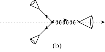
Figure 1: Event pictures of (a) two-jet configurations from quark-antiquark final states and (b) three-jet configurations originating from $q\bar{q}g$ events where the gluon is the hardest parton. The cones represent coherent soft and collinear gluon emission. The thrust axis is denoted by a dashed line.

3 The probabilistic interpretation

We can apply the coherent branching formalism to event shapes in the following schematic way illustrated in Fig. 1. The underlying configuration in e⁺e^- annihilation is the production of a quark-antiquark pair aligned with the thrust axis (Fig. 1(a)). Each parton then undergoes soft and collinear gluon emission (denoted by the open cone at the head of the parton). This contribution describes small angle and soft emission accurately in two-jet-like events when $B_{W}$ and $\rho_{H}$ are small and gives rise to the exponentiated first term in Eq. (6). However, it does not describe the possibility of wide angle gluon emission shown in Fig. 1(b) where the gluon is the hardest parton. This three-jet-like matrix element correction is not logarithmically enhanced at ${\cal O}(\alpha_{s})$ and first contributes at next-to-next-to-leading logarithmic accuracy and can therefore be neglected.

Let us first focus on the hemisphere masses. To next-to-leading logarithmic accuracy, the fraction of events with heavy hemisphere mass less than $\rho_{H}$ i.e. $k_{1}^{2}<\rho_{H}Q^{2}$ and $k_{2}^{2}<\rho_{H}Q^{2}$ is given by the two jet contribution

$$R_{H}(\rho_{H},\alpha_{s}(Q^{2}))\ \mathop{=}_{\rho_{H}\ll 1}$$ (15)

$$\int\limits^{\infty}_{0}\mathrm{d}k_{1}^{2}\int\limits^{\infty}_{0}\mathrm{d}k_{2}^{2}\ J^{q}(Q^{2},k_{1}^{2})\ J^{q}(Q^{2},k_{2}^{2})\ \Theta(\rho_{H}Q^{2}-k_{1}^{2})\ \Theta(k_{1}^{2}-k_{2}^{2})$$

$$+\int\limits^{\infty}_{0}\mathrm{d}k_{1}^{2}\int\limits^{\infty}_{0}\mathrm{d}k_{2}^{2}\ J^{q}(Q^{2},k_{1}^{2})\ J^{q}(Q^{2},k_{2}^{2})\ \Theta(\rho_{H}Q^{2}-k_{2}^{2})\ \Theta(k_{2}^{2}-k_{1}^{2}),$$

and where the constraint that $\rho_{H}\ll 1$ has suppressed the three and more jet contributions. Following the steps of Ref. [5], we can rewrite this formula using the phase space restrictions as

$$R_{H}(\rho_{H},\alpha_{s}(Q^{2}))\ \mathop{=}_{\rho_{H}\ll 1}\left[\Sigma^{q}_{H}(\rho_{H},\alpha_{s}(Q^{2}))\right]^{2}.$$ (16)

where

$$\Sigma^{q}_{H}(\rho_{H},\alpha_{s}(Q^{2}))=\int\limits^{\rho_{H}Q^{2}}_{0}\mathrm{d}k^{2}\ J^{q}(Q^{2},k^{2}).$$ (17)

The fraction of events with light hemisphere mass less than $\rho_{L}$ also receives contributions from the two-jet configuration when $k_{1}^{2}<\rho_{L}Q^{2}$ and $k_{2}^{2}>k_{1}^{2}$ and vice versa. Altogether we have,

$$R_{L}(\rho_{L},\alpha_{s}(Q^{2}))\ \mathop{=}_{\rho_{L}\ll 1}$$ (18)

$$\int\limits^{\infty}_{0}\mathrm{d}k_{1}^{2}\int\limits^{\infty}_{0}\mathrm{d}k_{2}^{2}\ J^{q}(Q^{2},k_{1}^{2})\ J^{q}(Q^{2},k_{2}^{2})\ \Theta(\rho_{L}Q^{2}-k_{1}^{2})\ \Theta(k_{2}^{2}-k_{1}^{2})$$

$$+\int\limits^{\infty}_{0}\mathrm{d}k_{1}^{2}\int\limits^{\infty}_{0}\mathrm{d}k_{2}^{2}\ J^{q}(Q^{2},k_{1}^{2})\ J^{q}(Q^{2},k_{2}^{2})\ \Theta(\rho_{L}Q^{2}-k_{2}^{2})\ \Theta(k_{1}^{2}-k_{2}^{2}).$$

Simplifying the phase space constraints, we find

$$R_{L}(\rho_{L},\alpha_{s}(Q^{2}))\ \mathop{=}_{\rho_{L}\ll 1}2~{}\Sigma^{q}_{H}(\rho_{L},\alpha_{s}(Q^{2}))-\left[\Sigma^{q}_{H}(\rho_{L},\alpha_{s}(Q^{2}))\right]^{2}.$$ (19)

The functions that resum the logarithms for the light hemisphere mass are the same as those that resum the logarithms for the heavy hemisphere mass. Now however, exponentiation in its purest form is spoiled because the final result is a sum of terms.

The analysis for the narrow jet broadening proceeds in the same way. We find that $R_{N}$, the probability of finding an event with a light hemisphere mass less than $B_{N}$, is given by

$$R_{N}(B_{N},\alpha_{s}(Q^{2}))\ \mathop{=}_{B_{N}\ll 1}2~{}\Sigma^{q}_{W}(B_{N},\alpha_{s}(Q^{2}))-\left[\Sigma^{q}_{W}(B_{N},\alpha_{s}(Q^{2}))\right]^{2}$$ (20)

where the probability of obtaining a jet with summed scalar transverse momentum $p_{t}$ with respect to the jet axis less than $2BQ$ starting from a parton of type $a$, $\Sigma^{a}_{W}$, is given by,

$$\Sigma^{a}_{W}(B,\alpha_{s}(Q^{2})=\int_{0}^{2BQ}T^{a}(Q,\mathbf{0},p_{t})dp_{t}.$$ (21)

4 All-orders resummation of large logarithms

In this section we discuss the all-orders resummation of leading logarithms ${\cal O}(\alpha_{s}^{n}L^{2n})$ and next-to-leading ${\cal O}(\alpha_{s}^{n}L^{2n-1})$ logarithms to all orders in the coupling constant. From eqs. (19) and (20), we see that to determine $R_{L}$ and $R_{N}$ requires knowledge of $\Sigma^{a}_{H}$ and $\Sigma^{a}_{W}$ respectively. Both of these functions have the exponentiated form of Eq. (6) and the corresponding functions $g_{1}(\alpha_{s}L)$ and $g_{2}(\alpha_{s}L)$ determined.

Explicit expressions for $\Sigma_{H}$ valid to this order are given in [3] and, introducing the renormalisation scale dependence in the standard manner and dropping the parton index, we reproduce them here for illustrative purposes,

$$\Sigma_{H}(\rho,\alpha_{s}(\mu^{2}),\mbox{$\frac{Q^{2}}{\mu^{2}}$}) = \frac{\exp[\mathcal{F}(\alpha_{s}(\mu^{2}),L)]}{\Gamma[1-\mathcal{S}(\alpha_{s}(\mu^{2}),L)]}$$ (22)

$$= \frac{\exp[Lf_{1}(x)+f_{2}(x)+x^{2}f_{1}^{\prime}(x)\ln(\mu^{2}/Q^{2})]}{\Gamma[1-f_{1}(x)-xf_{1}^{\prime}(x)]}+{\cal O}(\alpha_{s}^{n}L^{n-1})$$

where

$$L=\ln(1/\rho),\qquad x=\beta_{0}\alpha_{s}(\mu^{2})L.$$ (23)

The functions $f_{1}$, $f_{2}$ and $f_{1}^{\prime}$ are

$$f_{1}(x) = -\frac{A^{(1)}}{2\pi\beta_{0}x}\Biggl{[}(1-2x)\ln(1-2x)-2(1-x)\ln(1-x)\Biggr{]},$$ (24)

$$f_{2}(x) = -\frac{A^{(2)}}{2\pi^{2}\beta_{0}^{2}}\Biggl{[}2\ln(1-x)-\ln(1-2x)\Biggr{]}$$

$$+\frac{B^{(1)}}{2\pi\beta_{0}}\ln(1-x)-\frac{A^{(1)}\gamma_{E}}{\pi\beta_{0}}\Biggl{[}\ln(1-x)-\ln(1-2x)\Biggr{]}$$

$$-\frac{A^{(1)}\beta_{1}}{2\pi\beta_{0}^{3}}\Biggl{[}\ln(1-2x)-2\ln(1-x)+\frac{1}{2}\ln^{2}(1-2x)-\ln^{2}(1-x)\Biggr{]},$$

$$f_{1}^{\prime}(x) = \frac{A^{(1)}}{2\pi\beta_{0}x^{2}}\Biggl{[}\ln(1-2x)-2\ln(1-x)\Biggr{]},$$ (26)

with

$$\beta_{0}=\frac{11C_{A}-2N{\!{}_{f}}}{12\pi},\qquad\beta_{1}=\frac{17{C_{A}}^{2}-5C_{A}N{\!{}_{f}}-3C_{F}N{\!{}_{f}}}{24\pi^{2}},$$ (27)

For quarks,

$$A^{(1)}=C_{F},\qquad A^{(2)}=\frac{1}{2}C_{F}K,\qquad B^{(1)}=-\frac{3}{2}C_{F},$$ (28)

with $K$ given by Eq. (13).

Altogether Eqs. (22) to (28) are sufficient to determine $R_{N}$ of Eq. (20) to next-to-leading logarithmic accuracy. The expression for $R_{N}$ therefore correctly sums to all orders in the strong coupling, $\alpha_{s}$, only the leading two towers of large logarithms from ${\cal O}(\alpha_{s}^{n}L^{2n})$ down to ${\cal O}(\alpha_{s}^{n}L^{2n-1})$.

The resummed formula (19) does not include the ${\cal O}(\alpha_{s}^{2}L^{2})$ or ${\cal O}(\alpha_{s}^{2}L)$ terms (just as the analogous formulae for resumming three jet variables do not include the ${\cal O}(\alpha_{s}^{2}L^{2})$ or ${\cal O}(\alpha_{s}^{2}L)$ terms) present in the lowest order perturbative coefficient. Similarly, it does not produce the ${\cal O}(\alpha_{s}^{3}L^{4})$ to ${\cal O}(\alpha_{s}^{3}L)$ terms that occur in the next-to-leading order perturbative coefficient. The perturbative calculation provides the $\alpha_{s}^{2}$ and $\alpha_{s}^{3}$ contributions exactly and therefore the most significant omitted term is ${\cal O}(\alpha_{s}^{4}L^{6})$, see Fig. 2.

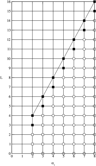
Figure 2: The towers of infrared logarithms appearing in the four-jet event shape rates $R_{L}$ and $R_{N}$. The resummation includes the leading and next-to-leading logarithms denoted by filled squares and the complete ${\cal O}(\alpha_{s}^{2},\alpha_{s}^{3})$ contributions from fixed order denoted by the empty squares. All other terms are incomplete and denoted by empty circles. The black filled squares denote terms generated purely in the two-jet limit.

Precisely the same discussion applies to the narrow jet broadening. Using the coherent branching formalism the functions $g_{1}(\alpha_{s}L)$ and $g_{2}(\alpha_{s}L)$ have been determined for $\Sigma_{W}$ and Catani et al (CTW) have provided analogous expressions for $\Sigma_{W}$ that are given in [5]. However, in doing so certain simplifying approximations concerning the recoil transverse momentum have been made. Dokshitzer and collaborators [19] have found that treating the quark recoil more carefully causes the CTW result for $\Sigma_{W}$ to be adjusted by a multiplicative factor. This modifies $g_{2}(\alpha_{s}L)$ but leaves $G_{11}$ unchanged. The same correction is in principle needed for the narrow jet broadening but is relevant beyond the next-to-leading logarithmic accuracy. Nevertheless, we chose to apply the correction to the CTW result. We do not give the final form for $\Sigma_{W}$ here, but instead refer the interested reader to Ref. [19]. Inserting the recoil-corrected form for $\Sigma_{W}$ in the resummed expression for $R_{N}$ (20) again allows resummation of the leading and next-to-leading logarithms as shown in Fig. 2.

5 Numerical results

As usual, the resummed result contains part of the fixed order perturbative contribution and the overlap must be removed by matching. This is done by expanding the resummed result as a series in the strong coupling constant and explicitly removing the terms corresponding to the fixed order calculations. This can be achieved in several ways of which $R$ matching and $\ln(R)$ matching are the most common. In the $R$ matching scheme, the coefficients of each of the unsummed logarithms present in the fixed order perturbative coefficients must be numerically extracted. For the four-jet event shape observables discussed here, this corresponds to determining the coefficient of $\alpha_{s}^{2}L$ from the lowest order perturbative contribution and the coefficients of $\alpha_{s}^{3}L^{2}$ and $\alpha_{s}^{3}L$ from the next-to-leading order contribution. This is impractical. However, in the more commonly used $\ln(R)$ matching scheme, it is assumed that the fixed order result exponentiates and therefore it is not necessary to make this extraction because any logarithmic terms remaining after subtracting the overlap from the fixed order contribution are exponentially suppressed. Of course, for the four-jet variables considered here, $R$ does not exponentiate. Nevertheless, in the $\ln(R)$ matching procedure, any remaining logarithmic terms are still exponentially suppressed. We therefore employ the $\ln(R)$ matching procedure.

To be more precise, the resummed result has the form

$$R_{resummed}=\mathcal{C}_{1}2\Sigma-\mathcal{C}_{2}\Sigma^{2}+{\cal O}(\alpha_{s}),$$ (29)

where $\mathcal{C}_{i}$ are power series in $\alpha_{s}$ and ${\cal O}(\alpha_{s})$ represents the contribution from three-jet configurations. The ${\cal O}(\alpha_{s})$ term of $\mathcal{C}_{1}$ and $\mathcal{C}_{2}$ are related by the constraint that there can be no logarithmic contributions at ${\cal O}(\alpha_{s})$ - the expansion of $R$ containing logarithms starts at ${\cal O}(\alpha_{s}^{2})$. However, to the next-to-leading logarithmic accuracy relevant for this paper, we can set $\mathcal{C}_{1}=\mathcal{C}_{2}=1$. The $\ln{R}$ matching formula then dictates that

$$\ln(R)=\ln(R_{resummed})+\ln(R_{fixed})-\ln(R_{expanded}),$$ (30)

where $\ln{R_{fixed}}$ and $\ln{R_{expanded}}$ are obtained by expanding the fixed order result and the $\ln{R_{resummed}}$ through to ${\cal O}(\alpha_{s}^{3})$ respectively. Using the expansion of $\ln(\Sigma)$ as a series,

$$\ln(\Sigma)=\sum_{n=1}^{\infty}\sum_{m=1}^{n+1}G_{nm}\alpha_{s}^{n}L^{m},$$

and with $\mathcal{C}_{1}=\mathcal{C}_{2}=1$, we see that,

$$\ln(R_{expanded}) = -(G_{11}L+G_{12}L^{2})^{2}\alpha_{s}^{2}$$ (31)

$$-2(G_{11}L+G_{12}L^{2})(G_{21}L+G_{22}L^{2}+G_{23}L^{3}+\frac{1}{2}(G_{11}L+G_{12}L^{2})^{2})\alpha_{s}^{3}$$

$$+{\cal O}(\alpha_{s}^{4}).$$

At next-to-leading logarithmic accuracy, logarithmic terms from the fixed order contribution remain in $\ln(R)$ given by Eq. (30), however, they are exponentially suppressed when translated back to $R$.

We expect that at large values of the observable $O$ the resummed result is dominated by the fixed order calculation. However, the resummed expressions (19) and (20) valid in the small $\rho_{L}$ and $B_{N}$ limits do not contain information about the kinematic endpoints of the distributions. To ensure that the resummed result vanishes at the endpoint we make the substitution

$$\frac{1}{O}\to\frac{1}{O}-\frac{1}{O^{\rm max}}+1,$$ (32)

where $O^{\rm max}$ corresponds to the endpoint of the distribution at the accuracy of the fixed order calculation. We use $\rho_{L}^{\rm max}=0.167$ and $B_{N}^{\rm max}=0.204$.

Numerical results for the light hemisphere mass and for the narrow jet broadening are shown in figures 3 and 4 respectively. Throughout we set $\mu=Q=M_{Z}$ and use $\alpha_{s}(M_{Z})=0.118$ corresponding to the current world average. The next-to-leading order result which diverges at small values of the event shapes is taken from [13] and is evaluated at $\mu=Q$.

Figures 3 and 4 show that the resummations are extremely important for $\rho_{L}<0.01$ and $B_{N}<0.02$. Rather than the divergent fixed order prediction, we have the more physical resummed result that the probability of finding events with no radiation (very small values of $\rho_{L}$ and $B_{N}$) are vanishingly small. For the reference value of $\mu=Q$, the peak position of the $\rho_{L}$ distribution occurs at $\rho_{L}=0.01$ with a height of 0.33, while for $B_{N}$ the peak occurs at $B_{N}=0.02$ with a value of 0.48. At larger values, the resummation changes the NLO prediction by a more moderate amount indicating that uncalculated higher order corrections are under control. At very large values of $O$, the resummed and NLO predictions coincide because of the matching procedure of Eq. (32).

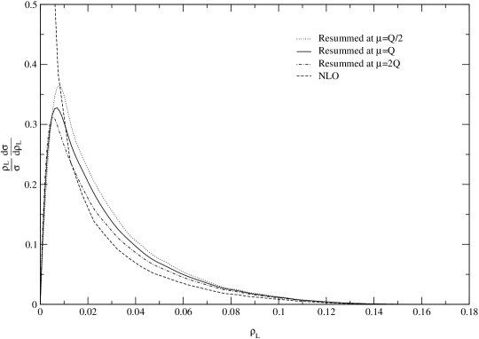
Figure 3: The resummed (solid) and fixed order NLO (dashed) predictions for the light hemisphere mass distribution $\frac{\rho_{L}}{\sigma}\frac{d\sigma}{d\rho_{L}}$ at $\mu=Q=M_{Z}$. The resummed prediction at $\mu=Q/2$ ($\mu=2Q$) is shown as a dotted (dot-dashed) curve.

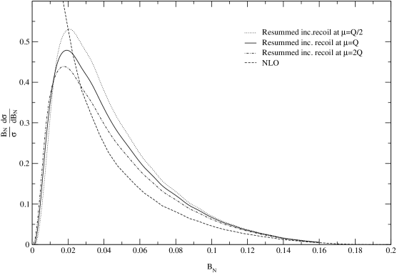
Figure 4: The resummed (solid) and fixed order NLO (dashed) predictions for the narrow jet broadening distribution $\frac{B_{N}}{\sigma}\frac{d\sigma}{dB_{N}}$ at $\mu=Q=M_{Z}$. The resummed prediction at $\mu=Q/2$ ($\mu=2Q$) is shown as a dotted (dot-dashed) curve.

To illustrate the residual renormalisation scale dependence, we also show the effect of varying $\mu$ by a factor of 2 either side of the reference value $\mu=Q$. We see that around the peak region, different scale choices alter the prediction by $\pm 10\%$.

The infrared resummation significantly improves the perturbative prediction for the event shape observable. However, when comparing with experimental data we should be aware that important non-perturbative hadronisation corrections are present. The effect of hadronisation on the distribution is to shift the value of the observable away from the two-jet region,

$$O\to O+O_{\rm NP},$$ (33)

where the non-perturbative correction depends on the typical hadron scale ${\cal O}(1~{}{\rm GeV})$ and is suppressed by a power of $Q$. In principle these power corrections can be estimated using the dispersive approach of Ref. [20] where a non-perturbative parameter $\mu_{I}$ is introduced to describe the running of $\alpha_{s}$ in the infrared region. For the associated three jet variables the non-perturbative corrections are typically estimated to be ${\cal O}(1~{}{\rm GeV}/Q)$ for $\rho_{H}$ [20] and ${\cal O}(0.3~{}{\rm GeV}\ln(1/B_{W})/Q)$ for $B_{W}$ [21] and arise through the hadronisation of one of the two jets in the event. Because the four-jet event shapes are largely related to what happens in the second jet, we might expect that the hadronisation corrections are similar. To illustrate the potential effects of hadronisation in the four-jet event shapes, we just transfer these corrections directly so that,

$$\rho_{L} \to \rho_{L}+\frac{1~{}{\rm GeV}}{Q},$$ (34)

$$B_{N} \to B_{N}+\frac{0.3~{}{\rm GeV}\ln(1/B_{N})}{Q}.$$ (35)

The simplified hadronisation correction applied to the resummed distributions for the light hemisphere mass and narrow jet broadening with $\mu=Q$ is shown in figures 5 and 6 respectively. To emphasize the dramatic effect the power correction has, we also show the uncorrected predictions. There are two effects. First the distribution is shifted to the right by an amount $O_{\rm NP}$ and second, the distribution is rescaled by a factor $(O+O_{\rm NP})/O$. In the region of the turnover where $O$ is of the same order as $O_{\rm NP}$ there is an enhancement of ${\cal O}$(100%). The hadronisation correction is smaller at larger values of $O$.

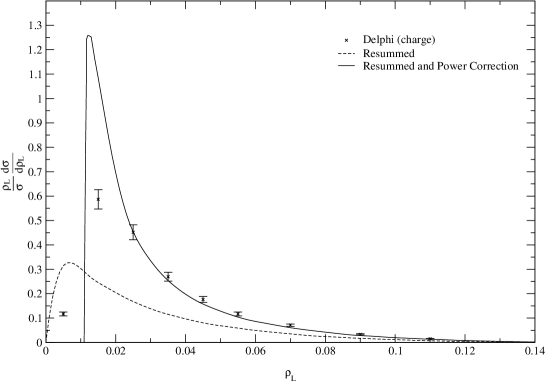
Figure 5: The resummed prediction for the light hemisphere mass distribution $\frac{\rho_{L}}{\sigma}\frac{d\sigma}{d\rho_{L}}$ at $\mu=Q=M_{Z}$ modified by a non-perturbative power correction $\rho_{L}\to\rho_{L}+1~{}{\rm GeV}/Q$. The resummed prediction without power correction is shown as a dashed line. For comparison, we also show the charged hadron data collected at the $Z$ resonance by the DELPHI collaboration [22].

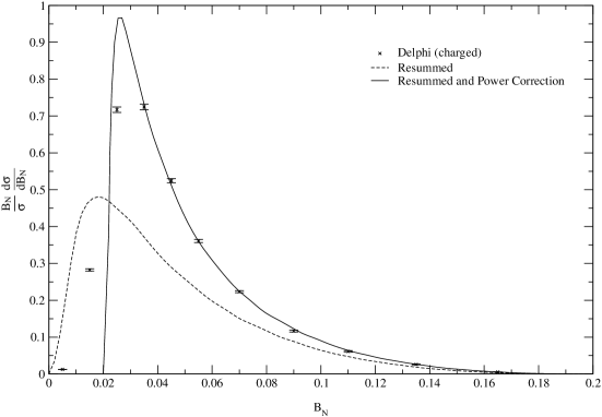
Figure 6: The resummed prediction for the narrow jet broadening distribution $\frac{B_{N}}{\sigma}\frac{d\sigma}{dB_{N}}$ at $\mu=Q=M_{Z}$ modified by a non-perturbative power correction $B_{N}\to B_{N}+0.3~{}{\rm GeV}\ln(1/B_{N})/Q$. The resummed prediction without power correction is shown as a dashed line. For comparison, we also show the charged hadron data collected at the $Z$ resonance by the DELPHI collaboration [22].

For comparison, we also show the charged hadron data collected by the DELPHI Collaboration [22] at the $Z$ resonance. We see remarkable agreement (strikingly so in view of the simplified hadronisation correction applied here). The only discrepancy is at very small values of $O<O_{\rm NP}$ where individual hadrons in the light/narrow hemisphere will significantly affect the value of $O$. We do not expect to successfully describe such events.

6 Conclusions

In this paper, we presented predictions for the light hemisphere mass and the narrow jet broadening distributions where the infrared logarithms have been resummed to next-to-leading logarithmic order using the coherent branching formalism. The resummed expressions do not exponentiate, but involve the difference of exponential factors so that the perturbative series starts at ${\cal O}(\alpha_{s}^{2})$. The expressions presented in sections 3 and 4 resum the leading ${\cal O}(\alpha_{s}^{n}L^{2n-1})$ and next-to-leading ${\cal O}(\alpha_{s}^{n}L^{2n-2})$ infrared logarithms to all orders in the coupling constant. Taken in conjunction with the fixed order ${\cal O}(\alpha_{s}^{3})$ non-logarithmic terms, the first neglected term is of ${\cal O}(\alpha_{s}^{4}L^{6})$. The numerical results shown in Figs. 3 and 4 indicate that the resummation effects are sizeable at small values of the event shape parameter and that the resummation procedure significantly improves the perturbative prediction.

However, because important non-perturbative hadronisation corrections are present, resummation alone is insufficient to describe the experimental data. Applying simple power corrections similar to those obtained for the heavy hemisphere mass and the wide jet broadening gives good qualitative agreement with the available data from LEP. We anticipate that the improved theoretical description of the four-jet event shape distributions presented here can be combined with a more sophisticated hadronisation correction based on the dispersive approach of Ref. [20]. The data from LEP can then be used to further test the structure of QCD in four-jet like events and extract values of the strong coupling constant.

References

- [1] R.K. Ellis, D.A. Ross and A.E. Terrano, Nucl. Phys. B178 (1981) 421.
- [2] S. Catani, G. Turnock, B.R. Webber and L. Trentadue, Phys. Lett. B263 (1991) 461; Nucl. Phys. B407 (1993) 3.
- [3] S. Catani and L. Trentadue, Phys. Lett. B217 (1989) 539; Nucl. Phys. B327 (1989) 323; Nucl. Phys. B353 (1991) 183; S. Catani, B.R. Webber and G. Marchesini, Nucl. Phys. B349 (1991) 635;
- [4] S. Catani, G. Turnock and B.R. Webber, Phys. Lett. B272 (1991) 368.
- [5] S. Catani, G. Turnock and B.R. Webber, Phys. Lett. B295 (1992) 269.
- [6] B.R. Webber, Phys. Lett. B339 (1994) 148 [hep-ph/9408222]; G.P. Korchemsky and G. Sterman, Nucl. Phys. B437 (1995) 415 [hep-ph/9411211]; Yu. L. Dokshitzer and B.R. Webber, Phys. Lett. B352 (1995) 451 [hep-ph/9504219]; R. Akhoury and V.I. Zakharov, Phys. Lett. B357 (1995) 646 [hep-ph/9504248]; R. Akhoury and V.I. Zakharov, Nucl. Phys. B465 (1996) 295 [hep-ph/9507253]; P. Nason and M.H. Seymour, Nucl. Phys. B454 (1995) 291 [hep-ph/9506317].
- [7] G. Dissertori, Nucl. Phys. Proc. Suppl. B 65 (1998) 43 [hep-ex/9705016] and references therein.
- [8] G. Dissertori, Nucl. Phys. Proc. Suppl. B 64 (1998) 46 and references therein.
- [9] A. Signer and L. Dixon, Phys. Rev. D56 (1997) 4031 [hep-ph/9706285].
- [10] Z. Nagy and Z. Trócsányi, Phys. Rev. D57 (1998) 3604 [hep-ph/9806317].
- [11] S. Weinzierl and D.A. Kosower, Phys. Rev. D60 (1999) 054028 [hep-ph/9901277]
- [12] Z. Bern, L. Dixon, D.A. Kosower and S. Weinzierl, Nucl. Phys. B489 (1997) 3 [hep-ph/9610370]; Z. Bern, L. Dixon and D.A. Kosower, Nucl. Phys. B513 (1998) 3 [hep-ph/9708239].
- [13] J.M. Campbell, M.A. Cullen and E.W.N. Glover, Eur. Phys. J. C9 (1999) 245 [hep-ph/9809429].
- [14] E.W.N. Glover and D.J. Miller, Phys. Lett. B396 (1997) 257 [hep-ph/9609474]; J.M. Campbell, E.W.N. Glover and D.J. Miller, Phys. Lett. B409 (1997) 503 [hep-ph/9706297].
- [15] S. Catani, Yu.L. Dokshitzer, M. Olsson, G. Turnock and B.R. Webber, Phys. Lett. B269 (1991) 432; S.J. Burby, Phys. Lett. B453 (1999) 54 [hep-ph/9902305].
- [16] A. Banfi, Yu.L. Dokshitzer, G. Marchesini and G. Zanderighi, JHEP 0007 (2000) 2 [hep-ph/0004027].
- [17] A. Banfi, Yu.L. Dokshitzer, G. Marchesini and G. Zanderighi, hep-ph/0010267, hep-ph/0101205.
- [18] L. Clavelli, Phys. Lett. B85 (1979) 111.
- [19] Yu. L. Dokshitzer, A. Lucenti, G. Marchesini and G.P. Salam, JHEP 9801 (1998) 11 [hep-ph/9801324].
- [20] Yu. L. Dokshitzer, G. Marchesini and B.R. Webber, Nucl. Phys. B469 (1996) 93 [hep-ph/9512336]; Yu. L. Dokshitzer and B.R. Webber, Phys. Lett. B404 (1997) 321 [hep-ph/9704298].
- [21] Yu. L. Dokshitzer, G. Marchesini and G.P. Salam, Eur. Phys. J. C3 (1999) 1 [hep-ph/9812487].
- [22] P. Abreu et al, DELPHI Collaboration, Z. Phys. C73 (1996) 11.