THE SPIN STRUCTURE OF THE NUCLEON

Abstract

We present an overview of recent experimental and theoretical advances in our understanding of the spin structure of protons and neutrons.

^∗W. K. Kellogg Laboratory, California Institute of Technology,

Pasadena, CA 91125

^∗∗Department of Physics, University of Maryland,

College Park, MD 20742

1 Introduction

Attempting to understand the origin of the intrinsic spin of the proton and neutron has been an active area of both experimental and theoretical research for the past twenty years. With the confirmation that the proton and neutron were not elementary particles, physicists were challenged with the task of explaining the nucleon’s spin in terms of its constituents. In a simple constituent picture one can decompose the nucleon’s spin as

$$J_{z}^{N}=S_{z}^{q}+L_{z}^{q}+S_{z}^{g}+L_{z}^{g}={1\over 2}\ .$$ (1)

where $S_{z}$ and $L_{z}$ represent the intrinsic and orbital angular momentum respectively for quarks and gluons. A simple non-relativistic quark model (as described below) gives directly $S_{z}^{q}={1\over 2}$ and all the other components $=0$.

Because the structure of the nucleon is governed by the strong interaction, the components of the nucleon’s spin must in principle be calculable from the fundamental theory: Quantum Chromodynamics (QCD). However since the spin is a low energy property, direct calculations with non-perturbative QCD are only possible at present with primitive lattice simulations. The fact that the nucleon spin composition can be measured directly from experiments has created an important frontier in hadron physics phenomenology and has had crucial impact on our basic knowledge of the internal structure of the nucleon.

This paper summarizes the status of our experimental and theoretical understanding of the nucleon’s spin structure. We begin with a simplified discussion of nucleon spin structure and how it can be accessed through polarized Deep Inelastic Scattering (DIS). This is followed by a theoretical overview of spin structure in terms of QCD. The experimental program is then reviewed where we discuss the vastly different techniques being applied in order to limit possible systematic errors in the measurements. We then address the variety of spin distributions associated with the nucleon: the total quark helicity distribution $\Delta\Sigma$ extracted from inclusive scattering, the individual quark helicity distributions (flavor separation) determined by semi-inclusive scattering, and the gluon helicity distribution accessed by a variety of probes. We also discuss some additional distributions that have have recently been discussed theoretically but are only just being accessed experimentally: the transversity distribution and the off-forward distributions. Lastly we review a few topics closely related to the spin structure of the nucleon.

A number of reviews of nucleon spin structure have been published. Following the pioneering review of the field by Hughes and Kuti [177] which set the stage for the very rapid development over the last fifteen years, a number of reviews have summarized the recent developments [77, 43, 216, 176, 105]. Also Ref. [91] presents a detailed review of the potential contribution of the Relativistic Heavy Ion Collider (RHIC) to field of nucleon spin structure.

1.1 A Simple Model for Proton Spin

A simple non-relativistic wave function for the proton comprising only the valence up and down quarks can be written as

$$|p\uparrow\rangle={1\over\sqrt{6}}(2|u\uparrow u\uparrow d\downarrow\rangle-|u\uparrow u\downarrow d\uparrow\rangle-|u\downarrow u\uparrow d\uparrow\rangle.$$ (2)

where we have suppressed the color indices and permutations for simplicity but enforced the normalization. Here the up and down quarks give all of the proton’s spin. The contribution of the $u$ and $d$ quarks to the proton’s spin can be determined by the use of the following matrix element and projection operator:

$$u^{\uparrow}=\langle p\uparrow|\hat{\mathcal{O}}_{u\uparrow}|p\uparrow\rangle$$ (3)

$$\hat{\mathcal{O}}_{u\uparrow}={1\over 4}(1+\hat{\tau}_{3})(1+\hat{\sigma}_{3})\ .$$ (4)

where the matrix element gives the number of up quarks polarized along the direction of the proton’s polarization. With the above matrix element and a similar one for the down quarks, the quark spin contributions can be defined as

$$\Delta u=u^{\uparrow}-u^{\downarrow}={1\over 2}(\langle\sigma_{3}\rangle+\langle\sigma_{3}\tau_{3}\rangle)={4\over 3}\ ,$$ (5)

$$\Delta d=d^{\uparrow}-d^{\downarrow}={1\over 2}(\langle\sigma_{3}\rangle-\langle\sigma_{3}\tau_{3}\rangle)=-{1\over 3}\ .$$ (6)

Thus the fraction of the proton’s spin carried by quarks in this simple model is

$$\Delta\Sigma\equiv\Delta u+\Delta d+\Delta s=\langle\sigma_{3}\rangle=2J_{z}^{N}=1\ ,$$ (7)

and all of the spin is carried by the quarks. Note however that this simple model overestimates another property of the nucleon, namely the axial-vector weak coupling constant $g_{A}$. In fact this model gives

$${g_{A}\over g_{V}}=\langle\sigma_{3}\tau_{3}\rangle=\Delta u-\Delta d={5\over 3}\ ,$$ (8)

compared to the experimentally measured value of ${g_{A}/g_{V}}=1.267\pm 0.004$. The difference between the simple non-relativistic model and the data is often attributed to relativistic effects. This “quenching” factor of $\sim$ 0.75 can be applied to the spin carried by quarks to give the following “relativistic” constituent quark model predictions:

$$\Delta\Sigma\approx 0.75\ ,$$

$$\Delta u\approx 1.0\ ,$$

$$\Delta d\approx -0.25\ ,$$

$$\Delta s\approx 0\ .$$ (9)

1.2 Lepton Scattering as a Probe of Spin Structure

Deep-inelastic scattering (DIS) with charged lepton beams has been the key tool for probing the structure of the nucleon. With polarized beams and targets the ${\it spin}$ structure of the nucleon becomes accessible. Information from neutral lepton scattering (neutrinos) is complementary to that from charged leptons but is generally of lower statistical quality.

Figure 1: Deep Inelastic Scattering in the Quark-Parton Model

The access to nucleon structure through lepton scattering can best be seen within the Quark-Parton Model (QPM). An example of a deep-inelastic scattering process is shown in Fig. 1. In this picture a virtual photon of four-momentum $q^{\mu}$(with energy $\nu$ and four-momentum transfer $Q^{2}\equiv-q^{2}$) strikes an asymptotically free quark in the nucleon. We are interested in the deep-inelastic (Bjorken) limit in which $Q^{2}$ and $\nu$ are large, while the Bjorken scaling variable $x_{B}=Q^{2}/2M\nu$ is kept fixed ($M$ is the nucleon mass). For unpolarized scattering the quark “momentum” distributions—$q_{i}(x)=u(x),d(x),s(x),$ … — are probed in this reaction, where $x=x_{B}$ is the quark’s momentum fraction. From the cross section for this process, the structure function $F_{1}(x)$ can be extracted. In the quark-parton model this structure function is related to the unpolarized quark distributions via

$$F_{1}(x)={1\over 2}\sum_{i}e_{i}^{2}q_{i}(x)\ ,$$ (10)

where the sum is over both quark and anti-quark flavors. With polarized beams and targets the quark spin distributions can be probed. This sensitivity results from the requirement that the quark’s spin be anti-parallel to the virtual photon’s spin in order for the quark to absorb the virtual photon. With the assumption of nearly massless and collinear quarks, angular momentum would not be conserved if the quark absorbs a photon when its spin is parallel to the photon’s spin. Thus measurements of the spin-dependent cross section allow the extraction of the spin-dependent structure function $g_{1}(x)$. Again in the quark-parton model this structure function is related to the quark spin distributions via

$$g_{1}(x)={1\over 2}\sum_{i}e_{i}^{2}\Delta q_{i}(x)\ .$$ (11)

The structure function $g_{1}$ is extracted from the measured asymmetries of the scattering cross section as the beam or target spin is reversed. These asymmetries are measured with longitudinally polarized beams and longitudinally ($A_{||})$ and transversely ($A_{\perp}$) polarized targets (see Sec. 3).

Beyond the QPM, QCD introduces a momentum scale ($Q^{2}$) dependence into the structure functions (eg. $F_{1}(x,Q^{2})$ and $g_{1}(x,Q^{2})$). The calculation of this $Q^{2}$ dependence is based on the Operator Product Expansion (OPE) and the renormalization group equations (see eg. Ref. [261, 180, 43]). We will not discuss this in detail, but we will use some elements of the expansion. In particular, the expansion can be written in terms of “twist” which is the difference between the dimension and the spin of the operators that form the basis for the expansion. The matrix elements of these operators cannot be calculated in perturbative QCD, but the corresponding $Q^{2}$-dependent coefficients are calculable. The lowest order coefficients (twist-two) remain finite as $Q^{2}\rightarrow\infty$ while the higher-twist coefficients vanish as $Q^{2}\rightarrow\infty$ (due to their $1/Q^{2}$ dependence). Therefore, the full $Q^{2}$ dependence includes both QCD radiative corrections (calculated to next-to-leading-order (NLO) at present) and higher-twist corrections. The NLO corrections will be discussed in Sec. 3.5.

1.3 Theoretical Introduction

To go beyond the simple picture of nucleon spin structure discussed above we must address the spin structure within the context of QCD. We discuss several of these issues in the following sections.

1.3.1 Quark Helicity Distributions and $g_{1}(x,Q^{2})$

In polarized DIS, the antisymmetric part of the nucleon tensor is measured,

$$W_{\mu\nu}={1\over 4\pi}\int e^{i\xi\cdot q}d^{4}\xi\langle PS|[J_{\mu}(\xi),J_{\nu}(0)|PS\rangle\ ,$$ (12)

where $|PS\rangle$ is the ground state of the nucleon with four-momentum $P^{\mu}$ and polarization $S^{\mu}$ ($P\cdot S=0$), and $J^{\mu}$ is the electromagnetic current. The antisymmetric part can be expressed in terms of two invariant structure functions,

$$W^{[\mu\nu]}=-i\epsilon^{\mu\nu\alpha\beta}q_{\alpha}\left[G_{1}(\nu,Q^{2})S_{\beta}/M^{2}+G_{2}(\nu,Q^{2})(S_{\beta}\nu M-P_{\beta}S\cdot q)/M^{4}\right]\ .$$ (13)

In the Bjorken limit, we obtain two scaling functions,

$$g_{1}(x,Q^{2}) = \left({\nu\over M}\right)G_{1}(\nu,Q^{2})\ \rightarrow\ g_{1}(x)\ ,$$

$$g_{2}(x,Q^{2}) = \left({\nu\over M}\right)^{2}G_{2}(\nu,Q^{2})\ \rightarrow\ g_{2}(x)\ ,$$ (14)

which are non-vanishing.

If the QCD radiative corrections are neglected, $g_{1}(x,Q^{2})$ is related to the polarized quark distributions $\Delta q(x)$ as shown in Eq. (11). In QCD, the distribution can be expressed as the Fourier transform of a quark light-cone correlation,

$$\Delta q(x,\mu^{2})={1\over 2}\int{d\lambda\over 2\pi}e^{i\lambda x}\langle PS|\overline{\psi}(0)U(0,\lambda n)\not\!n\gamma_{5}\psi(\lambda n)|PS\rangle$$ (15)

where $n$ is a light-cone vector (eg. $n=(1,0,0,-1)$) and $\mu^{2}$ is a renormalization scale. $U(0,\lambda n)=\exp(-ig\int^{0}_{\lambda}n\cdot A(\mu n)d\mu)$ is a path-ordered gauge link making the operator gauge invariant. When QCD radiative corrections are taken into account, the relation between $g_{1}(x,Q^{2})$ and $\Delta q(x,\mu^{2})$ is more complicated (see Sec. 3.5). When $Q^{2}$ is not too large ($<5$ GeV²), one must take into account the higher-twist contributions to $g_{1}(x,Q^{2})$, which appear as $1/Q^{2}$ power corrections. Some initial theoretical estimates of these power corrections have been performed [62, 198].

Integrating the polarized quark distributions over $x$ yields the fraction of the nucleon spin carried by quarks,

$$\Delta\Sigma=\int^{1}_{0}dx\sum_{i}\left(\Delta q_{i}(x)+\Delta\bar{q}_{i}(x)\right)\ .$$ (16)

The individual quark contribution $\Delta q$ is also called the axial charge because it is related to the matrix element of the axial current $\bar{\psi}\gamma_{\mu}\gamma_{5}\psi$ in the nucleon state. $\Delta\Sigma$ is the singlet axial charge. Because of the axial anomaly, it is a scale-dependent quantity.

1.3.2 The Nucleon Spin Sum Rule

To understand the spin structure of the nucleon in the framework QCD, we can write the QCD angular momentum operator in a gauge-invariant form [186]

$$\vec{J}_{\rm QCD}=\vec{J}_{q}+\vec{J}_{g}\,,$$ (17)

where

$$\vec{J}_{q} = \int d^{3}x~{}\vec{x}\times\vec{T}_{q}$$

$$= \int d^{3}x~{}\left[\psi^{\dagger}{\vec{\Sigma}\over 2}\psi+\psi^{\dagger}\vec{x}\times(-i\vec{D})\psi\right]\,,$$

$$\vec{J}_{g} = \int d^{3}x~{}\vec{x}\times(\vec{E}\times\vec{B})\,.$$ (18)

(The angular momentum operator in a gauge-variant form has also motivated a lot of theoretical work, but is unattractive both theoretically and experimentally [253].) The quark and gluon components of the angular momentum are generated from the quark and gluon momentum densities $\vec{T}_{q}$ and $\vec{E}\times\vec{B}$, respectively. $\vec{\Sigma}$ is the Dirac spin matrix and the corresponding term is the quark spin contribution. $\vec{D}=\vec{\nabla}-ig\vec{A}$ is the covariant derivative and the associated term is the gauge-invariant quark orbital angular momentum contribution.

Using the above expression, one can easily construct a sum rule for the spin of the nucleon. Consider a nucleon moving in the $z$ direction, and polarized in the helicity eigenstate $\lambda=1/2$. The total helicity can be evaluated as an expectation value of $J_{z}$ in the nucleon state,

$${1\over 2}={1\over 2}\Delta\Sigma(\mu)+L_{q}(\mu)+J_{q}(\mu)\,,$$ (19)

where the three terms denote the matrix elements of three parts of the angular momentum operator in Eq. 18. The physical significance of each term is obvious, modulo the momentum transfer scale $Q^{2}$ and scheme dependence (see Sec. 3.5) indicated by $\mu$. There have been attempts to remove the scale dependence in $\Delta\Sigma$ by subtracting a gluon contribution [37]. Unfortunately, such a subtraction is by no means unique. Here we adopt the standard definition of $\Delta\Sigma(\mu)$ as the matrix element of the multiplicatively renormalized quark spin operator. As has been discussed above, $\Delta\Sigma(\mu)$ can be measured from polarized deep-inelastic scattering and the measurement of the other terms will be discussed in later sections. Note that the individual terms in the above equation are independent of the nucleon velocity [188]. In particular, the equation applies when the nucleon is traveling with the speed of light (the infinite momentum frame).

The scale dependence of the quark and gluon contributions can be calculated in perturbative QCD. By studying renormalization of the nonlocal operators, one can show [186, 253]

$${\partial\over\partial\ln\mu^{2}}\left(\begin{array}[]{c}J_{q}(\mu)\\ J_{g}(\mu)\end{array}\right)={\alpha_{s}(\mu)\over 2\pi}{1\over 9}\left(\begin{array}[]{rr}-16&3n_{F}\\ 16&-3n_{F}\\ \end{array}\right)\left(\begin{array}[]{c}J_{q}(\mu)\\ J_{g}(\mu)\end{array}\right)\ .$$ (20)

As $\mu\rightarrow\infty$, there exists a fixed-point solution

$$J_{q}(\infty) = {1\over 2}{3n_{f}\over 16+3n_{f}}\ ,$$

$$J_{g}(\infty) = {1\over 2}{16\over 16+3n_{f}}\ .$$ (21)

Thus as the nucleon is probed at an infinitely small distance scale, approximately one-half of the spin is carried by gluons. A similar result has been obtained by Gross and Wilczek in 1974 for the quark and gluon contributions to the momentum of the nucleon [164]. Strictly speaking, these results reveal little about the nonperturbative structure of bound states. However, experimentally it is found that about half of the nucleon momentum is carried by gluons even at relatively low energy scales (see eg. [214]). Thus the gluon degrees of freedom not only play a key role in perturbative QCD, but also are a major component of nonperturbative states as expected. An interesting question is then, how much of the nucleon spin is carried by the gluons at low energy scales? A solid answer from the fundamental theory is not yet available. Balitsky and Ji have made an estimate using the QCD sum rule approach [61]:

$$J_{g}(\mu\sim 1{\rm GeV})\simeq{8\over 9}{e<\bar{u}\sigma Gu><\bar{u}u>\over M_{1^{-+}}^{2}\lambda_{N}^{2}}$$ (22)

which yields approximately 0.25. Based on this calculation, the spin structure of the nucleon would look approximately like

$${1\over 2}=0.10({\rm from~{}}{1\over 2}\Delta\Sigma)+0.15({\rm from~{}}L_{q})+0.25({\rm from~{}}J_{g})\ .$$ (23)

Lattice [226] and quark model [65] calculations of $J_{q}$ have yielded similar results.

While $\Delta\Sigma$ has a simple parton interpretation, the gauge-invariant orbital angular momentum clearly does not. Since we are addressing the structure of the nucleon, it is not required that a physical quantity have a simple parton interpretation. The nucleon mass, magnetic moment, and charge radius do not have simple parton model explanations. The quark orbital angular momentum is related to the transverse momentum of the partons in the nucleon. It is well known that transverse momentum effects are beyond the naive parton picture. As will be discussed later, however, the orbital angular momentum does have a more subtle parton interpretation (see Sec. 7).

In the literature, there are suggestions that $\vec{r}\times(-i\nabla)$ be considered the orbital angular momentum [253]. This quantity is clearly not gauge invariant and $-i\nabla$ does not correspond to the velocity in classical mechanics [143]. Under scale evolution, this operator mixes with an infinite number of other operators in light-cone gauge [175]. More importantly, there is no known way to measure such “orbital angular momentum.”

1.3.3 Gluon Helicity Distribution $\Delta G(x,Q^{2})$

In a longitudinally-polarized nucleon the polarized gluon distribution $\Delta G(x,Q^{2})$ contributes to spin-dependent scattering processes and hence various experimental spin asymmetries. In QCD, using the infrared factorization of hard process, $\Delta G(x,Q^{2})$ with $-1<x<1$ can be expressed as

$$\Delta G(x,\mu^{2})={i\over 2}\int{d\lambda\over 2\pi}e^{i\lambda x}\langle PS|F^{+\alpha}(0)U(0,\lambda n)\tilde{F}^{+}_{~{}~{}\alpha}(\lambda n)|PS\rangle\ ,$$ (24)

where $\tilde{F}_{\alpha\beta}=(1/2)\epsilon_{\alpha\beta\mu\nu}F^{\mu\nu}$. Because of the charge conjugation property of the operator, the gluon distribution is symmetric in $x$: $\Delta G(x,Q^{2})=\Delta G(-x,Q^{2})$.

The even moments of $\Delta G(x,Q^{2})$ are directly related to matrix elements of charge conjugation even local operators. Defining

$$\int^{1}_{-1}dxx^{n-1}\Delta G(x,Q^{2})=a_{n}(\mu^{2})\ ,~{}~{}~{}(n=3,5\cdots)$$ (25)

we have

$$\langle PS|F^{\mu_{1}\alpha}iD^{\mu_{2}}\cdots iD^{\mu_{n-1}}i\tilde{F}^{\mu_{n}}_{~{}~{}\alpha}|PS\rangle =2a_{n}(\mu^{2})S^{\mu_{1}}P^{\mu_{2}}\cdots P^{\mu_{n}}$$

$$(n=3,5\cdots)\ .$$

The renormalization scale dependence is directly connected to renormalization of the local operators. Because Eq. (24) involves directly the time variable, it is difficult to evaluate the distribution on a lattice. However, the matrix elements of local operators are routinely calculated in lattice QCD, hence the moments of $\Delta G(x,Q^{2})$ are, in principle, calculable.

From the above equations, it is clear that the first-moment ($n=1$) of $\Delta G(x)$ does not correspond to a gauge-invariant local operator. In the axial gauge $n\cdot A=0$, the first moment of the nonlocal operator can be reduced to a local one, $\vec{E}\times\vec{A}$, which can be interpreted as the gluon spin density operator. As a result, the first moment of $\Delta G(x,\mu^{2})$ represents the gluon spin contribution to the nucleon spin in the axial gauge. In any other gauge, however, it cannot be interpreted as such. Thus one can formally write $J_{g}=\Delta G+L_{g}$ in the axial gauge, where $L_{g}$ is then the gluon orbital contribution the nucleon spin. There is no known way to measure $L_{g}$ directly from experiment other than defining it as the difference between $J_{g}$ and $\Delta G$.

2 Experimental Overview

A wide variety of experimental approaches have been applied to the investigation of the nucleon’s spin structure. The experiments complement each other in their kinematic coverage and in their sensitivity to possible systematic errors associated with the measured quantities. A summary of the spin structure measurements is shown in Table 1, where the beams, targets, and typical energies are listed for each experiment. The kinematic coverage of each experiment is indicated in the table by its average four-momentum transfer ($Q^{2}$) and Bjorken $x$ range (for $Q^{2}>1$ GeV²). Also given are the average or typical beam and target polarizations as quoted by each experimental group in their respective publications (or in their proposals for the experiments that are underway). The column labeled $f$ lists the dilution factor, which is the fraction of scattered events that result from the polarized atoms of interest, and the column labeled $\mathcal{L}$ is an estimate of the total nucleon luminosity (# of nucleons/cm${}^{2}\times$ # of beam particles/s) in units of $10^{32}$ nucleons/cm²/s for each experiment.

In an effort to eliminate possible sources of unknown systematic error in the measurements the experiments have been performed with significantly different experimental techniques. Examples of the large range of experimental parameters for the measurements include variations in the beam polarization of $40-80\%$, in the target polarization of $30-90\%$ and in the correction for dilution of the experimental asymmetry due to unpolarized material of $0.1-1$.

We now present an overview of the individual experimental techniques with an emphasis on the different approaches taken by the various experiments.

Table 1: Summary of High Energy Spin Structure Function Measurements.

Lab	Exp.	Year	Beam	$\langle Q^{2}\rangle$	$x$	$P_{B}$	Target	$P_{T}$	$f$	$\mathcal{L}\times 10^{-32}$
				GeV2						cm-2-s
SLAC	E80	75	10-16 GeV $e^{-}$	2	0.1 – 0.5	85%	H-butanol	50%	0.13	400
	E130	80	16-23 GeV $e^{-}$	5	0.1 – 0.6	81%	H-butanol	58%	0.15	400
	E142	92	19-26 GeV $e^{-}$	2	0.03 – 0.6	39%	3He	35%	0.35	2000
	E143	93	10-29 GeV $e^{-}$	3	0.03 – 0.8	85%	NH3	70%	0.15	1000
							ND3	25%	0.24	1000
	E154	95	48 GeV $e^{-}$	5	0.01 – 0.7	82%	3He	38%	0.55	3000
	E155	97	48 GeV $e^{-}$	5	0.01 – 0.9	81%	NH3	90%	0.15	1000
							LiD	22%	0.36	1000
	E155’	99	30 GeV $e^{-}$	3	0.02 – 0.9	83%	NH3	75%	0.16	1000
							LiD	22%	0.36	1000
CERN	EMC	85	100-200 GeV $\mu^{+}$	11	0.01 – 0.7	79%	NH3	78%	0.16	0.3
	SMC	92	100 GeV $\mu^{+}$	4.6	0.006 – 0.6	82%	D-butanol	35%	0.19	0.3
		93	190 GeV $\mu^{+}$	10	0.003 – 0.7	80%	H-butanol	86%	0.12	0.6
		94-95				81%	D-butanol	50%	0.20	0.6
		96				77%	NH3	89%	0.16	0.6
DESY	HERMES	95	28 GeV $e^{+}$	2.5	0.02 – 0.6	55%	3He	46%	1.0	1
		96-97				55%	H	88%	1.0	0.1
		98	28 GeV $e^{-}$			55%	D	85%	1.0	0.2
		99-00	28 GeV $e^{+}$			55%	D	85%	1.0	0.2
CERN	COMPASS	01	190 GeV $\mu^{+}$	10	0.005 – 0.6	80%	NH3	90%	0.16	3
							LiD	40%	0.50	3
BNL	RHIC	02	200 GeV p - p	$\sim 100$	0.05 – 0.6	70%	Collider	70%	1.0	2
DESY	ZEUS/H1	??	$28\times 800$ GeV e - p	22	0.00006 – 0.6	70%	Collider	70%	1.0	0.2

2.1 SLAC Experiments

The SLAC program has focused on high statistics measurements of the inclusive asymmetry. The first pioneering experiments on the proton spin structure were performed at SLAC in experiments E80 [35] and E130 [66]. These experiments are typical of the experimental approach of the SLAC spin program. Polarized electrons are injected into the SLAC linac, accelerated to the full beam energy and impinge on fixed targets in End Station A. The polarization of the electrons is measured at low energies at the injector using Mott scattering and at high energies in the End Station using Moller scattering. Target polarization is typically measured using NMR techniques. The scattered electrons are detected with magnetic spectrometers where electron identification is usually done with Cerenkov detectors and Pb-Glass calorimeters.

For E80 and E130, electrons were produced by photoionization of ⁶Li produced in an atomic beam source. Electron polarization is produced by Stern-Gerlach separation in an inhomogeneous magnetic field. Polarized protons were produced by dynamic polarization of solid-state butanol doped with a paramagnetic substance. Depolarization effects in the target limited the average beam currents to $\sim$ 10 nA. In these experiments a considerable amount of unpolarized material is present in the target resulting in a dilution of the physics asymmetry. For E80 and E130 this dilution reduced the asymmetry by a factor of $\sim$ 0.15.

Over the last ten years a second generation of high precision measurements have been performed at SLAC. Information on the neutron spin structure has been obtained using polarized ³He in experiments E142 [45, 46] and E154 [6]. Here the polarized ³He behaves approximately as a polarized neutron due to the almost complete pairing off of the proton spins. The nuclear correction to the neutron asymmetry is estimated to be $\sim$ 5 - 10 %. Beam currents were typically .5 - 2 $\mu$A and the polarization was significantly improved for the E154 experiment using new developments in strained gallium-arsenide photocathodes [225]. A schematic diagram of the spectrometers used for E142 is shown in Fig. 2.

Additional data on the neutron and more precise data on the proton has come from E143 [2, 3, 9] and E155 [48, 49] where both ²H and H polarized targets using polarized ammonia (NH₃ and ND₃) and ⁶LiD were employed. The main difference between these two experiments was again an increase in beam energy from 26 - 48 GeV and an increase in polarization from 40 % to 80 %.

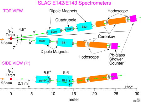
Figure 2: Schematic diagram of SLAC E142/E143 spectrometers

2.2 CERN Experiments

Following the early measurements at SLAC, the EMC (European Muon Collaboration) experiment [57, 58] performed the first measurements at $x<0.1$. Polarized muon beams were produced by pion decay yielding beam intensities of $10^{7}\mu$/s. The small energy loss rate of the muons allowed the use of very thick targets ($\sim$ 1 m) of butanol and methane. The spin structure measurements by EMC came at the end of a series of measurements of unpolarized nucleon and nuclear structure functions, but the impact of the EMC spin measurements was significant. Their low $x$ measurements, accessible due to the high energy of the muons, suggested the breakdown of the naive parton picture that quarks provide essentially all of the spin of the nucleon.

The SMC (Spin Muon Collaboration) experiment [19, 15, 13, 21, 16] began as a dedicated follow-on experiment to the EMC spin measurements using an upgraded apparatus. An extensive program of measurements with polarized ¹H and ²H targets was undertaken over a period of ten years. Improvements in target and beam performance provided high precision data on inclusive spin-dependent structure functions. The large acceptance of the SMC spectrometer in the forward direction (see Fig. 3) allowed them to present the first measurements of spin structure using semi-inclusive hadron production. As with EMC, the high energy of the muon beam provided access to the low $x$ regime ($x<0.01$).

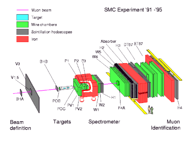
Figure 3: Schematic diagram of SMC spectrometer

A new experiment is underway at CERN whose goal is to provide direct information on the gluon polarization. The COMPASS [111] (COmmon Muon Proton Apparatus for Structure and Spectroscopy) experiment will use a large acceptance spectrometer with full particle identification to generate a high statistics sample of charmed particles. Using targets similar to those used in SMC and an intense muon beam ($\sim 10^{8}\mu$/s) improved measurements of other semi-inclusive asymmetries will also be possible.

2.3 DESY Experiments

Using very thin gaseous targets of pure atoms (¹H, ²H, ³He) and very high currents ($\sim$ 40 mA) of stored, circulating positrons or electrons HERMES (HERa MEasurement of Spin) has been taking data at DESY since 1995. HERMES is a fixed target experiment that uses the stored $e^{\pm}$ beam of the HERA collider. The polarization of the beam is achieved through the Sokolov-Ternov effect [266], whereby the beam becomes transversely polarized due to a small-spin dependence in the synchrotron radiation emission. The transverse polarization is rotated to the longitudinal direction by a spin rotator - a sequence of horizontal and vertical bending magnets that takes advantage of the $g-2$ precession of the $e^{\pm}$. The beam polarization is measured with Compton polarimeters [64].

HERMES has focused its efforts on measurements of semi-inclusive asymmetries, where the scattered $e^{\pm}$ is detected in coincidence with a forward hadron. This was achieved with a large acceptance magnetic spectrometer [11] as shown in Fig. 4. Initial measurements allowed some limited pion identification with a gas threshold Cerenkov detector and a Pb-glass calorimeter. Since 1998 a Ring Imaging Cerenkov (RICH) detector has been in operation allowing full hadron identification over most of the momentum acceptance of the spectrometer.

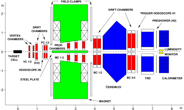
Figure 4: Schematic diagram of HERMES spectrometer

Up to the present, HERMES has taken data only with a longitudinally polarized target. Future runs will focus on high statistics measurements with a transversely polarized target to access eg. transversity (see Sect. 6.1) and $g_{2}$ (see Sect. 6.2).

Promising future spin physics options also exist at DESY if polarized protons can be injected and accelerated in the HERA ring. The HERA-$\vec{\mbox{N}}$ [205] program would use the stored 820 GeV proton beam and a fixed target of gaseous polarized nucleons. This would allow measurements of quark and gluon polarizations at $\sqrt{s}\sim 50$ GeV, complimenting the higher energy measurements possible in the RHIC spin program.

A stored polarized proton beam in HERA would also allow $\vec{e}-\vec{p}$ collider measurements [120] with the existing H1 and ZEUS detectors. Inclusive polarized DIS could be measured to much higher $Q^{2}$ and lower $x$ than existing measurements. This would allow improved extraction of the gluon polarization via the scaling violations of the spin-dependent cross section. Heavy quark and jet production as well as charged-current vs. neutral-current scattering would also allow improved measurements of both quark and gluon polarizations.

2.4 RHIC Spin Program

The Relativistic Heavy-Ion Collider (RHIC) [254] at the Brookhaven National Laboratory recently began operations. This collider was designed to produce high luminosity collisions of high-energy heavy ions as a means to search for a new state of matter known at the quark-gluon plasma. The design of the accelerator also allows the acceleration and collision of high energy beams of polarized protons and a fraction of accelerator operations will be devoted to spin physics with colliding $\vec{p}-\vec{p}$. Beam polarizations of 70% and center-of-mass energies of $\sqrt{s}=50-500$ are expected.

Two large collider detectors, PHENIX [235] and STAR [167], along with several smaller experiments, BRAHMS [276], PHOBOS [273] and PP2PP, will participate in the RHIC spin program. As an example a schematic diagram of the STAR detector is shown in Fig. 5. Longitudinal beam polarization will be available for the PHENIX and STAR detectors enabling measurements of quark and gluon spin distributions (see Sects. 4.2 and 5.74).

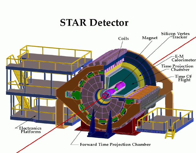
Figure 5: Schematic diagram of the STAR detector

3 Total Quark Helicity Distribution

A large body of data has been accumulated over the past ten years on inclusive polarized lepton scattering from polarized targets. These data allow the extraction of the spin structure functions $g_{1}^{p,n}(x,Q^{2})$ and the nearly model-independent determination of the total quark contribution to the nucleon spin $\Delta\Sigma=(\Delta u+\Delta\bar{u})+(\Delta d+\Delta\bar{d})+(\Delta s+\Delta\bar{s})$. Inclusive data combined with assumptions about flavor symmetry, $SU(3)_{f}$, and results from beta decay provide some model-dependent information on the individual flavor contributions to the nucleon spin. Studies of the $Q^{2}$ dependence of $g_{1}(x,Q^{2})$ allow a first estimate of the gluon spin contribution albeit with fairly large uncertainties. These results are discussed in the following sections.

3.1 Virtual Photon Asymmetries

Virtual photon asymmetries can be defined in terms of a helicity decomposition of the virtual photon-nucleon scattering cross sections. For a transversely polarized virtual photon (eg. with helicity $\pm 1$) incident on a longitudinally polarized nucleon there are two helicity cross sections $\sigma_{1\over 2}$ and $\sigma_{3\over 2}$ and the longitudinal asymmetry is given by

$$A_{1}={\sigma_{1\over 2}-\sigma_{3\over 2}\over\sigma_{1\over 2}+\sigma_{3\over 2}}\ .$$ (27)

$A_{2}$ is a virtual photon asymmetry that results from an interference between transverse and longitudinal virtual photon-nucleon amplitudes:

$$A_{2}={2\sigma_{LT}\over\sigma_{1\over 2}+\sigma_{3\over 2}}\ .$$ (28)

These virtual photon asymmetries, in general a function of $x$ and $Q^{2}$, are related to the nucleon spin structure functions $g_{1}(x,Q^{2})$ and $g_{2}(x,Q^{2})$ via

$$A_{1}(x,Q^{2}) = {g_{1}(x,Q^{2})-\gamma^{2}g_{2}(x,Q^{2})\over F_{1}(x,Q^{2})}\ ,$$

$$A_{2}(x,Q^{2}) = {\gamma\left[g_{1}(x,Q^{2})+g_{2}(x,Q^{2})\right]\over F_{1}(x,Q^{2})}\ ,$$ (29)

where $\gamma=2Mx/\sqrt{Q^{2}}$.

These virtual photon asymmetries can be related to measured lepton asymmetries through polarization and kinematic factors. The experimental longitudinal and transverse lepton asymmetries are defined as

$$A_{||} = {\sigma^{\uparrow\downarrow}-\sigma^{\uparrow\uparrow}\over\sigma^{\uparrow\downarrow}+\sigma^{\uparrow\uparrow}}$$

$$A_{\perp} = {\sigma_{\downarrow\rightarrow}-\sigma_{\uparrow\rightarrow}\over\sigma_{\downarrow\rightarrow}+\sigma_{\uparrow\rightarrow}}\ ,$$ (30)

where $\sigma^{\uparrow\uparrow}$ ($\sigma^{\uparrow\downarrow}$) is the cross section for the lepton and nucleon spins aligned (anti-aligned) longitudinally, while $\sigma_{\downarrow\rightarrow}$ ($\sigma_{\uparrow\rightarrow}$) is the cross section for longitudinally polarized lepton and transversely polarized nucleon. The lepton asymmetries are then given in terms of the virtual photon asymmetries through

$$A_{||} = D\left(A_{1}+\eta A_{2}\right)$$

$$A_{\perp} = d\left(A_{2}-\zeta A_{1}\right)\ .$$ (31)

The virtual photon (de)polarization factor $D$ is approximately equal to $y\equiv\nu/E$ (where $\nu$ is the energy of the virtual photon and $E$ is the lepton energy), but is given explicitly as

$$D=[1-(1-y)\epsilon]/(1+\epsilon R)\ ,$$ (32)

where $\epsilon$ is the magnitude of the virtual photon’s transverse polarization

$$\epsilon=[4(1-y)-\gamma^{2}y^{2}]/[2y^{2}+4(1-y)+\gamma^{2}y^{2}]\ .$$ (33)

and

$$R=\sigma_{L}/\sigma_{T}$$ (34)

is the ratio of longitudinal to transverse virtual photon cross sections.

The other factors are given by

$$\eta=\epsilon\gamma y/[1-\epsilon(1-y)]$$ (35)

$$d=D\sqrt{{2\epsilon\over 1+\epsilon}}$$ (36)

$$\zeta=\eta\left({1+\epsilon\over 2\epsilon}\right)\ .$$ (37)

3.2 Extraction of $g_{1}(x,Q^{2})$

The nucleon structure function is extracted from measurements of the lepton-nucleon longitudinal asymmetry (with longitudinally polarized beam and target)

$$A_{||}={\sigma^{\uparrow\downarrow}-\sigma^{\uparrow\uparrow}\over\sigma^{\uparrow\downarrow}+\sigma^{\uparrow\uparrow}}\ ,$$ (38)

where $\sigma^{\uparrow\uparrow}$ ($\sigma^{\uparrow\downarrow}$) represents the cross section when the electron and nucleon spins are aligned (anti-aligned). These cross sections can also be expressed in terms of spin-independent $\sigma_{U}$ and spin-dependent $\sigma_{P}$ cross sections

$$\sigma^{\uparrow\uparrow}= \sigma_{U}+\sigma_{P}$$ (39)

$$\sigma^{\uparrow\downarrow}= \sigma_{U}-\sigma_{P}\ .$$ (40)

In the limit of stable beam currents, target densities and polarizations, the experimentally measured asymmetry $A_{\rm exp}$ is usually expressed in terms of the measured count rates $N$ and the number of incident electrons $N_{B}$

$$A_{\rm exp}={N^{\uparrow\downarrow}/N_{B}^{\uparrow\downarrow}-N^{\uparrow\uparrow}/N_{B}^{\uparrow\uparrow}\over N^{\uparrow\downarrow}/N_{B}^{\uparrow\downarrow}+N^{\uparrow\uparrow}/N_{B}^{\uparrow\uparrow}}\ .$$ (41)

$A_{||}$ is then determined via

$$A_{||}={A_{\rm exp}\over P_{B}P_{T}f}+\Delta_{\rm RC}\ ,$$ (42)

where $P_{B}$ and $P_{T}$ are the beam and target polarizations respectively, $f$ is a dilution factor due to scattering from unpolarized material and $\Delta_{RC}$ accounts for QED radiative effects [34].

If however there is a time variation of the beam or target polarization or luminosity, the asymmetry should be determined using

$$A_{||}={N^{\uparrow\downarrow}L^{\uparrow\uparrow}-N^{\uparrow\uparrow}L^{\uparrow\downarrow}\over f(N^{\uparrow\downarrow}L^{\uparrow\uparrow}_{P}+N^{\uparrow\uparrow}L^{\uparrow\downarrow}_{P})}+\Delta_{\rm RC}\ ,$$ (43)

since in this case the measured count rates can be written in terms of $\sigma_{U}$ and $\sigma_{P}$

$$\begin{array}[]{rcl}N^{\uparrow\uparrow}=&\sigma_{U}\int n_{B}^{\uparrow\uparrow}(t)dt+\sigma_{P}\int n_{B}^{\uparrow\uparrow}(t)P_{B}(t)P_{T}(t)dt\equiv\sigma_{U}L^{\uparrow\uparrow}+\sigma_{P}L^{\uparrow\uparrow}_{P}\\ N^{\uparrow\downarrow}=&\sigma_{U}\int n_{B}^{\uparrow\downarrow}(t)dt-\sigma_{P}\int n_{B}^{\downarrow\uparrow}(t)P_{B}(t)P_{T}(t)dt\equiv\sigma_{U}L^{\uparrow\downarrow}+\sigma_{P}L^{\uparrow\downarrow}_{P}\ ,\end{array}$$ (44)

where now $n_{B}$ represents the product of beam current and target areal density - the luminosity. In Eq. 44 we have ignored a factor accounting for the acceptance and solid angle of the apparatus which is assumed to be independent of time.

The spin structure function $g_{1}(x,Q^{2})$ can then be determined from the longitudinal asymmetry $A_{||}(x,Q^{2})$,

$$g_{1}={F_{1}\over(1+\gamma^{2})}[A_{||}/D+(\gamma-\eta)A_{2}]\ ,$$ (45)

where $F_{1}\equiv F_{1}(x,Q^{2})$ is the unpolarized structure function. The unpolarized structure function $F_{1}$ is usually determined from measurements of the unpolarized structure function $F_{2}$ and $R$ using

$$F_{1}=F_{2}(1+\gamma^{2})/(2x(1+R))\ .$$ (46)

To use the above equation we need an estimate for $A_{2}$. $|A_{2}|$ is constrained to be less than $\sqrt{R}$ [124], but $A_{2}$ can also be determined from measurements (see Sec. 6.1) with a longitudinally polarized lepton beam and a transversely polarized nucleon target (when combined with the longitudinal asymmetry).

As a guide to the relative importance of various kinematic terms in the above equations we present examples of the magnitude of these terms in Table 2, typical for the SMC and HERMES experiments.

Table 2: Typical kinematic factors entering into the extraction of $g_{1}$. Examples from the SMC and HERMES experiments are given.

SMC
$<x>$	$<Q^{2}>$	$y$	$\gamma$	$\epsilon$	$\gamma-\eta$	$D$
0.005	1.30	0.729	0.008	0.505	0.005	0.721
0.008	2.10	0.736	0.010	0.493	0.006	0.745
0.014	3.60	0.721	0.014	0.517	0.008	0.748
0.025	5.70	0.639	0.020	0.638	0.009	0.671
0.035	7.80	0.625	0.024	0.657	0.011	0.666
0.049	10.40	0.595	0.029	0.695	0.012	0.643
0.077	14.90	0.543	0.037	0.756	0.014	0.592
0.122	21.30	0.490	0.050	0.809	0.016	0.545
0.173	27.80	0.451	0.062	0.843	0.018	0.508
0.242	35.60	0.413	0.076	0.873	0.020	0.468
0.342	45.90	0.376	0.095	0.897	0.022	0.428
0.480	58.00	0.339	0.118	0.919	0.024	0.384
HERMES
$<x>$	$<Q^{2}>$	$y$	$\gamma$	$\epsilon$	$\gamma-\eta$	$D$
0.023	0.92	0.775	0.045	0.427	0.029	0.778
0.033	1.11	0.652	0.059	0.620	0.028	0.635
0.047	1.39	0.573	0.075	0.721	0.030	0.547
0.067	1.73	0.500	0.096	0.798	0.032	0.476
0.095	2.09	0.426	0.123	0.861	0.034	0.405
0.136	2.44	0.348	0.163	0.913	0.035	0.329
0.193	2.81	0.282	0.216	0.945	0.037	0.268
0.274	3.35	0.237	0.281	0.962	0.040	0.227
0.389	4.25	0.212	0.354	0.969	0.047	0.208
0.464	4.80	0.200	0.397	0.972	0.050	0.198
0.550	5.51	0.194	0.440	0.973	0.055	0.195
0.660	7.36	0.216	0.457	0.965	0.065	0.224

For extraction of the neutron structure function $g_{1}^{n}$ from nuclear targets, eg. ²H and ³He, additional corrections must be applied. For the deuteron, the largest contribution is due to the polarized proton in the polarized deuteron which must be subtracted. In addition a D-state admixture into the $p-n$ wave function will reduce the deuteron spin structure function due to the opposite alignment of the $p-n$ spin system in this orbital state; thus

$$g_{1}^{n}(x,Q^{2})={2g_{1}^{d}(x,Q^{2})\over(1-1.5\omega_{D})}-g_{1}^{p}(x,Q^{2})$$ (47)

where $\omega_{D}$ is the D-state probability of the deuteron. Typically a value of $\omega_{D}=0.05\pm 0.01$ [211] is used for this correction.

For polarized ³He, a wavefunction correction for the neutron and proton polarizations is applied using

$$g_{1}^{n}(x,Q^{2})={1\over\rho_{n}}(g_{1}^{{}^{3}He}-2\rho_{p}g_{1}^{p})\ ,$$ (48)

where $\rho_{n}=(86\pm 2)\%$ and $\rho_{p}=(-2.8\pm 0.4)\%$ as taken from a number of calculations [146, 106]. Additional corrections due to the neutron binding energy and Fermi motion have also been investigated [75, 106, 260] and shown to be relatively small.

3.3 Recent Results for $g_{1}(x,Q^{2})$

Most of the experiments listed in Table 1 have contributed high precision data on the spin structure function $g_{1}(x,Q^{2})$. Where there is overlap (in $x$ and $Q^{2}$), the agreement between the experiments is extremely good. This can be seen in Fig. 6, where the ratio of the polarized to unpolarized proton structure function $g_{1}^{p}/F_{1}^{p}$ is shown. Analysis of the $Q^{2}$ dependence of this ratio [4] has shown that it is consistent experimentally with being independent of $Q^{2}$ within the range of existing experiments, although this behavior is not expected to persist for all $Q^{2}$.

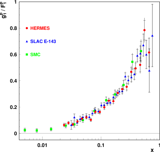
Figure 6: Ratio of polarized to unpolarized proton structure function from the SMC, E143 and HERMES experiments.

A comparison of the spin structure functions $g_{1}^{p,d,n}$ are shown in Fig. 7. Some residual $Q^{2}$ dependence is visible in the comparison of the SMC data with the other experiments. The general $Q^{2}$ dependence of $g_{1}$ will be discussed in Sect. 3.5.

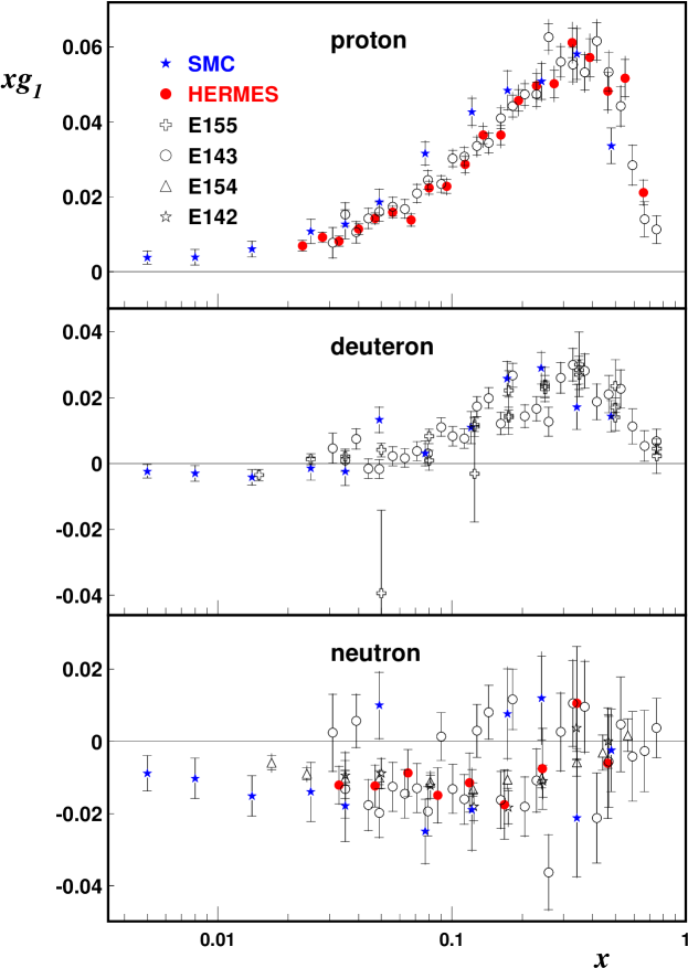
Figure 7: Compilation of the world’s data on $g_{1}^{p},g_{1}^{d},g_{1}^{n}$

While the results shown in Figs. 6,7 correspond to $Q^{2}>1$ GeV², data also exists at lower $Q^{2}$, because of the large kinematic acceptance in many of the experiments. Much of this data [4, 25, 238], when expressed as $g_{1}/F_{1}$ appears to be largely independent of $Q^{2}$.

3.4 First Moments of $g_{1}(x,Q^{2})$

The initial interest in measurements of $g_{1}(x,Q^{2})$ was in comparing the measurements to several predicted sum rules, specifically the Ellis-Jaffe and Bjorken sum rules. These sum rules relate integrals over the measured structure functions to measurements of neutron and hyperon beta-decay.

The Ellis-Jaffe sum rule [137] starts with the leading-order QPM result for the integral of $g_{1}(x)$:

$$\int_{0}^{1}g_{1}(x)dx={1\over 2}\int_{0}^{1}\sum_{i}e^{2}_{i}\Delta q_{i}(x)dx\ ,$$ (49)

where the sum is over $u,d,s,\bar{u},\bar{d},\bar{s}$ for three active quark flavors and the $Q^{2}$ dependence has been suppressed as it is absent in the simple QPM. Introducing the $SU(3)_{f}$ nucleon axial charges:

$$a_{0}= (\Delta u+\Delta\bar{u})+(\Delta d+\Delta\bar{d})+(\Delta s+\Delta\bar{s})$$ (50)

$$a_{3}= (\Delta u+\Delta\bar{u})-(\Delta d\ +\Delta\bar{d})$$ (51)

$$a_{8}= (\Delta u+\Delta\bar{u})+(\Delta d+\Delta\bar{d})-2(\Delta s+\Delta\bar{s})\ ,$$ (52)

where $\Delta q_{i}=\int_{0}^{1}\Delta q_{i}(x)dx$, the Ellis-Jaffe sum rule then assumes that the strange quark and sea polarizations are zero ($\Delta s=\Delta\bar{q}_{i}=0$). Then for the proton and neutron integrals the Ellis-Jaffe sum rule gives:

$$\Gamma_{1}^{p}\equiv\int_{0}^{1}g_{1}^{p}(x)= {3\over 36}a_{3}+{1\over 36}a_{8}+{4\over 36}a_{0}=0.186\pm 0.004$$

$$\Gamma_{1}^{n}\equiv\int_{0}^{1}g_{1}^{p}(x)= -{3\over 36}a_{3}+{1\over 36}a_{8}+{4\over 36}a_{0}=-0.025\pm 0.004\ .$$ (53)

To evaluate the integrals it is assumed that $a_{0}=a_{8}$ which is true if $\Delta s=0$. Then $a_{3}$ is determined from the ratio of axial-vector to vector coupling constants in neutron decay $a_{3}=-g_{A}/g_{V}=1.2670\pm 0.0035$ [241]. A value for $a_{8}$ can be estimated with the additional assumption of SU(3) flavor symmetry which allows one to express $g_{A}/g_{V}$ for hyperon beta decays in terms of $a_{3}$ and $a_{8}$ (see Table 3), giving $a_{8}=0.58\pm 0.03$. Nucleon and hyperon beta decay is sometimes parameterized in terms of the $F$ and $D$ coefficients. These coefficients are related to the axial charges $a_{3}$ and $a_{8}$ with

$$a_{3} = F+D$$

$$a_{8} = 3F-D\ .$$ (54)

Table 3: Relation of the neutron and hyperon beta decays to the nucleon’s axial charges (as defined in the text) assuming $SU(3)_{f}$ symmetry.

Decay	$g_{A}/g_{V}$ in terms of Axial charges	Experimental [241]
$n\rightarrow pe_{-}\bar{\nu}_{e}$	$-a_{3}$	$-1.2670\pm 0.0035$
$\Lambda\rightarrow pe^{-}\bar{\nu}_{e}$	$-{1\over 2}a_{3}-{1\over 6}a_{8}$	$-0.718\pm 0.015$
$\Sigma^{-}\rightarrow ne^{-}\bar{\nu}_{e}$	${1\over 2}a_{3}-{1\over 2}a_{8}$	$0.340\pm 0.017$
$\Xi^{-}\rightarrow\Lambda e^{-}\bar{\nu}_{e}$	$-{1\over 3}a_{8}$	$-0.25\pm 0.05$

The assumptions implicit in the Ellis-Jaffe sum rule, eg. $\Delta s=\Delta\bar{q}_{i}=0$ and $SU(3)_{f}$ symmetry, may be significantly violated. On the contrary, the Bjorken sum rule [74]

$$\int_{0}^{1}\left[g_{1}^{p}(x)-g_{1}^{n}(x)\right]dx={1\over 6}a_{3}=0.211\pm 0.001$$ (55)

requires only current algebra and isospin symmetry (eg. $\Delta u^{p}=\Delta d^{n}$) in its derivation. Note that both the Ellis-Jaffe and Bjorken sum rules must be corrected for QCD radiative corrections. For example, these corrections have been evaluated up to order $\alpha_{s}^{3}$  [217] and amount to $\sim 10\%$ correction for the Ellis-Jaffe sum rule and $\sim 15\%$ correction for the Bjorken sum rule at $Q^{2}=5$ GeV².

Comparison of these predictions with experiment requires forming the integrals of the measurements of $g_{1}(x,Q^{2})$ over the full $x$ range from $0\rightarrow 1$ at a fixed $Q^{2}$. Thus extrapolations are necessary in order to include regions of unmeasured $x$, both at high and low $x$. For the large $x$ region this is straightforward: since $g_{1}(x)$ is proportional to a difference of quark distributions it must approach zero as $x\rightarrow 1$ as this is the observed behavior of the unpolarized distributions. However the low $x$ region is problematic, as there is no clear dependence expected. In the first analyses simple extrapolations based on Regge parameterizations [170, 135] were used. Thus $g_{1}(x)$ was assumed to be nearly constant for $x\rightarrow 0$. Later, Next-to-Leading-Order (NLO) QCD calculations [136] (see Sec. 3.5) suggested that these parameterizations likely underestimated the low $x$ contributions. The NLO calculations cannot predict the actual $x$ dependence of the structure function, but can only take a given $x$ dependence and predict its dependence on $Q^{2}$. Thus by using the Regge parameterizations for low $Q^{2}\mathrel{\raise 1.29167pt\hbox{$<$}\mkern-14.0mu\lower 2.58334pt\hbox{$\sim$}}1$, they can give the low $x$ behavior at the $Q^{2}$ of the experiments, eg. $Q^{2}\sim 3-10$ GeV².

Evaluating the experimental integrals at a fixed $Q^{2}$ requires an extrapolation of the measured structure function. In general, for each experiment, the experimental acceptance imposes a correlation between $x$ and $Q^{2}$ preventing a single experiment from measuring the full range in $x$ at a constant value of $Q^{2}$. Thus the data must be QCD-evolved to a fixed value of $Q^{2}$. This has often been done by exploiting the observed $Q^{2}$ independence of $g_{1}(x,Q^{2})/F_{1}(x,Q^{2})$ (see Fig. 6). In this case most of the $Q^{2}$ dependence of $g_{1}(x,Q^{2})$ results from the $Q^{2}$ dependence of the unpolarized structure function $F_{1}(x,Q^{2})$ which is well measured in other experiments. Alternatively, NLO QCD fits (as described in the next section) can be used to evolve the data sets to a common $Q^{2}$.

The E155 collaboration has recently reported [49] a global analysis of spin structure function integrals. They have evolved the world data set on $g_{1}^{p}(x,Q^{2})$ and $g_{1}^{n}(x,Q^{2})$ to $Q^{2}=5$ GeV² and have extrapolated to low and to high $x$ using a NLO fit to the data. Their results are compared in Table 4 with the predictions for the Ellis-Jaffe and Bjorken sum rules (Eqs. 53,55) including QCD radiative corrections for $Q^{2}=5$ GeV² up to order $\alpha_{s}^{3}$ using the calculations of Ref. [217] and world-average for $\alpha_{s}$ [241].

Table 4: Comparison of Sum Rule predictions including corrections up to order $\alpha_{s}^{3}$ with a global analysis of the experiments.

Sum Rule	Calculation	Experiment [49]
EJ Sum $\Gamma_{1}^{p}(Q^{2}=5$ GeV2)	$0.163\pm 0.004$	$0.118\pm 0.004\pm 0.007$
EJ Sum $\Gamma_{1}^{n}(Q^{2}=5$ GeV2)	$-0.019\pm 0.004$	$-0.058\pm 0.005\pm 0.008$
Bj $\Gamma_{1}^{p}-\Gamma_{1}^{n}(Q^{2}=5$ GeV2)	$0.181\pm 0.005$	$0.176\pm 0.003\pm 0.007$

As seen in Table 4 the Bjorken sum rule is well verified. In fact some analyses [136] have assumed the validity of the Bjorken sum rule and used the $Q^{2}$ dependence of $\Gamma_{1}^{p}-\Gamma_{1}^{n}$ to extract a useful value for $\alpha_{s}$. In contrast there is a strong violation of the Ellis-Jaffe sum rules. Many early analyses of these results interpreted the violation in terms of a non-zero value for $\Delta s$ (in which case $a_{0}\neq a_{8}$), using only the leading order QPM. However modern analyses have demonstrated that a full NLO analysis is necessary in order to interpret the results. This analysis will be described in the next section. Here, for completeness, we give the leading order QPM result.

Within the leading order QPM, $\Delta u+\Delta\bar{u},\Delta d+\Delta\bar{d}$ and $\Delta s+\Delta\bar{s}$ can be determined by using Eqs. 53 with the experimental values from Table 4. Dropping the assumption of $a_{0}=a_{8}$, but retaining the $SU(3)_{f}$ assumption to determine $a_{8}$, one finds:

$$\Delta u+\Delta\bar{u}=0.78\pm 0.03,\,\,\,\Delta d+\Delta\bar{d}=-0.48\pm 0.03,\,\,\,\Delta s+\Delta\bar{s}=-0.14\pm 0.03$$ (56)

after applying the relevant QCD radiative corrections to the terms in Eq. 53 (corresponding to a factor of 0.859 multiplying the triplet $a_{3}$ and octet $a_{8}$ charges and a factor of 0.878 multiplying the singlet $a_{0}$ charge for $Q^{2}=5$ GeV²). This then gives a very small value for the total quark contribution to the nucleon’s spin, $\Delta\Sigma=0.16\pm 0.08$. Note that the quoted uncertainties reflect only the uncertainty in the measured value of $\Gamma_{1}$ and not possible systematic effects due to the assumption of $SU(3)_{f}$ symmetry and NLO effects. Studies of the effect of $SU(3)_{f}$ symmetry violations have been estimated [9] to have little effect on the uncertainty in $\Delta u$ and $\Delta d$, but can increase the uncertainty on $\Delta s$ by a factor of two to three. NLO effects are the subject of the next section.

3.5 Next-to-Leading Order Evolution of $g_{1}(x,Q^{2})$

As discussed above the spin structure functions possess a significant $Q^{2}$ dependence due to QCD radiative effects. It is important to understand these effects for a number of reasons, including comparison of different experiments, forming structure function integrals, parameterizing the data and obtaining sensitivity to the gluon spin distribution. As the experiments are taken at different accelerator facilities with differing beam energies the data span a range of $Q^{2}$. In addition, because of the extensive data set that has been accumulated and the recently computed higher-order QCD corrections, it is possible to produce parameterizations of the data based on Next-to-Leading-Order (NLO) QCD fits to the data. This provides important input to future experiments utilizing polarized beams (eg. the RHIC spin program). These fits have also yielded some initial information on the gluon spin distribution, because of the radiative effects that couple the quark and gluon spin distributions at NLO.

At NLO the QPM expression for the spin structure function becomes

$$g_{1}(x,Q^{2})={1\over 2}\sum_{i}e_{i}^{2}C_{q}(x,\alpha_{s})\otimes\Delta q_{i}(x,Q^{2})+{1\over N_{f}}C_{g}(x,\alpha_{s})\otimes\Delta G(x,Q^{2})\ ,$$ (57)

where for three active quark flavors ($N_{f}=3$) the sum is again over quarks and antiquarks: $u,d,s,\bar{u},\bar{d},\bar{s}$. $C_{q}(x,\alpha_{s})$ and $C_{g}(x,\alpha_{s})$ are Wilson coefficients and correspond to the polarized photon-quark and photon-gluon hard scattering cross section respectively. The convolution $\otimes$ is defined as

$$C(x,\alpha_{s})\otimes q(x,Q^{2})=\int_{x}^{1}{dy\over y}C({x\over y},\alpha_{S})q(x,Q^{2})\ .$$ (58)

The explicit dependence of the nucleon spin structure function on the gluon spin distribution is apparent in Eq. 57. At Leading Order (LO) $C_{q}^{0}=\delta(1-x)$ and $C_{g}^{0}=0$ and the usual dependence (Eq. 49) of the spin structure function on the quark spin distributions emerges. At NLO however, the factorization between the quark spin distributions and coefficient functions shown in Eq. 57 cannot be defined unambiguously. This is known as factorization scheme dependence and results from an ambiguity in how the perturbative physics is divided between the definition of the quark/gluon spin distributions and the coefficient functions. There are also ambiguities associated with the definition of the $\gamma_{5}$ matrix in $n$ dimensions [272] and in how to include the axial anomaly. This has lead to a variety of factorization schemes that deal with these ambiguities by different means.

We can classify the factorization schemes in terms of their treatment of the higher order terms in the expansion of the coefficient functions. The $Q^{2}$ dependence of this expansion can be written as:

$$C_{i}(x,\alpha_{s})=C_{i}^{0}(x)+{\alpha_{s}(Q^{2})\over 2\pi}C_{i}^{(1)}+\cdots\ .$$ (59)

In the so-called Modified-Minimal-Subtraction ($\overline{\rm MS}$) scheme [231, 277] the first moment of the NLO correction to $C_{g}$ vanishes (i.e. $\int_{0}^{1}C_{g}^{(1)}(x)dx=0$), such that $\Delta G$ does not contribute to the first moment of $g_{1}$. In the Adler-Bardeen [63, 38] scheme (AB) the treatment of the axial anomaly causes the first moment of $C_{g}^{(1)}$ to be non-zero, leading to a dependence of $\int g_{1}(x)dx$ on $\int\Delta G(x)dx$. This then leads to a difference in the singlet quark distribution $\Delta\Sigma$ in the two schemes:

$$\Delta\Sigma(x,Q^{2})_{\rm AB} = \Delta\Sigma(x,Q^{2})_{\overline{\rm MS}}+N_{f}{\alpha_{s}(Q^{2})\over 2\pi}\int_{x}^{1}{dy\over y}\Delta G(y,Q^{2})$$

$$\Delta G(x,Q^{2})_{\rm AB} = \Delta G(x,Q^{2})_{\overline{\rm MS}}\ .$$ (60)

A third scheme, sometimes called the JET scheme [101, 218] or chirally invariant (CI) scheme [104], is also used. This scheme attempts to include all perturbative anomaly effects into $C_{g}$. Of course any physical observables (eg. $g_{1}(x,Q^{2})$) are independent of the choice of scheme. There are also straightforward transformations [38, 237, 219] that relate the schemes and their results to one another.

Once a choice of scheme is made the $Q^{2}$ dependence of $g_{1}$ can be calculated using the Dokahitzer-Gribov-Lipatov-Altarelli-Parisi (DGLAP) [163] equations. These equations characterize the evolution of the spin distributions in terms of $Q^{2}$-dependent splitting functions $P_{ij}(x,\alpha_{s})$:

$${d\over d\ln Q^{2}}\Delta q_{NS}(x,Q^{2}) = {\alpha_{s}(Q^{2})\over 2\pi}P_{qq}^{NS}\otimes\Delta q_{NS}$$

$${d\over d\ln Q^{2}}\left(\begin{array}[]{c}\Delta\Sigma\\ \Delta G\end{array}\right) = {\alpha_{s}(Q^{2})\over 2\pi}\left(\begin{array}[]{cc}P_{qq}&P_{qg}\\ P_{gq}&P_{gg}\end{array}\right)\otimes\left(\begin{array}[]{c}\Delta\Sigma\\ \Delta G\end{array}\right)\ ,$$ (67)

where the non-singlet quark distributions $\Delta q_{NS}(x,Q^{2})$ for three quark flavors are defined with

$$\Delta q_{NS}(x,Q^{2})=(\Delta u+\Delta\bar{u})-{1\over 2}(\Delta d+\Delta\bar{d})-{1\over 2}(\Delta s+\Delta\bar{s})\ .$$ (68)

The splitting functions $P_{ij}$ can be expanded in a form similar to that for the coefficient functions $C_{i}(x,\alpha_{s})$ in Eq. 59 and have been recently evaluated [231, 277] in NLO.

The remaining ingredients in providing a fit to the data are the choice of starting momentum scale $Q_{0}^{2}$ and the form of the parton distributions at this $Q_{0}^{2}$. The momentum scale is usually chosen to be $\leq 1$ GeV² so that the quark spin distributions are dominated by the valence quarks and the gluon spin distribution is likely to be small. Also, as discussed above, at lower momentum transfer some models for the $x$ dependence of the distributions (eg. Regge-type models for the low $x$ region) are more reliable. The form of the polarized parton distributions at the starting momentum scale are parameterized by a variety of $x$ dependences with various powers. This parameterization is the source of some of the largest uncertainties as the $x$ dependence at low values of $x\leq 0.003$ is largely unconstrained by the measurements. As an example, Ref. [38] assumes for one of its fits that the polarized parton distributions can be parameterized by

$$\Delta q_{i}(x,Q^{2}_{0})=A_{i}x^{\alpha_{i}}\left(1-x\right)^{\beta_{i}}\left(1+\gamma_{i}x^{\delta_{i}}\right)\ .$$ (69)

With such a large number of parameters it is usually required to place additional constraints on some of the parameters. Often $SU(3)_{f}$ symmetry is used to constrain the parameters, or the positivity of the distributions ($|\Delta q_{i}(x)|\leq q_{i}(x)$) is enforced (note that this positivity is strictly valid only when all orders are included; see Ref. [39]). Thus in other fits, the polarized distributions are taken to be proportional to the unpolarized distributions as in eg. Ref. [49]:

$$\Delta q_{i}(x,Q^{2}_{0})=A_{i}x^{\alpha_{i}}q_{i}(x,Q^{2}_{0})\ .$$ (70)

A large number of NLO fits have recently been published [156, 151, 63, 38, 24, 8, 86, 162, 219, 220, 221, 161, 49, 115]. These fits include a wide variety of assumptions for the forms of the polarized parton distributions, differences in factorization scheme and what data sets they include in the fit (only the most recent fits [161] include all the published inclusive data). Some fits [115] have even performed a NLO analysis including information from semi-inclusive scattering (see Sec. 4.1). A comparison of the results from some of these recent fits is shown in Table 5.

Table 5: Results from NLO fits to data for first moments of quark and gluon distributions. Missing data refers to data sets that are not included in the fits, PPDF refers to the assumptions for Polarized Parton Distribution Functions and $Q^{2}_{ev}$ refers to the evolved $Q^{2}$ where the first moments are evaluated.

Reference	Scheme	$Q^{2}_{0}$	Missing Data	PPDF	$Q^{2}_{ev}$	$\Delta\Sigma$	$\Delta G$
		GeV2			GeV2
ABFR98 [38]	AB	1	HERMES(p)	$\Delta q_{i}\not\propto q_{i}$	1	$0.41\pm 0.03$	$0.95\pm 0.18$
(Fit-A)			E155(pd)
			Semi-inc
LSS99 [221]	JET	1	Semi-inc	$\Delta q_{i}\propto q_{i}$	1	$0.39\pm 0.04$	$0.57\pm 0.14$
	AB	1				$0.41\pm 0.04$	$0.58\pm 0.04$
	$\overline{\rm MS}$	1				$0.28\pm 0.04$	$0.07\pm 0.10$
GOTO00 [161]	$\overline{\rm MS}$	1	Semi-inc	$\Delta q_{i}\propto q_{i}$	1	0.050	0.53
(NLO-1)		1			5	0.054	0.86
		1			10	0.055	1.0
FS00 [115]	$\overline{\rm MS}$	0.5	–	$\Delta q_{i}\propto q_{i}$	10	0.050	0.53
(ii)

Note that in the JET and AB schemes $\Delta\Sigma$ includes a contribution from $\Delta G$. Thus the overriding result of these fits is that the quark spin distribution $\Delta\Sigma$ is constrained between $0.05-0.30$ but that the gluon distribution and its first moment are largely unconstrained. The extracted value for $\Delta G(Q^{2}=5\,{\rm GeV}^{2})$ is typically positive but the corresponding uncertainty is often $50-100\%$ of the value. Note that the uncertainties listed in Table 5 are dependent on the assumptions used in the fits.

Estimates of the contribution from higher twist effects [62, 198] ($1/Q^{2}$ corrections) suggest that the effects are relatively small at the present experimental $Q^{2}$. This is further supported by the generally good fits that the NLO QCD calculations can achieve without including possible higher-twist effects.

Lattice QCD calculations of the first moments and second moments of the polarized spin distributions are underway [150, 125, 158, 165]. Agreement with NLO fits to the data is reasonable for the quark contribution, although the Lattice calculations are not yet able to calculate the gluon contribution.

4 Individual Quark Helicity Distributions

As shown in the last section, the inclusive lepton asymmetries generally provide spin structure information only for the sum over quark flavors. Access to the individual flavor contributions to the nucleon spin requires assumptions including $SU(3)_{f}$ symmetry in the weak decay of the octet baryons (nucleons and strange hyperons).

Potentially more direct information on the individual contributions of $u,d$, and $s$ quarks as well as the separate contributions of valence and sea quarks is possible via semi-inclusive scattering. Here one or more hadrons in coincidence with the scattered lepton are detected. The charge of the hadron and its valence quark composition provide sensitivity to the flavor of the struck quark within the Quark-Parton Model (QPM).

Semi-inclusive asymmetries also allow access to the third leading-order quark distribution $\delta q$ called transversity. Because of the chiral odd structure of this distribution function it is not measurable in inclusive DIS. Transversity will be discussed in Sec. 6.2. Additionally, semi-inclusive asymmetries can provide a degree of selectivity for different reaction mechanisms that are sensitive to the gluon polarization. The sensitivity of semi-inclusive asymmetries to the gluon polarization will be discussed in Sect. 5. The flavor decomposition of the nucleon spin using semi-inclusive scattering will be discussed in the next two sections.

4.1 Semi-Inclusive Polarized Lepton Scattering

Within the QPM, the cross section for leptoproduction of a hadron (semi-inclusive scattering) can be expressed as

$${d\sigma^{h}\over dz}=\sigma_{DIS}(x,Q^{2})\left[{\sum_{i}e_{i}^{2}q_{i}(x,Q^{2})D_{i}^{h}(z,Q^{2})\over\sum_{i}e_{i}^{2}q_{i}(x,Q^{2})}\right]\ ,$$ (71)

where $\sigma_{DIS}$ is the inclusive DIS cross section, the fragmentation function, $D_{i}^{h}(z,Q^{2})$, is the probability that the hadron $h$ originated from the struck quark of flavor $i$, $z=E_{h}/\nu$ is the hadron momentum fraction and the sums are over quark and antiquark flavors $u,d,s,\bar{u},\bar{d},\bar{s}$. To maximize the sensitivity to the struck “current” quark, kinematic cuts are imposed on the data in order to suppress effects from target fragmentation. These cuts typically correspond to $W^{2}>9-10$ GeV² and $z>0.2$.

In general the fragmentation functions $D_{i}^{h}(z,Q^{2})$ depend on both the quark flavor and the hadron type. In particular for a given hadron $D_{i}^{h}\neq D_{j}^{h}$. This effect can be understood in terms of the QPM: if the struck quark is a valence quark for a particular hadron, it is more likely to fragment into that hadron (eg. $D_{u}^{\pi^{+}}>D_{d}^{\pi^{+}}$). A flavor sensitivity is therefore obtained as is a sensitivity to the antiquarks (eg. $D_{\bar{d}}^{\pi^{+}}>D_{d}^{\pi^{+}}$).

Eq. 71 displays a factorization of the cross section into separate $z$ and $x$ dependent terms. This is an assumption of the QPM and must be experimentally tested. Measurements of unpolarized hadron leptoproduction [53] have shown good agreement with the factorization hypothesis. Data from $e^{+}-e^{-}\rightarrow$ hadrons can also be used to extract fragmentation functions [209]. Both the $Q^{2}$ and $z$ dependence of the fragmentation functions have been parameterized within string models of fragmentation [263] that are in reasonable agreement with the measurements. Recently the $Q^{2}$ dependence of the fragmentation functions have been calculated to NLO [73].

Assuming factorization of the cross section as given in Eq. 71, we can write the asymmetry for leptoproduction of a hadron as

$$A_{1}^{h}(x,Q^{2})={\sum_{i}e_{i}^{2}\Delta q_{i}(x,Q^{2})\int_{z}D_{q}^{h}(z,Q^{2})dz\over\sum_{i}e_{i}^{2}q_{i}(x,Q^{2})\int_{z}D_{i}^{h}(z,Q^{2})dz}\ .$$ (72)

Due to parity conservation the fragmentation functions contain no spin dependence as long as the final-state polarization of the hadron is not measured (spin dependent fragmentation can be accessed through the self-analyzing decay of $\Lambda$ - see Sec. 8.2). By making measurements with $H,D$ and ³He targets for different final-state hadrons and assuming isospin symmetry of the quark distributions and fragmentation functions a system of linear equations can be constructed:

$$\left(\begin{array}[]{c}A_{\pi^{+}}^{p}\\ A_{\pi^{-}}^{p}\\ A_{K^{+}}^{n}\\ A_{K^{+}}^{n}\\ \vdots\end{array}\right)=f[q_{i}(x),D_{i}^{h}]\left(\begin{array}[]{c}\Delta u\\ \Delta d\\ \Delta s\\ \Delta\bar{u}\\ \vdots\end{array}\right)$$ (73)

and solved for the $\Delta q_{i}$. In these equations, the unpolarized quark distributions are taken from a variety of parameterizations (eg. Ref. [157, 214]) and the fragmentation functions are taken from measurements [53, 209] or parameterizations [263].

EMC, SMC and HERMES have made measurements of semi-inclusive asymmetries. A comparison of the measurements from SMC and HERMES is shown in Fig. 8. As the HERMES data are taken at $<Q^{2}>=2.5$ GeV² and the SMC data at $<Q^{2}>=10$ GeV², these data suggest that the semi-inclusive asymmetries are also approximately independent of $Q^{2}$.

Figure 8: Virtual photon asymmetries for semi-inclusive lepton scattering. Inclusive asymmetries are shown in the leftmost panels for comparison.

It is important to note, especially for the lower $Q^{2}$ data of HERMES, that Eq. 72 must be modified if parameterizations of the unpolarized quark distributions are used. In some parameterizations it is assumed that the unpolarized structure functions are related by the Callen-Gross approximation $F_{1}=F_{2}/2x$ rather than by the complete expression $F_{1}=F_{2}(1+\gamma^{2})/(2x(1+R))$. Thus some experimental groups will present Eq. 72 with an extra factor of $(1+R)/(1+\gamma^{2})$ included.

Up to now results have only been reported for positively and negatively charged hadrons (summing over $\pi$, $p$ and $K$) because of the lack of sufficient particle identification in the experiments. This reduces the sensitivity to some quark flavors (eg. strangeness) and requires additional assumptions about the flavor dependence of the sea quark and anti-quark distributions. Two assumptions have been used to extract information on the flavor and sea dependence of the quark polarizations, namely

$${\Delta u_{s}(x)\over u_{s}(x)}={\Delta d_{s}(x)\over d_{s}(x)}={\Delta s(x)\over s(x)}={\Delta\bar{u}(x)\over\bar{u}(x)}={\Delta\bar{d}(x)\over\bar{d}(x)}={\Delta\bar{s}(x)\over\bar{s}(x)}$$ (74)

or

$$\Delta u_{s}(x)=\Delta d_{s}(x)=\Delta s(x)=\Delta\bar{u}(x)=\Delta\bar{d}(x)=\Delta\bar{s}(x)\ .$$ (75)

Here $\Delta u_{s}$ and $\Delta d_{s}$ represent the $u$ and $d$ sea quark spin distributions. A comparison of the extracted valence and sea quark distributions from HERMES and SMC is shown in Fig. 9. The valence distributions are defined using $\Delta q_{v}=\Delta q-\Delta\bar{q}$. Typical systematic errors are also shown in Fig. 9 and include the difference due to the two assumptions for the sea distributions given by Eqs. 74- 75. The solid lines are positivity limits corresponding to $\Delta q(x)=q(x)$. The dashed lines are parameterizations from Gehrmann and Stirling (Gluon A-LO) [151].

Figure 9: Quark flavor spin structure from hadron leptoproduction from the HERMES [12] and SMC [20, 23] experiments. Both data sets have been evolved to $<Q^{2}>=2.5$ GeV². Typical systematic errors from Ref. [12] are shown in the shaded band. The solid lines are the positivity limits corresponding to $\Delta q(x)=q(x)$. The dashed lines are the parameterization from Gehrmann and Stirling (Gluon A-LO) [151].

Values for the integrals over the spin distributions from SMC and HERMES are compared in Table 6. The dominant sensitivity to $\Delta\bar{u}$ within the quark sea is due to the factor of two larger charge compared to $\bar{d}$ and $\bar{s}$.

Table 6: Comparison of the first moment of separated quark spin distributions as determined from semi-inclusive DIS lepton scattering. Both statistical and systematic uncertainties are given.

$\int_{0}^{1}\Delta q_{i}(x)dx$	SMC results	HERMES results
	$Q^{2}=10$ GeV2	$Q^{2}=2.5$ GeV2
$\Delta u_{v}$	$~{}~{}~{}0.77\pm 0.10\pm 0.08$	$~{}~{}~{}0.57\pm 0.05\pm 0.08$
$\Delta d_{v}$	$-0.52\pm 0.14\pm 0.09$	$-0.22\pm 0.11\pm 0.13$
$\Delta\bar{u}$	$~{}~{}~{}0.01\pm 0.04\pm 0.03$	$-0.01\pm 0.02\pm 0.03$

While the experimental results presented in Table 6 have been extracted through a Leading-Order QCD analysis, NLO analyses are possible [114] and several such analyses have recently been published [115].

Future measurements from HERMES and COMPASS will include full particle identification providing greater sensitivity to the flavor separation of the quark spin distributions. In particular, due to the presence of strange quarks in the $K$ valence quark distribution, $K$ identification is expected to give significant sensitity to $\Delta s(x)$.

4.2 High Energy $\vec{p}-p$ Collisions

The production of weak $W^{\pm}$ bosons in high energy $\vec{p}-p$ collisions at RHIC provides unique sensitivity to the quark and antiquark spin distributions. The maximal parity violation in the interaction and the dependence of the production on the weak charge of the quarks can be used in principle to select specific flavor and charge for the quarks. Thus the single spin longitudinal asymmetry for $W^{+}$ production ($\vec{p}p\rightarrow W^{+}X$) can be written [85]

Figure 10: W boson production in $\vec{p}p$ collisions.

$$A_{L}={\Delta u(x_{1})\bar{d}(x_{2})-\Delta\bar{d}(x_{1})u(x_{2})\over u(x_{1})\bar{d}(x_{2})+\bar{d}(x_{1})u(x_{2})}\ ,$$ (76)

where $x_{1}$ and $x_{2}$ refer to the $x$ value of the quark and antiquark participating in the interaction (see for example Fig. 10). Making the replacement $u\leftrightarrow d$ gives the asymmetry for $W^{-}$ production. In the experiments the $W^{\pm}$ are detected through their decay to a charged lepton ($\mu^{\pm}$ in PHENIX and $e^{\pm}$ in STAR) and the $x_{1},x_{2}$ values are determined from the angles and energies of those detected leptons. Thus for $W^{+}$ production with $x_{1}\gg x_{2}$ the valence quarks are selected for $x_{1}$ and $A_{L}(W^{+})\sim\Delta u(x_{1})/u(x_{1})$, while for $x_{1}\ll x_{2}$ valence quarks are selected for $x_{2}$ and $A_{L}(W^{+})\sim\Delta\bar{d}(x_{1})/\bar{d}(x_{1})$. Detection of $W^{-}$ then gives $\Delta\bar{u}/\bar{u}$ and $\Delta d/d$. An example of the expected sensitivity of the PHENIX experiment after about four years of data taking is shown in Fig. 11.

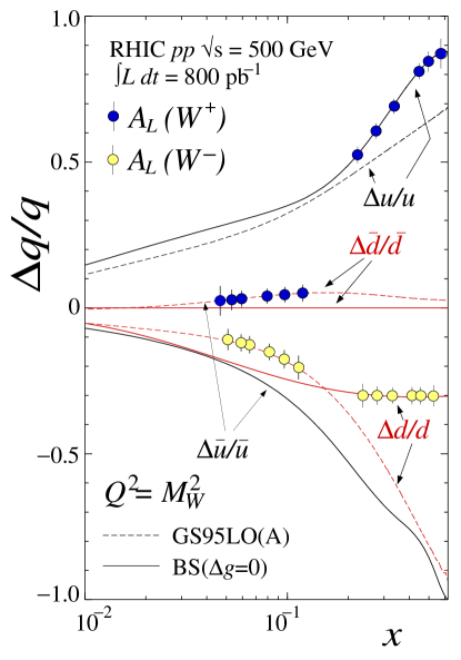
Figure 11: Predicted sensitivity of the PHENIX detector at RHIC for measurement of the quark flavor spin contributions.

5 Gluon Helicity Distribution

As remarked in the Introduction, the gluon contribution to the spin of the nucleon can be separated into spin and orbital parts. As with its unpolarized counterpart, the polarized gluon distribution is difficult to access experimentally. There exists no theoretically clean and, at the same time, experimentally straightforward hard scattering process to directly measure the distribution. In the last decade, many interesting ideas have been proposed and some have led to useful initial results from the present generation of experiments; others will be tested soon at various facilities around the world.

In the following subsections, we discuss a few representative hard-scattering processes in which the gluon spin distribution can be measured.

Figure 12: Typical gluon helicity distributions [151] obtained from fits to available polarized DIS data.

5.1 $\Delta G(x)$ from QCD Scale Evolution

As discussed in Section 3.5, the polarized gluon distribution enters in the factorization formula for spin-dependent inclusive deep-inelastic scattering. Since the $g_{1}(x,Q^{2})$ structure function involves both the singlet quark and gluon distributions as shown in Eq. 57, only the $Q^{2}$ dependence of the data can be exploited to separate them. The $Q^{2}$ dependence results from two different sources: the running coupling $\alpha_{s}(Q^{2})$ in the coefficient functions and the scale evolution of the parton distributions. As the gluon contribution has its own characteristic $Q^{2}$ behavior, it can be isolated in principle from data taken over a wide range of $Q^{2}$.

Because the currently available experimental data have rather limited $Q^{2}$ coverage, there presently is a large uncertainty in extracting the polarized gluon distribution. As described in Sec. 3.5, a number of NLO fits to the world data have been performed to extract the polarized parton densities. While the results for the polarized quark densities are relatively stable, the extracted polarized gluon distribution depends strongly on the assumptions made about the $x$-dependence of the initial parameterization. Different fits produce results at a fixed $x$ differing by an order of magnitude and even the sign is not well constrained.

Several sets of polarized gluon distributions have been used widely in the literature for the purpose of estimating outcomes for future experiments. An example from Ref. [151] of the range of possible distributions is shown in Fig. 12. Of course the actual gluon distribution could be very different from any of these.

5.2 $\Delta G(x)$ from Di-jet Production in $e-p$ Scattering

In lepton-nucleon deep-inelastic scattering, the virtual photon can produce two jets with large transverse momenta from the nucleon target. To leading-order in $\alpha_{s}$, the underlying hard scattering subprocesses are Photon-Gluon Fusion (PGF) and QCD Compton Scattering (QCDC) as shown in Fig. 13. If the initial photon has momentum $q$ and the parton from the nucleon (with momentum $P$) has momentum $xP$, the invariant mass of the di-jet is $\hat{s}=(q+xP)^{2}$, the $x$ at which the parton densities are probed is

$$x_{P}=x_{B}\left(1+\hat{s}\over Q^{2}\right)\ .$$ (77)

where $x_{B}$ is the Bjorken $x$ variable. Therefore the di-jet invariant mass fixes the parton momentum fraction. Depending on the relative sizes of $\hat{s}$ and $Q^{2}$, $x_{P}$ can be an order of magnitude larger than $x_{B}$.

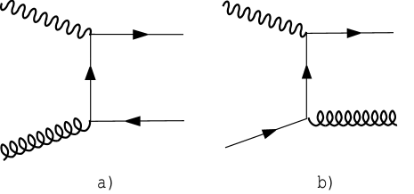
Figure 13: Leading-order Feynman diagrams for di-jet production in DIS: (a) Photon-Gluon Fusion, (b) Photon-Quark Compton scattering.

If the contribution from the quark initiated subprocess is small or the quark distribution is known, the two-jet production is a useful process to measure the gluon distribution. The di-jet invariant mass provides direct control over the fraction of the nucleon momentum carried by the gluon ($x_{G}=x_{P}$). Indeed, di-jet data from HERA have been used by the H1 and ZEUS collaborations to extract the unpolarized gluon distribution [29, 255]. With a polarized beam and target, the process is ideal for probing the polarized gluon distribution.

The unpolarized di-jet cross section for photon-nucleon collisions can be written as [118]

$$\sigma_{\rm di-jet}(q,xP)=\sigma_{\rm di-jet}^{\rm PGF}+\sigma_{\rm di-jet}^{\rm QCDC}=AG(x)+Bq(x)\ ,$$ (78)

where $G(x)$ and $q(x)$ are the gluon and quark densities, respectively, and $A$ and $B$ are the hard scattering cross sections calculable in perturbative QCD (pQCD). Similarly, the polarized cross section can be written as

$$\Delta\sigma_{\rm di-jet}(q,xP)=\sigma^{++}_{\rm di-jet}-\sigma^{+-}_{\rm dijet}=a\Delta G(x)+b\Delta q(x)\ ,$$ (79)

where the first and second $\pm$ refer to the helicities of the photon and nucleon, respectively. The double spin asymmetry for di-jet production is then

$$A_{\rm di-jet}={\Delta\sigma_{\rm di-jet}\over 2\sigma_{\rm di-jet}}={a\over A}{\Delta G(x)\over G(x)}{\sigma_{\rm di-jet}^{\rm PGF}\over 2\sigma_{\rm di-jet}}+{b\over B}{\Delta q(x)\over q(x)}{1\over 2}\left(1-{\sigma_{\rm di-jet}^{\rm PGF}\over\sigma_{\rm di-jet}}\right)\ .$$ (80)

The experimental asymmetry $A_{\rm exp}$ in DIS is related to the photon asymmetry by

$$A_{\rm exp}=P_{e}P_{N}DA_{1}^{\rm di-jet}\ ,$$ (81)

where $P_{e}$ and $P_{N}$ are the electron and nucleon polarizations, respectively, and $D$ is the depolarization factor of the photon.

At low $x$, the gluon density dominates over the quark density, and thus the photon-gluon fusion subprocess dominates. There we simply have

$$A_{1}^{\rm di-jet}={a\over A}{\Delta G(x)\over 2G(x)}\ ,$$ (82)

which provides a direct measurement of the gluon polarization. Because of the helicity selection rule, the photon and gluon must have opposite helicities to produce a quark and antiquark pair and hence $a/A=-1$. Therefore, if $\Delta G(x)$ is positive, the spin asymmetry must be negative. Leading-order calculations in Refs. [118, 141, 245, 119] show that the asymmetry is large and is strongly sensitivitive to the gluon polarization.

At NLO, the one-loop corrections for the PGF and QCDC subprocesses must be taken into account. In addition, three-jet events with two of the jets too close to be resolved must be treated as two-jet production. The sum of the virtual ($2\rightarrow 2$ processes with one loop) and real ($2\rightarrow 3$ leading-order processes) corrections are independent of the infrared divergence. However, the two-jet cross section now depends on the scheme in which the jets are defined. NLO calculations carried out in Refs. [233, 234, 246], show that the strong sensitivity of the cross section to the polarized gluon distribution survives. In terms of the spin asymmetry, the NLO effects do not significantly change the result.

Since the invariant mass of the di-jet is itself a large mass scale, two-jet production can also be used to measure $\Delta G(x)$ even when the virtuality of the photon is small or zero (real photon). A great advantage of using nearly-real photons is that the cross section is large due to the infrared enhancement, and hence the statistics are high. An important disadvantage, however, is that there is now a contribution from the resolved photons. Because the photon is nearly on-shell, it has a complicated hadronic structure of its own. The structure can be described by quark and gluon distributions which have not yet been well determined experimentally. Some models of the spin-dependent parton distributions in the photon are discussed in Ref. [155]. Leading-order calculations [270, 99] show that there are kinematic regions in which the resolved photon contribution is small and the experimental di-jet asymmetry can be used favorably to constrain the polarized gluon distribution.

5.3 $\Delta G(x)$ from Large-$p_{T}$ Hadron Production in $e-p$ Scattering

For $e-p$ scattering at moderate center-of-mass energies, such as in fixed target experiments, jets are hard to identify because of their large angular spread and the low hadron multiplicity. However one still expects that the leading hadrons in the final state reflect to a certain degree the original parton directions and flavors (discounting of course the transverse momentum, of order $\Lambda_{\rm QCD}$, from the parton intrinsic motion in hadrons and from their fragmentation). If so, one can try to use the leading high-$p_{T}$ hadrons to tag the partons produced in the hard subprocesses considered in the previous subsection.

Bravar et al. [87] have proposed to use high-$p_{T}$ hadrons to gain access to $\Delta G(x)$. To enhance the relative contribution from the photon-gluon fusion subprocess and hence the sensitivity of physical observables to the gluon distribution they propose a number of selection criteria for analysis of the data and then test these “cut” criteria in a Monte Carlo simulation of the COMPASS experiment. These simulations show that these cuts are effective in selecting the gluon-induced subprocess. Moreover, the spin asymmetry for the two-hadron production is large (10-20%) and is strongly sensitive to the gluon polarization.

Because of the large invariant mass of the hadron pairs, the underlying subprocesses can still be described in perturbative QCD even if the virtuality of the photon is small or zero [144]. This enhances the data sample but introduces additional sub-processes to the high-$p_{T}$ hadron production. The contribution from resolved photons, eg. from $\gamma\rightarrow\bar{q}q$ fluctuations, appears not to overwhelm the PGF contribution. Photons can also fluctuate into $\rho$ mesons with $\rho$-nucleon scattering yielding large-$p_{T}$ hadron pairs. Experimental information on this process can be used to subtract its contribution. After taking into account these contributions, it appears that the low-virtuality photons can be used as an effective probe of the gluon distribution to complement the data from DIS lepton scattering.

5.4 $\Delta G(x)$ from Open-charm (Heavy-quark) Production in $e-p$ Scattering

Heavy quarks can be produced in $e-p$ scattering through photon-gluon fusion and can be calculated in pQCD (see Fig. 14). In the deep-inelastic scattering region, the charm quark contribution to the $g_{1}(x,Q^{2})$ structure function is known [154],

$$g_{1}^{c}(x,Q^{2})={\alpha_{s}(\mu^{2})\over 9\pi}\int^{1}_{ax}{dy\over y}\Delta P\left({x\over y},Q^{2}\right)\Delta G(y,\mu^{2})\ ,$$ (83)

where $a=1+4m_{c}^{2}/Q^{2}$, and

$$\Delta P(x,Q^{2})=(2x-1)\ln{1+\eta\over 1-\eta}+\eta(3-4x)\ ,$$ (84)

with $\eta^{2}=1-4m_{c}^{2}x/Q^{2}(1-x)$. This result assumes that, because of the large charm quark mass, the direct charm contribution (eg. through $\Delta c(x)$) is small and the light-quark fragmentation production of charm mesons is suppressed. The $x$ dependence of the structure function, if measured, can be deconvoluted to give the polarized gluon distribution. The renormalization scale $\mu$ can be taken to be twice the charm quark mass 2$m_{c}$.

Following Ref. [111], the open charm electro-production cross section is large when $Q^{2}$ is small or vanishes and can be written

$${d^{2}\sigma^{\mu N\rightarrow c\bar{c}X}\over dQ^{2}d\nu}=\Gamma(E;Q^{2},\nu)\sigma^{\gamma^{*}N\rightarrow c\bar{c}X}(Q^{2},\nu)\ .$$ (85)

where the virtual photon flux is

$$\Gamma(E;Q^{2},\nu)={\alpha_{\rm em}\over 2\pi}{2(1-y)+y^{2}+Q^{2}/2E^{2}\over Q^{2}(Q^{2}+\nu^{2})^{1/2}}\ ,$$ (86)

$E$ and $\nu$ are the lepton and photon energies and $y=\nu/E$. For a fixed $y$, the flux is inversely proportional to $Q^{2}$. The second factor in Eq. 85 is the photonucleon cross section.

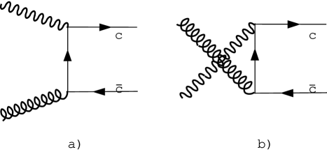
Figure 14: Feynman diagrams for charm production via Photon Gluon Fusion.

The cross section asymmetry is the simplest at the real-photon point $Q^{2}=0$. The total parton cross section for photon-gluon fusion is

$$\sigma(\hat{s})={8\pi\alpha_{\rm em}\alpha_{s}(\hat{s})\over 9\hat{s}}\left[-\beta(2-\beta^{2})+{1\over 2}(3-\beta^{4})\ln{1+\beta\over 1-\beta}\right]\ ,$$ (87)

where $\beta=\sqrt{1-4m_{c}^{2}/\hat{s}}$ is the center-of-mass velocity of the charm quark, and $\hat{s}=(q+x_{G}P)^{2}$ is the invariant mass of the photon-gluon system. On the other hand, the spin-dependent cross section is

$$\Delta\sigma={8\pi\alpha_{\rm em}\alpha_{s}(\hat{s})\over 9\hat{s}}\left[3\beta-\ln{1+\beta\over 1-\beta}\right]\ .$$ (88)

The photon-nucleon asymmetry for open charm production can be obtained by convoluting the above cross sections with the gluon distribution, giving

$$A_{\gamma N}^{c\bar{c}}(E,y)={\Delta\sigma^{\gamma N\rightarrow c\bar{c}X}\over\sigma^{\gamma N\rightarrow c\bar{c}X}}={\int_{4m_{c}^{2}}^{2MEy}d\hat{s}\Delta\hat{\sigma}(\hat{s})\Delta G(x_{G},\hat{s})\over\int_{4m_{c}^{2}}^{2MEy}d\hat{s}\hat{\sigma}(\hat{s})G(x_{G},\hat{s})}\ ,$$ (89)

where $x_{G}=\hat{s}/2M_{N}Ey$ is the gluon momentum fraction. Ignoring the $Q^{2}$ dependence, the $l-P$ spin asymmetry is related to the photon-nucleon spin asymmetry by $A_{lN}^{c\bar{c}}=DA^{c\bar{c}}_{\gamma N}$, where $D$ is the depolarization factor introduced before.

The NLO corrections have recently been calculated by Bojak and Stratmann [79] and Contogouris et al. [112]. The scale uncertainty is considerably reduced in NLO, but the dependence on the precise value of the charm quark mass is sizable at fixed target energies.

Besides the total charm cross section, one can study the distributions of the cross section in the transverse momentum or rapidity of the charm quark. The benefit of doing this is that one can avoid the region of small $x_{G}$ where the asymmetry is very small [270].

Open charm production can be measured experimentally by detecting $D^{0}$ mesons from charm quark fragmentation. On average, a charm quark has about 60% probability of fragmenting into a $D^{0}$. The $D^{0}$ meson can be reconstructed through its two-body decay mode $D^{0}\rightarrow K^{-}+\pi^{+}$; the branching ratio is about 4%. Additional background reduction can be achieved by tagging $D^{*+}\rightarrow D^{0}\pi^{+}$ through detection of the additional $\pi^{+}$.

$J/\psi$ production is, in principle, also sensitive to the gluon densities. However, because of ambiguities in the production mechanisms [184], any information on $\Delta G(x)$ is likely to be highly model-dependent.

5.5 $\Delta G(x)$ from Direct Photon Production in $p-p$ Collisions

$\Delta G(x)$ can be measured through direct (prompt) photon production in proton-proton or proton-antiproton scattering [70]. At tree level, the direct photon can be produced through two underlying subprocesses: Compton scattering $qg\rightarrow q\gamma$ and quark-antiquark annihilation $q\bar{q}\rightarrow\gamma g$, as shown in Fig. 15. In proton-proton scattering, because the antiquark distribution is small, direct photon production is dominated by the Compton process and hence can be used to extract the gluon distribution directly.

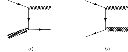
Figure 15: Feynman diagrams for Direct photon production.

Consider the collision of hadron $A$ and $B$ with momenta $P_{A}$ and $P_{B}$, respectively. The invariant mass of the initial state is $s=(P_{A}+P_{B})^{2}$. Assume parton $a$ ($b$) from the hadron $A$ ($B$) carries longitudinal momentum $x_{a}P_{A}$ ($x_{a}P_{B}$). The Mandelstam variables for the parton subprocess $a+b\rightarrow\gamma+c$ are

$$\hat{s}=x_{a}x_{b}s,~{}~{}\hat{t}=x_{a}t,~{}~{}\hat{u}=x_{b}u\ ,$$ (90)

where we have neglected the hadron mass. The parton-model cross section for inclusive direct-photon production is then

$$E_{\gamma}{d\sigma_{\rm AB}\over d^{3}p_{\gamma}}=\sum_{ab}\int dx_{a}dx_{b}f_{A}^{a}(x_{a},\mu^{2})f_{B}^{b}(x_{b},\mu^{2})E_{\gamma}{d\hat{\sigma}_{ab}\over d^{3}p_{\gamma}}\ .$$ (91)

For the polarized cross section $\Delta\sigma_{\rm AB}$, the parton distributions $f_{A,B}$ are replaced by polarized distributions $\Delta f_{A,B}$, and the parton cross sections $\hat{\sigma}_{ab}$ are replaced by the spin-dependent cross section $\Delta\hat{\sigma}_{ab}$. The tree-level parton scattering cross section is

$$E_{\gamma}{d\hat{\sigma}\over d^{3}p_{\gamma}}=\alpha_{\rm em}\alpha_{s}{1\over\hat{s}}|M|^{2}\delta(\hat{s}+\hat{t}+\hat{u})\ ,$$ (92)

where the $\delta$-function reduces the parton momentum integration into one integration over, say, $x_{a}$ with range $[-u/(s+t),1]$ and

$$|M|^{2}_{qg\rightarrow\gamma q}=-{1\over 2}{\hat{s}^{2}+\hat{t}^{2}\over\hat{s}\hat{t}};~{}~{}~{}|M|^{2}_{q\bar{q}\rightarrow\gamma g}={8\over 9}{\hat{u}^{2}+\hat{t}^{2}\over\hat{u}\hat{t}}\ .$$ (93)

For the polarized case, we have the same expression as in Eq. (92) but with

$$|\Delta M|^{2}_{qg\rightarrow\gamma q}=-{1\over 2}{\hat{s}^{2}-\hat{t}^{2}\over\hat{s}\hat{t}};~{}~{}~{}|\Delta M|^{2}_{q\bar{q}\rightarrow\gamma g}=-{8\over 9}{\hat{u}^{2}+\hat{t}^{2}\over\hat{u}\hat{t}}\ .$$ (94)

In the energy region where the Compton subprocess is dominant, we can write the proton-proton cross section in terms of the deep-inelastic structure functions $F_{2}$ and $g_{1}$ and the gluon distributions $G$ and $\Delta G$ [70],

$$E_{\gamma}{d\sigma_{\rm AB}\over d^{3}p_{\gamma}} = \int dx_{a}dx_{b}\left[{F_{2}(x_{a},\mu^{2})\over x_{a}}G(x_{b},\mu^{2})E_{\gamma}{d\hat{\sigma}_{qg}\over d^{3}p_{\gamma}}+(x_{a}\rightarrow x_{b})\right]\ ,$$

$$E_{\gamma}{d\Delta\sigma_{\rm AB}\over d^{3}p_{\gamma}} = \int dx_{a}dx_{b}\left[{2g_{1}(x_{a},\mu^{2})\over x_{a}}\Delta G(x_{b},\mu^{2})E_{\gamma}{d\Delta\hat{\sigma}_{qg}\over d^{3}p_{\gamma}}+(x_{a}\rightarrow x_{b})\right]\ .$$ (95)

Here the factorization scale $\mu$ is usually taken as the photon transverse momentum $p_{T}$.

Unfortunately, the above simple picture of direct photon production is complicated by high-order QCD corrections. Starting at next-to-leading order the inclusive direct-photon production cross section is no longer well defined because of the infrared divergence arising when the photon momentum is collinear with one of the final state partons. To absorb this divergence, an additional term must be added to Eq. (91) which represents the production of jets and their subsequent fragmentation into photons. Therefore, the total photon production cross section depends also on these unknown parton-to-photon fragmentation functions. Moreover, the separation into direct photon and jet-fragmented photon is scheme-dependent as the parton cross section $E_{\gamma}d\hat{\sigma}_{ab}/d^{3}p_{\gamma}$ depends on the methods of infrared subtraction [147].

To minimize the influence of the fragmentation contribution, one can impose an isolation cut on the experimental data [139]. Of course the parton cross section entering Eq. (91) must be calculated in accordance with the cut criteria. An isolation cut has the additional benefit of excluding photons from $\pi^{0}$ or $\eta$ decay. When a high-energy $\pi^{0}$ decays, occasionally the two photons cannot be resolved in a detector or one of the photons may escape detection. These backgrounds usually reside in the cone of a jet and are largely excluded when an isolation cut is imposed.

The NLO parton cross sections in direct photon production have been calculated for both polarized and unpolarized scattering [147]. Comparison between the experimental data and theory for the latter case is still controversial. While the collider data at large $p_{T}$ are described very well by the NLO QCD calculation [1], the fixed-target data and collider data at low-$p_{T}$ are under-predicted by theory. Phenomenologically, this problem can be solved by introducing a broadening of the parton transverse momentum in the initial state [51]. Theoretical ideas attempting to resolve the discrepancy involve a resummation of threshold corrections [215] as well as a resummation of double logarithms involving the parton transverse momentum [212, 102]. Recently, it has been shown that a combination of both effects can reduce the discrepancy considerably [213].

5.6 $\Delta G(x)$ from Jet and Hadron Production in $p-p$ Collisions

Jets are produced copiously in high-energy hadron colliders. The study of jets is now at a mature stage as the comparison between experimental data from Tevatron and other facilities and the NLO QCD calculations are in excellent agreement. Therefore, single and/or di-jet production in polarized colliders can be an excellent tool to measure the polarized parton distributions, particularly the gluon helicity distribution [84].

There are many underlying subprocesses contributing to leading-order jet production: $qq^{\prime}\rightarrow qq^{\prime}$, $q\bar{q}^{\prime}\rightarrow q\bar{q}^{\prime}$, $qq\rightarrow qq$, $q\bar{q}\rightarrow q^{\prime}\bar{q}^{\prime}$, $q\bar{q}\rightarrow q\bar{q}$, $q\bar{q}\rightarrow gg$, $gg\rightarrow q\bar{q}$, $qg\rightarrow qg$, $gg\rightarrow gg$. Summing over all pairs of initial partons $ab$ and subprocess channels $ab\rightarrow cd$, and folding in the parton distributions $f_{a/A}(x_{a})$, etc., in the initial hadrons $A$ and $B$, the net two-jet cross section is

$${d\sigma\over d^{3}p_{c}}=\sum_{abcd}\int dx_{a}dx_{b}f_{a/A}(x_{a})f_{b/B}(x_{b}){d\hat{\sigma}\over d^{3}p_{c}}(ab\rightarrow cd)\ .$$ (96)

For jets with large transverse momentum, it is clear that the valence quarks dominate the production. However, for intermediate and small transverse momentum, jet production is overwhelmed by gluon-initiated subprocesses.

Studies of the NLO corrections are important in jet production because the QCD structure of the jets starts at this order. For polarized scattering, this has been investigated in a Monte Carlo simulation recently [113]. The main result of the study shows that the scale dependence is greatly reduced. Even though the jet asymmetry is small, because of the large abundance of jets, the statistical error is actually very small.

Besides jets, one can also look for leading hadron production, just as in electroproduction considered previously. This is useful particularly when jet construction is difficult due to the limited geometrical coverage of the detectors. One generally expects that the hadron-production asymmetry has the same level of sensitivity to the gluon density as the jet asymmetry.

5.7 Experimental Measurements

The first information on $\Delta G$ has come from NLO fits to inclusive deep-inelastic scattering data as discussed in Sec. 3.5. Also recent semi-inclusive data from the HERMES experiment indicates a positive gluon polarization at a moderate $x_{G}$. Future measurements from COMPASS at CERN, polarized RHIC, and polarized HERA promise to provide much more accurate data.

5.7.1 Inclusive DIS Scattering

As discussed in Sec. 3.5, the spin-dependent structure function $g_{1}(x,Q^{2})$ is sensitive to the gluon distribution at NLO. However, to extract the gluon distribution, which appears as an additive term, one relies on the different $Q^{2}$-dependence of the quark and gluon contributions.

The biggest uncertainty in the procedure of the NLO fits is the parametric form of the gluon distribution at $Q_{0}^{2}$. It is known that by taking different parameterizations, one can get quite different results.

5.7.2 HERMES Semi-inclusive Scattering

The HERMES experiment has been described in Sec. 2.3. In a recent publication [32], the HERMES collaboration reported a first measurement of the longitudinal spin asymmetry $A_{||}=-0.28\pm 0.12\pm 0.02$ in the photoproduction of pairs of hadrons with high transverse momentum $p_{T}$, which translate into a $\langle\Delta G/G\rangle=0.41\pm 0.18\pm 0.03$ at an average $\langle x_{G}\rangle=0.17$.

Following the proposal of Ref. [87], the data sample contains hadron pairs with opposite electric charge. The momentum of the hadron is required to be above 4.5 GeV/c with a transverse component above 0.5 GeV/c. The minimum value of the invariant mass of the two hadrons, in the case of two pions, is 1.0 GeV/c². A nonzero asymmetry is observed if the pairs with $p_{T}^{h_{1}}>1.5$ GeV/c and $p_{T}^{h_{2}}>1.0$ GeV/c are selected. The measured asymmetry is shown in Fig. 16 with an average $Q^{2}$ of 0.06(GeV/c)². If $p_{T}^{h_{1}}>1.5$ GeV/c is not enforced the asymmetry is consistent with zero.

Figure 16: Data for high $p_{T}$ hadrons from the HERMES experiment [32] showing (left) the asymmetry and (right) the extracted gluon polarization.

The measured asymmetry was interpreted in terms of the following processes: lowest-order deep-inelastic scattering, vector-dominance of the photon, resolved photon, and hard QCD processes – Photon Gluon Fusion and QCD Compton effects. The PYTHIA [263] Monte Carlo generator was used to provide a model for the data. In the region of phase space where a negative asymmetry is observed, the simulated cross section is dominated by photon gluon fusion. The sensitivity of the measured asymmetry to the polarized gluon distribution is also shown Fig. 16. Note that the analysis does not include NLO contributions which could be important. The HERMES collaboration will have more data on this process in the near future.

5.7.3 COMPASS Experiment

The COMPASS expriment at CERN will use a high-energy (up to 200 GeV) muon beam to perform deep-inelastic scattering on nucleon targets, detecting final state hadron production [111]. The main goal of the experiment is to measure the cross section asymmetry for open charm production to extract the gluon polarization $\Delta G$.

For the charm production process, COMPASS estimates a charm production cross section of 200 to 350 nb. With a luminosity of $4.3\times 10^{37}$ cm^-2day^-1, they predict about 82,000 charm events in this kinematic region per day. Taking into account branching ratios, the geometrical acceptance and target rescattering, etc., 900 of these events can be reconstructed per day. The number of background events is on the order of 3000 per day. Therefore the total statistical error on the spin asymmetry will be about $\delta A_{\gamma N}^{c\bar{c}}=0.076$.

Figure 17: Predictions of the open charm asymmetry for the COMPASS experiment. The curves are predictions for three representative gluon spin distributions [151]. Also shown are typical error bars expected from the measurement.

Shown in Fig. 17 are the predicted asymmetries $A_{\gamma N}^{c\bar{c}}$ and $A_{\mu N}^{c\bar{c}}$ for open charm production as a function of $y$. The curves correspond to three different models for $\Delta G$. From the results at different $y$, one hopes to get some information about the variation of $\Delta G$ as a function of $x$. Measurements with high $p_{T}$ hadrons will also be used to complement the information from charm production.

5.7.4 $\Delta G(x)$ from RHIC Spin Experiments

One of the primary goals of the RHIC spin experiments is to determine the polarized gluon distribution. This can be done with direct photon, jet, and heavy quark production.

Figure 18: Projected sensitivity [147] to the gluon polarization from direct photon production at RHIC with the PHENIX detector. The curves represent different assumptions for the gluon spin distribution [151, 156].

Direct photon production is unique at RHIC. This can either be done on inclusive direct photon events (PHENIX) or photon-plus-jet events (STAR). Estimates of the background from $q\bar{q}$ annihilation show a small effect. Shown in Fig. 18 is the sensitivity of STAR measurements of $\Delta G(x)$ in the channel $\vec{p}\vec{p}\rightarrow\gamma+{\rm jet}+X$. The solid line is the input distribution and the data points represent the reconstructed $\Delta G(x)$. For inclusive direct photon events, simulations show very different spin asymmetries from different spin-dependent gluon densities.

Jet and heavy flavor productions are also favorable channels to measure polarized gluons at RHIC. The interested reader can consult the recent review in Ref. [91].

5.7.5 $\Delta G(x)$ from Polarized HERA

The idea of a polarized HERA collider ($\vec{e}^{-}-\vec{p}$) has been described in Sec 2.4. Here we highlight a few experiments which can provide a good measurement of the polarized gluon distribution [120].

First of all, polarized HERA will provide access to very large $Q^{2}$ and low $x$ regions compared with fixed-target experiments. At large $x$, $Q^{2}$ can be as large as $10^{4}$ GeV². Thus, one can probe the gluon distribution through the $Q^{2}$ variation of the $g_{1}$ structure function. An estimate from an NLO pQCD analysis shows that the polarized HERA data on $g_{1}$ can reduce the uncertainty on the total gluon helicity to $\pm 0.2$(exp)$\pm 0.3$(theory).

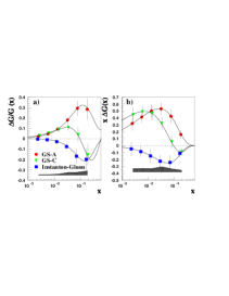
Figure 19: Projected statistical and systematic error bars for the polarized gluon distribution using two-jet production with polarized $e-p$ collisions at HERA. The curves represent different assumptions about the gluon spin distribution [151].

Polarized HERA can also measure the polarized gluon distribution through di-jet production. Assuming a luminosity 500 $pb^{-1}$ and with the event selection criteria $5<Q^{2}<100$ GeV², $0.3<y<0.85$ and $p_{T}^{\rm jet}>5$ GeV, the expected error bars on the extracted $\Delta G(x)$ are shown in Fig. 19. The measured $x$ region covers $0.002<x_{G}<0.2$. $\Delta G(x)$ can also be measured at polarized HERA through high-$p_{T}$ hadrons and jet production with real photons.

6 Transverse Spin Physics

6.1 The $g_{2}(x,Q^{2})$ Structure Function of the Nucleon

As discussed in Sec. 3.2, the structure function $g_{2}(x,Q^{2})$ can be measured with a longitudinally polarized lepton beam incident on a transversely polarized nucleon target. For many years, theorists have searched for a physical interpretation of $g_{2}(x,Q^{2})$ in terms of a generalization of Feynman’s parton model [142, 210], as most of the known high-energy processes can be understood in terms of incoherent scattering of massless, on-shell and collinear partons [142]. It turns out, however, that $g_{2}$ is an example of a higher-twist structure function.

Higher-twist processes cannot be understood in terms of the simple parton model [138]. Instead, one has to consider parton correlations initially present in the participating hadrons. Higher-twist processes can be described in terms of coherent parton scattering in the sense that more than one parton from a particular hadron takes part in the scattering. Higher-twist observables are interesting because they represent the quark and gluon correlations in the nucleon which cannot otherwise be studied.

Why does $g_{2}(x,Q^{2})$ contain information about quark and gluon correlations? According to the optical theorem, $g_{2}(x,Q^{2})$ is the imaginary part of the spin-dependent Compton amplitude for the process

$$\gamma^{*}(+1)+N(1/2)\rightarrow\gamma^{*}(0)+N(-1/2)$$ (97)

where $\gamma^{*}$ and $N$ represent the virtual photon and nucleon, respectively, and the labels in the brackets are helicities. Thus Compton scattering involves a $t$-channel helicity exchange. When the process is factorized in terms of parton subprocesses, the intermediate partons must carry this helicity exchange. Because of the vector coupling, massless quarks cannot undergo helicity flip in perturbative processes. Nonetheless, the required helicity exchange is fulfilled in two ways in QCD: first, through single quark scattering in which the quark carries one unit of orbital angular momentum through its transverse momentum; second, through quark scattering with an additional transversely-polarized gluon from the nucleon target. These two mechanisms are combined in such a way to yield a gauge-invariant result.

To leading order in $\alpha_{s}$, $g_{2}(x_{B},Q^{2})$ can be expressed in terms of a simple parton distribution $\Delta q_{T}(x)$ [172],

$$g_{2}(x_{B},Q^{2})={1\over 2}\sum_{i}e_{i}^{2}(\Delta q_{iT}(x_{B},Q^{2})+\Delta\bar{q}_{iT}(x_{B},Q^{2}))\ ,$$ (98)

where

$$\Delta q_{T}(x)={1\over 2M}\int{d\lambda\over 2\pi}e^{i\lambda x}\langle PS_{\perp}|\bar{q}(0)\gamma_{\perp}\gamma_{5}q(\lambda n)|PS_{\perp}\rangle\ ,$$ (99)

and $S_{\perp}$ is the transverse polarization vector and $\gamma_{\perp}$ is the component along the same direction. Although it allows a simple estimate of $g_{2}$ in the models [180], the above expression is deceptive in its physical content. It has led to incorrect identifications of twist-three operators [26, 258] and incorrect next-to-leading order coefficient functions [204]. When the leading-logarithmic corrections were studied, it was found that $\Delta q_{T}(x,Q^{2})$ mixes with other distributions under scale evolution [261]. In fact, $\Delta q_{T}(x,Q^{2})$ is a special moment of more general parton distributions involving two light-cone variables

$$\Delta q_{T}(x)={2\over x}\int^{1}_{-1}dy\left(K_{1}(x,y)+K_{2}(x,y)\right)\ ,$$ (100)

where the $K_{i}(x,y)$ are defined as

$$\int{d\lambda\over 2\pi}{d\mu\over 2\pi}e^{ix\lambda+i\mu(y-x)}\langle PS|\bar{\psi}(0)iD^{\alpha}(\mu n)\psi(\lambda n)|PS\rangle$$ (101)

$$= S^{\alpha}\gamma_{5}\not\!pK_{1}(x,y)+iT^{\alpha}\not\!pK_{2}(x,y)+...$$

where $T^{\alpha}=\epsilon^{\alpha\beta\gamma\delta}S_{\perp}p_{\gamma}n_{\delta}$. Under a scale transformation, the general distributions $K_{i}(x,y)$ evolve autonomously while the $\Delta q_{iT}(x)$ do not [90, 131]. The first result for the leading logarithmic evolution of the twist-three distributions (and operators) [90] has now been confirmed by many studies [252, 60].

Thus an all-order $g_{2}$ factorization formula is much more subtle than is indicated by the leading-order result. It involves the generalized two-variable distributions, $K_{i}(x,y)$,

$$g_{T}(x_{B},Q^{2})=\sum_{ia}\int^{1}_{-1}{dxdy\over xy}\left(C_{a}\left({x_{B}\over x},{x_{B}\over y},\alpha_{s}\right)K_{i}(x,y)+(x_{B}\rightarrow-x_{B})\right)\ ,$$ (102)

where $C_{a}$ are the coefficient functions with $a$ summing over different quark flavors and over gluons. Accordingly, a perturbative calculation of $g_{2}$ in terms of quark and gluon external states must be interpreted carefully [228]. Recently, the complete one-loop radiative corrections to the singlet and non-singlet $g_{2}$ have been published [192]. The result is represented as the order-$\alpha_{s}$ term in $C_{i}$ and is one of the necessary ingredients for a NLO analysis of $g_{2}$ data. Note that the Burkhardt-Cottingham sum rule, $\int^{1}_{0}g_{2}(x,Q^{2})dx=0$, survives the radiative corrections provided the order of integrations can be exchanged [96].

As an example of the interesting physics associated with $g_{2}$, we consider its second moment in $x$

$$\int^{1}_{0}dxxg_{2}(x,Q^{2})={1\over 3}\left(-a_{2}(Q^{2})+d_{2}(Q^{2})\right)\ ,$$ (103)

where $a_{2}(Q^{2})$ is the second moment of the $g_{1}(x)$ structure function. Here $d_{2}(Q^{2})$ is the matrix element of a twist-three operator,

$$\langle PS|{1\over 4}\bar{\psi}g\tilde{F}^{\sigma(\mu}\gamma^{\nu)}\psi|PS\rangle=2d_{2}S^{[\sigma}P^{(\mu]}P^{\nu)}\ ,$$ (104)

where $\tilde{F}^{\mu\nu}=(1/2)\epsilon^{\mu\nu\alpha\beta}F_{\alpha\beta}$, and the different brackets – $(\cdots)$ and $[\cdots]$ – denote symmetrization and antisymmetrization of indices, respectively. The structure of this twist-three operator suggests that it measures a quark and a gluon amplitude in the initial nucleon wave function.

To better understand the significance of $d_{2}(Q^{2})$, we consider a polarized nucleon in its rest frame and consider how the gluon field inside of the nucleon responds to the polarization. Intuitively, because of parity conservation, the color magnetic field $\vec{B}$ can be induced along the nucleon polarization and the color electric field $\vec{E}$ in the plane perpendicular to the polarization. Introducing the color-singlet operators $\hat{O}_{B}=\psi^{\dagger}g\vec{B}\psi$ and $\hat{O}_{E}=\psi^{\dagger}\vec{\alpha}\times g\vec{E}\psi$, we define the gluon-field polarizabilities $\chi_{B}$ and $\chi_{E}$ in the rest frame of the nucleon,

$$\langle PS|\hat{O}_{B,E}|PS\rangle=\chi_{B,E}2M^{2}\vec{S}\ .$$ (105)

Then it is easy to show

$$d_{2}=(2\chi_{B}+\chi_{E})/3\ .$$ (106)

Thus $d_{2}$ measures the response of the color electric and magnetic fields to the polarization of the nucleon.

The experimental measurements of the $g_{2}$ structure function started with the SMC [14] and E142 [45, 46] collaborations. Subsequently, the E143 [5], E154 [7], and E155 [47, 83] collaborations have also measured and published their data. The combined E143 and E155 data for proton and deuteron are shown in Fig. 20. The solid line shows the twist-two contribution to $g_{2}$ only [278]. The dashed and dash-dotted lines are the bag model calculations by Song [267] and Stratmann [269].

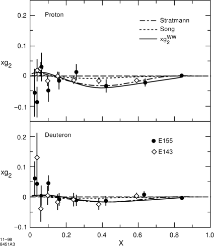
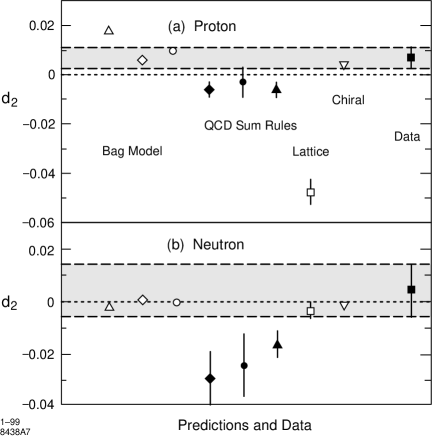
Figure 20: (Upper) Data for $g_{2}$ for the proton and deuteron from E143 [5] and E155 [47] collaborations. (Lower) Comparison between data and calculations for $d_{2}$, the second moment of $g_{2}$.

Neglecting the contributions from $x<0.02$ and $x>0.8$ and the $Q^{2}$ dependence, the E155 collaboration [47, 83] has integrated their data to get $\int dxg_{2}^{p}=-0.022\pm 0.071$ and $\int dxg_{2}^{d}=0.023\pm 0.044$. The results are consistent with the Burkardt-Cottingham sum rules within the relatively large errors. The second moments allow an extraction of the $d_{2}$ matrix elements. E155 found $d_{2}^{p}=0.005\pm 0.008$ and $d_{2}^{d}=0.008\pm 0.005$ at an average $Q^{2}$ of 5 GeV². A combined analysis of the E142, E143, E154, and E155 data yields $d_{2}^{p}=0.007\pm 0.004$ and $d_{2}^{n}=0.004\pm 0.010$. These numbers are generally consistent with bag model [267, 269, 198, 193] and chiral quark model [279] estimates, and are 1 to $2\sigma$ away from QCD sum rule calculations [268, 62, 134]. The error bars on the present lattice calculation are still relatively large [159].

According to the simple quark model, the $d_{2}$ matrix element in the neutron should be much smaller than that in the proton because of SU(6) spin-flavor symmetry. While the proton $d_{2}$ has been constrained with reasonable precision, the neutron $d_{2}$ has a much larger error bar. In the near future, JLab experiments with a polarized ${}^{3}He$ target [59] can improve the present error on the neutron $d_{2}$ and hence test the quark model predictions.

6.2 Tranversity Distribution

Along with the unpolarized and polarized quark distributions - $q_{i}(x,Q^{2})$ and $\Delta q_{i}(x,Q^{2})$ - discussed above, a third quark distribution exists at the same order (twist two) as the other two distributions. Note that no corresponding transverse spin distribution exists for gluons (due to helicity conservation).

This transversity distribution, $\delta q_{i}(x,Q^{2})$, can be described in the Quark-Parton Model as the difference in the distribution of quarks with spin aligned along the nucleon spin vs. anti-aligned for a nucleon polarized transverse to its momentum. The structure function related to transversity is given by

$$h_{1}(x,Q^{2})={1\over 2}\sum_{i}e_{i}^{2}\delta q_{i}(x,Q^{2})\ .$$ (107)

The first moment of the transversity distributions also leads to an interesting observable - the nucleon’s tensor charge $a^{t}_{i}$:

$$a^{t}_{i}=\int_{0}^{1}\left[\delta q_{i}(x)-\delta\bar{q}_{i}(x)\right]dx\ .$$ (108)

In terms of nucleon matrix elements, this tensor charge is defined [168] as:

$$2a^{t}_{i}\left(S^{\mu}P^{\nu}-S^{\nu}P^{\mu}\right)=\langle PS|\bar{\psi}_{i}\sigma^{\mu\nu}i\gamma_{5}\psi_{i}|PS\rangle\ .$$ (109)

Recent calculations have made estimates of the tensor charges using QCD Sum Rules [169, 199], Lattice QCD [50], and within the Chiral Quark Model [202].

In a non-relativistic model the transversity is equal to the longitudinal spin distribution ($\delta q_{i}=\Delta q_{i}$) because the distribution would be invariant under the combination of a rotation and a Lorentz boost. Relativistically, this is not the case and $\delta q_{i}$ could be significantly different from $\Delta q_{i}$. The challenge to gaining experimental information on $\delta q_{i}$ lies in its chiral structure. In the helicity basis [181, 182] $\delta q_{i}$ represents a quark helicity flip, which cannot occur in any hard process for massless quarks within QED or QCD. This chiral-odd property of transversity makes it unobservable in inclusive DIS. In order to observe $h_{1}(x,Q^{2})$ a second non-perturbative process that is also chiral-odd must take place. This was first discussed by Ralston and Soffer [251] in connection with Drell-Yan production of di-muons in polarized $p-p$ collisions. Here the transversity distribution of both protons results in a chiral-even interaction.

Several calculations have suggested that the transversity distribution may be accessible in semi-inclusive lepton-nucleon scattering [108, 183, 206, 236, 41]. In this process a chiral-odd fragmentation function, leading to a lepto-produced hadron, offsets the chiral-odd transversity distribution. Many of these calculations take advantage of an inequality

$$|\delta q_{i}(x)|\leq{q_{i}(x)+\Delta q_{i}(x)\over 2}$$ (110)

discovered by Soffer [264] to limit the possible magnitude of $h_{1}(x)$.

Calculations [206, 236, 207] have also detailed a set of spin distribution and fragmentation functions that are accessible from leading and next-to-leading twist processes. In fact in some cases the next-to-leading twist processes can dominate, especially at low $Q^{2}$ and with longitudinally polarized targets.

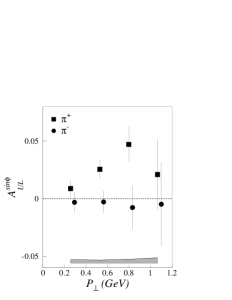
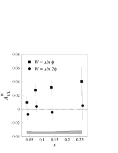
Figure 21: Single spin asymmetry for pion electroproduction from the HERMES experiment [33] vs. $p_{T}$ (left) and $x$ (right).

Potentially relevant experimental information has recently come from the HERMES collaboration and SMC collaboration. HERMES has measured the single-spin azimuthal asymmetry for pions produced in deep-inelastic scattering of unpolarized positrons from a longitudinally polarized hydrogen target [33] (see Fig. 21). A related measurement has been reported by SMC [88] using a transversely polarized target. The HERMES asymmetry is consistent with a $\sin\phi$ distribution, where $\phi$ is the angle between the lepton scattering plane and the plane formed by the virtual photon and pion momenta. While the $x$ dependence of the asymmetry is relatively weak except for the smallest $x=0.04$ point, the $p_{T}$ dependence shows a rapid rise up to 0.8 GeV^-1. The average $\pi^{+}$ asymmetry averaged over the full acceptance is $0.022\pm 0.005\pm 0.003$ while the asymmetry for $\pi^{-}$ production is consistent with zero. Some models [133] suggest that the product of the transversity distribution times the chiral-odd fragmentation function can account for the observed asymmetry.

Transversity may also play a role in observed single-spin asymmetries in $p-p$ collisions. These possibilities are discussed in the next section.

6.3 Single-Spin Asymmetries From Strong Interactions

As we have discussed in Sec. 4.2, single-spin asymmetries can arise from processes involving parity-violating interactions, such as $W$ and $Z$ boson production in $\vec{p}-p$ collisions at RHIC. In this subsection, we discuss a different class of single-spin asymmetries which are generated entirely from strong interaction effects. While we do not have enough space here to make a thorough examination of the subject, we briefly discuss the phenomena, a few leading theoretical ideas, and some other related topics. A recent review of the subject can be found in Ref. [222].

For more than two decades, it has been known that in hadron-hadron scattering with one beam transversely polarized, the single-particle inclusive yield at nonzero $p_{T}$ has an azimuthal dependence in a coordinate system where $z$ is chosen to lie along the direction of the polarized beam, and $x$ along the beam polarization [203]. It is easy to see that the angular dependence is allowed by strong interaction dynamics. If the momentum of the polarized beam is $\vec{p_{b}}$ and that of the observed particle $\vec{p_{o}}$, the angular distribution reflects the existence of a triple correlation,

$$\vec{p}_{b}\times\vec{p}_{o}\cdot\vec{S}\ ,$$ (111)

where $\vec{S}$ is the beam polarization. The correlation conserves parity and hence is not forbidden in strong interactions. Although it is nominally time-reversal odd, the minus sign can be canceled, under the time-reversal transformation, by a factor of $i$ from an interference of two amplitudes with different phase factors.

The angular correlation is usually characterized by the spin asymmetry

$$A_{N}(x_{F},p_{T})={d\sigma^{\uparrow}-d\sigma^{\downarrow}\over d\sigma^{\uparrow}+d\sigma^{\downarrow}}\ ,$$ (112)

where $d\sigma^{\uparrow,\downarrow}$ are the cross sections with reversed polarizations, and $p_{T}$ is the transverse momentum of the produced particle. $x_{F}$ is the Feynman $x$ variable, $x_{F}=p_{L}/p_{L}^{\rm max}$, where $p_{L}$ is the longitudinal momentum of the produced hadron and $p_{L}^{\rm max}$ is the maximum allowed longitudinal momentum. An example of a single spin asymmetry for $\pi$ production is shown in Fig. 22. After examining the existing data, one finds the following interesting systematic effects [222]:

• $A_{N}$ is significant only in the fragmentation region of the polarized beam. It increases almost linearly with $x_{F}$ when the target is unpolarized.

• $A_{N}$ is large only for moderate transverse momentum $p_{T}$.

• $A_{N}$ and its sign show a strong dependence on the type of polarized beam ($p,\bar{p}$) and produced particles ($\pi^{\pm},\pi_{0}$).

That $A_{N}$ is strikingly large is the most impressive aspect of the phenomenon.

Figure 22: Measured single-spin asymmetries from $\pi^{\pm}$ production in $\vec{p}-p$ scattering (left) and $\pi^{0}$ production in $\vec{p}-p$ and $\vec{p}-\bar{p}$ scattering (right) at Fermilab [203]. The curves are theoretical fits from Ref. [244].

The simplest theory explaining $A_{N}$ is one that assumes an underlying parton process: partons from the parent hadrons scatter and fragment to produce the observed particle. To get the single spin asymmetry, one requires, for instance, that quarks change their helicity during hard scattering. However, chiral symmetry then dictates that the asymmetry is proportional to the quark mass $m_{q}$ which is vanishingly small for light quarks. Thus the simple parton model for $A_{N}$ cannot yield the magnitude of the observed symmetry [200].

For the moment, the leading theoretical ideas in the literature are still based on the parton degrees of freedom. However, the spin-flip is introduced through more complicated mechanisms: Either the initial and final partons are assumed to have novel nonpertrubative distribution and fragmentation functions, respectively, or the parton hard scattering involves coherent processes.

In the latter case, the asymmetry can arise from the coupling of chiral even (odd) twist-two (twist-three) parton correlations in the polarized nucleon and chiral even (odd) twist-three (twist-two) fragmentation functions of the scattered partons [132, 243, 185, 244]. The required phase difference is generated from the interference of the hard scattering amplitudes in which one of the hard propagators is on-shell. The predicted asymmetry is of order $\Lambda_{\rm QCD}/p_{T}$ in the large $p_{T}$ limit, which is a characteristic twist-three effect. For moderate $p_{T}$, $A_{N}$ can be a slowly decreasing function of $p_{T}$ [244]. The comparison between the experimental data and the phenomenological prediction seems to yield good agreement [244]. It is not clear, however, that the available fixed target data can be fully described by perturbative parton scattering. One needs more data at higher energy to test the scaling property inherent in a perturbative description.

The alternative is to consider nonperturbative mechanisms to generate the phase difference. This can be done by introducing transverse-momentum dependent parton distributions [262] and fragmentation functions [108]. In a transversely polarized nucleon, the transverse momentum distribution may not be rotationally invariant. It may depend on the relative orientation of the spin and momentum vectors. Likewise, when a transversely polarized quark fragments, the amplitude for hadron production can depend on the relative orientation between the hadron momentum and the quark spin. Both mechanisms have been shown to produce large single spin asymmetries [41, 76, 78, 42]. Here again the applicability of the model for the existing data is not clear. In particular, the fitted fragmentation functions and parton distributions must be tested in different kinematic regions. Moreover, the new distributions do not possess color gauge invariance.

A phenomenological model for parton scattering with formation of large-$p_{T}$ hadrons was proposed by Boros, Liang and Meng [81]. Although not derived from field theory, the model has a very intuitive physical picture and successfully describes the data. It would be interesting to test the predictive power of the model in future experiments. The RHIC spin facility can test many of these theoretical ideas with a variety of experimental probes including [254] polarized Drell-Yan, dimeson production, etc.

A subject closely related to the single-spin asymmetry is the polarization of hyperons, such as $\Lambda$, produced in unpolarized hadron collisions [171]. The observed polarization is perpendicular to the plane formed by the beam and hyperon momenta. Many theoretical models have been invented to explain the polarization [140]. Most models are closely related to those devised to explain the single spin asymmetry.

7 Off-Forward Parton Distributions

In this section, we discuss some of the recent theoretical developments on generalized (off-forward) parton distributions (OFPD) and their relation to the angular momentum distributions in the nucleon. We will also consider possible experimental processes, such as deeply virtual Compton scattering (DVCS) and meson production, to measure these novel distributions.

OFPD’s were first introduced in Ref. [123] and discovered independently in Ref. [186] in studying the spin structure of the nucleon. Radyushkin and others have introduced slightly different versions of the distributions, but the physical content is the same [247, 248, 249, 110]. The other names for these functions range from off-diagonal, non-forward and skewed to generalized parton distributions. Here we follow the discussion in Ref. [189].

One of the most important sources of information about the nucleon structure is the form factors of the electroweak currents. It is well known that the vector current yields two form factors

$$\langle P^{\prime}|\overline{\psi}\gamma^{\mu}\psi|P\rangle=F_{1}(Q^{2})\overline{U}\gamma^{\mu}U+F_{2}(Q^{2})\overline{U}{i\sigma^{\mu\nu}q_{\nu}\over 2M}U\,,$$ (113)

where $q_{\nu}=P^{\prime}-P$ and $F_{1}$ and $F_{2}$ are the Dirac and Pauli form factors, respectively. $F_{2}$ gives the anomalous magnetic moment of the nucleon, $\kappa=F_{2}(0)$. The charge radius of the nucleon is defined by

$$\langle r^{2}\rangle=-6\left.{dG_{E}(Q^{2})\over dQ^{2}}\right|_{Q^{2}=0}\,,$$ (114)

with $G_{E}=F_{1}-Q^{2}/(4M^{2})F_{2}$. The axial vector current also defines two form factors,

$$\langle P^{\prime}|\overline{\psi}\gamma^{\mu}\gamma_{5}\psi|P\rangle=G_{A}(Q^{2})\overline{U}\gamma^{\mu}\gamma_{5}U+G_{P}(Q^{2})\overline{U}{\gamma_{5}q^{\mu}\over 2M}U(P)\,.$$ (115)

The axial form factor $G_{A}$ is related to the fraction of the nucleon spin carried by the spin of the quarks, $\Delta\Sigma$, and can be measured from polarized deep inelastic scattering as discussed in previous sections. The pseudoscalar charge, $G_{P}(0)$, can be measured in muon capture.

A generalization of the electroweak currents can be made through the following sets of twist-two operators,

$$O_{q}^{\mu_{1}\cdots\mu_{n}} = \overline{\psi}_{q}\gamma^{(\mu_{1}}iD^{\mu_{2}}\cdots iD^{\mu_{n})}\psi\,$$

$$\tilde{O}_{q}^{\mu_{1}\cdots\mu_{n}} = \overline{\psi}_{q}\gamma^{(\mu_{1}}\gamma_{5}iD^{\mu_{2}}\cdots iD^{\mu_{n})}\psi\,,$$ (116)

where all indices $\mu_{1}\cdots\mu_{n}$ are symmetric and traceless as indicated by (…) in the superscripts. These operators form the totally symmetric representation of the Lorentz group. One can also introduce gluon currents through the operators:

$$O_{g}^{\mu_{1}\cdots\mu_{n}} = F^{(\mu_{1}\alpha}iD^{\mu}_{2}\cdots iD^{\mu_{n-1}}F_{\alpha}^{~{}\mu_{n})}$$

$$\tilde{O}_{g}^{\mu_{1}\cdots\mu_{n}} = F^{(\mu_{1}\alpha}iD^{\mu}_{2}\cdots iD^{\mu_{n-1}}\tilde{F}_{\alpha}^{~{}\mu_{n})}\,.$$ (117)

For $n>1$, the above operators are not conserved currents from any global symmetry. Consequently, their matrix elements depend on the momentum-transfer scale $\mu$ at which they are probed. For the same reason, there is no low-energy probe that couples to these currents.

One can then define the generalized charges $a_{n}(\mu^{2})$ from the forward matrix elements of these currents

$$\langle P|O^{\mu_{1}\cdots\mu_{2}}|P\rangle=2a_{n}(\mu^{2})P^{(\mu_{1}}P^{\mu_{2}}\cdots P^{\mu_{n})}\,.$$ (118)

The moments of the Feynman parton distribution $q(x,\mu^{2})$ are related to these charges

$$\int^{1}_{-1}dxx^{n-1}\tilde{q}(x,\mu^{2})=\int^{1}_{0}dxx^{n-1}\left[q(x,\mu^{2})+(-1)^{n}\bar{q}(x,\mu^{2})\right]=a_{n}(\mu^{2})\ ,$$ (119)

where $\tilde{q}(x,\mu^{2})$ is defined in the range $-1<x<1$. For $x>0$, $\tilde{q}(x,\mu^{2})$ is just the density of quarks which carry the fraction $x$ of the parent nucleon momentum. The density of antiquarks is customarily denoted as $\bar{q}(x,\mu^{2})$, which in the above notation is $-\tilde{q}(-x,\mu^{2})$ for $x<0$.

One can also define the form factors ($A_{qn,m}(t),B_{qn,m}(t)$, and $C_{qn}(t)$) of these currents using constraints from charge conjugation, parity, time-reversal and Lorentz symmetries

$$\langle P^{\prime}|O^{\mu_{1}\cdots\mu_{n}}_{q}|P\rangle$$ (120)

$$= {\overline{U}}(P^{\prime})\gamma^{(\mu_{1}}U(P)\sum_{i=0}^{[{n-1\over 2}]}A_{qn,2i}(t)\Delta^{\mu_{2}}\cdots\Delta^{\mu_{2i+1}}\overline{P}^{\mu_{2i+2}}\cdots\overline{P}^{\mu_{n})}$$

$$+ \overline{U}(P^{\prime}){\sigma^{(\mu_{1}\alpha}i\Delta_{\alpha}\over 2M}U(P)\sum_{i=0}^{[{n-1\over 2}]}B_{qn,2i}(t)\Delta^{\mu_{2}}\cdots\Delta^{\mu_{2i+1}}\overline{P}^{\mu_{2i+2}}\cdots\overline{P}^{\mu_{n})}$$

$$+ C_{qn}(t){\rm Mod}(n+1,2)~{}{1\over M}\overline{U}(P^{\prime})U(P)\Delta^{(\mu_{1}}\cdots\Delta^{\mu_{n})}\,,$$

where $\overline{U}(P^{\prime})$ and $U(P)$ are Dirac spinors, $\Delta^{2}=(P^{\prime}-P)^{2}=t$, $\overline{P}=(P^{\prime}+P)/2$ and ${\rm Mod}(n+1,2)$ is 1 when $n$ is even and 0 when $n$ is odd. Thus $C_{qn}$ is present only when n is even. We suppress the renormalization scale dependence for simplicity. In high energy experiments, it is difficult to isolate the individual form factors. Instead it is useful to consolidate them into generalized distributions — the off-forward parton distributions (OFPD’s). To accomplish this a light-light vector $n^{\mu}$ ($n^{2}=0$) is chosen such that

$$n\cdot\overline{P}=1\ ,\;\;\xi=-n\cdot\Delta/2\,.$$ (121)

Then,

$$n_{\mu_{1}}\cdot n_{\mu_{n}}\langle P^{\prime}|O^{\mu_{1}\cdots\mu_{n}}|P\rangle=H_{n}(\xi,t)\overline{U}\not\!nU+E_{n}(\xi,t)\overline{U}{i\sigma^{\mu\alpha}n_{\mu}\Delta_{\alpha}\over 2M}U\ ,$$ (122)

where $H_{n}(\xi,t)$ and $E_{n}(\xi,t)$ are polynomials in $\xi^{2}$ of degree $n/2$ ($n$ even) or $n-1/2$ ($n$ odd). The coefficients of the polynomials are form factors. The OFPD $E(x,\xi,t)$ and $H(x,\xi,t)$ are then defined as:

$$\int^{1}_{-1}dxx^{n-1}E(x,\xi,t) = E_{n}(\xi,t)$$

$$\int^{1}_{-1}dxx^{n-1}H(x,\xi,t) = H_{n}(\xi,t)\,.$$ (123)

Since all form factors are real, the new distributions are also real. Moreover, because of time-reversal and hermiticity, they are even functions of $\xi$.

The OFPD’s are more complicated than the Feynman parton distributions because of their dependence on the momentum transfer $\Delta$. As such, they contain two more scalar variables besides the $x$ variable. The variable $t$ is the usual $t$-channel invariant which is always present in a form factor. The $\xi$ variable is a natural product of marrying the concepts of the parton distribution and the form factor: The former requires the presence of a prefered momentum $p^{\mu}$ along which the partons are predominantly moving, and the latter requires a four-momentum transfer $\Delta$; $\xi$ is just a scalar product of these two momenta.

7.1 Properties of the Off-Forward Parton Distributions

The physical interpretation of parton distributions is transparent only in light-cone coordinates and light-cone gauge. To see this, we sum up all the local twist-two operators into a light-cone bilocal operator and express the parton distributions in terms of the latter,

$$F_{q}(x,\xi,t) ={1\over 2}\int{d\lambda\over 2\pi}e^{i\lambda x}\left\langle P^{\prime}\left|\overline{\psi}_{q}\left(-{\lambda\over 2}n\right)\not\!n{\cal P}e^{-ig\int^{-\lambda/2}_{\lambda/2}d\alpha~{}n\cdot A(\alpha n)}\psi_{q}\left({\lambda\over 2}n\right)\right|P\right\rangle$$

$$=H_{q}(x,\xi,t)~{}{1\over 2}\overline{U}(P^{\prime})\not\!nU(P)+E_{q}(x,\xi,t){1\over 2}\overline{U}(P^{\prime}){i\sigma^{\mu\nu}n_{\mu}\Delta_{\nu}\over 2M}U(P)\,.$$

The light-cone bilocal operator (or light-ray operator) arises frequently in hard scattering processes in which partons propagate along the light-cone. In the light-cone gauge $n\cdot A=0$, the gauge link between the quark fields can be ignored. Using the light-cone coordinate system

$$x^{\pm}={1\over\sqrt{2}}(x^{0}\pm x^{3});~{}~{}x_{\perp}=(x^{1},x^{2})\ ,$$ (125)

we can expand the Dirac field

$$\psi_{+}(x^{-},x_{\perp}) = \int{dk^{+}d^{2}\vec{k}_{\perp}\over 2k^{+}(2\pi)^{3}}\theta(k^{+})\sum_{\lambda=\pm}\left(b_{\lambda}(k^{+},\vec{k}_{\perp})u_{\lambda}(k)e^{-i(x^{-}k^{+}-\vec{x}_{\perp}\cdot\vec{k}_{\perp})}\right.$$ (126)

$$\left.+~{}d_{\lambda}^{\dagger}(k^{+},\vec{k}_{\perp})v_{\lambda}(k)e^{i(x^{-}k^{+}-\vec{x}_{\perp}\cdot\vec{k}_{\perp})}\right)\,,$$

where $\psi_{+}=P_{+}\psi$ and $P_{\pm}={1\over 2}\gamma^{\mp}\gamma^{\pm}$. The quark (antiquark) creation and annihilation operators, $b_{\lambda k}^{\dagger}$ ($d_{\lambda k}^{\dagger})$ and $b_{\lambda k}$ ($d_{\lambda k})$, obey the usual commutation relation. Substituting the above into Eq. (LABEL:string), we have [189]

$$F_{q}(x,\xi)={1\over 2p^{+}V}\int{d^{2}k_{\perp}\over 2\sqrt{|x^{2}-\xi^{2}|}(2\pi)^{3}}\sum_{\lambda}$$

$$\times\left\{\begin{array}[]{ll}\left\langle P^{\prime}\left|b^{\dagger}_{\lambda}\left((x-\xi)p^{+},\vec{k}_{\perp}+\vec{\Delta}_{\perp}\right)b_{\lambda}\left((x+\xi)p^{+},\vec{k}_{\perp}\right)\right|P\right\rangle,\\ ~{}~{}~{}~{}~{}~{}~{}~{}~{}~{}~{}~{}~{}~{}~{}~{}~{}~{}~{}~{}~{}~{}~{}~{}~{}~{}~{}~{}~{}~{}~{}~{}~{}~{}~{}~{}~{}~{}~{}~{}~{}~{}~{}~{}~{}~{}~{}~{}~{}~{}~{}~{}~{}~{}~{}~{}~{}~{}~{}~{}~{}~{}~{}~{}~{}~{}~{}~{}~{}~{}~{}~{}{\rm for}~{}x>\xi\\ \left\langle P^{\prime}\left|d_{\lambda}\left((-x+\xi)p^{+},-\vec{k}_{\perp}-\vec{\Delta}_{\perp}\right)b_{-\lambda}\left((x+\xi)p^{+},\vec{k}_{\perp}\right)\right|P\right\rangle,\\ ~{}~{}~{}~{}~{}~{}~{}~{}~{}~{}~{}~{}~{}~{}~{}~{}~{}~{}~{}~{}~{}~{}~{}~{}~{}~{}~{}~{}~{}~{}~{}~{}~{}~{}~{}~{}~{}~{}~{}~{}~{}~{}~{}~{}~{}~{}~{}~{}~{}~{}~{}~{}~{}~{}~{}~{}~{}~{}~{}~{}~{}~{}~{}~{}~{}~{}~{}~{}~{}~{}~{}~{}{\rm for}~{}\xi>x>-\xi\\ -\left\langle P^{\prime}\left|d^{\dagger}_{\lambda}\left((-x-\xi)p^{+},\vec{k}_{\perp}+\vec{\Delta}_{\perp}\right)d_{\lambda}\left((-x+\xi)p^{+},\vec{k}_{\perp}\right)\right|P\right\rangle,\\ ~{}~{}~{}~{}~{}~{}~{}~{}~{}~{}~{}~{}~{}~{}~{}~{}~{}~{}~{}~{}~{}~{}~{}~{}~{}~{}~{}~{}~{}~{}~{}~{}~{}~{}~{}~{}~{}~{}~{}~{}~{}~{}~{}~{}~{}~{}~{}~{}~{}~{}~{}~{}~{}~{}~{}~{}~{}~{}~{}~{}~{}~{}~{}~{}~{}~{}~{}~{}~{}~{}~{}~{}{\rm for}~{}x<-\xi\end{array}\right.$$ (133)

where $V$ is a volume factor. The distribution has different physical interpretations in the three different regions. In the region $x>\xi$, it is the amplitude for taking a quark of momentum $k$ out of the nucleon, changing its momentum to $k+\Delta$, and inserting it back to form a recoiled nucleon. In the region $\xi>x>-\xi$, it is the amplitude for taking out a quark and antiquark pair with momentum $-\Delta$. Finally, in the region $x<-\xi$, we have the same situation as in the first, except the quark is replaced by an antiquark. The first and third regions are similar to those present in ordinary parton distributions, while the middle region is similar to that in a meson amplitude.

By recalling the definition of $J_{q,g}(\mu)$ in terms of the QCD energy-momentum tensor $T^{\mu\nu}_{q,g}$

$$J_{q,g}(\mu)=\left\langle P{1\over 2}\left|\int d^{3}x(\vec{x}\times\vec{T}_{q,g})_{z}\right|P{1\over 2}\right\rangle\,,$$ (135)

it is clear that they can be extracted from the form factors of the quark and gluon parts of the $T^{\mu\nu}_{q,g}$. Specializing Eq. (120) to ($n=2$),

$$\langle P^{\prime}|T_{q,g}^{\mu\nu}|P\rangle = \overline{U}(P^{\prime})\Big{[}A_{q,g}(t)\gamma^{(\mu}\overline{P}^{\nu)}+B_{q,g}(t)\overline{P}^{(\mu}i\sigma^{\nu)\alpha}\Delta_{\alpha}/2M$$ (136)

$$+ C_{q,g}(t)\Delta^{(\mu}\Delta^{\nu)}/M\Big{]}U(P)\,.$$

Taking the forward limit of the $\mu=0$ component and integrating over three-space, one finds that the $A_{q,g}(0)$ give the momentum fractions of the nucleon carried by quarks and gluons ($A_{q}(0)+A_{g}(0)=1$). On the other hand, substituting the above into the nucleon matrix element of Eq. (135), one finds [186]

$$J_{q,g}={1\over 2}\left[A_{q,g}(0)+B_{q,g}(0)\right]\,.$$ (137)

Therefore, the matrix elements of the energy-momentum tensor provide the fractions of the nucleon spin carried by quarks and gluons. There is an analogy for this. If one knows the Dirac and Pauli form factors of the electromagnetic current, $F_{1}(Q^{2})$ and $F_{2}(Q^{2})$, the magnetic moment of the nucleon, defined as the matrix element of (1/2)$\int d^{3}x(\vec{x}\times\vec{j})^{z}$, is $F_{1}(0)+F_{2}(0)$.

Since the quark and gluon energy-momentum tensors are just the twist-two, spin-two, parton helicity-independent operators, we immediately have the following sum rule from the off-forward distributions;

$$\int^{1}_{-1}dxx[H_{q}(x,\xi,t)+E_{q}(x,\xi,t)]=A_{q}(t)+B_{q}(t)\,,$$ (138)

where the $\xi$ dependence, or $C_{q}(t)$ contamination, drops out. Extrapolating the sum rule to $t=0$, the total quark contribution to the nucleon spin is obtained. When combined with measurements of the quark spin contribution via polarized DIS measurements, the quark orbital contribution to the nucleon spin can be extracted. A similar sum rule exists for gluons. Thus a deep understanding of the spin structure of the nucleon may be achieved by measuring OFPD’s in high energy experiments.

A few rigorous results about OFPD’s are known. First of all, in the limit $\xi\rightarrow 0$ and $t\rightarrow 0$, they reduce to the ordinary parton distributions. For instance,

$$H_{q}(x,0,0) = q(x)\,,$$

$$\tilde{H}_{q}(x,0,0) = \Delta q(x)\,,$$ (139)

where $q(x)$ and $\Delta q(x)$ are the unpolarized and polarized quark densities. Similar equations hold for gluon distributions. For practical purposes, in the kinematic region where

$$\sqrt{|t|}<\!\!<M_{N}~{}~{}~{}{\rm and}~{}~{}~{}\xi<\!\!<x$$ (140)

an off-forward distribution may be approximated by the corresponding forward one. The first condition, $\sqrt{|t|}<\!\!<M_{N}$, is crucial—otherwise there is a significant form-factor suppression which cannot be neglected at any $x$ and $\xi$. For a given $t$, $\xi$ is restricted to

$$|\xi|<\sqrt{-t/(M^{2}-t/4)}\,.$$ (141)

Therefore, when $\sqrt{|t|}$ is small, $\xi$ is automatically limited and there is in fact a large region of $x$ where the forward approximation holds.

The first moments of the off-forward distributions are constrained by the form factors of the electromagnetic and axial currents. Indeed, by integrating over $x$, we have [186]

$$\int^{1}_{-1}dxH_{q}(x,\xi,t) = F_{1}^{q}(t)\ ,\int^{1}_{-1}dxE_{q}(x,\xi,t)=F_{2}^{q}(t)\ ,$$

$$\int^{1}_{-1}dx\tilde{H}_{q}(x,\xi,t) = G_{A}^{q}(t)\ ,\int^{1}_{-1}dx\tilde{E}_{q}(x,\xi,t)=G_{P}^{q}(t)\ ,$$ (142)

where $F_{1}$, $F_{2}$, $G_{A}$ and $G_{P}$ are the Dirac, Pauli, axial, and pseudo-scalar elastic form factors, respectively. The $t$ dependence of the form factors are characterized by hadron mass scales. Therefore, it is reasonable to speculate that similar mass scales control the $t$ dependence of the off-forward distributions.

The first calculation of the OFPD has been done in the MIT bag model [194]. The parameters are adjusted so that the electromagnetic form factors and the Feynman parton distributions are well reproduced. The shapes of the distributions as a function of $x$ are rather similar at different $t$ and $\xi$. The $t$ dependence of the energy-momentum form factors is controlled by a mass parameter between 0.5 and 1 GeV². The same distributions were also studied in the chiral quark-soliton model by Petrov et al. [242]. In contrast to the bag model results, the chiral soliton model yields a rather strong $\xi$ dependence. The model also predicts qualitatively different behaviors in the regions $|x|>\xi$ and $|x|<\xi$, in line with the physical interpretation of the distributions. In the case of the $\tilde{E}(\xi,t)$ distribution, the pion pole contribution is important [149]. The OFPD’s have also been modeled directly without a theory of the structure of the nucleon. In Ref. [274], the distributions are assumed to be a product of the usual parton distributions and some $t$-dependent form factors, independent of the variable $\xi$. In Ref. [249, 250], the so-called double distributions are modeled in a similar ansatz from which a strong $\xi$ dependence is generated.

Scale evolution of the OFPD’s has received wide attention and is now completely solved up to two loops. In the operator form, the evolution has been studied at the leading logarithmic approximation long before [227]. In terms of the actual distributions, the evolution equations at the leading-log can be found in Refs. [123, 187, 247, 248, 249, 103] in different cases and forms.

In a series of interesting papers, Belitsky and Müller have calculated the evolution of the off-forward distributions at two loops [69]. The key observation is that perturbative QCD is approximately conformally invariant. The breaking of the conformal symmetry can be studied through conformal Ward identities, which allows one to obtain the two-loop anomalous dimension by calculating just the one-loop conformal anomaly.

7.2 Deeply Virtual Exclusive Scattering

Of course the eventual utility of the OFPD’s depends on whether they can actually be measured in any experiment. The simplest, and possibly the most promising, type of experiments is deep-inelastic exclusive production of photons, mesons, and perhaps even lepton pairs. Here we consider two experiments that have been studied extensively in the literature: deeply virtual Compton scattering (DVCS) in which a real photon is produced, and diffractive meson production. There are practical advantages and disadvantages from both processes. Real photon production is, in a sense, cleaner but the cross section is reduced by an additional power of $\alpha_{\rm em}$. The Bethe-Heitler contribution can be important but can actually be used to extract the DVCS amplitude. Meson production may be easier to detect, however, it has a twist suppression of $1/Q^{2}$. In addition, the theoretical cross section depends on the unknown light-cone meson wave function.

Deeply virtual Compton scattering was first proposed in Ref. [186, 187] as a practical way to measure the off-forward distributions. Consider virtual photon scattering in which the momenta of the incoming (outgoing) photon and nucleon are $q(q^{\prime})$ and $P(P^{\prime})$, respectively. The Compton amplitude is defined as

$$T^{\mu\nu}=i\int d^{4}ze^{\bar{q}\cdot z}\left\langle P^{\prime}\left|{\rm T}J^{\mu}\left(-{z\over 2}\right)J^{\nu}\left({z\over 2}\right)\right|P\right\rangle$$ (143)

where $\overline{q}=(q+q^{\prime})/2$. In the Bjorken limit, $-q^{2}$ and $P\cdot q\rightarrow\infty$ and their ratio remains finite, the scattering is dominated by the single quark process in which a quark absorbs the virtual photon, immediately radiates a real one, and falls back to form the recoiling nucleon. In the process, the initial and final photon helicities remain the same. The leading-order Compton amplitude is then

$$T^{\mu\nu} = g^{\mu\nu}_{\perp}\int^{1}_{-1}dx\left({1\over x-\xi+i\epsilon}+{1\over x+\xi-i\epsilon}\right)\sum_{q}e_{q}^{2}F_{q}(x,\xi,t,Q^{2})$$

$$+ i\epsilon^{\mu\nu\alpha\beta}p_{\alpha}n_{\beta}\int^{1}_{-1}dx\left({1\over x-\xi+i\epsilon}-{1\over x+\xi-i\epsilon}\right)\sum_{q}e_{q}^{2}\tilde{F}_{q}(x,\xi,t,Q^{2})$$

where $n$ and $p$ are the conjugate light-cone vectors defined according to the collinear direction of $\overline{q}$ and $\overline{P}$, and $g^{\mu\nu}_{\perp}$ is the metric tensor in transverse space. $\xi$ is related to the Bjorken variable $x_{B}=-q^{2}/(2P\cdot q)$ by $x_{B}=2\xi/(1+\xi)$.

Much theoretical work has been devoted to DVCS in the last few years. The one-loop corrections to DVCS have been studied by Ji and Osborne [195]. An all-order proof of the DVCS factorization has been given in Ref. [247, 248, 249, 195, 109]. Suggestions have also been made to test the DVCS scattering mechanism [122]. Asymmetries for polarized DVCS have been considered in [187] and reconsidered in [145, 68]. DVCS with double photon helicity flips have been investigated in Ref. [174, 67]. The estimates for cross sections have been made in Ref. [274, 275].

Development on the experimental front is also promising. Recently, both ZEUS and H1 collaborations have announced the first evidence for a DVCS signature [98], and the HERMES collaboration has made a first measurement of the DVCS single-spin asymmetry [40]. More experiments are planned for COMPASS, JLAB and other future facilities [121].

Heavy quarkonium production was first studied by Ryskin as a way to measure the unpolarized gluon distribution at small $x$ [256]. In the leading-order diagram, the virtual photon fluctuates into a $c\bar{c}$ pair which subsequently scatters off the nucleon target through two-gluon exchange. In the process, the pair transfers a certain amount of its longitudinal momentum and reduces its invariant mass to that of a $J/\Psi$. The cross section is

$${d\sigma\over dt}(\gamma^{*}+P\rightarrow J/\Psi+P^{\prime})={16\pi^{3}M\Gamma_{e^{+}e^{-}}\over 3\alpha_{\rm em}Q^{6}}\alpha_{s}^{2}(\overline{Q}^{2})[\xi g(\xi,\overline{Q}^{2})]^{2}$$ (145)

where $\overline{Q}^{2}=(Q^{2}+M^{2})/4$, $M$ is the $J/\psi$ mass, and $\Gamma_{e^{+}e^{-}}$ is the decay width into the lepton pair. The equation was derived in the kinematic limit $s\gg Q^{2}\gg M^{2}\gg t$ and the Fermi motion of the quarks in the meson was neglected. Two other important approximations were used in the derivation. First, the contribution from the real part of the amplitude is neglected, which may be justifiable at small $x$. Second, the off-forward distributions are identified with the forward ones.

The above result was extended to the case of light vector-meson production by Brodsky et al., who considered the effects of meson structure in perturbative QCD [89]. They found a similar cross section,

$$\left.{d\sigma\over dt}\right|_{t=0}(\gamma^{*}N\rightarrow VN)={4\pi^{3}\Gamma_{V}m_{V}\alpha_{s}^{2}(Q)\eta_{V}^{2}\left(xg(x,Q^{2})\right)^{2}\over 3\alpha_{\rm em}Q^{6}}\,,$$ (146)

where the dependence on the meson structure is in the parameter

$$\eta_{V}={1\over 2}\int{dz\over z(1-z)}\phi^{V}(z)\left(\int dz\phi^{V}(z)\right)^{-1}\,,$$ (147)

and $\phi^{V}(z)$ is the leading-twist light-cone wave function. Evidently, the above formula reduces to Ryskin’s in the heavy-quark limit $(\phi^{V}(x)=\delta(x-1/2)).$

The amplitude for hard diffractive electroproduction can be calculated in terms of off-forward gluon distributions [247]. With the virtual photon and vector meson both polarized longitudinally (i.e. determined using a Rosenbluth separation, with the vector meson polarization measured via its decay products), one finds

$${d\sigma_{LL}\over dt} (\gamma^{*}N\rightarrow VN)={4\pi\Gamma_{V}m_{V}\alpha_{s}^{2}(Q)\eta_{V}^{2}\over 3\alpha_{\rm em}Q^{6}}$$ (148)

$$~{}~{}\times\left|2x_{B}\int^{1}_{-1}dx\left({1\over x-\xi+i\epsilon}+{1\over x+\xi-i\epsilon}\right)F_{g}(x,\xi,t)\right|^{2}\,,$$

where again $x_{B}=2\xi/(1+\xi)$. The above formula is valid for any $x_{B}$ and $t$ smaller than typical hadron mass scales. Hoodbhoy has also studied the effects of the off-forward distributions in the case of $J/\psi$ production [173]. He found that Ryskin’s result needs to be modified in a similar way once the off-forward effects become important.

More detailed theoretical studies of meson production have been done in Refs. [224, 160, 149]. Longitudinal $\rho^{0}$ production data has been collected by the E665 and the HERMES collaborations [54] and the comparison with model calculations is encouraging [274, 148].

8 Related Topics in Spin Structure

In this section, we review two interesting topics related to the nucleon spin. First, we consider the Drell-Hearn-Gerasimov sum rule and its generalization to finite $Q^{2}$. Then we briefly review polarized $\Lambda$ production from fragmentation of polarized partons where the $\Lambda$ polarization can be measured through its weak non-leptonic decay.

8.1 The Drell-Hearn Gerasimov Sum Rule and Its Generalizations

The Drell-Hearn-Gerasimov (DHG) sum rule [126] involves the spin-dependent photo-nucleon production cross section. Consider a polarized real photon of energy $\nu$, scattering from a longitudinally polarized nucleon and producing arbitrary hadronic final states. The total cross sections are denoted as $\sigma_{{3\over 2},{1\over 2}}(\nu)$, where the subscripts 3/2 and 1/2 correspond to the helicity of the photon being parallel or antiparallel to the spin of the nucleon. The sum rule relates the $1/\nu$-weighted integral of the spin-dependent cross section from the inelastic threshold to infinity to the anomalous magnetic moment of the nucleon $\kappa$,

$$\int^{\infty}_{\nu_{\rm in}}{d\nu\over\nu}(\sigma_{3\over 2}(\nu)-\sigma_{1\over 2}(\nu))={2\pi^{2}\alpha_{\rm em}\kappa^{2}\over M^{2}}\ .$$ (149)

For the proton and neutron, the sum rule is $204.5\mu b$ and $232.8\mu b$, respectively.

There has been much interest in recent years in testing the above sum rule by determining the integral on the left-hand side. Direct experimental data on the spin-dependent photoproduction cross section has become available recently [27] (see Fig. 23), and more data at higher energy are coming soon [28]. However, many of the published “tests” in the literature rely on theoretical models for the photoproduction helicity amplitudes which are only partially constrained by unpolarized photoproduction data [52, 166]. Because of the $1/\nu$ weighting, the low energy amplitudes play a dominant role in the DHG integral [128]. In fact, one can show that in the large $N_{c}$ limit, the integral is entirely dominated by the $\Delta$ resonance contribution [107].

Figure 23: Spin-dependent cross section for $\vec{\gamma}\vec{p}\rightarrow p\pi^{0}$ (upper) and $n\pi^{+}$ (lower) as a function of the laboratory photon energy [27].

We will not discuss in detail how the phenomenological estimates of the DHG integral are done in the literature [201, 281, 94, 257]. The interested reader can consult a recent review on the subject [127]. The main conclusion from these calculations is that the isoscalar part of the sum rule ($219\mu b$) is approximately satisfied, whereas a large discrepancy remains for the isovector part ($-14\mu$ b). Typically, the proton integral is estimated to be in the range of $260\mu b$ to $290\mu b$. A more up-to-date analysis [129] including the recent data from MAMI and the extrapolation of DIS data gives a result of $202\pm 10\mu b$ for the proton, but disagrees with the expected neutron sum by $\sim 60\mu b$.

What do we learn about nucleon spin physics by testing the sum rule? Moreover, the DHG sum rule is the analogue of the Bjorken sum rule at $Q^{2}=0$ [44] (here, we discuss the Bjorken sum rule in the generalized sense that the first moment of $g_{1}(x,Q^{2})$ is related to nucleon axial charges in the asymptotic limit). If both sum rules are important to study, how do we extend these sum rules away from the kinematic limits ($Q^{2}=0$ and $Q^{2}=\infty$)? Finally, how is the DHG sum rule evolved to the Bjorken sum rule and what can we learn from the $Q^{2}$ evolution? In recent years, there has been much discussion in the literature about the generalized DHG integrals and their $Q^{2}$ dependence [93, 94, 71, 265, 130, 259]. A summary of different definitions of the generalized DHG integrals can be found in Ref. [240, 129]. As pointed out in [197], the key to addressing the above questions is the dispersion relation for the spin-dependent Compton amplitude $S_{1}(\nu,Q^{2})$.

The virtual-photon forward scattering tensor defines the spin-dependent amplitude $S_{1}(\nu,\omega)$,

$$T^{\alpha\beta}(P,q) = i\int e^{iq\cdot\xi}d^{4}\xi\langle PS|{\rm T}J^{\alpha}(\xi)J^{\beta}(0)|PS\rangle\ ,$$ (150)

$$= -i\epsilon^{\mu\nu\alpha\beta}q_{\alpha}S_{\beta}S_{1}(\nu,Q^{2})/M^{2}+...\ ,$$

where $J^{\mu}$ is the electromagnetic current. From general principles, such as causality and unitarity as well as assumptions about the large-$\nu$ behavior of $S_{1}(Q^{2},\nu)$, one can write down a dispersion relation

$$S_{1}(\nu,Q^{2})=4\int^{\infty}_{Q^{2}/2M}{\nu^{\prime}d\nu^{\prime}G_{1}(\nu^{\prime},Q^{2})\over\nu^{\prime 2}-\nu^{2}}\ ,$$ (151)

where $G_{1}(\nu^{\prime},Q^{2})$ is the spin-dependent structure function discussed in Sec. 1.3.1 Whenever $S_{1}$ is known, in theory or experiment, the above relation yields a dispersive sum rule. For instance, the Bjorken and DHG sum rules are obtained from theoretical predictions for $S_{1}(0,Q^{2})$ at $Q^{2}=\infty,0$, respectively [74, 223].

What do we learn by testing these dispersive sum rules? First, we learn about the assumptions required for the derivation of the relation; in particular, the high-energy behavior of the Compton amplitude [170]. Second, we learn about the scattering mechanisms in the virtual-Compton process. For the Bjorken sum rule, it is perturbative QCD and asymptotic freedom; for the DHG sum rule, it is nucleon-pole dominance and gauge symmetry [223]. Finally, if the sum rules are reliable, we have a new way to measure nucleon observables. In earlier sections, we discussed how to extract $g_{A}$ and $\Delta\Sigma$ (the fraction of the nucleon spin carried by quark spin) from polarized DIS data. Assuming the validity of the DHG sum rule, we obtain the magnetic moment of the nucleon from inclusive photoproduction.

How do we extend these sum rules to other kinematic regions? According to Eq. 151, the virtual Compton amplitude is the key. As discussed in Sec. 1.3, at large but finite $Q^{2}$, perturbative QCD introduces two types of corrections. The first are the radiative corrections: gluons are radiated and absorbed by active quarks, etc. The second are the higher twist corrections in which more than one parton from the target participates in the scattering. With these corrections, we can extend Bjorken’s result for the Compton amplitude from $Q^{2}=\infty$ to finite $Q^{2}$ [198, 193]. Since the scale that controls the twist expansion is on the order of $0.1-0.2$ GeV², the perturbative QCD prediction for $S_{1}(0,Q^{2})$ is valid down to $Q^{2}\sim 0.5$ GeV². Combined with Eq. 151, it yields a generalized Bjorken sum rule. It is the generalized Bjorken sum rule that is commonly tested experimentally.

At small but finite $Q^{2}$, chiral perturbation theory provides a sound theoretical method to calculate corrections to the low-energy theorem [71, 197]. Recently, a fourth-order chiral perturbation theory calculation for the inelastic part of $S_{1}(0,Q^{2})$ yielded [191]

$$\bar{S}_{1}(0,Q^{2})=-{\kappa^{2}}+{g_{A}^{2}M\over 12(4\pi f_{\pi})^{2}m_{\pi}}(1+3\kappa_{V}+2(1+3\kappa_{S})\tau^{3})Q^{2}+\cdots$$ (152)

The result shows a rapid $Q^{2}$-dependence near $Q^{2}\sim 0$, which is qualitatively, though not quantitatively, consistent with a recent phenomenological analysis [129]. For a quantitative test, one needs polarized electron scattering data soon available from JLab [95].

How does the DHG sum rule at $Q^{2}=0$ evolve to the Bjorken sum rule at $Q^{2}=\infty$? The physically most interesting quantity which connects both sum rules is

$$\Gamma(Q^{2})\equiv{Q^{2}\over 8M^{2}}S_{1}(0,Q^{2})={Q^{2}\over 8M^{2}}\bar{S}_{1}(0,Q^{2})+{1\over 2}F_{1}(Q^{2})(F_{1}(Q^{2})+F_{2}(Q^{2}))\ ,$$ (153)

where $F_{1}(Q^{2})$ and $F_{2}(Q^{2})$ are the elastic nucleon form factors. It is the elastic contribution which dominates at low $Q^{2}$ [197]. $\Gamma(Q^{2})$ starts at $1(0)+\kappa/2$ from the proton (neutron) at $Q^{2}=0$ and rapidly decreases to about 0.2 at $Q^{2}=0.7$ GeV² and remains essentially flat as $Q^{2}\rightarrow\infty$. The interpretation for the $Q^{2}$ variation is as follows [197]. The forward Compton amplitude is an amplitude for the photon to scatter from a nucleon target and remain in the forward direction. This is very much like a diffraction process and $\Gamma(Q^{2})$ is the “brightness” of the diffraction center. For low $Q^{2}$ photons, scattering from the different parts of the proton is coherent, and the scattered photons produce a large diffraction peak at the center. As $Q^{2}$ becomes larger, the photon sees some large scale fluctuations in the nucleon; the scattering becomes less coherent. The large scale fluctuations can largely be understood in terms of the dissociation of the nucleon into virtual hadrons. When $Q^{2}>0.5$ GeV², the photons see parton fluctuations at the scale of $1/Q$. As $Q^{2}\rightarrow\infty$, the photons see individual quarks inside the nucleon and the scattering is completely incoherent. The diffraction peak is just the sum of diffractions from individual quarks. In short, the $Q^{2}$ variation of the sum rules reflects the change of the diffraction intensity of the virtual photon as its mass is varied.

A clear theoretical understanding of the virtual photon diffraction at $Q^{2}\sim 0.1-0.5$ GeV² is not yet available, but there are two distinct possibilities. First, there is a gap in which neither parton nor hadron language describes the scattering well. In this case, an interesting theoretical question is how the transition from low to high $Q^{2}$ happens. Second, some extensions of the twist expansion and chiral perturbation theory may overlap in the intermediate region. If so, we have parton-hadron duality at a new level. In any case, a lattice calculation of $S_{1}(0,Q^{2})$ may shed important light on this [190].

8.2 Spin-Dependent $\Lambda$ Fragmentation

In the constituent quark model, the spin structure of the $\Lambda$ baryon is simple: the $ud$ quark pair couples to give zero angular momentum and isospin, and the spin of the $\Lambda$ is entirely carried by the spin of the remaining $s$ quark. From our present knowledge of the spin structure of the nucleon, we expect that this naive picture will fail to explain the actual spin structure of the $\Lambda$. In fact, if $SU(3)$ flavor symmetry is valid, we can deduce from the beta decay data and polarized deep-inelastic scattering on the nucleon that (in leading order) $\Delta u_{\Lambda}=\Delta d_{\Lambda}\sim-0.23$ and $\Delta s_{\Lambda}\sim 0.58$ [92].

Unfortunately the spin structure of the $\Lambda$ cannot be measured because of the lack of a stable target. However, the spin-dependent fragmentation of partons to the $\Lambda$ baryon can be studied experimentally because the $\Lambda$ polarization can be measured through the self-analyzing decay $\Lambda\rightarrow p\pi^{-}$. The fragmentation functions are difficult to calculate in QCD, even in principle. We have little experience in modeling the fragmentation functions compared with the internal structure of the nucleon. Nevetherless, one hopes that the spin physics in the fragmentation process corroborates what we learn about the spin structure. Moreover, if a $\Lambda$ or $\bar{\Lambda}$ is exclusively produced from the fragmentation of a strange or antistrange quark, respectively, the measurement of the $\Lambda$ polarization is a way to access the strange quark polarization in the nucleon.

A relatively simple process from which the spin-dependent fragmentations to $\Lambda$ can be studied is $e^{+}e^{-}$ annihilation with one of the beams (say, electron) polarized. Considering only the intermediate photon state, the asymmetry in polarized $\Lambda$ production is

$${d^{2}\Delta\sigma(\vec{e^{-}}e^{+}\rightarrow\vec{\Lambda}X)\over d\Omega dz}={\alpha_{\rm em}^{2}\over 2s}\cos\theta\sum_{q}e_{q}^{2}\left(\Delta\hat{D}_{q}(z)+\Delta\hat{\bar{D}_{q}}(z)\right)\ ,$$ (154)

where $\Delta\hat{D}_{q}(z)=\hat{D}_{q}^{+}(z)-\hat{D}_{q}^{-}(z)$ is a spin-dependent fragmentation function and $D_{q}^{\pm}(z)$ are the fragmentations of the quarks with helicities $\pm 1/2$ to a $\Lambda$ of helicity $+1/2$. At the $Z^{0}$ peak, the parity violating coupling induces polarizations in the quark-antiquark pairs produced. Hence even without beam polarization, the $\Lambda$ particles produced through fragmentations are polarized [92]. Recently, several collaborations at LEP have extracted the $\Lambda$ polarization from quark fragmentation at the $Z_{0}$ peak [97]. A number of models for spin-dependent quark fragmentation functions have been proposed to explain the results [208, 116, 80, 229], and data are consistent with very different scenarios about the flavor structure of fragmentation.

The polarized fragmentation functions can also be measured in deep-inelastic scattering, in which the polarized beam produces a polarized quark from an unpolarized target, which then fragments [178]. Within the QPM, the measured $\Lambda$ polarization from a lepton beam with polarization $P_{l}$ is,

$$P_{\rm exp}=P_{b}D(y){\sum_{a}e_{a}^{2}q_{a}(x,Q^{2})\Delta\hat{q}_{a}(z,Q^{2})\over\sum_{a}e_{a}^{2}q_{a}(x,Q^{2})\hat{q}_{a}(z,Q^{2})}$$ (155)

where $D(y)$ is the depolarization factor. A process-independent $\Lambda$ polarization can be defined from $P_{\Lambda}=P_{\rm exp}/(P_{b}D(y))$.

The $\Lambda$ polarization from DIS scattering was first measured by the E665 Collaboration with a 470 GeV/c² polarized muon beam ($P_{\mu}=-0.7\pm 0.1$) [18]. The data sample was taken at $10^{-4}<x_{B}<10^{-1}$ with $\langle x_{B}\rangle=5\cdot 10^{-3}$, $0.25<Q^{2}<2.5$ GeV² with $\langle Q^{2}\rangle=1.3$ GeV², and $\langle\nu\rangle=150$ GeV. The $\Lambda$ polarization was found to be $-1.2\pm 0.5$ at $0<x_{F}<0.3$ and $-0.32\pm 0.7$ at $0.3<x_{F}<1.0$. The $\bar{\Lambda}$ polarization was $0.26\pm 0.6$ and $1.1\pm 0.8$ for the two bins, respectively. The comparisons with different fragmentation models can be found in Refs. [56, 230].

Recently, HERMES has also reported a measurement of the $\Lambda$ polarization from polarized deep-inelastic positron scattering from an unpolarized proton target. The result is $P_{\Lambda}=0.11\pm 0.17\pm 0.03$ at an average $z=0.45$ [31]. The result seems to be consistent with the assumption of the naive quark model that the $\Lambda$ polarization is entirely carried by the valence $s$ quark [116].

In Ref. [117], predictions for $\Lambda$ production from $\vec{p}-p$ collisions at RHIC and HERA-${\vec{N}}$ with a single beam polarization was studied. Spin asymmetry measurements as a function of the rapidity provide a way to discriminate various models of the spin-dependent fragmentation. The main theoretical uncertainties, such as the NLO corrections and the unknown polarized parton distributions, have no major impact on the asymmetry. In Ref. [82], it is argued that the hyper-fine interaction responsible for the N-$\Delta$ mass splitting induces a sizable fragmentation of polarized up and down quarks into a $\Lambda$, which leads to large positive $\Lambda$ polarizations at large rapidity.

9 Conclusions

Since the EMC publication of the measurement on the fraction of the nucleon spin carried by quarks, understanding the spin structure of the nucleon has become an important subfield in hadron physics. In this review, we have tried to highlight some of the important developments over the last ten years and discuss some of the future prospects in this field.

10 Acknowledgements

The authors would like to thank J. W. Martin for a careful reading of the manuscript.

References

- [1] (D0) Abbott et al., Phys. Rev. Lett. 84, 2786 (2000).
- [2] (E143) K. Abe et al., Phys. Rev. Lett. 74, 346 (1995).
- [3] (E143) K. Abe et al., Phys. Rev. Lett. 75, 25 (1995).
- [4] (E143) K. Abe et al., Phys. Lett. B 364, 61 (1995).
- [5] (E143) K. Abe et al., Phys. Rev. Lett. 76, 587 (1996).
- [6] (E154) K. Abe et al., Phys. Rev. Lett. 79, 26 (1997)
- [7] (E154) K. Abe et al., Phys. Lett. B 404, 377 (1997).
- [8] (E154) K. Abe et al., Phys. Lett. B 405, 180 (1997).
- [9] (E143) K. Abe et al., Phys. Rev. D 58, 112003 (1998).
- [10] (HERMES) K. Ackerstaff et al., Phys. Lett. B 404, 383 (1997).
- [11] (HERMES) K. Ackerstaff, et al., Nucl. Instrum. Methods A 417, 230 (1998).
- [12] (HERMES)K. Ackerstaff et al., Phys. Lett. B 464, 123 (1999).
- [13] (SMC) D. Adams et al., Phys. Lett. B 329, 399 (1994).
- [14] (SMC) D. Adams et al., Phys. Lett. B 336, 125 (1994).
- [15] (SMC) D. Adams et al., Phys. Lett. B 357, 248 (1995).
- [16] (SMC) D. Adams et al., Phys. Rev. D 56, 5330 (1997).
- [17] (SMC) D. Adams et al., Phys. Lett. B 396, 338 (1997).
- [18] (E665) M. R. Adams, hep-ex/9911004.
- [19] (SMC) B. Adeva et al., Phys. Lett. B 302, 533 (1993).
- [20] (SMC) B. Adeva et al., Phys. Lett. B 369, 93 (1996).
- [21] (SMC) B. Adeva et al., Phys. Lett. B 412, 414 (1997).
- [22] (SMC) B. Adeva et al., Phys. Rev. D 58, 112001 (1998).
- [23] (SMC) B. Adeva et al., Phys. Lett. B 420, 180 (1998).
- [24] (SMC) B. Adeva et al., Phys. Lett. B 58, 112002 (1998).
- [25] B. Adeva et al., Phys. Rev. D 60, 072004 (1999).
- [26] M. A. Ahmed and G. G. Ross, Nucl. Phys. B 111, 441 (1976).
- [27] (GDH/A2) J. Ahrens et al., Phys. Rev. Lett. 84, 5950 (2000).
- [28] For example, J. Ahrens et al., Mainz MAMI Proposal A2/2-95; G. Anton et. al., Bonn ELSA Proposal, 1992.
- [29] (H1) S. Aid et al., Nucl. Phys. B 445, 3 (1995); contributed paper to ICHEP97, Jerusalem (1997).
- [30] (HERMES) A. Airapetian et al., Phys. Lett. B 442, 484 (1998).
- [31] (HERMES) A. Airapetian et al., hep-ex/9911017.
- [32] (HERMES) A. Airapetian et al., Phys. Rev. Lett. 84, 2584 (2000).
- [33] (HERMES) A. Airapetian et. al., Phys. Rev. Lett. 84, 4047 (2000).
- [34] I.V. Akushevich and N.M. Shumeiko, J. Phys. G 20, 513 (1994).
- [35] (E80) M. J. Alguard et al., Phys. Rev. Lett. 37, 1261 (1976),Phys. Rev. Lett. 41, 70 (1976).
- [36] A. Ali, V. M. Braun and G. Hiller, Phys. Lett. B 266, 117 (1991).
- [37] G. Altarelli and G. G. Ross, Phys. Lett. B 212, 391 (1988); R. D. Carlitz, J. C. Collins, and A. H. Mueller, Phys. Lett. B 214, 229 (1988).
- [38] G. Altarelli, R.D. Ball, S. Forte and G. Ridolfi Acta Phys. Polon. B B29, 1145 (1998).
- [39] G. Altarelli, S. Forte and G. Ridolfi, Nucl. Phys. B 534, 277 (1998).
- [40] M. Amarian (for HERMES Collaboration), talk given at the DESY workshop on Skewed Parton Distributions and Lepton-Nucleon Scattering, Sept., 2000, Hamburg, Germany.
- [41] M. Anselmino, M. Boglione and F. Murgia, Phys. Lett. B 362, 164 (1995).
- [42] M. Anselmino, M. Boglione and F. Murgia, Phys. Rev. D 60, 054027 (1999).
- [43] M. Anselmino, A. Efremov, and E. Leader, Phys. Rep. 261, 1 (1995); Erratum:Phys. Rep. 281, 399 (1997).
- [44] M. Anselmino, B. L. Ioffe, and E. Leader, Sov. J. Nucl. Phys. 49, 136 (1989).
- [45] (E142) P. L. Anthony et al., Phys. Rev. Lett. 71, 959 (1993).
- [46] (E142) P.L. Anthony et al., Phys. Rev. D 54, 6620 (1996).
- [47] (E155) P. L. Anthony et al., Phys. Lett. B 458, 530 (1999).
- [48] (E155) P. L. Anthony et al., Phys. Lett. B 463, 339 (1999).
- [49] (E155) P. L. Anthony et al., hep-ph/0007248.
- [50] S. Aoki et al., Phys. Rev. D 56, 433 (1997).
- [51] L. Apanasevich et al., Phys. Rev. D 59, 074007 (1999).
- [52] R. A. Arndt, I. I. Strakovsky, and R. Workman, Phys. Rev. C 53, 430 (1996).
- [53] (EMC) A. Arneodo et al,. Nucl. Phys. B 321, 541 (1989).
- [54] (NMC) M. Arneodo et al., Nucl. Phys. B 429, 503 (1994); (E665) M. R. Adams et al., Z. Phys. C 74, 237 (1997); (ZEUS) Collaboration, M. Derrick et al., Phys. Lett. B 356, 601 (1995); J. Breitweg et al., Eur. Phys. J. C 6, 603 (1999); (HERMES) A. Airapetian et al., hep-ex/0004023.
- [55] X. Artru and M. Mekhfi, Z. Phys. C 45, 669 (1990).
- [56] D. Ashery and H. J. Lipkin, Phys. Lett. B 469, 263 (1999).
- [57] (EMC) J. Ashman et al., Phys. Lett. B 206, 364 (1988).
- [58] (EMC) J. Ashman et al., Nucl. Phys. B 328, 1 (1989).
- [59] T. Averett and W. Korsch, et al., JLAB Proposal E97-103, (www.jlab.org).
- [60] I. I. Balitsky and V. M. Braun, Nucl. Phys. B 311, 541 (1989); X. Ji and C. Chou, Phys. Rev. D 42, 3637 (1990); B. Geyer, D. Müller and D. Robaschik, hep-ph/9611452; J. Kodaira, Y. Yasui, K. Tanaka and T. Uematsu, Phys. Lett. B 387, 855 (1996).
- [61] I. I. Balitsky and X. Ji, Phys. Rev. Lett. 79, 1225 (1997).
- [62] I. I. Balitsky, V. M. Braun and A. V. Kolesnichenko, Phys. Lett. B 242, 245 (1990);Phys. Lett. B 318, 648 (1993).
- [63] R. D. Ball, S. Forte and G. Ridolfi, Phys. Lett. B 378, 255 (1996).
- [64] D. P. Barber, et al., Nucl. Instrum. Methods A 329, 79 (1993).
- [65] V. Barone, T. Calarco, A. Drago, Phys. Lett. B 431, 405 (1998).
- [66] (E130) G. Baum et al.,Phys. Rev. Lett. 51, 1135 (1983),Phys. Rev. Lett. 45, 2 000 (1980).
- [67] A. V. Belitsky and D. Muller, Phys. Lett. B 486, 369 (2000).
- [68] A. Belitsky, D. Muller, L. Niedermeier, and A. Schafer, hep-ph/0004059.
- [69] A. V. Belitsky, D. Müller, Nucl. Phys. B 527, 207 (1998); Nucl. Phys. B 537, 397 (1999); Nucl. Phys. B 546, 279 (1999); Phys. Lett. B 450, 126 (1999); Phys. Lett. B 464, 249 (1999); Phys. Lett. B 486, 369 (2000); A. V. Belitsky, D. Müller, L. Niedermeier, A. Schafer, Phys. Lett. B 437, 160 (1998); A. V. Belitsky, A. Freund, and D. Müller, Phys. Lett. B 461, 270 (1999). Nucl. Phys. B 574, 347 (2000); hep-ph/0008005.
- [70] E. Berger and J. W. Qiu, Phys. Rev. D 44, 2002 (1991).
- [71] V. Bernard, N. Kaiser, and Ulf-G. Meissner, Phys. Rev. D 48, 3062 (1993).
- [72] V. Bernard, N. Kaiser, and U. -G. Meissner, Int. J. Mod. Phys. E 4, 193 (1995); X. Ji, C. Kao, and J. Osborne, Phys. Rev. D 61, 074003 (2000); K. B. Vijaya Kumar, J. A. McGovern, and M. C. Birse, hep-ph/9909442; Phys. Lett. B 479, 167 (2000); G. C. Gellas, T. R. Hemmert, U.-G. Meissner, Phys. Rev. Lett. 85, 12 (2000).
- [73] J. Binnewies, B.A. Kniehl, G. Kramer, Z. Phys. C 65, 471 (1995); J. Binnewies, hep-ph/9707269.
- [74] J. D. Bjorken, Phys. Rep. 148, 1467 (1966); Phys. Rev. D 1, 1376 (1970).
- [75] R. Blankleider and R. M. Woloshyn,Phys. Rev. C 29, 538 (1984).
- [76] D. Boer and P. Mulders, Phys. Rev. D 57, 5780 (1998); D. Boer, P. J. Mulders, and O. Teryaev, Phys. Rev. D 57, 3057 (1998).
- [77] S. Boffi, C. Giusti and F. D. Pacati, Phys. Rep. 226, 1 (1993).
- [78] M. Boglione and P. Mulders, Phys. Rev. D 60, 054007 (1999).
- [79] I. Bojak and M. Stratmann, Nucl. Phys. B 540, 345 (1999).
- [80] C. Boros and Z. Liang, Phys. Rev. D 57, 4491 (1998).
- [81] C. Boros, Z. Liang, and T. Meng, Phys. Rev. Lett. 70, 1751 (1993); Phys. Rev. D 49, 3759 (1994).
- [82] C. Boros, J. T. Londergan, and A. W. Thomas, Phys. Rev. D 61, 014007 (2000); Phys. Rev. D 62, 014021 (2000).
- [83] (E155x) P. Bosted (for E155x Collaboration), Nucl. Phys. A 663, 297 (2000).
- [84] C. Bourrely, J. Ph Guillet, and J. Soffer, Nucl. Phys. B 361, 72 (1991); P. Chiappetta, P. Colangelo, J. Ph Guillet, and G. Nardulli, Z. Phys. C 59, 629 (1993); J. Soffer and J. M. Virey, Nucl. Phys. B 509, 297 (1998).
- [85] C. Bourrely and J. Soffer, Nucl. Phys. B 445, 341 (1995).
- [86] C. Bourrely, F. Buccella, O. Pisanti, P. Santorelli, and J. Soffer, Prog. Theor. Phys. 99, 1017 (1998).
- [87] A. Bravar, D. von Harrach, and A. Kotzinian, Phys. Lett. B 421, 349 (1998).
- [88] (SMC) A. Bravar, Nucl. Phys. B 79, 520c (1999).
- [89] S. J. Brodsky, L. L. Frankfurt, J. F. Gunion, A. H. Mueller, and M. Strikman, Phys. Rev. D 50, 3134 (1994).
- [90] A. P. Bukhvostov, E. A. Kuraev, and L. N. Lipatov, Sov. J. Nucl. Phys. 38, 263 (1983); JETP Lett. 37, 484 (1983); Sov. J. Nucl. Phys. 39, 121 (1983); JETP 60, 22 (1984).
- [91] G. Bunce, N. Saito, J. Soffer, and W. Vogelsang, hep-ph/0007218, to be published Ann. Rev. Nucl. Part. Sci..
- [92] M. Burkardt and R. L. Jaffe, Phys. Rev. Lett. 70, 2537 (1993).
- [93] V. D. Burkert and B. L. Ioffe, Phys. Lett. B 296, 223 (1992);
- [94] V. Burkert and Z. Li, Phys. Rev. D 47, 46 (1993).
- [95] V. D. Burkert et al., JLab proposal 91-23 (1991); S. Kuhn et al., JLab proposal 93-09 (1993); Z. E. Meziani et al., Jlab proposal 94-10 (1994); J. P. Chen et al., Jlab proposal 97-110 (1997); (www.jlab.org).
- [96] H. Burkhardt and W. N. Cottingham, Ann. Phys. (N. Y.) 56, 453 (1970).
- [97] (ALEPH) D. Buskulic et al., Phys. Lett. B 374, 319 (1996); (DELPHI) Report No. DELPHI 95-86 PHYS 521, CERN-PPE-95-172; (OPAL) K. Ackerstaff, Eur. Phys. J. C 2, 49 (1998).
- [98] (ZEUS/H1) P. Bussy (for ZEUS Collaboration) and E. Lobodzinska (for H1 Collaboration), talks given at the DESY workshop on Skewed Parton Distributions and Lepton-Nucleon Scattering, Sept., 2000, Hamburg, Germany.
- [99] J. M. Butterworth, N. Goodman, M. Stratmann, W. Vogelsang, Proceedings of the 1997 Workshop on Physics with Polarized Protons at HERA, Hamburg, Germany, Sept. 1997.
- [100] R. Carlitz and J. Kaur, Phys. Rev. Lett. 38, 673 (1976).
- [101] R. D. Carlitz, J. C. Collins and A. H. Mueller, Phys. Lett. B 214, 229 (1988).
- [102] S. Catani, M. L. Mangano, and P. Nason, JHEP 9807, 024 (1998).
- [103] Z. Chen, Nucl. Phys. B 525, 369 (1998); L. L. Frankfurt et al., Phys. Lett. B 418, 345 (1998). J. Blülein, B. Geyer, D. Robaschik, Phys. Lett. B 413, 114 (1997); I. I. Balitsky and A. V. Radyushkin, Phys. Lett. B 413, 114 (1997). A. V. Belitsky and D. Müller, Phys. Lett. B 417, 129 (1998).
- [104] H-Y Cheng, Phys. Lett. B 427, 371 (1998).
- [105] H-Y Cheng, Chin. J. Phys. 38, 753 (2000).
- [106] C. Ciofi degli Atti et al.,Phys. Rev. C 48, 968 (1993).
- [107] T. D. Cohen and X. Ji, Phys. Lett. B 474, 251 (2000).
- [108] J. Collins, Nucl. Phys. B 394, 169 (1993).
- [109] J. C. Collins and A. Freund, Phys. Rev. D 59, 074009 (1999).
- [110] J. C. Collins, L. Frankfurt, and M. Strikman, Phys. Rev. D 56, 2982 (1997).
- [111] (COMPASS) CERN/SPSLC 96-14 (1996); http://wwwcompass.cern.ch/.
- [112] A. P. Contogouris, Z. Merebashvili, and G. Grispos, Phys. Lett. B 482, 1 (2000).
- [113] D. de Florian, S. Frixione, A. Signer, and W. Vogelsang, Nucl. Phys. B 539, 455 (1999).
- [114] D. de Florian, C. A. Garcia Canal and R. Sassot Nucl. Phys. B 470, 195 (1996); D. de Florian, et al., Phys. Lett. B 389, 358 (1996); E. Christova and E. Leader, hep-ph/0007303.
- [115] D. de Florian, O. A. Sampayo and R. Sassot, Phys. Rev. D 57, 5803 (1998). D. de Florian and R. Sassot, Phys. Rev. D 62, 094025 (2000).
- [116] D. de Florian et al., Phys. Rev. D 57, 5811 (1998).
- [117] D. de Florian, M. Stratmann, and W. Vogelsang, Phys. Rev. Lett. 81, 530 (1998); D. de Florian, J. Soffer, M. Stratmann, W. Vogelsang, Phys. Lett. B 439, 176 (1998).
- [118] A. De Roeck et. al, hep-ph/9610315.
- [119] A. De Roeck et. al., Eur. Phys. J. C 6, 121 (1999).
- [120] A. Deshpande, talk at the workshop on ”Plarized Protons at High Energies: Accelerator Challenges and Physics Opportunities”, DESY, Hamburg, May, 1999.
- [121] DESY workshop on Skewed Parton Distributions and Lepton-Nucleon Scattering, Sept., 2000, Hamburg, Germany.
- [122] M. Diehl, T. Gousset, B. Pire, and J. P. Ralston, Phys. Lett. B 411, 193 (1997).
- [123] F. M. Dittes et al., Phys. Lett. B 209, 325 (1988); D. Müller et al., Fortschr. Phys. 42, 101 (1994).
- [124] M. G. Doncel and E. de Rafael, Nuovo Cimento 4A, 363 (1971).
- [125] S. J. Dong, J-F. Lagae, and K-F. Liu, Phys. Rev. Lett. 75, 2096 (1995).
- [126] S. D. Drell and A. C. Hearn, Phys. Rev. Lett. 16, 908 (1966); S. B. Gerasimov, Sov. J. Nucl. Phys. 2, 430 (1966).
- [127] D. Drechsel, Prog. Part. Nucl. Phys. 34, 181 (1995).
- [128] D. Drechsel and G. Krein, Phys. Rev. D 58, 116009 (1998).
- [129] D. Drechsel, S. S. Kamalov, and L. Tiator, hep/ph-0008306.
- [130] D. Drechsel, S. S. Kamalov, G. Krein, and L. Tiator, Phys. Rev. D 59, 094021 (1999).
- [131] A. V. Efremov and O. V. Teryaev, Sov. J. Nucl. Phys. 36, 140 (1982); A. V. Efremov and O. V. Teryaev, Yad. Fiz. 39, 1517 (1984).
- [132] A. V. Efremov and O. V. Teryaev, Phys. Lett. B 150, 383 (1985).
- [133] A. V. Efremov, et al., Phys. Lett. B 478, 94 (2000).
- [134] B. Ehrsperger, A. Schäfer, Phys. Rev. D 52, 2709 (1995).
- [135] J. Ellis and M. Karliner, Phys. Lett. B 213, 73 (1988).
- [136] J. Ellis and M. Karliner, Phys. Lett. B 341, 397 (1995).
- [137] J. Ellis and R. Jaffe, Phys. Rev. D 9, 1444 (1974); Phys. Rev. D 10, 1669E (1974).
- [138] R. K. Ellis, W. Furmanski, and Petronzio, Nucl. Phys. B 212, 29 (1983).
- [139] S. D. Ellis and S. Soper, Phys. Rev. D 48, 3160 (1993).
- [140] J. Felix, Mod. Phys. Lett. A 14, 827 (1999); J. Soffer, hep-ph/9911373; J. Soffer and N. E. Tornqvist, Phys. Rev. Lett. 68, 907 (1992); Y. Hama and T. Kodama, Phys. Rev. D 48, 3116 (1993); R. Barni, G. Preparata and P. Ratcliffe, Phys. Lett. B 296, 251 (1992); S. M. Troshin and N. E. Tyurin, Phys. Rev. D 55, 1265 (1997); Z. T. Liang and C. Boros, Phys. Rev. Lett. 79, 3608 (1997); Phys. Rev. D 61, 117503 (2000).
- [141] J. Feltesse, F. Kunne, E. Mirkes, Phys. Lett. B 388, 832 (1996).
- [142] R. F. Feynman, Photon-Hadron Interactions (Benjamin, New York, 1972).
- [143] R. F. Feynman, Feynman Lecture in Physics, Vol. III. (Addison-Wesley, Reading, 1963).
- [144] M. Fontannaz, D. Schiff, B. Pire, Z. Phys. C 8, 349 (1981).
- [145] A. Freund and M. Strikman, Phys. Rev. D 60, 071501 (1999).
- [146] J.L. Friar et al., Phys. Rev. C 42, 2310 (1990).
- [147] S. Frixione and W. Vogelsang, Nucl. Phys. B 568, 60 (2000).
- [148] L. Frankfurt, W. Koepf, and M. Strikman, Phys. Rev. D 54, 3194 (1996).
- [149] L. L. Frankfurt, P. Pobylitsa, M. V. Polyakov, and M. Strikman, Phys. Rev. D 60, 014010 (1999).
- [150] M. Fukugita, Y. Kuramashi, M. Okawa, and A. Ukawa, Phys. Rev. Lett. 75, 2092 (1995).
- [151] T. Gehrmann and W. J. Stirling, Phys. Rev. D 53, 6100 (1996).
- [152] H. Georgi and H. D. Politzer, Phys. Rev. D 9, 416 (1974).
- [153] M. Glück and E. Reya, Z. Phys. C 39, 569 (1988); Phys. Lett. B 83, 98 (1979).
- [154] M. Glück, E. Reya, and W. Vogelsang, Nucl. Phys. B 351, 579 (1991); A. D. Watson, Z. Phys. C 12, 123 (1982).
- [155] M. Glück and W. Vogelsang, Z. Phys. C 55, 353 (1992); Z. Phys. C 57, 309 (1993); M. Glück, M. Stratmann, and W. Vogelsang, Phys. Lett. B 337, 373 (1994).
- [156] M. Gluck et al., Phys. Rev. D 53, 4775 (1996).
- [157] M. Gluck, E. Reya and A. Vogt, Z. Phys. C 67, 433 (1995), Eur. Phys. J. C 5, 461 (1998).
- [158] M. Gockeler, et al., Phys. Rev. D 53, 2317 (1996).
- [159] Göckeler et al., hep-ph/9909253.
- [160] K. J. Golec-Biernat, A. D. Martin, M. G. Ryskin, Phys. Lett. B 456, 232 (1999); A. G. Shuvaev, K. J. Golec-Biernat, A. D. Martin, M. G. Ryskin, Phys. Rev. D 60, 014015 (1999); A. D. Martin, M. G. Ryskin, Phys. Rev. D 57, 6692 (1998); Phys. Rev. D 62, 014002 (2000).
- [161] Y. Goto, et al., Phys. Rev. D 62, 034017 (2000).
- [162] L. E. Gordon, M. Goshtasbpour, and G. P. Ramsey, Phys. Rev. D 58, 094017 (1998); G. P. Ramsey, Prog. Part. Nucl. Phys. 39, 599 (1997).
- [163] V. N. Gribov and L. N. Lipatov, Sov. J. Nucl. Phys. 15, 138 (1972), Yu. L. Dokahitzer, Sov. Phys. JETP 16, 161 (1977), G. Altarelli and G. Parisi, Nucl. Phys. B 126, 298 (1977).
- [164] D. Gross and F. Wilczek, Phys. Rev. D 9, 980 (1974).
- [165] S. Guskin et al., Phys. Rev. D 59, 114502 (1999).
- [166] O. Hanstein et al., Nucl. Phys. A 632, 561 (1999); D. Dreschsel et al., Nucl. Phys. A 645, 145 (1999).
- [167] (STAR) J. W. Harris, et al., Nucl. Phys. A 566, 277c (1994).
- [168] H. He and X. Ji, Phys. Rev. D 52, 2960 (1995).
- [169] H. He and X. Ji, Phys. Rev. D 54, 6897 (1996).
- [170] R. L. Heimann, Nucl. Phys. B 64, 429 (1973); P. V. Landshoff and O. Nachtmann, Z. Phys. C 35, 405 (1987); J. Ellis and M. Karliner, Phys. Lett. B 213, 73 (1988); F. E. Close and R. G. Roberts, Phys. Lett. B 336, 257 (1994).
- [171] For a review of data, see K. Heller, in Proceedings of Spin 96, D. W. de Jager, T. J. Ketel, and P. Mulders, Eds., World Scientific (1997).
- [172] A. J. G. Hey and J. E. Mandula, Phys. Rev. D 5, 2610 (1972).
- [173] P. Hoodbhoy, Phys. Rev. D 56, 388 (1997).
- [174] P. Hoodbhoy and X. Ji, Phys. Rev. D 58, 054006 (1998).
- [175] P. Hoodbhoy, X. Ji, and Wei Lu, Phys. Rev. D 59, 074010 (1999).
- [176] E. W. Hughes and R. Voss, Ann. Rev. Nucl. Part. Sci. 49, 303 (1999).
- [177] V. W. Hughes and J. Kuti, Ann. Rev. Nucl. Part. Sci. 33, 611 (1983).
- [178] R. L. Jaffe, Phys. Rev. D 54, 6581 (1996).
- [179] R. L. Jaffe and X. Ji, Phys. Rev. Lett. 67, 552 (1991).
- [180] R. L. Jaffe and X. Ji, Phys. Rev. D 43, 724 (1991).
- [181] R. L. Jaffe and X. Ji, Nucl. Phys. B 375, 527 (1992).
- [182] R. L. Jaffe and X. Ji, Phys. Rev. Lett. 71, 2547 (1993).
- [183] R. L. Jaffe, Xuemin Jin, and Jian Tang, Phys. Rev. Lett. 80, 1166 (1998).
- [184] G. Japaridze, W-D. Nowak and A. Tkabladze, Phys. Rev. D 62, 034022 (2000).
- [185] X. Ji, Phys. Lett. B 289, 137 (1992).
- [186] X. Ji, Phys. Rev. Lett. 78, 610 (1997).
- [187] X. Ji, Phys. Rev. D 55, 7114 (1997).
- [188] X. Ji, Phys. Rev. D 58, 056003 (1998).
- [189] X. Ji, J. Phys. G 24, 1181 (1998).
- [190] X. Ji and C. Jung, to be published.
- [191] X. Ji, C. Kao, and J. Osborne, Phys. Lett. B 472, 1 (2000).
- [192] X. Ji, W. Lu, J. Osborne, and Song, hep-ph/0006121; A. Belitsky, X. Ji, W. Lu, and J. Osborne, hep-ph/0007305.
- [193] X. Ji and W. Melnitchouk, Phys. Rev. D 56, R1 (1997).
- [194] X. Ji, W. Melnitchouk, and X. Song, Phys. Rev. D 56, 5511 (1997).
- [195] X. Ji and J. Osborne, Phys. Rev. D 57, R1337 (1998); Phys. Rev. D 58, 094018 (1998).
- [196] X. Ji and J. Osborne, Eur. Phys. J. C 9, 487 (1999).
- [197] X. Ji and J. Osborne, hep-ph/9905410.
- [198] X. Ji and P. Unrau, Phys. Lett. B 333, 228 (1994);
- [199] X. Jin and J. Tang, Phys. Rev. D 56, 5618 (1997).
- [200] G. L. Kane, J. Pumplin, and W. Repko, Phys. Rev. Lett. 41, 1689 (1978).
- [201] I. Karliner, Phys. Rev. D 7, 2717 (1973).
- [202] H-C. Kim, M. V. Polyakov, K. Goeke, Phys. Lett. B 387, 577 (1996).
- [203] Some selective examples of data can be found in: R. D. Klem et al., Phys. Rev. Lett. 36, 929 (1976); J. Antille et al., Phys. Lett. B 94, 523 (1980); B. E. Bonner et al., Phys. Rev. D 41, 12 (1980); D. L. Adams et al., Phys. Lett. B 264, 462 (1991); A. Bravar, et al., Phys. Rev. Lett. 77, 2626 (1996).
- [204] J. Kodaira, S. Matsuda, K. Sasaki, T. Uematsu, Nucl. Phys. B 159, 99 (1979).
- [205] V. A. Korotkov and W-D. Nowak, Nucl. Phys. A 622, 78c (1997).
- [206] A. M. Kotzinain, Nucl. Phys. B 441, 234 (1995).
- [207] A. M. Kotzinian and P. J. Mulders, Phys. Lett. B 406, 373 (1997).
- [208] A. Kotzinian, A. Bravar, and D. von Harrach, Eur. Phys. J. C 2, 329 (1998).
- [209] S. Kretzer, Phys. Rev. D 62, 054001 (2000).
- [210] J. Kuti and V. Weisskopf, Phys. Rev. D 4, 3418 (1971); B. L. Ioffe, V. A. Khoze, and L. N. Lipatov, Hard Processes, Vol. 1 (North-Holland, Amsterdam, 1984); J. D. Jackson, R. G. Roberts, G. G. Ross, Phys. Lett. B 226, 159 (1989).
- [211] M. Lacombe, et al., Phys. Lett. B 101, 139 (1981).
- [212] E. Laenen, G. Orderda, and G. Sterman, Phys. Lett. B 438, 173 (1998).
- [213] E. Laenen, G. Sterman, and W. Vogelsang, Phys. Rev. Lett. 84, 4296 (2000).
- [214] H. L. Lai, et al., Phys. Rev. D 55, 1280 (1997).
- [215] H.-L. Lai and H.-n. Li, Phys. Rev. D 58, 114020 (1998).
- [216] B. Lampe and E. Reya, Phys. Rep. 332, 2 (2000).
- [217] S. A. Larin and J. A. M. Vermaseren, Phys. Lett. B 259, 345 (1991).
- [218] E. Leader, A. V. Sidorov and D. B. Stamenov, Phys. Lett. B 445, 232 (1998).
- [219] E. Leader, A. V. Sidorov and D. B. Stamenov, Phys. Rev. D 58, 114028 (1998).
- [220] E. Leader, A. V. Sidrov, and D. B. Stamenov, Phys. Lett. B 445, 232 (1998);
- [221] E. Leader, A. V. Sidrov, and D. B. Stamenov, Phys. Lett. B 462, 189 (1999).
- [222] Z. Liang and C. Boros, Int J. Mod. Phys. A 15, 927 (2000).
- [223] F. E. Low, Phys. Rep. 96, 1428 (1954); Phys. Rep. 110, 974 (1958).
- [224] L. Mankiewicz, G. Piller, and T. Weigl, Eur. Phys. J. C 5, 119 (1998); Phys. Rev. D 59, 017501 (1999); L. Mankiewicz, G. Piller, and A. Radyushkin, Eur. Phys. J. C 10, 307 (1999).
- [225] T. Maruyama, et al., Phys. Rev. B 46, 4261 (1992).
- [226] N. Mathur, S. J. Dong, K. F. Liu, L. Mankiewicz, and N. C. Mukhopadhyay, hep-ph/9912289.
- [227] Y. M. Mekeenko, Sov. J. Nucl. Phys. 33, 440 (1982); Th. Ohrndoff, Nucl. Phys. B 186, 153 (1981); Nucl. Phys. B 198, 26 (1982); M. K. Chase, Nucl. Phys. B 174, 109 (1980); M. A. Shifman and M. Vysotsky, Nucl. Phys. B 186, 475 (1981); V. N. Baier and A. G. Grozin, Nucl. Phys. B 192, 476 (1981); G. Geyer et al., Z. Phys. C 26, 591 (1985); I. Braunschweig et al., Z. Phys. C 33, 175 (1987).
- [228] R. Mertig and W. L. van Neervan, Z. Phys. C 60, 489 (1993); G. Altarelli, B. Lampe, P. Nason and G. Ridolfi, Phys. Lett. B 334, 187 (1994); J. Kodaira, S. Matsuda, T. Uematsu, and K. Sasaki, Phys. Lett. B 345, 527 (1995); P. Mathews, V. Ravindran, and K. Sridhar, hep-ph/9607385; A. Gabieli, G. Ridolfi, Phys. Lett. B 417, 369 (1998).
- [229] B. Ma, I. Schmidt and J. Yang, Phys. Rev. D 61, 034017 (2000).
- [230] B. Ma, I. Schmidt, J. Soffer and J. Yang, hep-ph/0001259.
- [231] R. Mertig and W. L. van Neerven, Z. Phys. C 70, 637 (1996).
- [232] R. Mertig and W.L. van Neerven, Z. Phys. C 70, 637 (1996);W. Vogelsang, Phys. Rev. D 54, 2023 (1996).
- [233] E. Mirkes and D. Zeppenfeld, Phys. Lett. B 380, 205 (1996).
- [234] E. Mirkes and S. Willfahrt, hep-ph/9711434.
- [235] (PHENIX) D. P. Morrison, et al., Nucl. Phys. A 638, 565c (1998).
- [236] P. J. Mulders and R. D. Tangerman, Nucl. Phys. B 461, 197 (1996).
- [237] D. Muller and O. V. Teryaev, Phys. Rev. D 56, 2607 (1997).
- [238] (HERMES) W-D. Nowak, Proceedings of the Eighth International Workshop on Deep Inelastic Scattering and QCD (DIS2000), Liverpool, England, Apr. 25-30, 2000.
- [239] K. A. Oganessyan, Eur. Phys. J. C 5, 681 (1998).
- [240] R. Pantförder, hep-ph/9805434.
- [241] Particle Data Group, Eur. Phys. J. C 15, 1 (2000).
- [242] V. Petrov et al., Phys. Rev. D 57, 4325 (1998); M. V. Polyakov and C. Weiss, Phys. Rev. D 60, 114017 (1999).
- [243] J. W. Qiu and G. Sterman, Phys. Rev. Lett. 67, 2264 (1991).
- [244] J. W. Qiu and G. Sterman, Phys. Rev. D 59, 014004 (1999).
- [245] G. Rädel, A. De Roeck, and M. Maul, hep-ph/9711373.
- [246] G. Rädel and A. De Roeck, hep-ph/9909403.
- [247] A. V. Radyushkin, Phys. Lett. B 385, 333 (1996).
- [248] A. V. Radyushkin, Phys. Rev. D 56, 5524 (1997).
- [249] A. V. Radyushkin, Phys. Rev. D 59, 014030 (1999).
- [250] A. V. Radyushkin, Phys. Lett. B 449, 81 (1999); I. V. Musatov and A. V. Radyushkin, Phys. Rev. D 61, 074027 (2000).
- [251] J. Ralston and D. E. Soper, Nucl. Phys. B 152, 109 (1979).
- [252] P. G. Ratcliffe, Nucl. Phys. B 264, 493 (1986).
- [253] P. G. Ratcliffe, Phys. Lett. B 192, 180 (1987); R. L. Jaffe and A. Manohar, Nucl. Phys. B 267, 509 (1990); X. Ji, J. Tang, and P. Hoodbhoy, Phys. Rev. Lett. 76, 740 (1996); P. Hagler and A. Schafer, Phys. Lett. B 430, 179 (1998); S. V. Bashinsky and R. L. Jaffe, Nucl. Phys. B 536, 303 (1998); A. Harinderanath and R. Kundu, Phys. Rev. D 59, 116013 (1999); X. Chen and F. Wang, hep-ph/9802346; P. Hoodbhoy, X. Ji, and W. Lu, Phys. Rev. D 60, 114042 (1999).
- [254] (RHIC) See www.rhic.bnl.gov.
- [255] J. Respond, proceedings of workshop ‘Deep Inelastic Scattering and Related Phenomena,’ Rome 1996, Eds. G. D’Agostini and A. Nigro (World Scientific, Singapore, 1997) 439.
- [256] M. G. Ryskin, Z. Phys. C 37, 89 (1993).
- [257] A. M. Sandorfi, C. S. Whisnant, and M. Khandaker, Phys. Rev. D 50, R6681 (1994).
- [258] K. Sasaki, Prog. Theor. Phys. 54, 1816 (1975).
- [259] O. Scholten and A. Yu. Korchin, Eur. Phys. J. A 6, 211 (1999).
- [260] R. W. Shulze and P. U. Sauer,Phys. Rev. C 48, 38 (1993).
- [261] E. V. Shuryak and A. I. Vainshtein, Nucl. Phys. B 199, 451 (1982); Nucl. Phys. B 201, 141 (1982).
- [262] D. Sivers, Phys. Rev. D 41, 83 (1990); Phys. Rev. D 43, 261 (1991).
- [263] T. Sjostrand, CPC 82, 74 (1994).
- [264] J. Soffer, Phys. Rev. Lett. 74, 1292 (1995).
- [265] J. Soffer and O. Teryaev, Phys. Rev. Lett. 70, 3373 (1993).
- [266] A. A. Sokolov and I. M. Ternov, Sov. Phys. Doklady 8, 1203 (1964).
- [267] X. Song, Phys. Rev. D 54, 1955 (1996).
- [268] E. Stein, Phys. Lett. B 343, 369 (1995).
- [269] M. Stratmann, Z. Phys. C 60, 763 (1993).
- [270] M. Stratmann and W. Vogelsang, Z. Phys. C 74, 461 (1997).
- [271] S. Tatur, J. Bartelski and M. Kurzela, Acta Phys. Polon. B 31, 647 (2000).
- [272] G. t’Hooft and M. Veltman, Nucl. Phys. B 44, 189 (1972).
- [273] (PHOBOS) A. Trzupek, et al., Acta Phys. Polon. B B27, 3103c (1996).
- [274] M. Vanderhaeghen, P. A. M. Guichon, and M. Guidal, Phys. Rev. Lett. 80, 5064 (1998); P. A. M. Guichon and M. Vanderhaeghen, Prog. Part. Nucl. Phys. 41, 125 (1998).
- [275] M. Vanderhaeghen, P. A. M. Guichon, and M. Guidal, Phys. Rev. D 60, 094017 (2000).
- [276] (BRAHMS) F. Videbaek, et al., Nucl. Phys. A 566, 299c (1994).
- [277] W. Vogelsang, Nucl. Phys. B 475, 47 (1996).
- [278] W. Wandzura and F. Wilczek, Phys. Lett. B 172, 195 (1977).
- [279] H. Weigel, L. Gamberg, H. Reinhart, Phys. Rev. D 55, 6910 (1997).
- [280] E. Witten, Nucl. Phys. B 104, 445 (1976); L. M. Jones and H. W. Wyld, Phys. Rev. D 17, 759 (1978).
- [281] R. L. Workman and R. A. Arndt, Phys. Rev. D 45, 1789 (1992).