Abstract

Following a prior analysis of measured $pp$ elastic differential cross sections, the impact parameter representation in terms of profile functions is calculated from two different parametrizations of single diffractive dissociation data. The derivative of this quantity with respect to the collision energy squared $s$ measures the growth rate of the reaction’s blackness. Its distribution in impact parameter space allows detailed insight into the growth pattern of the total diffractive cross section and the approaching unitarity limit. Comparing the results with the elastic case, the different mechanisms of unitarization of two parametrizations are discussed.

1 Introduction

It is long known that high energy total hadronic cross sections grow with rising center of mass energy $\sqrt{s}$ according to a power law $\left(s/s_{0}\right)^{\epsilon}$ and total diffractive cross sections as $(s/s_{0})^{2\epsilon}$. Empirically this behaviour holds for the total single diffractive cross section up to energies of $\sqrt{s}\sim 30$ GeV, for the total cross section even up to $\sim 1.8$ TeV and is successfully described within the framework of Regge theory by the exchange of various Regge trajectories and the pomeron. However, unitarity requires that this power law turns over at some point to agree with the Martin-Froissard bound which demands at most logarithmic growth $\sigma\leq\sigma_{0}\ln^{2}\left(\frac{s}{s_{0}}\right)$. A priori the point at which this turnover takes place is not determined, and it has been a vital issue for a long time.

In several measurements, significant deviations from the power law given by dominant pomeron exchange indicating the presence of unitarity limits have been observed in the case of the total single diffracitve cross section (e.g. [1, 2, 3, 4, 5]).

There is, however a quantity which is expected to indicate signals of the unitarity limit long before they actually show up significantly in the total cross section. This quantity is the profile function, an object which is introduced in high energy diffractive reactions to describe the shape of the collision partners in the plane transverse to the beam axis. Assuming that the longitudinal momentum transfer is negligible, it is given by:

$$\Gamma({\bf b})=\frac{1}{2\pi ik}\int d^{2}k_{t}\exp[i{\bf k}_{t}{\bf b}]f({\bf k}_{t})$$ (1)

Unitarity constrains the profile function to satisfy

$$2\;\text{Re}\;\Gamma({\bf b})-\Gamma^{2}({\bf b})<1,$$ (2)

an expression which reduces to $\Gamma({\bf b})<1$ in the limit of vanishing real part of the scattering amplitude (the real part of the profile function corresponds to the imaginary part of the scattering amplitude).

Whereas in the total cross section an average over all impact parameters is taken, the profile function is directly sensitive to central collisions in which the unitarity limit is expected to be observed first. Unfortunately, since the magnitude of the profile function is strongly influenced by uncertainties in the absolute normalization of the data, it is not the profile function itself but its derivative with respect to $s$ which yields the most interesting observable.

In the following, this property of the profile function will be exploited. First, the analysis of elastic $pp$ data will be recalled and used to discuss the requirements necessary to obtain meaningful results. After that, it is argued that the cross section $pp\rightarrow pX$ (where X can be any state excluding the proton), is constrained by unitarity in just the same way as the elastic. Due to limitations of data statistics, the attention is then focussed on parametrizations, which agree with the data where available but use two different prescriptions to unitarize the total cross section. The impact parameter analysis is used to test these two different prescriptions.

2 The ISR analysis

In [6], $pp$-elastic scattering data taken at the ISR by various groups have been compiled in order to yield several data sets of $d\sigma/dt$ for five different $s$. The scattering amplitude was now reconstructed assuming that Im $f({\bf k}_{t})\gg$ Re $f({\bf k}_{t})\equiv R({\bf k}_{t})$ using

$$f({\bf k}_{t})=\sqrt{\frac{d\sigma}{d{\bf k}_{t}}-R^{2}({\bf k}_{t})}$$ (3)

with the small real part taken from dispersion analysis. The profile function was then calculated using Eq. (1). The growth of the profile with increasing c.m. energy can then be found using

$$\Delta\Gamma({\bf b})=\frac{d\Gamma({\bf b})}{d\ln s}\bigg{|}_{s=s_{0}}$$ (4)

where the derivative are evaluated using averaged differences of the profiles at each value of ${\bf b}$, therefore $s_{0}$ is somewhere between $s=549$ GeV² and $s=3906$ GeV². The actual value of $s_{0}$ cannot be determined in this way, but it is not expected that the result depends strongly on $s_{0}$, it rather reflects a gross behaviour of the cross section. In [6], not the profile function itself is analyzed in this way, but rather the inelastic overlap integral which is defined as

$$G_{in}({\bf b})=2\text{Re}\Gamma({\bf b})-|\Gamma({\bf b})|^{2}$$ (5)

which exhibits the same gross features of the growth speed at various impact parameters as the profile function. The result of this analysis is shown in Fig. 1.

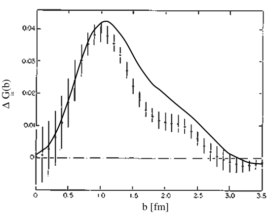
Figure 1: The growth speed of the inelastic overlap integral $G_{in}({\bf b})$ as function of the impact parameter as obtained in [6] compared with the result of the simplified analysis in which the integration over $|t|$ is carried over up to $|t|=1.0$ GeV² (see text).

The most prominent feature is the drop of the blackness growth speed at the center $(b=0)$ which is, for very central collisions, even compatible with zero. This seems to indicate that the corresponding profile functions are already approaching the unitarity limit and therefore cannot grow arbitrarily in the center. The main contribution to the growth of the total cross section comes from a region of $\sim 1$ fm which lies at the periphery of the proton.

The ingredients which are necessary for this analysis are data with: a) high statistics in $t$ in order to obtain an accurate profile function, b) different $s$ in order to obtain a reliable derivative (the low statistics in $s$ is responsible for the large error bars in Fig. 1) and c) knowledge of the real part of the scattering amplitude. In order to test the conditions necessary for the observation of the central slowdown which is interpreted as a sign for the unitarity limit, the analysis was redone using the data sets published in [7], neglecting the real part of the amlitude and using variations of the upper bound of the Fourier integral in Eq. (1) in order to test which range in $t$ an experiment should minimally cover in order to observe this effect. The result for the inelastic overlap integral is compared to the analysis in [6] in Fig. 1 and the result for the growth speed of the profile function $\Gamma$ is shown in Fig. 2.

Figure 2: The growth speed of the cross section as function of the impact parameter for different upper bounds in the Fourier integral (error bars have been suppressed).

It is obvious that the main signal, namely the drop of $\Delta\Gamma$ for small ${\bf b}$, is still observable in this simplified analysis in both $\Delta G_{in}({\bf b})$ and $\Delta\Gamma({\bf b})$, even if we lower the upper bound of the integration down to 0.64 GeV². This gives confidence that the application of the same simplified analysis to the case of single diffractive dissociation may also work and defines the range in $t$ which should be known experimentally in order to observe this effect as $|t_{max}|\sim 0.6$ GeV².

3 Single diffraction

Unfortunately, the data situation for the single diffraction process $pp\rightarrow pX$, where the final state has a proton and a kinematically separated hadronic state excluding the proton, is not satisfactory. Data have been taken at ISR for several values of $s$ [4]; if the dependence on the mass of the diffractively produced state $X$ is integrated out, only about 10 data points per set are available to describe $\frac{d\sigma}{dt}$, starting from $t\sim 0.2$ GeV². Since the low $t$ region where the cross section is large gives a dominant contribution in the Fourier integral (1) and the resolution in $t$ is not high, a sufficiently accurate analysis based on the measured data alone is not possible. The same is true for the more recent data obtained by UA4 [2, 3], UA8 [1] and CDF [5] for vastly different $s$. However, existing parameterizations of the data allow to create ’virtual’ data sets. In the impact parameter analysis of these virtual data sets, the unitarization prescription of the parameterizations can be tested.

An adequate description of the shape of the single diffractive differential cross section is given by Regge theory, although the normalization is suppressed at high energies relative to the Regge prediction (see [8]). Here the differential cross section is written as (see e.g. [9]):

$$\frac{d^{2}\sigma}{dtdM_{X}^{2}}=\sum_{i,j,k}\frac{\beta_{ik}(0)\beta_{il}(t)\beta_{jl}(t)g_{ijk}(t)}{16\pi s}\left(\frac{s}{M_{X}^{2}}\right)^{\alpha_{i}(t)+\alpha_{j}(t)}(M_{X}^{2})^{\alpha_{k}(0)},$$ (6)

where $i,j,k$ are all possible combinations of pomeron and other Regge trajectories, and $\beta_{ik}$ and $g_{ijk}$ the corresponding vertex functions. Assuming factorization in the sense that the process can be regarded in two steps, where in the first step the proton emits a pomeron which subsequently, in the second step, hits the other proton and forms a hadronic state $X$, the formula can be cast into the form

$$\frac{d^{2}\sigma}{dtd\xi}=F_{\mathcal{P}/p}(t,\xi)\cdot\sigma^{tot}_{\mathcal{P}p}(s^{\prime})=[K|F_{1}(t)|^{2}\xi^{1-2\cdot\alpha_{\mathcal{P}}(t)}]\sigma_{0}[(\xi s)^{\alpha_{\mathcal{P}}(0)-1}]+\text{Reggeon contributions}.$$ (7)

Here $\xi$ is the momentum fraction that the pomeron carries away from its parent proton, $s^{\prime}\equiv M_{X}^{2}\approx\xi s$, $\alpha_{\mathcal{P}}(t)$ is the pomeron trajectory, $F_{1}(t)$ is the standard Donnachie-Landshoff form factor [10] and $K$ is a normalization factor for the pomeron flux. Based on this expression, two different parameterizations have been proposed by Erhan and Schlein [11] and by Goulianos [12].

It is neither the aim of the present paper to dwell on details of each parameterization, such as background effects and possible modifications of the Regge trajectory, nor to compare their ability to reproduce the data. The focus is rather on a test of the different prescriptions used for unitarization of the total cross sections which can be calculated from the two parameterizations.

In the parameterization by Erhan and Schlein, unitarization is done via a modification of the pomeron trajectory (which is usually given as $\alpha_{\mathcal{P}}(t)=\alpha_{0}+\alpha^{\prime}\cdot t$). Here the trajectory acquires a term which is quadratic in $t$ (and unimportant for the purpose of the present analysis since it affects only the high $t$ range with $t>1$ GeV² to which this analysis is insensitive) and the parameters $\alpha_{0},\alpha^{\prime}$ and $\alpha^{\prime\prime}$ (here $\alpha^{\prime\prime}$ is the coefficient of the new quadratic term in the pomeron trajectory) are modified as a function of $s$ according to

$$\alpha_{0}(s)=\alpha_{0}(s_{0})+A\cdot\ln\left(\frac{s}{s_{0}}\right),\alpha^{\prime}(s)=\alpha^{\prime}(s_{0})+A^{\prime}\cdot\ln\left(\frac{s}{s_{0}}\right)\text{and}\quad\alpha^{\prime\prime}(s)=\alpha^{\prime\prime}(s_{0})+A^{\prime\prime}\cdot\ln\left(\frac{s}{s_{0}}\right).$$ (8)

For a negative value of $A$ this causes deviations from the power law and allows to fit the total cross section data.

On the other hand, in the parameterization by Goulianos a fundamentally different approach is used. Here, it is assumed as a working hypothesis that the pomeron flux $F_{\mathcal{P}/p}(t,\xi)$ from the parent proton cannot exceed unity. Therefore the factor $K$ in Eq. (7) is adjusted in such a way as to meet this condition. This results in a drastic change in the growth speed at some critical $s$ beyond which the growth of the total cross section is slowed down significantly.

It is evident that these two mechanisms to introduce unitarity into Eq. (7) are fundamentally different. Both of them are able to meet the unitarity condition imposed on the total cross section as seen from the present data. The critical question, which now arises, is the following: Since elastic scattering and single diffraction are both constrained by the same unitarity condition that (assuming negligible real part of the scattering amplitude) the probability for any interaction must be smaller than one at some given impact parameter, the same behaviour in the growth speed $\Delta\Gamma({\bf b})$ should be seen, namely a slowing down of central growth as compared to peripheral modes.

Figure 3: Profile functions obtained by the parameterizations by Erhan, Schlein and by the one of Goulianos for different values of $s$.

Figure 4: Impact parameter analysis of the growth speed $\Delta\Gamma$ based on the parameterization by Erhan and Schlein and the one by Goulianos in the ISR energy range (534 GeV${}^{2}\leq s\leq 3906$ GeV²). Shown for comparison is the result of the analysis of the elastic data as plotted in Fig. 2.

The actual analysis is done in a way similar to the one done in the elastic case. Data sets are created from the parameterizations at values of $s$ in the range of the ISR data, by integrating Eq. 7 over $\xi$ for fixed $t$. The lower limit of the $\xi$ integration is given by $s^{\prime}_{min}/s$ where $s^{\prime}_{min}$ corresponds to the lowest excited state of the proton and the upper limit is choosen in accordance with the experimental definition of the published $\frac{d\sigma}{dt}$ data sets as $\xi_{max}=0.05$. Both parametrizations have been used exactly as they appear in [11, 12], i.e. including reggeon contributions. These data sets are then treated as in the elastic case; the scattering amplitude is reconstructed assuming a vanishing real part and the profile function is calculated according to Eq. (1). Figure 3 shows the resulting profile functions and Fig. 4 shows the result of the growth speed analysis.

It is evident from the figure that a unitarization prescription such as the flux renormalization by Goulianos leads to a picture which is in better agreement with the one based on the elastic data. In that (dashed) curve, the dip for central collisions is at least indicated, whereas the other parameterization (by Erhan and Schlein) does not show any sign of a slower growth of the central blackness — quite the opposite is seen, in apparent contradiction to the (dotted) elastic result.

Figure 5: Impact parameter analysis of the growth speed $\Delta\Gamma$ based on the parameterization by Erhan and Schlein and the one by Goulianos in the energy range of the UA4 and UA8 [1, 2, 3] (540 GeV$<\sqrt{s}<$ 630 GeV) and the CDF measurements[5] ($\sqrt{s}=1800$ GeV).

The parameterizations can also be tested in the much higher energy range experimentally accessed by UA4 and UA8. The same analysis as above was made in the range 540 GeV $<\sqrt{s}<$ 630 GeV and the result is shown in Fig. 5. Here, the main features of the ISR energy result appear again, although somewhat more pronounced. This can also be seen in Fig. 3, where the profile functions of both parameterizations are similar at $s=550$ GeV, whereas the one by Erhan and Schlein exhibits a larger central growth than the one by Goulianos when compared at $\sqrt{s}=630$ GeV. This trend is confirmed looking at the $\sqrt{s}=1800$ GeV data obtained by CDF.

Let us conclude this section with a few critial remarks on the analysis and a summary of basic assumptions. First of all, the expression for the profile function, Eq. 1, is valid at asymptotic energies only. At finite energies, a mathematically correct treatment has been developed (see e.g.[13]) and, in principle, should be used. Next, throughout the analysis, the real part of the scattering amplitude has been neglected. This appears to be justified by looking at Fig. 1, where this approximation amounts only to a small difference for ISR energies. Similar assumptions are used in the standard analysis of high-energy elastic hadron scattering. The last issue concerns the form of the parametrizations used. Here, only one of the diagrams shown by Ross and Yam [14] has been used in both cases discussed in this paper. On the other hand, both parametrizations are able to account for the data where available. Clearly the shape of the profile functions resulting from the present analysis is central, in spite of the peripheral nature of diffraction. However, the conclusions concerning the unitarization of the parametrizations do not depend on the last two issues.

4 Summary

We have shown that the impact parameter analysis is a useful tool to investigate how effects caused by unitarity limits are distributed across the impact parameter space. The strongest manifestations of such effects should be found for central collision where the blackness is largest, resulting in a slowing down of the growth speed of the profile for small impact parameters. This method can not only be used for measured data but also in order to analyse unitarization prescriptions in empirical parameterizations. The reaction $pp\rightarrow pX$ has been considered here to demonstrate that unitarization by flux renormalization is closer to what one would expect, guided by the analysis of the elastic scattering data, than unitarization by introduction of an $s$-dependent pomeron intercept.

I thank G. Piller and W. Weise for helpful comments and discussions.

References

- [1] A. Brandt et al. (UA8 Collaboration), Nucl. Phys. B514, (1998) 3
- [2] M. Bozzo et al. (UA4 Collaboration), Phys. Lett. B 136 (1984) 217
- [3] M. Bernard et al. (UA4 Collaboration), Phys. Lett. B 186 (1987) 227
- [4] M. G. Albrow et al., Nucl. Phys. B 54 (1973) 6; M. G. Albrow et al., Nucl. Phys. B 72 (1974) 376
- [5] F. Abe et al. (CDF Collaboration), Phys. Rev. D50 (1994) 5535
- [6] U. Amaldi and K. R. Schubert, Nucl. Phys. B166 (1980) 301
- [7] K. R. Schubert, Tables on nucleon nucleon scattering, Landolt-Börnstein, 1/9A (1979)
- [8] K. Goulianos, Phys. Lett. B 358 (1995) 379
- [9] R. D. Field and G. C. Fox, Nucl. Phys. B 80 (1974) 367
- [10] A. Donnachie and P. V. Landshoff, Nucl. Phys. B 231 (1984) 189; A. Donnachie and P. V. Landshoff, Nucl. Phys. B 267 (1986) 690
- [11] S. Erhan and P. E. Schlein, Phys. Lett. B481 (2000) 177
- [12] K. Goulianos and J. Montanha, Phys. Rev. D59 (1999) 114017
- [13] T. Adachi and T. Kotani, Progr. Theor. Phys. Suppl., Extra Number (1965) 316; Progr. Theor. Phys. 35 (1966) 463; 36 (1966) 745; 37-38 (1966) 297
- [14] M. Ross and Y. Y. Yam, Phys. Rev. Lett. 19 (1967) 546