[

FZJ-IKP(TH)-2001-02
Chiral Lagrangians at finite density

Abstract

The effective $SU(2)$ chiral Lagrangian with external sources is given in the presence of non-vanishing nucleon densities by calculating the in-medium contributions of the chiral pion-nucleon Lagrangian. As a by product, a relativistic quantum field theory for Fermi many-particle systems at zero temperature is directly derived from relativistic quantum field theory with functional methods.

PACS numbers: 12.39.Fe, 24.85.+p, 13.75.L, 13.75.Gx

]

1. In the limit of massless up and down quarks the QCD Lagrangian is symmetric under the chiral group $SU(2)_{L}\times SU(2)_{R}$. One assumes that this symmetry is spontaneously broken to the diagonal subgroup $SU(2)_{L+R}$ giving rise to the appearance of 3 massless Goldstone bosons which finally acquire small masses due to the non-vanishing mass of the $u$ and $d$ quarks.

This symmetry breaking scenario constrains so much the interactions of the Goldstone bosons that the QCD Green functions can be calculated at low energies as an expansion in powers of momenta and quark masses. This is known as Chiral Perturbation Theory[1, 2].

The extension of the theory to the case of low temperature at zero density was considered in ref.[3]. In this article we study the case of small densities at zero temperature and derive the corresponding chiral Lagrangian by calculating the in-medium contributions due to the chiral pion-nucleon Lagrangian[4, 5] with functional methods. Although we focus our treatment to QCD, the relativistic many-body formalism here deduced for Fermi  systems can be applied to processes governed by other dynamical theories, as the traditional non-relativistic zero temperature many-body [6, 7] quantum theory which stresses the diagrammatic approach. Compared with standard quantum field theory at finite temperature $T$[8, 9] in the grand canonical ensemble, one avoids the use of unknown chemical potentials which themselves have to be calculated in terms of the many-body forces. The former is accomplished by following quantum field theory at $T=0$ considering directly the change of the ground state from the vacuum to one with finite fermionic densities. In the same way one also avoids the non-trivial $T\rightarrow 0$ limit due to the so called anomalous diagrams[10, 11]. The price to pay is to rely on the adiabatic hypothesis in order to determine the interacting ground state from that of the free case by turning on the interactions adiabatically.

2. Let us take first the case of symmetric and unpolarized nuclear matter, the extension of the formalism to the asymmetric and polarized case is straightforward and will be shown below. In the following we take the Heisenberg picture and, following closely scattering theory[13], we consider two ground states $|\Omega_{\hbox{out}}\rangle$ and $|\Omega_{\hbox{in}}\rangle$ which, under the action of any time dependent operator at asymptotic times $t\rightarrow\pm\infty$, respectively, behave as two symmetric Fermi seas of free protons and neutrons. The Fermi seas are filled up to the corresponding baryonic density, $\displaystyle{\prod^{N}}$$a^{\dagger}({\mathbb{p}}_{n})|0\rangle$, where the label $n$ includes also the spin and isospin indices, $N$ is the number of momentum states inside the Fermi sea with Fermi momentum $k_{F}=(3\pi^{2}\rho/2)^{1/3}$, $\rho$ is the total nuclear density and $|0\rangle$ is the vacuum. Our objective is to evaluate the generating functional ${\mathcal{Z}}[v,a,s,p]$ in the presence of vector $v_{\mu}$, axial $a_{\mu}$, scalar $s$ and pseudoscalar $p$ external fields[2] by working out the transition amplitude $\langle\Omega_{\hbox{out}}|\Omega_{\hbox{in}}\rangle_{J}$, where the label $J$ just indicates the presence of the aforementioned external sources. In this way by taking functional derivatives of ${\mathcal{Z}}[v,a,s,p]$ with respect to the external sources one evaluates the in-medium QCD connected Green functions (space-time averages at finite density of the quark currents coupled to the $v$, $a$, $s$ and $p$ sources). To do this we consider the effective chiral Lagrangians ${\cal L}={\cal L}_{\pi\pi}+{\cal L}_{\bar{\psi}\psi}+{\cal L}_{\bar{\psi}\psi\bar{\psi}\psi}+...$ with increasing number of pairs of nucleon fields $\psi(x)$. We first restrict ourselves to the term with no nucleon fields ${\cal L}_{\pi\pi}$ and to that containing two of them ${\cal L}_{\bar{\psi}\psi}=\bar{\psi}(x)D(x)\psi(x)$, together with the previous external fields. We will discuss later a way to include perturbatively the contributions of Lagrangians with higher number of nucleons by considering them to arise from bilinear vertices through the exchange of an arbitrary heavy particle. Indeed, although we are talking about CHPT, the only thing that matters for the following derivations is that ${\cal L}_{\bar{\psi}\psi}$ is bilinear in the fermions. Consider now the transition amplitude for the ground states from $t\rightarrow-\infty$ to $t\rightarrow+\infty$ in the presence of the previous external sources together with Grassmann sources $\eta$ and $\eta^{\dagger}$, coupled to the nucleon fields:

$$\langle\Omega_{\hbox{out}}|\Omega_{\hbox{in}}\rangle_{J,\eta,\eta^{\dagger}}=\!\int\![dU][d\psi][d\psi^{\dagger}]\langle\Omega_{\hbox{out}}|\psi(+\infty)\rangle\times$$ (1)

$$e {}^{i\!\int\!dx\left[{\mathcal{L}}_{\pi\pi}+\bar{\psi}D\psi+\eta^{\dagger}\psi+\psi^{\dagger}\eta\right]}\langle\psi(-\infty)|\Omega_{\hbox{in}}\rangle$$ (2)

with the pion fields described by the $2\times 2$ unitary matrix $U$.

The ground state functional $\langle\psi(\pm\infty)|\Omega_{{\begin{array}[]{c}\hbox{out}\\ \hbox{in}\end{array}}}\rangle$ can be expressed in terms of that of the vacuum by writing the $a(\mathbb{p}_{n})_{\!\!{\begin{array}[]{c}\hbox{out}\\ \hbox{in}\end{array}}}$ operators as a function of $\psi(x)$ and its time derivative $\dot{\psi}(x)$:

$$a({\mathbb{p}}_{n})_{\!\!{\begin{array}[]{c}\hbox{out}\\ \hbox{in}\end{array}}}\!=\!\lim_{{t\rightarrow\pm\infty}}\frac{E(p)}{2m_{N}}e^{iE(p)t}\!\int\!d{\mathbb{x}}\,e^{-i{\mathbb{p}}{\mathbb{x}}}\bar{u}({\mathbb{p}}_{n})[\psi_{n}(x)$$ (5)

$$+\frac{i}{E(p)}\dot{\psi}_{n}(x)],$$ (6)

where as usual in scattering theory for $t\rightarrow\pm\infty$ the matrix elements are calculated as if there were no interactions. In the former expression, $E(p)$ is the energy of the nucleon with three-momentum ${\mathbb{p}}$, $m_{N}$ is the nucleon mass and $u({\mathbb{p}}_{n})$ is a Dirac spinor. Expressing $\dot{\psi}(x)$ in terms of $\psi(x)$ (one way is using the Dirac equation), taking into account that $\psi(x)e^{i\!\int\!dy\,\eta^{\dagger}(y)\psi(y)}=-i\frac{\stackrel{{\scriptstyle\rightarrow}}{{\delta}}}{\delta\eta^{\dagger}(x)}e^{i\!\int\!dy\,\eta^{\dagger}(y)\psi(y)}$, the analogous expression for $\psi^{\dagger}(x)$, and substituting all that in eq.(1), one obtains for $\langle\Omega_{\hbox{out}}|\Omega_{\hbox{in}}\rangle_{J,\eta,\eta^{\dagger}}$:

$$\lim_{{\begin{array}[]{c}t\rightarrow+\infty\\ t^{\prime}\rightarrow-\infty\end{array}}}\!\int\e^{i\!\int\!dx{\cal L}_{\pi\pi}}\left(\prod_{n}^{N}\frac{E(p_{n})}{2m_{N}}\!\int\!d{\mathbb{x}}_{n}\,e^{ip_{n}x_{n}}\right.$$ (13)

$$\left.\bar{u}({\mathbb{p}}_{n})\bigg{[}1-\frac{i}{E(p_{n})}(\gamma^{0}\sum_{j=1}^{3}\gamma^{j}\frac{\partial}{\partial x_{n}^{j}}+i\gamma^{0}m_{N})\bigg{]}\frac{\stackrel{{\scriptstyle\rightarrow}}{{\delta}}}{\delta\eta^{\dagger}(x_{n})}\right)$$

$$e^{-i\!\int\!dx\!\int\!dy\,\eta^{\dagger}(x)D^{-1}(x,y)\gamma^{0}\eta(y)}\prod_{m}^{N}\frac{E(q_{m})}{2m_{N}}\!\int\!d{\mathbb{y}}_{m}\,e^{-iq_{m}y_{m}}$$

$$\Bigg{[}\frac{\stackrel{{\scriptstyle\leftarrow}}{{\delta}}}{\delta\eta(y_{m})}-\frac{i}{E(q_{m})}\bigg{(}\sum_{k=1}^{3}\frac{\partial}{\partial y_{m}^{k}}\frac{\stackrel{{\scriptstyle\leftarrow}}{{\delta}}}{\delta\eta(y_{m})}\gamma^{k}\gamma^{0}+i\frac{\stackrel{{\scriptstyle\leftarrow}}{{\delta}}}{\delta\eta(y_{m})}$$

$$\gamma^{0}m_{N}\bigg{)}\Bigg{]}\gamma^{0}\,u({\mathbb{q}}_{m})$$

where the integration over the nucleon fields and conjugate momenta is also done. Furthermore we define $x_{n}=(t,{\mathbb{x}}_{n})$, $y_{m}=(t^{\prime},{\mathbb{y}}_{m})$, $p_{n}=(E(p_{n}),{\mathbb{p}}_{n})$ and analogously for $q_{m}$. The action of the spatial derivatives can be readily taken into account by integrating by parts. In this way, they only act on the corresponding exponentials giving rise to three-momenta factors that can be further simplified by applying the Dirac equation on the Dirac spinors. In this way we have:

$$\bar{u}({\mathbb{p}}_{n})\left[1-\sum_{j=1}^{3}\frac{p_{n}^{j}}{E(p_{n})}\gamma^{0}\gamma_{j}+\frac{m_{N}}{E(p_{n})}\gamma^{0}\right] = \frac{2m_{N}}{E(p)}u^{\dagger}({\mathbb{p}}_{n})$$ (14)

$$\left[1-\sum_{j=1}^{3}\frac{p_{n}^{j}}{E(p_{n})}\gamma^{0}\gamma_{j}+\frac{m_{N}}{E(p_{n})}\gamma^{0}\right]\gamma^{0}u({\mathbb{p}}_{n}) = \frac{2m_{N}}{E(p)}u({\mathbb{p}}_{n})$$ (15)

Applying the previous results to eq.(13) it simplifies to:

$$\lim_{{\begin{array}[]{c}t\rightarrow+\infty\\ t^{\prime}\rightarrow-\infty\end{array}}}\!\int\e^{i\!\int\!dx{\cal L}_{\pi\pi}}\bigg{(}\prod_{n}^{N}\!\int\!d{\mathbb{x}}_{n}\,e^{ip_{n}x_{n}}u^{\dagger}({\mathbb{p}}_{n})$$ (18)

$$\frac{\stackrel{{\scriptstyle\rightarrow}}{{\delta}}}{\delta\eta^{\dagger}(x_{n})}\bigg{)}\,e^{-i\!\int\!dx\!\int\!dy\,\eta^{\dagger}(x)D^{-1}(x,y)\gamma^{0}\eta(y)}\,\prod_{m}^{N}\!\int\!d{\mathbb{y}}_{m}e^{-iq_{m}y_{m}}$$ (19)

$$\frac{\stackrel{{\scriptstyle\leftarrow}}{{\delta}}}{\delta\eta(y_{m})}u({\mathbb{q}}_{m})$$ (20)

After acting with the left derivatives $\stackrel{{\scriptstyle\rightarrow}}{{\delta}}\!\!/\delta\eta^{\dagger}(x_{n})$ on the exponential depending on the Grassmann sources, the former expression can be recast as:

$$\lim_{{\begin{array}[]{c}t\rightarrow+\infty\\ t^{\prime}\rightarrow-\infty\end{array}}}\!\int\e^{i\!\int\!dx{\cal L}_{\pi\pi}}\bigg{(}\prod_{n}^{N}\!\int\!d{\mathbb{x}}_{n}\,e^{ip_{n}x_{n}}\!\int\!dz_{n^{\prime}}$$ (23)

$$u^{\dagger}({\mathbb{p}}_{n})D^{-1}(x_{n},z_{n^{\prime}})\gamma^{0}\eta(z_{n^{\prime}})\bigg{)}e^{-i\!\int\!dx\!\int\!dy\,\eta^{\dagger}(x)D^{-1}(x,y)\gamma^{0}\eta(y)}$$ (24)

$$\prod_{m}^{N}\!\int\!d{\mathbb{y}}_{m}e^{-iq_{m}y_{m}}\frac{\stackrel{{\scriptstyle\leftarrow}}{{\delta}}}{\delta\eta(y_{m})}u({\mathbb{q}}_{m}).$$ (25)

This result is equal to $e^{i{\cal Z}[v,a,s,p]}$ when $\eta\rightarrow 0$ and $\eta^{\dagger}\rightarrow 0$. Hence we can equalize to 1 the second exponential from the left and the remaining right derivatives and $\eta(z_{n})$ sources have to be paired in order to finish with a non-vanishing result. Thus we have:

$$e^{i{\cal Z}}=\lim_{{\begin{array}[]{c}t\rightarrow+\infty\\ t^{\prime}\rightarrow-\infty\end{array}}}\!\int\e^{i\!\int\!dx{\cal L}_{\pi\pi}}\sum_{\sigma}\epsilon(\sigma)\prod_{n}^{N}\!\int\!d{\mathbb{x}}_{n}$$ (28)

$$\!\int\!d{\mathbb{x}}_{\sigma_{n}}\,e^{ip_{n}x_{n}}u^{\dagger}({\mathbb{p}}_{n})D^{-1}(x_{n},x_{\sigma_{n}})\gamma^{0}e^{-ip_{\sigma_{n}}x_{\sigma_{n}}}u({\mathbb{p}}_{\sigma_{n}})$$ (29)

with $\epsilon(\sigma)$ the signature of the permutation $\sigma$ over all the indices –momenta, spin and isospin. In order to continue let us write the operator $D(x)\equiv D_{0}(x)-A(x)$ with $D_{0}(x)=i\gamma^{\mu}\partial_{\mu}-m_{N}$ the Dirac operator for the free motion of the nucleons. On the other hand, the operator $A(x)$ is completely general although in our case at hand, CHPT, it is subject to a chiral expansion of powers of soft three-momenta and quark masses. Furthermore, let us note that:

$$\lim_{t\rightarrow+\infty}\!\int\!d{\mathbb{x}}\,e^{ipx}u^{\dagger}({\mathbb{p}})D_{0}^{-1}(x,x^{\prime})=-i\,e^{ipx^{\prime}}\bar{u}({\mathbb{p}})$$ (30)

$$\lim_{t\rightarrow-\infty}\!\int\!d{\mathbb{x}}\,D^{-1}_{0}(x^{\prime},x)\gamma^{0}e^{-ipx}u({\mathbb{p}})=-i\,e^{-ipx^{\prime}}u({\mathbb{p}})$$ (31)

This result can be easily obtained by writing $D_{0}^{-1}(x,x^{\prime})$ in four-momentum space and then performing the integral over the temporal component of the momentum taking care of the imposed limits. For instance, let us take the first of the previous equations. Then we have:

$$\lim_{t\rightarrow+\infty}\!\int\!d{\mathbb{x}}\,e^{ipx}u^{\dagger}({\mathbb{p}})D_{0}^{-1}(x,x^{\prime})=$$ (32)

$$\lim_{t\rightarrow+\infty}\!\int\!d{\mathbb{x}}\,e^{ipx}u^{\dagger}({\mathbb{p}})\int\!\!\frac{dR}{(2\pi)^{4}}\frac{e^{-iR(x-x^{\prime})}(\not\mathrel{R}+m_{N})}{R^{2}-m_{N}^{2}+i\epsilon},$$ (33)

with $\epsilon$ a positive infinitesimal. Exchanging the order of the integrations, the spatial one gives rise to $(2\pi)^{3}\delta({\mathbb{R}}-{\mathbb{p}})$ which fixes ${\mathbb{R}}$. As a result one has:

$$\lim_{t\rightarrow+\infty}\!\int\!\frac{dR^{0}}{2\pi}u^{\dagger}({\mathbb{p}})\frac{e^{ip^{0}t}e^{-iR^{0}(t-x^{\prime}_{0})}e^{-i{\mathbb{p}}{\mathbb{x}}^{\prime}}}{R_{0}^{2}-{\mathbb{p}}^{2}-m_{N}^{2}+i\epsilon}\!\!\left(R^{0}\gamma^{0}\!-\!{\mathbb{p}}{\mathbb{\gamma}}+m_{N}\right)$$ (34)

Since $t\rightarrow+\infty$ then $t-x^{\prime}_{0}>0$ and we close the integration contour over $R^{0}$ with a semi-circle of infinite radius on the lower half-plane picking up the pole at $R^{0}=p^{0}-i\epsilon=E(p)-i\epsilon$. Applying the Dirac equation to the result one arrives to eq.(30).

Then taking into account eq.(30) and the expansion $D^{-1}\gamma^{0}=[D_{0}-A]^{-1}\gamma^{0}=D_{0}^{-1}\gamma^{0}+D_{0}^{-1}AD_{0}^{-1}\gamma^{0}+...$, we can rewrite eq.(28) as:

$$e^{i{\cal Z}}=\!\int\\,e^{i\!\int\!dx{\cal L}_{\pi\pi}}\sum_{\sigma}\epsilon(\sigma)\prod_{n}^{N}\!\int\!d{\mathbb{x}}_{n}\!\int\!d{\mathbb{x}}_{\sigma_{n}}$$ (35)

$$e^{-i{\mathbb{p}}_{n}{\mathbb{x}}_{n}}u^{\dagger}({\mathbb{p}}_{n})\Bigg{[}\delta({\mathbb{x}}_{n}-{\mathbb{x}}_{\sigma_{n}})\delta_{n,\sigma_{n}}-i\!\int\!dt\!\int\!dt^{\prime}\,e^{iE(p_{n})t}\gamma^{0}$$ (36)

$$A(x_{n},x_{\sigma_{n}})\,e^{-iE(p_{\sigma_{n}})t^{\prime}}-i\!\int\!dt\!\int\!dt^{\prime}\!\int\!dz\,dz^{\prime}\,e^{iE(p_{n})t}\gamma^{0}$$ (37)

$$A(x_{n},z)D_{0}^{-1}(z,z^{\prime})A(z^{\prime},x_{\sigma_{n}})e^{-iE(p_{\sigma_{n}})t^{\prime}}+...\Bigg{]}$$ (38)

$$\,e^{i{\mathbb{p}}_{\sigma_{n}}{\mathbb{x}}_{\sigma_{n}}}u({\mathbb{p}}_{\sigma_{n}})$$ (39)

where now both $t$ and $t^{\prime}$ are integration variables being the time components of $x_{n}$ and $x_{\sigma_{n}}$, respectively. The dots just refer to those terms with an increasing number of insertions of the operator $A$ coming from the geometric expansion of $D^{-1}=\left[D_{0}-A\right]^{-1}$ discussed above. Furthermore $A(x,y)$ is defined such that

$$\int dx\,\bar{\psi}(x)A(x)\psi(x)\!=\!\int\!dx\,dy\,\bar{\psi}(x)A(x,y)\psi(y).$$ (40)

As a result of eq.(35) we can simply state that:

$$e^{i{\cal Z}[v,a,s,p]}=\!\int\\,e^{i\!\int\!dx{\cal L}_{\pi\pi}}\,(\widetilde{\hbox{det}}\,{\cal{F}})$$ (41)

where the tilde in $\widetilde{\hbox{det}}\,{{\cal F}}$ indicates that the determinant has to be taken in the subspace of the Fermi sea states expanded by the basis functions $e^{i{\mathbb{p}}_{n}{\mathbb{x}}}u({\mathbb{p}}_{n})$ with $|{\mathbb{p}}_{n}|<k_{F}$. In this notation ${\cal F}$ is given by:

$${\cal F}\equiv I_{3}-i\!\int\!dt\!\int\!dt^{\prime}\,e^{iH_{0}t}\,\gamma^{0}A\left[I_{4}-D^{-1}_{0}A\right]^{-1}\,e^{-iH_{0}t^{\prime}}$$ (42)

where $I_{3}\equiv\delta({\mathbb{x}}_{n}-{\mathbb{x}}_{m})\delta_{n,m}$ and analogously $I_{4}\equiv\delta(x_{n}-x_{m})\delta_{n,m}$. On the other hand, $e^{-iH_{0}t^{\prime}}e^{i{\mathbb{p}}_{n}{\mathbb{x}}^{\prime}}u({\mathbb{p}}_{n})=e^{-ip_{n}x^{\prime}}u({\mathbb{p}}_{n})$ and $e^{-i{\mathbb{p}}_{n}{\mathbb{x}}}u^{\dagger}({\mathbb{p}}_{n})e^{iH_{0}t}=e^{ip_{n}x}u^{\dagger}({\mathbb{p}}_{n})$.

In order to obtain from eq.(41) the contributions of the surrounding medium to the generating functional it is convenient to exponentiate $\widetilde{\hbox{det}}\,{\cal F}$ as $\exp(\widetilde{\hbox{Tr}}\log{\cal F})$ (where the tilde has the same meaning as before). Then we have:

$$e^{i{\cal Z}[v,a,s,p]}=\!\int\\exp\bigg{\{}i\!\int\!dx{\cal L}_{\pi\pi}+\sum_{r=1}^{2}\sum_{\alpha=1}^{2}$$ (43)

$$\!\int^{k_{F}}\frac{d{\mathbb{p}}}{(2\pi)^{3}2E(p)}\!\int\!d{\mathbb{x}}\!\int\!d{\mathbb{y}}\,e^{-i{\mathbb{p}}{\mathbb{x}}}u^{\dagger}_{r\alpha}({\mathbb{p}})\,\log[{\cal F}]\arrowvert_{({\mathbb{x}}\,\alpha,{\mathbb{y}}\,\alpha)}$$ (44)

$$\,e^{i{\mathbb{p}}{\mathbb{y}}}u_{r\alpha}({\mathbb{p}})\bigg{\}}$$ (45)

where we have indicated explicitly the spin $r$ and isospin $\alpha$ indices. It is very appropriate to stress at this point that eq.(43), although formal, is non-perturbative. From this result we can readily read out the new effective chiral Lagrangian density $\tilde{{\cal L}}_{\pi\pi}$ in the presence of a nuclear density just by equating the expression between curly brackets to $i\!\int\!dx\,\tilde{{\cal L}}_{\pi\pi}$.

3. The perturbative theory is obtained by expanding $\log{\cal F}$ in eq.(43), so that $e^{i{{\cal Z}}}$ can be written as:

$$\!\int\\exp\Bigg{\{}i\!\int\!dx\,{\cal L}_{\pi\pi}-i\sum_{r=1}^{2}\sum_{\alpha=1}^{2}\!\int^{k_{F}}\frac{d{\mathbb{p}}}{(2\pi)^{3}2E(p)}$$ (46)

$$\!\int\!dx\,dy\,e^{ipx}\bar{u}_{r\alpha}({\mathbb{p}})\,A[I_{4}-D^{-1}_{0}A]^{-1}\arrowvert_{(x\alpha,y\alpha)}\,e^{-ipy}u_{r\alpha}({\mathbb{p}})$$ (47)

$$+\frac{1}{2}\sum_{r,s=1}^{2}\sum_{\alpha,\beta=1}^{2}\!\int^{k_{F}}\frac{d{\mathbb{p}}}{(2\pi)^{3}2E(p)}\!\int^{k_{F}}\frac{d{\mathbb{q}}}{(2\pi)^{3}2E(q)}\!\int\!dx\,dx^{\prime}\,dy^{\prime}\,dy$$ (48)

$$e^{ipx}\bar{u}_{r\alpha}({\mathbb{p}})\,A[I_{4}-D_{0}^{-1}A]^{-1}\arrowvert_{(x\alpha,x^{\prime}\beta)}\,e^{-iqx^{\prime}}u_{s\beta}({\mathbb{q}})\,e^{iqy^{\prime}}\bar{u}_{s\beta}({\mathbb{q}})$$ (49)

$$A[I_{4}-D_{0}^{-1}A]^{-1}\arrowvert_{(y^{\prime}\beta,y\alpha)}\,e^{-ipy}u_{r\alpha}({\mathbb{p}})+...\Bigg{\}}.$$ (50)

Finally, taking into account the relation $\displaystyle{\sum_{r=1}^{2}}$$u_{r}({\mathbb{p}})\otimes\bar{u}_{r}({\mathbb{p}})=\not\mathrel{p}+m_{N}$ we arrive at the following expression for the generating functional:

$$e^{i{\cal Z}}=\!\int\\exp\Bigg{\{}i\!\int\!dx\,{\cal L}_{\pi\pi}-i\!\int^{k_{F}}\frac{d{\mathbb{p}}}{(2\pi)^{3}2E(p)}$$ (51)

$$\!\int\!dx\,dy\,e^{ip(x-y)}\,\hbox{Tr}\Bigg{(}A[I_{4}-D_{0}^{-1}A]^{-1}\arrowvert_{(x,y)}(\not\mathrel{p}+m_{N})\Bigg{)}+$$ (52)

$$\frac{1}{2}\!\int^{k_{F}}\frac{d{\mathbb{p}}}{(2\pi)^{3}2E(p)}\!\int^{k_{F}}\frac{d{\mathbb{q}}}{(2\pi)^{3}2E(q)}\!\int\!dx\,dx^{\prime}\,dy\,dy^{\prime}\,e^{ip(x-y)}$$ (53)

$$e^{-iq(x^{\prime}-y^{\prime})}\,\hbox{Tr}\Bigg{(}A[I_{4}-D_{0}^{-1}A]^{-1}\arrowvert_{(x,x^{\prime})}(\not\mathrel{q}+m_{N})A[I_{4}-$$ (54)

$$D_{0}^{-1}A]^{-1}\arrowvert_{(y^{\prime},y)}(\not\mathrel{p}+m_{N})\Bigg{)}+...\Bigg{\}}$$ (55)

where the trace refers both to the isospin and spinor indices. The previous formula implies a double expansion for obtaining the contributions of the nuclear medium to the chiral Lagrangian. One is the standard chiral expansion by expanding the vacuum operator $A[I_{4}-D_{0}^{-1}A]^{-1}=A+AD_{0}^{-1}A+AD_{0}^{-1}AD_{0}^{-1}A+...$ together with $A$ itself, $A=A^{(1)}+A^{(2)}+A^{(3)}+...$ in increasing powers of momenta and quark masses valid at low energies. Explicit expressions of $A$ up to ${\mathcal{O}}(p^{3})$ can be obtained from ref.[5]. 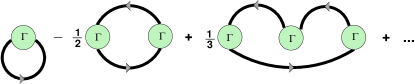The another is an expansion in the number of insertions of on-shell fermions belonging to the Fermi sea, schematically indicated in fig.1 by a thick solid line. Both expansions can be related by giving a chiral power couting to $k_{F}$ which can be naturally counted as ${\mathcal{O}}(p)$[14] since for nuclear saturation density $k_{F}\simeq 2M_{\pi}$ with $M_{\pi}$ the pion mass. Moreover, the circles labeled by $\Gamma$ correspond to the non-local operator $-iA[I_{4}-D_{0}^{-1}A]^{-1}$. Note that when inserting $n$ Fermi seas from the expansion of the logarithm one picks up a factor $-(-1)^{n}/n$ where the global minus sign appears due to the fermionic closed loop, $n$ is a combinatoric factor because any cyclic permutation in the trace of $n$ Fermi seas with their associated $n$ $\Gamma$ operators gives the same result and finally the sign $(-1)^{n}$ is a pure in-medium factor that one has to keep in mind and is already present in standard many-body theory[7].

FIG. 1.: Diagrammatic expansion of eq.(51). Every thick line corresponds to the insertion of a Fermi-sea and each circle to the insertion of an operator $\Gamma\equiv-iA\left[I_{4}-D_{0}^{-1}A\right]^{-1}$.

A generally non-local vertex $\Gamma$ comes from the iteration of the $A$ operator with intermmediate free baryon propagators $D_{0}^{-1}$, obeying the usual Feynman rules, see fig.2. Notice that $A$ was defined from the Lagrangain $\bar{\psi}D\psi$ removing the free term $\bar{\psi}D_{0}\psi$ and changing the sign to the rest, this is why a minus sign appears in front of $A$ in fig.2. On the other hand $i\,D_{0}^{-1}(x,y)=i\,\int\frac{d^{4}p}{(2\pi)^{4}}\frac{\not\mathrel{p}+m_{N}}{p^{2}-m_{N}^{2}+i\epsilon}$ is the usual baryon propagator.

FIG. 2.: Expansion of the generalized non-local vacuum vertex $\Gamma$. Every solid line corresponds to a vacuum baryon propagator and each circle to the insertion of an operator $-iA$ from $\bar{\psi}D\psi$.

Hence a final diagram, when expanding $\Gamma$ up to the required accuracy, will be a set of $n\geq 1$ Fermi-sea insertions, $m\geq 0$ free baryon-propagators and of $m+n$ vertices $-iA$. First we include the $-1$ global sign because of the fermionic closed loop, and the combinatoric factor $1/n$ together with the sign $(-1)^{n}$. Then, following the diagram in the opposite sense to that of the fermionic arrows, write for each Fermi-sea an integral $\int^{k_{F}}\!\!\frac{d{\mathbb{p}}\,(\not\mathrel{p}+m)}{(2\pi)^{3}2E(p)}$ with $p^{0}=E(\mathbb{p})$, for each vaccum baryon propagator with free momentum $p$ write $i\int\!\!\frac{dp}{(2\pi)^{4}}\frac{\not\mathrel{p}+m_{N}}{p^{2}-m_{N}^{2}+i\epsilon}$ and for a vertex in momentum space a term $-iA(2\pi)^{4}$, keeping in mind the energy-momentum conservation at each vertex. Finally sum over the spin and isospin indices of the fermions. This defines explicitely the Feyman rules in momentum space in order to obtain $i(2\pi)^{4}$ times the desired connected graph accompied by the global delta of energy-momentum conservation. Analogous Feynman rules hold of course in configuration space, e.g., see eq.(51).

An equivalent way to state the previous rules, without including explicitely the integral symbols and factors $2\pi$, is to write the same sign-combinatoric factor $-(-1)^{n}/n$ and vertices $-iA$ as before. Then for the free nucleons one has just the free propagator $i\frac{\not\mathrel{p}+m}{p^{2}-m^{2}+i\epsilon}$ and for the Fermi-sea baryons the factor $(2\pi)\delta(p^{2}-m^{2})\theta(p^{0})(\not\mathrel{p}+m)\theta(k_{F}-|\mathbb{p}|)$. Finally sum over all the discrete indices attached to the fermions and integrate over all the free four-momenta with the measure $\int d^{4}p/(2\pi)^{4}$ after taking into account energy-momentum conservation at each vertex.

Fig.1 fixes the skeleton structure of standard in-medium vertices since still one has to consider the pion fields contained in $A$ over which one has to integrate in eqs.(43), (51) to finally obtain the generating functional. That is, from the vertices $A$ as well as from ${\cal L}_{\pi\pi}$, one can generate internal as well as external (coupled to the sources) pionic legs denoted by dashed lines in figs.3a and 3b. Here one has essentially the same Feynamn rules than in vaccum in order to proceed in a perturbative way, simply for each pionic line with four-momentum $q$, one writes the vacuum propagator $i\int\frac{dq}{(2\pi)^{4}}\frac{1}{q^{2}-M_{\pi}^{2}+i\epsilon}$, for the first version of the in-medium Feynman rules. For the second one has $\frac{i}{q^{2}-M_{\pi}^{2}+i\epsilon}$. The important remark to keep in mind is that a generalized vertex has analogous properties to those of a standard local quantum field theory one to the effects of determing the numerical factors accompanying the exchange of pion lines inside a given diagram. This can be seen just by applying standard perturbative techniques in path integrals to the action given between brackets in eq.(43) or more explicitely in eq.(51). Several examples are discussed in detail in ref.[14].

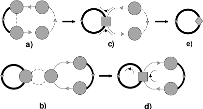
4. Notice also that ultra-violet parts in the integration over running pionic momenta generate local multi-nucleon vertices and hence a proper treatment of pion loops can only be done by including simultaneously local nucleon interactions in order to reabsorb the divergences. This is denoted by the squares in figs. 3c and 3d. It is important to realize that while in fig.3a the pion is exchanged inside the same vertex (in the generalized sense of above) in fig.3b the pions are exchanged between two of them. This implies the presence of only one Dirac trace in fig.3c (the flow of the Dirac indices along the propagators on both sides of the square is indicated by the arrows of the open solid lines) and two Dirac traces in fig.3d. Thus, when writing the matrix elements corresponding to diagrams of the type of figs.3c and 3d (with local interactions) one has to keep track of the number of closed traces in the spinor indices since each of them will lead to a sign $(-1)$ and its own combinatoric factor $1/n_{j}$ (with $n_{j}$ the number of Fermi-sea insertions in the closed Dirac loop) together with the sign $(-1)^{n_{j}}$. One can also arrive to the same conclusions by considering that the dashed lines originate from the exchange of an arbitrary heavy meson (the only relevant point in our derivations is the bilinear character of the meson-$\bar{N}N$ interaction in the nucleon fields). In this way it is straightforward to realize the presence of a factor $1/2$ in front of fig.3d together with the factors $\prod_{j}(-1)^{n_{j}+1}/n_{j}$ which here is simply $1$. The relation between contact four nucleon interactions at low energies in effective field theories and its saturation by integrating-out heavy meson resonances has been established in ref.[15].

FIG. 3.: Diagrams 3a and 3b represent some typical many-particle diagrams generated from eqs.(43), (51). The circle indicates an $A$ operator insertion (which in addition can have attached to it more lines than shown) and the dashed line corresponds to a pion exchange. Figs.3c and 3d arise by considering the ultra-vioalet divergent part of the pion loops leading to local terms denoted by squares. Fig.3e is a local $\pi N$ counterterm, indicated by a diamond. For more details see the text.

There is still an important difference to be discussed when comparing figs.3c and 3d, which in fact is related to the presence of the factor (det$\,D$) in all the formulae from eq.(13) to eq.(51). The latter corresponds to contributions to the chiral Lagragian from closed fermion loops in the vacuum and in the spirit of the effective field theories these contributions, coming from states with masses close to or above the chiral scale $\Lambda_{\chi}\approx M_{\rho}$, are incorporated in the counterterms of the vacuum effectrive field theory. In this way we will set det$\,D=1$ in the following. Indeed on the right hand side of the square of fig.3c we can recognize a momentum loop flowing along the free baryon propagators without any insertion of a Fermi-sea. This simply means that since all the momenta that could go into this closed momentum loop are soft because they come from the circles, it just corresponds to vacuum renormalization from heavy particles and is reabsorbed in the low energy counterterms. This is schematically shown in fig.3e with a diamond corresponding to a higher order $\pi N$ counterterm. This is consistent as far as one is restricted to the low energy and momentum regime. However, when a Fermi-sea baryon line is present the momentum running though the baryon lines is of the form $p_{j}=p+Q_{j}$ with $p=(E(p),\mathbb{p})$ and $|{\mathbb{p}}|<k_{F}$. Thus one is inserting a medium parameter $k_{F}$ and shifting upward up to around $m_{N}$ the energy level around which one is perturbating.

5. We now turn to the generalization of the formalism to the case of asymmetric nuclear matter, with different densities of neutrons, $\rho_{n}$, and protons, $\rho_{p}$, with Fermi momenta $k_{F}^{(n)}=(3\pi^{2}\rho_{n})^{1/3}$ and $k_{F}^{(p)}=(3\pi^{2}\rho_{p})^{1/3}$, respectively. Following the previous derivation of eq.(43) one can easily convince oneself that the only change is to remove the sum over isospin indices and to distinguish between $\alpha=1$ (proton) and $\alpha=2$ (neutron). In this way we will have:

$$e^{i{\cal Z}[v,a,s,p]}=\!\int\![dU]\exp\Bigg{\{}i\!\int\!dx{\cal L}_{\pi\pi}+\sum_{r=1}^{2}$$ (56)

$$\!\int^{k_{F}^{(p)}}\frac{d{\mathbb{p}}}{(2\pi)^{3}2E(p)_{1}}\!\int\!d{\mathbb{x}}\!\int\!d{\mathbb{y}}e^{-i{\mathbb{p}}{\mathbb{x}}}u^{\dagger}_{r\,1}({\mathbb{p}})\,\log[{\cal F}]\arrowvert_{({\mathbb{x}}\,1,{\mathbb{y}}\,1)}$$ (57)

$$e^{i{\mathbb{p}}{\mathbb{y}}}u_{r\,1}({\mathbb{p}})+\sum_{r=1}^{2}\!\int^{k_{F}^{(n)}}\frac{d{\mathbb{p}}}{(2\pi)^{3}2E(p)_{2}}\!\int\!d{\mathbb{x}}\!\int\!d{\mathbb{y}}\,e^{-i{\mathbb{p}}{\mathbb{x}}}$$ (58)

$$u^{\dagger}_{r\,2}({\mathbb{p}})\,\log[{\cal F}]\arrowvert_{({\mathbb{x}}\,2,{\mathbb{y}}\,2)}\,e^{i{\mathbb{p}}{\mathbb{y}}}u_{r\,2}({\mathbb{p}})\Bigg{\}}$$ (59)

Notice that we have indicated separately the energies of protons $E(p)_{1}$ and neutrons $E(p)_{2}$ with three-momentum ${\mathbb{p}}$, since the previous equation is valid for the non-isospin limit as well. Nevertheless, in order to simplify the formulae, we will consider in the following the case with equal nucleon masses. We also introduce the $2\times 2$ matrix:

$$n(p) = \left(\begin{array}[]{cc}\theta(k_{F}^{(p)}-p)&0\\ 0&\theta(k_{F}^{(n)}-p)\end{array}\right)$$ (62)

$$\equiv \left(\begin{array}[]{cc}n(p)_{1}&0\\ 0&n(p)_{2}\end{array}\right)$$ (65)

$$= \hat{n}(p)I_{2}+\bar{n}(p)\tau_{3}$$ (66)

with $I_{2}$ the $2\times 2$ unity matrix, $\tau_{3}$ the usual Pauli matrix $diag(1,-1)$, $\hat{n}(p)=(n(p)_{1}+n(p)_{2})/2$ and $\bar{n}(p)=(n(p)_{1}-n(p)_{2})/2$. Then eq.(56) can be rewritten as:

$$e^{i{\cal Z}[v,a,s,p]}=\!\int\![dU]\exp\bigg{\{}i\!\int\!dx{\cal L}_{\pi\pi}\!\!+\!\!\int\!\!d{\mathbb{x}}\!\!\int\!\!d{\mathbb{y}}\!\!\int\frac{d{\mathbb{p}}}{(2\pi)^{3}2E(p)}$$ (73)

$$e^{-i{\mathbb{p}}({\mathbb{x}}-{\mathbb{y}})}\hbox{Tr}\bigg{(}n(p)\log[{\cal F}]\arrowvert_{({\mathbb{x}},{\mathbb{y}})}(\not\mathrel{p}+m)\bigg{)}\bigg{\}}=$$

$$=\!\int\![dU]\exp\Bigg{\{}i\!\int\!dx\,{\cal L}_{\pi\pi}-i\!\int\!\frac{d{\mathbb{p}}}{(2\pi)^{3}2E(p)}\!\int\!dx\,dy\,e^{ip(x-y)}\,$$

$$\hbox{Tr}\Bigg{(}A[I_{4}-D_{0}^{-1}A]^{-1}\arrowvert_{(x,y)}(\not\mathrel{p}+m_{N})\,n(p)\Bigg{)}+$$

$$\frac{1}{2}\!\int\!\!\!\frac{d{\mathbb{p}}}{(2\pi)^{3}2E(p)}\!\int\!\!\!\frac{d{\mathbb{q}}}{(2\pi)^{3}2E(q)}\!\int\!dx\,dx^{\prime}\,dy\,dy^{\prime}\,e^{ip(x-y)}$$

$$e^{-iq(x^{\prime}-y^{\prime})}\,\hbox{Tr}\Bigg{(}A[I_{4}-D_{0}^{-1}A]^{-1}\arrowvert_{(x,x^{\prime})}\,(\not\mathrel{q}+m_{N})\,n(q)$$

$$A[I_{4}-D_{0}^{-1}A]^{-1}\arrowvert_{(y^{\prime},y)}(\not\mathrel{p}+m_{N})\,n(p)\Bigg{)}+...\Bigg{\}}.$$

Comparing this equation with eq.(51), the only difference in the Feynman rules is the inclusion of an isospin matrix $n(p)$ associated to every Fermi-sea insertion.

The case of a polarized nuclear matter can be treated in the same way just by doing in eq.(56) the replacement:

$$\sum_{r=1}^{2}\!\int^{k_{F}}d{\mathbb{p}}\,u^{\dagger}_{r\alpha}({\mathbb{p}})\;...\;u_{r\alpha}({\mathbb{p}})\rightarrow\!\int^{k_{F}}d{\mathbb{p}}\,u^{\dagger}_{r_{1}\alpha}({\mathbb{p}})\;...\;u_{r_{1}\alpha}({\mathbb{p}})$$ (74)

$$+\!\int^{k_{F}}d{\mathbb{p}}\,u^{\dagger}_{r_{2}\alpha}({\mathbb{p}})\;...\;u_{r_{2}\alpha}({\mathbb{p}})$$ (75)

since there are two spin states per momentum state.

6. The present formalism is applied in ref.[14] to evaluating several quantities relevant for low energy QCD in the nuclear medium. There we will also address in detail the issue of the chiral counting from eq.(73) in the nuclear medium and the limitations of a plain perturbative treatment of CHPT at finite density. Just to mention that instead of a relativistic treatment of the baryons we could also have considered in the same way the non-relativistic case. This makes more straightforward the evaluation of baryon loops [16] although one has also to take into account recent developments in the field of effective field theories with propagation of relativistic heavy particles [17, 18, 19]. In any case the main issue still to be addressed in the medium, as discussed in refs. [16, 14], is to deal with the problem of the large S-wave scattering lengths in the nucleon-nucleon scattering which introduces a new extra scale of only $\sim$10 MeV alredy in the vaccum case, where consistent power counting schemes have been developed[20]. Some interesting findings in this direction, requiring further consideration, can be found in ref.[21] for a theory without pions.

To conclude, we have derived the $SU(2)$ chiral Lagrangian with extenal sources in the presence of non-zero nuclear density by explicitely working out in quantum field theory the in-medium contributions from the $\pi N$ chiral Lagrangian, eq.(51)(symmetric nuclear matter), eq.(73) (asymmetric nuclear matter) and eq.(74) (asymmetric and unpolarized nuclear matter). Then the perturbative theory is developed and the corresponding Feynman rules are given. Contrarily to standard many-body techniques, the rules and diagrams here derived for the general relativistc case are analogous to the usual ones from vacuum quantum field theory without modification of the baryon propagators establishing a neat separation between in-medium and vacuum contributions, as indicated in figs.1 and 2. Applications of this many-particle relativistic quantum field theory formalism to actual calculations can be found in ref.[14].

I would like to thank Andreas Wirzba and Ulf-G. Meißner for useful discussions and for a critical reading of the manuscript. This work was supported in part by funds from DGICYT under contract PB96-0753 and from the EU TMR network Eurodaphne, contract no. ERBFMRX-CT98-0169.

REFERENCES

[1]S. Weinberg, Physica 96A, 327 (1979).
[2]J. Gasser and H. Leutwyler, Ann. Phys. (N.Y.) 158, 142 (1984).
[3]P. Binetruy and M.K. Gaillard, Phys. Rev. D32, 931 (1985);
J. Gasser and H. Leutwyler, Phys. Lett. B184, 83 (1987);
R.D. Pisarski and M. Tytgat, Phys. Rev. Lett. 78, 3622 (1997).
[4]J. Gasser, M.E. Sainio and A. Svarc, Nucl. Phys. B307,
779 (1988).
[5]N. Fettes, U.-G. Meißner and S. Steininger, Nucl. Phys.
A640, 199 (1998).
[6]The Quantum Theory of Many-Particle Systems, editor H.L. Morrison
(Gordon and Breach, Science Publisher, New York, 1962).
[7]A. L. Fetter and J. D. Walecka, Quantum Theory of Many-Particle
Systems, McGraw-Hill, New York, 1971.