Aspects of Non-Equilibrium Dynamics in Quantum Field Theory

Abstract

This work is devoted to the study of relaxation–dissipation processes in systems described by Quantum Field Theory. After a brief introduction to the main stream of applications and to the general CTP formalism, a preparatory study in quantum mechanics is presented.

I then introduce the scalar quantum field theory $\lambda\phi^{4}$ in finite volume, which is studied in the infinite $N$ limit, both at equilibrium and out of equilibrium. The dynamical equations are derived and solved numerically. I find that the zero-mode quantum fluctuations cannot grow macroscopically large starting from microscopic initial conditions. which leads to the conclusion that there is no evidence for a dynamical Bose-Einstein condensation, in the usual sense. On the other hand, out of equilibrium the long-wavelength fluctuations do scale with the linear size of the system, signalling dynamical infrared properties quite different from the equilibrium ones characteristic of the same approximation scheme.

With the aim of going beyond the gaussian approximation intrinsic in the large $N$ limit, I introduce a non-gaussian Hartree-Fock approximation (tdHF). I derive the mean-field coupled time-dependent Schroedinger equations for the modes of the scalar field and I renormalize them properly. The dynamical evolution in a further controlled gaussian approximation of our tdHF approach, for $N=1$, is studied from non-equilibrium initial conditions characterized by a uniform condensate. I find that, during the slow rolling down, the long-wavelength quantum fluctuations do not grow to a macroscopic size but do scale with the linear size of the system, as happens in the large $N$ approximation of the O(N) model. This behavior shows an internal inconsistency of this approximation. I also study the dynamics of the system in infinite volume with particular attention to the asymptotic evolution in the broken symmetry phase. We are able to show that the fixed points of the evolution cover at most the classically metastable part of the static effective potential.

Finally, the dynamical evolution in the $O(N+1)$ nonlinear sigma model in $1+1$ dimensions is investigated in the large N limit. I first of all verify that the large coupling limit of the $O(N+1)\,\phi^{4}$ model, which renders the model non linear, commutes with the large $N$ limit, so that the $O(\infty)$ nonlinear sigma model is uniquely defined. I then numerically study the evolution of several observables, with a particular attention to the spectrum of produced particles during the relaxation of an initial condensate and find no evidence for parametric resonance, a result that is consistent with the presence of the nonlinear contraint. Only a weak nonlinear resonance at late times is observed.

I conclude with some remarks on the “state of art” in gauge theories and some comments about the open issues in the subject.

Preface

This work is devoted to some aspects of the dynamical evolution in Quantum Field Theory (QFT). Before describing the specific attitude I will take and the applications I will be considering in the following chapters, I would like first to briefly introduce the general setting which the subject of this thesis belongs to and, at the same time, give at least one motivation to keep studying QFT.

If we go back in time and want to talk about the history of Theoretical Physics, few simple words might be enough: Unification of Concepts and Descriptions. If we look at the evolution of Theoretical Physics, starting from Newton’s theory of gravitation, up to the Standard Model of elementary interactions, passing through Maxwell’s electromagnetism, we realize that the dream of reducing the complexity of phenomena to a unique fundamental principle (or to the lowest number of them), has been one of the powerful and successful ideas, which have been leading theoretical physicists not only to describe in a simple and beautiful fashion the Nature as was known, but even to make important predictions and discoveries, later confirmed by the experiments [1, 2]. We might cite three great historical examples: the prediction of the existence of a new planet, Neptune, in the solar system (discovered later in 1846), according to the theory of gravitation and to the observational data on the orbits of the already known planets, the prediction of the Hertzian waves (experimentally observed in 1888), according to Maxwell’s theory of electromagnetism and the prediction of the existence of the electron’s antiparticle, the positron, according to the Dirac’s relativistic theory of the electron (discovered in 1932).

From this point of view, during the 20^th century, Theoretical Physics went very far on the path of Unification. The formulation of the Standard Model of the Electroweak Interactions, by S. Glashow, S. Weinberg and A. Salam [3, 4, 5] which worth the Nobel prize to its inventors, represents one of the brightest result of Theoretical Physics. Three of the four fundamental interactions of Nature, namely the electromagnetic, the weak and the strong forces, and all the phenomena which are related to them (almost the entire world as we know it), can be described in a single conceptual framework, using a unique “language” (as a side-product, again the $W$ and $Z$ vector bosons were predicted by the Standard Model before their discovery in 1983). This was possible thanks to the merging of two of the most important achievements of Theoretical Physics in the first half of XX^th century: Special Relativity [6] and Quantum Mechanics [7]. Since the first attempts to reconcile the two theories, it became evident that internal consistency asked for a Quantum Theory of Relativistic Fields to be formulated [8].

Then, in spite of the initial mistrust theoreticians devoted to QFT as the framework for a fundamental theory, the experiments has been showing at a deeper and deeper level the capability of such a “language” to describe with some simple words almost all the phenomena happening in our world (for completeness’ sake, I should say that this reductionist point of view may be applicable and justified when limited, for instance, to particle Physics, but its extension to the whole Physics, or the whole Science, has been deeply criticized [9]; for recent reviews and criticism of QFT, see also [10, 11, 12]) …

All but one. In fact, the gravitational interaction is still described by the Einstein’s General theory of Relativity (GR), which dates back to 1915 and is a classical (non-quantum) field theory. It is not the subject of this work to talk about the efforts made to include gravitation in a QFT description of Nature. Thus it will suffice to say that, even though gravity still remains out of this scheme, QFT represents a sort of partial Unification, in the sense specified above, and in any case, it provides a broad framework within which problems in different branches of physics can be formulated and studied.

One of the greatest success of QFT, when it is applied to particle physics, consists of the ability to predict the scattering cross sections and decay widths of elementary particles as measured in collision experiments, like those performed in the accelerators at CERN, the European Laboratory for Particle Physics near Geneva, and at Fermilab, the Fermi National Accelerator Laboratory near Chicago. The mathematical formalism is based on the formal theory of scattering, where the S matrix elements are computed using a covariant perturbation theory, based on the expansion on powers of a small parameter, which is usually a coupling constant of the theory. The coefficients of the series expansion are obtained by using the Feynman diagram technique. The crucial point in such an approach, is the computation of transition amplitudes from an asymptotic state in the remote past (at $t=-\infty$) to a different asymptotic state in the remote future (at $t=+\infty$). To this end, one needs to compute the matrix element between free particle states of the time–evolution operator $U(t=-\infty,t=+\infty)$.

Although the (perturbative) scattering theory has been very useful, it is able to address a very limited subset of problems one might want to solve in QFT. For example, the coupling may not be weak enough to justify a perturbative expansion, there may not exist the free asymptotic states of the $0^{\rm th}$ order of perturbation theory or we may really need something more than just the scattering probabilities.

Moreover, the area of applicability of QFT is not limited to particle physics. In fact, it is now clear that QFT provides a convenient and unifying formulation also for condensed matter and statistical mechanics and it represents a valid description and a powerful tool of computation for different phenomena like the behavior of a metal or an alloy in the superconducting phase [13] or a statistical system near the critical temperature of a phase transition [14].

Thus, while remaining inside such a fruitful conceptual scheme, the goal of this work is to study in detail some aspects of and put some light on the out of equilibrium, finite time evolution for systems described by a QFT, from a point of view which is more appropriate, as we will see in detail in the following, in situations where relaxation/dissipation and decoherence effects are important and the formal theory of scattering is not able to give a complete information on the process under consideration.

Contents

1. 1 Introduction
   1. 1.1 Motivations
   2. 1.2 Layout presentation
2. 2 Out of Equilibrium Dynamics in $\Phi^{4}$ Quantum Field Theory
   1. 2.1 Introduction
      1. 2.1.1 Dissipation and Decoherence
      2. 2.1.2 Inflationary Cosmology
      3. 2.1.3 Approximation schemes
   2. 2.2 A phenomenological application
   3. 2.3 Introduction to the CTP formalism
   4. 2.4 Warm up in Quantum Mechanics
      1. 2.4.1 Generalities
      2. 2.4.2 $O\left(\hbar\right)$ Expansion
      3. 2.4.3 An example
      4. 2.4.4 Non perturbative approximation schemes
   5. 2.5 Cutoff field theory
   6. 2.6 Evolution of a homogeneous background
      1. 2.6.1 Two words on perturbative approaches
   7. 2.7 Large $N$ expansion at leading order
      1. 2.7.1 Definitions
   8. 2.8 Dynamics in Infinite volume
      1. 2.8.1 Early time and asymptotic dynamics
   9. 2.9 Dynamics in Finite volume
      1. 2.9.1 Static properties
      2. 2.9.2 Out–of–equilibrium dynamics
      3. 2.9.3 Numerical results
   10. 2.10 Improved Hartree-Fock approximation
       1. 2.10.1 The Variational Principle
       2. 2.10.2 On symmetry breaking
       3. 2.10.3 Out–of–equilibrium dynamics
       4. 2.10.4 Late–time evolution and dynamical Maxwell construction
       5. 2.10.5 Numerical analysis
   11. 2.11 Evolution of a non-homogeneous background
       1. 2.11.1 Motivations and summary
       2. 2.11.2 Definitions and preliminaries
3. 3 Out of Equilibrium Dynamics for the Non linear $\sigma$-model in $2D$
   1. 3.1 Motivations
   2. 3.2 The model in $0+1$ dimensions
   3. 3.3 The $O(\infty)$ non linear $\sigma$ model in $1+1$ dimensions
      1. 3.3.1 Definitions
      2. 3.3.2 The $N\to\infty$ limit
      3. 3.3.3 Dynamical Evolution
   4. 3.4 Numerical results
      1. 3.4.1 Evolution of condensate and Lagrange multiplier
      2. 3.4.2 Emission spectrum
   5. 3.5 Summary and outlook
4. 4 First steps in gauge theories
5. 5 Conclusions
   1. 5.1 Summary
   2. 5.2 Open issues
6. A Stability analysis in Quantum Mechanics
   1. A.1 $O\left(\hbar\right)$
   2. A.2 Hartree-Fock
   3. A.3 Large $N$
   4. A.4 Numerical Computation for $g=0.1$
7. B Details of the numerical analysis
8. C Gap Equations from tdHF for $N>1$
9. D Evolution of a spherically symmetric condensate in $2+1$ dimensions
10. E Technical Issues

Chapter 1 Introduction

1.1 Motivations

There are many interesting physical situations in which the system under consideration evolves through a series of highly excited states (i.e., states of finite energy density).

As an example consider any model of cosmological inflation, where the inflaton drives the universe exponential evolution by staying for a certain period in states far away from the vacuum [15, 16, 17].

On the side of particle physics, the ultra-relativistic heavy-ion collisions, scheduled in the forthcoming years at the Relativistic Heavy Ion Collider of Brookhaven National Laboratory (BNL-RHIC) and at the Large Hadron Collider of the European Laboratory for Particle Physics (CERN-LHC), are supposed to produce hadron matter at very high densities and temperatures and out of thermal equilibrium; in such a regime, an approach based on particle scattering at low density cannot be considered a good interpretative tool. To extract sensible information from the theory new computational schemes are necessary.

We need, first of all, to go beyond the simple Feynman diagram description at finite order. The use of resummation schemes, like the Hartree–Fock [18, 19] approximation (HF) and the large $N$ limit [20], or the Hard Thermal Loop resummation (HTL) for systems at finite temperature [21, 22], can be considered a first step in this direction. They, in fact, enforce a sum over an infinite subset of Feynman diagrams that, in the case of HTL, are dominant in a given region of the parameter space, where the simple truncation of the usual perturbative series at finite order is not justified. In the case of HF, instead, the approximation resums the diagrams which become dominant when the number of spatial dimensions are high. In any case, all of these schemes allow for a non–perturbative treatment of the dynamics under consideration and resummation techniques are already applied to the computation of scattering cross sections and decay width.

This is not enough, however, when one wants to describe systems under extreme conditions of density and temperature during their approach to thermal equilibrium. In this case, the suitable approach to QFT consists in setting up an initial value problem. To this end, the standard formulation based on time–ordered Green’s functions is not viable, while a Schroedinger picture approach [23] may help in clarifying some aspects, by shifting the interest upon the evolution of local field expectation values rather than on the computation of in–out matrix elements. Thus, one specifies an initial state (generally described by a density matrix functional) and then follows its evolution under the time–evolution operator generated by the quantum Hamiltonian.

A similarity with a classical mechanics problem may be useful to clarify the difference between this approach and the in–out formalism. Studying out of equilibrium evolution in QFT is like solving a classical dynamics problem, where one follows the time history of the mechanical system, once the initial conditions (for position and velocity) have been specified. On the other hand, one could also fix the mechanical configurations at an initial time $t_{\rm in}$ and a final time $t_{\rm out}$, and then look for the specific trajectory, if any, which connects the two configurations at the two different times; this is exactly what one does to compute cross sections using S matrix elements, where $t_{\rm in}\to-\infty$, $t_{\rm out}\to+\infty$ and the initial and final state describe free particles.

As a consequence, the standard functional formalism used in S matrix calculations, is not appropriate to perform the task of finding the solution of an initial value problem in QFT, because the argument of the standard effective action $\Gamma$ is the matrix element of the quantum field operator between an in and an out state. In fact, if one tries to derive field equations from such an effective action, complex and non causal quantum corrections appear. On the contrary, the correct order parameter is obtained as the average value of the field operator at a fixed time. Thus, while the effective potential (or the Landau–Ginzburg–Helmholtz free energy) has been very useful in clarifying matters in static configurations, the non equilibrium evolution of the expectation value of quantum fields should be studied from first principles, resorting to non–equilibrium formalism and addressing issues like dissipative dynamics, decoherence and phase transitions out of equilibrium [24, 25, 26, 27, 28].

Of course, the Cauchy problem in QFT is far too difficult to be solved exactly (which would correspond to solve exactly either the time dependent Schroedinger equation for the wave–functional or the quantum Heisenberg equations of motion for the time-dependent field operators). Actually, as we will see in great detail in the following chapters, some sort of approximation is always applied, usually in the form of a dynamics reduced to a subspace of the Hilbert space of the system.

To summarize, by Quantum Field Theory Out of Equilibrium I mean the study of the dynamics of non-equilibrium processes from a fundamental field-theoretical description, by deriving and solving the dynamical equations of motion for the expectation values and correlation functions of physically relevant observables, in the underlying $(3+1)-$dimensional quantum field theory. Typical examples are: phase transitions and particle production out of equilibrium, symmetry breaking and dissipative processes, relaxation and transport processes in extreme environment.

The study of real time evolution in Quantum Field Theory dates back to the early 60’s and can be rigorously formulated by means of the so–called Closed Time Path (CTP) generating functional [29, 30, 31, 32, 33] (cfr. section 2.3), or related formalisms like the Feynman–Vernon influence functional technique [34] and the Zwanzig’s projection method [35]. The problem, even if well defined, is so complex that little can be done analytically even in the simplest situation. Thus, the method was used quite rarely until the beginning of the 90’s. A decade ago, a large research program was started by different research groups [36, 37, 38, 39], who obtained useful results in realistic physical systems, by heavily exploiting the power of the modern computing facilities. In fact, it should be clear that one will have to resort to numerical techniques in order to solve the partial non linear differential equations of any realistic theory; thus, a formulation of the problem practical for numerical methods is crucial. However, it must be also said that the real time dynamics of phase transitions can be studied in a concrete way with presently available computers.

I finally want to emphasize from the beginning the interdisciplinary character of such an approach, which can be applied with considerable impact in the fields of cosmology, astrophysics, particle physics, quantum optics and statistical mechanics out of equilibrium. Relevant results have been obtained in the study of pion condensates, supercooled phase transitions (strongly out of equilibrium), inflationary cosmology and early universe dynamics, strong field electrodynamics in astrophysical plasmas, the hadronization stage of the quark gluon plasma, particle production in heavy ion collisions, dynamical symmetry breaking and dissipative processes, decoherence processes in the transition from quantum to classical regime.

For the reader’s benefit, I will summarize here the main topics addressed and some remarkable results obtained in the framework of Quantum Field Theory Out of Equilibrium.

Cosmological issues

The method has been used to study the non–equilibrium aspects of cosmological phase transitions, in an inflationary scenario. The Inflationary paradigm [40] (for recent developments see also ref. [41]) is one of the greatest application of QFT; “rolling” equations in the new inflationary model and the corrections introduced by thermal and quantum fluctuations [15, 42, 43, 44, 45] are studied using the methods of non equilibrium quantum statistical mechanics.

This formalism is able to give the quantum evolution equations for the inflaton field coupled to Einstein’s equation for the metric, allowing for a semiclassical treatment of the coupled gravity-matter problem and showing the existence of inflationary solutions also in this case [15]. The subject is relevant to the study of Reheating of the Universe at the end of inflationary epoch, which can be treated in a full dynamical fashion, without the use of static quantities like the effective potential. Reheating proceeds by means of either parametric (for chaotic models) or spinodal (for new inflation models) instabilities, with profuse particle production. Both are non–perturbative out of equilibrium mechanisms and require a self–consistent non–perturbative approximation scheme to be used, in order to be correctly described in a quantitative manner. The first stage leads to a non thermal momentum spectrum for the produced particles, and is called Preheating for this reason. After and maybe together with that, thermalization occurs via standard scattering processes among particles [46]. Moreover, it is widely accepted that our Universe undertook several phase transitions during its cooling down from the initial Big Bang. The last transitions, namely the deconfining and the chiral phase transitions, may be experimentally proved at the modern accelerators, as the BNL-RHIC, which started its activity quite recently, and the CERN-LHC. Even the baryon asymmetry (the predominance of matter over antimatter) may be explained by an electroweak phase transition in non–equilibrium conditions [47]. The efficiency of such an electroweak baryogenesis may be quantitatively measured by the use of the non equilibrium formalism. In fact, while the equilibrium and static properties of phase transitions are by now well understood, we still need to clarify many points about the dynamics of the processes involved as a phase transition proceeds in time and out of thermal equilibrium.

Early attempts to analyze the temperature-induced symmetry–changing phase transitions, that are the crucial ingredients in inflationary cosmology, were based on the use of the static, temperature dependent, effective potential, with the temperature changing in time according to some plausible rule. But the methods of thermal field theory are of no help, unless we are able to show that the evolution proceeds so slowly that local thermal equilibrium is maintained all along the phase transition. If this is not the case, it should be noticed that the effective potential is useless, being a quantity defined strictly at equilibrium. As such, it can give information about static properties like possible stable or metastable equilibrium states and critical temperature, but it loses all information about real time processes, like the approach to equilibrium.

An other important goal is to study the process of domain formation and growth in an expanding cosmology, which is very relevant for our understanding of the formation of scalar density perturbations during the phase transition, may have left an imprint in the fluctuations of the cosmic microwave background and should have allowed the formation of large scale structures in the Universe.

Such theoretical efforts are justified by an intensive experimental work that has transformed Cosmology in a truly observational discipline. Indeed, the precise determination of the power spectrum of the anisotropies in the Cosmic Microwave Background Radiation temperature, yielded first by COBE [48], very recently by BOOMERANG [49] (much more detailed measurements are expected from MAP [50] and PLANCK [51] missions), allows to test the quantitative predictions of inflationary models based on particle physics scenarios and in the near future will certainly validate or rule out specific proposal.

Quantum Decoherence

An other interesting subject is the study of the decoherence process, which means the transition from quantum to classical behavior. Since quantum superpositions of different mean field states are so difficult to observe in nature, the dynamics should be such that the interference between macroscopically distinguishable states is dynamically suppressed [52, 53, 54]. The subject may clarify the dynamics of phase separation in strongly supercooled phase transitions both in Minkowsky [42, 55] (like the formation and evolution of defects in ⁴He after a sudden quench) and in cosmological backgrounds [45] and also some aspects of charged particles dynamics [54]; with this regard, a formulation based on the evolution of a density matrix is very useful because reveals the emergence of a semiclassical stochastic description. In mean field approximations, the decoherence process seems to proceed through a dephasing of the different modes and causes a growth of a suitably defined effective entropy [55].

Bose–Einstein Condensation

From the condensed–matter side, the recent experiments on the Bose–Einstein condensation of dilute atomic gases in laser traps at ultracold temperatures have raised a wide interest [56, 57, 58]. I think that a true understanding of this phenomenon requires the control of non equilibrium properties, since the characteristic time scales and the temperatures are not those typical of thermalization processes.

Disoriented Chiral Condensates

One of the phenomena which may occur in hadron physics at high energies, is the possible formation of Disoriented Chiral Condensates (DCC’s), which are regions of misaligned vacuum in the isospin internal space of the pions, analogous to misaligned domains in a ferromagnet. Such regions might act as pion lasers, in the sense that they may relax to the standard ground state by coherent emission of pions, with highly non gaussian charge distribution. This may provide an explanation for the Centauro (overwhelmingly charged) and Anti-Centauro (overwhelmingly neutral) cosmic-ray events and no other processes besides a QCD phase transition out of equilibrium have been proposed, which could produce such a signature.

The influence of quantum and thermal fluctuations on the dynamics of the formation of Disoriented Chiral Condensate has been studied in the framework of Quantum Field Theory Out of Equilibrium; this subject may be experimentally relevant at present accelerator energies [42, 59].

1.2 Layout presentation

Of course, such a broad field of applicability cannot be covered even partially by the issues addressed in a Ph.D. thesis. Many of the topics illustrated in the previous section, however, have been already clarified by means of a thorough analysis of various dynamical aspects in the scalar $\phi^{4}$ theory in $(3+1)$D. Many physical systems, in fact, at different levels of description, may be modeled using such a field theory. Nevertheless, a complete understanding of the topic is still lacking and a relatively little work has been done to clarify the matter with respect to other field theories.

Thus, the specific subject of this thesis is the study of the real time dynamics in two specific models with opposite renormalization properties in the ultraviolet, namely the “trivial” $\lambda\phi^{4}$ model in $(3+1)$D and the asymptotically free non linear $\sigma$ model in $(1+1)$D, mainly considering the evolution of translation (and rotation) invariant states.

Thus, in chapter 2, after a brief introduction to the CTP formalism, an amusing exercise is performed in Quantum Mechanics, considering a harmonic oscillator plus a quartic perturbation. Then, the $\lambda\phi^{4}$ model in $(3+1)$D is studied in a finite volume and in the infinite $N$ limit both at equilibrium and out of equilibrium, with particular attention to certain fundamental features of the broken symmetry phase. The numerical solution of the dynamical evolution equations shows that the zero–mode quantum fluctuations cannot grow macroscopically large starting from microscopic initial conditions. I conclude that a Bose–Einstein condensation of a “novel” form is implied by the non–equilibrium dynamics. On the other hand, out of equilibrium the long–wavelength fluctuations do scale with the linear size of the system, signalling dynamical infrared properties quite different from the equilibrium ones characteristic of the same approximation scheme.

Now, it is to be noticed that the large $N$ limit of $O(N)$ $\phi^{4}$ model is a completely gaussian theory of transverse modes. I am interested in going beyond both this approximations and in finding a scheme which allows an interaction between the longitudinal and the transverse modes and is able to retain some non gaussian feature of the complete theory.

Consequently, I consider also an other non–perturbative scheme, namely a non–gaussian time dependent Hartree–Fock approximation (tdHF) both at equilibrium and out of equilibrium. I concentrate myself to the simplest case $N=1$, with particular attention to the structure of the ground state and of certain dynamical features in the broken symmetry phase. I derive the mean–field coupled time–dependent Schroedinger equations for the modes of the scalar field and I outline a suitable procedure to renormalize them. A further controlled gaussian approximation of this new tdHF approach is used in order to study the dynamical evolution of the system from non–equilibrium initial conditions characterized by an uniform condensate. I find that, during the slow rolling down, the long–wavelength quantum fluctuations do not grow to a macroscopic size but do scale with the linear size of the system, in accordance with similar results valid for the large $N$ limit of the $O(N)$ model. This behavior is at the basis of an argument proving that the gaussian approximation within this tdHF approach is inconsistent. It would be interesting to numerically solve the quantum Schroedinger equations (2.122) and (2.122), in order to have a better comprehension of this inconsistencies.

In addition, I study the dynamics of the system in infinite volume with particular attention to the asymptotic evolution in the broken symmetry phase. I am able to show that the fixed points of the evolution cover at most the classically metastable part of the static effective potential.

As a first step in future directions, I derive the fundamental equations for the case $N>1$ and I outline some problems in completing the renormalization procedure safely.

I also relax the hypothesis of spatial uniformity, deriving the evolution equations for a rotationally invariant scalar condensate in the large $N$ limit. A suitable algorithm to solve the partial derivatives equations is presented and a possible implementation on a PC’s cluster of the Beowulf class is outlined.

The $\phi^{4}$ model in $(3+1)$D dimension is a trivial theory [14]: it suffers from complete screening and would have a vanishing coupling constant in the absence of a cutoff. Thus, it must be always considered as an effective theory, valid below a certain scale of energy. It is well known that there exist theories with a completely different ultraviolet behavior, like the non linear $\sigma$ model in $(1+1)$D and QCD. They are asymptotically free theories in the ultraviolet, which means that the running coupling decreases with the increase of the energy scale.

With the aim of starting an analysis of the dynamical properties of such theories, the out–of–equilibrium dynamics of the $O(N+1)$ nonlinear $\sigma$–model in $1+1$ dimensions is investigated in chapter 3, performing the large $N$ limit. Regarding the nonlinearity as the effect of a suitable large coupling limit of the $O(N+1)\,\phi^{4}$ model, I first of all verify that the two limits commute, so that the $O(\infty)$ nonlinear $\sigma$ model is uniquely defined. Thanks to asymptotic freedom, such model can be completely renormalized also in the out–of–equilibrium context. I numerically study the spectrum of produced particles during the relaxation of an initial condensate and find no evidence for parametric resonance, a result that is consistent with the presence of the nonlinear constraint. Only a weak nonlinear resonance at late times is observed.

I present in chapter 4 the results obtained so far by other research groups, studying the dynamical evolution in abelian gauge theories like scalar and fermionic QED. The subject is relevant to the comprehension of the formation and evolution out of equilibrium of a plasma of electrically charged particles, as it may happen in certain astrophysical configurations. I also outline the main difficulties which one has to face, when the same approach is applied to the study of non abelian gauge theories.

Finally, in chapter 5 I summarize the results and I comment on some open issues in the subject.

I close with an appendix containing some details on technical issues about the analytical and numerical computations performed in this work.

In conclusion, understanding out of equilibrium processes in Quantum Field Theory requires the use of non perturbative approximation schemes. On the other hand, the results derived by the use of such schemes should be carefully checked with respect to the approximations used, in order to understand to what extent those conclusions can be extended to the full theory and to the phenomena that theory is modeling. With this respect, the use of more and more powerful computers will be of huge help in the near future, in order to investigate quantitatively the phenomenology of QFT out of equilibrium at a deeper and deeper level, especially in the still almost unexplored arena of non abelian gauge theories.

Let me conclude this introductory chapter with the words of Frank Wilczek [60]: As physicists we should not, however, be satisfied with hoarding up formal, abstract knowledge. There are concrete experimental situations and astrophysical objects we must speak to. Hopefully, having mastered some of the basic vocabulary and grammar, we will soon be in a better position to participate in a two-way dialogue with Nature.

Chapter 2 Out of Equilibrium Dynamics in $\Phi^{4}$ Quantum Field Theory

2.1 Introduction

As I said in the previous chapter, Quantum Field Theory Out of Equilibrium can be defined as the study of real time dynamics of quantum fields and addresses the fundamental issue of obtaining the evolution equations for time dependent order parameters or field condensates including the effect of quantum fluctuations.

Regarding the field theoretical models, whose non equilibrium properties one wants to understand, one of the most studied is the $\phi^{4}$ model in $(3+1)$D. In fact, there are many physical systems which can be modeled by a self-interacting scalar field. To give an example, spontaneous symmetry breaking by a scalar order parameter occurs in systems as diverse as ⁴He at temperatures of 2 $K$ to the Standard Model at temperatures of $10^{15}$ $K$.

2.1.1 Dissipation and Decoherence

From the numerical computations in such a scalar model, we can conclude that an effectively dissipative dynamics is observed, where the large energy density, present only in few modes at early times, is continuously transferred to the quantum fluctuations resulting a spectacular production of particles for Bose fields (Pauli blocking prevents the same phenomenon from occurring for fermions). In particular, two questions have found a satisfactory answer through the use of Quantum Field Theory Out of Equilibrium: (i) how can a microscopic dissipative behavior be derived from a time reversal invariant dynamics ? (ii) can a phenomenological friction term of the form $\Gamma\dot{\phi}$ be derived from the underlying equations ? The first question implies the study of dissipative effects in quantum mechanical systems and its answer is well-known and lies in some kind of “coarse graining” of the degrees of freedom of the field, which consists in the distinction between system modes, which are out of equilibrium, and environment modes (the thermal bath), which drive the system into equilibrium. This makes a closed system to be divided into an open one coupled to a heat bath. The classical prototypes are Boltzmann’s equation and the Brownian motion, where an averaging over the characteristics of the environment is performed in the first place (the theories of quantum Brownian motion acted as an intellectual gym to clarify the main issues regarding dissipation and decoherence). Of course, the complete dynamics is unitary and energy conserving, but the dissipation and the decoherence may be introduced in the game by a necessary approximation, for instance in the form of a truncation of the infinite tower of coupled Schwinger–Dyson equations of QFT.

However, a dissipative behavior can be extracted without any sort of averaging procedure from the beginning. Usually, in situations described by QFT, the long wavelength modes (often the condensate alone) act as the “system” under consideration, while the faster short wavelength modes provide the thermal bath. The infinite set of coupled ordinary differential equations account for the continuous energy transfer from the macroscopic condensate to the quantum modes. Thus, an effectively irreversible energy flow from coherent mean field to quantum fluctuations is observed, resulting in a spectacular creation of elementary excitations (massless Goldstone bosons in case of Spontaneous Symmetry Breaking) [55].

If one addresses the problem in such a way, it becomes possible to answer the second question rigorously. In fact, one gets integro-differential equation generally non local in the time variable. It turns out that the term linear in the field velocity, has a kernel which does not become local in any limit [28, 61], meaning that the interaction with the faster modes acts effectively as a noise term with memory.

In addition, recent works have shown that the familiar picture of “rolling” is dramatically modified, when quantum fluctuations are taken into account [44, 62, 63]. They are indeed extremely important and enhanced by the instabilities that are the hallmark of the phase transition.

2.1.2 Inflationary Cosmology

One other field in which the application of non–equilibrium techniques is mandatory is inflationary cosmology. In some inflationary models, the inflaton potential is taken to be quartic and $O(N)$ symmetric. Essentially one studies a linear $\sigma$ model coupled to a cosmological background. The inflaton must be treated as a quantum field out of equilibrium, because the constraint on the quartic self-coupling ($\lambda\leq 10^{-12}$) does not allow the complete thermalization of all modes. In fact, the long wavelength modes interact too slowly compared with the universe expansion rate, in order to reach the thermal equilibrium. A great effort was made to understand the dynamics of quantum fields evolving in a cosmological background, from the point of view of Quantum Field Theory Out of Equilibrium (for a review of the results, see for instance [15] and references therein). One can divide the approach to this problem in three levels of increasing complexity: a) the non linear dynamics of quantum fields is studied in Minkowsky space time, with experimental application to high energy particle collisions [15]; b) the influences of a fixed cosmological background on the dynamics of the quantum fields are analyzed, studying the evolution in matter and radiation dominated Friedman-Robertson-Walker (FRW) and de Sitter universes [15, 62]; c) a self–consistent treatment of quantum fields semiclassically coupled to a cosmological background is used and the consequences of the out–equilibrium evolution of the inflaton field on the scale factor and vice versa are elucidated [15]: in the new inflation model, the spinodal instabilities drive the growth of non–perturbatively large quantum fluctuations, which eventually shut off the growth of the scale factor, turning the exponential expansion into a power law one. In addition, the method accounts for a mechanism of generation of density perturbations and is able also to give precise prediction on the power spectrum of the anisotropies in the cosmic microwave background radiation.

2.1.3 Approximation schemes

In any case, it is not possible to limit oneself to the use of perturbation theory, as the validity of the perturbative expansion holds at early times only. The presence of parametric or spinodal amplification is indeed responsible for the exponential growth of quantum fluctuation. Thus, dissipation and out of equilibrium evolution in general, can only be understood beyond perturbation theory. Basically, two non perturbative approximation schemes have been used so far: the large $N$ expansion (cfr. section 2.7), which might in principle be improved systematically, and the time dependent Hartree-Fock approximation (cfr. section 2.10), which allows a lower level of control, but has a somewhat larger applicability.

Both schemes have these three good properties: they are renormalizable schemes, maintain all of the conservation laws and lend themselves to a detailed analytical and numerical study. In addition, large $N$ has the following advantage: it can be consistently improved, in principle, considering next to leading powers in $1/N$, although this appears extremely awkward from the numerical point of view.

As far as the renormalization is concerned, as we will see in the following, the main point is to obtain finite evolution equations in terms of suitably defined renormalized parameters. I will show later how this can be done by the use of an ultraviolet cutoff $\Lambda$ (see also [62]). Another renormalization scheme has been considered in [64], which is fully covariant and independent of initial conditions. It has been applied to the evolution of a scalar field in a conformally flat FRW universe, including quantum back-reaction in one–loop approximation, using dimensional regularization and the $\overline{\rm MS}$ renormalization scheme.

In any case, the dynamics which follows from these approximation schemes, shows the presence of two different time scales: the early time evolution is driven by linear instabilities, the back-reaction of the quantum fluctuations on themselves can be neglected and analytical results are available; in fact, the fluctuations satisfy a Lamè equation (a Schroedinger like equation with a two-zone potential); a second time scale, during which the quantum back-reaction becomes comparable to the tree level terms and the dynamics turns completely non linear and non–perturbative; during this stage, the instabilities in the evolution of the quantum fluctuations are shut off by the back-reaction itself. To be precise, it should be noticed that a third asymptotic time scale, which reveals the emergence of a scaling regime with a dynamical correlation length, is observed at least for the evolution in radiation and matter dominated FRW backgrounds [45].

2.2 A phenomenological application

What can Quantum Field Theory Out of Equilibrium say about Heavy Ion Collision ?

The RHIC and LHC experiments will hopefully be able to probe the Quark–Gluon plasma and the Chiral Phase Transition. In fact, the current typical estimates of energy densities and temperatures near the central rapidity region are $\varepsilon\approx 1-10{\rm Gev/fm^{3}}$ and $T_{0}\approx 300-900{\rm MeV}$ (see ref. [65] and references therein). Thus, according to the lattice estimates, the central rapidity region will be well above the transition temperature.

The initial state after the collision will be strongly out of equilibrium and the evolution will proceed towards thermalization and hadronization, through perturbative and nonperturbative processes. The perturbative aspects are studied by means of parton cascade models, which keep track of the constituent evolution by following the parton distribution functions, as determined by the perturbative parton parton dynamics. After thermalization, one basically assume that a boost invariant hydrodynamic description is suitable. This means that the system is assumed in local thermodynamical equilibrium with a local energy–momentum tensor and a local equation of state and such a picture should emerge from the underlying fundamental physics when the energy is large compared to the rest mass of the hadrons involved. The complete justification of this, as well as the description of the hadronization process and of particle production out of equilibrium, will certainly require a non perturbative treatment. Whether the system will reach or not thermal and chemical equilibrium is not clear at all and a detailed investigation, using rate equations and transport models, or, better the formalism of non–equilibrium QFT, is necessary.

Among the spectacular phenomena which may be studied in heavy ion collision experiments, one of the most fascinating is the possible formation of Disoriented Chiral Condensates (DCC’s), which are regions of misaligned vacuum in the isospin internal space, analogous to misaligned domains in a ferromagnet. As the “baked alaska” scenario proposed by Bjorken, Kowalski and Taylor implies, such regions would act as “pion lasers”, in the sense that they may relax to the standard ground state by coherent emission of pions, with highly non gaussian charge distribution. After a real heavy ion collision, the central rapidity region cools down by a rapid expansion, which lowers the energy density until when the individual pions fly toward the detector.

A first attempt to model the dynamics of the chiral order parameter in a far from equilibrium phase transition was made in [66], where a sudden quench below the critical temperature was considered for the $O(4)$ linear $\sigma$ model. The Gell-Mann–Levy lagrangian [67] is believed to correctly describe the low energy interaction of pions and represents a concrete way to describe a far from thermal equilibrium plasma after a heavy ion collision. It can be also obtained as a Landau–Ginzburg effective action from a Nambu–Jona–Lasinio model which is often used to describe the phenomenology of chiral symmetry at the quark level. In any case, since the effective mass squared is negative, sufficiently long wavelength modes are amplified exponentially at early times. Even though this is a completely classical treatment (without any attempt to include quantum corrections) and relies on a series of idealizations and approximations, it elucidates a mechanism which could occur in real heavy ion collisions.

An other interesting analysis of a phenomenologically relevant scenario, using out of equilibrium techniques, starts considering the spherically symmetric state of the so–called Tsunami configuration [65, 68], in a theory which admits Spontaneous Symmetry Breaking at zero density: the dynamics of a dense relativistic quantum fluid out of equilibrium is studied starting from an initial state described by a Gaussian wave functional with a large number of particles around $|\vec{k}_{0}|$. This is relevant to the Physics of in-medium effects at high energy density, which may be dominant in scenarios like a heavy ion collision or the interior of dense stars. The subsequent dynamical evolution shows the existence of a critical density beyond which the symmetry is restored at the beginning and is dynamically broken at late times by the presence of spinodal instabilities. Also a dynamical restoration at late times, of a symmetry broken at the beginning can happen, if the energy density is large enough. Due to the strong non linearities in the dynamics, a deep rearrangement in the particle distribution takes place, leading to profuse production of soft particles. The equation of state of the asymptotic gas is ultra-relativistic (even if the distribution is not thermal) [65]. In ref. [68], analytic solutions for narrow particle distributions and early times are provided, as well as an interesting study of the two point correlation function at equal times, which displays the contribution of two terms: one is due to the initial particle distribution, while the other is entirely due to the Goldstone bosons created by the spinodal instabilities. The asymptotic equation of state is of radiation type if the symmetry is asymptotically broken.

Pion production modeled by the same theory is studied also with non–homogeneous condensates with cylindrical symmetry [69] (chosen to take advantage of experience achieved in the study of theories in $1+1$ dimensions).

Extension of such analysis for gauge theories would be very useful (cfr. chapter 4).

2.3 Introduction to the CTP formalism

There exist an elegant method to obtain the evolution equation for mean values, which is known as Closed Time Path (CTP) functional formalism and will be introduced in this section, even though I will not have to resort to such general technique for the applications considered in this work.

For a theory defined by a Lagrangian density $L$, in the presence of an arbitrary source $J(x)$, the generating functional suitable for S matrix computation is defined as the vacuum persistence amplitude

$$Z[J]=\langle{\rm out},+\infty|{\rm in}-\infty\rangle.$$

By varying with respect to the external source, it is possible to compute matrix elements of the Heisenberg field operators between $\left|\rm in\right\rangle$ and $\left\langle\rm out\right|$ states. These off-diagonal matrix elements are in general not real and their equations of motion are not causal. Thus, they are not appropriate to describe the out of equilibrium time evolution of the system, in the sense clarified above.

For that purpose, we need to consider diagonal (equal time) matrix elements of field operators and the natural tool for do that is the CTP functional.

The CTP formalism can be introduced considering first a diagonal matrix element of the system at time $t$ and insert a complete set of states into this matrix elements at a later time $t^{\prime}$. Now, the diagonal matrix element can be expressed as a functional integral of products of transition matrix elements from $t$ to $t^{\prime}$ and their time reversed. Thus, the diagonal matrix elements may be expressed using the standard path integral representation. If the forward time evolution takes place in the presence of an external source $J^{+}$ but the backward evolution takes place in the presence of a different external source $J^{-}$, then we get a generating functional depending on both the external sources $J^{+}$ and $J^{-}$, which produces diagonal matrix elements under derivation with respect to the $J$s:

$$Z_{\rm in}[J^{+},J^{-}]=\exp\left(iW_{\rm in}[J^{+},J^{-}]\right)=\int[{\cal D}\Psi]\left\langle\rm in\right|\left.\Psi\right\rangle_{J^{-}}\left\langle\Psi\right|\left.\rm in\right\rangle_{J^{+}}=$$

$$\int[{\cal D}\Psi]\left\langle\rm in\right|{\cal T}^{*}\exp\left[-i\int_{0}^{t^{\prime}}d^{4}xJ^{-}(x)\Phi(x)\right]\left|\Psi,t^{\prime}\right\rangle\left\langle\Psi,t^{\prime}\right|{\cal T}\exp\left[i\int_{0}^{t^{\prime}}d^{4}xJ^{+}(x)\Phi(x)\right]\left|\rm in\right\rangle$$ (2.1)

and

$$\dfrac{\delta W_{\rm in}[J^{+},J^{-}]}{\delta J^{+}}|_{J^{+}=J^{-}=0}=-\dfrac{\delta W_{\rm in}[J^{+},J^{-}]}{\delta J^{-}}|_{J^{+}=J^{-}=0}=\left\langle\rm in\right|\Phi(x)\left|\rm in\right\rangle$$ (2.2)

Since the first transition matrix element has a backward time ordering, from $t^{\prime}$ to $0$, while the first one has a forward time ordering, from $0$ to $t^{\prime}$, the generating functional (2.1) is given the name of Closed Time Path generating functional.

This expression can be generalized to arbitrary initial density matrix. Introducing a path integral representation for each transition matrix element results in the doubling of fields and leads to the expression

$$Z_{\rm in}[J^{+},J^{-}]=\int[{\cal D}\varphi][{\cal D}\varphi^{\prime}]\left\langle\varphi\right|\rho\left|\varphi^{\prime}\right\rangle\int[{\cal D\psi}]\int_{\varphi}^{\psi}[{\cal D\phi^{+}}]\int_{\varphi^{\prime}}^{\psi}[{\cal D}\phi^{-}]$$

$$\exp\left[i\int_{0}^{\infty}d^{4}x(L[\phi^{+}]-L[\phi^{-}]+J^{+}\phi^{+}-J^{-}\phi^{-})\right]$$

Now, if we want to consider thermal equilibrium at the beginning, it will be enough to consider the suitable thermal density matrix, proportional to $\exp[-\beta H(t_{0})]$.

From this generating functional, it is possible to compute $W$, the generating functional for the connected Green’s function, and by means of a Legendre transform, we get the generating functional of the 1PI graphs, $\Gamma$, which gives the equations of motion, under derivation with respect to its argument. Needless to say, the equations are now real and causal, as they should be.

An example of application of this formalism can be found in [52], where the CTP functional computation has been married with the large$-N$ expansion (see below, section 2.7) in order to derive the time evolution of a closed system consisting of a mean field interacting with its quantum fluctuations. Two specific cases have been considered: the $O(N)$ $\lambda\phi^{4}$ model and QED with $N$ fermion fields. The first model can give interesting information on the real time dynamics of phase transitions with a scalar order parameter. The second one accounts for pair creation processes in strong electric fields and may clarify the scattering and transport properties of e⁺ e^- plasmas.

For completeness’ sake, I should say that the problem of dynamical evolution in QFT may be addressed also from a different point of view. It is possible to write a quantum Liouville equation for the effective action which contains in a compact form the time evolution of all equal time correlators [70].

2.4 Warm up in Quantum Mechanics

2.4.1 Generalities

The elegant and formal methods introduced in the previous section have the nice property of being very general. However, when one considers the problem of finding dynamical evolution equations for specific cases, it is usually not necessary at all to use them in all their generality; it is often enough, sometimes better, to derive equations of motion by more direct procedures, which in turn allow for a better control of the physics characterizing the case under consideration.

Thus, let us forget for a while the general formalism and consider the simplest case one can imagine: one simple harmonic oscillator with a quartic self-interaction in quantum mechanics. This system has only one degree of freedom and allows for a clear derivation of the equations of motion, without the use of CTP formalism.

In this section, I will introduce the main qualitative concepts and the non perturbative approximation schemes, which will be very useful in the analysis of the dynamical evolution in Quantum Field Theory, as will be discussed in the following chapters. Its goal is to make the reader familiar with some of the ideas and techniques I will be using during this work. Many of them will be applied with little changes to QFT, which reduces to a system with finitely many degrees of freedom, once ultraviolet and infrared cutoffs have been introduced (see section 2.5).

First of all, I show here how to split the dynamical variables in the classical and quantum fluctuation parts and how to describe their mutual interaction. In the specific example of a harmonic oscillator with a quartic perturbation, I start from the exact Heisenberg equations and I consider three different approximation schemes: (i) the loop expansion in powers of $\hbar$ (I get the evolution equations to order $\hbar$), (ii) the Hartree-Fock approximation and (iii) the large $N$ expansion (at leading order), both reducing the quartic potential to a quadratic one with a self-consistent time-dependent frequency. The main feature of this description lies in its Hamiltonian nature: it is possible to describe the quantum evolution by suitable classical systems (i.e. couples of canonical variables, Poisson brackets, a suitable Hamiltonian, …) that however retain some dependence on $\hbar$. Thus, the dynamical equation we derive directly from the quantum Heisenberg equations, may be interpreted as Hamilton equations referring to a particular classical system. As we will see later on, this property may be maintained and efficiently used also in the less simple Field Theoretical models we will be considering in the following (cfr. section 2.5 and chapter 3).

Here, I also start to clarify the meaning of dissipative processes, as energy transfer from a part of the system to the other. Of course, in Quantum Mechanics we can not talk about a real dissipation, the dissipative channels being finitely many.

Evolution equations

Consider a non relativistic quantum system, described by an Hamiltonian operator of the generic form:

$$\hat{H}(\hat{q},\hat{p})=\dfrac{\hat{p}^{2}}{2m}+V\left(\hat{q}\right)$$ (2.3)

In the Heisenberg representation, the operators are time-dependent and they evolve according to the Heisenberg equations:

$$-i\,\hbar\,\dot{\hat{q}}\,=\left[\hat{H},\hat{q}\right] =\dfrac{\hat{p}}{m}$$ (2.4)

$$-i\,\hbar\,\dot{\hat{p}}\,=\left[\hat{H},\hat{p}\right] =-V^{\prime}\left(\hat{q}\right)$$ (2.5)

Let $x$ be the mean value of the position operator $\hat{q}$ on a state described by the vector $\left|\Psi\right\rangle$; if we split $\hat{q}=x+\sqrt{\hbar}\hat{\xi}$, we can expand the equation of motion for $\hat{q}$

$$m\,\stackrel{{\scriptstyle\cdot\cdot}}{{\hat{q}}}\,=-V^{\prime}\left(\hat{q}\right)$$ (2.6)

as a power series in $\hbar$

$$\stackrel{{\scriptstyle\cdot\cdot}}{{x}}+\sqrt{\hbar}\stackrel{{\scriptstyle\cdot\cdot}}{{\hat{\xi}}}\,=-\dfrac{1}{m}V^{\prime}\left(x\right)-\dfrac{1}{m}V^{\prime\prime}\left(x\right)\sqrt{\hbar}\hat{\xi}-\dfrac{1}{m}\dfrac{V^{\prime\prime\prime}\left(x\right)}{2}\hbar\hat{\xi}^{2}+\cdots$$ (2.7)

Energy

I will split the total energy of the system as the sum of two pieces, one referring to the classical variable (mean value) and the other to the quantum fluctuations. Being the system isolated, the total energy (the sum of the two parts) is a constant of motion; on the other hand, there is no reason to expect the individual parts to remain constant. Indeed, it is possible that a transfer from the classical part to the quantum part (and vice versa) will take place during the evolution. The conserved energy of the system described by the vector $\left|\Psi\right\rangle$ is defined as

$$E\left(t\right)=\left\langle H\right\rangle_{\Psi}$$ (2.8)

Of course, I can write an approximate conserved energy in the same way I get approximate evolution equations.

2.4.2 $O\left(\hbar\right)$ Expansion

Equations of motion

The simplest approximation leading to an interaction between the mean value and its quantum fluctuations is obtained by retaining only the $O\left(\hbar\right)$ term in the equation for $x$ and only the leading term in the equation for the fluctuation operator $\hat{\xi}$. This approximation will be valid as long as the neglected terms remain “small” compared to the one I have kept in the equations. As we are considering a time evolution problem, we might envisage a situation in which the approximation is justified during certain periods of time, while is not in other periods. Anyway, at this level of approximation, I get the coupled equations (from here on, I remove the hats from the operators, being clear from the context when I am referring to operators and when to c-numbers):

$$\stackrel{{\scriptstyle\cdot\cdot}}{{x}}=-\dfrac{1}{m}V^{\prime}\left(x\right)-\dfrac{\hbar}{2m}V^{\prime\prime\prime}\left(x\right)\langle\xi^{2}\rangle_{\Psi}$$ (2.9)

$$\stackrel{{\scriptstyle\cdot\cdot}}{{\xi}}=-\dfrac{1}{m}V^{\prime\prime}\left(x\right)\xi$$ (2.10)

The equation for the operator $\xi$ being linear, its solution can be written as a linear combination (with operatorial coefficients) of two real functions $u\left(t\right)$ and $v\left(t\right)$, that are a basis for the linear space of solutions:

$$\xi\left(t\right)=\xi_{0}u\left(t\right)+\stackrel{{\scriptstyle\cdot}}{{\xi}}_{0}v\left(t\right)$$ (2.11)

The two real functions may be reassembled together in a unique complex function $f$, as is made for example in [53, 55], defining:

$$u=-\sqrt{2}\,\omega(0)\,{\rm Im\,}f\qquad v=\sqrt{2}\,{\rm Re\,}f\qquad V^{\prime\prime}\left[x\left(t\right)\right]=m\omega^{2}\left(t\right)$$ (2.12)

Now the equation (2.9) can be written as:

$$\begin{array}[]{ll}\ddot{x}\left(t\right)&=-\dfrac{1}{m}V^{\prime}\left(x\right)\\ &-\dfrac{\hbar}{2\,m}V^{\prime\prime\prime}\left(x\right)\left[\left\langle\xi^{2}_{0}\right\rangle_{\Psi}u^{2}\left(t\right)+\left\langle\stackrel{{\scriptstyle\cdot}}{{\xi}}^{2}_{0}\right\rangle_{\Psi}v^{2}\left(t\right)+\left\langle\left\{\xi_{0},\dot{\xi}_{0}\right\}\right\rangle_{\Psi}u\left(t\right)v\left(t\right)\right]\end{array}$$ (2.13)

$$\dfrac{d}{dt}\left(\begin{array}[]{c}u\\ v\end{array}\right)=-V^{\prime\prime}\left[x\left(t\right)\right]\left(\begin{array}[]{c}u\\ v\end{array}\right)$$ (2.14)

The Cauchy’s conditions are:

$$u\left(0\right)\,=\stackrel{{\scriptstyle\cdot}}{{v}}\left(0\right)=1\qquad v\left(0\right)\,=\stackrel{{\scriptstyle\cdot}}{{u}}\left(0\right)=0$$ (2.15)

$$x\left(0\right)\,=\left\langle q_{0}\right\rangle_{\Psi}\qquad\stackrel{{\scriptstyle\cdot}}{{x}}\left(0\right)\,=\dfrac{1}{m}\left\langle p_{0}\right\rangle_{\Psi}$$ (2.16)

Energy $O\left(\hbar\right)$

Expanding the energy (2.8) to first order in $\hbar$ I obtain:

$$E\left(t\right)=\dfrac{m}{2}\left\langle\dot{q}^{2}\right\rangle_{\Psi}+\left\langle V\left(q\right)\right\rangle_{\Psi}=E^{cl}\left(t\right)+\hbar E^{fl}\left(t\right)$$ (2.17)

where

$$E^{cl}\left(t\right)=\dfrac{m}{2}\dot{x}^{2}+V\left(x\right)$$ (2.18)

and

$$E^{fl}\left(t\right)=\left\langle\xi^{2}_{0}\right\rangle\left[\dfrac{m}{2}\dot{u}^{2}\left(t\right)+\dfrac{V^{\prime\prime}\left(x\right)}{2}u^{2}\left(t\right)\right]+$$

$$+\left\langle\dot{\xi}^{2}_{0}\right\rangle_{\Psi}\left[\dfrac{m}{2}\dot{v}^{2}\left(t\right)+\dfrac{V^{\prime\prime}\left(x\right)}{2}v^{2}\left(t\right)\right]+$$

$$+\left\langle\left\{\xi_{0},\dot{\xi}_{0}\right\}\right\rangle_{\Psi}\left[\dfrac{m}{2}\dot{u}\left(t\right)\dot{v}\left(t\right)+\dfrac{V^{\prime\prime}\left(x\right)}{2}u\left(t\right)v\left(t\right)\right]$$ (2.19)

Hamiltonian formalism

Once the quantum fluctuations have been expressed in terms of the two real functions $u\left(t\right)$ and $v\left(t\right)$, the original operatorial nature of the system has disappeared from the game; thus, we may look for a classic dynamical system described by the set of canonical coordinates $\left\{x\left(t\right),u\left(t\right),v\left(t\right)\right\}$. It turns out that the following Lagrangian:

$$L\left(x,{\bf z},\dot{x},\dot{{\bf z}}\right)=\dfrac{m}{2}\dot{x}^{2}+\hbar\dfrac{m}{2}\dot{\bf z}^{T}A\dot{\bf z}-V\left(x\right)-\hbar\dfrac{V^{\prime\prime}\left(x\right)}{2}{\bf z}^{T}A{\bf z}$$ (2.20)

where

$$A=\left(\begin{array}[]{cc}\left\langle\xi^{2}_{0}\right\rangle_{\Psi}&\dfrac{1}{2}\left\langle\left\{\xi_{0},\dot{\xi}_{0}\right\}\right\rangle_{\Psi}\\ \dfrac{1}{2}\left\langle\left\{\xi_{0},\dot{\xi}_{0}\right\}\right\rangle_{\Psi}&\left\langle\dot{\xi}^{2}_{0}\right\rangle_{\Psi}\end{array}\right),{\bf z}=\left(\begin{array}[]{c}u\\ v\end{array}\right)$$

gives exactly the equations of motion derived before, as its Euler-Lagrange equations.

We can define the momenta conjugated to each canonical coordinate

$$p_{x}=\dfrac{\partial L}{\partial\dot{x}}\qquad{\bf p_{z}}=\dfrac{\partial L}{\partial\dot{\bf z}}$$

and we get the Hamiltonian by performing the Legendre transform

$$H\left(x,{\bf z},p_{x},{\bf p_{z}}\right)=\dfrac{1}{2m}p_{x}^{2}+\dfrac{1}{2\hbar m}{\bf p_{z}}^{T}A^{-1}{\bf p_{z}}+V\left(x\right)+\hbar\dfrac{V^{\prime\prime}\left(x\right)}{2}{\bf z}^{T}A{\bf z}$$ (2.21)

This Hamiltonian generates a set of Hamilton equations completely equivalent to (2.13) and (2.14).

2.4.3 An example

We are now ready to adapt the equation (2.13) to a quite interesting toy–model. I am going to specify both the quantum system, by giving the precise form of the potential (harmonic oscillator with a quartic perturbation), and the initial conditions, by choosing a gaussian wave packet as a trial state. Consequently, it will be possible to solve numerically the problem. Its solution allows us to study in details the energy balance between the classic degrees of freedom and the quantum ones, even if we do not expect to see any kind of dissipation for the mean value $x$, because of the quantum mechanical nature of the model; anyway, this problem should be thought as a preparatory exercise to the more complex computation that will be made in the framework of a scalar field with quartic interaction ($\lambda\phi^{4}$ model, cfr. sections 2.5ff).

Gaussian packet

Let us see what are the initial conditions and parameters, that I need to insert in the equations (2.13) and (2.16), when I want to start from a gaussian state $\left|\Psi\right\rangle$; in the Schroedinger representation, the wave function at the time $t=0$ can be written as

$$\left\langle x\right|\left.\Psi\right\rangle\,=\Psi_{X,\sigma}\left(x;0\right)=\dfrac{1}{(2\pi\sigma^{2}_{0})^{1/4}}\exp\left[-\dfrac{(x-\bar{x})^{2}}{4\sigma^{2}_{0}}\right]$$ (2.22)

So, the initial conditions are:

$$x\left(0\right)=\left\langle q_{0}\right\rangle_{\Psi}\,=\bar{x}$$ (2.23)

$$m\,\dot{x}\left(0\right)=\left\langle p_{0}\right\rangle_{\Psi}\,=0$$ (2.24)

while the parameters are:

$$\left\langle\xi^{2}_{0}\right\rangle_{\Psi}=\dfrac{\sigma^{2}_{0}}{\hbar}\qquad\left\langle\dot{\xi}^{2}_{0}\right\rangle_{\Psi}\,=\dfrac{\hbar}{4\sigma^{2}_{0}m^{2}}\qquad\left\langle\left\{\xi_{0},\dot{\xi}_{0}\right\}\right\rangle_{\Psi}=0$$ (2.25)

Harmonic potential + quartic perturbation

The system I will be studying in this section is specified by adding a quartic perturbation to the standard harmonic potential:

$$V\left(q\right)=\dfrac{1}{2}sm\omega^{2}q^{2}+\dfrac{\lambda}{4!}\,q^{4}$$ (2.26)

where the parameter $s$ can assume only two values, either $+1$ or $-1$. For the time being, I concentrate on the first order in $\hbar$, postponing the discussion of non perturbative approximation schemes to the next sections. Thus, I compute the first, second and third derivative of this potential and I insert them in the equation (2.13), together with the parameters obtained previously for a gaussian packet. The result is the evolution equation describing this particular case.

At this point it is worth noticing that in order to study the energy balance, it is not necessary to know the complete time evolution of the operator $\xi\left(t\right)$ but it is enough to know the mean values related to it: $\left\langle\xi^{2}\right\rangle_{\Psi}$ and $\left\langle\dot{\xi}^{2}\right\rangle_{\Psi}$. Then, I define:

$$\left\langle\xi^{2}\right\rangle_{\Psi}=\sigma\left(t\right)^{2}$$ (2.27)

and

$$\left\langle\dot{\xi}^{2}\right\rangle_{\Psi}=\dot{\sigma}\left(t\right)^{2}+\sigma\left(t\right)B\left(t\right)$$ (2.28)

It is easy to show by some algebra that (see also the discussion on a generalized set of coherent states, with application to time dependent systems, in ref. [71])

$$B\left(t\right)=\dfrac{1}{4m^{2}\sigma\left(t\right)^{3}}$$ (2.29)

It is useful also to scale the variables, in order to solve the equations numerically: I define a dimensionless time variable $\tau=\omega t$, a dimensionless quantum coupling constant $g=\hbar\lambda/m^{2}\omega^{3}$ and the functions

$$\eta\left(\tau\right)=\sqrt{\dfrac{\lambda}{6m\omega^{2}}}x\left(t\right)$$ (2.30)

$$a\left(\tau\right)=\sqrt{\dfrac{m\omega}{2}}\sigma\left(t\right)$$ (2.31)

Rescaling the evolution equations, I get the following second order Cauchy problem:

$$\eta^{\prime\prime}+s\eta+\eta^{3}+ga^{2}\eta=0$$ (2.32)

$$a^{\prime\prime}+sa+3\eta^{2}a-\dfrac{1}{16a^{3}}=0$$ (2.33)

with the following initial conditions:

$$\begin{array}[]{ll}\eta\left(0\right)=\sqrt{\dfrac{\lambda}{6m\omega^{2}}}\bar{x}=\alpha&a\left(0\right)=\sigma_{0}\sqrt{\dfrac{m\omega}{2\hbar}}=\beta\\ \eta^{\prime}\left(0\right)=0&a^{\prime}\left(0\right)=0\end{array}$$ (2.34)

A little comment on various approximation schemes is in order here:

1. The term $\eta^{2}\,a$ in eq. (2.33) may be treated as a perturbation, if one wants to generate a perturbative expansion in terms of the amplitude of the mean value. The adimensional variable $a$ is the modulus of the adimensional counterpart of the complex function $f$ in (2.12). Neglecting the term $\eta^{2}\,a$ in (2.33) yields the $0^{\rm th}$ order equation, which quite obviously, has the solution $a^{0}(\tau)=1/2$. The phase of $f$ instead varies linearly with time. Now, inserting $a^{0}$ back in (2.33) allows to derive the equation for the $1{\rm st}$ order term, which is then substituted in (2.32); thus, to one–loop level and to cubic order in the mean value amplitude, I get the following evolution equation:

   $$\ddot{\eta}(\tau)+(s+6\pi g)\eta(\tau)+\eta^{3}(\tau)+6\pi g\eta(\tau)\,\left\{\int_{0}^{\tau}\eta(\tau^{\prime})\dot{\eta}(\tau^{\prime})\cos[2(\tau-\tau^{\prime})]d\tau^{\prime}\right\}=0$$ (2.35)

   Notice that while here we have a finite redefinition of the frequency, in the field theoretical case we will have an infinite renormalization of the mass.

2. Otherwise, we can absorb the term quadratic in the mean value in the definition of a time dependent frequency and then solve the evolution equations to first order in $\hbar$ and all orders in $\eta$ (generating a loop expansion), and this is what we are doing in this paragraph.

3. An other possibility is to consider non perturbative approximation schemes which enforce an infinite resummation of all orders in the perturbative expansion in $\hbar$. This case will be treated in the next section.

I can also define a dimensionless energy variable

$$\varepsilon=\dfrac{\lambda}{3m^{2}\omega^{4}}E=\varepsilon^{cl}+\varepsilon^{fl}$$ (2.36)

which, once expressed in terms of the dimensionless variables defined previously, turns out to be:

$$\varepsilon^{cl}=\eta^{\prime 2}+s\eta^{2}+\dfrac{\eta^{4}}{2}$$ (2.37)

$$\varepsilon^{fl}=\dfrac{g}{3}\left[a^{\prime 2}+\left(s+3\eta^{2}\right)a^{2}+{\textstyle{1\over 16a^{2}}}\right]$$ (2.38)

2.4.4 Non perturbative approximation schemes

If the parameter $s$ has the value $-1$, there exist an interval around the origin inside which the concavity of the potential, i.e. its second derivative, is negative. In this zone, the quantum fluctuations grow up exponentially, while the “classical” variable starts to oscillate with a decreasing amplitude around $0$; the energy balance is granted by the growing up of the oscillation amplitude for the “classical” speed (i.e. $\dot{x}$), as figures 2.1, 2.2 and 2.3 shows.

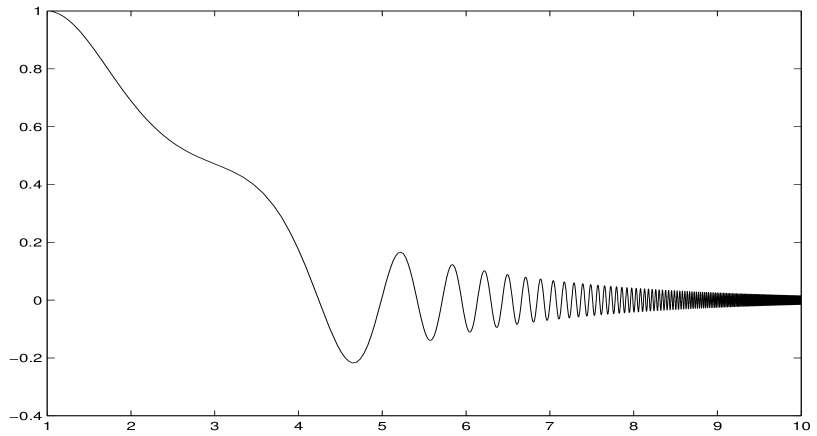
Figure 2.1: Evolution of the expectation value $\eta$ according to eq. (2.32) and (2.33). Here $s=-1$ and $g=1$

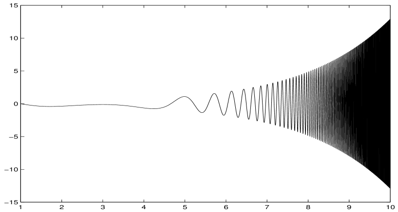
Figure 2.2: Evolution of the expectation value speed $\eta^{\prime}$ according to eq. (2.32) and (2.33), for the values of the parameters as in fig 2.1

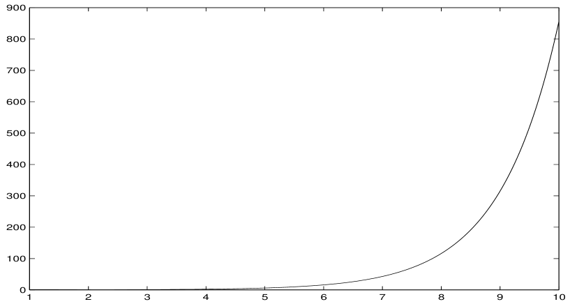
Figure 2.3: Evolution of the quantum width $a$, according to eq. (2.32) and (2.33)

This anomalous behavior is due to the fact that the energy of the fluctuations (2.38) is not bounded from below if $s=-1$. It introduces an inconsistency in our computation scheme: the evolution equations (2.9), (2.10) or equally (2.32) and (2.33) have been obtained supposing the quantum fluctuations were small (in some sense) with respect to the “classical” variable. Instead, the result I get here shows that the fluctuations grow up exponentially for $t\rightarrow\infty$.

Clearly, this behavior is the proof that a complete dynamical treatment is only possible in the framework of a non perturbative approximation scheme, which contains a (at least) partial resummation of the perturbative series.

Hartree-Fock

A first resummation scheme which may be implemented is the time–dependent Hartree-Fock (HF) approximation, which goes as follows. One considers the following substitutions:

$$\xi^{2n} \to \dfrac{(2n)!}{2^{n}(n-1)!}\langle\xi^{2}\rangle^{n-1}\,\xi^{2}-\dfrac{(2n)!(n-1)}{2^{n}n!}\langle\xi^{2}\rangle^{n}\;,$$

$$\xi^{2n+1} \to \dfrac{(2n+1)!}{2^{n}n!}\langle\xi^{2}\rangle^{n}\xi\;.$$ (2.39)

The coefficients of the terms in the rhs have been fixed by the requirement that the mean values of $\xi^{n}$ is the same both in the free theory and in the quadratic theory obtained by the substitution (2.39) (cfr. [62, 72]).

Given this factorization, any potential $V(q)$ becomes

$$V(x+\sqrt{\hbar}\xi)=\sum_{n=0}^{\infty}\dfrac{\hbar^{n}}{n!}\left(\dfrac{\langle\xi^{2}\rangle}{2}\right)^{n}\left\{V^{(2n)}(x)+\sqrt{\hbar}\xi V^{(2n+1)}(x)+\dfrac{\hbar}{2}\left[\xi^{2}-\langle\xi^{2}\rangle\right]V^{(2n+2)}(x)\right\},$$ (2.40)

where we use the notation

$$V^{(n)}(q)\equiv\dfrac{\delta^{n}}{\delta q^{n}}V(q)\;.$$ (2.41)

In the simple case I am considering here [eq. (2.26)], the equations reduce to

$$\begin{array}[]{ll}\stackrel{{\scriptstyle\cdot\cdot}}{{x}}\;=&-\dfrac{1}{m}V^{\prime}\left(x\right)-\dfrac{\hbar}{m}{\textstyle{V^{\prime\prime\prime}\left(x\right)\over 2}}\left\langle\xi^{2}\right\rangle_{\Psi}\\ \stackrel{{\scriptstyle\cdot\cdot}}{{\xi}}\;=&-\dfrac{1}{m}\left[V^{\prime\prime}\left(x\right)+\hbar\dfrac{V^{(IV)}\left(x\right)}{2}\left\langle\xi^{2}\right\rangle_{\Psi}\right]\xi\end{array}$$ (2.42)

The energy becomes

$$E\left(t\right)=E_{cl}^{(0)}\left(t\right)+\hbar E_{fl}^{(1)}\left(t\right)+\hbar^{2}E_{fl}^{(2)}\left(t\right)$$ (2.43)

where (omitting the _Ψ symbol to the mean value)

$$\begin{array}[]{ll}E_{cl}^{(0)}\left(t\right)\;=&\dfrac{m}{2}\dot{x}^{2}+V\left(x\right)\\ E_{fl}^{(1)}\left(t\right)\;=&\dfrac{m}{2}\left\langle\dot{\xi}^{2}\right\rangle+{\textstyle{V^{\prime\prime}\left(x\right)\over 2}}\left\langle\xi^{2}\right\rangle\\ E_{fl}^{(2)}\left(t\right)\;=&\dfrac{V^{(IV)}\left(x\right)}{8}\left\langle\xi^{2}\right\rangle^{2}\end{array}$$ (2.44)

Even if the evolution equation obtained for the operator $\xi\left(t\right)$ contains a cubic term ($\simeq\xi^{3}$), still it can be solved, writing its general solution as a linear combination (with operatorial coefficients) of two real functions, in a way completely similar to that used in the section 2.4.1; it is also labor-saving to use the $\sigma$ variable defined in (2.27); the equations of motion are:

$$\begin{split}\ddot{x}&=-\dfrac{1}{m}V^{\prime}\left(x\right)-\dfrac{\hbar}{m}\dfrac{V^{\prime\prime\prime}\left(x\right)}{2}\sigma^{2}\\ \ddot{\sigma}&=-\dfrac{1}{m}\left[V^{\prime\prime}\left(x\right)+\hbar\dfrac{V^{(IV)}\left(x\right)}{2}\sigma^{2}\right]\sigma+\dfrac{1}{4m^{2}\sigma^{3}}\end{split}$$ (2.45)

with the initial conditions

$$x\left(0\right)=\bar{x}\quad\dot{x}\left(0\right)=0\quad\sigma\left(0\right)=\dfrac{\sigma_{0}}{\sqrt{\hbar}}\quad\dot{\sigma}\left(0\right)=0$$ (2.46)

These equations of motion can be derived by a Lagrangian/Hamiltonian principle, starting with a Lagrangian

$$L\left(x,\dot{x};\sigma,\dot{\sigma}\right)=\dfrac{m}{2}\dot{x}^{2}+\dfrac{m\hbar}{2}\dot{\sigma}^{2}-V\left(x\right)-\dfrac{m\hbar}{2}\dfrac{1}{4m^{2}\sigma^{2}}-\dfrac{\hbar}{2}V^{\prime\prime}\left(x\right)\sigma^{2}-\dfrac{\hbar}{8}V^{(IV)}\left(x\right)\sigma^{4}$$ (2.47)

By means of a Legendre transformation I get the Hamiltonian function, that is the energy (2.43), expressed in terms of the canonical variables $\left\{x(t),\sigma(t)\right\}$ and their conjugated momenta. Deriving the Hamilton equations for this Hamiltonian yields exactly the evolution equations (2.45). A more general view on this subject can be found in the framework of the dissipation and decoherence in field theory, as explained in [55].

I come back to the specific case considered in the previous section. By defining dimensionless dynamical variables as in (2.30) and (2.31) I get the following evolution equations

$$\begin{split}&\eta^{\prime\prime}+s\eta+\eta^{3}+ga^{2}\eta=0\\ &a^{\prime\prime}+sa+3\eta^{2}a-\dfrac{1}{16a^{3}}+ga^{3}=0\end{split}$$ (2.48)

with the initial conditions

$$\eta\left(0\right)=\sqrt{\dfrac{\lambda}{6m\omega^{2}}}\bar{x}=\alpha a\left(0\right)=\sigma_{0}\sqrt{\dfrac{m\omega}{2\hbar}}=\beta$$ (2.49)

$$\eta^{\prime}\left(0\right)=0 a^{\prime}\left(0\right)=0$$ (2.50)

and the following expression for the energy

$$\varepsilon=\eta^{\prime 2}+s\eta^{2}+\dfrac{\eta^{4}}{2}+$$

$$+\dfrac{g}{3}\left[a^{\prime 2}+\left(s+3\eta^{2}\right)a^{2}+\dfrac{g}{2}a^{4}+\dfrac{1}{16a^{2}}\right]$$ (2.51)

From the last expression above we can explicitly see that the energy is now bounded from below and the fluctuations cannot grow up indefinitely for any value of $\eta$.

Variational Principle

It is well known that the quantum evolution in time is given by minimizing the following functional

$$\delta\int dt\,\langle i\partial_{t}-H\rangle=0\;,\quad\langle\cdot\rangle\equiv\left\langle\Psi(t)\right|\cdot\left|\Psi(t)\right\rangle$$ (2.52)

with respect to variations of the wavefunction $\Psi(t)$. Now, let us restrict the Hilbert space to gaussian wavefunctions

$$\Psi(x|\alpha(t),\beta(t))=\left(\dfrac{2{\rm Re\,}\beta}{\pi}\right)^{1/4}\exp\left(-\dfrac{({\rm Re\,}\alpha)^{2}}{4{\rm Re\,}\beta}\right)\exp\left(\alpha x+\beta x^{2}\right)$$

with $\alpha$ and $\beta$ complex parameters, related to mean values and widths of the position and momentum operators. The expectation value in eq. (2.52) becomes a function of the parameters specifying the waefunction and of their first derivatives

$$\int dt\,\langle i\partial_{t}-H\rangle=\int dt\,\Lambda(\alpha(t),\beta(t),\dot{\alpha}(t),\dot{\beta}(t))=\Sigma$$

The stationary condition on the “action” $\Sigma$, $\delta\Sigma=0$, yields a set of Euler–Lagrangian equations for the “Lagrangian” $\Lambda$, which are first order in $\alpha$ and $\beta$ but are completely equivalent to (2.45) or (2.48). This argument shows how the Hartree–Fock approach is based on a gaussian ansatz for the wavefunction.

Large $N$

As we have just seen the HF approximation considers a gaussian state, which evolves in a self-consistently determined quadratic potential, as is obtained from the original theory by means of the HF factorization. The potential felt by the gaussian state and the consequent evolution are self–consistent, in the sense that they depend upon the same parameters which specifies the wave function.

I introduce in this section a different non perturbative approximation scheme, that nevertheless shares similar features with HF. I generalize our system considering a set of $N$ harmonic oscillators described by the canonical coordinates ${q_{1},...,q_{N}}$ and interacting by the $O(N)$ symmetric potential

$$V\left(q_{1},...,q_{N}\right)=\dfrac{1}{2}sm\omega^{2}q\cdot q+\dfrac{\lambda}{4!}\left(q\cdot q\right)^{2}$$ (2.53)

It is well known that the limit $N\to\infty$ yields a well-defined theory provided I rescale the coupling constant in such a way that $\lambda\,N\sim\,\,$constant. As is shown in [73], the theory resulting from the large $N$ limit at leading order can be fully described by means of a set of generalized coherent states. In other words, for $N$ large, only Gaussian states are relevant for the description of the system. Thus, the same factorization as in HF can be performed in this limit, with the difference that here it is exact (at $N=\infty$), while previously was only an approximation, basically out of control.

I now want to get dynamical equations for this system when $N\to\infty$. To this end, I split the position operator of each oscillator in this way:

$$q_{i}=\sqrt{N}x_{i}+\sqrt{\hbar}\xi_{i}$$ (2.54)

The Heisenberg evolution equations turn out to be:

$$\left(\dfrac{d^{2}}{dt^{2}}+s\omega^{2}\right)q_{i}=-\dfrac{1}{N}\dfrac{1}{3!}\dfrac{\Lambda}{m}q^{2}q_{i}$$ (2.55)

where $q^{2}=\sum_{j=1}^{N}q_{j}^{2}$, $i$ going from $1$ to $N$ and $\Lambda=\lambda N$ (not to be confused with the ultraviolet cutoff of QFT, which I will introduce later). Again, I adopt an Hartree-Fock approximation:

$$\xi_{i}\xi_{j}=\langle\xi_{i}\xi_{j}\rangle$$ (2.56)

$$\xi^{2}\xi_{j}=\langle\xi^{2}\rangle\xi_{j}+2\langle\xi_{i}\xi_{j}\rangle\xi_{i}$$ (2.57)

and I obtain the following evolution equations

$$\left(\dfrac{d^{2}}{dt^{2}}+s\omega^{2}\right)x_{i}=-\dfrac{1}{3!}\dfrac{\Lambda}{m}\left(x^{2}x_{i}+\dfrac{2\hbar}{N}x_{j}\langle\xi_{i}\xi_{j}\rangle+\dfrac{\hbar}{N}x_{i}\langle\xi^{2}\rangle\right)$$ (2.58)

$$\left(\dfrac{d^{2}}{dt^{2}}+s\omega^{2}\right)\xi_{j}=-\dfrac{1}{3!}\dfrac{\Lambda}{m}\left[x^{2}\xi_{j}+2x\cdot\xi x_{j}+\dfrac{\hbar}{N}\left(\langle\xi^{2}\rangle\xi x_{j}+2\langle\xi_{i}\xi_{j}\rangle\right)\xi x_{i}\right]$$ (2.59)

Now, when $N=\infty$ I can consistently assume that $x=\left(0,\cdots,u\right)$. Neglecting terms $O(1/N)$, the equations have a solution of the kind $x_{i}\left(t\right)=0$ for $i=1\cdots N-1$. I split the degrees of freedom in transverse ($i=1\cdots N-1$) and longitudinal ($i=N$) and I get the equations:

$$\left(\dfrac{d^{2}}{dt^{2}}+s\omega^{2}\right)u=-\dfrac{1}{3!}\dfrac{\Lambda}{m}\left(u^{3}+\dfrac{\hbar}{N}\langle\xi_{\perp}^{2}\rangle u\right)$$ (2.60)

$$\left(\dfrac{d^{2}}{dt^{2}}+s\omega^{2}\right)\xi_{j}=-\dfrac{1}{3!}\dfrac{\Lambda}{m}u^{2}\xi_{j}$$ (2.61)

$$\left(\dfrac{d^{2}}{dt^{2}}+s\omega^{2}\right)\xi_{N}=-\dfrac{\Lambda}{2m}u^{2}\xi_{N}$$ (2.62)

with the obvious definition $\xi_{\perp}^{2}=\sum_{i=1}^{N-1}\xi_{i}^{2}$. In the large $N$ limit, the difference between ${\textstyle{1\over N}}\xi^{2}$ and ${\textstyle{1\over N}}\xi^{2}_{\perp}$ is $O(1/N)$, thus negligible.

The first two equations (the second equation refers to the transverse fluctuations only) do not depend in any way upon the longitudinal fluctuation $\xi_{N}$ and so they form a ‘closed system’. I can take advantage of the $O\left(N-1\right)$ residual symmetry to write:

$$\langle\xi_{i}\xi_{j}\rangle=\langle\xi_{1}^{2}\rangle\delta_{ij}$$ (2.63)

$$\langle\xi_{i}\xi_{N}\rangle=\langle\xi_{1}\xi_{N}\rangle$$ (2.64)

Of course, in order to these identities be valid, the initial state needs to have the same symmetry as the dynamics which I take the equation from. I get the following evolution equations to leading order in the $1/N$ expansion:

$$\left(\dfrac{d^{2}}{dt^{2}}+s\omega^{2}\right)u=-\dfrac{1}{3!}\dfrac{\Lambda}{m}\left(u^{3}+\hbar\langle\xi_{1}^{2}\rangle u\right)$$ (2.65)

$$\left(\dfrac{d^{2}}{dt^{2}}+s\omega^{2}\right)\xi_{1}=-\dfrac{1}{3!}\dfrac{\Lambda}{m}\left(u^{2}+\hbar\langle\xi_{1}^{2}\rangle\right)\xi_{1}$$ (2.66)

together with the equation for the longitudinal fluctuation (which will be neglected):

$$\left(\dfrac{d^{2}}{dt^{2}}+\omega^{2}\right)\xi_{N}=-\dfrac{1}{3!}\dfrac{\Lambda}{m}\left[\left(3u^{2}+\hbar\langle\xi_{1}^{2}\rangle\right)\xi_{N}+2\hbar\langle\xi_{1}\xi_{N}\rangle\sum_{i=1}^{N-1}\xi_{i}\right]$$ (2.67)

I use similar definitions to (2.27), (2.28) and the dimensionless variables already considered previously [cfr. (2.30) and (2.31)], obtaining the equations:

$$\begin{split}\eta^{\prime\prime}+s\eta+\eta^{3}+\dfrac{g}{3}a^{2}\eta=0\\ a^{\prime\prime}+sa+\eta^{2}a-\dfrac{1}{16a^{3}}+\dfrac{g}{3}a^{3}=0\end{split}$$ (2.68)

with the initial conditions

$$\eta\left(0\right)=\sqrt{\dfrac{\lambda}{6m\omega^{2}}}\bar{x}=\alpha a\left(0\right)=\sigma_{0}\sqrt{\dfrac{m\omega}{2\hbar}}=\beta$$ (2.69)

$$\eta^{\prime}\left(0\right)=0 a^{\prime}\left(0\right)=0$$ (2.70)

The expression of the energy per oscillator in dimensionful variables is the following

$$\dfrac{E}{N}=\dfrac{m}{2}\left(\dot{u}^{2}+\hbar\left\langle\dot{\xi}_{1}^{2}\right\rangle\right)+\dfrac{sm\omega^{2}}{2}\left(u^{2}+\hbar\langle\xi_{1}^{2}\rangle\right)+\dfrac{\Lambda}{4!}\left(u^{2}+\hbar\langle\xi_{1}^{2}\rangle\right)^{2}$$ (2.71)

while I have, in dimensionless variables

$$\varepsilon=\eta^{\prime 2}+s\eta^{2}+\dfrac{\eta^{4}}{2}+$$

$$+\dfrac{g}{3}\left[a^{\prime 2}+\left(s+\eta^{2}\right)a^{2}+\dfrac{g}{6}a^{4}+\dfrac{1}{16a^{2}}\right]$$ (2.72)

which could have been obtained from eqs. (2.3) and (2.26) by means of the substitution $q^{2}\to u^{2}+\hbar\langle\xi_{1}^{2}\rangle$ and $p^{2}\to m^{2}\,\left(\dot{u}^{2}+\hbar\langle\dot{\xi}_{1}^{2}\rangle\right)$. It is interesting to notice the factor of $3$ of difference between this case and the HF approximation considered before, which is due to the different coupling of the longitudinal mode with respect to the transverse ones. This will have important consequences on the renormalizability of the field theoretical model considered in the following sections.

The main advantage of the large $N$ limit is the possibility of obtaining a closed system of equations, considering just the $1-$point and $2-$point functions, thanks to its Gaussian nature. On the other hand, it is generally believed that in this way the contribution of scattering processes is neglected; thus, the resulting theory has infinitely many conserved quantities, which prevent thermalization. Considering $O(1/N)$ corrections is supposed to give an answer to the fundamental question of whether the inclusion of scattering leads to thermalization. Of course, in this case the equations become very difficult to study. In fact, the evolution of each single $n-$point function needs be considered in the treatment, because the exact system is not closed anymore. This makes the problem impossible to be treated numerically and, for any practical purpose, some approximation must be inserted by hand. Bettencourt and Wetterich, for example, consider also the $4-$point function, but neglect all contributions from 1PI $6-$point vertices [74]. As a result, this truncation method converges for large $N$ and is well suited to describe an approach to thermal equilibrium; but, isolated systems do not thermalize even in this further approximation.

Conclusions

I close this section with some comments on the results obtained. We have analyzed interaction phenomena between classical degrees of freedom (mean values) and quantum fluctuations, that produce energy transfer behavior. Yet, we can not speak about a real dissipation of the classical energy, or an irreversible flux of energy towards the quantum degrees of freedom. In fact, to a phase in which the energy flows from one side to the other, it follows immediately an other one, in which the opposite process takes place. The scenario will be completely different in the case of the Quantum Field Theory, where the momentum modes will play the role of infinitely many dissipative channels, producing an effectively irreversible transfer of energy from the classical to the quantum part.

For completeness’ sake, it should be noticed that the $N-$dimensional anisotropic harmonic oscillator in the radial quartic potential is completely integrable, as it has $N$ integrals of motion, which can be naturally constructed by means of a Lax type representation [75]. The same procedure has been used in QFT, to get an infinite hierarchy of sum rules [76].

2.5 Cutoff field theory

After this brief excursus in quantum mechanics, let us come to the main subject of this thesis, the dynamical evolution in quantum field theory. I start introducing the basic vocabulary and instruments I will be using in the following: I consider the $N-$component scalar field operator $\boldsymbol{\phi}$ in a $D-$dimensional periodic box of size $L$ and write its Fourier expansion as customary

$$\boldsymbol{\phi}(x)=L^{-D/2}\sum_{k}\boldsymbol{\phi}_{k}\,e^{ik\cdot x}\;,\quad\boldsymbol{\phi}_{k}^{\dagger}=\boldsymbol{\phi}_{-k}$$ (2.73)

with the wavevectors $k$ naturally quantized: $k=(2\pi/L)n$, $n\in{\cal Z}^{D}$. The canonically conjugated momentum $\boldsymbol{\pi}$ has a similar expansion

$$\boldsymbol{\pi}(x)=L^{-D/2}\sum_{k}\boldsymbol{\pi}_{k}\,e^{ik\cdot x}\;,\quad\boldsymbol{\pi}_{k}^{\dagger}=\boldsymbol{\pi}_{-k}$$ (2.74)

with the commutation rules $[\phi_{k}^{\alpha}\,,\pi_{-k^{\prime}}^{\beta}]=i\,\delta^{(D)}_{kk^{\prime}}\,\delta^{\alpha\beta}$. Of course, when the size $L$ goes to $\infty$, the sums become integrals over a continuum of momentum modes.

To regularize the ultraviolet behavior, I restrict the sums over wavevectors to the points lying within the $D-$dimensional sphere of radius $\Lambda$, that is $k^{2}\leq\Lambda^{2}$, with ${\cal N}=\Lambda L/2\pi$ some large integer. Clearly, as long as both the cutoffs remain finite, I have reduced the original field–theoretical problem to a quantum–mechanical framework with finitely many (of order ${\cal N}^{D-1}$) degrees of freedom.

The $\phi^{4}$ Hamiltonian reads

$$H = \dfrac{1}{2}\int d^{D}x\left[\boldsymbol{\pi}^{2}+(\partial\boldsymbol{\phi})^{2}+m^{2}_{\rm b}\,\boldsymbol{\phi}^{2}+\dfrac{\lambda_{\rm b}}{2}(\boldsymbol{\phi}^{2})^{2}\right]$$ (2.75)

$$= \dfrac{1}{2}\sum_{k}\left[\boldsymbol{\pi}_{k}\!\cdot\boldsymbol{\pi}_{-k}+(k^{2}+m^{2}_{\rm b})\,\boldsymbol{\phi}_{k}\!\cdot\boldsymbol{\phi}_{-k}\right]+$$

$$+ \dfrac{\lambda_{\rm b}}{4L^{D}}\sum_{k_{1},k_{2},k_{3},k_{4}}(\boldsymbol{\phi}_{k_{1}}\!\!\cdot\boldsymbol{\phi}_{k_{2}})(\boldsymbol{\phi}_{k_{3}}\!\!\cdot\boldsymbol{\phi}_{k_{4}})\,\delta^{(D)}_{k_{1}+k_{2}+k_{3}+k_{4},0}$$

where $m^{2}_{\rm b}$ and $\lambda_{\rm b}$ should depend on the UV cutoff $\Lambda$ in such a way to guarantee a finite limit $\Lambda\to\infty$ for all observable quantities. As is known [14, 61], this implies triviality (that is vanishing of renormalized vertex functions with more than two external lines) for $D>3$ and very likely also for $D=3$. In the latter case triviality is manifest in the one–loop approximation and in large$-N$ limit due to the Landau pole. For this reason I shall keep $\Lambda$ finite and regard the $\phi^{4}$ model as an effective low–energy theory (here low–energy means practically all energies below Planck’s scale, due to the large value of the Landau pole for renormalized coupling constants of order one or less).

I shall work in the wavefunction representation where $\left\langle\boldsymbol{\varphi}\right|\left.\Psi\right\rangle=\Psi(\boldsymbol{\varphi})$ and

$$(\boldsymbol{\phi}_{0}\Psi)(\boldsymbol{\varphi})=\boldsymbol{\varphi}_{0}\Psi(\boldsymbol{\varphi})\;,\quad(\boldsymbol{\pi}_{0}\Psi)(\boldsymbol{\varphi})=-i\dfrac{\partial}{\partial\boldsymbol{\varphi}_{0}}\Psi(\boldsymbol{\varphi})$$ (2.76)

while for $k>0$ (in lexicographic sense)

$$(\boldsymbol{\phi}_{\pm k}\Psi)(\boldsymbol{\varphi})=\dfrac{1}{\sqrt{2}}\left(\boldsymbol{\varphi}_{k}\pm i\,\boldsymbol{\varphi}_{-k}\right)\Psi(\boldsymbol{\varphi})\;,\quad(\boldsymbol{\pi}_{\pm k}\Psi)(\boldsymbol{\varphi})=\dfrac{1}{\sqrt{2}}\left(-i\dfrac{\partial}{\partial\boldsymbol{\varphi}_{k}}\pm\dfrac{\partial}{\partial\boldsymbol{\varphi}_{-k}}\right)\Psi(\boldsymbol{\varphi})$$ (2.77)

Notice that by construction the variables $\boldsymbol{\varphi}_{k}$ are all real. Of course, when either one of the cutoffs are removed, the wave function $\Psi(\boldsymbol{\varphi})$ acquires infinitely many arguments and becomes what is usually called a wavefunctional.

In practice, the problem of studying the dynamics of the $\phi^{4}$ field theory out of equilibrium consists now in trying to solve the time-dependent Schroedinger equation given an initial wavefunction $\Psi(\boldsymbol{\varphi},t=0)$ that describes a state of the field far away from the vacuum. By this I mean a non–stationary state that, in the infinite volume limit $L\to\infty$, would lay outside the particle Fock space constructed upon the vacuum. This approach could be generalized in a straightforward way to mixtures described by density matrices, as done, for instance, in [42, 53, 62]. Here I shall restrict to pure states, for sake of simplicity and because all relevant aspects of the problem are already present in this case.

A completely equivalent approach to the time dependent problem in QFT is based on the Heisenberg representation, where the operators are time dependent while the states are fixed. In such an approach, the evolution equations for the field condensate and the correlation functions may be obtained by a generalization of the tadpole equation to time dependent situations, starting from the Heisenberg equations for the operators, as already shown in section 2.4.1.

A rigorous result: the effective potential is convex

I want to stress that the introduction of both a UV and IR cutoff allows to easily derive the well–known rigorous result concerning the flatness of the effective potential. In fact $V_{\rm eff}(\bar{\phi})$ is a convex analytic function in a finite neighborhood of $\bar{\phi}=0$, as long as the cutoffs are present, due to the uniqueness of the ground state. This is a well known fact in statistical mechanics, being directly related to stability requirements. It would therefore hold also for the field theory in the Euclidean functional formulation. In our quantum–mechanical context I may proceed as follows. Suppose the field $\phi$ is coupled to a uniform external source $J$. Then the ground state energy $E_{0}(J)$ is a concave function of $J$, as can be inferred from the negativity of the second order term in $\Delta J$ of perturbation around any chosen value of $J$. Moreover, $E_{0}(J)$ is analytic in a finite neighborhood of $J=0$, since $J\phi$ is a perturbation “small” compared to the quadratic and quartic terms of the Hamiltonian. As a consequence, this effective potential $V_{\rm eff}(\bar{\phi})=E_{0}(J)-J\bar{\phi}$, $\bar{\phi}=E_{0}^{\prime}(J)=\langle\phi\rangle_{0}$, that is the Legendre transform of $E_{0}(J)$, is a convex analytic function in a finite neighborhood of $\bar{\phi}=0$. In the infrared limit $L\to\infty$, $E_{0}(J)$ might develop a singularity in $J=0$ and $V_{\rm eff}(\bar{\phi})$ might flatten around $\bar{\phi}=0$. Of course this possibility would apply in case of spontaneous symmetry breaking, that is for a double–well classical potential [77, 78]. This is a subtle and important point that will play a crucial role later on, even if the effective potential is relevant for the static properties of the model rather than the dynamical evolution out of equilibrium that interests us here. In fact such evolution is governed by the CTP effective action [29, 32] and one might expect that, although non–local in time, it asymptotically reduces to a multiple of the effective potential for trajectories of $\bar{\phi}(t)$ with a fixed point at infinite time. In such case there should exist a one–to–one correspondence between fixed points and minima of the effective potential.

2.6 Evolution of a homogeneous background

The dynamics of uniform strongly out of equilibrium condensates in QFT has been studied mainly in connection with the phenomenology of heavy ion collisions and with the evolution of the Early Universe. It has become clear that phenomena associated with parametric amplification of quantum fluctuations can play an important role in the process of reheating and thermalization. It should be emphasized, however, that the dynamics in cosmological backgrounds differs qualitatively and quantitatively from the dynamics in Minkovski space. In any case, in such situations, the quantum state is characterized by a large energy density, which means a large number of particles per correlation volume $m^{-3}$.

The simplest case we can start with is the evolution of a translation invariant state, which has a uniform field mean value. This kind of simplification is fully justified in cosmological scenarios, where the exponential expansion make all disuniformities to disappear, while we need surely something better in order to study the out of equilibirum phenomena occurring during and after a heavy ion collision. We consider here the case of an uniform condensate, postponing the discussion on the evolution of a spherically symmetric state to section 2.11.

2.6.1 Two words on perturbative approaches

As already pointed out in section 2.4.3, there exist several approximation schemes to solve a time dependent problem. Enforcing a double perturbative expansion, both in the number of loops and in the field amplitude, we get the following equation of motion, for a uniform expectation value of a quantum scalar field (to one–loop level and to cubic order in field amplitude) [61]:

$$\ddot{\phi}(t)+m^{2}\phi(t)+\dfrac{\lambda}{6}\phi^{3}(t)+\dfrac{\lambda^{2}}{4}\phi(t)\int_{t_{0}}^{t}dt^{\prime}\phi(t^{\prime})\dot{\phi}(t^{\prime})\int\dfrac{d^{3}k}{(2\pi)^{3}}\dfrac{\cos[2\omega_{k}(t-t^{\prime})]}{2\omega_{k}^{3}}=0$$ (2.78)

where $\lambda$ and $m^{2}$ are the renormalized coupling constant and mass and $\omega_{k}=\sqrt{k^{2}+m^{2}}$. de Vega and Salgado [79] solved analytically this non linear and non local equation by RG techniques. The exact solution shows that the order parameter oscillates as the classical cnoidal solution with slowly time dependent amplitude and frequency. In addition, the amplitude reaches an asymptotic value, which is a function of the initial amplitude, as $t^{-3/2}$.

I can also solve the one loop equations exactly in the field amplitude. In this case, I reach the conclusion [61] that perturbation theory is not suitable for the purpose of studying the asymptotic dynamics of a quantum system. Due to parametric resonances and/or spinodal instabilities there are modes of the field that grow exponentially in time until they produce non–perturbative effects for any coupling constant, no matter how small. For this reason, the perturbative approach can be considered valid only for the early time evolution. On the other hand, only few, by now standard, approximate non–perturbative schemes are available for the $\phi^{4}$ theory, and to these I have to resort after all. I shall consider the large $N$ expansion to leading order in section 2.7 (cfr. ref. [80]), remanding to the definition of a time-dependent Hartree–Fock (tdHF) approach (a generalization of the treatment given, for instance, in [18]) to section 2.10 (cfr. ref. [81]). In fact these two methods are very closely related, as shown in [69], where several techniques to derive reasonable dynamical evolution equations for non–equilibrium $\phi^{4}$ are compared.

2.7 Large $N$ expansion at leading order

2.7.1 Definitions

In this section I consider a standard non–perturbative approach to the $\phi^{4}$ model which is applicable also out of equilibrium, namely the large $N$ method as presented in [55]. However I shall follow a different derivation which makes the gaussian nature of the $N\to\infty$ limit more explicit.

It is known that the theory described by the Hamiltonian (2.75) is well behaved for large $N$, provided that the quartic coupling constant $\lambda_{\rm b}$ is rescaled with $1/N$. For example, it is possible to define a perturbation theory, based on the small expansion parameter $1/N$, in the framework of which one can compute any quantity at any chosen order in $1/N$. From the diagrammatic point of view, this procedure corresponds to a resummation of the usual perturbative series that automatically collects all the graphs of a given order in $1/N$ together [20]. Moreover, it has been established since the early 80’s that the leading order approximation (that is the strict limit $N\to\infty$) is actually a classical limit [73], in the sense that there exists a classical system (i.e., a classical phase space, a Poisson bracket and a classical Hamiltonian) whose dynamics controls the evolution of all fundamental quantum observables, such as field correlation functions, in the $N\to\infty$ limit. For instance, from the absolute minimum of the classical Hamiltonian one reads the energy of the ground state, while the spectrum is given by the frequencies of small oscillations about this minimum, etc. etc.. I am here interested in finding an efficient and rapid way to compute the quantum evolution equations for some observables in the $N\to\infty$ limit, and we will see that this task is easily accomplished just by deriving the canonical Hamilton equations from the large $N$ classical Hamiltonian.

Following Yaffe [73], I write the quantum mechanical hamiltonian as

$$H=Nh(A\,,C)$$ (2.79)

in terms of the square matrices $A$, $C$ with operator entries ($\boldsymbol{\varpi}_{k}$ is the canonical momentum conjugated to the real mode $\boldsymbol{\varphi}_{k}$)

$$A_{kk^{\prime}}=\dfrac{1}{N}\boldsymbol{\varphi}_{k}\!\cdot\boldsymbol{\varphi}_{k^{\prime}}\;,\quad C_{kk^{\prime}}=\dfrac{1}{N}\boldsymbol{\varpi}_{k}\!\cdot\boldsymbol{\varpi}_{k^{\prime}}$$ (2.80)

These are example of “classical” operators, whose two-point correlation functions factorize in the $N\to\infty$ limit. This can be shown by considering the coherent states

$$\Psi_{z,q,p}(\boldsymbol{\varphi})=C(z)\exp\left[i\sqrt{N}\sum_{k}\boldsymbol{p}_{k}\cdot\boldsymbol{\varphi}_{k}-\dfrac{1}{2}\sum_{kk^{\prime}}z_{kk^{\prime}}(\boldsymbol{\varphi}_{k}-\sqrt{N}\boldsymbol{q}_{k})\cdot(\boldsymbol{\varphi}_{k^{\prime}}-\sqrt{N}\boldsymbol{q}_{k^{\prime}})\right]$$ (2.81)

where the complex symmetric matrix $z$ has a positive definite real part while $\boldsymbol{p}_{k}$ and $\boldsymbol{q}_{k}$ are real and coincide, respectively, with the coherent state expectation values of $\boldsymbol{\varpi}_{k}$ and $\boldsymbol{\varphi}_{k}$. As these parameters take all their possible values, the coherent states form an overcomplete set in the cutoff Hilbert space of the model. The crucial property which ensures factorization is that they become all orthogonal in the $N\to\infty$ limit. Moreover one can show [73] that the coherent states parameters form a classical phase space with Poisson brackets

$$\left\{q_{k}^{i}\,,p_{k^{\prime}}^{j}\right\}_{\rm P.B.}=\delta_{kk^{\prime}}\delta^{ij}\;,\quad\left\{w_{kk^{\prime}}\,,v_{qq^{\prime}}\right\}_{\rm P.B.}=\delta_{kq}\delta_{k^{\prime}q^{\prime}}+\delta_{kq^{\prime}}\delta_{k^{\prime}q}$$ (2.82)

where $w$ and $v$ reparametrize $z$ as $z={\textstyle{1\over 2}}w^{-1}+i\,v$. It is understood that the dimensionality of the vectors $\boldsymbol{q}_{k}$ and $\boldsymbol{p}_{k}$ is arbitrary but finite [that is, only a finite number, say $n$, of pairs $(\varphi_{k}^{i}\,,\varpi_{k}^{i})$ may take a non vanishing expectation value as $N\to\infty$].

Once applied to the classical operators $A_{kk^{\prime}}$ and $C_{kk^{\prime}}$ the large $N$ factorization allows to obtain the classical hamiltonian by simply replacing $A$ and $C$ in eq. (2.79) by the coherent expectation values

$$\langle A_{kk^{\prime}}\rangle=\boldsymbol{q}_{k}\cdot\boldsymbol{q}_{k^{\prime}}+w_{kk^{\prime}}\;,\quad\langle C_{kk^{\prime}}\rangle=\boldsymbol{p}_{k}\cdot\boldsymbol{p}_{k^{\prime}}+(v\,w\,v)_{kk^{\prime}}+\dfrac{1}{4}(w^{-1})_{kk^{\prime}}$$ (2.83)

In the situation considered, having assumed a uniform background expectation value for $\boldsymbol{\phi}$, I have $\boldsymbol{q}_{k}=\boldsymbol{p}_{k}=0$ for all $k\neq 0$; moreover, translation invariance implies that $w$ and $v$ are diagonal matrices, so that I may set

$$w_{kk^{\prime}}=\sigma_{k}^{2}\,\delta_{kk^{\prime}}\;,\quad v_{kk^{\prime}}=\dfrac{s_{k}}{\sigma_{k}}\,\delta_{kk^{\prime}}$$ (2.84)

in term of the canonical couples $(\sigma_{k},s_{k})$ which satisfy $\{\sigma_{k}\,,s_{k^{\prime}}\}_{\rm P.B.}=\delta_{kk^{\prime}}$. Notice that the $\sigma_{k}$ are just the widths (rescaled by $N^{-1/2}$) of the $O(N)$ symmetric and translation invariant gaussian coherent states.

Thus I find the classical hamiltonian

$$h_{\rm cl}=\dfrac{1}{2}(\boldsymbol{p}_{0}^{2}+m^{2}_{\rm b}\,\boldsymbol{q}^{2}_{0})+\dfrac{1}{2}\sum_{k}\left[s_{k}^{2}+(k^{2}+m^{2}_{\rm b})\sigma_{k}^{2}+\dfrac{1}{4\sigma^{2}_{k}}\right]+\dfrac{\lambda_{\rm b}}{4L^{D}}\left(\boldsymbol{q}_{0}^{2}+\sum_{k}\sigma_{k}^{2}\right)^{2}$$ (2.85)

where by Hamilton’s equations of motion $\boldsymbol{p}_{0}=\dot{\boldsymbol{q}}_{0}$ and $s_{k}=\dot{\sigma}_{k}$. The corresponding conserved energy density ${\cal E}=L^{-D}h_{\rm cl}$ may be written

$${\cal E} ={\cal T}+{\cal V}\;,\quad{\cal T}=\dfrac{1}{2}\dot{\bar{\boldsymbol{\phi}}}^{2}+\dfrac{1}{2L^{D}}\sum_{k}\dot{\sigma}_{k}^{2}$$ (2.86)

$${\cal V} =\dfrac{1}{2L^{D}}\sum_{k}\left(k^{2}\,\sigma_{k}^{2}+\dfrac{1}{4\sigma^{2}_{k}}\right)+V(\bar{\boldsymbol{\phi}}^{2}+\Sigma)\;,\quad\Sigma=\dfrac{1}{L^{D}}\sum_{k}\sigma_{k}^{2}$$ (2.87)

where $\bar{\boldsymbol{\phi}}=L^{-D/2}\boldsymbol{q}_{0}$ and $V$ is the $O(N)-$invariant quartic potential regarded as a function of $\boldsymbol{\phi}^{2}$, that is $V(z)={\textstyle{1\over 2}}m^{2}_{\rm b}z+{\textstyle{1\over 4}}\lambda_{\rm b}z^{2}$. It is worth noticing that eq. (2.87) would apply as is to generic $V(z)$ and the potential ${\cal V}$, the static part of $h_{\rm cl}$, is what the authors of [55] call the true effective, that is the correct potential for studying the evolution of field configurations far from equilibrium. For state in thermal equilibrium at a temperature $T$, it would correspond to the internal energy $U$. The standard effective potential corresponds, instead, to the free energy $F$. Of course, the information contained in $F$ and in $U$ is very different.

Basically, the evolution equations are Hamilton’s equations for an effective classical Hamiltonian $h_{\rm cl}$ (which contains $\hbar$ as a parameter) given by the the expectation value of the quantum Hamiltonian on the gaussian mixed state described by generalized coherent states. This fact shows that the mean field approximation does not explicitly introduce any dissipative behavior in the system.

In conclusion, in the limit $N\to\infty$, the mean field and the two–point correlation function evolve as a self–consistent closed Hamiltonian system, described by a generalized coherent state (or, more generally, by a guassian density matrix). This corresponds to a truncation of the infinite hierarchy of Schwinger–Dyson equations to $1$ and $2$ point functions.

The connection of the quantum evolution with a classical hamiltonian formalism in mean field approximation has been studied also in [82, 83], generalizing the time–dependent variational principle of Balian and Vénéroni.

As we will see later on (cfr. sec 2.10), the $O(N)$ $\lambda\phi^{4}$ at leading order in $1/N$, is very closely related to the Hartree–Fock mean field approximation which has been much used in nuclear many–body, atomic and molecular chemistry applications.

2.8 Dynamics in Infinite volume

The non equilibrium dynamics of the $O(N)\,\Phi^{4}$ model in the large $N$ limit, in the broken symmetry phase and for state of large energy density has been considered in [84]. The new phenomena discovered by the detailed numerical analysis of the time evolution, are all essentially non perturbative. This character is very well captured by the large $N$ limit, which is also consistently renormalizable and can be systematically improved by considering higher powers in the $1/N$ expansion.

The dynamical analysis in this approximation shows once more that the static effective potential is not suitable to study out of equilibrium evolutions. In fact, it is well known that, at one loop level, it becomes complex in the coexistence region. Since at leading order in $1/N$, the one loop results become exact, the problem cannot be ascribed to the inexactness of the one loop approximation, but in turn suggests that the static effective potential is not able to describe the system when a mixture of phases can occur.

From the dynamical point of view, two different physical situations [84] are possible:

• if the (conserved) energy density $\varepsilon$ is smaller than the local maximum of the tree level potential $V_{0}$ (expressed in terms of the renormalized parameters), then the presence of spinodal instabilities leads to a dynamical Maxwell construction: all the expectation values between the minima are available asymptotically with a vanishing effective mass, dynamically flattening the potential in the coexistence region at $t=\infty$; the dependence of the asymptotic condensate from the initial condition can be well parametrized by the following formula:

  $$\langle\hat{\Phi}(x,t=\infty\rangle=\sqrt{\dfrac{2}{\lambda}}|m|\left[1-\dfrac{\varepsilon}{V_{0}}\right]^{0.25}$$ (2.88)

• if, instead, $\varepsilon>V_{0}$, the evolution is symmetric and the condensate samples ergodically both the minima of the tree level potential, showing that the symmetry is restored at the dynamical level; the mass squared reaches an asymptotic value different from zero while the condensate transfers all of its energy to quantum fluctuations and vanishes asymptotically.

2.8.1 Early time and asymptotic dynamics

The asymptotic dynamics of dissipation and relaxation in scalar field theories, starting from large energy densities, must be studied going beyond the perturbative approach, in an energy conserving and renormalizable framework, able to include self–consistently the effects of quantum back-reaction.

A thorough analytical study and a refined numerical analysis have been provided in [85], where the relaxation of an initial state of large density is observed through the copious production of particles in a collisionless regime, similar to Landau damping in non relativistic electromagnetic plasmas. As a result, the asymptotic distribution is not thermal. In case of spontaneous symmetry breaking, the effects of the massless excitations on the evolution of the mean field may be studied in detail and a linear response analysis shows the presence of a collective plasma mode [55].

The complete evolution can be divided in two parts. The early time evolution is dominated by a so–called “linear regime”, during which the energy initially stored in one (or few) modes of the field is transferred to other modes via either parametric or spinodal instabilities, resulting in a large particle production and a consequent dissipation for the initial condensate [61].

It is worth explaining briefly the mechanism of spinodal decomposition (see also [86]). The effective, coarse-grained description of statistical systems with a spontaneously broken phase, is based on a phenomenological free energy of the Landau-Ginzburg form. This is a quartic functional in the order parameter, with a temperature dependent coefficient for the second order term, which becomes negative when the temperature falls down the critical. Such a functional admits a spinodal region where the potential is non-convex, corresponding to thermodynamically unstable states. When the system approaches the ordered phase, coming from the disordered one, the long wavelength modes become critically slowed down, in the sense that their relaxation time diverges when both the reduced temperature and the momentum go to zero. Thus, they relax to equilibirum on very long time scales. Below the critical temperature, because of the existence of the spinodal region, there is a band of unstable wave vectors, for which the frequencies are positive and the corresponding fluctuations from the mean field grow exponentially. These instabilities are the hallmark of the process of phase separation and are the early time indications of the formation and growth of correlated regions.

The asymptotic evolution at late times is completely non linear and is associated to power law behavior for the growth of quantum fluctuations and the relaxation of the condensate; the power laws contain non–universal and non–perturbative dynamical anomalous exponents. The two regimes are separated by a time scale $t_{\rm s}$, which is non perturbative in the coupling and in the initial amplitude, and is defined as the time when the quantum fluctuations become of the same order as the tree level term in the equations of motion and the dynamics turns completely non linear and non perturbative [61, 85]; the analytical study of the early time evolution [85] shows that $t_{\rm s}\simeq\log 1/\lambda$ (where $\lambda$ is the quartic coupling constant).

The main results may be summarized as follows: (i) thanks to the hierarchy of time scales, a dynamical renormalization group resummation can be applied, showing the existence of non linear resonances which turn the exponential behavior in non–universal power laws with dynamical anomalous exponents; (ii) the effective squared mass felt by the modes is time dependent and tends to an asymptotic value as $O(1/t)$; thus, the quantum modes becomes asymptotically free; (iii) in the unbroken symmetry phase, the condensate relaxes all the way to zero, transferring completely its energy to the quantum fluctuations, in spite of the presence of a perturbative threshold for particle production; (iv) precise sum rules may be established for the asymptotic particle distribution and an equation of state interpolating between the radiation–type and the dust–type is found; (v) in the broken phase, the mass vanishes asymptotically, providing a dynamical realization of the Goldstone theorem; (vi) the asymptotic value of the condensate is a function of the initial amplitude; (vii) at very large time scale, $t\sim\sqrt{V}$ (where $V$ stands for the volume of the system), the non–perturbative and non–linear evolution might eventually produce the onset of a non–equilibrium Bose–Einstein condensation of the long–wavelength Goldstone bosons usually present in the broken symmetry phase of the model [84, 85]; (viii) the asymptotic particle distribution, obtained as the result of the copious particle production at the expenses of the “classical” energy, is strongly non-thermal [61, 85].

Moreover, in this formalism, some aspects of the quantum dynamics of phase ordering can be studied in some detail. The non perturbative spinodal time $t_{s}\simeq\log 1/\lambda$ divides the evolution in two regimes: for $t<t_{s}$ the correlation length $\xi(t)$ grows like $\sqrt{t}$; for $t>t_{s}$, $\xi(t)\simeq 2(t-t_{s})$, the correlation function vanishes for $r>2(t-t_{s})$ and the zero momentum mode of the quantum fluctuations grows asymptotically linearly. Thus, the correlated domains grow at the speed of light and contain inside a non perturbative condensate of Goldstone bosons, with a correlation which decreases as $1/r$.

Another very interesting result in [84] concerns the dynamical Maxwell construction, which reproduces the flat region of the effective potential in case of broken symmetry as asymptotic fixed points of the background evolution.

Finally, using a density matrix language, a semiclassical but stochastic description emerges: after $t_{s}$, semiclassical large amplitude field configurations are represented in $\rho$ with a finite probability.

2.9 Dynamics in Finite volume

In this section I present a detailed study, in finite volume, of dynamical evolution out of equilibrium for the $\Phi^{4}$ scalar field in the large $N$ limit. More precisely, I determine how such dynamics scales with the size of the periodic box containing the system in the case of uniform backgrounds. This is necessary to address questions like out–of–equilibrium symmetry breaking and dynamical Bose–Einstein condensation.

The introduction of a finite volume should be regarded as a regularization of the infrared properties of the model, which allows to “count” the different field modes and is needed especially in the case of broken symmetry. In fact, all the results I have summarized in section 2.8, have been obtained simulating the system directly in infinite volume, where the evolution equations contain momentum integrals, that must be computed numerically by a proper, but nonetheless rather arbitrary, discretization in momentum space. Of course, the final result should be as insensitive as possible to the particular choice of the integration grid. In such a situation, the definition of a “zero” mode and the interpretation of its late time behavior might not be rigorous enough, unless, for some reason, it turns out that a particular mode requires a different treatment compared to the others. In order to understand this point, it is necessary to put the system in a finite volume (a box of size $L$); the periodic boundary conditions let us single out the zero mode in a rigorous way and thus we can carefully analyze its scaling properties with $L$ and get some information on the infinite volume limit. I have defined the model in finite volume, giving all the relevant notations and definitions in section 2.5. I derived the large $N$ approximation of the $O(N)-$invariant version of $\lambda(\boldsymbol{\phi}^{2})^{2}$ model, according to the general rules of ref. [73]. In this derivation it appears evident the essential property of the $N\to\infty$ limit of being a particular type of classical limit, so that it leads to a classical phase space, a classical hamiltonian with associated Hamilton’s equations of motion [see eqs. (2.109), (2.110) and (2.111)].

I then minimize the hamiltonian function(al) and determine the conditions for massless Goldstone bosons (i.e. transverse fluctuations of the field) to form a Bose–Einstein condensate, delocalizing the vacuum field expectation value (cfr. also ref. [55]). This necessarily requires that the width of the zero–mode fluctuations becomes macroscopically large, that is of the order of the volume. Only when the background takes one of the extremal values proper of symmetry breaking the width of the zero–mode fluctuations is of order $L^{1/2}$, as typical of a free massless spectrum.

The study of the lowest energy states of the model is needed for comparison with the results of the numerical simulations, which show that the zero–mode width $\sigma_{0}$ stays microscopic (that is such that $\sigma_{0}/$volume$\to 0$ when the volume diverges) whenever it starts from initial conditions in which it is microscopic. The results, in fact, show clearly the presence of a time scale $\tau_{L}$, proportional to the linear size $L$ of the system, at which finite volume effects start to manifest. I shall give a very simple physical interpretation of this time scale in section 2.9.3. The important point is that after $\tau_{L}$ the zero mode amplitude starts decreasing, then enters an erratic evolution, but never grows macroscopically large. This result is at odd with the interpretation of the linear late–time growth of the zero–mode width as a full dynamical Bose–Einstein condensation of Goldstone bosons, but is compatible with the “novel” form of BEC reported in [65, 84, 85]. In fact I do find that the size of the low–lying widths at time $\tau_{L}$ is of order $L$, to be compared to the equilibrium situation where they would be of order $L^{0}$ in the massive case or of order $L^{1/2}$ in the massless case. Perhaps the denomination “microscopic” should be reserved to this two possibilities. Therefore, since the initial condition are indeed microscopic in this restricted sense, I do observe in the out–of–equilibrium evolution a rapid transition to a different regime intermediate between the microscopic one and the macroscopic one characteristic of Bose–Einstein condensation. As I shall discuss more in detail later on, this fully agrees with the result found in [84], that the time–dependent field correlations vanish at large separations more slowly than for equilibrium free massless fields (as $r^{-1}$ rather than $r^{-2}$), but definitely faster than the equilibrium broken symmetry phase characterized by constant correlations at large distances. At any rate, when one considers microscopic initial conditions for the choice of bare mass which corresponds to broken symmetry, the role itself of symmetry breaking is not very clear in the large $N$ description of the out–of–equilibrium dynamics, making equally obscure the issues concerning the so–called quantum phase ordering [84]. This is because the limit $N\to\infty$ is completely saturated by gaussian states, which might signal the onset of symmetry breaking only developing macroscopically large fluctuations. Since such fluctuations do not appear to be there, the meaning itself of symmetry breaking, as something happening as times goes on and accompanied by some kind of phase ordering, is quite unclear. I postpone to section 2.10 (cfr. also [81]) the discussion about the possibility of using more comprehensive approximation schemes, that include some non–gaussian features of the complete theory. As far as the large $N$ approximation is concerned, I underline that an important limitation of our approach, as well as of those of the references mentioned above, is in any case the assumption of a uniform background. Nonetheless, phenomena like the asymptotic vanishing of the effective mass and the dynamical Maxwell construction, taking place in this contest of a uniform background and large $N$ expansion, are certainly very significant manifestations of symmetry breaking and in particular of the Goldstone theorem which applies when a continuous symmetry is broken.

2.9.1 Static properties

Let us consider first the static aspects embodied in the effective potential $V_{\rm eff}(\bar{\boldsymbol{\phi}})$, that is the minimum of the potential energy ${\cal V}$ at fixed $\bar{\boldsymbol{\phi}}$. I first define in a precise way the unbroken symmetry phase, in this large $N$ context, as the case when $V_{\rm eff}(\bar{\boldsymbol{\phi}})$ has a unique minimum at $\bar{\boldsymbol{\phi}}=0$ in the limit of infinite volume. Minimizing ${\cal V}$ w.r.t. $\sigma_{k}$ yields

$$\sigma^{2}_{k}=\dfrac{1}{2\sqrt{k^{2}+M^{2}}}\;,\quad M^{2}=m^{2}_{\rm b}+2\,V^{\prime}(\bar{\boldsymbol{\phi}}^{2}+\Sigma)$$

$$=m^{2}_{\rm b}+\lambda_{\rm b}\bar{\boldsymbol{\phi}}^{2}+\dfrac{\lambda_{\rm b}}{L^{D}}\sum_{k}\dfrac{1}{2\sqrt{k^{2}+M^{2}}}$$

that is the widths characteristic of a free theory with self–consistent mass $M$ fixed by the gap equation. By the assumption of unbroken symmetry, when $\bar{\boldsymbol{\phi}}=0$ and at infinite volume $M$ coincides with the equilibrium mass $m$ of the theory, that may be regarded as an independent scale parameter. Since in the limit $L\to\infty$ sums are replaced by integrals

$$\Sigma\to\int_{k^{2}\leq\Lambda^{2}}\dfrac{d^{D}k}{(2\pi)^{D}}\sigma_{k}^{2}$$ (2.90)

I obtain the standard bare mass parameterization

$$m^{2}_{\rm b}=m^{2}-\lambda_{\rm b}I_{D}(m^{2},\Lambda)\;,\quad I_{D}(z,\Lambda)\equiv\int_{k^{2}\leq\Lambda^{2}}\dfrac{d^{D}k}{(2\pi)^{D}}\dfrac{1}{2\sqrt{k^{2}+z}}$$ (2.91)

and the renormalized gap equation

$$M^{2}=m^{2}+\lambda\,\bar{\phi}^{2}+\lambda\left[I_{D}(M^{2},\Lambda)-I_{D}(m^{2},\Lambda)\right]_{\rm finite}$$ (2.92)

which implies, when $D=3$,

$$\lambda_{\rm b}=\lambda\left(1-\dfrac{\lambda}{8\pi^{2}}\log\dfrac{2\Lambda}{m\sqrt{e}}\right)^{\!\!-1}$$ (2.93)

with a suitable choice of the finite part. No coupling constant renormalization occurs instead when $D=1$. The renormalized gap equation (2.92) may also be written quite concisely

$$\dfrac{M^{2}}{\hat{\lambda}(M)}=\dfrac{m^{2}}{\hat{\lambda}(m)}+\,\bar{\boldsymbol{\phi}}^{2}$$ (2.94)

in terms of the one–loop running couplings constant

$$\hat{\lambda}(\mu)=\lambda\left[1-\dfrac{\lambda}{8\pi^{2}}\log\dfrac{\mu}{m}\right]^{-1}\;,\quad\hat{\lambda}(m)=\lambda\;,\quad\hat{\lambda}(2\Lambda\,e^{-1/2})=\lambda_{\rm b}$$ (2.95)

It is the Landau pole in $\hat{\lambda}(2\Lambda\,e^{-1/2})$ that actually forbids the limit $\Lambda\to\infty$. Hence I must keep the cutoff finite and smaller than $\Lambda_{\rm pole}={\textstyle{1\over 2}}m\exp(1/2+8\pi^{2}/\lambda)$, so that the theory does retain a slight inverse–power dependence on it. At any rate, there exists a very wide window where this dependence is indeed very weak for couplings of order one or less, since $\Lambda_{\rm pole}\gg m$. Moreover, I see from eq. (2.94) that for $\sqrt{\lambda}|\bar{\phi}|$ much smaller than the Landau pole there are two solutions for $M$, one “physical”, always larger than $m$ and of the same order of $m+\sqrt{\lambda}|\bar{\phi}|$, and one “unphysical”, close to the Landau pole.

One can now easily verify that the effective potential has indeed a unique minimum in $\bar{\boldsymbol{\phi}}=0$, as required. In fact, if we assign arbitrary $\bar{\phi}-$dependent values to the widths $\sigma_{k}$, (minus) the effective force reads

$${d\over d\bar{\phi}^{i}}{\cal V}(\bar{\boldsymbol{\phi}},\{\sigma_{k}(\bar{\boldsymbol{\phi}})\})=M^{2}\,\bar{\phi}^{i}+\sum_{k}\dfrac{\partial{\cal V}}{\partial\sigma_{k}}{d\sigma_{k}\over d\bar{\phi}^{i}}$$ (2.96)

and reduces to $M^{2}\,\bar{\phi}^{i}$ when the widths are extremal as in eq. (2.9.1); but $M^{2}$ is positive for unbroken symmetry and so $\bar{\boldsymbol{\phi}}=0$ is the unique minimum.

I define the symmetry as broken whenever the infinite volume $V_{\rm eff}$ has more than one minimum. Of course, as long as $L$ is finite, $V_{\rm eff}$ has a unique minimum in $\bar{\boldsymbol{\phi}}=0$, because of the uniqueness of the ground state in Quantum Mechanics, as already discussed in section 2.5. Let us therefore proceed more formally and take the limit $L\to\infty$ directly on the potential energy ${\cal V}$. It reads

$${\cal V}=\dfrac{1}{2}\int_{k^{2}\leq\Lambda^{2}}\dfrac{d^{D}k}{(2\pi)^{D}}\left(k^{2}\,\sigma_{k}^{2}+\dfrac{1}{4\sigma^{2}_{k}}\right)+V(\bar{\boldsymbol{\phi}}^{2}+\Sigma)\;,\quad\Sigma=\int_{k^{2}\leq\Lambda^{2}}\dfrac{d^{D}k}{(2\pi)^{D}}\,\sigma_{k}^{2}$$ (2.97)

where I write for convenience the tree–level potential $V$ in the positive definite form $V(z)={\textstyle{1\over 4}}\lambda_{\rm b}(z+m^{2}_{\rm b}/\lambda_{\rm b})^{2}$. ${\cal V}$ is now the sum of two positive definite terms. Suppose there exists a configuration such that $V(\bar{\boldsymbol{\phi}}^{2}+\Sigma)=0$ and the first term in ${\cal V}$ is at its minimum. Then this is certainly the absolute minimum of ${\cal V}$. This configuration indeed exists at infinite volume when $D=3$:

$$\sigma^{2}_{k}=\dfrac{1}{2|k|}\;,\quad\bar{\boldsymbol{\phi}}^{2}=v^{2}\;,\quad m^{2}_{\rm b}=-\lambda_{\rm b}\left[v^{2}+I_{3}(0,\Lambda)\right]$$ (2.98)

where the nonnegative $v$ should be regarded as an independent parameter fixing the scale of the symmetry breaking. It replaces the mass parameter $m$ of the unbroken symmetry case: now the theory is massless in accordance with Goldstone theorem. On the contrary, if $D=1$ this configuration is not allowed due to the infrared divergences caused by the massless nature of the width spectrum. This is just the standard manifestation of Mermin–Wagner–Coleman theorem that forbids continuous symmetry breaking in a two–dimensional space–time [87, 88].

At finite volumes I cannot minimize the first term in ${\cal V}$ since this requires $\sigma_{0}$ to diverge, making it impossible to keep $V(\bar{\boldsymbol{\phi}}^{2}+\Sigma)=0$. In fact we know that the uniqueness of the ground state with finitely many degrees of freedom implies the minimization equations (2.9.1) to hold always true with a $M^{2}$ strictly positive. Therefore, broken symmetry should manifest itself as the situation in which the equilibrium value of $M^{2}$ is a positive definite function of $L$ which vanishes in the $L\to\infty$ limit.

I can confirm this qualitative conclusion as follows. I assume that the bare mass has the form given in eq. (2.98) and that $\bar{\boldsymbol{\phi}}^{2}=v^{2}$ too. Minimizing the potential energy leads always to the massive spectrum, eq. (2.9.1), with the gap equation

$$\dfrac{M^{2}}{\lambda_{\rm b}}=\dfrac{1}{2L^{3}M}+\dfrac{1}{2L^{3}}\sum_{k\neq 0}\dfrac{1}{\sqrt{k^{2}+M^{2}}}-\dfrac{\Lambda^{2}}{8\pi^{2}}$$ (2.99)

If $M^{2}>0$ does not vanish too fast for large volumes, or stays even finite, then the sum on the modes has a behavior similar to the corresponding infinite volume integral: there is a quadratic divergence that cancels the infinite volume contribution, and a logarithmic one that renormalizes the bare coupling. The direct computation of the integral would produce a term containing the $M^{2}\log(\Lambda/M)$. This can be split into $M^{2}[\log(\Lambda/v)-\log(M/v)]$ by using $v$ as mass scale. The first term renormalizes the coupling correctly, while the second one vanishes if $M^{2}$ vanishes in the infinite volume limit.

When $L\to\infty$, the asymptotic solution of (2.99) reads

$$M=\left(\dfrac{\lambda}{2}\right)^{1/3}L^{-1}+\rm{h.o.t.}$$ (2.100)

that indeed vanishes in the limit. Note also that the exponent is consistent with the assumption made above that $M$ vanishes slowly enough to approximate the sum over $k\neq 0$ with an integral with the same $M$.

Let us now consider a state whose field expectation value $\bar{\boldsymbol{\phi}}^{2}$ is different from $v^{2}$. If $\bar{\boldsymbol{\phi}}^{2}>v^{2}$, the minimization equations (2.9.1) leads to a positive squared mass spectrum for the fluctuations, with $M^{2}$ given self–consistently by the gap equation. On the contrary, as soon as $\bar{\boldsymbol{\phi}}^{2}<v^{2}$, it is clear that a positive $M^{2}$ cannot solve the gap equation

$$M^{2}=\lambda_{\rm b}\left(\bar{\boldsymbol{\phi}}^{2}-v^{2}+\dfrac{\sigma_{0}^{2}}{L^{3}}+\dfrac{1}{2L^{3}}\sum_{k\neq 0}\dfrac{1}{\sqrt{k^{2}+M^{2}}}-\dfrac{\Lambda^{2}}{8\pi^{2}}\right)$$ (2.101)

if I insist on the requirement that $\sigma_{0}$ not be macroscopic. In fact, the r.h.s. of the previous equation is negative, no matter which positive value for the effective mass I choose, at least for $L$ large enough. But nothing prevent us to consider a static configuration for which the amplitude of the zero mode is macroscopically large (i.e. it rescales with the volume $L^{3}$). Actually, if I choose

$$\dfrac{\sigma_{0}^{2}}{L^{3}}=v^{2}-\bar{\boldsymbol{\phi}}^{2}+\dfrac{1}{2L^{3}M}$$ (2.102)

I obtain the same equation as I did before and the same value for the potential, that is the minimum, in the limit $L\to\infty$. Note that at this level the effective mass $M$ needs not to have the same behavior in the $L\to\infty$ limit, but it is free of rescaling with a different power of $L$. I can be even more precise: I isolate the part of the potential that refers to the zero mode width $\sigma_{0}$ ($\Sigma^{\prime}$ does not contain the $\sigma_{0}$ contribution)

$$\dfrac{1}{2}\left[m^{2}_{\rm b}+\lambda_{\rm b}\left(\bar{\boldsymbol{\phi}}^{2}+\Sigma^{\prime}\right)\right]\dfrac{\sigma_{0}^{2}}{L^{3}}+\dfrac{\lambda_{\rm b}}{4}\dfrac{\sigma_{0}^{4}}{L^{6}}+\dfrac{1}{8L^{3}\sigma_{0}^{2}}$$ (2.103)

and I minimize it, keeping $\bar{\boldsymbol{\phi}}^{2}$ fixed. The minimum is attained at $t=\sigma_{0}^{2}/L^{3}$ solution of the cubic equation

$$\lambda_{\rm b}t^{3}+\alpha\lambda_{\rm b}t^{2}-\dfrac{1}{4}L^{-6}=0$$ (2.104)

where $\alpha=\bar{\boldsymbol{\phi}}^{2}-v^{2}+\Sigma^{\prime}-I_{3}\left(0,\Lambda\right)$. Note that $\lambda_{\rm b}\alpha$ depends on $L$ and it has a finite limit in infinite volume: $\lambda(\bar{\boldsymbol{\phi}}^{2}-v^{2})$. The solution of the cubic equation is

$$\lambda_{\rm b}t=\lambda_{\rm b}(v^{2}-\bar{\boldsymbol{\phi}}^{2})+\dfrac{1}{4}[L^{3}(v^{2}-\bar{\boldsymbol{\phi}}^{2})]^{-2}+\rm{h.o.t.}$$ (2.105)

from which the effective mass can be identified as proportional to $L^{-3}$. The stability equations for all the other modes can now be solved by a massive spectrum, in a much similar way as before.

Since $\sigma_{0}$ is now macroscopically large, the infinite volume limit of the $\sigma_{k}$ distribution (that gives a measure of the transverse fluctuations in the $O(N)$ model) develop a $\delta-$like singularity, signalling a Bose condensation of the Goldstone bosons:

$$\sigma_{k}^{2}=(v^{2}-\bar{\boldsymbol{\phi}}^{2})\,\delta^{(D)}(k)+\dfrac{1}{2k}$$ (2.106)

At the same time it is evident that the minimal potential energy is the same as when $\bar{\boldsymbol{\phi}}^{2}=v^{2}$, that is the effective potential flattens, in accord with the Maxwell construction.

Eq. (2.106) corresponds in configuration space to the $2-$point correlation function

$$\lim_{N\to\infty}\dfrac{\langle\boldsymbol{\phi}(x)\cdot\boldsymbol{\phi}(y)\rangle}{N}=\bar{\boldsymbol{\phi}}^{2}+\int\dfrac{d^{D}k}{(2\pi)^{D}}\,\sigma_{k}^{2}\,e^{ik\cdot(x-y)}=C(\bar{\boldsymbol{\phi}}^{2})+\Delta_{D}(x-y)$$ (2.107)

where $\Delta_{D}(x-y)$ is the massless free–field equal–time correlator, while

$$C(\bar{\boldsymbol{\phi}}^{2})=v^{2}\,\Theta(v^{2}-\bar{\boldsymbol{\phi}}^{2})+\bar{\boldsymbol{\phi}}^{2}\,\Theta(\bar{\boldsymbol{\phi}}^{2}-v^{2})={\rm max}(v^{2},\bar{\boldsymbol{\phi}}^{2})$$ (2.108)

This expression can be extended to unbroken symmetry by setting in that case $C(\bar{\boldsymbol{\phi}}^{2})=\bar{\boldsymbol{\phi}}^{2}$.

Quite evidently, when eq. (2.108) holds, symmetry breaking can be inferred from the limit $|x-y|\to\infty$, if clustering is assumed [89, 90], since $\Delta_{D}(x-y)$ vanishes for large separations. Of course this contradicts the infinite volume limit of the finite–volume definition, $\bar{\boldsymbol{\phi}}=\lim_{N\to\infty}N^{-1/2}\langle\boldsymbol{\phi}(x)\rangle$, except at the extremal points $\bar{\boldsymbol{\phi}}^{2}=v^{2}$.

In fact the $L\to\infty$ limit of the finite volume states with $\bar{\boldsymbol{\phi}}^{2}<v^{2}$ does violate clustering, because they are linear superpositions of vectors belonging to superselected sectors and therefore they are indistinguishable from statistical mixtures. I can give the following intuitive picture for large $N$. Consider any one of the superselected sectors based on a physical vacuum with $\bar{\boldsymbol{\phi}}^{2}=v^{2}$. By condensing a macroscopic number of transverse Goldstone bosons at zero–momentum, one can build coherent states with rotated $\bar{\boldsymbol{\phi}}$. By incoherently averaging over such rotated states one obtains new states with field expectation values shorter than $v$ by any prefixed amount. In the large $N$ approximation this averaging is necessarily uniform and is forced upon us by the residual $O(N-1)$ symmetry.

2.9.2 Out–of–equilibrium dynamics

I now turn to the dynamics out of equilibrium in this large $N$ context. It is governed by the equations of motion derived from the total energy density ${\cal E}$ in eq. (2.87), that is

$${d^{2}\bar{\boldsymbol{\phi}}\over dt^{2}}=-M^{2}\,\bar{\boldsymbol{\phi}}\;,\quad{d^{2}\sigma_{k}\over dt^{2}}=-(k^{2}+M^{2})\,\sigma_{k}+\dfrac{1}{4\sigma_{k}^{3}}$$ (2.109)

where the generally time–dependent effective squared mass $M^{2}$ is given by

$$M^{2}=m^{2}+\lambda_{\rm b}\left[\bar{\boldsymbol{\phi}}^{2}+\Sigma-I_{D}(m^{2},\Lambda)\right]$$ (2.110)

in case of unbroken symmetry and

$$M^{2}=\lambda_{\rm b}\left[\bar{\boldsymbol{\phi}}^{2}-v^{2}+\Sigma-I_{3}(0,\Lambda)\right]$$ (2.111)

for broken symmetry in $D=3$.

At time zero, the specific choice of initial conditions for $\sigma_{k}$ that give the smallest energy contribution, that is

$$\dot{\sigma}_{k}=0\;,\quad\sigma_{k}^{2}=\dfrac{1}{2\sqrt{k^{2}+M^{2}}}$$ (2.112)

turns eq. (2.110) into the usual gap equation (2.9.1). For any value of $\bar{\phi}$ this equation has one solution smoothly connected to the value $M=m$ at $\bar{\phi}=0$. Of course other initial conditions are possible. The only requirement is that the corresponding energy must differ from that of the ground state by an ultraviolet finite amount, as it occurs for the choice (2.112). In fact this is guaranteed by the gap equation itself, as evident from eq. (2.96): when the widths $\sigma_{k}$ are extremal the effective force is finite, and therefore so are all potential energy differences.

This simple argument needs a refinement in two respects.

Firstly, in case of symmetry breaking the formal energy minimization w.r.t. $\sigma_{k}$ leads always to eqs. (2.112), but these are acceptable initial conditions only if the gap equation that follows from eq. (2.111) in the $L\to\infty$ limit, namely

$$M^{2}=\lambda_{\rm b}\left[\bar{\boldsymbol{\phi}}^{2}-v^{2}+I_{D}(M^{2},\Lambda)-I_{D}(0,\Lambda)\right]$$ (2.113)

admits a nonnegative, physical solution for $M^{2}$.

Secondly, ultraviolet finiteness only requires that the sum over $k$ in eq. (2.96) be finite and this follows if eq. (2.112) holds at least for $k$ large enough, solving the issue raised in the first point: negative $M^{2}$ are allowed by imposing a new form of gap equation

$$M^{2}=\lambda_{\rm b}\left[\bar{\boldsymbol{\phi}}^{2}-v^{2}+\dfrac{1}{L^{D}}\sum_{k^{2}<|M^{2}|}\sigma_{k}^{2}+\dfrac{1}{L^{D}}\sum_{k^{2}>|M^{2}|}\dfrac{1}{2\sqrt{k^{2}-|M^{2}|}}-I_{D}(0,\Lambda)\right]$$ (2.114)

where all $\sigma_{k}$ with $k^{2}<|M^{2}|$ are kept free (but all by hypothesis microscopic) initial conditions. Of course there is no energy minimization in this case. To determine when this new form is required, I observe that, neglecting the inverse–power corrections in the UV cutoff I may write eq. (2.113) in the following form

$$\dfrac{M^{2}}{\hat{\lambda}(M)}=\bar{\boldsymbol{\phi}}^{2}-v^{2}$$ (2.115)

There exists a positive solution $M^{2}$ smoothly connected to the ground state, $\bar{\boldsymbol{\phi}}^{2}=v^{2}$ and $M^{2}=0$, only provided $\bar{\boldsymbol{\phi}}^{2}\geq v^{2}$. So, in the large $N$ limit, as soon as I start with $\bar{\boldsymbol{\phi}}^{2}\leq v^{2}$, I cannot satisfy the gap equation with a positive value of $M^{2}$.

Once a definite choice of initial conditions is made, the system of differential equations (2.109) can be solved numerically with standard integration algorithms. This has been already done by several authors [61, 84, 85], working directly in infinite volume, with the following general results. In the case of unbroken symmetry it has been established that the $\sigma_{k}$ corresponding to wavevectors $k$ in the so–called forbidden bands with parametric resonances grow exponentially in time until their growth is shut off by the back–reaction. For broken symmetry it is the region in $k-$space with the spinodal instabilities caused by an initially negative $M^{2}$, whose widths grow exponentially before the back–reaction shutoff. After the shutoff time the effective mass tends to a positive constant for unbroken symmetry and to zero for broken symmetry (in D=3), so that the only width with a chance to keep growing indefinitely is $\sigma_{0}$ for broken symmetry.

Of course, in all these approaches the integration over modes in the back–reaction $\Sigma$ cannot be done exactly and is always replaced by a discrete sum of a certain type, depending on the details of the algorithms. Hence there exists always an effective infrared cutoff, albeit too small to be detectable in the numerical outputs. A possible troublesome aspect of this is the proper identification of the zero–mode width $\sigma_{0}$. Even if a (rather arbitrary) choice of discretization is made where a $\sigma_{0}$ appears, it is not really possible to determine whether during the exponential growth or after such width becomes of the order of the volume. The aim is just to answer this question and therefore I will perform my numerical evolution in finite volumes of several growing sizes.

2.9.3 Numerical results

After a careful study in $D=3$ of the scaling behavior of the dynamics with respect to different values of $L$, the linear size of the system, I can reach the following conclusion: there exist a $L-$dependent time, that I denote by $\tau_{L}$, that splits the evolution in two parts; for $t\leq\tau_{L}$, the behavior of the system does not differ appreciably from its counterpart at infinite volume, while finite volume effects abruptly alter the evolution as soon as $t$ exceeds $\tau_{L}$; moreover

• $\tau_{L}$ is proportional to the linear size of the box $L$ and so it rescales as the cubic root of the volume.

• $\tau_{L}$ does not depend on the value of the quartic coupling constant $\lambda$, at least in a first approximation.

Figure 2.4: Zero–mode amplitude evolution for different values of the size $L/2\pi=20,40,60,80,100$, for $\lambda=0.1$ and broken symmetry, with $\bar{\phi}=0$.

Figure 2.5: Time evolution of the squared effective mass $M^{2}$ in broken symmetry, for $L/2\pi=50$ and $\lambda=0.1$.

Figure 2.6: The quantum back–reaction $\Sigma$, with the parameters as in Fig. 2.5

Figure 2.7: Zero–mode amplitude evolution for different values of the renormalized coupling constant $\lambda=0.01,0.1,1$, for $L/2\pi=100$ and broken symmetry, with $\bar{\phi}=0$.

Figure 2.8: Detail of $M^{2}$ near $t=\tau_{L}$ for $L/2\pi=40$ (dotted line). The case $L/2\pi=80$ is plotted for comparison (solid line).

Figure 2.9: Detail of $\sigma_{0}$ near $t=\tau_{L}$ for $\tfrac{L}{2\pi}=40$ (dotted line). The case $L/2\pi=80$ is plotted for comparison (solid line).

The figures show the behavior of the width of the zero mode $\sigma_{0}$ (see Fig. 2.4), of the squared effective mass $M^{2}$ (see Fig. 2.5) and of the back–reaction $\Sigma$ (see Fig. 2.6), in the more interesting case of broken symmetry. The initial conditions are chosen in several different ways (see appendix B for details), but correspond to a negative $M^{2}$ at early times with the initial widths all microscopic, that is at most of order $L^{1/2}$. This is particularly relevant for the zero–mode width $\sigma_{0}$, which is instead macroscopic in the lowest energy state when $\bar{\boldsymbol{\phi}}^{2}<v^{2}$, as discussed above. As for the background, the figures are relative to the simplest case $\bar{\boldsymbol{\phi}}=0=\dot{\bar{\boldsymbol{\phi}}}$, but I have considered also initial conditions with $\bar{\boldsymbol{\phi}}>0$, reproducing the “dynamical Maxwell construction” observed in ref. [84]. At any rate, for the purposes of this work, above all it is important to observe that, due to the quantum back–reaction, $M^{2}$ rapidly becomes positive, within the so–called spinodal time [61, 84, 85], and then, for times before $\tau_{L}$, the weakly dissipative regime takes place where $M^{2}$ oscillates around zero with amplitude decreasing as $t^{-1}$ and a frequency fixed by the largest spinodal wavevector, in complete agreement with the infinite–volume results [84]. Correspondingly, after the exponential growth until the spinodal time, the width of the zero–mode grows on average linearly with time, reaching a maximum for $t\simeq\tau_{L}$. Precisely, $\sigma_{0}$ performs small amplitude oscillations with the same frequency of $M^{2}$ around a linear function of the form $A+Bt$, where $A,B\approx\lambda^{-1/2}$ (see Fig. 2.7), confirming what already found in refs. [84, 85]; then quite suddenly it turns down and enters long irregular Poincaré–like cycles. Since the spinodal oscillation frequency does not depend appreciably on $L$, the curves of $\sigma_{0}$ at different values of $L$ are practically identical for $t<\tau_{L}$. After a certain number of complete oscillations, a number that scales linearly with $L$, a small change in the behavior of $M^{2}$ (see Fig. 2.8) determines an inversion in $\sigma_{0}$ (see Fig. 2.9), evidently because of a phase crossover between the two oscillation patterns. Shortly after $\tau_{L}$ dissipation practically stops as the oscillations of $M^{2}$ stop decreasing in amplitude and become more and more irregular, reflecting the same irregularity in the evolution of the widths.

I can give a straightforward physical interpretation for the presence of the time scale $\tau_{L}$. As shown in [84], long after the spinodal time $t_{\rm s}$, the effective mass oscillates around zero with a decreasing amplitude and affects the quantum fluctuations in such a way that the equal–time two–point correlation function contains a time–dependent non–perturbative disturbance growing at twice the speed of light. This is interpreted in terms of large numbers of Goldstone bosons equally produced at any point in space (due to translation invariance) and radially propagating at the speed of light. This picture applies also at finite volumes, in the bulk, for volumes large enough. Hence, due to our periodic boundary conditions, after a time exactly equal to $L/2$ the forward wave front meets the backward wave front at the opposite point with respect to the source, and the propagating wave starts interfering with itself and heavily changes the dynamics with respect to that in infinite volume. This argument leads us to give the value of $\pi$ for the proportionality coefficient between $\tau_{L}$ and $L/2\pi$, prevision very well verified by the numerical results, as can be inferred by a look at the figures.

The main consequence of this scenario is that the linear growth of the zero–mode width at infinite volume should not be interpreted as a standard form of Bose–Einstein Condensation (BEC), occurring with time, but should be consistently considered as “novel” form of dynamical BEC, as found by the authors of [84]. In fact, if a macroscopic condensation were really there, the zero mode would develop a $\delta$ function in infinite volume, that would be announced by a width of the zero mode growing to values $O(L^{3/2})$ at any given size $L$. Now, while it is surely true that when I push $L$ to infinity, also the time $\tau_{L}$ tends to infinity, allowing the zero mode to grow indefinitely, it is also true that, at any fixed though arbitrarily large volume, the zero mode never reaches a width $O(L^{3/2})$, just because $\tau_{L}\propto L$. In other words, if we start from initial conditions where $\sigma_{0}$ is microscopic, then it never becomes macroscopic later on.

Figure 2.10: Next–to–zero mode ($k=2\pi/L$) amplitude evolution for different values of the size $L/2\pi=20,40,60,80,100$, for $\lambda=0.1$ and broken symmetry, with $\bar{\phi}=0$.

Figure 2.11: Next–to–zero mode ($k=2\pi/L$) amplitude evolution for different values of the renormalized coupling constant $\lambda=0.01,0.1,1$, for $L/2\pi=100$ and broken symmetry, with $\bar{\phi}=0$.

On the other hand, looking at the behavior of the mode functions of momenta $k=(2\pi/L)n$ for $n$ fixed but for different values of $L$, one realizes that they obey a scaling similar to that observed for the zero–mode: they oscillate in time with an amplitude and a period that are $O(L)$ (see fig. 2.10 and 2.11). Thus, each mode shows a behavior that is exactly half a way between a macroscopic amplitude [i.e. $O(L^{3/2})$] and a usual microscopic one [i.e. at most $O(L^{1/2})$]. This means that the spectrum of the quantum fluctuations at times of the order of the diverging volume can be interpreted as a massless spectrum of interacting Goldstone modes, because their power spectrum develops in the limit a $1/k^{2}$ singularity, rather than the $1/k$ pole typical of free massless modes. As a consequence the equal–time field correlation function [see eq. (2.107)] will fall off as $|\boldsymbol{x}-\boldsymbol{y}|^{-1}$ for large separations smaller only than the diverging elapsed time. This is in accord with what found in [84], where the same conclusion were reached after a study of the correlation function for the scalar field in infinite volume.

The fact that each mode never becomes macroscopic, if it started microscopic, might be regarded as a manifestation of unitarity in the large $N$ approximation: an initial gaussian state with only microscopic widths satisfies clustering and clustering cannot be spoiled by a unitary time evolution. As a consequence, in the infinite–volume late–time dynamics, the zero–mode width $\sigma_{0}$ does not play any special role and only the behavior of $\sigma_{k}$ as $k\to 0$ is relevant. As already stated above, it turns out from our numerics as well as from refs. [65, 84, 85] that this behavior is of a novel type characteristic both of the out–of–equilibrium dynamics and of the equilibrium finite–temperature theory, with $\sigma_{k}\propto 1/k$.

A comment should be made also about the periodic boundary conditions used for these simulations. This choice guarantees the translation invariance of the dynamics needed to consider a stable uniform background. If I had chosen other boundary conditions (Dirichlet or Neumann, for instance), the translation symmetry would have been broken and an uniform background would have become non-uniform pretty soon. Of course, I expect the bulk behavior to be independent of the particular choice for the boundary conditions in the infinite volume limit, even if a rigorous proof of this statement is still lacking.

The numerical evidence for the linear dependence of $\tau_{L}$ on $L$ is very strong, and the qualitative argument given in the previous section clearly explains the physics that determines it. Nonetheless a solid analytic understanding of the detailed (quantitative) mechanism that produces the inversion of $\dot{\sigma}_{0}$ around $\tau_{L}$ and its subsequent irregular behavior, is more difficult to obtain. One could use intuitive and generic arguments like the quantization of momentum in multiples of $2\pi/L$, but the evolution equations do not have any simple scaling behavior towards a universal form, when mass dimensions are expressed in multiples of $2\pi/L$ and time in multiples of $L$. Moreover, the qualitative form of the evolution depends heavily on the choice of initial conditions. In fact, before finite volumes effects show up, the trajectories of the quantum modes are rather complex but regular enough, having a small-scale quasi-periodic almost mode-independent motion within a large-scale quasi-periodic mode-dependent envelope, with a very delicate resonant equilibrium (cfr. Fig. 2.4 and 2.10). Apparently (cfr. Fig. 2.8 and 2.9), it is a sudden small beat that causes the turn around of the zero-mode and of the other low-lying modes (with many thousands of coupled modes, it is very difficult for the delicate resonant equilibrium to fully come back ever again), but I think that a deeper comprehension of the non–linear coupled dynamics is needed in order to venture into a true analytic explanation.

On the other hand it is not difficult to understand why $\tau_{L}$ does not depend appreciably on the coupling constant: when finite-volume effects first come in, that is when the wave propagating at the speed of light first starts to interfere with itself, the quantum back-reaction $\lambda\Sigma$ has settled on values of order 1, because the time $\tau_{L}\simeq L/2$ is much greater than the spinodal time $t_{\rm s}$. The slope of the linear envelope of the zero mode does depend on $\lambda$ because it is fixed by the early exponential growth. Similarly, it is easy to realize that the numerical integrations of refs. [65, 84, 85] over continuum momenta correspond roughly to an effective volume much larger than any one used here, so that the calculated evolution remained far away from the onset of finite-volume effects.

2.10 Improved Hartree-Fock approximation

The main limitation of the large $N$ approximation, as far as the evolution of the widths $\sigma_{k}$ is concerned, is in its intrinsic gaussian nature. In fact, one might envisage a scenario in which, while gaussian fluctuations stay microscopic, non–gaussian fluctuations grow in time to a macroscopic size. In addition, the $O(\infty$) theory contains only the transverse fluctuations, coupled by means of a mean field interaction. It would be very interesting to go beyond both these approximations, for example considering the next to leading terms, which are of order $1/N$. Of course, I need to write down equations valid for arbitrary $N$, in such an approximation that shows the interaction between the longitudinal and transverse modes.

Therefore, in order to clarify these points and go beyond the gaussian approximation, I am going to consider, in this section (cfr. also [81]), a time–dependent HF approximation capable in principle of describing the dynamics of non–gaussian fluctuation of scalar fields with $\phi^{4}$ interaction.

Another open question concerns the connection between the minima of the effective potential and the asymptotic values for the evolution of the background, within the simplest gaussian approximation. As already pointed out in [84], a dynamical Maxwell construction occurs for the $O(N)$ model in infinite volume and at leading order in $1/N$ in case of broken symmetry, in the sense that any value of the background within the spinodal region can be obtained as large time limit of the evolution starting from suitable initial conditions. It would be very enlightening if we could prove this “experimental” result by first principles arguments, based on CTP formalism. Furthermore, preliminary numerical evidence [81] suggests that something similar occurs also in the Hartree approximation for a single field, but a more detailed analysis is needed.

Moreover, The $O(N)$ symmetric linear $\sigma$ model has been much studied in the past, not only in the large $N$ limit, but also for finite values of $N$. The model is very interesting, as laboratory for the Spontaneous Chiral Symmetry Breaking (SCSB), which manifests itself in the low energy hadronic world. The same Chiral Symmetry is well realized even in the underlying (more fundamental) theory, QCD, due the light $u$ and $d$ quark masses. In fact, QCD with $N_{f}$ massless quark flavors has a $SU(N_{f})_{L}\times SU(N_{f})_{R}$ symmetry group, which is isomorphic to $O(4)$ for $N_{f}=2$. The corresponding order parameter is $\Phi^{ij}=\langle\bar{q}_{L}^{i}q_{R}^{j}\rangle$. QCD lattice simulations at finite temperature suggest that a chiral symmetry restoration may occur at a temperature of $T=150MeV$ with possible observable consequences like the formation of DCC. Such a phase transition occurred even during the evolution of the early universe and may be reproduced in the Heavy Ion Collision experiments currently performed at BNL–RHIC and scheduled in the forthcoming years at CERN–LHC.

The general time–dependent variational principle for the many–body system associated with the Schroedinger equation was introduced by Dirac in [91] and its classical (Hamiltonian) nature was shown later in [18]. The canonical Hamiltonian formulation was hoped to be useful in understanding the reduction of the many body scattering problem to some sort of fluid dynamics or in identifying suitable dissipation terms in a reduced description.

This variational approximation scheme lies on the self–consistent field approach, which has been so useful in describing the ground state and the collective properties of nuclei. The same approach to the time dependent wave function gives the so called time dependent Hartree–Fock approximation (tdHF), where the equations for the time evolution are determined by a least action principles and produce a description in terms of canonical variables with a conserved classical hamiltonian. The variational trial wave function is taken to be a Slater determinant, when considering many fermion systems, while a gaussian wavefunctional is used for a quantum scalar field theory. The physical assumption behind this approximation is that each particle is only influenced by the average field of all the others.

From a field theoretical point of view, it can be shown [92] that the time–dependent variational principle used to derive the tdHF approximation gives a variational definition for the effective action (that is the generating functional of single particle irreducible $n-$point functions).

An isoentropic, energy non–conserving, time evolution of a mixed quantum state was studied in QM and QFT in [23]. There, a variational principle based on a Gaussian ansatz was used in order to derive a Liouville–Von Neumann equations, which are analogous to Schroedinger equations and mechanical problems. In particular, the issue of how a system in thermal equilibrium loses and eventually regains it, when the Hamiltonian acquires a transient, has been considered carefully.

Two improvements would be desirable in this approach: we should relax the isoentropic requirement, possibly finding a suitable coarse graining procedure, and we should go beyond the Gaussian approximation, either using more elaborate density matrices or the non–equilibrium effective action.

With the aim of studying the dynamics of the model with the inclusion of some non–gaussian contributions, I introduce in this section an improved time–dependent Hartree–Fock approach. Even if it is still based on a factorized trial wavefunction(al), it has the merit to keep the quartic interaction diagonal in momentum space, explicitly in the hamiltonians governing the evolution of each mode of the field. In this framework, issues like the static spontaneous symmetry breaking can be better understood, and the further gaussian approximation needed to study the dynamics can be better controlled.

Before going into the details of the analysis, let us briefly summarize the main limitations and some results of the study of a scalar field out of equilibrium within the gaussian HF scheme [15, 42, 43, 61]. First of all, this scheme has the advantage of going beyond perturbation theory, in the sense that the (numerical) solution of the evolution equations will contain arbitrary powers of the coupling constant, corresponding to a non–trivial resummation of the perturbative series. For this reason, the method is able to take into account the quantum back–reaction on the fluctuations themselves, which shuts off their early exponential growth. This is achieved by the standard HF factorization of the quartic interaction, yielding a time dependent self–consistently determined mass term, which stabilizes the modes perturbatively unstable. The detailed numerical solution of the resulting dynamical equations clearly shows the dissipation associated with particle production, as a result of either parametric amplification in case of unbroken symmetry or spinodal instabilities in case of broken symmetry, as well as the shut off mechanism outlined above.

However, the standard HF method is really not controllable in the case of a single self–interacting scalar field, while it becomes exact only in the $N\to\infty$ limit or in the free case. Moreover, previous approaches to the dynamics in this approximation scheme had the unlikely feature of maintaining a weak (logarithmic) cut–off dependence on the renormalized equations of motion of the order parameter and the mode functions [61].

A time dependent variational approximation to study the evolution of quantum fluctuations has been used also in [93], where spatially dependent configurations are considered and even semi–analytical solutions are found in special cases. A numerical method is established in this approximation, which is based on generalized density matrix which obeys a Liouville–von-Neumann type equation.

Corrections to the usual “mean field” (Gaussian Hartree–Bogolubov approach) approximation at zero and non–zero temperature were introduced also in [94], where the $n-$point correlation functions, which are related to important observables, were computed as response functions of the system to different external sources, for both the two phases of the potential. Remarkably enough, the proper renormalization of the coupling constant eliminates the logarithmic UV divergence in physical quantities.

I have already defined, in section 2.5, all the relevant notations and the quantum representation I will be using to study the evolution of the system.

I introduce in section 2.10.1 our improved time–dependent Hartree–Fock (tdHF) approximation, which generalizes the standard gaussian self-consistent approach [18] to non–gaussian wave–functionals; I then derive the mean–field coupled time–dependent Schroedinger equations for the modes of the scalar field, under the assumption of a uniform condensate, see eqs (2.120), (2.122) and (2.123). A significant difference with respect to previous tdHF approaches [61] concerns the renormalization of ultraviolet divergences. In fact, by means of a single substitution of the bare coupling constant $\lambda_{\rm b}$ with the renormalized one $\lambda$ in the Hartree–Fock hamiltonian, we obtain cut-off independent equations (apart from corrections in inverse powers, which are there due to the Landau pole). The substitution is introduced by hand, but is justified by simple diagrammatic considerations.

One advantage of not restricting a priori the self-consistent HF approximation to gaussian wave–functionals, is in the possibility of a better description of the vacuum structure in case of broken symmetry. In fact I can show quite explicitly that, in any finite volume, in the ground state the zero–mode of $\phi$ field is concentrated around the two vacua of the broken symmetry, driving the probability distribution for any sufficiently wide smearing of the field into a two peaks shape. This is indeed what one would intuitively expect in case of symmetry breaking. On the other hand none of this appears in a dynamical evolution that starts from a distribution localized around a single value of the field in the spinodal region, confirming what already seen in the large $N$ approach [80]. More precisely, within a further controlled gaussian approximation of our tdHF approach, one observes that initially microscopic quantum fluctuations never becomes macroscopic, suggesting that also non–gaussian fluctuations cannot reach macroscopic sizes. As a simple confirmation of this fact, consider the completely symmetric initial conditions $\langle\phi\rangle=\langle\dot{\phi}\rangle=0$ for the background: in this case I find that the dynamical equations for initially gaussian field fluctuations are identical to those of large $N$ (apart for a rescaling of the coupling constant by a factor of three; cfr. ref. [80]), so that I observe the same asymptotic vanishing of the effective mass. However, this time no interpretation in terms of Goldstone theorem is possible, since the broken symmetry is discrete; rather, if the width of the zero–mode were allowed to evolve into a macroscopic size, then the effective mass would tend to a positive value, since the mass in case of discrete symmetry breaking is indeed larger than zero. Anyway, also in the gaussian HF approach, I do find a whole class of cases which exhibit the time scale $\tau_{L}$. At that time, finite volume effects start to manifest and the size of the low–lying widths is of order $L$. I then discuss why this undermines the self–consistency of the gaussian approximation, imposing the need of further study, both analytical and numerical.

In section 2.10.4 I study the asymptotic evolution in the broken symmetry phase, in infinite volume, when the expectation value starts within the region between the two minima of the potential. I am able to show by precise numerical simulations, that the fixed points of the background evolution do not cover the static flat region completely. On the contrary, the spinodal region seems to be absolutely forbidden for the late time values of the mean field. Thus, as far as the asymptotic evolution is concerned, our numerical results lead to the following conclusions. I can distinguish the points lying between the two minima in a fashion reminiscent of the static classification: first, the values satisfying the property $v/\sqrt{3}<\left|\bar{\phi}_{\infty}\right|\leq v$ are metastable points, in the sense that they are fixed points of the background evolution, no matter which initial condition comprised in the interval $\left(-v,v\right)$ I choose for the expectation value $\bar{\phi}$; secondly, the points included in the interval $0<\left|\bar{\phi}_{\infty}\right|<v/\sqrt{3}$ are unstable points, because if the mean field starts from one of them, after an early slow rolling down, it starts to oscillate with decreasing amplitude around a point inside the classical metastable interval. Obviously, $\bar{\phi}=v$ is the point of stable equilibrium, and $\bar{\phi}=0$ is a point of unstable equilibrium. Actually, it should be noted that our data do not allow a precise determination of the border between the dynamical unstable and metastable regions; thus, the number I give here should be looked at as an educated guess inspired by the analogous static classification and based on considerations about the solutions of the gap equation [see eq. (2.175)]

2.10.1 The Variational Principle

I consider the $\phi^{4}$ Hamiltonian (2.75) and I shall work in the wavefunction representation (2.76), (2.77).

I examine here only states in which the scalar field has a uniform, albeit possibly time–dependent expectation value. I may then start from a wavefuction of the factorized form (which would be exact for free fields)

$$\Psi(\varphi)=\psi_{0}(\boldsymbol{\varphi}_{0})\prod_{k>0}\psi_{k}(\boldsymbol{\varphi}_{k},\boldsymbol{\varphi}_{-k})$$ (2.116)

The dependence of $\psi_{k}$ on its two arguments cannot be assumed to factorize in general since space translations act as $SO(2)$ rotations on $\varphi_{k}^{i}$ and $\varphi_{-k}^{i}$ (hence in case of translation invariance $\psi_{k}$ depends on $\varphi_{k}^{i}$, $\varphi_{-k}^{j}$only through $(\varphi_{k}^{i})^{2}+(\varphi_{-k}^{i})^{2}$. The approximation consists in assuming this form as valid at all times and imposing the stationarity condition on the action

$$\delta\int dt\,\langle i\partial_{t}-H\rangle=0\;,\quad\langle\cdot\rangle\equiv\left\langle\Psi(t)\right|\cdot\left|\Psi(t)\right\rangle$$ (2.117)

with respect to variations of the functions $\psi_{k}$. To enforce a uniform expectation value of $\phi$ I should add a Lagrange multiplier term linear in the single modes expectations $\langle\boldsymbol{\varphi}_{k}\rangle$ for $k\neq 0$. The multiplier is then fixed at the end to obtain $\langle\varphi_{k}\rangle=0$ for all $k\neq 0$. Actually one may verify that this is equivalent to the simpler approach in which $\langle\varphi_{k}\rangle$ is set to vanish for all $k\neq 0$ before any variation. Then the only non trivial expectation value in the Hamiltonian, namely that of the quartic term, assumes the form

$$\langle V\rangle=\dfrac{\lambda_{\rm b}}{4L^{D}}\left\{\left[\langle\left(\boldsymbol{\varphi}_{0}^{2}\right)^{2}\rangle-3\langle\boldsymbol{\varphi}_{0}^{2}\rangle^{2}\right]+\dfrac{3}{2}\sum_{k>0}\left[\langle\left(\boldsymbol{\varphi}_{k}^{2}+\boldsymbol{\varphi}_{-k}^{2}\right)^{2}\rangle-2\left(\langle\boldsymbol{\varphi}_{k}^{2}\rangle+\langle\boldsymbol{\varphi}_{-k}^{2}\rangle\right)^{2}\right]\right.{}$$ (2.118)

$${}+3\left(\sum_{k}\langle\boldsymbol{\varphi}_{k}^{2}\rangle\right)^{2}{}$$

$${}+\left.2\sum_{k^{{}^{\prime}}\neq\pm k}\langle\varphi_{k}^{i}\varphi_{k}^{j}\varphi_{k^{{}^{\prime}}}^{l}\varphi_{k^{{}^{\prime}}}^{m}\rangle\left(\delta_{il}\delta_{jm}-\delta_{ij}\delta_{lm}\right)\right.{}$$

$${}+\left.2\sum_{k>0}\langle\varphi_{k}^{i}\varphi_{k}^{j}\varphi_{-k}^{l}\varphi_{-k}^{m}\rangle\left(\delta_{il}\delta_{jm}-\delta_{ij}\delta_{lm}\right)\right\}{}$$

Notice that the terms in the first line would cancel completely out for gaussian wavefunctions $\psi_{k}$ with zero mean value. The second line, where the sum extends to all wavevectors $k$, would correspond instead to the standard mean field replacement $\langle\phi^{4}\rangle\to 3\langle\phi^{2}\rangle^{2}$, in the case $N=1$. The total energy of our trial state now reads

$$E=\langle H\rangle=\dfrac{1}{2}\sum_{k}\left\langle-\boldsymbol{\bigtriangledown}_{\varphi_{k}}^{2}+(k^{2}+m^{2}_{\rm b})\boldsymbol{\varphi}_{k}^{2}\right\rangle+\dfrac{\lambda_{\rm b}}{4}\int d^{D}x\,\langle(\boldsymbol{\phi}(x)^{2})^{2}\rangle$$ (2.119)

and from the variational principle (2.117) I obtain a set of simple Schroedinger equations

$$i\partial_{t}\psi_{k}=H_{k}\psi_{k}$$ (2.120)

$$H_{0}=-\dfrac{1}{2}\boldsymbol{\bigtriangledown}^{2}_{\varphi_{0}}+\dfrac{1}{2}\left(\omega_{0}^{2}\right)_{ij}\varphi_{0}^{(i)}\varphi_{0}^{(j)}+\dfrac{\lambda_{\rm b}}{4L^{D}}\left(\boldsymbol{\varphi}_{0}^{2}\right)^{2}{}$$ (2.122)

$${}H_{k}=-\dfrac{1}{2}\left(\boldsymbol{\bigtriangledown}^{2}_{\varphi_{k}}+\boldsymbol{\bigtriangledown}^{2}_{\varphi_{-}{k}}\right)+\dfrac{1}{2}\left(\omega_{k}^{2}\right)_{ij}\left(\varphi_{k}^{(i)}\varphi_{k}^{(j)}+\varphi_{-k}^{(i)}\varphi_{-k}^{(j)}\right)+\dfrac{3\lambda_{\rm b}}{8L^{D}}\left(\boldsymbol{\varphi}_{k}^{2}+\boldsymbol{\varphi}_{-k}^{2}\right)^{2}{}$$

$${}+\dfrac{\lambda_{\rm b}}{2L^{D}}\left[\left(\boldsymbol{\varphi}_{k}\boldsymbol{\varphi}_{-k}\right)^{2}-\boldsymbol{\varphi}_{k}^{2}\boldsymbol{\varphi}_{-k}^{2}\right]$$

which are coupled in a mean–field way only through

$$\left(\omega_{k}^{2}\right)_{ij}=\left(k^{2}+m^{2}_{\rm b}+\dfrac{\lambda_{\rm b}}{L^{D}}\sum_{q\neq k,-k}\langle\boldsymbol{\varphi}_{q}^{2}\rangle\right)\delta_{ij}+\dfrac{2\lambda_{\rm b}}{L^{D}}\sum_{q\neq k,-k}\langle\varphi_{q}^{(i)}\varphi_{q}^{(j)}\rangle$$ (2.123)

that can be written also in the form

$$\left(\omega_{k}^{2}\right)_{ij}=\left(k^{2}+m^{2}_{\rm b}\right)\delta_{ij}+3\lambda_{\rm b}\Sigma_{k}^{ij}$$ (2.124)

having defined

$$\Sigma_{k}^{ij}=\dfrac{1}{3L^{D}}\sum_{q\neq k,-k}\left(\langle\boldsymbol{\varphi}_{q}^{2}\rangle\delta^{ij}+2\langle\varphi_{q}^{(i)}\varphi_{q}^{(j)}\rangle\right)$$ (2.125)

This defines the HF time evolution for the theory. By construction this evolution conserves the total energy $E$ of eq. (2.119).

N=1

I now continue the discussion for the case of a single scalar field (i.e. $N=1$), postponing to section C of the appendix some technical issues for $N>1$. In this case, the third and fourth rows of eqs. (2.118) vanish. First of all it should be stressed that in this particular tdHF approximation, beside the mean–field back–reaction term $\Sigma_{k}$ of all other modes on $\omega_{k}^{2}$, I keep also the contribution of the diagonal scattering through the diagonal quartic terms. In fact this is why $\Sigma_{k}$ has no contribution from the $k-$mode itself: in a gaussian approximation for the trial wavefunctions $\psi_{k}$ the Hamiltonians $H_{k}$ would turn out to be harmonic, the quartic terms being absent in favor of a complete back–reaction

$$\Sigma=\Sigma_{k}+\dfrac{\langle\varphi_{k}^{2}\rangle+\langle\varphi_{-k}^{2}\rangle}{L^{D}}=\dfrac{1}{L^{D}}\sum_{k}\langle\varphi_{k}^{2}\rangle$$ (2.126)

Of course the quartic self–interaction of the modes as well as the difference between $\Sigma$ and $\Sigma_{k}$ are suppressed by a volume effect and could be neglected in the infrared limit, provided all wavefunctions $\psi_{k}$ stay concentrated on mode amplitudes $\varphi_{k}$ of order smaller than $L^{D/2}$. This is the typical situation when all modes remain microscopic and the volume in the denominators is compensated only through the summation over a number of modes proportional to the volume itself, so that in the limit $L\to\infty$ sums are replaced by integrals

$$\Sigma_{k}\to\Sigma\to\int_{k^{2}\leq\Lambda^{2}}\dfrac{d^{D}k}{(2\pi)^{D}}\langle\varphi_{k}^{2}\rangle$$ (2.127)

Indeed I shall apply this picture to all modes with $k\neq 0$, while I do expect exceptions for the zero–mode wavefunction $\psi_{0}$.

The treatment of ultraviolet divergences requires particular care, since the HF approximation typically messes things up (see, for instance, [95]). Following the same approach as in the large $N$ approximation [52, 61, 80], I could take as renormalization condition the requirement that the frequencies $\omega_{k}^{2}$ are independent of $\Lambda$, assuming that $m^{2}_{\rm b}$ and $\lambda_{\rm b}$ are functions of $\Lambda$ itself and of renormalized $\Lambda-$independent parameters $m^{2}$ and $\lambda$ such that

$$\omega_{k}^{2}=k^{2}+m^{2}+3\lambda\left[\Sigma_{k}\right]_{\rm finite}$$ (2.128)

where by $[.]_{\rm finite}$ I mean the (scheme–dependent) finite part of some possibly ultraviolet divergent quantity. Unfortunately this would not be enough to make the spectrum of energy differences cutoff–independent, because of the bare coupling constant $\lambda_{\rm b}$ in front of the quartic terms in $H_{k}$ and the difference between $\Sigma$ and $\Sigma_{k}$ [such problem does not exist in large $N$ because that is a purely gaussian approximation]. Again this would not be a problem whenever these terms become negligible as $L\to\infty$. At any rate, to be ready to handle the cases when this is not actually true and to define an ultraviolet–finite model also at finite volume, I shall by hand modify eq. (2.118) as follows:

$$\lambda_{\rm b}\int d^{D}x\,\langle\phi(x)^{4}\rangle =$$

$$\lambda L^{-D}\left\{\vphantom{\dfrac{3}{2}}\left\langle\varphi_{0}^{4}\right\rangle-3\,\langle\varphi_{0}^{2}\rangle^{2}\right. + \left.\dfrac{3}{2}\sum\limits_{k>0}\left[\langle(\varphi_{k}^{2}+\varphi_{-k}^{2})^{2}\rangle-2\left(\langle\varphi_{k}^{2}\rangle+\langle\varphi_{-k}^{2}\rangle\right)^{2}\right]\right\}$$ (2.129)

$$+ 3\lambda_{\rm b}\,L^{D}\Sigma^{2}$$

I keep the bare coupling constant in front of the term containing $\Sigma^{2}$ because the double sum over the modes couples each one of then to all the others. This produces a proper renormalization by means of the usual cactus resummation [19], which corresponds to the standard HF approximation. On the other hand, within the same approximation, it is not possible to renormalize the part in curly brackets of the equation above, because of the factorized form (2.116) that I have assumed for the wavefunction of the system. In fact, the $4-$legs vertices in the curly brackets are diagonal in momentum space; at higher order in the loop expansion, when I contract two or more vertices of this type, no sum over internal loop momenta is produced, so that all higher order perturbation terms are suppressed by volume effects. However, we know that in the complete theory, the wavefunction is not factorized and loops contain all values of momentum (not only those corresponding to external legs). This suggests that, in order to get a finite hamiltonian, I need to introduce in the definition of our model some extra resummation of Feynmann diagrams, that is not automatically contained in this self–consistent HF approach. The simplest choice (maybe the only one consistent with the cactus resummation performed in the two–point function by the HF scheme) is the resummation of the complete $1$-loop fish diagram in the four–point function. This amounts to the change from $\lambda_{\rm b}$ to $\lambda$ and it is enough to guarantee the ultraviolet finiteness of the hamiltonian through the redefinition

$$H_{0}\to H_{0}+\dfrac{\lambda-\lambda_{\rm b}}{4L^{D}}\varphi_{0}^{4}\;,\quad H_{k}\to H_{k}+\dfrac{3(\lambda-\lambda_{\rm b})}{8L^{D}}\left(\varphi_{k}^{2}+\varphi_{-k}^{2}\right)^{2}$$ (2.130)

At the same time the frequencies are now related to the widths $\langle\varphi_{-k}^{2}\rangle$ by

$$\omega_{k}^{2} = k^{2}+M^{2}-3\lambda\,L^{-D}(\langle\varphi_{k}^{2}\rangle+\langle\varphi_{-k}^{2}\rangle)\;,\quad k>0$$ (2.131)

$$M^{2} \equiv \omega_{0}^{2}+3\lambda\,L^{-D}\langle\varphi_{0}^{2}\rangle=m^{2}_{\rm b}+3\lambda_{\rm b}\Sigma$$ (2.132)

Apart for $O(L^{-D})$ corrections, $M$ plays the role of time–dependent mass for modes with $k\neq 0$, in the harmonic approximation.

In this new setup the conserved energy reads

$$E=\sum_{k\geq 0}\langle H_{k}\rangle-\dfrac{3}{4}\lambda_{\rm b}\,L^{D}\,\Sigma^{2}+\dfrac{3}{4}\lambda\,L^{-D}\left[\langle\varphi_{0}^{2}\rangle^{2}+\sum\limits_{k>0}\left(\langle\varphi_{k}^{2}\rangle+\langle\varphi_{-k}^{2}\rangle\right)^{2}\right]$$ (2.133)

Since the gap–like equations (2.131) are state–dependent, we have to perform the renormalization first for some reference quantum state, that is for some specific collection of wavefunctions $\psi_{k}$; as soon as $m^{2}_{\rm b}$ and $\lambda_{\rm b}$ are determined as functions $\Lambda$, ultraviolet finiteness will hold for the entire class of states with the same ultraviolet properties of the reference state. Then an obvious consistency check for the HF approximation is that this class is closed under time evolution.

Rather than a single state, I choose as reference the family of gaussian states parametrized by the uniform expectation value $\langle\phi(x)\rangle=L^{-D/2}\langle\varphi_{0}\rangle=\bar{\phi}$ (recall that I have $\langle\varphi_{k}\rangle=0$ when $k\neq 0$ by assumption) and such that the HF energy $E$ is as small as possible for fixed $\bar{\phi}$. Then, apart from a translation by $L^{D/2}\bar{\phi}$ on $\varphi_{0}$, these gaussian $\psi_{k}$ are ground state eigenfunctions of the harmonic Hamiltonians obtained from $H_{k}$ by dropping the quartic terms. Because of the $k^{2}$ in the frequencies I expect these gaussian states to dominate in the ultraviolet limit also at finite volume (as discussed above they should dominate in the infinite–volume limit for any $k\neq 0$). Moreover, since now

$$\langle\varphi_{0}^{2}\rangle=L^{D}\bar{\phi}^{2}+\dfrac{1}{2\omega_{0}}\;,\quad\langle\varphi_{\pm k}^{2}\rangle=\dfrac{1}{2\omega_{k}}\;,\quad k\neq 0$$ (2.134)

the relation (2.131) between frequencies and widths turns into the single gap equation

$$M^{2}=m^{2}_{\rm b}+3\lambda_{\rm b}\left(\bar{\phi}^{2}+\dfrac{1}{2L^{D}}\sum_{q^{2}\leq\Lambda^{2}}\dfrac{1}{\sqrt{k^{2}+M^{2}}}\right)$$ (2.135)

fixing the self-consistent value of $M$ as a function of $\bar{\phi}$. It should be stressed that (2.131) turns through eq. (2.134) into the gap equation only because of the requirement of energy minimization. Generic $\psi_{k}$, regarded as initial conditions for the Schroedinger equations (2.120), are in principle not subject to any gap equation.

The treatment now follows closely that in the large $N$ approximation (cfr. section 2.7 and ref. [80]), the only difference being in the value of the coupling, now three times larger. In fact, in case of $O(N)$ symmetry, the quantum fluctuations over a given background $\langle\boldsymbol{\phi}(x)\rangle=\bar{\boldsymbol{\phi}}$ decompose for each $k$ into one longitudinal mode, parallel to $\bar{\boldsymbol{\phi}}$, and $N-1$ transverse modes orthogonal to it; by boson combinatorics the longitudinal mode couples to $\bar{\boldsymbol{\phi}}$ with strength $3\lambda_{\rm b}/N$ and decouples in the $N\to\infty$ limit, while the transverse modes couple to $\bar{\boldsymbol{\phi}}$ with strength $(N-1)\lambda_{\rm b}/N\to\lambda_{\rm b}$; when $N=1$ only the longitudinal mode is there.

As $L\to\infty$, $\omega^{2}_{k}\to k^{2}+M^{2}$ and $M$ is exactly the physical mass gap. Hence it must be $\Lambda-$independent. At finite $L$ I cannot use this request to determine $m^{2}_{\rm b}$ and $\lambda_{\rm b}$, since, unlike $M$, they cannot depend on the size $L$. At infinite volume I obtain

$$M^{2}=m^{2}_{\rm b}+3\lambda_{\rm b}[\bar{\phi}^{2}+I_{D}(M^{2},\Lambda)]$$ (2.136)

[with the function $I_{D}(z,\Lambda)$ defined in eq. (2.91)]. When $\bar{\phi}=0$ this equation fixes the bare mass to be

$$m^{2}_{\rm b}=m^{2}-3\lambda_{\rm b}I_{D}(m^{2},\Lambda)$$ (2.137)

where $m=M(\bar{\phi}=0)$ may be identified with the equilibrium physical mass of the scalar particles of the infinite–volume Fock space without symmetry breaking (see below). Now, the coupling constant renormalization follows from the equalities

$$M^{2} = m^{2}+3\lambda_{\rm b}[\bar{\phi}^{2}+I_{D}(M^{2},\Lambda)-I_{D}(m^{2},\Lambda)]$$ (2.138)

$$= m^{2}+3\lambda\,\bar{\phi}^{2}+3\lambda\left[I_{D}(M^{2},\Lambda)-I_{D}(m^{2},\Lambda)\right]_{\rm finite}$$

and reads when $D=3$

$$\dfrac{\lambda}{\lambda_{\rm b}}=1-\dfrac{3\lambda}{8\pi^{2}}\log\dfrac{2\Lambda}{m\sqrt{e}}$$ (2.139)

that is the standard result of the one–loop renormalization group [89]. When $D=1$, that is a $(1+1)-$dimensional quantum field theory, $I_{D}(M^{2},\Lambda)-I_{D}(m^{2},\Lambda)$ is already finite and the dimensionfull coupling constant is not renormalized, $\lambda_{\rm b}=\lambda$.

The Landau pole in $\lambda_{\rm b}$ prevents the actual UV limit $\Lambda\to\infty$. Nonetheless, neglecting all inverse powers of the UV cutoff when $D=3$, it is possible to rewrite the gap equation (2.138) as

$$\dfrac{M^{2}}{\hat{\lambda}(M)}=\dfrac{m^{2}}{\hat{\lambda}(m)}+3\,\bar{\phi}^{2}$$ (2.140)

in terms of the one–loop running coupling constant

$$\hat{\lambda}(\mu)=\lambda\left[1-\dfrac{3\lambda}{8\pi^{2}}\log\dfrac{\mu}{m}\right]^{-1}$$ (2.141)

It is quite clear that the HF states for which the renormalization just defined is sufficient are all those that are gaussian–dominated in the ultraviolet, so that I have [compare to eq. (2.134)]

$$\langle\varphi_{\pm k}^{2}\rangle\sim\dfrac{1}{2\omega_{k}}\;,\quad k^{2}\sim\Lambda^{2}\;,\;\Lambda\to\infty$$ (2.142)

If this property holds at a certain time, then it should hold at all times, since the Schroedinger equations (2.120) are indeed dominated by the quadratic term for large $\omega_{k}$ and $\omega^{2}_{k}\sim k^{2}+{\rm const}+O(k^{-1})$ as evident from eq. (2.128). Thus this class of states is indeed closed under time evolution and the parameterizations (2.137) and (2.139) make the tdHF approximation ultraviolet finite. Notice that the requirement (2.142) effectively always imposes a gap equation similar to eq. (2.135) in the deep ultraviolet.

Another simple check of the self–consistency of our approach, including the change in selected places from $\lambda_{\rm b}$ to $\lambda$, as discussed above, follows from the energy calculation for the gaussian states with $\langle\phi(x)\rangle=\bar{\phi}$ introduced above. Using eq. (2.119) and the standard replacement of sums by integrals in the infinite volume limit, I find

$${\cal E}(\bar{\phi})=\lim_{L\to\infty}\dfrac{E}{L^{D}}=\dfrac{1}{2}\bar{\phi}^{2}(M^{2}-\lambda\bar{\phi}^{2})+\dfrac{1}{2}\int_{k^{2}\leq\Lambda^{2}}\dfrac{d^{D}k}{(2\pi)^{D}}\,\sqrt{k^{2}+M^{2}}-\dfrac{3}{4}\lambda_{\rm b}\left[\bar{\phi}^{2}+I_{D}(M^{2},\Lambda)\right]^{2}$$ (2.143)

where $M=M(\bar{\phi})$ depends on $\bar{\phi}$ through the gap equation (2.138). The explicit calculation of the integrals involved shows that the energy density difference ${\cal E}(\bar{\phi})-{\cal E}(0)$ [which for unbroken symmetry is nothing but the effective potential $V_{\rm eff}(\bar{\phi})$], is indeed finite in the limit $\Lambda\to\infty$, as required by a correct renormalization scheme. Notice that the finiteness of the energy density difference can be shown also by a simpler and more elegant argument, as presented below in section 2.10.3. This check would fail instead when $D=3$ if only the bare coupling constant $\lambda_{\rm b}$ would appear in the last formula.

The tdHF approximation derived above represents a huge simplification with respect to the original problem, but its exact solution still poses itself as a considerable challenge. As a matter of fact, a numerical approach is perfectly possible within the capabilities of modern computers, provided the number of equations (2.120) is kept in the range of few thousands. In this respect, an interesting comparison can be made: we have, on one hand, the evolution of relevant observables, as the field condensate and the quantum widths, in the gaussian approximation, where the quantum system can be reduced to a classical one; on the other hand, eqs. (2.120) are quantum Schroedinger equations for general wavefunctions, and once we know their history, the evolution of the expectation value of any given operator can be computed and compared with the corresponding one in the gaussian approximation. This is relevant also for clarifying further an inconsistency of the tdHF in the gaussian approximation, that we find by analyzing the evolution in finite volume and we discuss in section 2.10.3. Of course, the numerical algorithm presented in section B of the appendix is not appropriate for this purpose and a method for evolving the wavefunction numerically must be implemented.

2.10.2 On symmetry breaking

Quite obviously, in a finite volume and with a UV cutoff there cannot be any symmetry breaking, since the ground state is necessarily unique and symmetric when the number of degrees of freedom is finite [96]. However, I may handily envisage the situation which would imply symmetry breaking when the volume diverges.

Let us first consider the case that we would call of unbroken symmetry. In this case the HF ground state is very close to the member with $\bar{\phi}=0$ of the family of gaussian states introduced before. The difference is entirely due to the quartic terms in $H_{k}$. This correction vanishes when $L\to\infty$, since all wavefunctions $\psi_{k}$ have $L-$independent widths, so that one directly obtains the symmetric vacuum state with all the right properties of the vacuum (translation invariance, uniqueness, etc.) upon which a standard scalar massive particle Fock space can be based. The HF approximation then turns out to be equivalent to the resummation of all “cactus diagrams” for the particle self–energy [19]. In a finite volume, the crucial property of this symmetric vacuum is that all frequencies $\omega_{k}^{2}$ are strictly positive. The generalization to non–equilibrium initial states with $\bar{\phi}\neq 0$ is rather trivial: it amounts to a shift by $L^{D/2}\bar{\phi}$ on $\psi_{0}(\varphi_{0})$. In the limit $L\to\infty$ we should express $\psi_{0}$ as a function of $\xi=L^{-D/2}\varphi_{0}$ so that, $|\psi_{0}(\xi)|^{2}\to\delta(\xi-\bar{\phi})$, while all other wavefunctions $\psi_{k}$ will reconstruct the gaussian wavefunctional corresponding to the vacuum $\left|0,M\right\rangle$ of a free massive scalar theory whose mass $M=M(\phi)$ solves the gap equation (2.138). The absence of $\psi_{0}$ in $\left|0,M\right\rangle$ is irrelevant in the infinite volume limit, since $\langle\varphi_{0}^{2}\rangle=L^{D}\bar{\phi}^{2}+$ terms of order $L^{0}$. The effective potential $V_{\rm eff}(\bar{\phi})={\cal E}(\bar{\phi})-{\cal E}(0)$, where ${\cal E}(\bar{\phi})$ is the lowest energy density at fixed $\bar{\phi}$ and infinite volume, is manifestly a convex function with a unique minimum in $\bar{\phi}=0$.

Now let us consider a different situation in which one or more of the $\omega_{k}^{2}$ are negative. Quite evidently, this might happen only for $k$ small enough, due to the $k^{2}$ in the gap equation [thus eq. (2.142) remains valid and the ultraviolet renormalization is the same as for unbroken symmetry]. Actually I assume here that only $\omega_{0}^{2}<0$, postponing the general analysis. Now the quartic term in $H_{0}$ cannot be neglected as $L\to\infty$, since in the ground state $\psi_{0}$ is symmetrically concentrated around the two minima of the potential ${\textstyle{1\over 2}}\omega_{0}^{2}\varphi_{0}^{2}+{\textstyle{\lambda\over 4L^{D}}}\varphi_{0}^{4}$, that is $\varphi_{0}=\pm(-\omega_{0}^{2}L^{D}/\lambda)^{1/2}$. If I scale $\varphi_{0}$ as $\varphi_{0}=L^{D/2}\xi$ then $H_{0}$ becomes

$$H_{0}=-\dfrac{1}{2L^{D}}\dfrac{\partial^{2}}{\partial\xi^{2}}+\dfrac{L^{D}}{2}\left(\omega_{0}^{2}\,\xi^{2}+\dfrac{\lambda}{2}\xi^{4}\right)$$ (2.144)

so that the larger $L$ grows the narrower $\psi_{0}(\xi)$ becomes around the two minima $\xi=\pm(-\omega_{0}^{2}/\lambda)^{1/2}$. In particular $\langle\xi^{2}\rangle\to-\omega_{0}^{2}/\lambda$ when $L\to\infty$ and $\langle\varphi_{0}^{2}\rangle\simeq L^{D}\langle\xi^{2}\rangle$. Moreover, the energy gap between the ground state of $H_{0}$ and its first, odd excited state as well as difference between the relative probability distributions for $\xi$ vanish exponentially fast in the volume $L^{D}$.

Since by hypothesis all $\omega_{k}^{2}$ with $k\neq 0$ are strictly positive, the ground state $\psi_{k}$ with $k\neq 0$ are asymptotically gaussian when $L\to\infty$ and the relations (2.131) tend to the form

$$\omega_{k}^{2} = k^{2}+M^{2}\equiv k^{2}+m^{2}$$ (2.145)

$$M^{2} = -2\omega_{0}^{2}=m^{2}_{\rm b}+3\lambda_{\rm b}(L^{-D}\langle\varphi_{0}^{2}\rangle+\Sigma_{0})=m^{2}_{\rm b}+3\lambda_{\rm b}\omega_{0}^{2}+3\lambda_{\rm b}I_{D}(m^{2},\Lambda)]$$ (2.146)

This implies the identification $\omega_{0}^{2}=-m^{2}/2$ and the bare mass parameterization

$$m^{2}_{\rm b}=\left(1-\dfrac{3}{2}\dfrac{\lambda_{\rm b}}{\lambda}\right)m^{2}-3\lambda_{\rm b}I_{D}(m^{2},\Lambda)$$ (2.147)

characteristic of a negative $\omega_{0}^{2}$ [compare to eq. (2.137)], with $m$ the physical equilibrium mass of the scalar particle, as in the unbroken symmetry case. The coupling constant renormalization is the same as in eq. (2.139) as may be verified by generalizing to the minimum energy states with given field expectation value $\bar{\phi}$; this minimum energy is nothing but the HF effective potential $V_{\rm eff}^{\rm HF}(\bar{\phi})$, that is the effective potential in this non–gaussian HF approximation; of course, since $\psi_{0}$ is no longer asymptotically gaussian, I cannot simply shift it by $L^{D/2}\bar{\phi}$ but, due to the concentration of $\psi_{0}$ on classical minima as $L\to\infty$, one readily finds that $V_{\rm eff}(\bar{\phi})$ is the convex envelope of the classical potential, that is its Maxwell construction. Hence I find

$$\langle\varphi_{0}^{2}\rangle\underset{L\to\infty}{\sim}\begin{cases}-L^{D}\omega_{0}^{2}/\lambda\;,\;&\lambda\bar{\phi}^{2}\leq-\omega_{0}^{2}\\ L^{D}\bar{\phi}^{2}\;,\;&\lambda\bar{\phi}^{2}>-\omega_{0}^{2}\end{cases}$$ (2.148)

and the gap equation for the $\bar{\phi}-$dependent mass $M$ can be written, in terms of the step function $\Theta$ and the extremal ground state field expectation value $v=m/\sqrt{2\lambda}$,

$$M^{2}=m^{2}+3\lambda_{\rm b}(\bar{\phi}^{2}-v^{2})\,\Theta(\bar{\phi}^{2}-v^{2})+3\lambda_{\rm b}\left[I_{D}(M^{2},\Lambda)-I_{D}(m^{2},\Lambda)\right]$$ (2.149)

I see that the specific bare mass parameterization (2.147) guarantees the non–renormalization of the tree–level relation $v^{2}=m^{2}/2\lambda$ ensuing from the typical symmetry breaking classical potential $V(\phi)={\textstyle{1\over 4}}\lambda(\phi^{2}-v^{2})^{2}$. With the same finite part prescription as in eq. (2.138), the gap equation (2.149) leads to the standard coupling constant renormalization (2.139) when $D=3$.

In terms of the probability distributions $|\psi_{0}(\xi)|^{2}$ for the scaled amplitude $\xi=L^{-D/2}\varphi_{0}$, the Maxwell construction corresponds to the limiting form

$$|\psi_{0}(\xi)|^{2}\underset{L\to\infty}{\sim}\begin{cases}\tfrac{1}{2}(1+\bar{\phi}/v)\delta(\xi-v)+\tfrac{1}{2}(1-\bar{\phi}/v)\,\delta(\xi+v)\;,\;&\bar{\phi}^{2}\leq v^{2}\\ \delta(\xi-\bar{\phi})\;,\;&\bar{\phi}^{2}>v^{2}\end{cases}$$ (2.150)

On the other hand, if $\omega^{2}_{0}$ is indeed the only negative squared frequency, the $k\neq 0$ part of this minimum energy state with arbitrary $\bar{\phi}=\langle\phi(x)\rangle$ is better and better approximated as $\Lambda\to\infty$ by the same gaussian state $\left|0,M\right\rangle$ of the unbroken symmetry state. Only the effective mass $M$ has a different dependence $M(\bar{\phi})$, as given by the gap equation (2.149) proper of broken symmetry.

At infinite volume I may write

$$\langle\varphi_{k}^{2}\rangle=C(\bar{\phi})\,\delta^{(D)}(k)+\dfrac{1}{2\sqrt{k^{2}+M^{2}}}$$ (2.151)

where $C(\bar{\phi})=\bar{\phi}^{2}$ in case of unbroken symmetry (that is $\omega^{2}_{0}>0$), while $C(\bar{\phi})={\rm max}(v^{2},\bar{\phi}^{2})$ when $\omega^{2}_{0}<0$. This corresponds to the field correlation in space

$$\langle\phi(x)\phi(y)\rangle=\int\dfrac{d^{D}k}{(2\pi)^{D}}\langle\varphi_{k}^{2}\rangle e^{ik\cdot(x-y)}=C(\bar{\phi})+\Delta_{D}(x-y,M)$$ (2.152)

where $\Delta_{D}(x-y,M)$ is the massive free field equal–time two points function in $D$ space dimensions, with self–consistent mass $M$. The requirement of clustering

$$\langle\phi(x)\phi(y)\rangle\to\langle\phi(x)\rangle^{2}=v^{2}$$ (2.153)

contradicts the infinite volume limit of

$$\langle\phi(x)\rangle=L^{-D/2}\sum_{k}\langle\phi_{k}\rangle\,e^{ik\cdot x}=\langle\varphi_{0}\rangle=\bar{\phi}$$ (2.154)

except at the two extremal points $\bar{\phi}=\pm v$. In fact we know that the $L\to\infty$ limit of the finite volume states with $\bar{\phi}^{2}<v^{2}$ violate clustering, because the two peaks of $\psi_{0}(\xi)$ have vanishing overlap in the limit and the first excited state becomes degenerate with the vacuum: this implies that the relative Hilbert space splits into two orthogonal Fock sectors each exhibiting symmetry breaking, $\langle\phi(x)\rangle=\pm v$, and corresponding to the two independent equal weight linear combinations of the two degenerate vacuum states. The true vacuum is either one of these symmetry broken states. Since the two Fock sectors are not only orthogonal, but also superselected (no local observable interpolates between them), linear combinations of any pair of vectors from the two sectors are not distinguishable from mixtures of states and clustering cannot hold in non–pure phases. It is perhaps worth noticing also that the Maxwell construction for the effective potential, in the infinite volume limit, is just a straightforward manifestation of this fact and holds true, as such, beyond the HF approximation.

To further clarify this point and in view of subsequent applications, let us consider the probability distribution for the smeared field $\phi_{f}=\int d^{D}x\,\phi(x)f(x)$, where

$$f(x)=f(-x)=\dfrac{1}{L^{D}}\sum_{k}f_{k}\,e^{ik\cdot x}\underset{L\to\infty}{\sim}\,\int\dfrac{d^{D}k}{(2\pi)^{D}}\,\tilde{f}(k)\,e^{ik\cdot x}$$ (2.155)

is a smooth real function with $\int d^{D}x\,f(x)=1$ (i.e. $f_{0}=1$) localized around the origin (which is good as any other point owing to translation invariance). Neglecting in the infinite volume limit the quartic corrections for all modes with $k\neq 0$, so that the corresponding ground state wavefunctions are asymptotically gaussian, this probability distribution evaluates to

$${\rm Pr}(u\!<\!\phi_{f}\!<\!u+du)=\dfrac{du}{(2\pi\Sigma_{f})^{1/2}}\int_{-\infty}^{+\infty}d\xi\,|\psi_{0}(\xi)|^{2}\exp\left\{\dfrac{-(u-\xi)^{2}}{2\Sigma_{f}}\right\}$$ (2.156)

where

$$\Sigma_{f}=\sum_{k\neq 0}\langle\varphi_{k}^{2}\rangle\,f_{k}^{2}\;\underset{L\to\infty}{\sim}\;\int\dfrac{d^{D}k}{(2\pi)^{D}}\,\dfrac{\tilde{f}(k)^{2}}{2\sqrt{k^{2}+m^{2}}}$$ (2.157)

In the unbroken symmetry case we have $|\psi_{0}(\xi)|^{2}\sim\delta(\xi-\bar{\phi})$ as $L\to\infty$, while the limiting form (2.150) holds for broken symmetry. Thus I obtain

$${\rm Pr}(u\!<\!\phi_{f}\!<\!u+du)=p_{f}(u-\bar{\phi})\,du\;,\quad p_{f}(u)\equiv\left(2\pi\Sigma_{f}\right)^{-1/2}\exp\left(\dfrac{-u^{2}}{2\Sigma_{f}}\right)$$ (2.158)

for unbroken symmetry and

$${\rm Pr}(u\!<\!\phi_{f}\!<\!u+du)=\left\{\begin{array}[]{ll}{\textstyle{1\over 2}}(1+\bar{\phi}/v)\,p_{f}(u-v)\,du+{\textstyle{1\over 2}}(1-\bar{\phi}/v)\,p_{f}(u+v)\,du\;,&\bar{\phi}^{2}\leq v^{2}\\ \\ p_{f}(u-\bar{\phi})\,du\;,&\bar{\phi}^{2}>v^{2}\end{array}\right.$$ (2.159)

for broken symmetry. Notice that the momentum integration in the expression for $\Sigma_{f}$ needs no longer an ultraviolet cutoff; of course in the limit of delta–like test function $f(x)$, $\Sigma_{f}$ diverges and $p_{f}(u)$ flattens down to zero. The important observation is that ${\rm Pr}(u\!<\!\phi_{f}\!<\!u+du)$ has always a single peak centered in $u=\bar{\phi}$ for unbroken symmetry, while for broken symmetry it shows two peaks for $\bar{\phi}^{2}\leq v^{2}$ and $\Sigma_{f}$ small enough. For instance, if $\bar{\phi}=0$, then there are two peaks for $\Sigma_{f}<v^{2}$ [implying that $\tilde{f}(k)$ has a significant support only up to wavevector $k$ of order $v$, when $D=3$, or $m\exp({\rm const}v^{2})$ when $D=1$].

To end the discussion on symmetry breaking, I may now verify the validity of the assumption that only $\omega_{0}^{2}$ is negative. In fact, to any squared frequency $\omega_{k}^{2}$ (with $k\neq 0$) that stays strictly negative as $L\to\infty$ there corresponds a wavefunction $\psi_{k}$ that concentrates on $\varphi_{k}^{2}+\varphi_{-k}^{2}=-\omega_{k}^{2}L^{D}/\lambda$ ; then eqs. (2.131) implies $-2\omega_{k}^{2}=k^{2}+m^{2}$ for such frequencies, while $\omega_{k}^{2}=k^{2}+m^{2}$ for all frequencies with positive squares; if there is a macroscopic number of negative $\omega_{k}^{2}$ (that is a number of order $L^{D}$), then the expression for $\omega_{0}^{2}$ in eq. (2.131) will contain a positive term of order $L^{D}$ in the r.h.s., clearly incompatible with the requirements that $\omega_{0}^{2}<0$ and $m^{2}_{\rm b}$ be independent of $L$; if the number of negative $\omega_{k}^{2}$ is not macroscopic, then the largest wavevector with a negative squared frequency tends to zero as $L\to\infty$ (the negative $\omega_{k}^{2}$ clearly pile in the infrared) and the situation is equivalent, if not identical, to that discussed above with only $\omega_{0}^{2}<0$.

2.10.3 Out–of–equilibrium dynamics

I considered above the lowest energy states with a predefinite uniform field expectation value, $\langle\phi(x)\rangle=\bar{\phi}$, and established how they drastically simplify in the infinite volume limit. For generic $\bar{\phi}$ these states are not stationary and will evolve in time. By hypothesis $\psi_{k}$ is the ground state eigenfunction of $H_{k}$ when $k>0$, and therefore $|\psi_{k}|^{2}$ would be stationary for constant $\omega_{k}$, but $\psi_{0}$ is not an eigenfunction of $H_{0}$ unless $\bar{\phi}=0$. As soon as $|\psi_{k}|^{2}$ starts changing, $\langle\varphi_{0}^{2}\rangle$ changes and so do all frequencies $\omega_{k}$ which are coupled to it by the eqs. (2.131). Thus the change propagates to all wavefunctions. The difficult task of studying this dynamics can be simplified with the following scheme, that we might call gaussian approximation. I first describe it and discuss its validity later on.

Let us assume the usual gaussian form for the initial state [see eq. (2.134) and the discussion following it]. We know that it is a good approximation to the lowest energy state with given $\langle\varphi_{0}\rangle$ for unbroken symmetry, while it fails to be so for broken symmetry, only as far as $\psi_{0}$ is concerned, unless $\bar{\phi}^{2}\geq v^{2}$. At any rate this is an acceptable initial state: the question is about its time evolution. Suppose I adopt the harmonic approximation for all $H_{k}$ with $k>0$ by dropping the quartic term. This approximation will turn out to be valid only if the width of $\psi_{k}$ do not grow up to the order $L^{D}$ (by symmetry the center will stay in the origin). In practice I am now dealing with a collection of harmonic oscillators with time–dependent frequencies and the treatment is quite elementary: consider the simplest example of one quantum degree of freedom described by the gaussian wavefunction

$$\psi(q,t)=\dfrac{e^{-i\alpha}}{(2\pi\sigma^{2})^{1/4}}\exp\left[-\dfrac{1}{2}\left(\dfrac{1}{2\sigma^{2}}-i\dfrac{s}{\sigma}\right)q^{2}\right]$$ (2.160)

where $s$ and $\sigma$ and the overall phase $\alpha$ are time–dependent. If the dynamics is determined by the time–dependent harmonic hamiltonian ${\textstyle{1\over 2}}[-\partial^{2}_{q}+\omega(t)^{2}\,q^{2}]$, then the Schroedinger equation is solved exactly provided that $s$ and $\sigma$ satisfy the classical Hamilton equations

$$\dot{\sigma}=s\;,\quad\dot{s}=-\omega^{2}\sigma+\dfrac{1}{4\sigma^{3}}$$ (2.161)

It is not difficult to trace the “centrifugal” force $(4\sigma)^{-3}$ which prevents the vanishing of $\sigma$ to Heisenberg uncertainty principle [53, 55].

The extension to our case with many degrees of freedom is straightforward and I find the following system of equations

$$i\dfrac{\partial}{\partial t}\psi_{0}=H_{0}\psi_{0}\;,\quad{d^{2}\sigma_{k}\over dt^{2}}=-\omega_{k}^{2}\,\sigma_{k}+\dfrac{1}{4\sigma_{k}^{3}}\;,\;k>0$$ (2.162)

coupled in a mean–field way by the relations (2.131), which now read

$$\omega_{k}^{2} = k^{2}+M^{2}-6\lambda\,L^{-D}\sigma_{k}^{2}\;,\quad k>0$$ (2.163)

$$M^{2} = m^{2}_{\rm b}+3\lambda_{\rm b}\left(L^{-D}\langle\varphi_{0}^{2}\rangle+\Sigma_{0}\right)\;,\quad\Sigma_{0}=\dfrac{1}{L^{D}}\sum_{k\neq 0}\sigma_{k}^{2}$$ (2.164)

This stage of a truly quantum zero–mode and classical modes with $k>0$ does not appear fully consistent, since for large volumes some type of classical or gaussian approximation should be considered for $\varphi_{0}$ too. I may proceed in two (soon to be proven equivalent) ways:

1. I shift $\varphi_{0}=L^{D/2}\bar{\phi}+\eta_{0}$ and then deal with the quantum mode $\eta_{0}$ in the gaussian approximation, taking into account that I must have $\langle\eta_{0}\rangle=0$ at all times. This is most easily accomplished in the Heisenberg picture rather than in the Schroedinger one adopted above. In any case I find that the quantum dynamics of $\varphi_{0}$ is equivalent to the classical dynamics of $\bar{\phi}$ and $\sigma_{0}\equiv\langle\eta_{0}^{2}\rangle^{1/2}$ described by the ordinary differential equations

   $${d^{2}\bar{\phi}\over dt^{2}}=-\omega_{0}^{2}\,\bar{\phi}-\lambda\,\bar{\phi}^{3}\;,\quad{d^{2}\sigma_{0}\over dt^{2}}=-\omega_{0}^{2}\,\sigma_{0}+\dfrac{1}{4\sigma_{0}^{3}}$$ (2.165)

   where $\omega_{0}^{2}=M^{2}-3\lambda\,L^{-D}\langle\varphi_{0}^{2}\rangle$ and $\langle\varphi_{0}^{2}\rangle=L^{D}\bar{\phi}^{2}+\sigma_{0}^{2}$.

2. I rescale $\varphi_{0}=L^{D/2}\xi$ right away, so that $H_{0}$ takes the form of eq. (2.144). Then $L\to\infty$ is the classical limit such that $\psi_{0}(\xi)$ concentrates on $\xi=\bar{\phi}$ which evolves according to the first of the classical equations in (2.165). Since now there is no width associated to the zero–mode, $\bar{\phi}$ is coupled only to the widths $\sigma_{k}$ with $k\neq 0$ by $\omega_{0}^{2}=M^{2}-3\lambda\bar{\phi}^{2}$, while $M^{2}=m^{2}_{\rm b}+3\lambda_{\rm b}(\bar{\phi}^{2}+\Sigma_{0})$.

It is quite evident that these two approaches are completely equivalent in the infinite volume limit, and both are good approximation to the original tdHF Schroedinger equations, at least provided that $\sigma_{0}^{2}$ stays such that $L^{-D}\sigma_{0}^{2}$ vanishes in the limit for any time. In this case we have the evolution equations

$${d^{2}\bar{\phi}\over dt^{2}}=(2\lambda\,\bar{\phi}^{2}-M^{2})\,\bar{\phi}\;,\quad{d^{2}\sigma_{k}\over dt^{2}}=-(k^{2}+M^{2})\,\sigma_{k}+\dfrac{1}{4\sigma_{k}^{3}}$$ (2.166)

mean–field coupled by the $L\to\infty$ limit of eqs. (2.163), namely

$$M^{2}=m^{2}+3\lambda_{\rm b}\left[\bar{\phi}^{2}+\Sigma-I_{D}(m^{2},\Lambda)\right]$$ (2.167)

for unbroken symmetry [that is $m^{2}_{\rm b}$ as in eq. (2.137)] or

$$M^{2}=m^{2}+3\lambda_{\rm b}\left[\bar{\phi}^{2}-v^{2}+\Sigma-I_{D}(m^{2},\Lambda)\right]\;,\quad m^{2}=2\lambda v^{2}$$ (2.168)

for broken symmetry [that is $m^{2}_{\rm b}$ as in eq. (2.147)]. In any case I define

$$\Sigma=\dfrac{1}{L^{D}}\sum_{k}\sigma_{k}^{2}\;\underset{L\to\infty}{\sim}\;\int_{k^{2}\leq\Lambda^{2}}\dfrac{d^{D}k}{(2\pi)^{D}}\,\sigma_{k}^{2}$$ (2.169)

as the sum, or integral, over all microscopic gaussian widths [N.B.:this definition differs from that given before in eq. (2.126) by the classical term $\bar{\phi}^{2}$]. Remarkably, the equations of motion (2.166) are completely independent of the ultraviolet cut–off and this is a direct consequence of the substitution (2.130). Had I kept the bare coupling constant everywhere in the expression (2.10), I would now have $\lambda_{\rm b}$ also in front of the $\bar{\phi}^{3}$ in the r.h.s. of the first of the two equations (2.166) [cfr., for instance, ref. [61]].

The conserved HF energy (density) corresponding to these equations of motion reads

$${\cal E} = {\cal T}+{\cal V}\;,\quad{\cal T}=\dfrac{1}{2}(\dot{\bar{\phi}})^{2}+\dfrac{1}{2L^{D}}\sum_{k}\dot{\sigma}_{k}^{2}$$ (2.170)

$${\cal V} = \dfrac{1}{2L^{D}}\sum_{k}\left(k^{2}\,\sigma_{k}^{2}+\dfrac{1}{4\sigma^{2}_{k}}\right)+\dfrac{1}{2}m^{2}_{\rm b}(\bar{\phi}^{2}+\Sigma)+\dfrac{3}{4}\lambda_{\rm b}(\bar{\phi}^{2}+\Sigma)^{2}-\dfrac{1}{2}\lambda\bar{\phi}^{4}$$ (2.171)

Up to additive constants and terms vanishing in the infinite volume limit, this expression agrees with the general HF energy of eq. (2.133) for gaussian wavefunctions. It holds both for unbroken and broken symmetry, the only difference being in the parameterization of the bare mass in terms of UV cutoff and physical mass, eqs. (2.137) and (2.147). The similarity to the energy functional of the large $N$ approach is evident; the only difference, apart from the obvious fact that $\bar{\phi}$ is a single scalar rather than a $O(n)$ vector, is in the mean–field coupling $\sigma_{k}$–$\bar{\phi}$ and $\sigma_{k}$–$\Sigma$, due to different coupling strength of transverse and longitudinal modes (cfr. ref. [80]).

This difference between the HF approach for discrete symmetry (i.e $N=1$) and the large $N$ method for the continuous $O(N)$-symmetry is not very relevant if the symmetry is unbroken [it does imply however a significantly slower dissipation to the modes of the background energy density]. On the other hand it has a drastic consequence on the equilibrium properties and on the out–of–equilibrium dynamics in case of broken symmetry (see below), since massless Goldstone bosons appear in the large $N$ approach, while the HF treatment of the discrete symmetry case must exhibits a mass also in the broken symmetry phase.

The analysis of physically viable initial conditions proceeds exactly as in the large $N$ approach [80] and will not be repeated here, except for an important observation in case of broken symmetry. The formal energy minimization w.r.t. $\sigma_{k}$ at fixed $\bar{\phi}$ leads again to eqs.

$$\dot{\sigma}_{k}=0\;,\quad\sigma_{k}^{2}=\dfrac{1}{2\sqrt{k^{2}+M^{2}}}$$ (2.172)

and again these are acceptable initial conditions only if the gap equation that follows from eq. (2.168) in the $L\to\infty$ limit, namely

$$M^{2}=m^{2}+3\lambda_{\rm b}\left[\bar{\phi}^{2}-v^{2}+I_{D}(M^{2},\Lambda)-I_{D}(m^{2},\Lambda)\right]$$ (2.173)

admits a nonnegative, physical solution for $M^{2}$. Notice that there is no step function in eq. (2.173), unlike the static case of eq. (2.149), because $\sigma_{0}^{2}$ was assumed to be microscopic, so that the infinite volume $\sigma_{k}^{2}$ has no delta–like singularity in $k=0$. Hence $M=m$ solves eq. (2.173) only at the extremal points $\bar{\phi}=\pm v$, while it was the solution of the static gap equation (2.149) throughout the Maxwell region $-v\leq\bar{\phi}\leq v$. The important observation is that eq. (2.173) admits a positive solution for $M^{2}$ also within the Maxwell region. In fact it can be written, neglecting as usual the inverse–power corrections in the UV cutoff

$$\dfrac{M^{2}}{\hat{\lambda}(M)}=\dfrac{m^{2}}{\lambda}+3\,(\bar{\phi}^{2}-v^{2})=3\,\bar{\phi}^{2}-v^{2}$$ (2.174)

and there exists indeed a positive solution $M^{2}$ smoothly connected to the ground state, $\bar{\phi}^{2}=v^{2}$ and $M^{2}=m^{2}$, whenever $\bar{\phi}^{2}\geq v^{2}/3$. The two intervals $v^{2}\geq\bar{\phi}^{2}\geq v^{2}/3$ correspond indeed to the metastability regions, while $\bar{\phi}^{2}<v^{2}/3$ is the spinodal region, associated to a classical potential proportional to $(\bar{\phi}^{2}-v^{2})^{2}$. This is another effect of the different coupling of transverse and longitudinal modes: in the large $N$ approach there are no metastability regions and the spinodal region coincides with the Maxwell one. As in the large $N$ approach in the spinodal interval there is no energy minimization possible, at fixed background and for microscopic widths, so that a modified form of the gap equation

$$M^{2}=m^{2}+3\lambda_{\rm b}\left[\bar{\phi}^{2}-v^{2}+\dfrac{1}{L^{D}}\sum_{k^{2}<|M^{2}|}\sigma_{k}^{2}+\dfrac{1}{L^{D}}\sum_{k^{2}>|M^{2}|}\dfrac{1}{2\sqrt{k^{2}-|M^{2}|}}-I_{D}(0,\Lambda)\right]$$ (2.175)

should be applied to determine ultraviolet–finite initial conditions.

The main question now is: how will the gaussian widths $\sigma_{k}$ grow with time, and in particular how will $\sigma_{0}$ grow in case of method 1 above, when I start from initial conditions where all widths are microscopic? For the gaussian approximation to remain valid through time, all $\sigma_{k}$, and in particular $\sigma_{0}$, must at least not become macroscopic. In fact I have already positively answered this question in the large $N$ approach [80] and the HF equations (2.166) do not differ so much to expect the contrary now. In particular, if I consider the special initial condition $\bar{\phi}=\dot{\bar{\phi}}=0$, the dynamics of the widths is identical to that in the large $N$ approach, apart from the rescaling by a factor of three of the coupling constant.

Figure 2.12: Zero–mode amplitude evolution for different values of the size ${\textstyle{L\over 2\pi}}=20,40,60,80,100$, for $\lambda=0.1$ and broken symmetry, with $\bar{\phi}=0$.

In fact, if we look at the time evolution of the zero–mode amplitude $\sigma_{0}$ [see Fig. 2.12], we can see the presence of the time–scale $\tau_{L}$ at which finite volume effects start to manifest. The time scale $\tau_{L}$ turns out to be proportional to the linear size of the box $L$ and its presence prevents $\sigma_{0}$ from growing to macroscopic values. Thus our HF approximation confirms the large $N$ approach in the following sense: even if one considers in the variational ansatz the possibility of non–gaussian wavefunctionals, the time evolution from gaussian and microscopic initial conditions is effectively restricted for large volumes to non–macroscopic gaussians. The strong similarity of Fig. 2.12 with Fig. 2.4 is due to the fact that when $\bar{\phi}=\dot{\bar{\phi}}=0$, the evolution equations are the same both for large $N$ and Hartree–Fock, apart from a rescaling of the coupling constant by a factor of three (which accounts for the different slope of the linear growth in the figures); their slight differences in secondary peaks, instead, may be explained with the difference in the initial conditions, which are fixed by two different gap equations, (2.114) for large $N$ and (2.175) for Hartree-Fock.

Figure 2.13: Next–to–zero mode ($k=2\pi/L$) amplitude evolution for different values of the size $L=20,40,60,80,100$, for $\lambda=0.1$ and broken symmetry, with $\bar{\phi}=0$.

Strictly speaking, however, this might well not be enough, since the infrared fluctuations do grow beyond the microscopic size to become of order $L$ [see Fig. 2.13, where the evolution of the mode with momentum $k=2\pi/L$ is plotted]. Then the quartic term in the low$-k$ Hamiltonians $H_{k}$ is of order $L$ and therefore it is not negligible by itself in the $L\to\infty$ limit, but only when compared to the quadratic term, which for a fixed $\omega_{k}^{2}$ of order $1$ would be of order $L^{2}$. But we know that, when $\bar{\phi}=0$, after the spinodal time and before the $\tau_{L}$, the effective squared mass $M^{2}$ oscillates around zero with amplitude decreasing as $t^{-1}$ and a frequency fixed by the largest spinodal wavevector. In practice it is “zero on average” and this reflect itself in the average linear growth of the zero–mode fluctuations and, more generally, in the average harmonic motion of the other widths with non–zero wavevectors. In particular the modes with small wavevectors of order $L^{-1}$ feel an average harmonic potential with $\omega_{k}^{2}$ of order $L^{-2}$. This completely compensate the amplitude of the mode itself, so that the quadratic term in the low$-k$ Hamiltonians $H_{k}$ is of order $L^{0}$, much smaller than the quartic term that was neglected beforehand in the gaussian approximation. Clearly the approximation itself no longer appears fully justified and a more delicate analysis is required. However, I here restrict myself to the gaussian approximation.

2.10.4 Late–time evolution and dynamical Maxwell construction

By definition, the gaussian approximation of the effective potential $V_{\rm eff}(\bar{\phi})$ coincides with the infinite–volume limit of the potential energy ${\cal V}(\bar{\phi},\{\sigma_{k}\})$ of eq. (2.170) when the widths are of the $\bar{\phi}-$dependent, energy–minimizing form (2.172) with the gap equation for $M^{2}$ admitting a nonnegative solution. As we have seen, this holds true in the unbroken symmetry case for any value of the background $\bar{\phi}$, so that the gaussian $V_{\rm eff}$ is identical to the HF one, since all wavefunctions $\psi_{k}$ are asymptotically gaussians as $L\to\infty$. In the presence of symmetry breaking instead, this agreement holds true only for $\bar{\phi}^{2}\geq v^{2}$; for $v^{2}/3\leq\bar{\phi}^{2}<v^{2}$ the gaussian $V_{\rm eff}$ exists but is larger than the HF potential $V_{\rm eff}^{\rm HF}$, which is already flat. In fact, for any $\bar{\phi}^{2}\geq v^{2}/3$, I may write the gaussian $V_{\rm eff}$ as

$$V_{\rm eff}(\bar{\phi})=V_{\rm eff}(-\bar{\phi})=V_{\rm eff}(v)+\int_{v}^{|\bar{\phi}|}\,du\,u[M(u)^{2}-2\lambda\,u^{2}]$$ (2.176)

where $M(u)^{2}$ solves the gap equation (2.174), namely $M(u)^{2}=\hat{\lambda}(M(u))(3u^{2}-v^{2})$. In each of the two disjoint regions of definition this potential is smooth and convex, with unique minima in $+v$ and $-v$, respectively. These appear therefore as regions of metastability (states which are only locally stable in the presence of a suitable uniform external source). The HF effective potential is identical for $\bar{\phi}^{2}\geq v^{2}$, while it takes the constant value $V_{\rm eff}(v)$ throughout the internal region $\bar{\phi}^{2}<v^{2}$. It is based on truly stable (not only metastable) states. The gaussian $V_{\rm eff}$ cannot be defined in the spinodal region $\bar{\phi}^{2}<v^{2}/3$, where the gap equation does not admit a nonnegative solution in the physical region far away from the Landau pole.

Let us first compare this HF situation with that of large $N$ (see section 2.9.1 and also ref. [80]). There the different coupling of the transverse modes, three time smaller than the HF longitudinal coupling, has two main consequences at the static level: the gap equation similar to (2.174) does not admit nonnegative solutions for $\bar{\boldsymbol{\phi}}^{2}<v^{2}$, so that the spinodal region coincides with the region in which the effective potential is flat, and the physical mass vanishes. The out–of–equilibrium counterpart of this is the dynamical Maxwell construction: when the initial conditions are such that $\bar{\boldsymbol{\phi}}^{2}$ has a limit for $t\to\infty$, the set of all possible asymptotic values exactly covers the flatness region (and the effective mass vanishes in the limit). In practice this means that $|\bar{\boldsymbol{\phi}}|$ is not the true dynamical order parameter, whose large time limit coincides with $v$, the equilibrium field expectation value in a pure phase. Rather, one should consider as order parameter the renormalized local (squared) width

$$\lim_{N\to\infty}\dfrac{\langle\boldsymbol{\phi}(x)\cdot\boldsymbol{\phi}(x)\rangle_{\rm R}}{N}=\bar{\boldsymbol{\phi}}^{2}+\Sigma_{\rm R}=v^{2}+\dfrac{M^{2}}{\lambda}$$ (2.177)

where the last equality follows from the definition itself of the effective mass $M$ (see ref. [80]). Since $M$ vanishes as $t\to\infty$ when $\bar{\boldsymbol{\phi}}^{2}$ tends to a limit within the flatness region, I find the renormalized local width tends to the correct value $v$ which characterizes the broken symmetry phase, that is the bottom of the classical potential. I may say that the spinodal region, perturbatively unstable, at the non–perturbative level corresponds to metastable states, all reachable through the asymptotic time evolution with a vanishing effective mass.

Figure 2.14: Evolution of the background for two different initial conditions within the spinodal interval, in the tdHF approximation, for $\lambda=1$: $\bar{\phi}(t=0)=0.1$ (dotted line) and $\bar{\phi}(t=0)=0.4$ (solid line).

Figure 2.15: Evolution of $M^{2}$ for the two initial conditions of fig. 2.14.

Figure 2.16: The average force $f$, defined as $\bar{f}=\int^{T}f(t)dt/T$, plotted vs. $T$, for $\lambda=0.1$ and $\bar{\phi}=10^{-2}$ (solid line), $\bar{\phi}=10^{-3}$ (dashed line) and $\bar{\phi}=10^{-4}$ (dotted-dashed line).

In the HF approximation, where at the static level the spinodal region $\bar{\phi}^{2}<v^{2}/3$ is smaller than the flatness region $\bar{\phi}^{2}<v^{2}$, the situation is rather different. Our numerical solution shows that, $\bar{\phi}$ oscillates around a certain value $\bar{\phi}_{\infty}$ with an amplitude that decreases very slowly. As in large $N$, the asymptotic value $\bar{\phi}_{\infty}$ depends on the initial value $\bar{\phi}(0)$. But, if the background $\bar{\phi}$ starts with zero velocity from a non–zero value inside the spinodal interval, then it always leaves this region and eventually oscillates around a point between the spinodal point $v/\sqrt{3}$ and the minimum of the tree level potential $v$ (see Fig.s 2.14 and 2.15). In other words, if we start with a $\bar{\phi}$ in the interval $[-v,v]$, except the origin, we end up with a $\bar{\phi}_{\infty}$ in the restricted interval $[-v,-v/\sqrt{3}]\cup[v/\sqrt{3},v]$. The spinodal region is completely forbidden for the late time evolution of the mean field, as is expected for an unstable region. I stress that we are dealing with true fixed points of the asymptotic evolution since the force term on the mean field [cfr. eq. (2.166), $f=(2\lambda\,\bar{\phi}^{2}-M^{2})\,\bar{\phi}$] does vanish in the limit. In fact its time average $\bar{f}=\int^{T}f(t)dt/T$ tends to zero as $T$ grows and its mean squared fluctuations around $\bar{f}$ decreases towards zero, although very slowly (see Fig.s 2.16 and 2.17). Moreover, for $N=1$ the order parameter reads as $t\to\infty$

$$\langle\phi(x)^{2}\rangle_{\rm R}=\bar{\phi}^{2}+\Sigma_{\rm R}=\dfrac{v^{2}}{3}+\dfrac{M^{2}}{3\lambda}\;,\quad\Sigma_{\rm R}=\dfrac{v^{2}-\bar{\phi}^{2}}{3}$$ (2.178)

where the last equality is valid for the asymptotic values and follows from the vanishing of the force term $f$. From the last formula we see that when $\bar{\phi}=0$ at the beginning, and then at all times, the renormalized back–reaction tends to $v^{2}/3$, not $v^{2}$. It “stops at the spinodal line”. The same picture applies for a long time, all during the “slow rolling down” (see section 2.10.5), to evolutions that start close enough to $\bar{\phi}=0$. This fact is at the basis of the so–called spinodal inflation [44].

In any case, the dynamical Maxwell construction, either complete or partial, poses an interesting question by itself. In fact it is not at all trivial that the effective potential, in any of the approximation previously discussed, does bear relevance on the asymptotic behavior of the infinite–volume system whenever a fixed point is approached. Strictly speaking in fact, even in such a special case it is not directly related to the dynamics, since it is obtained from a static minimization of the total energy at fixed mean field, while the energy is not at its minimum at the initial time and is exactly conserved in the evolution. On the other hand, if a solution of the equations of motion (2.166) exists in which the background $\bar{\phi}$ tends to a constant $\bar{\phi}_{\infty}$ as $t\to\infty$, one might expect that the effective action (which however is nonlocal in time) somehow reduces to a (infinite) multiple of the effective potential, so that $\bar{\phi}_{\infty}$ should be an extremal of the effective potential. This is still an open question that deserves further analytic studies and numerical confirmation.

Figure 2.17: The mean squared fluctuations of the force $f$, defined as $\int^{T}(f(t)-\bar{f})^{2}dt/T$, plotted vs. $T$, for the three initial conditions of fig. 2.16.

Figure 2.18: The evolution of the mean value (solid line), the quantum back–reaction $\Sigma$ (dashed line) and the squared effective mass $M^{2}$ (dotted-dashed line), for $\bar{\phi}=0$ at $t=0$.

Figure 2.19: The evolution of the mean value (solid line), the quantum back–reaction $\Sigma$ (dashed line) and the squared effective mass $M^{2}$ (dotted-dashed line), for $\bar{\phi}=10^{-4}$ at $t=0$, and $\lambda=0.1$. The field rolls down very slowly at the beginning.

Figure 2.20: Evolution of the amplitude of the zero mode for $\lambda=0.1$ and $\bar{\phi}=10^{-5}$.

It is worth noticing also that when the field starts very close to the top of the potential hill, it remains there for a very long time and evolves through a very slow rolling down, before beginning a damped oscillatory motion around a point in the metastability region. During the slow roll period, $M^{2}$ oscillates around zero with decreasing amplitude and the “phenomenology” is very similar to the evolution from symmetric initial conditions, as can be seen comparing Fig.s 2.18 and 2.19. Fig. 2.20 shows the evolution of the zero mode amplitude in case of a very slow rolling down. In such a case, after a very short (compared to the time scale of the figure) period of exponential growth (the spinodal time), the quantum fluctuations start an almost linear growth, very similar to the evolution starting from a completely symmetric initial state. This, obviously, corresponds to the vanishing of the effective mass. In the meanwhile, $\bar{\phi}$ keeps growing and rolling down the potential hill with increasing speed towards the minimum of the classical potential, eventually entering the metastable region. At that time, the effective mass starts to increase again and the zero mode stops its linear growth, turns down and enters a phase of “wild” evolution. This time scale, let us call it $\tau_{\rm srd}$, depends on the initial value of the condensate: the smaller $\bar{\phi}(t=0)$ is, the longer $\tau_{\rm srd}$ will be. I find numerically that $\tau_{\rm srd}\propto\left(\bar{\phi}(t=0)\right)^{-1/2}$.

If I now study the dynamics in finite volume, starting from condensates different from zero, I will find a competition between $\tau_{\rm srd}$ and $\tau_{L}$, the time scale characteristic of the finite volume effects, that is proportional to the linear size of the box I put the system in. Fig. 2.21 shows clearly that when $L/2\pi=100$ and $\bar{\phi}=10^{-5}$, I have $\tau_{\rm srd}\sim\tau_{L}$. In any case, either one or the other effect will prevent the zero mode amplitude from growing to macroscopic values for any initial condition I may start with.

It should be noted, also, that the presence of the time scale $\tau_{\rm srd}$ does not solve the internal inconsistency of the gaussian approximation described above in section 2.10.3. In fact, for any fixed value $L$ for the linear size of the system, I can find a whole interval of initial conditions for the mean field, which leave enough time to the fluctuations for growing to order $L$, much before the field itself had rolled down towards one of the minima of the classical potential. For those particular evolutions, I would need to consider the quartic terms in the hamiltonians that the gaussian approximation neglects, as already explained.

Figure 2.21: Comparison between the evolutions of the zero mode amplitude in the following two situations: the dashed line corresponds to a finite volume simulation with $L/2\pi=100$ and $\bar{\phi}=0$, while the solid line refers to the infinite volume evolution, with $\bar{\phi}=10^{-5}$. Both correspond to $\lambda=0.1$.

In addition, there will be also initial conditions for which $\tau_{L}>\tau_{\rm srd}$. In that case, the effective mass soon starts oscillating around positive values and it is reasonable to think that it will take a much longer time than $\tau_{L}$ for the finite volume effects to manifest. In [80] I have interpreted the proportionality between $\tau_{L}$ and $L$ as an auto interference effect (due to periodic boundary conditions) suffered by a Goldstone boson wave, traveling at speed of light, at the moment it reaches the borders of the cubic box. Here, the massless wave I have in the early phase of the evolution, rapidly acquires a positive mass, as soon as the condensate rolls down; this decelerates the wave’s propagation and delays the onset of finite volume effects. The gaussian approximation appears to be fully consistent when we limit ourselves to the evolution of these particular configurations.

2.10.5 Numerical analysis

The technical details of the numerical computation are postponed in the appendix B. Instead, I wuold like to add some comments on the choice of initial conditions and the solution of the gap equations, for the case of broken symmetry.

In this case the gap equation is a viable mean for fixing the initial conditions only when $\phi$ lies outside the spinodal region [cfr. eq (2.174)]; otherwise, the gap equation does not admit a positive solution for the squared effective mass and I cannot minimize the energy of the fluctuations. Following the discussion presented in 2.10.3, one possible choice is to set $\sigma_{k}^{2}={\textstyle{1\over 2\sqrt{k^{2}+|M^{2}|}}}$ for $k^{2}<|M^{2}|$ and then solve the corresponding gap equation (2.175). I will call this choice the “flipped” initial condition. An other acceptable choice would be to solve the gap equation, setting a massless spectrum for all the spinodal modes but the zero mode, which is started from an arbitrary, albeit microscopic, value. This choice will be called the “massless” initial condition.

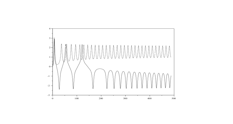
Figure 2.22: Evolution of the mean value $\bar{\phi}$ for $\lambda=0.1$ and for two different initial conditions: $\bar{\phi}=0.08$ (solid line) and $\bar{\phi}=0.16$ (dashed line), with the “flipped” choice for the spinodal modes.

Figure 2.23: Evolution of the mean value $\bar{\phi}$ for $\lambda=0.1$, with $\bar{\phi}(t=0)=0.08$, and two different initial conditions for the quantum spinodal modes, “flipped” (solid line) and massless (dashed line).

Figure 2.24: Asymptotic values of the mean field $\bar{\phi}$, plotted vs. initial values $\bar{\phi}(t=0)$, for $\lambda=0.1$.

Figure 2.25: Comparison between the classical energies for the two initial conditions of Fig 2.22.

Figure 2.26: Evolution of the condensate $\bar{\phi}$ (solid line) and of the corresponding classical energy (dashed line), for $\bar{\phi}(t=0)=0.16$ and $\lambda=0.1$ (cfr. Fig.s 2.25 and 2.22).

Figure 2.27: Evolution of the condensate $\bar{\phi}$ (solid line) and of the corresponding classical energy (dashed line), for $\bar{\phi}(t=0)=0.08$ and $\lambda=0.1$ (cfr. Fig.s 2.25 and 2.22).

Before passing to discuss the influence of different initial conditions on the results, let us present the asymptotic behavior I find when I choose the flipped initial condition. In Fig. 2.24 I have plotted the asymptotic values of the mean field versus the initial values, for $\lambda=0.1$. All dimensionfull quantities are expressed in terms of the suitable power of the equilibrium mass $m$. For example, the vev of the field is equal to $\sqrt{5}$ in these units. First of all, consider the initial values for the condensate far enough from the top of the potential hill, say between $\bar{\phi}(t=0)=0.88$ and $\bar{\phi}(t=0)=2.64$. In that region the crosses seem to follow a smooth curve, that has its maximum exactly at $\bar{\phi}_{\infty}=\sqrt{5}$ (the point of stable equilibrium). When I start from an initial condition smaller than $\bar{\phi}(t=0)=0.88$, the asymptotic value $\bar{\phi}_{\infty}$ is not guaranteed to be positive anymore. On the contrary, it is possible to choose the initial condition in such a way that the condensate will oscillate between positive and negative values for a while, before settling around an asymptotic value near either one or the other minimum, as fig 2.22 clearly shows. Fig.s 2.25, 2.26 and 2.27 helps to understand this behavior by consideration on the energy balance. Both the evolutions are such that the classical energy, defined as $(\dot{\bar{\phi}})^{2}/2+\lambda(\bar{\phi}^{2}-v^{2})/4$, is not a monotonically decreasing function of time. Indeed, energy is continuously exchanged between the classical degree of freedom and the quantum fluctuations bath, in both directions. However, the two rates of energy exchange are not exactly the same and an effective dissipation of classical energy on average can be seen, at long time at least. Of course, this is not the case for the initial transient part of the evolution starting from the initial condition $\bar{\phi}(t=0)=0.08$; there, the condensate absorbs energy (on average) from the quantum fluctuations, being able to go beyond the top of the potential hill, towards the negative minimum. This happens because in case of broken symmetry, the minimization of the fluctuation energy, within microscopic gaussian states, is not possible for initial conditions in the spinodal region [cfr. the discussion about the gap equation (2.174) in section 2.10.3]. After a number of oscillations, the energy starts to flow from the condensate to the quantum bath again (on the average), constraining the condensate to oscillate around a value close to one of the two minima. If we look at fig. 2.24 again, we can find positive asymptotic values as well as negative ones, without a definite pattern, in the whole interval $[0.01,0.8]$. If we start with $0<\bar{\phi}(t=0)<0.01$ we have the slow rolling down, already described in section 2.10.4 and the mean field oscillates around a positive value from the beginning, never reaching negative values. A further note is worth being added here. During the phase of slow rolling down, the evolution is very similar to a symmetric evolution starting from $\bar{\phi}(t=0)=0$; in that case, the dissipation mechanism works through the emission of (quasi-)massless particles and it is very efficient because it has not any perturbative threshold. If the field stays in this slow rolling down phase for a time long enough, it will not be able to absorb the sufficient energy to pass to the other side ever again and it will be confined in the positive valley for ever. Evidently, when $\bar{\phi}(t=0)>0.01$ this dissipative process might not be so efficient to prevent the mean field from sampling also the other valley. Which one of the two valleys will be chosen by the condensate is a matter of initial conditions and it is very dependent from the energy stored in the initial state, as is shown in fig. 2.23, where two evolutions are compared, starting from the same value for the condensate, but with the two initial conditions, “flipped” and massless, for the quantum fluctuations.

2.11 Evolution of a non-homogeneous background

2.11.1 Motivations and summary

To get a better comprehension of the phenomena involved in out of equilibrium phase transitions, like the phase ordering process evolving through the formation of ordered domains separated by domain walls, it would be very useful to be able to follow the history of non–homogeneous condensates, which are large amplitude field configuration localized in space, in interaction with their quantum fluctuations. Defect formation during phase transitions may reveal unifying understanding of phenomena belonging to a wide range of energy scale. In fact, such objects are relevant in condensed matter systems, where the kinks (or solitons) represent charge density waves and conducting polymers, whose transport properties need to be studied in detail. Spatially dependent semiclassical configurations are also important in cosmology and particle physics (electroweak domain walls, called sphaleron, may play a crucial role in understanding electroweak baryogenesis). Also the bubble and droplet nucleation during supercooled phase transitions may be addressed with this formalism. (For a static study of topological defect formation in QFT, with a discussion of finite temperature and volume effects, see also [97]).

Interesting results have been obtained from the analysis of domain walls and kinks out of equilibrium, in model theories like $\lambda\phi^{4}$ and sine–Gordon in $(1+1)-$D dimensions in the dilute regime (which means at a temperature much smaller than the kink’s mass) [98]. The collective coordinate quantization technique at one loop order is used to trace out the meson degrees of freedom and compute the influence functional, which in turn consistently gives the proper Langevin equation. In this scheme, the relaxation is given by the interaction between the domain wall and the meson fluctuations. As a result, the noise is gaussian and additive, although colored and it is related to the damping kernel by a proper fluctuation–dissipation relation. The equations describing the evolution are studied both analytically and numerically and show the presence of a dynamical friction coefficient. It is shown that a Markovian approximation fails to describe the dynamics at large temperatures, the long time relaxation is dominated by classical Landau damping.

With a slightly different approach, a Langevin–like effective equation of motion for the linear $\sigma$ model, was derived in [28], which is valid up to two loops and to $O(\lambda^{2})$. The results for a quartic self interaction are compared to those produced by a quadratic interaction with other fields. The equation describes the evolution towards equilibrium for a non uniform time dependent background field configuration, starting not too far from equilibrium, and is obtained integrating out the faster short wavelength fluctuations. This equation displays noise and dissipation terms which obey a suitable dissipation–fluctuation relation. The noise is in general colored and multiplicative for each finite value of the temperature (the dissipation coefficient depends quadratically on the field amplitude and vanishes in the infinite temperature limit), that is different from the phenomenological Langevin equation usually used with white and additive noise; this may reduce the relaxation time scales and accelerate the approach to equilibrium.

The $O(4)$ linear $\sigma$ model is studied also in connection with the non equilibrium relaxation of an inhomogeneous initial configuration due to quantum and thermal fluctuations. The subject is relevant for the physics of heavy ion collisions, because while the inflaton condensate can be regarded as quasi–uniform due to the exponential expansion, this is not surely the case for the disoriented chiral condensates which may form in present high energy experiments. Indeed, non homogeneous semi–classical configurations will be produced, which will relax through emission of pions in the medium. This will reduce the spatial gradient of the condensates, making the energy decrease. The asymptotic space–time evolution of such configurations is studied in [99], by means of the CTP methods combined with a small amplitude expansion which linearizes the evolution equations in leading order. The relaxation of an initial gaussian inhomogeneous configuration is studied for $\theta\gg\sqrt{t^{2}-r^{2}}$ in terms of the spreading of the packet and of the decay in spherical waves. Different physical situations are considered, and it turns out that at one–loop approximation, the evolution can be described in terms of temperature and a decay rate which depend on rapidity. Moreover, the time scales involved are longer for larger rapidities. At $T\neq 0$ new relaxational processes are found, due to thermal cuts, which do not have counterpart in the homogeneous case.

Spatially dependent configuration are considered also in [93, 94], in the framework of a time dependent variational approach which goes beyond the Gaussian ansatz approximation.

In order to study analytically and numerically the relaxation of a (non perturbative) strongly out of equilibrium inhomogeneous field configuration and the emergence of a hydrodynamical description from ab initio calculation, a self–consistent variational framework which incorporates the quantum back reaction effects and particle production is used in [69]. It is important to get update equations which are renormalizable and local. The renormalization issue is very important, because it guarantees the independence on the size of the spatial greed, while the locality limits the memory requirements on the numerical algorithm. The initial Cauchy data for the inhomogeneous expectation value and for the corresponding Green’s functions is given as a solution of a self–consistent problem, which, for $\phi^{4}$ and sine–Gordon models in $1+1$, is mapped in a Schrodinger like problem by suitable ansatze.

2.11.2 Definitions and preliminaries

I summarize briefly the main definitions and the procedures followed to derive the evolution equations (the interested readers may find useful reading ref. [100] for the rigorous quantization of a field theory on a spherical basis).
I define the expectation values of the field and of its conjugated momentum:

$$\left\langle\hat{\phi}(x)\right\rangle=\phi(x)\;,\qquad\left\langle\hat{\pi}(x)\right\rangle=\pi(x)$$ (2.179)

Then I shift the field operators and I define the fluctuation operators $\eta$ and $\sigma$:

$$\hat{\phi}(x)=\phi(x)+\hat{\eta}(x)\;,\quad\hat{\pi}(x)=\pi(x)+\hat{\sigma}(x)$$ (2.180)

The 2-point functions (equal–time Green’s functions) of the fluctuation operators

$$w(x,y)=\left\langle\hat{\eta}(x)\hat{\eta}(y)\right\rangle{}$$ (2.183)

$${}u(x,y)={\rm Re\,}\left\langle\hat{\eta}(x)\hat{\sigma}(y)\right\rangle=\dfrac{1}{2}\left[\left\langle\hat{\eta}(x)\hat{\sigma}(y)\right\rangle+\left\langle\hat{\sigma}(y)\hat{\eta}(x)\right\rangle\right]{}$$

$${}s(x,y)=\left\langle\hat{\sigma}(x)\hat{\sigma}(y)\right\rangle{}$$

At $N=\infty$ (cfr. [73]) we get the following classical hamiltonian:

$$H=\int d^{\rm d}x\left\{\dfrac{1}{2}\pi^{2}+\dfrac{1}{2}\left|\nabla\phi\right|^{2}+V\left(\phi^{2}+{\rm diag}(w)\right)\right\}{}$$ (2.186)

$${}+\dfrac{1}{2}\int d^{\rm d}x\,d^{\rm d}x^{\prime}\,d^{\rm d}x^{\prime\prime}\,v(x,x^{\prime})w(x^{\prime},x^{\prime\prime})v(x^{\prime\prime},x){}$$

$${}+\dfrac{1}{2}\int d^{\rm d}x\left[\nabla_{\!\!x}\cdot\nabla_{\!\!x^{\prime}}\,w(x,x^{\prime})\bigr{|}_{x=x^{\prime}}+\dfrac{1}{4}\,{\rm diag}(w^{-1})\right]{}$$

The canonical variables enjoy the symplectic structure (cfr. [69, 73, 101]):

$$\left\{\phi_{j}(x),\pi_{k}(x^{\prime})\right\}_{\rm P.B.}=\delta_{jk}\delta^{d}(x-x^{\prime}){}$$ (2.188)

$${}\left\{w(x,y),v(x^{\prime},y^{\prime})\right\}_{\rm P.B.}=\delta^{d}(x-x^{\prime})\delta^{d}(y-y^{\prime})+\delta^{d}(x-y^{\prime})\delta^{d}(y-x^{\prime}){}$$

The Hamilton equations derived for this system can be set in a linear form, that is better implemented numerically, by means of the following conversion from/to canonical variables $w$ and $v$ to/from linear variables $w$, $u$ and $s$:

$$s=\dfrac{1}{4}w^{-1}+vwv+\omega$$ (2.189)

where $\omega$ is a constant ($=0$ for pure states). In addition, we have the relation $u=wv+\omega t$. Thus, we obtain the following linear equations:

$$\begin{array}[]{ll}\dot{\phi}=&\pi\\ \dot{\pi}=&\nabla^{2}\phi-M^{2}\phi\\ \dot{w}=&u+u^{\rm T}\\ \dot{u}=&s+\nabla^{2}_{y}w-M_{y}^{2}w\\ \dot{s}=&\nabla^{2}_{\!\!x}u+\nabla^{2}_{\!\!y}u^{\rm T}-M_{x}^{2}u-M_{y}^{2}u^{\rm T}\end{array}$$ (2.190)

where $M^{2}=2V^{\prime}\left(\phi^{2}+{\rm diag}(w)\right)$ and $M_{x}\equiv M(x)$, $w\equiv w(x,y)\equiv w_{xy}$ and so on.

When the condensate is spherically symmetric, we may assume the quantum state to be rotational invariant, and I may define

$$\phi(x)=\dfrac{1}{\sqrt{4\pi}}\dfrac{\varphi(r)}{r}\;,\quad\pi(x)=\dfrac{1}{\sqrt{4\pi}}\dfrac{p(r)}{r}$$ (2.191)

In addition, I can expand the 2-point functions as follows

$$\Gamma(x,x^{\prime})=\sum_{l=0}^{\infty}\dfrac{2l+1}{4\pi\,rr^{\prime}}\;{\rm P}_{l}(\cos\theta)\,\Gamma^{(l)}(r,r^{\prime})$$ (2.192)

having defined $rr^{\prime}\cos\theta=x\cdot x^{\prime}$, where $\Gamma$ is any of the 2-point functions $w$, $v$, $u$ or $s$. As usual, the boundary conditions at $r=0$ are

$$\varphi(0)=0=p(0)\;,\quad\Gamma^{(l)}(0,r^{\prime})=\Gamma^{(l)}(r,0)=0$$ (2.193)

In case of a sphere of finite volume, with radius $R$, suitable boundary conditions (Dirichlet, von Neumann) can be assumed also at $r=R$. The coincidence limit for $w$ reads:

$${\rm diag}(w)(r)=w(x,x)=\sum_{l=0}^{\infty}\dfrac{2l+1}{4\pi\,r^{2}}w^{(l)}(r,r)$$ (2.194)

Recalling the useful relation (with $r_{i}r_{j}\cos\theta_{ij}=x_{i}\cdot x_{j}$)

$$\int d\Omega_{2}{\rm P}_{l}(\cos\theta_{12}){\rm P}_{l^{\prime}}(\cos\theta_{23})=\dfrac{2l+1}{4\pi}\delta_{ll^{\prime}}{\rm P}_{l}(\cos\theta_{13})$$ (2.195)

I can write, for instance

$$\int d^{3}x_{2}d^{3}x_{3}v(x_{1},x_{2})w(x_{2},x_{3})v(x_{3},x_{4})={}$$ (2.197)

$${}\sum_{l=0}^{\infty}\dfrac{2l+1}{4\pi\,r_{1}r_{4}}{\rm P}_{l}(\cos\theta_{14})\int dr_{2}dr_{3}v^{(l)}(r_{1},r_{2})w^{(l)}(r_{2},r_{3})v^{(l)}(r_{3},r_{4}){}$$

Thus, it is easy to show that in case of rotational invariance the Hamiltonian can be written as

$$H=\int dr\left\{\dfrac{1}{2}p^{2}+\dfrac{1}{2}(\partial_{r}\varphi)^{2}+4\pi r^{2}V\left(\phi^{2}+{\rm diag}(w)\right)\right\}{}$$ (2.199)

$${}+\dfrac{1}{2}\sum_{l=0}^{\infty}(2l+1)\int dr\left\{\left[s^{(l)}(r,r)+\left(-\partial_{r}^{2}+{\textstyle{l(l+1)\over r^{2}}}\right)w^{(l)}(r,r^{\prime})\bigr{|}_{r=r^{\prime}}\right]\right\}{}$$

while the evolution equations in case of rotational invariance read:

$$\begin{array}[]{ll}\dot{\varphi}=&p\\ \dot{p}=&D^{(0)}\varphi\\ \dot{w}^{(l)}=&u^{(l)}+u^{(l)T}\\ \dot{u}^{(l)}=&s^{(l)}+D^{(l)}_{r^{\prime}}w^{(l)}\\ \dot{s}^{(l)}=&D^{(l)}u^{(l)}+\left(D^{(l)}u^{(l)}\right)^{T}\end{array}$$ (2.200)

where

$$D^{(l)}=\dfrac{\partial^{2}}{\partial r^{2}}-\dfrac{l(l+1)}{r^{2}}-M(r)^{2}$$ (2.201)

If I want to consider $\Phi^{4}$ model, I should specify the suitable potential, which is $V(z)=1/2m^{2}_{\rm b}z+\lambda_{\rm b}/4z^{2}$.

Discretized equations
With an eye to the numerical calculation, that will have to be done on a computer, I set up a spatial (radial) lattice with spacing $a$ from $0$ to $R=(N+1)a$, so that the total number of sites is $N+2$. However, due to Dirichelet’s boundary conditions, the two boundary sites (i.e. $0$ and $N+1$, are not linked to dynamical variables). Thus, in this case the background field is a vector $\varphi_{j}=\varphi(ja)$ and the 2-point functions are standard matrices $\Gamma_{ij}=\Gamma(ia,ja)$, with $i,j=0,\cdots,N$. The discretized version for the second derivative is the standard one: $\dfrac{\partial^{2}}{\partial r^{2}}\varphi(r)\bigr{|}_{r=ja}=(\varphi_{j+1}-2\varphi_{j}+\varphi_{j-1})/a^{2}$. The square effective mass becomes:

$$M_{j}^{2}=m^{2}_{\rm b}+\dfrac{\lambda_{\rm b}}{4\pi j^{2}a^{2}}\left[\varphi_{j}^{2}+\sum_{l=0}^{\infty}(2l+1)w^{(l)}_{jj}\right]$$ (2.202)

Now I can try to use the fourth–order Runge-Kutta algorithm (already used in the homogeneous case) to solve this system of coupled ordinary differential equations.

Initial conditions
I can fix the initial conditions in the following way: I start with an arbitrary profile for $\varphi(r)$ and with $p(r)=0$; then I want to find suitable initial conditions for the 2-point functions. One possible choice is to minimize the energy functional with respect to the fluctuations. This is achieved first by setting $v(x,y)=0$; in that case, also $u(x,y)$ is $0$; then I must find some minimal $w^{(l)}(r,r^{\prime})$. From the numerical point of view, I may choose two possible strategies in order to solve this problem:
1) one might try to solve the non–linear differential equations for $w^{(l)}$:

$$s^{(l)}(r,r^{\prime})+\left[\dfrac{\partial^{2}}{\partial r^{2}}-\dfrac{l(l+1)}{r^{2}}-M(r)^{2}\right]w^{(l)}(r,r^{\prime})=0$$ (2.203)

where now

$$\int drs^{(l)}(r,r^{\prime})w^{(l)}(r^{\prime},r^{\prime\prime})=\dfrac{1}{4}\delta(r-r^{\prime\prime})$$ (2.204)

2) otherwise, one may try to minimize directly the energy functional (2.199), using numerical algorithms like the Simplex, Conjugated Gradient or Simulated Annealing methods.

Free Massive Scalar Field
To clarify matters, especially with respect to the renormalization issue, let us compute the expansion in partial waves of the Green function $w(x,y)$ for a free massive scalar field and check that its spherical components $w^{(l)}$ satisfy the equations (2.203).

$$w_{0}(x_{1},x_{2};m)=w_{0}(x_{1}-x_{2};m)=\dfrac{1}{2}\int\dfrac{d^{3}k}{(2\pi)^{3}}\dfrac{e^{\imath k\cdot(x_{1}-x_{2})}}{\sqrt{k^{2}+m^{2}}}$$ (2.205)

This integral can be computed in closed form

$$w_{0}(r_{12};m)=\dfrac{m}{4\pi^{2}r_{12}}K_{1}(mr_{12})=\dfrac{1}{4\pi^{2}r_{12}^{2}}+\dfrac{m^{2}}{8\pi^{2}}\ln(mr_{12})+{\rm finite}$$ (2.206)

where the coincidence limit singularities are made explicit.
Let us use a Dirac formalism to indicate the simultaneous eigenstates of the operators $|\boldsymbol{P}|$, $\boldsymbol{L}^{2}$ and $\boldsymbol{L}_{z}$:

$$\left\langle x\right|\left.k,l,m\right\rangle=\sqrt{\dfrac{2}{\pi}}j_{l}(kr)Y_{lm}(\hat{x})$$ (2.207)

that satisfy the orthogonality and closure rule

$$\left\langle k,l,m\right|\left.k^{\prime},l^{\prime},m^{\prime}\right\rangle=\dfrac{1}{k^{2}}\delta(k-k^{\prime})\delta_{ll^{\prime}}\delta_{mm^{\prime}}{}$$ (2.209)

$${}\sum_{l.m}\int dkk^{2}\left|k,l,m\right\rangle\left\langle k,l,m\right|={\rm Id}{}$$

The following identities hold:

$$\sum_{l,m}Y_{lm}(\hat{x}_{1})Y_{lm}(\hat{x}_{2})=\sum_{l}\dfrac{2l+1}{4\pi}P_{l}(\cos\theta_{12})=\delta^{(2)}(\hat{x}_{1}-\hat{x}_{2}){}$$ (2.211)

$${}\int dr\,r^{2}j_{l}(k_{1}r)j_{l}(k_{2}r)=\dfrac{\pi}{2}\dfrac{1}{k_{1}^{2}}\delta(k_{1}-k_{2}){}$$

Using the partial wave expansion of the plane wave and after some algebra I end up with

$$w_{0}(x_{1},x_{2};m)=\sum_{l}\dfrac{2l+1}{2\pi^{3}}P_{l}(\cos\theta_{12})\int dkk^{2}\dfrac{j_{l}(kr)j_{l}(kr^{\prime})}{2\sqrt{k^{2}+m^{2}}}$$ (2.212)

from where I can read the explicit expression of $w^{(l)}$:

$$w_{0}^{(l)}(r,r^{\prime};m)=\dfrac{2}{\pi^{2}}rr^{\prime}\int_{0}^{\Lambda}dkk^{2}\dfrac{j_{l}(kr)j_{l}(kr^{\prime})}{2\sqrt{k^{2}+m^{2}}}\;,\quad\Lambda\to\infty$$ (2.213)

For example, the integral for $l=0$ can be computed exactly in terms of the Bessel $K_{0}$:

$$w_{0}^{(0)}(r,r^{\prime};m)=\dfrac{1}{2\pi^{2}}\left[K_{0}(m|r-r^{\prime}|)-K_{0}(m(r+r^{\prime})\right]$$ (2.214)

The spherical components of $w^{-1}$ are given by:

$$w_{0}^{(l)-1}(r,r^{\prime};m)=\dfrac{2}{\pi^{2}}rr^{\prime}\int dkk^{2}2\sqrt{k^{2}+m^{2}}j_{l}(kr)j_{l}(kr^{\prime})$$ (2.215)

One can easily verify that $w^{(l)}$ is a solution of the self-consistent equation (2.203); in fact, the spherical Bessel functions $j_{l}(kr)$ are eigenfunctions of the Bessel operator

$$\left(-\partial_{r}^{2}+\dfrac{l(l+1)}{r^{2}}\right)[rj_{l}(kr)]=k^{2}[rj_{l}(kr)]$$ (2.216)

Let us now consider the Hamiltonian (2.199). For a free massive scalar field, the potential reduces to the form:

$$\dfrac{m^{2}}{2}\sum_{l}(2l+1)\int drw_{0}^{(l)}(r,r;m)$$ (2.217)

that can be written as

$$m^{2}\int\dfrac{dk}{\pi}\dfrac{k^{2}}{2\sqrt{k^{2}+m^{2}}}\int drr^{2}\sum_{l}\dfrac{2l+1}{\pi}j_{l}^{2}(kr)$$ (2.218)

The (functional) series in the internal integral is a constant exactly equal to $1/2$ (cfr. [102], 8.536 1., page 980); thus I am left with the integral on the quantum fluctuations times a volume factor, due to translation invariance

$$\sum_{l}(2l+1)\int dr\,w_{0}^{(l)}(r,r;m)=V\int\dfrac{d^{3}k}{(2\pi)^{3}}\dfrac{1}{2\sqrt{k^{2}+m^{2}}}$$ (2.219)

In other words, the volume factor can be written as

$$\delta^{(3)}(k)\bigr{|}_{k=0}=\dfrac{V}{(2\pi)^{3}}=\sum_{l}\dfrac{2l+1}{2\pi^{3}}\int drr^{2}j_{l}^{2}(kr)$$ (2.220)

Renormalization
The coincidence limit of the 2-point function yields ultraviolet divergences that must be properly subtracted before solving the evolution equations numerically. I consider the case of unbroken symmetry for simplicity. The space-time dependent effective mass must be written in terms of finite quantities, and this set our renormalization conditions. First, I parametrize $m^{2}_{\rm b}$ using the equilibrium free field 2-point function for a massive field of renormalized mass $m$:

$$m^{2}_{\rm b}=m^{2}-\lambda_{\rm b}{\rm diag}(w_{0})=m^{2}-\lambda_{\rm b}\sum_{l}\dfrac{2l+1}{4\pi r^{2}}w^{(l)}_{0}(r,r;m)$$ (2.221)

where $w^{(l)}_{0}(r,r^{\prime})$ is given by eq. (2.213). When the sum over $l$ runs from $0$ to $\infty$, the complete free ultraviolet divergence is correctly rebuilt:

$$\left({\rm diag}(w_{0})\right)(r)=\int_{0}^{\Lambda}dk\,\dfrac{k^{2}}{2\sqrt{k^{2}+m^{2}}}\sum_{l}\dfrac{2l+1}{2\pi^{3}}j_{l}(kr)^{2}=\int_{0}^{\Lambda}dk\,\dfrac{k^{2}}{2\sqrt{k^{2}+m^{2}}}$$ (2.222)

I still have a logarithmic divergence, due to the difference $M(r)^{2}-m^{2}$, which I absorb in the definition of the renormalized coupling $\lambda$:

$$M(r)^{2}=m^{2}+\lambda\left[\phi(x)^{2}+{\rm diag}(w)_{\rm R}\right]{}$$ (2.224)

$$={}m^{2}+\dfrac{\lambda_{\rm b}}{4\pi r^{2}}\left\{\varphi(r)^{2}+\sum_{l=0}^{l_{\rm max}}(2l+1)\left[w^{(l)}(r,r)-w^{(l)}_{0}(r,r;m)\right]\right\}{}$$

When I stop the sum over the partial waves at a finite $l_{\rm max}$, I should subtract the ultraviolet divergences before performing the sum. The partial waves $w^{(l)}_{0}(r,r;m)$ should be computed once and for all at the beginning, performing the integral (2.213) for the values of $r$ corresponding to the lattice chosen and with an upper momentum cut-off equal to $\pi/a$. It should be recalled that, for fixed $l$, each $w^{(l)}_{0}(r,r;m)$ has only a logarithmic divergence in the ultraviolet cut-off $\Lambda$, as can be easily inferred expanding for large arguments the spherical Bessel function in eq. (2.213), plus finite parts that do depend on $r$. Thus, subtracting the divergence for each $l$ before performing the sum could be quantitatively very different (for given $l_{\rm max}$, $\Lambda$ and $R$) from subtracting beforehand the entire constant $\left({\rm diag}(w_{0})\right)$:

$$M^{2}(r)=m^{2}+\lambda_{\rm b}\left[\phi(x)^{2}+\sum_{l=0}^{l_{\rm max}}\dfrac{2l+1}{4\pi r^{2}}w^{(l)}(r,r)-{\rm diag}(w_{0})\right]$$ (2.225)

With the subtraction scheme as in (2.224), the functional gap equation

$$M(r)^{2}=m^{2}+\dfrac{\lambda_{\rm b}}{4\pi r^{2}}\left\{\varphi(r)^{2}+\sum_{l=0}^{l_{\rm max}}(2l+1)\left[w^{(l)}(r,r)-w^{(l)}_{0}(r,r;m)\right]\right\}{}$$ (2.226)

$${}\left[-\dfrac{\partial^{2}}{\partial r^{2}}+\dfrac{l(l+1)}{r^{2}}+M(r)^{2}\right]w^{(l)}(r,r^{\prime})=\dfrac{1}{4}w^{(l)\,-1}(r,r^{\prime}){}$$

that determine the initial conditions, trivially admits the equilibrium solution $\phi=0$, $M(r)^{2}=m^{2}$, $w^{(l)}=w_{0}^{(l)}$. Eq. (2.226) is formally solvable via mode expansion: suppose we have the complete solution of the eigenvalue problem

$$\left[-\dfrac{\partial^{2}}{\partial r^{2}}+U_{l}(r)\right][r\chi^{(l)}_{k}(r)]=k^{2}[r\chi^{(l)}_{k}(r)]$$ (2.227)

where $U_{l}(r)=l(l+1)/r^{2}+M(r)^{2}-m^{2}$ cannot be negative since $M(r)^{2}>m^{2}$ for unbroken symmetry and is assumed to vanish for large $r$ fast enough; then

$$w^{(l)}(r,r^{\prime})=\dfrac{2}{\pi}rr^{\prime}\int_{0}^{\Lambda}dk\,k^{2}\dfrac{\chi^{(l)}_{k}(r)\chi^{(l)}_{k}(r^{\prime})}{2\sqrt{k^{2}+m^{2}}}$$ (2.228)

and the gap equation reads

$$M(r)^{2}=m^{2}+\dfrac{\lambda_{\rm b}}{4\pi}\left\{\varphi(r)^{2}+\sum_{l=0}^{l_{\rm max}}(2l+1)\int_{0}^{\Lambda}dk\,k^{2}\dfrac{\chi^{(l)}_{k}(r)^{2}-j_{l}(kr)^{2}}{2\sqrt{k^{2}+m^{2}}}\right\}$$ (2.229)

Chapter 3 Out of Equilibrium Dynamics for the Non linear $\sigma$-model in $2D$

3.1 Motivations

As we have seen, much work has been done about the quantum evolution out of equilibrium of the $\phi^{4}$ model in $3+1$ dimensions [52, 53, 55, 59, 61, 85]. As is well known [14], the renormalized theory is trivial. Practically, this means that we should consider the model as an effective theory, keeping the ultraviolet cut-off $\Lambda$ much smaller than some Landau scale. The logarithmic dependence on $\Lambda$ should disappear from the renormalized quantities, while a weak inverse power dependence remains.

If we want to push the application of non equilibrium techniques to more fundamental theories, like QCD, we should consider that the ultraviolet properties change drastically. In those cases, in fact, there is no Landau Pole in the ultraviolet and the renormalized coupling becomes smaller and smaller as the momentum scale increases. This corresponds to the property of asymptotic freedom, whose presence justifies self–consistently the perturbative renormalization procedure and allows in principle to perform the infinite cut-off limit smoothly.

Motivated by this consideration, I analyze in this chapter the dynamical properties of the $O(N)$ non linear $\sigma$ model in $1+1$ dimensions and in the large $N$ limit.

The linear and non linear $\sigma$ models in $3+1$ dimensions were introduced in elementary particle theory in order to provide a useful model of the low–energy strong interaction sector, which was able to realize the $SU(2)\times SU(2)$ current algebra and the Partial Conservation of Axial Current (PCAC) and satisfy the corresponding low energy theorems [67]. Afterwards, the non linear $\sigma$ model has been considered fruitfully in many areas of Quantum Field Theory and Statistical Mechanics, mainly in the description of $2D$ spin chains and, quite recently, of disordered conductors and of quantum chaos [103].

For the sake of completeness, I should say that the classical non-linear $\sigma$ model in the large $N$ limit and in $3+1$ dimensions, has been used for the study of the phase ordering dynamics in a FRW background, revealing the existence of scaling solutions of the classical field equations [104, 105, 106]. However, in that case the main disadvantages are that one looses the renormalizability and is constrained to stay at the classical level.

As is well known, the theory in $(1+1)$D is renormalizable and asymptotically free in the ultraviolet [89]. Thus, $\Lambda$ can be pushed to infinity rigorously and there should exist a renormalized out–of–equilibrium dynamics, completely independent of the ultraviolet cut-off.

It is very important to study and understand the scaling properties of the dynamics with respect to the ultarviolet cutoff $\Lambda$. In the case of the trivial linear model, in fact, $\Lambda$ should be kept in any case much smaller than the Landau pole. If it is also taken bigger than the largest unstable mode, the corresponding dynamics is quite insensitive to the specific value of $\Lambda$ chosen, because once the whole unstable band has been included, making $\Lambda$ bigger means adding only oscillating perturbative modes. In the case of the non linear model, instead, there is not any instability and the effect of a bigger number of modes should be checked carefully.

To get the non linear model at leading order in $1/N$ I will have to perform two limits: the limit $N\to\infty$ and the limit of large coupling which enforces the constraint. While it is not clear, a priori, that these two limits commute, I give here a rigorous proof that this is, in fact the case. Thus, the non linear model at $N=\infty$ is uniquely defined.

3.2 The model in $0+1$ dimensions

In this section I rigorously prove the commutativity of the two limits in the simple case of the quantum mechanics constrained on the sphere.

I first set $N=1$ and I choose a symmetry breaking potential $V$ of the form:

$$V\left(x\right)=\dfrac{\lambda}{4!}\left(x^{2}-v^{2}\right)=\dfrac{1}{2}\mu^{2}x^{2}+\dfrac{\lambda}{4!}x^{4}+\dfrac{3\mu^{4}}{2\lambda}$$ (3.1)

where I identify $v^{2}$ with $-6\mu^{2}/\lambda$. Now, it is not difficult to see that if I perform the limit $\lambda\rightarrow\infty$, keeping $v^{2}$ fixed, also the second derivative of the potential at the two minima tends to infinity, meaning that at the classical level, the variable $x$ is constrained to assume only values compatible with $x^{2}=v^{2}$. It is straightforward to treat the vector model ($N>1$), the only change being transformation of $x$ to a $N$–component vector.

Now I derive the quantum dynamics in the large $N$ limit, applying a general technique already used in the analysis of the $\phi^{4}$ dynamics in finite volume [80] and based on well–known work by Yaffe [73]. Consider the quantum mechanical system described by the potential (3.1). The corresponding hamiltonian is $\hat{H}=\hat{p}^{2}/2+V(\hat{q})$. Performing first the large $N$ limit, I get the classical hamiltonian

$$h^{(u)}=\dfrac{1}{2}p^{2}+\dfrac{1}{2}s^{2}+\dfrac{1}{8\sigma^{2}}+V\left(q^{2}+\sigma^{2}\right)$$ (3.2)

Where $q$ is now the average value and $\sigma$ is the width (the quantum fluctuation) of the position operator, and $p$ and $s$ are related to the corresponding quantities for the momentum operator. If I use the potential $V$ to enforce the constraint (i.e. $\lambda\to\infty$, keeping $v^{2}$ fixed), I get the quantum constraint $q^{2}+\sigma^{2}=v^{2}$.

This last result deserves a more detailed comment: we see that while at the classical level the $x$-variable lives on the iper-sphere exactly, the mean value of the quantum operator $\hat{q}$ can assume values inside the iper-sphere and not only on its surface, thanks to the presence of the quantum fluctuations. On the other hand, in analyzing the quantum model, we should think in terms of wave functions on the sphere, whose square modulus represents a density probability for a precise unitary vector. On this basis, the mean value should be understood as a continuum weighted sum (integral) of vectors, divided by a suitable normalization and nothing prevents it to be different from $v$; actually, it may assume any value in the interval $\left[0,v\right]$, $q=0$ corresponding to the spherically symmetric state, where all the directions have the same weight. In this case the wave function is uniform on the iper-sphere (it is $Y_{00}$ in the language of the 3-D spherical harmonics).

If I perform the Legendre transform on (3.2), I obtain the corresponding classical Lagrangian, in terms of the constrained variables $\left(q,\sigma\right)$ and their time first derivatives. I now define the projective coordinate $\tau$:

$$q=\dfrac{1-\tau^{2}}{1+\tau^{2}}\,\,\,\sigma=\dfrac{2\tau}{1+\tau^{2}}$$

its conjugated momentum $T$

$$p=-\tau T\,\,\,s=\dfrac{T}{2}\left(1-\tau^{2}\right)$$

and I obtain the hamiltonian in terms of unconstrained canonically conjugated variables:

$$h=\dfrac{1}{8}\left(1+\tau^{2}\right)^{2}\left(T^{2}+\dfrac{1}{4\tau^{2}}\right)$$ (3.3)

Let us now see what happens if I take the two limits in the reversed order. In order to do that I must first define what I mean by quantum mechanics on the sphere $S^{N}$.

Let us consider a sphere of radius $R$ in the vector space $R^{N+1}$, defined by the implicit equation:

$$\sum_{i=1}^{N+1}x_{i}^{2}=R^{2}$$

The projective coordinates are defined by:

$$x_{i}=\dfrac{2\alpha_{i}/R}{1+\alpha\cdot\alpha/R^{2}}\,\,\,x_{N+1}=\dfrac{\alpha\cdot\alpha/R^{2}-1}{1+\alpha\cdot\alpha/R^{2}}$$

The metric on the sphere in the projective coordinates is given by:

$$g_{jk}=\Omega^{2}\delta_{jk}\;\quad\rm{with}\;\Omega=\dfrac{2}{1+\alpha\cdot\alpha/R^{2}}$$

I define the hamiltonian for the free motion as the Laplacian operator on the sphere

$$\bigtriangleup=-\dfrac{1}{\sqrt{g}}\partial_{j}\sqrt{g}g^{jk}\partial_{k}=-\Omega^{-N}\partial_{j}\Omega^{N-2}\partial_{j}$$ (3.4)

I neglect, here, a possible term proportional to the scalar curvature, because in the case of the sphere it is a constant and it modifies the spectrum only additively.

I can choose two different representations of the Hilbert Space of the system: either

$${\cal L}_{2}\left(R^{N};d\mu=\Omega^{N}d^{N}\alpha\right)$$

or

$${\cal L}_{2}\left(R^{N};d\mu_{0}=d^{N}\alpha\right)$$

The Laplacian in the second representation is given by

$$\overline{\bigtriangleup}=\Omega^{N/2}\bigtriangleup\Omega^{-N/2}=-\dfrac{1}{2}\left(\Omega^{-2}\partial^{2}+\partial^{2}\Omega^{-2}\right)+\left(\dfrac{1}{2}+\dfrac{2}{N}\right)\dfrac{\alpha\cdot\alpha}{N}-\dfrac{N}{4}+1$$

where I have set $R=\sqrt{N}$ in order to implement the large $N$ limit. I can express the result in terms of the Yaffe operators [73]:

$$\dfrac{\alpha\cdot\alpha}{N}=2A\,\,\,-\dfrac{\partial^{2}}{N}=2C$$

to obtain the classical hamiltonian describing the large $N$ limit:

$$h=\dfrac{1}{8}\left(1+\tau^{2}\right)^{2}\left(T^{2}+\dfrac{1}{4\tau^{2}}\right)$$ (3.5)

Being this the same result obtained previously, it proves the commutativity of the two limits.

In conclusion, I managed to show, in this very specific case (large $N$ limit of the $O\left(N\right)$ non-linear $\sigma$ model), that the quantization procedure commutes with the implementation of the constraint.

It is worth noticing that the formalism can be extended to include also mean value vectors pointing in arbitrary directions and having $n$ components.

3.3 The $O(\infty)$ non linear $\sigma$ model in $1+1$ dimensions

3.3.1 Definitions

The classical Lagrangian of the $O(N+1)$ $\sigma$ model is given by

$$L=\dfrac{1}{2}\,\partial_{\mu}\boldsymbol{\phi}\cdot\partial_{\mu}\boldsymbol{\phi}$$ (3.6)

Where $\boldsymbol{\phi}$ is a multiplet transforming under the fundamental representation of $O(N+1)$ and constrained to the $N-$dimensional sphere of radius $\lambda^{-1/2}$:

$$\phi^{2}\equiv\boldsymbol{\phi}\cdot\boldsymbol{\phi}=1/\lambda$$ (3.7)

$\lambda$ may be regarded as the coupling constant, since the sphere flattens out in the $\lambda\to 0$ limit. The Hamiltonian corresponding to (3.6) reads

$$H=\dfrac{1}{2}\int dx\left[J^{2}+(\partial_{x}\phi)^{2}\right]\;,\quad J^{2}=\sum_{i<j}J_{ij}^{2}$$ (3.8)

where $J_{ij}=\phi_{i}\pi_{j}-\phi_{j}\pi_{i}$ is the angular momentum on the sphere, $\pi_{j}$ being the momentum conjugated to $\phi_{j}$. This Hamiltonian can also be obtained as the $g\to\infty$ limit of the linear model

$$H_{\rm L}=\int dx\left[\dfrac{1}{2}\pi^{2}+\dfrac{1}{2}(\partial_{x}\phi)^{2}+V(\phi^{2})\right]$$ (3.9)

where $\boldsymbol{\phi}$ is now unconstrained and the potential $V$ may be taken of the form

$$V(u)=\dfrac{g}{4}(u-1/\lambda)^{2}$$ (3.10)

The quantum version of the linear model defines a textbook Quantum Field Theory (apart from the nontrivial strong coupling limit $g\to\infty$). The quantum version of the nonlinear model (3.8) may be written instead

$$H=\dfrac{1}{2}\int dx\left[-\bigtriangleup+\,\omega^{2}\,(\partial_{x}\alpha)^{2}\right]$$ (3.11)

where I have used the projective coordinates $(\alpha_{1},\ldots,\alpha_{N})$ on the sphere, namely

$$\phi_{j}=\omega\,\alpha_{j}\;,\quad\lambda_{\rm b}^{1/2}\phi_{N+1}=\omega-1\;,\quad\omega=\dfrac{2}{1+\lambda_{\rm b}\alpha^{2}}$$ (3.12)

so that

$$(\partial_{x}\phi)^{2}=\omega^{2}\,(\partial_{x}\alpha)^{2}$$ (3.13)

and the $O(N+1)-$symmetric functional Laplacian reads

$$\bigtriangleup(x)=\omega(x)^{-N}\dfrac{\delta}{\delta\alpha_{j}(x)}\,\omega(x)^{N-2}\,\dfrac{\delta}{\delta\alpha_{j}(x)}$$ (3.14)

I have replaced the coupling constant $\lambda$ with $\lambda_{\rm b}$ (the bare coupling constant) to stress the fact that in Quantum Field Theory it is generally cut-off dependent.

3.3.2 The $N\to\infty$ limit

If we consider the non linear model as a limit of the $\phi^{4}$ linear model (being this true at least at the classical level), we have to take two limits and we might wonder whether it is legitimate to interchange their order. To be more specific, if I first perform the large $N$ limit in the linear model, I get a classical $g-$dependent unconstrained Hamiltonian $H^{\infty}_{\rm L}$, that admits a definite non linear limit $H^{\infty}$ as $g\to\infty$. I verify here that indeed the same Hamiltonian $H^{\infty}$ follows if I start directly form the nonlinear quantum Hamiltonian (3.11) and take the $N\to\infty$ à la Yaffe.

Consider the quantum Hamiltonian of the linear model, with the couplings suitably rescaled to allow the large $N$ limit

$$\hat{H}_{\rm L}=\int dx\left[\dfrac{1}{2}\hat{\pi}^{2}+\dfrac{1}{2}(\partial_{x}\phi)^{2}+V(\hat{\phi}^{2})\right]\;,\quad V(u)=\dfrac{g}{4N}(u-N/\lambda_{\rm b})^{2}$$ (3.15)

According to (a slight extension of) Yaffe’s rules, the quantum dynamics described by the $N\to\infty$ limit of the model is described by a classical Hamiltonian, which is the large $N$ limit of the expectation value of the quantum hamiltonian (3.15) on a set of generalized coherent states, labelled by the parameters defined in eq. (3.19). We end up with the following classical hamiltonian

$$H^{\infty}_{\rm L} = \lim_{N\to\infty}\dfrac{\langle\hat{H}\rangle_{\rm L}}{N}=\int dx\left[\dfrac{1}{2}\pi^{2}+\dfrac{1}{2}(\partial_{x}\phi)^{2}+V(\phi^{2}+w(x,x))\right]$$ (3.16)

$$+ \dfrac{1}{2}\int dx\,dx^{\prime}\,dx^{\prime\prime}\,v(x,x^{\prime})w(x^{\prime},x^{\prime\prime})v(x^{\prime\prime},x)$$ (3.17)

$$+ \int dx\left[\dfrac{1}{8}w^{-1}(x,x)-\dfrac{1}{2}\partial_{x}^{2}w(x,x^{\prime})\bigr{|}_{x^{\prime}=x}\right]\;,\quad V(u)=\dfrac{g}{4}(u-1/\lambda_{\rm b})^{2}$$ (3.18)

where the classical canonical variables are defined as

$$\left\{\begin{array}[]{c}\boldsymbol{\phi}(x)\\ \boldsymbol{\pi}(x)\\ w(x,x^{\prime})\\ v(x,x^{\prime})\end{array}\right\}=\lim_{N\to\infty}\dfrac{1}{N}\left\{\begin{array}[]{c}\sqrt{N}\langle\hat{\boldsymbol{\phi}}(x)\rangle\\ \sqrt{N}\langle\hat{\boldsymbol{\pi}}(x)\rangle\\ \langle\hat{\boldsymbol{\phi}}(x)\cdot\hat{\boldsymbol{\phi}}(x^{\prime})\rangle_{\rm conn}\\ \langle\hat{\boldsymbol{\pi}}(x)\cdot\hat{\boldsymbol{\pi}}(x^{\prime})\rangle_{\rm conn}\end{array}\right\}$$ (3.19)

and the non vanishing Poisson brackets read

$$\left\{\phi_{j}(x)\,,\pi_{k}(x^{\prime})\right\}_{\rm P.B.} = \delta_{jk}\delta(x-x^{\prime})$$ (3.20)

$$\left\{w(x,y)\,,v(x^{\prime},y^{\prime})\right\}_{\rm P.B.} = \delta(x-x^{\prime})\delta(y-y^{\prime})+\delta(x-y^{\prime})\delta(y-x^{\prime})$$ (3.21)

It is understood that the dimensionality of the vectors $\boldsymbol{\phi}(x)$ and $\boldsymbol{\pi}(x)$ is arbitrary but finite [that is, only a finite number, say $n+1$, of pairs $(\hat{\boldsymbol{\phi}}(x)\,,\hat{\boldsymbol{\pi}}(x))$ may take a non vanishing expectation value as $N\to\infty$]. Thus, the index $j$ may run form $1$ to $n+1$, where $n+1$ is the number of field components with non zero expectation value.

The $g\to\infty$ limit on the classical Hamiltonian $H^{\infty}_{\rm L}$ is straightforward and reintroduces the spherical constraint in the new form

$$\sum_{j=1}^{n+1}\phi_{j}^{2}+{\rm diag}(w)=1/\lambda_{\rm b}$$ (3.22)

whose conservation in time implies

$$\boldsymbol{\phi}\cdot\boldsymbol{\pi}+{\rm diag}(wv)=0$$ (3.23)

where I have introduced the condensed notation

$$(ab)(x,y)\equiv\int dz\,a(x,z)\,b(z,y)\;,\quad{\rm diag}(a)(x)\equiv a(x,x)$$ (3.24)

Let us now come back to the quantum Hamiltonian (3.11) of the non-linear model. First of all I perform a similitude transformation of the Laplacian, to cast it in a form suitable for the application of Yaffe’s method:

$$\!\!\!-\overline{\bigtriangleup}=-\omega^{N/2}\bigtriangleup\omega^{-N/2}=\dfrac{1}{2}\left(\omega^{-2}{\hat{\beta}}^{2}+{\hat{\beta}}^{2}\omega^{-2}\right)+\left(\dfrac{1}{2}+\dfrac{2}{N}\right)\dfrac{{\hat{\alpha}}^{2}}{N}-\dfrac{N}{4}+1$$ (3.25)

where $\hat{\alpha}_{j}(x)$ is the obvious multiplication operator and $\hat{\beta}_{j}(x)=-i\delta/\delta\alpha_{j}(x)$ its conjugated momentum. Now, after the rescaling $\lambda_{\rm b}\to\lambda_{\rm b}/N$ in eqs. (3.12), by the usual rules in the $N\to\infty$ limit I obtain the classical Hamiltonian

$$H^{\infty} = \dfrac{1}{2}\int dx\left\{\Omega^{-2}\left[\beta^{2}+{\rm diag}(\chi\eta\chi)+\dfrac{1}{4}{\rm diag}(\eta^{-1})\right]\right.$$ (3.26)

$$+ \left.\Omega^{2}\left[(\partial_{x}\alpha)^{2}+\partial_{x}\partial_{x^{\prime}}\eta(x,x^{\prime})\bigr{|}_{x=x^{\prime}}\right]\right\}$$ (3.27)

where

$$\Omega=\dfrac{2}{1+\lambda_{\rm b}[\alpha^{2}+{\rm diag}(\eta)]}$$ (3.28)

and, just as in eq. (3.19),

$$\left\{\begin{array}[]{c}\boldsymbol{\alpha}(x)\\ \boldsymbol{\beta}(x)\\ \eta(x,x^{\prime})\\ \chi(x,x^{\prime})\end{array}\right\}=\lim_{N\to\infty}\dfrac{1}{N}\left\{\begin{array}[]{c}\sqrt{N}\langle\hat{\boldsymbol{\alpha}}(x)\rangle\\ \sqrt{N}\langle\hat{\boldsymbol{\beta}}(x)\rangle\\ \langle\hat{\boldsymbol{\alpha}}(x)\cdot\hat{\boldsymbol{\alpha}}(x^{\prime})\rangle_{\rm conn}\\ \langle\hat{\boldsymbol{\beta}}(x)\cdot\hat{\boldsymbol{\beta}}(x^{\prime})\rangle_{\rm conn}\end{array}\right\}$$ (3.29)

are classical canonically conjugated pairs, with Poisson brackets identical to those in eq. (3.20). I take the indices of the classical fields $\boldsymbol{\alpha}$ and $\boldsymbol{\beta}$ to run form 1 to $n$, having assumed that only the first $n$ components of their quantum counterparts may have expectation values of order $\sqrt{N}$.

To show that the classical Hamiltonian $H^{\infty}$ is equivalent to the $g\to\infty$ limit of $H^{\infty}_{\rm L}$, I need only to solve the spherical constraint (3.22) that emerges in that limit. This amounts to the canonical parameterization of the constrained pairs $(\boldsymbol{\phi},\boldsymbol{\pi})$ and $(w,v)$ in terms of the projective ones $(\boldsymbol{\alpha},\boldsymbol{\beta})$ and $(\eta,\chi)$. It reads

$$\phi_{j}=\Omega\,\alpha_{j}\;,\qquad \lambda_{\rm b}^{1/2}\phi_{n+1}=\Omega-1$$ (3.30)

$$\pi_{j}=\Omega^{-1}\beta_{j}+\alpha_{j}\pi_{n+1}\;,\qquad \pi_{n+1}=-\boldsymbol{\alpha}\cdot\boldsymbol{\beta}-{\rm diag}(\eta\chi)$$ (3.31)

$$w(x,x^{\prime})=\Omega(x)\Omega(x^{\prime})\,\eta(x,x^{\prime})\;,\quad v(x,x^{\prime})=\dfrac{\chi(x,x^{\prime})}{\Omega(x)\Omega(x^{\prime})}+\dfrac{\delta(x-x^{\prime})}{\Omega(x)}\pi_{n+1}(x)$$ (3.32)

and in particular it implies, besides (3.22) and (3.23),

$$\pi^{2}+{\rm diag}(vwv) = \Omega^{-2}\left[\beta^{2}+{\rm diag}(\chi\eta\chi)\right]$$ (3.33)

$$(\partial_{x}\phi)^{2}+\partial_{x}\partial_{x^{\prime}}w(x,x^{\prime})\bigr{|}_{x=x^{\prime}} = \Omega^{2}\left[(\partial_{x}\alpha)^{2}+\partial_{x}\partial_{x^{\prime}}\eta(x,x^{\prime})\bigr{|}_{x=x^{\prime}}\right]$$ (3.34)

This result proves the complete equivalence between the $g\to\infty$ limit on the leading $1/N$ term of the linear model (which imposes the new spherical constraint) and the $N\to\infty$ limit of the quantum model directly formulated on the constraint manifold.

Before closing this section, it should be noticed that, even though I gave the basic definitions and performed the entire computation for a field theory in $1+1$ dimensions, the results in sections 3.3.1 and 3.3.2 remain valid also for a $(D+1)-$dimensional theory, the only change being in the dimensionality of the integrals.

For completeness’ sake I close this section noticing that previous studies this subject (the definition of the non linear quantum model as the large coupling limit of the linear model) were performed in [107], using perturbative techniques and the derivative expansion for the model in 3+1 dimensions. The conclusion was reached that the divergent terms are universal, while finite parts do differs when taking the large coupling limit on the quantum corrections on the linear model, or calculating the same quantum corrections on the nonlinear model.

3.3.3 Dynamical Evolution

Let us now derive the evolution equation for this system in the case the field $\hat{\boldsymbol{\phi}}$ has a non zero, albeit uniform, expectation value $\boldsymbol{\phi}$ in the initial state. The $2-$point functions depend only on the difference $x-x^{\prime}$, and can be parametrized by time–dependent widths $\sigma_{k}$:

$$w(x,x^{\prime})=\int_{-\Lambda}^{\Lambda}\dfrac{dk}{2\pi}\,\sigma_{k}^{2}\,e^{ik(x-x^{\prime})}\;,\quad v(x,x^{\prime})=\int_{-\Lambda}^{\Lambda}\dfrac{dk}{2\pi}\,\dfrac{\dot{\sigma}_{k}}{\sigma_{k}}\,e^{ik(x-x^{\prime})}$$ (3.35)

where $\Lambda$ is the ultraviolet cut-off.

In this case of translation invariance, in practice one can always take $n=1$ owing to the $O(n+1)$ symmetry of $H^{\infty}_{\rm L}$. Thus, I choose $\boldsymbol{\phi}$ to have only two non–zero components. In other words the condensate will move on the plane specified by the initial conditions for $\boldsymbol{\phi}$ and its velocity. Using eq. (3.35), I may write the Lagrangian density corresponding to the ($g\to\infty$ limit) of the Hamiltonian (3.16) as

$$L=\dfrac{1}{2}\left(\dot{\phi}_{1}^{2}+\dot{\phi}_{2}^{2}\right) + \dfrac{1}{2}\int_{-\Lambda}^{\Lambda}\dfrac{dk}{2\pi}\left(\dot{\sigma}_{k}^{2}-k^{2}\sigma_{k}^{2}-\dfrac{1}{4\sigma_{k}^{2}}\right)$$ (3.36)

$$- \dfrac{m^{2}}{2}\left(\phi_{1}^{2}+\phi_{2}^{2}+\int_{-\Lambda}^{\Lambda}\dfrac{dk}{2\pi}\sigma_{k}^{2}-\dfrac{1}{\lambda_{\rm b}}\right)$$ (3.37)

I have kept into account the constraint by introducing the Lagrange multiplier $m^{2}$. The corresponding Euler–Lagrange evolution equations read, in polar coordinates

$$\ddot{\rho}+m^{2}\rho-\dfrac{\ell^{2}}{\rho^{3}}=0$$ (3.38)

$$\ddot{\sigma}_{k}+\left(k^{2}+m^{2}\right)\sigma_{k}-\dfrac{1}{4\sigma_{k}^{3}}=0$$ (3.39)

$$\rho^{2}+\Sigma-\dfrac{1}{\lambda_{\rm b}}=0$$ (3.40)

with the definitions $\ell=\rho^{2}\dot{\theta}$ (the conserved angular momentum of the condensate) and

$$\Sigma={\rm diag}(w)=\int_{-\Lambda}^{\Lambda}\dfrac{dk}{2\pi}\sigma_{k}^{2}$$ (3.41)

The first thing I can do is to look for the minimum of the Hamiltonian, that is the ground state of the theory which corresponds to the vanishing $\ddot{\rho}$, $\dot{\rho}$, $\ddot{\sigma}_{k}$, $\dot{\sigma}_{k}$ and $\ell$. The equations to solve are:

$$m^{2}\rho=0$$ (3.42)

$$(k^{2}+m^{2})\,\sigma_{k}-\dfrac{1}{4\sigma_{k}^{3}}=0$$ (3.43)

The solution $m=0$ is not acceptable, because it yields a massless spectrum for the fluctuations and gives an infrared divergence that violates the constraint. This is nothing else than a different formulation of the well–known Mermin-Wagner-Coleman theorem stating the impossibility of the spontaneous symmetry breaking in $1+1$ dimensions [87, 88]. Thus, the unique solution is: $\rho=0$ and $\sigma_{k}={\textstyle{1\over 2}}(k^{2}+m^{2})^{-1/2}$.

This result allows for an interpretation of the mechanism of dynamical generation of mass as the competition between the energy and the constraint: in order to minimize the “Heisenberg” term in the Hamiltonian, the zero mode width, that is $\sigma_{0}$, should be as large as possible; on the other hand, it cannot be greater than a certain value, because it must also satisfy the constraint. The compromise generates a mass term, the same for all modes, which I call $m_{\rm eq}$

I can take the mass at equilibrium as an independent mass scale defining the theory, as dictated by dimensional transmutation, and the relation between this mass scale and the bare coupling constant is read directly from the constraint (3.40)

$$\dfrac{1}{\lambda_{\rm b}}=\dfrac{1}{2\pi}\log\left(\dfrac{\Lambda}{m_{\rm eq}}+\sqrt{1+\dfrac{\Lambda^{2}}{m_{\rm eq}^{2}}}\right)=\dfrac{1}{2\pi}\log\dfrac{2\Lambda}{m_{\rm eq}}+O\left(\dfrac{m_{\rm eq}^{2}}{\Lambda^{2}}\right)$$ (3.44)

When the system is out of equilibrium, the Lagrange multiplier $m$ may depend on time. Its behavior is determined by the fact that the dynamical variables must satisfy the constraint. After some algebra, this parameter can be written as:

$$m^{2}=\lambda_{\rm b}\left(\dot{\rho}^{2}+\dfrac{\ell^{2}}{\rho^{2}}+\Theta\right)\;,\quad\Theta=\int_{-\Lambda}^{\Lambda}\dfrac{dk}{2\pi}\left(\dot{\sigma}_{k}^{2}-k^{2}\sigma_{k}^{2}+\dfrac{1}{4\sigma_{k}^{2}}\right)$$ (3.45)

I can describe the quantum fluctuations also by complex mode functions $z_{k}$, which are related to the real function $\sigma_{k}$ by:

$$z_{k}=\sigma_{k}e^{i\theta_{k}}\;,\quad\sigma_{k}^{2}\,{\dot{\theta}}_{k}=\ell_{k}=\dfrac{1}{2}\;,\quad\left|\dot{z}_{k}\right|^{2}=\dot{\sigma}_{k}^{2}+\dfrac{\ell_{k}^{2}}{\sigma_{k}^{2}}$$ (3.46)

One can recognize in the second term on the r.h.s. of the last equation in (3.46) the centrifugal energy induced by Heisenberg uncertainty principle.

I choose the following initial conditions for this complex mode functions:

$$z_{k}(0)=\dfrac{1}{\sqrt{2\omega_{k}}}\;,\quad{\dot{z}}_{k}(0)=-i\sqrt{\dfrac{\omega_{k}}{2}}$$ (3.47)

where $\omega_{k}=\sqrt{k^{2}+\alpha^{2}}$ and $\alpha$ is an initial mass scale. It is worth noticing here that such a form for the initial spectrum of the quantum fluctuations does not allow for an initial radial speed for the condensate degrees of freedom, unless I start from $\rho_{0}=0$. This is easily seen by differentiating (3.40) with respect to time.

Moreover, I should stress that $\alpha$ might be different from the initial value of the Lagrange multiplier. In fact, once the initial value for $\rho$ is fixed, $\alpha$ can be determined by means of the constraint equation and it turns out to be

$$\alpha(\rho_{0}) = m_{\rm eq}\exp\left(2\pi\rho_{0}^{2}\right)\left\{\dfrac{1}{2}\left[1+\sqrt{1+\dfrac{m_{\rm eq}^{2}}{\Lambda^{2}}}+\exp(4\pi\rho_{0}^{2})\left(1-\sqrt{1+\dfrac{m_{\rm eq}^{2}}{\Lambda^{2}}}\right)\right]\right\}^{-1}$$ (3.48)

$$= m_{\rm eq}\exp\left(2\pi\rho_{0}^{2}\right)\left[1+O\left(\dfrac{m_{\rm eq}^{2}}{\Lambda^{2}}\right)\right]$$

On the other hand, the initial value for the Lagrange multiplier is given by

$$m^{2}_{0}=\alpha^{2}+\lambda_{\rm b}\left(\dot{\rho}^{2}_{0}+\dfrac{\ell^{2}}{\rho^{2}_{0}}-\alpha^{2}\rho_{0}^{2}\right)$$ (3.49)

that is equal to the initial mass scale $\alpha^{2}$ only if I push the ultraviolet cut–off to infinity.

To properly control for any time the ultraviolet behavior of the integrals in eqs. (3.41) and (3.45), one should perform a WKB analysis [62] of the solution. One finds the following asymptotics for the mode functions:

$$z_{k}(t)=z_{k}(0)\exp\left\{ikt-\dfrac{i}{2k}\int_{0}^{t}dt^{\prime}\,m^{2}(t^{\prime})-\dfrac{1}{4k^{2}}\left[m^{2}(t)-m^{2}(0)\right]\right\}\left[1+O\left(\dfrac{1}{k^{3}}\right)\right]$$ (3.50)

From the above formula it is clear that the logarithmic ultraviolet divergence in $\Sigma$ is completely determined by the initial spectrum. For the divergent integral $\Theta$ in eq. (3.45) the situation is more involved. Explicitly one finds:

$$\Sigma(t)\equiv\int_{-\Lambda}^{\Lambda}\dfrac{dk}{2\pi}|z_{k}(t)|^{2}=\dfrac{1}{2\pi}\log\dfrac{\Lambda}{\mu}+\Sigma_{\rm F}(\mu;t)$$ (3.51)

and

$$\Theta(t)=\int_{-\Lambda}^{\Lambda}\dfrac{dk}{2\pi}\left(|{\dot{z}}_{k}(t)|^{2}-k^{2}|z_{k}(t)|^{2}\right)=m(t)^{2}\,\Sigma(0)+\Theta_{\rm F}(t)$$ (3.52)

where

$$\Sigma_{\rm F}(\mu;t) = \int_{-\Lambda}^{\Lambda}\dfrac{dk}{2\pi}\left[|z_{k}(t)|^{2}-\dfrac{\theta(|k|-\mu)}{2|k|}\right]$$ (3.53)

$$\Theta_{\rm F}(t) = \int_{-\Lambda}^{\Lambda}\dfrac{dk}{2\pi}\left[|{\dot{z}}_{k}(t)|^{2}-k^{2}|z_{k}(t)|^{2}-m(t)^{2}|z_{k}(0)|^{2}\right]$$ (3.54)

have finite limits as $\Lambda\to\infty$. I have introduced in the above formulae a subtraction point $\mu$. There correspond a renormalized coupling constant $\lambda$ running with $\mu$, as the $\Lambda\to\infty$ limit of the relation

$$\dfrac{1}{2\pi}\log\dfrac{\Lambda}{\mu}-\dfrac{1}{\lambda_{\rm b}(\Lambda)}+\dfrac{1}{\lambda(\mu)}=0$$ (3.55)

and a renormalized constraint

$$\rho(t)^{2}+\Sigma_{\rm F}(\mu;t)-\dfrac{1}{\lambda(\mu)}=0$$ (3.56)

With this definitions, the equilibrium mass scale $m_{\rm eq}$ can be written as

$$m_{\rm eq}=2\mu\exp\left[-\dfrac{2\pi}{\lambda(\mu)}\right]$$ (3.57)

which by consistency with eq. (3.48) implies

$$\lambda(\alpha/2)=1/\rho_{0}^{2}$$ (3.58)

In conclusion I can rewrite the constraint and the Lagrange multiplier as

$$\rho^{2}+\Sigma_{\rm F}(\mu)-\dfrac{1}{\lambda(\mu)}=0\;,\quad m^{2}=\dfrac{1}{\rho_{0}^{2}}\left[{\dot{\rho}}^{2}+\dfrac{\ell^{2}}{\rho^{2}}+\Theta_{\rm F}\right]$$ (3.59)

For large but finite UV cutoff these expressions retain a inverse power corrections in $\Lambda$. In the actual numerical calculations whose results will be presented in the following section, I used the “bare” counterparts of eqs (3.59) with finite cutoff and the definition (3.44) of the bare coupling constant is used to reduce to inverse power the cutoff dependence.

Let us conclude this section by summarizing the steps I need to do, before trying to solve numerically the equations of motion. Once I have fixed the UV cutoff, the equilibrium mass scale $m_{\rm eq}$ and the initial value for the condensate $\rho_{0}$, I can determine the initial mass scale $\alpha$ in the fluctuation spectrum from eq. (3.48), which in turn gives the initial conditions for the complex mode functions [cfr. eq. (3.47)]. Now, I need to specify the remaining initial values for the condensate, namely its velocity ${\dot{\rho}}_{0}$ and its angular momentum $\ell$, which must be consistent with the constraint (3.23). Finally, eq. (3.59) completely determines the initial value for the Lagrange multiplier $m_{0}$, which has exactly the same infinite cutoff limit as $\alpha$, but differs significantly from it for finite cutoffs.

I want to stress again the need to consider how the dynamics scales with $\Lambda$, in a theory like this one, which does not show any parametric resonant band (as we will see in the following section). Even though the vanishing of the bare coupling constant should compensate for the increase in the number of modes, when the UV cutoff is increased, it is important to check it explicitly both on the analytic computations and the numerical results.

3.4 Numerical results

I have studied numerically the following evolution equations

$${\ddot{\phi}}+m^{2}\phi=0$$ (3.60)

$${\ddot{z}}_{k}+\left(k^{2}+m^{2}\right)z_{k}=0$$ (3.61)

$$\dfrac{m^{2}}{\lambda_{\rm b}}=|\dot{\phi}|^{2}+\displaystyle{\int_{-\Lambda}^{\Lambda}\dfrac{dk}{2\pi}}\left(|{\dot{z}}_{k}|^{2}-k^{2}|z_{k}|^{2}\right)$$ (3.62)

where $\phi=\phi_{1}+i\phi_{2}=\rho\,e^{i\theta}$, $\rho^{2}\,\dot{\theta}=\ell$ and $|\dot{\phi}|^{2}=\dot{\rho}^{2}+\ell^{2}/\rho^{2}$, while the bare coupling constant $\lambda_{\rm b}$ is given by eq. (3.44). The initial conditions for $\phi$, $\dot{\phi}$ and $z_{k}$ [see eq.s (3.47)] must satisfy the constraints (3.22) and (3.23), that are then preserved by dynamics.

In the classical limit the quantum fluctuations $z_{k}$ disappear from the dynamics. In that case the stationary solutions are trivial:

$$\rho(t)=\lambda_{\rm b}^{-1/2}\;,\quad m(t)=\lambda_{\rm b}\ell$$ (3.63)

with arbitrary value for the angular momentum $\ell$. Thus there are stationary solutions corresponding to circular motion with constant angular velocity.

When I include the coupling with quantum fluctuations, I still obtain stationary solutions, parametrized by $\ell$ which assumes arbitrary positive values. They have the following form:

$$\rho(t)=\sqrt{\dfrac{\ell}{m_{\rm eq}x}}\;\quad\;m(t)=m_{\rm eq}x$$ (3.64)

where $x$ depends on $\ell$ through

$$\dfrac{2\pi\ell}{m_{\rm eq}x}+\sinh^{-1}\left(\dfrac{\Lambda}{m_{\rm eq}x}\right)=\sinh^{-1}\left(\dfrac{\Lambda}{m_{\rm eq}}\right)$$ (3.65)

which reduces to $x\log x=2\pi\ell/m_{\rm eq}$ in the infinite cut–off limit.

3.4.1 Evolution of condensate and Lagrange multiplier

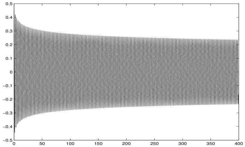
Figure 3.1: Evolution of the mean value $\rho(t)$ for $\Lambda/m_{\rm eq}=10$, $\ell=0$ and $\rho_{0}=0.5$.

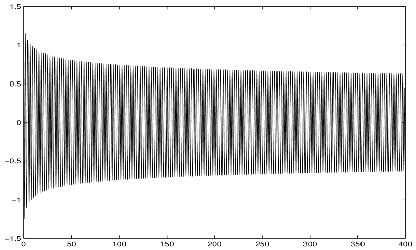
Figure 3.2: Evolution of the mean value speed $\dot{\rho}(t)$ for $\Lambda/m_{\rm eq}=10$, $\ell=0$ and $\rho_{0}=0.5$.

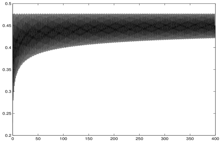
Figure 3.3: Evolution of the backreaction $\Sigma(t)$ for $\Lambda/m_{\rm eq}=10$, $\ell=0$ and $\rho_{0}=0.5$.

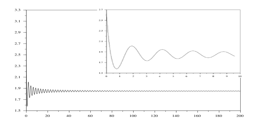
Figure 3.4: Evolution of the Lagrange multiplier $m^{2}(t)$ for $\Lambda/m_{\rm eq}=20$, $\ell=0$ and $\rho_{0}=0.3$. In the smaller figure there is zoom of the early times.

Figure 3.5: Asymptotic evolution of $m^{2}(t)$ for three different values of the ultraviolet cut–off: from top to bottom, $\Lambda/m_{\rm eq}=5,10$ and $20$, $\ell=0$ and $\rho_{0}=0.3$

In order to control the dependence of the dynamics on the ultraviolet cutoff, I solved the equations of motion for values of $\Lambda$ ranging from $5m_{\rm eq}$ to $20m_{\rm eq}$, with an initial condensate ranging from $\rho_{0}=0.2$ to $\rho_{0}=0.7$. I mainly considered the case $\ell=0$. A typical example of the time evolution of the relevant variables is showed in Fig.s 3.1, 3.2 and 3.3. Figure 3.4 shows the evolution of the Lagrange multiplier $m(t)^{2}$ for $\Lambda/m_{\rm eq}=20$; in this case, its starting value is $2.630632$. Due to the lack of massless particles, the damping of the oscillations of $\rho$ and $m^{2}$ is very slow, as already noticed in [55] for the linear model in $1+1$ dimensions; the dissipation is not as efficient as for the unbroken symmetry scenario in $3+1$ dimensions, because of the reduced phase space. A detailed numerical study of the asymptotic behavior and a FFT analysis of the evolution allows a precise determination of the asymptotic value and the main frequency of oscillation of the Lagrange multiplier:

$$m(t)^{2}=m_{\infty}^{2}+\dfrac{p(t)}{t}+O\left(\dfrac{1}{t^{2}}\right)$$ (3.66)

where the function $p(t)$ turns out to be

$$p(t)\simeq A\cos(2m_{\infty}t+\gamma_{1}\log t+\gamma_{2})$$ (3.67)

The logarithmic dependence in the phase could be justified by self–consistent requirements (see below), along the same lines of the detailed calculations performed in ref. [85] in a similar context. Numerically it is very difficult to extract and I do not attempt it here. Comparing further our result with that reported in ref. [85], I should emphasize that I do not find any oscillatory component of frequency $2m_{0}$, as happens instead for the $\phi^{4}$ model in $3+1$ dimensions. Moreover, as figure 3.5 shows, both the asymptotic mass $m_{\infty}$ and the amplitude $A$ depend on the ultraviolet cutoff $\Lambda$. This dependence may be fitted with great accuracy through a low order polynomial in $1/\Lambda^{2}$, showing that the standard renormalization holds at any time, as anticipated by the WKB analysis. Therefore, the extrapolated parameters $m_{\infty}^{2}$ and $A$ give us information on the fully renormalized physical theory (in the large $N$ approximation). The table below collects the values of $m_{\infty}^{2}$ for different values of $\Lambda$ and of the initial condensate $\rho_{0}$. The last column contains the extrapolation to infinite cutoff, obtained by the low order polynomial fit. The empty cells in the last row correspond to a UV cutoff so small that the exact $\alpha^{2}$ turns out to be negative; these values are excluded from the fit.

$\rho_{0}$	$\Lambda=5$	$\Lambda=6$	$\Lambda=7$	$\Lambda=8$	$\Lambda=9$	$\Lambda=10$	$\Lambda=11$	$\Lambda=12$	$\Lambda=13$
$0.2$	$1.3073$	$1.3047$	$1.3032$	$1.3022$	$1.3014$	$1.3010$	$1.3006$	$1.3004$	$1.3001$
$0.3$	$1.8888$	$1.8766$	$1.8693$	$1.8646$	$1.8614$	$1.8591$	$1.8574$	$1.8561$	$1.8551$
$0.4$	$3.3869$	$3.3162$	$3.2747$	$3.2482$	$3.2303$	$3.2175$	$3.2082$	$3.2011$	$3.1956$
$0.5$	$8.7094$	$7.9915$	$7.6082$	$7.3764$	$7.2246$	$7.1193$	$7.0432$	$6.9861$	$6.9424$
$0.6$	$206.03$	$52.433$	$35.564$	$29.2276$	$25.969$	$24.016$	$22.732$	$21.835$	$21.178$
$0.7$									$238.12$

$\rho_{0}$	$\Lambda=14$	$\Lambda=15$	$\Lambda=16$	$\Lambda=17$	$\Lambda=18$	$\Lambda=19$	$\Lambda=20$	$\Lambda=\infty$
$0.2$	$1.300$	$1.2998$	$1.2997$	$1.2996$	$1.2995$	$1.2995$	$1.2994$	$1.2989$
$0.3$	$1.8543$	$1.8536$	$1.8531$	$1.8527$	$1.8523$	$1.8520$	$1.8517$	$1.8493$
$0.4$	$3.1912$	$3.1877$	$3.1848$	$3.1824$	$3.1805$	$3.1788$	$3.1774$	$3.1643$
$0.5$	$6.9080$	$6.8804$	$6.8580$	$6.8395$	$6.8241$	$6.8111$	$6.8001$	$6.6990$
$0.6$	$20.682$	$20.295$	$19.988$	$19.740$	$19.536$	$19.366$	$19.223$	$16.964$
$0.7$	$177.645$	$146.523$	$127.66$	$115.07$	$106.11$	$99.442$	$94.302$	$68.207$

A similar table can be provided for the amplitude $A$ in the eq. (3.67). The values extrapolated to infinite cutoff in a similar fashion as before, turn out to be:

$\rho_{0}$	$0.2$	$0.3$	$0.4$	$0.5$	$0.6$	$0.7$
$A(\Lambda=\infty)$	$0.539$	$0.701$	$0.924$	$1.39$	$2.34$	$4.30$

However, this fit is not as accurate as that for $m_{\infty}$.

It is interesting to observe that at large UV cutoff $m_{\infty}$ has an exponential dependence on $\rho_{0}$ analogous to that of $m_{0}$ (which coincides to $\alpha$ at $\Lambda=\infty$). Most remarkably the prefactor in the exponent is modified by the time evolution: I find

$$m_{\infty}^{2}\sim\exp(2\gamma\,\rho_{0}^{2})\;,\quad 3.5<\gamma<4.5$$ (3.68)

The determination of $\gamma$ is rather rough due to the uncertainties in the values of $m_{\infty}$ extrapolated to $\Lambda=\infty$ at larger $\rho_{0}$. Notice in any case that the analog of $\gamma$ for $m_{0}$ is $2\pi=6.28\ldots$.

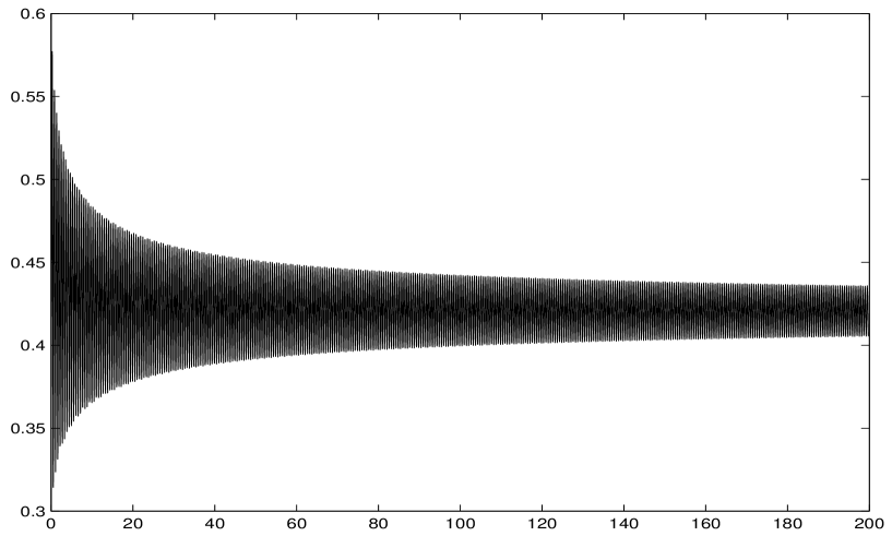
Figure 3.6: Evolution of the mean value $\rho$ for $\Lambda/m_{\rm eq}=10$, $\rho_{0}=0.3$ and $\ell=1$.

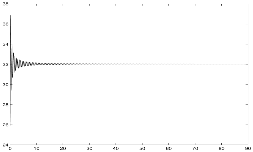
Figure 3.7: Evolution of the squared mass $m^{2}$ for $\Lambda/m_{\rm eq}=10$, $\rho_{0}=0.3$ and $\ell=1$.

I also performed some computations for $\ell>0$, with the following results: if I start from an out of equilibrium value for $\rho$, it will relax through emission of particles towards a fixed point, different from the equilibrium value determined by eq. (3.64). Figures 3.6 and 3.7 show such a situation for $\ell=1.0$, $\rho(0)=0.3$ and $\Lambda=10m_{\rm eq}$. In that case I have $x=1.000057$, while the mean values of the asymptotic oscillations are $\rho_{\infty}=0.4203$ and $m^{2}_{\infty}=32.0294$.

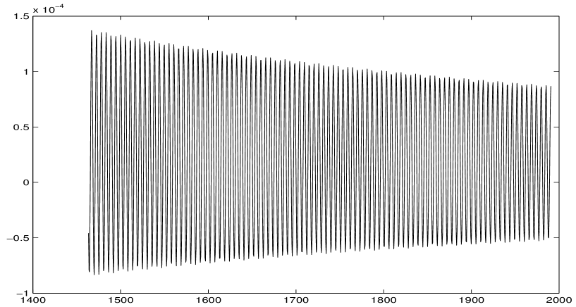
Figure 3.8: The average value of the condensate $\rho$, defined as $\bar{\rho}=\int^{T}\rho(t)dt/T$, plotted vs. $T$, for $\Lambda/m_{\rm eq}=20$, $\ell=0$ and $\rho_{0}=0.2$.

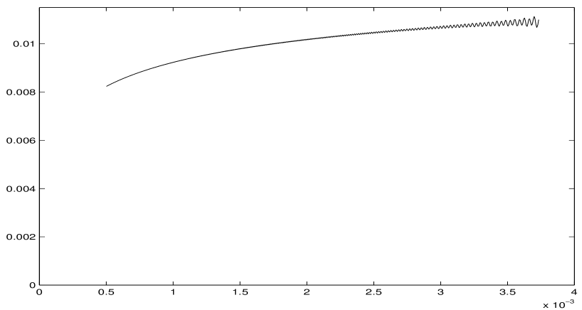
Figure 3.9: The mean squared fluctuations of the condensate $\rho$, defined as $\int^{T}(\rho(t)-\bar{\rho})^{2}dt/T$, plotted vs. $1/T$, for the same values of the parameters as in figure 3.8.

Before closing this section, I should comment a little further on the evolution of the condensate $\rho$. When $\ell=0$, fig. 3.8 shows that the oscillations are actually around zero. Because of the reduced momentum phase space, I observe that the damping of the condensate is not as efficient as in the large$-N$ $\phi^{4}$ model in $3+1$ dimension with unbroken symmetry. However, from the available data, it is not possible to decide whether the amplitude will eventually vanishes or will tend to a limiting cycle (see fig. 3.9).

On the other hand, in the case of $\ell\neq 0$, it is already clear that the condensate does not relax to the state of minimum energy compatible with the given value of $\ell$, which would correspond to the circular orbit with radius given by eq. (3.64). However, it may still relax to a circular orbit with a different radius and a different (larger) energy. More detailed and longer numerical computations are needed to decide whether the damping reduces the oscillation amplitude to zero or not.

3.4.2 Emission spectrum

Once the evolution equations for the complex mode functions has been solved, it is possible to compute the spectrum of the produced particles. First, I should say that the notion of particle number is ambiguous in a time dependent situation. Nevertheless, I may give a suitable definition with respect to some particular pointer state. I choose here two particular definitions, the same already used in the study of the $\phi^{4}$ model [85], plus a third one. The first choice corresponds to defining particles with respect to the initial Fock vacuum state, the second with respect to the instantaneous adiabatic vacuum state, and the third to the equilibrium vacuum (the true vacuum of the theory). The corresponding expressions in terms of the complex mode functions are:

$$N^{\rm in}_{k}(t)=\dfrac{1}{4}\left[\omega_{k}|z_{k}(t)|^{2}+\dfrac{|\dot{z}_{k}(t)|^{2}}{\omega_{k}}\right]-\dfrac{1}{2}$$ (3.69)

$$N^{\rm ad}_{k}(t)=\dfrac{1}{4}\left[\omega^{\rm ad}_{k}|z_{k}(t)|^{2}+\dfrac{|\dot{z}_{k}(t)|^{2}}{\omega^{\rm ad}_{k}}\right]-\dfrac{1}{2}\;,\quad\omega^{\rm ad}_{k}=\sqrt{k^{2}+m(t)^{2}}$$ (3.70)

$$N^{\rm eq}_{k}(t)=\dfrac{1}{4}\left[\omega^{\rm eq}_{k}|z_{k}(t)|^{2}+\dfrac{|\dot{z}_{k}(t)|^{2}}{\omega^{\rm eq}_{k}}\right]-\dfrac{1}{2}\;,\quad\omega^{\rm eq}_{k}=\sqrt{k^{2}+m_{\rm eq}^{2}}$$ (3.71)

I report my numerical findings on these quantities in figs. 3.10 - 3.18. Since the Lagrange multiplier tends asymptotically to a constant value $m^{2}_{\infty}$, the condensate $\rho(t)$ oscillates with frequency $m_{\infty}$ and the mode functions $z_{q}(t)$ with frequency $\omega(q)=\sqrt{q^{2}+m^{2}_{\infty}}$. This implies that particle spectra $N^{\rm in}_{k}(t)$ and $N^{\rm eq}_{k}(t)$ are more and more strongly modulated as time elapses, as figs. 3.16 and 3.17 show; on the contrary, $N^{\rm ad}_{k}(t)$ is a slowly varying function of the momentum $k$ (cfr. figs. 3.10 - 3.15), because the oscillations of the mode functions are counterbalanced by the time dependence of the adiabatic frequencies $\sqrt{k^{2}+m(t)^{2}}$. Finally, fig. 3.18 allows for a comparison of the spectra related to different initial values of the condensate.

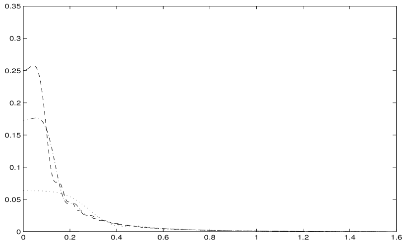
Figure 3.10: Adiabatic spectrum for $tm_{\rm eq}=0$ (solid line), $39.723$ (dotted line), $199.006$ (dashdot line) and $398.11$ (dashed line), for $\Lambda/m_{\rm eq}=20$, $\ell=0$ and $\rho_{0}=0.2$.

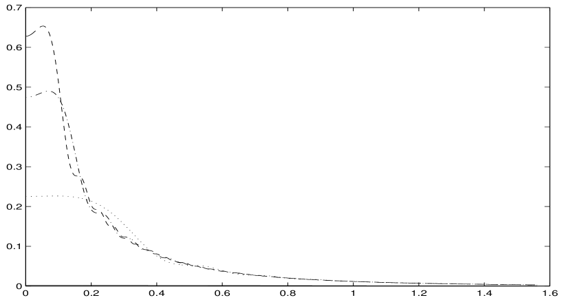
Figure 3.11: Adiabatic spectrum for $tm_{\rm eq}=0.0$ (solid line), $39.723$ (dotted line), $199.006$ (dashdot line) and $398.11$ (dashed line), for $\Lambda/m_{\rm eq}=20$, $\ell=0$ and $\rho_{0}=0.3$.

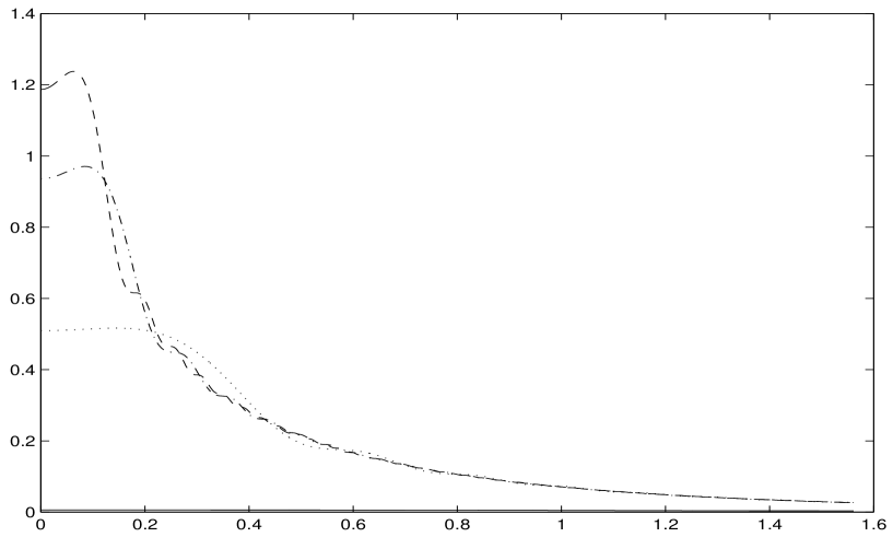
Figure 3.12: Adiabatic spectrum for $tm_{\rm eq}=0$ (solid line), $39.723$ (dotted line), $199.006$ (dashdot line) and $398.11$ (dashed line), for $\Lambda/m_{\rm eq}=20$, $\ell=0$ and $\rho_{0}=0.4$.

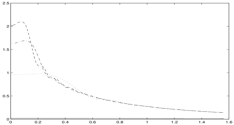
Figure 3.13: Adiabatic spectrum for $tm_{\rm eq}=0$ (solid line), $39.723$ (dotted line), $199.006$ (dashdot line) and $398.11$ (dashed line), for $\Lambda/m_{\rm eq}=20$, $\ell=0$ and $\rho_{0}=0.5$.

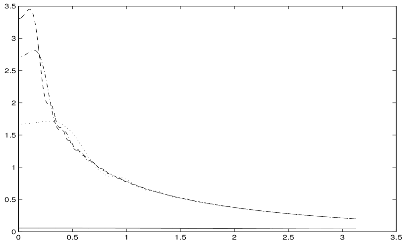
Figure 3.14: Adiabatic spectrum for $tm_{\rm eq}=0$ (solid line), $39.723$ (dotted line), $199.006$ (dashdot line) and $398.11$ (dashed line), for $\Lambda/m_{\rm eq}=20$, $\ell=0$ and $\rho_{0}=0.6$.

Figure 3.15: Adiabatic spectrum for $tm_{\rm eq}=0$ (solid line), $39.723$ (dotted line), $199.006$ (dashdot line) and $398.11$ (dashed line), for $\Lambda/m_{\rm eq}=20$, $\ell=0$ and $\rho_{0}=0.7$.

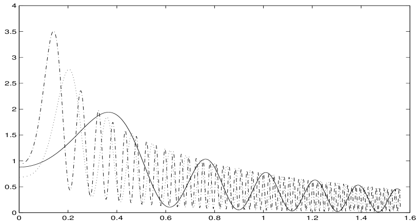
Figure 3.16: Spectrum with respect to the initial vacuum, for $tm_{\rm eq}=39.723$ (solid line), $199.006$ (dotted line) and $398.11$ (dashdot line), for $\Lambda/m_{\rm eq}=20$, $\ell=0$ and $\rho_{0}=0.5$.

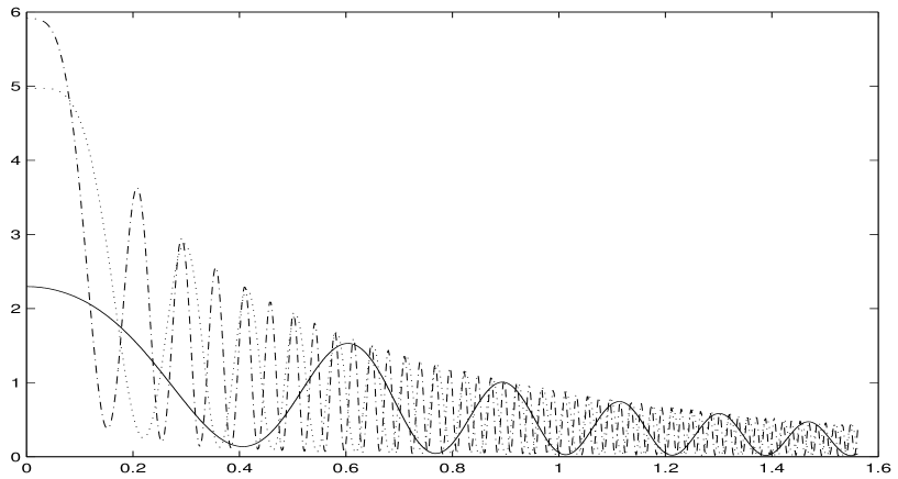
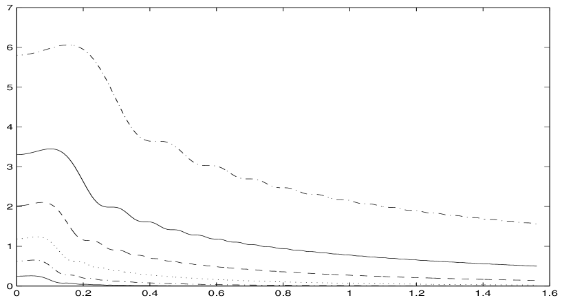
Figure 3.17: Spectrum with respect to the true vacuum, for $tm_{\rm eq}=39.723$ (solid line), $199.006$ (dotted line) and $398.11$ (dashdot line), for $\Lambda/m_{\rm eq}=20$, $\ell=0$ and $\rho_{0}=0.5$.

Figure 3.18: Adiabatic spectrum for $tm_{\rm eq}=398.11$, $\Lambda/m_{\rm eq}=20$ and $\ell=0$. The different curves correspond to different initial values for the condensate: from top to bottom, $\rho_{0}=0.7$, $0.6$, $0.5$, $0.4$, $0.3$ and $0.2$.

Looking at the momentum distribution of the created particles at different times, we see the formation of a growing peak corresponding to soft modes. I can give an analytic, self-consistent description of this behavior at large times through a perturbative approach, similar to the one used in ref. [85]. I split the time–dependent Lagrange multiplier in two parts, as in equation (3.66) and I treat the “potential” $p(t)/t$ perturbatively, as is done in [85]. I find the following solution:

$$z_{q}(t)=A_{q}e^{i\omega_{q}t}+B_{q}e^{-i\omega_{q}t}-\int_{t}^{\infty}\dfrac{\sin\omega_{q}(t^{\prime}-t)}{\omega_{q}}\dfrac{p(t^{\prime})}{t^{\prime}}z_{q}(t^{\prime})dt^{\prime}$$

which is equivalent, up to terms of order $O(1/t^{2})$, to

$$z_{q}(t) = A_{q}\left[1+\dfrac{A\sin\Psi(t)}{4im_{\infty}t}-\dfrac{A}{8\omega_{q}t}\left(\dfrac{e^{i\Psi(t)}}{\omega_{q}+m_{\infty}}+\dfrac{e^{-i\Psi(t)}}{\omega_{q}-m_{\infty}}\right)\right]e^{i\omega_{q}t}$$ (3.73)

$$+ B_{q}\left[1-\dfrac{A\sin\Psi(t)}{4im_{\infty}t}-\dfrac{A}{8\omega_{q}t}\left(\dfrac{e^{i\Psi(t)}}{\omega_{q}-m_{\infty}}+\dfrac{e^{-i\Psi(t)}}{\omega_{q}+m_{\infty}}\right)\right]e^{-i\omega_{q}t}+O\left(\dfrac{1}{t^{2}}\right)$$ (3.74)

with $\Psi(t)=2m_{\infty}t+\gamma_{1}\log t+\gamma_{2}$. The logarithmic dependence is due to the “Coulomb form” of the perturbative term $p(t)/t$ in the equations of motion. The expression (3.73) displays resonant denominators for $\omega_{q}=m_{\infty}$, that is $q=0$. The perturbative approach is valid as long as the first order correction is small compared to zeroth order. Such a condition is satisfied if

$$\dfrac{{\cal A}}{4t\,\omega_{q}(\omega_{q}-m_{\infty})}<1$$ (3.75)

that implies $q^{2}>{\cal A}/4t$ for non relativistic modes. Thus the position of the peak found before may be interpreted as the result of a weak nonlinear resonance. The asymptotic behavior of the condensate and the mode functions related to soft momenta must be obtained through non-perturbative techniques, implementing a multitime scales analysis and a dynamical resummation of sub-leading terms. A self-consistent justification of the numerical result (3.66), along with the power law relaxation behavior for the expectation value (with non-universal dynamical anomalous dimensions), are likely to be obtained following the line of the analysis performed in [85] for the $\phi^{4}$ model in $3+1$ dimensions.

From the numerical study of the complete spectrum history, I conclude that no exponentially growing (parametric or spinodal) instabilities are present in the case at hand, as apparent from Fig.s 3.10 - 3.15, which show the spectrum of produced particles with respect to the adiabatic vacuum state.

This is due to the quite different nonlinearities of the $\sigma-$model and in particular to the nonlinear constraint [see eq. (3.40)] which sets an upper bound to the quantum infrared fluctuations [see fig. 3.3]. In fact, even if the constraint disappears as the bare coupling constant $\lambda_{\rm b}$ vanishes in the infinite UV cutoff limit (asymptotic freedom), the quantum fluctuations in any given finite range of momentum remain constrained to finite values, as implied by the possibility of fully renormalize the model, including the constraint [see eq. (3.59)].

3.5 Summary and outlook

The natural continuation of this preliminary analysis is the detailed numerical study of the evolution, in order to give a precise picture of the process of dissipation via particle production in the framework of this constrained, asymptotically free model. It should be possible to determine precisely the power laws that characterize the asymptotic evolution of relevant variables, like the condensate, the Lagrange multiplier and the number of created particles. After this, one should be able to decide whether, at zero angular momentum, the damping leads to the complete dissipation of the energy stored in the condensate or the system evolves towards a limit cycle with an asymptotic amplitude different form $0$. Also a comparison with the linear model in $1+1$ dimension might be useful to understand the peculiarities of the dynamics in a constrained model.

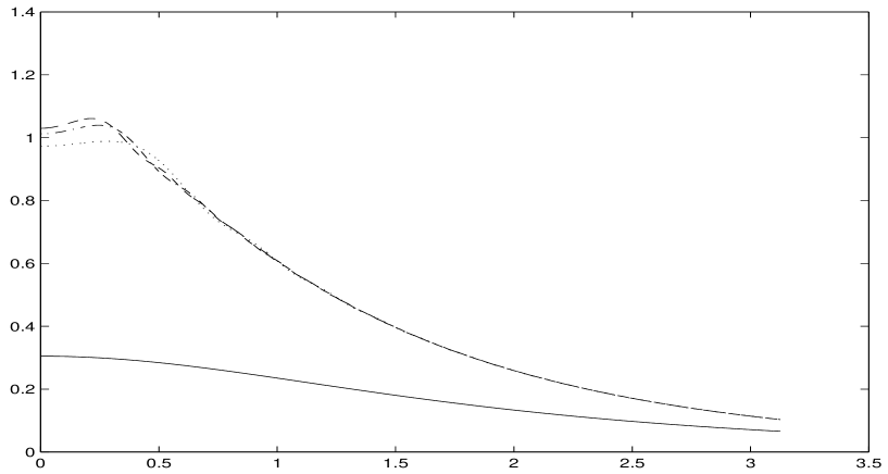
Figure 3.19: Adiabatic spectrum for $tm_{\rm eq}=0.0$ (solid line), $59.895$ (dotted line), $119.835$ (dashdot line) and $179.775$ (dashed line), for $\Lambda/m_{\rm eq}=10$, $\ell=1$ and $\rho_{0}=0.3$.

Moreover, it would be very interesting to study the dependence of the evolution on the value of $\ell$, the angular momentum of the field in the internal space. As the preliminary results presented in this paper show (see figure 3.19), the asymptotic state is far from the state of minimum energy compatible with the given value of $\ell$. Remarkably, the adiabatic spectrum of produced particles in case of $\ell\neq 0$ is broader than that one corresponding to $\ell=0$, suggesting a stronger coupling with hard modes.

Chapter 4 First steps in gauge theories

There are common relevant problems in cosmology, astrophysics and ultrarelativistic heavy ion collisions, that ask for a deeper understanding of the physics of the formation of a non–equilibrium plasma of charged particles beginning from an initial state of large energy density, its evolution, the onset of electric and magnetic screening phenomena and the generation of seeds of bulk electric and magnetic fields [108].

Taking as a first example the world of elementary particles, one of the main motivations to the use of out of equilibrium techniques comes from the possibility of studying experimentally the formation and evolution of a deconfined phase in QCD: the quark gluon plasma (QGP). It is important, for example, to understand how the quark-gluon plasma forms and equilibrates from the evolution of the parton distribution functions, to correctly compute the time scales for electromagnetic screening that cuts off small angle scattering and how a hydrodynamic picture of the space-time evolution of the plasma emerges from first principles. Also the comprehension of the possible experimental signatures of the quark gluon plasma and chiral phase transition would be very relevant. Electromagnetic probes (photons and dileptons) could provide clear signatures for an out of equilibrium chiral phase transition and the formation of quark phase transition, because they only interact electromagnetically and their mean free path is much bigger that the size of the fireball. In addition, even though these days QCD is generally accepted as the fundamental theory of strong interactions, its very rich phenomenology and its complex phase structure have not been completely unveiled yet, as recent results at finite temperature and density (color–flavor locking, color superconductivity and quark–hadron continuity) suggest [60, 109, 110, 111].

Regarding cosmology, the fascinating hypothesis of sphaleron induced B-violating processes inside the Standard Model as the basis for the baryon asymmetry, calls for a more accurate analysis of the phenomena involved.

The common ingredient in such different situations is the description of the transport properties, like the screening masses and the electrical conductivity, as well as the determination of the relaxation time scales. To this end, a much deeper understanding of collective excitations in an ultrarelativistic plasma is required: to decide if the local thermodynamical equilibrium (LTE) approximation is justified, we must compute the relaxation time scales, given by the damping rate or the lifetime of the excitations in the plasma. The quasi particle description of the collective excitations treats them as narrow resonances characterized by a Breit-Wigner distribution, whose width is related to the imaginary part of the self–energy on the mass shell. In this approximation, the damping rate turns out to be exponential.

Of course, in order to reach physically sensible results, we have to improve the models considered so far, by introducing gauge fields: a gauge invariant description of the real–time dynamics of gauge fields is required. Recently, new and unusual features of relaxation of soft degrees of freedom in gauge theories has been discovered [112]. The real time evolution of (abelian) gauge fields is very important because photoproduction is expected to be a very clear experimental signature of the chiral phase transition. It may be also relevant in the description of the creation of primordial magnetic fields in the early Universe.

In the framework of the non–equilibrium formalism the Hard Thermal Loop (HTL) resummation scheme of Braaten and Pisarsky can be rederived [112]. This is a useful scheme, which produce gauge invariant results and infrared finite transport cross sections which renders the damping rate of the excitations in the plasma [21] finite. In fact, the medium effects such as the Debye screening, the collective plasma modes and Landau damping are taken into account in the resummed Green’s functions. However, soft transverse (magnetic) photons remain unscreened and induce IR divergences. This characteristic is common to QED, QCD and scalar QED. The HTL resummation scheme may be regarded as giving a Wilsonian effective action (which turns out to be non–local) for soft modes, after the hard modes have been integrated out. Since the soft modes have in general a non perturbative dynamics leading to quite large occupation numbers, it has been hoped to get some information from the numerical simulation of the classical theory. This approach, although justified in scalar field theories, should be considered carefully when applied to gauge theories.

With the aim of understanding relaxational dynamics in the quark gluon plasma and electroweak plasma, hot scalar QED has attracted much interest [112, 113], because it has the same HTL structure as the non abelian case (for the leading term). The real time evolution of inhomogeneous expectation values with soft length scales has been considered in the weak field regime, with linearized equations which admit solutions in closed form through Laplace transform. In such a regime, the results clearly show the dominance of off-shell Landau damping processes. It is thus crucial to understand the time scales of these dissipative processes, their microscopic description and how the relaxation of soft collective excitations proceeds. The analytic structure in the $s-$plane gives the time behavior, which shows a power law tail in the relaxation of transverse field amplitudes and a logarithmic tail for longitudinal fields; this is determined by the behavior of the retarded self–energy at the Landau damping threshold. This is special of HTL at one loop and may change, should high orders be included in the computation. In this linearized regime, it is also possible to compute the Influence Functional [34], and derive an effective Langevin equation for the gauge invariant observables. Also the dissipative and noise correlation functions (kernels) and the fluctuation-dissipation relation between them, is obtained, proving in detail that a Markovian approximation fails to describe correctly the dynamics, when the processes are dominated by Landau damping.

Similar techniques have been applied to understand the non–equilibrium dynamics of a thermal plasma in a gravitational field [114, 115]. The plasma is described by a massless scalar quantum field and the matter–gravity coupling is treated semiclassically. The quantum matter back reaction on the metric is considered as a noise term in the Einstein equation, which becomes a semiclassical stochastic equation. It is equivalent to a Langevin equation, whose damping and noise kernels satisfy a definite Fluctuation–Dissipation relation.

Some results have also been obtained recently, for a condensate of arbitrary amplitude, but uniform in space. In such a situation, a Bloch-Nordsieck resummation of IR divergences, equivalent to a dynamical Renormalization Group resummation, has been applied to scalar QED, in connection with relaxation and damping in real time [116, 113]. The resummation of quasistatic transverse photons gives an anomalous logarithmic relaxation of the form $\exp(\alpha Tt\log t/t_{0})$, where $\alpha$ is related to the coupling constant and $T$ is the temperature.

The dynamical RG resummation to obtain the real time dynamics of relaxation and thermalization is equivalent to the RG resummation of divergences in Euclidean Field Theories. Here, we have the resummation of logarithmic secular terms in the perturbative solution of the evolution equation of expectation values. This analysis implies that a quasi particle description of the relaxation process is allowed only when the perturbative solution displays linear secular terms, while non–linear secular terms in lowest order signal anomalous, non–exponential relaxation.

An other important issue is the generation of an out of equilibrium plasma in scalar QED. This problem has been studied within a model containing N charged scalar fields coupled to a $U(1)$ photon, plus a neutral scalar field, which acts as an order parameter and distinguishes between the broken and unbroken symmetry phases. This model provides a convenient description of the chiral phase transition of QCD and allows the study of photon production, the electric and magnetic screening and the build up of electric conductivity. The approximation consists in considering the large $N$ limit in the scalar sector, which takes into account the non perturbative and non linear effects involved in the dynamics out of equilibrium, and the lowest order in $\alpha$, which provides a mechanism of photoproduction.

As far as the photon production is concerned, a consistent kinetic equation suitable for strongly out of equilibrium situations has been derived in [108], considering only spontaneous emission of photons (without the inclusion of stimulated processes). The exponential growth in the quantum fluctuations of the matter field, due to parametric amplification or spinodal instabilities, drives the formation of the non equilibrium quantum plasma, and a similar explosive production of photons at early times occurs, while the asymptotic distribution at late times reaches a form

$$N_{ph}(\omega)\simeq\dfrac{\alpha m^{2}}{\lambda^{2}\omega^{3}}$$ (4.1)

In case of spinodal instabilities, the asymptotic distribution diverges logarithmically with time and a resummation via the dynamical renormalization group may be in order.

The analysis of the photon production allows for an understanding of the mechanism of creation of the electromagnetic field, which shows up in correlated domains of linear size $\xi(t)\simeq\sqrt{t/m}$. The corresponding power spectrum inside the unstable band with an amplitude $\simeq\alpha/\lambda^{2}$

In [108] Magnetic and Debye screening masses are defined out of equilibrium, in order to study the dynamical aspects of electric and magnetic screening. While the magnetic mass vanishes out of equilibrium, it is possible to give a definition of a momentum and time dependent magnetic mass which has the advantage of displaying explicitly the different time scales involved in the process. The Debye mass is $\alpha m^{2}/\lambda$ for broken symmetry and is proportional to $\sqrt{t}$ for unbroken symmetry, suggesting the necessity of renormalization group resummation for the secular terms, similar to that performed in [113].

Such an analysis allows one to follow in detail the onset of the transverse electric conductivity (in the framework of the linear response theory á la Kubo) during the non equilibrium evolution and the formation of the quantum plasma. At the end of the early (linear) evolution, the long wavelength conductivity turns out to be proportional to $\alpha m/\lambda$.

A comparison with the corresponding equilibrium phenomena is very useful and shows that many results have the same dependence on the particle distribution, which is a time dependent quantity in the case of the non–equilibrium evolution, while is the static Bose–Einstein distribution in case of thermodynamic equilibrium (cfr. also [117]).

Scalar QED is very useful to clarify some phenomena which occur in an electromagnetic plasma. On the other hand, most of the non equilibrium phenomena occurring in the “ordinary” low–energy matter are described by fermionic QED. In this context, one of the older questions is how the vacuum fluctuations of the photon field affect the effective dynamics of an electron. Moreover, the program of decoherence proposes that the superselection rules coming from the conservation of charges could be induced dynamically: superposition of states with different eigenvalue of the charge operator would rapidly lose their coherence in time. This issue has been considered in [54], where the reduced density matrix for the electron has been computed in perturbation theory by means of the Feynman–Vernon influence functional technique.

An other approach is based on the extension of the HTL resummation technique to non equilibrium QFT, by means of the real time formalism in the Keldish CTP representation [118]. This extension is based on the assumption of quasi stationary distributions, which occur if the time scale of the microscopic processes in the medium is much smaller than the time scale of relaxation towards equilibrium. In this approximation, the HTL photon self energy, the resummed photon propagator and the damping rate of a hard electron in a QED plasma have the same form out of equilibrium as in equilibrium.

Regarding the study of time evolution in non abelian gauge theories, it should be noticed that some work has been done in the framework of classical Yang–Mills theory, solving the evolution equations on a lattice and modeling the two ions by means of classical wave–packets of chromoelectromagnetic field [119, 120]

Chapter 5 Conclusions

5.1 Summary

A great effort has been devoted in the last few years in order to develop a deeper qualitative and quantitative understanding of systems described by interacting quantum fields out of equilibrium. There is a class of physical problems that requires the consistent treatment of time dependent mean–fields in interaction with their own quantum or thermal fluctuations. I may mention, among others, the problem of reheating of the universe after the inflationary era of exponential growth and cooling, and the time evolution of the scalar order parameter through the chiral phase transition, soon to be probed in the heavy–ion experiments at BNL–RHIC and CERN–LHC. In these situations, a detailed description of the time–dependent dynamics is necessary to calculate the non–equilibrium properties of the system. Indeed, the development of practical general techniques and the advent of faster and cheaper computers have made possible the discovery of novel and unexpected phenomena, ranging from dissipative processes via particle production to novel aspects of symmetry breaking [55, 61, 65, 85].

From the technical point of view, it should be pointed out, first of all, that a perturbative treatment of this dynamical problem is meaningful only when the early time evolution is considered. The presence of parametric resonant bands or spinodal instabilities (in the case, respectively, of unbroken or spontaneously broken symmetries) rapidly turns the dynamics completely non–linear and non–perturbative. Thus, the asymptotic evolution at late time can be consistently studied only if approximate non–perturbative methods are applied to the problem [61].

Quite recently one of these schemes, namely the large $N$ expansion at leading order (LN) [20, 55], has been used in order to clarify some dynamical aspects of the $\phi^{4}$ theory in $3$ spatial dimensions, reaching the conclusion that the non–perturbative and non–linear evolution of the system might eventually produce the onset of a non–equilibrium Bose–Einstein condensation (BEC) of the long–wavelength Goldstone bosons usually present in the broken symmetry phase [65, 84, 85]. Another very interesting result in [84] concerns the dynamical Maxwell construction, which reproduces the flat region of the effective potential in case of broken symmetry as asymptotic fixed points of the background evolution.

In section 2.9.3 (see also ref. [80]) I have addressed the question of whether a standard BEC could actually take place as time goes on, by putting the system in a finite volume (a periodic box of size $L$) and carefully studying the volume dependence of out–of–equilibrium features in the broken symmetry phase. We summarize here the main results contained in section 2.9.3 as well as in [80]. The numerical solution shows the presence of a time scale $\tau_{L}$, proportional to the linear size $L$ of the system, at which finite volume effects start to manifest, with the remarkable consequence that the zero-mode quantum fluctuations cannot grow macroscopically large if they start with microscopic initial conditions. In fact, the size of low–lying widths at time $\tau_{L}$ is of order $L$, to be compared to order $L^{3/2}$ for the case of standard BEC. In other words we confirmed that the linear growth of the zero mode width, as found also by the authors of [65, 84, 85], really signals the onset of a novel form of dynamical BEC, quite different from the standard one described by equilibrium finite–temperature field theory. This interpretation is reinforced by the characteristics of the long–wavelength fluctuations’ spectrum.

To go beyond the gaussian approximation and study the interaction between longitudinal and transverse fluctuations, I have defined in section 2.10 an extended time dependent Hartree-Fock (tdHF) approximation for the $\phi^{4}$ QFT, which includes some non-gaussian features of the full theory (for an introduction to the standard tdHF, see ref. [18]). I have presented a rather detailed study of the dynamical evolution out of equilibrium, in finite volume (a cubic box of size $L$ in $3$D), as well as in infinite volume. For comparison, I have also analyzed some static characteristics of the theory both in unbroken and broken symmetry phases.

By means of a proper substitution of the bare coupling constant with the renormalized coupling constant (fully justified by diagrammatic consideration), I have been able to obtain equations of motion completely independent of the ultraviolet cut-off (apart from a slight dependence on inverse powers, that is, however, ineluctable because of the Landau pole). I have described in detail the shape of the ground state, showing how a broken symmetry scenario can be recovered from the quantum mechanical model, when the volume diverges.

Moreover, I have shown that, within this slightly enlarged tdHF approach that allows for non–gaussian wavefunctions, one might recover the usual gaussian HF approximation in a more controlled way. In fact, studying the late time dynamics, I have confirmed the presence of a time scale $\tau_{L}$, proportional to the linear size $L$ of the box, at which the evolution ceases to be similar to the infinite volume one. At the same time, the low–lying modes amplitudes have grown to order $L$. The same phenomenon has been observed in the $O(N)$ model [80]. Looking at this result in the framework of our extended tdHF approximation, one realizes that the growth of long–wavelength fluctuations to order $L$ in fact undermines the self–consistency of the gaussian HF itself. In fact, in our tdHF approach the initial gaussian wavefunctions are allowed to evolve into non–gaussian forms, but they simply do not do it in a macroscopic way, within a further harmonic approximation for the evolution, so that in the infinite–volume limit they are indistinguishable from gaussians at all times. But when $M^{2}$ is on average not or order $L^{0}$, but much less, as it happens for suitable initial conditions, infrared modes of order $L$ will be dominated by the quartic term in our Schroedinger equations (2.120), showing a possible internal inconsistency of the gaussians approximation.

An other manifestation of the weakness of the HF scheme is the curious “stopping at the spinodal line” of the width of the gaussian quantum fluctuations, when the initial configuration does not break the symmetry. This does not happen in the large $N$ approach because of different coupling of transverse modes (the only ones that survive in the $N\to\infty$ limit) with respect to the longitudinal modes of the $N=1$ case in the HF approach.

I have also described the non–trivial phenomenology of the infinite–volume late–time evolution in the gaussian approximation, showing how the dynamical Maxwell construction differs from the $N=\infty$ case. In fact, I have observed the presence of an unstable interval, contained in the static flat region which is forbidden as attractor of the asymptotic evolution. This region corresponds, more or less, to the spinodal region of the classical potential, with the obvious exception of the origin. In particular, I have found that the energy flux between the classical degree of freedom and the bath of quantum fluctuations is quite complex and not monotonous. In other words, since I start from initial conditions where the fluctuation energy is not minimal, there are special situations where enough energy is transferred from the bath to the condensate, pushing it beyond the top of the potential hill.

As far as the non linear $\sigma$ model in $(1+1)$D is concerned, I have shown explicitly in chapter 3 that the large $N$ limit and the large coupling limit, which turns the linear model in the non linear one, commute. I have also derived the evolution equations for the non linear model at the leading order in the $1/N$ expansion, in the case of a field condensate different from zero. I implemented the constraint by the use of a Lagrange multiplier, which I denoted $m^{2}$, since it enters the dynamics as a squared mass. I have shown that the usual renormalization procedure, which makes the bare coupling constant depend on the UV cutoff, is sufficient to get properly renormalized, that is UV finite, evolution equations. Moreover, I characterized the ground state of the model, giving an interpretation of the dynamical generation of mass (the so–called dimensional transmutation) in terms of a compromise between energetic requirements and the constraint. I then solved numerically the evolution equations and analyzed the history of the condensate and the Lagrange multiplier as well as the number of particles created during the relaxation of the condensate (the quantum fluctuations). Remarkably, I do not find any period of exponential growth for the fluctuations. Actually, no spinodal instabilities were to be expected, since the symmetry is always unbroken in $1+1$ dimensions. But there occurs also no parametric resonance, as takes place instead in the unbroken symmetry scenario of the large$-N$ $\phi^{4}$ model in $3+1$ dimensions.

The estimated dependence of the asymptotic value of the Lagrange multiplier, $m^{2}(\infty)$, on the initial condensate $\rho_{0}$, turns out to be very well approximated by an exponential, which is the exact dependence of $m^{2}(0)$ [at infinite UV cutoff, see eqs. (3.48) and (3.49)]; remarkably however, the prefactor in the exponent is changed [see eq. (3.68)]. As far as the emission of particles is concerned, we considered three different reference states: the initial state, the adiabatic vacuum state and the equilibrium vacuum state, that is the true ground state of the theory. The numerical results suggest a weak non linear resonance, yielding a relaxation of the condensate via particle production driven by power laws with non universal anomalous exponents, a result similar to what found in [85] for the asymptotic dynamics of $\phi^{4}$ in $3+1$ dimensions. Finally, since I allow the condensate to have a number $n$ of components larger than $1$, I was able to study the evolution of configurations with non–zero angular momentum $\ell$ in the internal space of the field [see eq. (3.38)]. In this case I find numerical evidence for an adiabatic spectrum broader than in the case $\ell=0$ (see figure 3.19), suggesting a stronger coupling with hard modes.

5.2 Open issues

I close this section and this work giving a list of the (in my opinion) most relevant issues still open, whose solution may result in a better understanding of both the formal and phenomenological aspects of QFT out of equilibrium:

1. The study of the Poincaré cycles in the effective hamiltonian dynamics and their dependence on the parameters [55, 80] may allow for a deeper understanding of the dynamics in finite volume.

2. The inclusion of $1/N$ corrections, which contain collisional contributions, is needed to better understand the issue of thermalization; they, in fact, may lead to a thermal asymptotic distribution and make the damping more efficient [74, 121]. With this regard, it should be stressed that finite truncations of the large–$N$ expansion introduce errors which grow with time and make the approximation unreliable on a time scale proportional to as $N^{1/2}$ [122].

3. Further study, both analytical and numerical, is needed in the generalized tdHF approach of section 2.10, to better understand the dynamical evolution of quantum fluctuations in the broken symmetry phase coupled to the condensate. An interesting direction is the investigation of the case of finite $N$, in order to interpolate smoothly the results for $N=1$ to those of the $1/N$ (at leading order) approach. It should be noted, in fact, that the theory with a single scalar field contains only the longitudinal mode (by definition), while only the transverse modes are relevant in the large $N$ limit. Hence a better understanding of the coupling between longitudinal and transverse modes is necessary. In this direction, another relevant point is whether the Goldstone theorem is respected in the HF approximation [95]. It would be interesting also to study the dynamical realization of the Goldstone paradigm, namely the asymptotic vanishing of the effective mass in the broken symmetry phases, in different models; this issue needs further study in the $2D$ case [55], where it is known that the Goldstone theorem is not valid.

4. The issue of thermalization may be addressed also by deriving a Quantum Boltzmann (kinetic) equation. The issue is relevant for the reheating problem and for the dynamics of heavy ion collisions. It would be useful a systematic quantal generalization of classical transport theory, in the presence of strong inhomogeneous mean fields, where quantum self–energy (off–shell virtual processes) are included on the same footing as collisional or real particle production processes in the plasma. To this end, the CTP generating functional may be used in order to derive an effective action principle which leads to a hierarchy of Schwinger–Dyson equations [123]. Some preliminary results [112] shows an anomalous relaxation of hard quasiparticles. Considering higher orders will include collisional processes which will give exponential decay in time. The competition between collisional and Landau damping time scales will then depend on the particular model under study.

   In any case, the approach to thermodynamic equilibrium is far from being a trivial subject. In fact, even though the time evolution of correlation functions can be described by an exact evolution (functional) equation for the corresponding generating functionals [124] (which shows many dynamical features of quantum mechanics [125]) and the classical field equations admit thermodynamic equilibrium as a fixed point, infinitely many conserved correlation functions prevent the system from approaching the fixed point, when it starts in its neighborhood. Thus, it seems that equilibrium can therefore be reached at most for suitably averaged quantities or for subsystems. A similar analysis in QFT leads to the same conclusion that a uniform approach to thermal equilibrium is prevented by the existence of infinitely many other fixed points which correspond to incoherent mixtures of eigenstates of the quantum hamiltonian [126].

   Still on this subject, it is worth noticing that an important understanding both on thermalization and on the quantal generalization of kinetic equations, has been reached recently by the authors of ref.s [127] and [128]. Using a three-loop approximation to th 2PI effective action and solving numerically the evolution equations for the two point function in $1+1$ dimensions, it is possible to show that all correlation functions approach the thermal distribution asymptotically, proving that higher loops contain indeed the collisional contributions.

5. The study of Disoriented Chiral Condensates has been started modelling the pion phenomenology with the $O(4)$ linear $\sigma$ model. It would be interesting to look for qualitative and quantitative differences in the predictions, when they are extracted from the non-linear model.

6. To better understand out of equilibrium phenomena in many areas of physics, ranging from condensed matter and statistical mechanics systems to cosmology and particle physics, it is necessary to follow the evolution of non-homogeneous condensates in several models. The derivation of the evolution equations for a spherically symmetric condensate, coupled to its quantum fluctuations, I gave in section 2.11, is a promising first step in this direction and deserves a deeper analytical and numerical analysis, in view also of its phenomenological implications. This approach may be married with the the technique developed by Aarts and Smit [129], [130], [131] and [132] in order to include the quantum fluctuations of both fermionic and bosonic fields, with inhomogeneous condensates.

7. I commented a lot in chapter 4 about the results and the open problems in non equilibrium gauge theories: they are relevant for our knowledge of phase transitions in Standard Model and baryogenesis [17, 133]. Domain walls (non homogeneous field configurations) for the non abelian gauge fields of the electroweak theory (usually known with the name of sphalerons) are thought to be responsible of the matter-antimatter asymmetry we see in our universe. Thus, in addition to the issue raised in the previous point, we need to find a dynamical scheme suitable to gauge theories. To the best of my knowledge, a non perturbative treatment in the gauge coupling is still lacking. One may try to define a mean field approximation by means of a time–dependent variational principle. It is still not clear, however, whether one should introduce the gauge conditions as constraints in the variational principle or one should enforce these conditions in the choice of the trial space [83]

   Finally, detailed computation of transport coefficients, damping rates and energy loss characteristics of the quark gluon plasma from the fundamental microtheory, QCD [38] is also needed, in view of the forthcoming experimental results from BNL and CERN.

Appendix

A Stability analysis in Quantum Mechanics

In section 2.4 I derived the classical Hamiltonians which describe the dynamics of the isotropic quantum harmonic oscillator plus a $O(N)$ invariant quartic perturbation. I used the following approximation schemes: first order in $\hbar$ and the time dependent Hartree-Fock approximation, in the case of a single degrees of freedom ($N=1$), and the leading order of the expansion in $1/N$.

In this first appendix I also describe in detail the structure of the different classical potentials, computing the position of stationary points for the three cases above. A similar computation is very useful also for the Field Theoretical models studied in chapters 2 and 3.

I will be looking for the configuration of minimum energy with respect to variation of the parameters characterizing the relevant states in each approximations. In other words I will find the variational ground states in the gaussian approximation for one loop, Hartree-Fock and Large N potentials.

A.1 $O\left(\hbar\right)$

Let us consider now the mean energy (2.37) and (2.38); I want to study the stationary points of the potential

$$v\left(\eta,a\right)=s\eta^{2}+\dfrac{\eta^{4}}{2}+\dfrac{g}{3}\left[\left(s+3\eta^{2}\right)a^{2}+\dfrac{1}{16a^{2}}\right]$$ (A-1)

as a function of two variables $\eta$ and $a$ (it is clear that the dimensionless parameter $g$, corresponding to the quantum coupling constant, must be non negative).

In the classical case, i.e. $g=0$, the dependence on the quantum width $a$ disappears, and it is enough to consider the function of the single variable $\eta$. Of course, we find the classical minima, which are $\eta=0$ when $s=1$ and $\eta=\pm 1$ when $s=-1$.

When I turn on the quantum fluctuations (i.e., $g\neq 0$), the degeneracy on the $a$ direction is removed and the positions of the stationary points is modified as follows. The gradient of the potential $v\left(\eta,a\right)$ is:

$$\begin{array}[]{ll}\dfrac{\partial v}{\partial\eta}\;=&2\eta\left(s+\eta^{2}+ga^{2}\right)\\ \dfrac{\partial v}{\partial a}\;=&\dfrac{2}{3}g\left[\left(s+3\eta^{2}\right)a-\dfrac{1}{16a^{3}}\right]\end{array}$$ (A-2)

while its Hessian matrix is:

$$H\left(\eta,a\right)=\left(\begin{array}[]{cc}2\left(s+3\eta^{2}+ga^{2}\right)&4g\eta a\\ 4g\eta a&\dfrac{2}{3}g\left[\left(s+3\eta^{2}\right)+\dfrac{3}{16a^{4}}\right]\end{array}\right)$$ (A-3)

I start from the case in which the parameter $s$ has the value $+1$; the equations (A-2) have the unique solution $\eta=0$ and $a=1/2$ and correspondingly the Hessian is diagonal with positive eigenvalues; in fact, in this case the determinant of $H$ is $h=\dfrac{g}{3}\left(4+g\right)$, the eigenvalues being $8g/3$ and $2(1+g/4)$. Thus, the stationary point found is indeed a minimum, where the potential has the value $v\left(0,1/2\right)=g/6$

On the contrary, if I consider the broken symmetry case, when $s=-1$, we see that the gradient of $v$ does not vanish for any point of the line $\eta=0$. Moreover, if I define $t=a^{2}$, I get the following equations:

$$\eta^{2}=1-gt$$ (A-4)

$$48gt^{3}-32t^{2}+1=0$$ (A-5)

A close study of the third degree polynomial leads us to the conclusion that it has two real positive roots ( $t_{1}(g)$ and $t_{2}(g)$ ) only when the parameter $g$ satisfy the constraint

$$g\leq\dfrac{16}{9}\sqrt{\dfrac{2}{3}}$$ (A-6)

As can be easily inferred by computing the value of the polynomial for $t=1/g$, the two solutions are such that

$$0<t_{1}(g)\leq\dfrac{4}{9g}\leq t_{2}(g)<\dfrac{1}{g}$$ (A-7)

The computation of the determinant of the Hessian matrix yields

$$h_{1,2}=48g^{3}\left(\dfrac{1}{g}-t_{1,2}(g)\right)\left(\dfrac{4}{9g}-t(g)_{1,2}\right)$$ (A-8)

while its trace is

$${\rm tr}H_{1,2}=4\left[1-gt_{1,2}(g)\right]+\dfrac{8}{3}g\left[2-3gt_{1,2}(g)\right]$$ (A-9)

So, I deduce that the points $\left(\pm\sqrt{1-gt_{1}(g)},\sqrt{t_{1}(g)}\right)$ are minima, while the points
$\left(\pm\sqrt{1-gt_{2}(g)},\sqrt{t_{2}(g)}\right)$ are neither maxima nor minima. The minimum values are

$$v\left(\pm\sqrt{1-gt_{1}(g)},\sqrt{t_{1}(g)}\right)=-\dfrac{1}{2}+\dfrac{4}{3}gt_{1}(g)-\dfrac{3}{2}g^{2}t_{1}(g)^{2}<0$$

In conclusion, the potential has two local minima but no global minimum, because it is not bounded from below. This means that if I choose an initial value for $a$ that is too high (or too low), I let the system to go beyond the hill near the local minima and it will not be able to come back ever again. This conclusion is in agreement with the analysis made in section 2.4.4, namely with the exponential growth of quantum fluctuations and the corresponding instability.

A.2 Hartree-Fock

If I now consider the formula for the Energy in the Hartree-Fock approximation, eq. (2.51), the potential turns out to be:

$$v\left(\eta,a\right)=s\eta^{2}+\dfrac{\eta^{4}}{2}+\dfrac{g}{3}\left[\left(s+3\eta^{2}\right)a^{2}+\dfrac{1}{16a^{2}}+\dfrac{g}{2}a^{4}\right]$$ (A-10)

This computation is equivalent to the search for the ground state by a variational principle, using the gaussian packet (2.22) as a trial state and then minimizing with respect to its parameters $\sigma$ and $X$.

The classical approximation ($g=0$) is, as before, quite trivial.

When $g\neq 0$, the first partial derivatives (the gradient) of the function $v\left(\eta,a\right)$ are:

$$\begin{array}[]{ll}\dfrac{\partial v}{\partial\eta}\;=&2\eta\left(s+\eta^{2}+ga^{2}\right)\\ \dfrac{\partial v}{\partial a}\;=&\dfrac{2}{3}g\left[\left(s+3\eta^{2}\right)a-\dfrac{1}{16a^{3}}+ga^{3}\right]\end{array}$$ (A-11)

while the Hessian matrix is

$$H\left(\eta,a\right)=\left(\begin{array}[]{cc}2\left(s+3\eta^{2}+ga^{2}\right)&4g\eta a\\ 4g\eta a&\dfrac{2}{3}g\left(s+3\eta^{2}+\dfrac{3}{16a^{4}}+3ga^{2}\right)\end{array}\right)$$ (A-12)

If the parameter $s$ takes the value $+1$ the system (A-11) has only one solution: $(\eta=0,a=\sqrt{T(g)})$, where $T(g)$ is the unique positive real root of the polynomial

$$16gt^{3}+16t^{2}-1$$ (A-13)

Corresponding to this solution the Hessian matrix is diagonal with positive eigenvalues; in fact, the determinant of $H$ takes the value $h={\textstyle{8\over 3}}g\left[1+gT(g)\right]\left[2+3gT(g)\right]$, the two eigenvalues being $2[1+gT(g)]$ and $4g[2+3gT(g)]/3$. The stationary point found is actually a minimum, whose value is

$$v(0,\sqrt{T(g)})=\dfrac{2}{3}gT(g)\left(1+\dfrac{3}{4}gT(g)\right)$$

The most interesting case is instead when the parameter $s$ takes the value $s=-1$: a solution is $(\eta=0,a=\sqrt{\tau(g)})$, where $\tau(g)$ is the only (positive) real root of the polynomial:

$$16gt^{3}-16t^{2}-1$$ (A-14)

The Hessian matrix corresponding to this solution is diagonal again and it has positive eigenvalues; in fact, the determinant is $h={\textstyle{8\over 3}}g\left[g\tau(g)-1\right]\left[3g\tau(g)-2\right]$. Note that $\tau(g)>1/g$. Thus, the stationary point is a minimum, whose value is

$$v(0,\sqrt{\tau(g)})=-\dfrac{2}{3}g\tau(g)\left(1-\dfrac{3}{4}g\tau(g)\right)$$ (A-15)

which is positive for $g>16/3\sqrt{3}$. There are also two more solutions, solving the equations

$$\eta^{2}=1-gt$$ (A-16)

$$32gt^{3}-32t^{2}+1=0$$ (A-17)

where I define $t=a^{2}$. The third degree polynomial has two real positive solutions ($t_{1}(g)$ and $t_{2}(g)$) only when

$$g\leq\dfrac{8}{3}\sqrt{\dfrac{2}{3}}$$ (A-18)

($t_{1}(g)$ and $t_{2}(g)$) satisfy the relation

$$0<t_{1}(g)\leq\dfrac{2}{3g}\leq t_{2}(g)\leq\dfrac{1}{g}<\tau(g)$$ (A-19)

For these values of $g$, the “symmetric minimum” (A-15) is negative. The computation of the determinant of the Hessian matrix yields the result:

$$h=32g^{3}\left(\dfrac{1}{g}-t_{1,2}\right)\left(\dfrac{2}{3g}-t_{1,2}\right)$$ (A-20)

while the trace is:

$${\rm tr}H=4\left[1-gt_{1,2}(g)\right]+\dfrac{4}{3}g\left[4-3gt_{1,2}(g)\right]$$ (A-21)

from which I realize that the stationary points $\left(\pm\sqrt{1-gt_{1}(g)},\sqrt{t_{1}(g)}\right)$ are minima, while the stationary points $\left(\pm\sqrt{1-gt_{2}(g)},\sqrt{t_{2}(g)}\right)$ are not minima neither maxima. The value of the two minima is:

$$v\left(\pm\sqrt{1-gt_{1}(g)},\sqrt{t_{1}(g)}\right)=-\dfrac{1}{2}+\dfrac{4}{3}gt_{1}(g)-g^{2}t_{1}(g)^{2}$$ (A-22)

that is always negative for any value of $g$. Comparing the two expressions (A-15) and (A-22), it is possible to decide which one is the global minimum.

In conclusion, the stability properties of the HF potential are completely different from those I had in the previous section: thanks to the Hartree–Fock self–consistent term, the potential has now at least one global minimum. This prevents the fluctuations from growing exponentially for later times.

A.3 Large $N$

I repeat here the analysis of the potential $v\left(\eta,a\right)$ for the model with $O\left(N\right)$ symmetry; now, the function is [cfr. (2.72)]:

$$v\left(\eta,a\right)=s\eta^{2}+\dfrac{\eta^{4}}{2}+\dfrac{g}{3}\left[\left(s+\eta^{2}\right)a^{2}+\dfrac{g}{6}a^{4}+\dfrac{1}{16a^{2}}\right]$$ (A-23)

Again, the computation corresponds to the search for the best approximation to the ground state by means of a variational principle in which I use the gaussian packet

$$\left\langle\vec{x}\right|\left.\Psi\right\rangle=\dfrac{1}{(2\pi\sigma)^{N/4}}\exp\left[-\sum_{i=1}^{N-1}\dfrac{x_{i}^{2}}{4\sigma}\right]\exp\left[-\dfrac{(x_{N}-\sqrt{N}X)^{2}}{4\sigma}\right]$$ (A-24)

as a trial state and I minimize with respect to $\sigma$ e $X$.

For $g\neq 0$ we get the following structure. The gradient is

$$\begin{array}[]{ll}\dfrac{\partial v}{\partial\eta}\;=&2\eta\left(s+\eta^{2}+\dfrac{g}{3}a^{2}\right)\\ \dfrac{\partial v}{\partial a}\;=&\dfrac{2}{3}g\left[\left(s+\eta^{2}\right)a-\dfrac{1}{16a^{3}}+\dfrac{g}{3}a^{3}\right]\end{array}$$ (A-25)

while the Hessian matrix is now

$$H\left(\eta,a\right)=\left(\begin{array}[]{cc}2\left(s+3\eta^{2}+\dfrac{g}{3}a^{2}\right)&\dfrac{4}{3}g\eta a\\ \dfrac{4}{3}g\eta a&\dfrac{2}{3}g\left(s+\eta^{2}+\dfrac{3}{16a^{4}}+ga^{2}\right)\end{array}\right)$$ (A-26)

If the parameter $s$ is $+1$, the system made by the equations (A-25) has the following unique solution: $(\eta=0,a=\sqrt{T(g)})$, where $T(g)$ is the only real positive root of the polynomial

$$16gt^{3}+48t^{2}-3$$ (A-27)

Corresponding to this solution, the Hessian matrix has positive eigenvalues; in fact, the determinant of $H$ takes the value $h={\textstyle{8\over 3}}g\left[1+{\textstyle{g\over 3}}T(g)\right]\left[2+gT(g)\right]$. Thus, the stationary point found is a minimum, whose value is

$$v(0,\sqrt{T(g)})=\dfrac{2}{3}gT(g)\left[1+\dfrac{g}{4}T(g)\right]$$

The couple $\left(\eta=0,a=\sqrt{\tau(g)}\right)$ is the unique solution, in the case of $s=-1$, where $\tau(g)$ is the real positive root of the polynomial

$$16gt^{3}-48t^{2}-3$$ (A-28)

An expansion of the solution $\tau(g)$ in power series of $g$ yields:

$$\tau(g)=\dfrac{3}{g}+\dfrac{g}{2^{4}3}+\dfrac{g^{3}}{2^{7}3^{3}}+O(g^{5})$$

The Hessian matrix is diagonal and its eigenvalues are both positive, the determinant being $h={\textstyle{8\over 3}}g\left[{\textstyle{g\over 3}}\tau(g)-1\right]\left[\tau(g)-2\right]$, thanks to the fact that $\tau(g)>3/g$; then, the stationary point is a minimum again, whose value is

$$v(0,\sqrt{\tau(g)})=-\dfrac{2}{3}g\tau(g)\left[1-\dfrac{g}{4}\tau(g)\right]\approx-\dfrac{1}{2}+\dfrac{g^{2}}{2^{4}3^{2}}+\dfrac{7}{2^{9}3^{4}}+O(g^{6})$$

In the classical limit ($g\rightarrow 0$) this minimum is at infinity and it has the same value as the ones which belong to the lines $\eta=\pm 1$.

A definition of the effective potential in Quantum Mechanics

Since I use a similar procedure in the QFT model I study in chapter 2, it is interesting to see how one can define the effective potential in the simpler setting of quantum mechanics.

In section 2.9.1 I define the effective potential as the minimum of the potential energy ${\cal V}$ at fixed field condensate $\bar{\boldsymbol{\phi}}$. Let us now apply this definition to the expression (A-23) for the classical potential. I first of all specify one value for $\eta$. Then I minimize the energy with respect to the quantum width $a$, keeping the value of $\eta$ fixed, which is done by solving the stationary condition

$$48gt^{3}+48(s+\eta^{2})t^{2}-3=0$$ (A-29)

where $t$ is defined as $a^{2}$, and $\eta$ appears as a parameter. This cubic equation may be considered as the counterpart of the field–theoretical gap equation [cfr. (2.9.1)], in this quanto–mechanical case. Substituting the solution $t(\eta)$ of (A-29) in the function of two variables $v\left(\eta,a\right)$ turns it in a different function of the single variable $\eta$, which is the effective potential $v_{\rm eff}(\eta)$:

$$v_{\rm eff}(\eta)=\left(s+\dfrac{2g}{3}t(\eta)\right)\eta^{2}+\dfrac{\eta^{4}}{2}+\dfrac{2g}{3}st(\eta)+\dfrac{g^{2}}{6}t(\eta)^{2}$$ (A-30)

of the $O(N)$ quartic harmonic oscillator in the large $N$ limit.

A.4 Numerical Computation for $g=0.1$

I present here some numerical result in the case the dimensionless coupling constant has the value $g=0.1$.

• The solutions of the equation (A-5) are $t_{1}=0.1792016$ and $t_{2}=6.6619726$; the minima correspond to $(\eta=\pm 0.9909994,a=0.4233221)$, where the value of the potential is $-0.4765882$.

• The solution of the equation (A-13) is $0.2469689$ and corresponds to $(\eta=0,a=0.4969597)$, where the potential takes the value $0.0167696$.

• In the case (A-14), the root of the polynomial is $10.006242$, corresponding to the stationary point $(\eta=0,a=3.1632645)$ and to the potential value $v=-0.1664584$.

• The equation (A-17) has the solution $t=0.1783747$; the two minima are $(\pm 0.9910411,0.4223443)$ and the potential is $-0.4764288$.

• The equation (A-27) has only one positive real solution, whose value is $0.2489690$, the corresponding minimum is $(\eta=0,a=0.4989680)$ where the potential takes the value $0.0167012$.

• Finally, the solution of the equation (A-28) is $30.002083$ corresponding to the stationary point $(\eta=0,a=5.4774157)$ and to the minimum $v=-0.4999306$.

I can summarize the results in the following table:

$$\begin{array}[]{|c|c|c|c|}\hline\cr case&eq.n.&solutions&v(\eta,a)\\ \hline\cr 1L/s=+1&&(0,1/2)&0.0166667\\ \hline\cr 1L/s=-1&\ref{pol1}&(\pm 0.9909994,0.4233221)&-0.4765882\\ \hline\cr HF/s=+1&\ref{pol2}&(0,0.4969597)&0.0167696\\ \hline\cr HF/s=-1&\ref{pol3}&(0,3.1632645)&-0.1664584\\ &\ref{pol4}&(\pm 0.9910411,0.4223443)&-0.4764288\\ \hline\cr N=\infty/s=+1&\ref{pol5}&(0,0.4989680)&0.0167012\\ \hline\cr N=\infty/s=-1&\ref{pol6}&(0,5.4774157)&-0.4999306\\ \hline\cr\end{array}$$

B Details of the numerical analysis

I present here the precise form of the evolution equations for the field background and the quantum mode widths, which control the out–of–equilibrium dynamics of the $\phi^{4}$ model in finite volume at the leading order in the $1/N$ approach, as described in section 2.9.2, and in the time dependent Hartree–Fock approach of section 2.10.3.

Actually, for understanding the structure of the equations, the quanto–mechanical case of section 2.4 is enough. Eqs. (2.48) and (2.68) may be written as

$$\left[\dfrac{d^{2}}{dt^{2}}+\left(\omega^{2}-2\eta^{2}\right)\right]\eta=0\;,\quad\left[\dfrac{d^{2}}{dt^{2}}+\omega^{2}\right]a-\dfrac{1}{16a^{3}}=0$$ (B-1)

where $\omega^{2}=s+3\eta^{2}+ga^{2}$, or

$$\left[\dfrac{d^{2}}{dt^{2}}+\omega^{2}\right]\eta=0\;,\quad\left[\dfrac{d^{2}}{dt^{2}}+\omega^{2}\right]a-\dfrac{1}{16a^{3}}=0$$ (B-2)

where $\omega^{2}=s+\eta^{2}+ga^{2}$.

The field theoretical is quantitatively more complicated, as each mode corresponds to a different equation and all equations are mean field coupled; nevertheless, it is conceptually very similar.

I come immediately to it and I restrict here my attention to the tridimensional case. Let us begin by noticing that each eigenvalue of the Laplacian operator in a $3D$ finite volume is of the form $k_{n}^{2}=\left({\textstyle{2\pi\over L}}\right)^{2}n$, where $n$ is a non–negative integer obtained as the sum of three squared integers, $n=n_{x}^{2}+n_{y}^{2}+n_{z}^{2}$. Then we associate a degeneracy factor $g_{n}$ to each eigenvalue, representing the number of different ordered triples $(n_{x},n_{y},n_{z})$ yielding the same $n$. One may verify that $g_{n}$ takes on the continuum value of $4\pi k^{2}$ in the infinite volume limit, where $k=\left({\textstyle{2\pi\over L}}\right)^{2}n$ is kept fixed when $L\to\infty$.

Now, the system of coupled ordinary differential equations is, in case of the large $N$ approach,

$$\left[\dfrac{d^{2}}{dt^{2}}+M^{2}\right]\phi=0\;,\quad\left[\dfrac{d^{2}}{dt^{2}}+\left(\dfrac{2\pi}{L}\right)^{2}n+M^{2}\right]\sigma_{n}-\dfrac{1}{4\sigma_{n}^{3}}=0$$ (B-3)

while I have

$$\left[\dfrac{d^{2}}{dt^{2}}+\left(M^{2}-2\lambda\phi^{2}\right)\right]\phi=0\;,\quad\left[\dfrac{d^{2}}{dt^{2}}+k_{n}^{2}+M^{2}\right]\sigma_{n}-\dfrac{1}{4\sigma_{n}^{3}}=0$$ (B-4)

for the time dependent Hartree-Fock approach [cfr eq. (2.166)]. Here the index $n$ ranges from $0$ to ${\cal N}^{2}$, ${\cal N}=\Lambda L/2\pi$ and $M^{2}(t)$ is defined by the eq. (2.110) in case of unbroken symmetry and by eq. (2.111) in case of broken symmetry for the large $N$ approach, while the suitable definitions are eqs. (2.167) and (2.168). The back–reaction $\Sigma$ reads, in the notations of this appendix

$$\Sigma=\dfrac{1}{L^{D}}\sum_{n=0}^{{\cal N}^{2}}g_{n}\sigma_{n}^{2}$$ (B-5)

Technically it is simpler to treat an equivalent set of equations, which are formally linear and do not contain the singular Heisenberg term $\propto\sigma_{n}^{-3}$. This is done by introducing the complex mode amplitudes $z_{n}=\sigma_{n}\exp(i\theta_{n})$, where the phases $\theta_{n}$ satisfy $\sigma_{n}^{2}\dot{\theta}_{n}=1$. Then I find a discrete version of the equations studied for instance in ref. [61],

$$\left[\dfrac{d^{2}}{dt^{2}}+\left(\dfrac{2\pi}{L}\right)^{2}n+M^{2}\right]z_{n}=0\;,\quad\Sigma=\dfrac{1}{L^{D}}\sum_{n=0}^{{\cal N}^{2}}g_{n}|z_{n}|^{2}$$ (B-6)

subject to the Wronskian condition

$$z_{n}\,\dot{\bar{z_{n}}}-\bar{z_{n}}\,\dot{z}_{n}=-i$$ (B-7)

One realizes that the Heisenberg term in $\sigma_{n}$ corresponds to the centrifugal potential for the motion in the complex plane of $z_{n}$. Looking at the figs. 2.13 or 2.20, we can see that the motions of the quantum modes correspond qualitatively to orbits with very large eccentricities. In fact, there are instants in which $\sigma_{n}$ is very little and the angular velocity $\dot{\theta}_{n}$ is very large. This is the technical reason for preferring the equations in the form (B-6).

Let us now come back to the equations (B-6). To solve these evolution equations, I have to choose suitable initial conditions respecting the Wronskian condition. In case of unbroken symmetry, once I have fixed the value of $\phi$ and its first time derivative at initial time, the most natural way of fixing the initial conditions for the $z_{n}$ is to require that they minimize the energy at $t=0$. I can obviously fix the arbitrary phase in such a way to have a real initial value for the complex mode functions

$$z_{n}(0)=\dfrac{1}{\sqrt{2\Omega_{n}}}\hskip 28.45274pt\dfrac{dz_{n}}{dt}(0)=\imath\sqrt{\dfrac{\Omega_{n}}{2}}$$ (B-8)

where $\Omega_{n}=\sqrt{k^{2}_{n}+M^{2}(0)}$. The initial squared effective mass $M^{2}(t=0)$, has to be determined self-consistently, by means of its definition (2.110) or (2.167).

In case of broken symmetry, the gap equation, (2.111) or (2.168), is a viable mean for fixing the initial conditions only when $\phi$ lies outside the spinodal region [cfr. eq (2.115) or (2.174)]; otherwise, the gap equation does not admit a positive solution for the squared effective mass. In that case, I have to resort to other methods, in order to choose the initial conditions. Following the discussion presented in 2.9.2, one possible choice is to set $\sigma_{k}^{2}={\textstyle{1\over 2\sqrt{k^{2}+|M^{2}|}}}$ for $k^{2}<|M^{2}|$ and then solve the corresponding gap equation (2.114). An other acceptable choice would be to solve the gap equation (2.114), once I have set a massless spectrum for all the spinodal modes but the zero mode, which is started from an arbitrary, albeit microscopic, value.

There is actually a third possibility, that is in some sense half a way between the unbroken and broken symmetry case. I could allow for a time dependent bare mass, in such a way to simulate a sort of cooling down of the system. In order to do that, I could start with a unbroken symmetry bare potential (which fixes initial conditions naturally via the gap equation) and then turn to a broken symmetry one after a short interval of time. This evolution is achieved by a proper interpolation in time of the two inequivalent parameterizations of the bare mass, eqs. (2.91) and (2.98) for large $N$ or (2.137) and (2.147) for Hartree–Fock.

In case of large $N$, I looked for the influence this different choices could produce in the results and indeed they depend very little and only quantitatively from the choice of initial condition I make. As far as the Hartree–Fock approximation is concerned, I commented extensively in section 2.10.5 the consequences of choosing different gap equations to fix the initial conditions for the quantum fluctuations.

Finally, I used a $4$th order Runge-Kutta algorithm to solve the coupled differential equations (B-6), performing the computations in boxes of linear size ranging from $L=20\pi$ to $L=400\pi$ and verifying the conservation of the Wronskian to order $10^{-5}$. Typically, I have chosen values of $\cal N$ corresponding to the UV cutoff $\Lambda$ equal to small multiples of $m$ for unbroken symmetry and of $v\sqrt{\lambda}$ for broken symmetry. In fact, the dynamics is very weakly sensitive to the presence of the ultraviolet modes, once the proper subtractions are performed. This is because only the modes inside the unstable (forbidden or spinodal) band grow exponentially fast, reaching soon non perturbative amplitudes (i.e. $\approx\lambda^{-1/2}$), while the modes lying outside the unstable band remains perturbative, contributing very little to the quantum back–reaction [85] and weakly affecting the overall dynamics. The unique precaution to take is that the initial conditions be such that the unstable band lay well within the cutoff. As a final comment, I want to stress that also in the case of the non linear $\sigma$ model in $(1+1)$D, the dynamics is insensitive to the addition of ultraviolet modes, once the proper renormalization is performed. Most important, this happens even in the absence of parametric instabilities because the theory is asymptotically free.

C Gap Equations from tdHF for $N>1$

As we have seen, it is generally accepted that, in order to study the in medium properties of systems at finite density and temperature, the trivial perturbative approach is not well suited. When dealing with field theory at finite temperature, some sort of resummation is needed and a mean field approach has been much used in the past.

As an example, the $\sigma$ meson and pions’ masses have been studied in the framework of the $O(N)$ symmetric linear $\sigma$ model [95], using the Cornwall-Jackiw-Tomboulis (CJT) formalism and in the Hartree–Fock approximation. The CJT effective action for composite operators is a functional of the expectation value of the field and of the quantum propagator

$$\Gamma(\phi_{c}(x),G(x,y))$$ (C-1)

and is the generating functional of the two particle irreducible vacuum graphs.

The stationary condition for the effective potential yields the usual Schwinger–Dyson equations which reduce, in the HF scheme, to gap equations for the in–medium dressed masses. In ref. [95] the gap equations for finite $N$ and in the large $N$ limit are derived and a renormalization attempted both in the cutoff and counterterm schemes. The renormalization procedures consistent with the chiral limit and a finite value for the UV cutoff turns out to be possible only in large $N$. In other words, the Nambu–Goldstone’s theorem would not be satisfied at finite temperature. This is because if one performs the renormalization after a non–perturbative partial resummation, renormalization constants may acquire some dependence on the medium properties. Also the in–medium modifications of meson properties, like their mass and decay width, are studied, computing the contribution to meson self–energy of the setting sun diagram with internal dressed (HF) propagators.

It is interesting to compare this approach with others based on a different definition of masses, or implementing different resummation. For example, recently [134] it has been shown that the Nambu–Goldstone’s theorem is safe, provided one defines the masses as the curvature of the effective potential in the CJT formalism and in the Hartree–Fock approximation. In this case, the renormalization is performed by an extension of the auxiliary field method and some conclusions about how the order of the chiral phase transition depends on the inclusion of the quantum and thermal fluctuations are reached. Other resummation schemes have been proposed, which guarantee that the Goldstone’s theorem is satisfied. One of them is the large–$N$ limit. Another one, the 2PPI expansion, was introduced to study the the $O(N)$ linear $\sigma$ model at finite temperature [135], and has the merit of summing the seagull and bubble graphs to all orders, going beyond the gaussian Hartree approximation.

In this appendix, I am interested in showing how to derive the gap equations in the gaussian approximation for the longitudinal ($\sigma$ meson) and transverse (pions) modes, starting from eqs. (2.123), (2.124) and (2.125). I will also make some comments one the difficulties one finds when a renormalization is attempted.

Eq. (2.124) may be written also as

$$(\omega_{k}^{2})_{ij}=(k^{2}+m_{b}^{2})\delta_{ij}+\lambda_{b}\left[\mathrm{Tr}(\Sigma)\delta_{ij}+2\Sigma_{ij}\right]$$ (C-2)

with $\Sigma$ defined as

$$\Sigma^{ij}=\dfrac{1}{L^{D}}\sum_{k^{\prime}\neq\pm k}\langle\varphi^{i}_{k^{\prime}}\varphi^{j}_{k^{\prime}}\rangle$$ (C-3)

The total energy, divided in the kinetic and potential parts, reads

$$\mathcal{E}=\mathcal{T}(\dot{\boldsymbol{\phi}},(\dot{\sigma}_{k}^{2})_{ij})+\mathcal{V}(\boldsymbol{\phi},(\sigma_{k}^{2})_{ij})$$ (C-4)

where the $(\sigma_{k})_{ij}$ are the widths of the gaussian wavefunctional and $\boldsymbol{\phi}$ is the field condensate. The potential $\mathcal{V}$ [cfr. eq. (2.87) for large $N$] may be written in compact form

$$\mathcal{V}=\dfrac{1}{2L^{D}}\mathrm{Tr}\sum_{k}\left[(k^{2}+m_{b}^{2})(\sigma_{k}^{2})+\dfrac{1}{4}(\sigma_{k}^{2})^{-1}\right]-\dfrac{\lambda_{b}}{2}(\boldsymbol{\phi}^{2})^{2}+\dfrac{1}{2}m_{b}^{2}\boldsymbol{\phi}^{2}$$ (C-5)

$$+\dfrac{\lambda_{b}}{4}(\mathrm{Tr}\Sigma)^{2}+\dfrac{\lambda_{b}}{2}\mathrm{Tr}(\Sigma^{2})$$

I now distinguish the longitudinal width $\sigma_{kL}^{2}$ from the transverse one $\sigma_{kT}^{2}$ and write

$$(\mathrm{Tr}\Sigma)^{2} = (\boldsymbol{\phi}^{2}+\Sigma_{L}+(N-1)\Sigma_{T})^{2}$$ (C-6)

$$\mathrm{Tr}(\Sigma^{2}) = (\boldsymbol{\phi}^{2}+\Sigma_{L})^{2}+(N-1)\Sigma_{T}^{2}$$ (C-7)

where

$$\Sigma_{L}=\dfrac{1}{L^{D}}\sum_{k}\sigma_{kL}^{2}\qquad\Sigma_{T}=\dfrac{1}{L^{D}}\sum_{k}\sigma_{kT}^{2}$$ (C-8)

If I now fix the value of the condensate and try to minimize w.r. to the quantum fluctuations, I get the two coupled bare gap equations:

$$M_{L}^{2}=m_{b}^{2}+\lambda_{b}\left[3\boldsymbol{\phi}^{2}+\dfrac{1}{L^{D}}\left(3\sum_{k}\dfrac{1}{2\sqrt{k^{2}+M_{kL}^{2}}}+(N-1)\sum_{k}\dfrac{1}{2\sqrt{k^{2}+M_{kT}^{2}}}\right)\right]$$ (C-9)

$$M_{T}^{2}=m_{b}^{2}+\lambda_{b}\left[\boldsymbol{\phi}^{2}+\dfrac{1}{L^{D}}\left(\sum_{k}\dfrac{1}{2\sqrt{k^{2}+M_{kL}^{2}}}+(N+1)\sum_{k}\dfrac{1}{2\sqrt{k^{2}+M_{kT}^{2}}}\right)\right]$$ (C-10)

In the infinite volume limit, these two gap equations can be written in terms of the divergent momentum integral defined in (2.91):

$$M_{L}^{2} = m_{b}^{2}+3\lambda_{b}\boldsymbol{\phi}^{2}+3\lambda_{b}I_{D}(M_{L}^{2},\Lambda)+\lambda_{b}(N-1)I_{D}(M_{T}^{2},\Lambda)$$ (C-11)

$$M_{T}^{2} = m_{b}^{2}+\lambda_{b}\boldsymbol{\phi}^{2}+\lambda_{b}I_{D}(M_{L}^{2},\Lambda)+\lambda_{b}(N+1)I_{D}(M_{T}^{2},\Lambda)$$

If we consider a quantum state, which is spherically symmetric in the internal state, $\boldsymbol{\phi}=0$ and $M_{L}^{2}=M_{T}^{2}$. This allows for a definition of the equilibrium, renormalized mass $m$ and a parametrization of the bare mass, which reads

$$m_{b}^{2}=m^{2}-(N+2)\lambda_{b}I_{D}(m^{2},\Lambda)$$ (C-12)

The gap equations become

$$M_{L}^{2}=m^{2}+3\lambda_{b}\boldsymbol{\phi}^{2} + 3\lambda_{b}[I_{D}(M_{L}^{2},\Lambda)-I_{D}(m^{2},\Lambda)]$$ (C-13)

$$+ \lambda_{b}(N-1)[I_{D}(M_{T}^{2},\Lambda)-I_{D}(m^{2},\Lambda)]$$

$$M_{T}^{2}=m^{2}+\lambda_{b}\boldsymbol{\phi}^{2} + \lambda_{b}[I_{D}(M_{L}^{2},\Lambda)-I_{D}(m^{2},\Lambda)]$$ (C-14)

$$+ \lambda_{b}(N+1)[I_{D}(M_{T}^{2},\Lambda)-I_{D}(m^{2},\Lambda)]$$

The renormalization of the coupling constant is still to be performed. If I trivially generalize to $N>1$ the $N=1$ one–loop resummed perturbative relation between the bare and running coupling constant, I get

$$\lambda(\mu)=\dfrac{\lambda_{\rm b}(\Lambda)}{1-(N+2)\dfrac{\lambda_{\rm b}(\Lambda)}{8\pi^{2}}\ln\dfrac{\Lambda}{\mu}}$$ (C-15)

Now, the gap equations can be solved, but the two squared masses retain a logarithmic dependence on the UV cutoff (plus the usual inverse power corrections, always present due to the the Landau pole). Notice that, for $N>1$, this is not the solution of the renormalization group flow, which is given replacing the $N+2$ coefficient in the denominator with $(N+8)/3$ [136]. In any case, it is not possible to make the logarithmic dependence disappear. In addition, if I consider guassian wavefunctional with mean value different from zero, their energy w.r. to the ground state is not UV finite, as happened for the $N=1$ case of section 2.10.1; thus a substitution similar to (2.10) is necessary.

These unpleasant features signal that the tdHF defined in section 2.10 is not completely renormalizable, (at least in the gaussian approximation), as, on the contrary, is the full theory. Something crucial for the renormalizability is lost when one reduces himself to this approximation scheme. In order to have finite renormalized masses and energy differences, I need to implement a more sophisticated resummation than the simple one–loop relation (C-15). An enlightening view on the procedure to follow is contained in ref. [134], where a counterterm renormalization scheme is used. Along this line, finite renormalized gap equations can be obtained [137]. In any case, a diagrammatic explanation of the resummation needed is far from being clear.

D Evolution of a spherically symmetric condensate in $2+1$ dimensions

I consider here a derivation similar to that of section 2.11 in $(2+1)$D. Recalling that the laplacian in spherical coordinates reads in this case,

$$\nabla^{2}F=\dfrac{1}{r}{d\over dr}\left(r{dF\over dr}\right)+\dfrac{1}{r^{2}}\dfrac{d^{2}F}{d\theta^{2}}$$ (D-1)

and, defining the radial [$u(r)$] and angular [${\cal T}(\theta)$] functions as $F=u/\sqrt{r}{\cal T}$, I obtain the following equations for the functional basis:

$$\begin{array}[]{ll}&\dfrac{d^{2}{\cal T}_{\nu}}{d\theta^{2}}+\nu^{2}{\cal T}_{\nu}=0\\ \\ &\dfrac{d^{2}u_{\nu}}{dr^{2}}-\dfrac{\nu^{2}-1/4}{r^{2}}\,u_{\nu}=0\end{array}$$ (D-2)

which have the following solutions:

$$F_{\nu}(r,\theta)=(A_{\nu}\,r^{\nu}+B_{\nu}\,r^{-\nu})\,\exp(i\,\nu\,\theta)$$ (D-3)

Spherical symmetry
in case of rotational invariance, we have

$$\phi(x)=\dfrac{\varphi(r)}{\sqrt{2\pi\,r}}\;,\quad\pi(x)=\dfrac{p(r)}{\sqrt{2\pi\,r}}$$ (D-4)

and we can expand the 2-point functions as follows
($rr^{\prime}\cos\theta=x\cdot x^{\prime}$):

$$\Gamma(x,x^{\prime})=\sum_{\nu=-\infty}^{\infty}\dfrac{\exp(i\,\nu\,\theta)}{2\pi\,\sqrt{rr^{\prime}}}\;\Gamma^{(\nu)}(r,r^{\prime})$$ (D-5)

where $\Gamma$ is any of the 2-point functions $w$, $v$, $u$ or $s$. As usual, the boundary conditions at $r=0$ are

$$\varphi(0)=0=p(0)\;,\quad\Gamma^{(\nu)}(0,r^{\prime})=\Gamma^{(\nu)}(r,0)=0$$ (D-6)

In case of a finite volume with radius $R$, suitable b.c. (Dirichlet, Neumann) can be assumed also at $r=R$. The coincidence limit for $w$ reads:

$${\rm diag}(w)(r)=w(x,x)=\sum_{\nu=-\infty}^{\infty}\dfrac{1}{2\pi\,r}w^{(\nu)}(r,r)$$ (D-7)

A useful relation
$r_{i}r_{j}\cos\theta_{ij}=x_{i}\cdot x_{j}$

$$\int d\theta_{2}\exp(i\,\mu\,\theta_{12})\exp(i\,\nu\,\theta_{23})=2\pi\delta_{\mu\nu}\exp(i\,\nu\,\theta_{13})$$ (D-8)

This formula let us write, for instance

$$\begin{array}[]{ll}\displaystyle{\int}d^{2}x_{2}d^{2}x_{3}v(x_{1},x_{2})w(x_{2},x_{3})v(x_{3},x_{4})&=\\ \\ &\sum_{\nu=-\infty}^{\infty}\dfrac{\exp(i\,\nu\,\theta_{14})}{2\pi\,\sqrt{r_{1}r_{4}}}\int dr_{2}dr_{3}v^{(\nu)}(r_{1},r_{2})w^{(\nu)}(r_{2},r_{3})v^{(\nu)}(r_{3},r_{4})\end{array}$$ (D-9)

Hamiltonian
It is easy to show that in case of rotational invariance in $2$ spatial dimensions, the Hamiltonian can be written as

$$\begin{array}[]{ll}H&=\displaystyle{\int}dr\left\{\dfrac{1}{2}p^{2}+\dfrac{1}{2}(\partial_{r}\varphi)^{2}+2\pi rV\left(\varphi^{2}/2\pi r+{\rm diag}(w)\right)\right\}\\ \\ &+{\textstyle{1\over 2}}\sum_{\nu=-\infty}^{\infty}\displaystyle{\int}dr\left\{\left[s^{(\nu)}(r,r)+\left(-\partial_{r}^{2}+\dfrac{\nu^{2}-1/4}{r^{2}}\right)w^{(\nu)}(r,r^{\prime})\bigr{|}_{r=r^{\prime}}\right]\right\}\end{array}$$ (D-10)

Equations in case of rotational invariance:

$$\begin{array}[]{ll}\dot{\varphi}=&p\\ \dot{p}=&D^{(0)}\varphi\\ \dot{w}^{(\nu)}=&u^{(\nu)}+u^{(\nu)T}\\ \dot{u}^{(\nu)}=&s^{(\nu)}+D^{(\nu)}_{r^{\prime}}w^{(\nu)}\\ \dot{s}^{(\nu)}=&D^{(\nu)}u^{(\nu)}+\left(D^{(\nu)}u^{(\nu)}\right)^{T}\end{array}$$ (D-11)

where

$$D^{(\nu)}=\dfrac{\partial^{2}}{\partial r^{2}}-\dfrac{\nu^{2}-1/4}{r^{2}}-M(r)^{2}$$ (D-12)

$\Phi^{4}$ potential
I now specify the potential suitable for $\Phi^{4}$ model. In that case I have
$V(z)=1/2m^{2}_{\rm b}z+\lambda/4z^{2}$.

Discretized equations
I set up a spatial (radial) lattice with spacing $a$ from $0$ to $R=Na$, so that the total number of sites is $N+1$. In this case the background field is a vector $\varphi_{j}=\varphi(ja)$ and the 2-point functions are standard matrices $\Gamma_{ij}=\Gamma(ia,ja)$, with $i,j=0,\cdots,N$. The discretized version for the second derivative is the standard one: $\dfrac{\partial^{2}}{\partial r^{2}}\varphi(r)\bigr{|}_{r=ja}=(\varphi_{j+1}-2\varphi_{j}+\varphi_{j-1})/a^{2}$. The square effective mass becomes:

$$M_{j}^{2}=m^{2}_{\rm b}+\dfrac{\lambda}{2\pi\,ja}\left[\varphi_{j}^{2}+\sum_{\nu=-\infty}^{\infty}w^{(\nu)}_{jj}\right]$$ (D-13)

Now I can try to use the fourth–order Runge-Kutta algorithm (already used in the homogeneous case) to solve this system of coupled ordinary differential equations.

Initial conditions
I can fix the initial conditions in the following way: I start with an arbitrary profile for $\varphi(r)$ and with $p(r)=0$; then I want to find suitable initial conditions for the 2-point functions. One possible choice is to minimize the energy functional with respect to the fluctuations. This is achieved first by setting $v(x,y)=0$; in that case, also $u(x,y)$ is $0$; then I must find some minimal $w^{(\nu)}(r,r^{\prime})$. From the numerical point of view, I may choose two possible strategies in order to solve this problem:
1) one might try to solve the non–linear differential equations for $w^{(\nu)}$:

$$s^{(\nu)}(r,r^{\prime})+\left[\dfrac{\partial^{2}}{\partial r^{2}}-\dfrac{\nu^{2}-1/4}{r^{2}}-M(r)^{2}\right]w^{(\nu)}(r,r^{\prime})=0$$ (D-14)

where now

$$\int drs^{(\nu)}(r,r^{\prime})w^{(\nu)}(r^{\prime},r^{\prime\prime})={\textstyle{1\over 4}}\delta(r-r^{\prime\prime})$$ (D-15)

2) otherwise, one may try to minimize directly the energy functional (D-10), using numerical algorithms like the Simplex, Conjugated Gradient or Simulated Annealing methods.

Free Massive Scalar Field
To clarify matters, expecially w.r.t. the renormalization issue, let us compute the expansion in partial waves of the Green function $w(x,y)$ for a free massive scalar field and check that its spherical components $w^{(\nu)}$ satisfy the equations (D-14).

$$w_{0}(x_{1},x_{2};m)=w_{0}(x_{1}-x_{2};m)=\dfrac{1}{2}\displaystyle{\int}\dfrac{d^{2}k}{(2\pi)^{2}}\dfrac{e^{\imath k\cdot(x_{1}-x_{2})}}{\sqrt{k^{2}+m^{2}}}$$ (D-16)

This integral can be computed in close form (cfr. [102], 3.338 2., page 309 and 6.554 1., page 682)

$$\begin{split}w_{0}(r_{12};m)&=\dfrac{1}{8\pi^{2}}\int dk\,\dfrac{k}{\sqrt{k^{2}+m^{2}}}\int d\theta\,\exp(ikr_{12}\cos\theta)\\ &=\dfrac{1}{4\pi}\int dk\,\dfrac{k}{\sqrt{k^{2}+m^{2}}}\,J_{0}(kr_{12})\\ \end{split}$$ (D-17)

$$w_{0}(r_{12};m)=\dfrac{1}{4\pi r_{12}}\exp(-mr_{12})=\dfrac{1}{4\pi r_{12}}+{\rm finite}$$ (D-18)

where the coincidence limit sigularity is made explicit.
The following standard properties hold:

$$\begin{array}[]{ll}\sum_{\nu=-\infty}^{\nu=\infty}\exp[i\nu(\theta_{1}-\theta_{2})]&=\delta(\theta_{1}-\theta_{2})\\ \\ \int dr\,rJ_{\nu}(k_{1}r)J_{\nu}(k_{2}r)&=\dfrac{1}{k_{1}}\delta(k_{1}-k_{2})\quad\forall\nu\end{array}$$ (D-19)

Using the partial wave expansion of the plane wave (in $2$ spatial dimensions)

$$\exp(ikr\cos\theta)=\sum_{\nu=-\infty}^{\nu=\infty}i^{\nu}\exp(i\nu\theta)J_{\nu}(kr)$$ (D-20)

and after some algebra I end up with

$$w_{0}(x_{1},x_{2};m)=\sum_{\nu=-\infty}^{\nu=\infty}\dfrac{\exp(i\nu(\theta_{12})}{2\pi}\int dkk\dfrac{J_{\nu}(kr_{1})J_{\nu}(kr_{2})}{2\sqrt{k^{2}+m^{2}}}$$ (D-21)

from where I can read the explicit expression of $w^{(\nu)}$:

$$w_{0}^{(\nu)}(r_{1},r_{2};m)=\sqrt{r_{1}r_{2}}\int_{0}^{\Lambda}dkk\dfrac{J_{\nu}(kr_{1})J_{\nu}(kr_{2})}{2\sqrt{k^{2}+m^{2}}}\;,\quad\Lambda\to\infty$$ (D-22)

The spherical components of $w^{-1}$ are given by:

$$w_{0}^{(\nu)-1}(r_{1},r_{2};m)=\sqrt{r_{1}r_{2}}\int dkk2\sqrt{k^{2}+m^{2}}J_{\nu}(kr_{1})J_{\nu}(kr_{2})$$ (D-23)

One can easily verify that $w^{(\nu)}$ is a solution of the self-consistent equation (D-14); in fact, the Bessel functions $J_{\nu}(kr)$ are eigenfuctions of the Bessel operator

$$\left(-\partial_{r}^{2}+\dfrac{\nu^{2}-1/4}{r^{2}}\right)[\sqrt{r}J_{\nu}(kr)]=k^{2}[\sqrt{r}J_{\nu}(kr)]$$ (D-24)

Let us now consider the Hamiltonian (D-10). For a free massive scalar field, the potential reduces to the form:

$$\dfrac{m^{2}}{2}\sum_{\nu}\int drw_{0}^{(\nu)}(r,r;m)$$ (D-25)

that can be written as

$$\dfrac{m^{2}}{2}\int dk\dfrac{k}{2\sqrt{k^{2}+m^{2}}}\int drr\sum_{\nu}J_{\nu}^{2}(kr)$$ (D-26)

The (functional) series in the internal integral is a constant exactly equal to $1$ (cfr. [102], 8.536 3., page 980); thus I am left with the integral on the quantum fluctuations times a surface factor, due to translation invariance

$$\sum_{\nu}\int dr\,w_{0}^{(\nu)}(r,r;m)=\dfrac{S}{2}\int\dfrac{d^{2}k}{(2\pi)^{2}}\dfrac{1}{\sqrt{k^{2}+m^{2}}}$$ (D-27)

In other words, the surface factor can be written as

$$\delta^{(2)}(k)\bigr{|}_{k=0}=\dfrac{S}{(2\pi)^{2}}=\sum_{\nu}\dfrac{1}{2\pi}\int drrJ_{\nu}^{2}(kr)$$ (D-28)

Renormalization
The coincidence limit of the 2-point function yields ultraviolet divergences that must be properly subtracted before solving the evolution equations numerically. I consider the case of unbroken symmetry for simplicity. The space-time dependent effective mass must be written in terms of finite quantities, and this sets our renormalization conditions. First, I parametrize $m^{2}_{\rm b}$ using the equilibrium free field 2-point function for a massive field of renormalized mass $m$:

$$m^{2}_{\rm b}=m^{2}-\lambda\,{\rm diag}(w_{0})=m^{2}-\lambda\sum_{\nu}\dfrac{w^{(\nu)}_{0}(r,r;m)}{2\pi\,r}$$ (D-29)

where $w^{(\nu)}_{0}(r,r^{\prime})$ is given by eq. (D-22). When the sum over $\nu$ runs from $-\infty$ to $\infty$, the complete free ultraviolet divergence is correctly rebuilt:

$$\left({\rm diag}(w_{0})\right)(r)=\int_{0}^{\Lambda}dk\,\dfrac{k^{2}}{2\sqrt{k^{2}+m^{2}}}\sum_{l}\dfrac{1}{2\pi}J_{\nu}(kr)^{2}=\int_{0}^{\Lambda}\dfrac{d^{2}k}{(2\pi)^{2}}\,\dfrac{1}{2\sqrt{k^{2}+m^{2}}}$$ (D-30)

We do not have a logarithmic divergence, because the theory is superrenormalizable. Thus, I do not need to distiguish between a bare and renormalized coupling constant. The effective squared mass is given by

$$\begin{array}[]{ll}M(r)^{2}&=m^{2}+\lambda\left[\phi(r)^{2}+{\rm diag}(w)_{\rm R}\right]\\ \\ &=m^{2}+\dfrac{\lambda}{2\pi r}\left\{\varphi(r)^{2}+\displaystyle{\sum_{\nu=-m_{\rm max}}^{m_{\rm max}}}\left[w^{(\nu)}(r,r)-w^{(\nu)}_{0}(r,r;m)\right]\right\}\end{array}$$ (D-31)

When I stop the sum over the partial waves at a finite $m_{\rm max}$, I should subtract the ultraviolet divergences before performing the sum. The partial waves $w^{(\nu)}_{0}(r,r;m)$ should be computed once and for all at the beginning, performing the integral (D-22) for the values of $r$ corresponding to the lattice chosen and with an upper momentum cut-off equal to $\pi/a$. Recalling that, for fixed $\nu$, each $w^{(\nu)}_{0}(r,r;m)$ has only a logarithmic divergence in the ultraviolet cut-off $\Lambda$, as can be easily inferred expanding for large arguments the Bessel function in eq. (D-22), plus finite parts that do depend on $r$. Thus, subtracting the divergence for each $m$ before performing the sum could be quantitatively very different (for given $m_{\rm max}$, $\Lambda$ and $R$) from subtracting beforehand the entire constant $\left({\rm diag}(w_{0})\right)$:

$$M^{2}(r)=m^{2}+\lambda\left[\phi(r)^{2}+\sum_{\nu=-m_{\rm max}}^{m_{\rm max}}\dfrac{1}{2\pi r}w^{(\nu)}(r,r)-{\rm diag}(w_{0})\right]$$ (D-32)

With the subtraction scheme as in (D-31), the functional gap equation

$$\begin{array}[]{ll}&M(r)^{2}=m^{2}+\dfrac{\lambda}{2\pi r}\left\{\varphi(r)^{2}+\displaystyle{\sum_{\nu=-m_{\rm max}}^{m_{\rm max}}}\left[w^{(\nu)}(r,r)-w^{(\nu)}_{0}(r,r;m)\right]\right\}\\ \\ &\left[-\dfrac{\partial^{2}}{\partial r^{2}}+\dfrac{\nu^{2}-1/4}{r^{2}}+M(r)^{2}\right]w^{(\nu)}(r,r^{\prime})=\dfrac{1}{4}w^{(\nu)\,-1}(r,r^{\prime})\end{array}$$ (D-33)

that determine the initial conditions, trivially admits the equilibrium solution $\phi=0$, $M(r)^{2}=m^{2}$, $w^{(\nu)}=w_{0}^{(\nu)}$. Eq. (D-33) is formally solvable via mode expansion: suppose we have the complete solution of the eigenvalue problem

$$\left[-\dfrac{\partial^{2}}{\partial r^{2}}+U_{\nu}(r)\right][\sqrt{r}\chi^{(\nu)}_{k}(r)]=k^{2}[\sqrt{r}\chi^{(\nu)}_{k}(r)]$$ (D-34)

where $U_{\nu}(r)=(\nu^{2}-1/4)/r^{2}+M(r)^{2}-m^{2}$ cannot be negative since $M(r)^{2}>m^{2}$ for unbroken symmetry and is assumed to vanish for large $r$ fast enough; then

$$w^{(\nu)}(r,r^{\prime})=\sqrt{rr^{\prime}}\int_{0}^{\Lambda}dk\,k\dfrac{\chi^{(\nu)}_{k}(r)\chi^{(\nu)}_{k}(r^{\prime})}{2\sqrt{k^{2}+m^{2}}}$$ (D-35)

and the gap equation reads

$$M(r)^{2}=m^{2}+\dfrac{\lambda}{2\pi r}\left\{\varphi(r)^{2}+\sum_{\nu=-m_{\rm max}}^{m_{\rm max}}\int_{0}^{\Lambda}dk\,k\dfrac{\chi^{(\nu)}_{k}(r)^{2}-J_{\nu}(kr)^{2}}{2\sqrt{k^{2}+m^{2}}}\right\}$$ (D-36)

E Technical Issues

I would like to close with a last appendix, briefly describing the hardware used to perform the numerical computations. I obtained the results presented in chapters 2 and 3, developing a C code for the specific purpose of solving the coupled differential equations of appendix B. I run the code on the PC cluster of Physic Department of Milan University, which is composed by 23 PC’s, equipped with Pentium processors with 166MHz of clock frequency.

As we have seen in section 2.11, the simulation of microscopic models requires accurate and efficient methods for solving the integro–differential equations that describe the evolution of inhomogeneous mean fields self–consistently interacting with internal and external fluctuations and driving forces. In general, at the mesoscale level, the system will be described by nonlinear stochastic PDEs that replace microscopic physics with terms represented by colored, spatially–correlated and/or multiplicative noise [38, 112, 114].

Further development of the numerical methodology for complex nonlinear stochastic PDEs will be an important base for this research project.

Following this direction, I am going to use the Beowulf cluster of the Physic Department “G. Occhialini” of University of Milan-Bicocca, which is composed by 32 Athlon processors with 500 MHz of frquency clock, linked by means of ethernet boards. The equations to be solved (2.200) are mean field coupled and they can be weakly parallelized. They, in fact, require an intensive work on each node, to perform the integration step on the whole spatial lattice; on the other hand, the nodes need to communicate each other the information to build the mean field only immediately before starting the integration step. The task may be accomplished by the following scheme:

Parallelization on $l$

define a spatial lattice on the radial coordinate $r$

and cycle on these actions:

each node perform the temporal evolution step from $t$

to $t+dt$, for the entire lattice and for a subset of $l$’s

$\Downarrow$

sum over the nodes to compute the mean field

${\rm diag}(w)(r)$ at time $t+dt$

$\Downarrow$

tell each node the value of ${\rm diag}(w)(r)$ at time $t+dt$

Ringraziamenti

Voglio sinceramente ringraziare chi nel corso di questi anni ha voluto (o spesso dovuto) condividere con me i dubbi e le incertezze che mi hanno accompagnato nel tentativo di svolgere al meglio questo duro ma affascinante mestiere: (in rigoroso ordine alfabetico) Bartomeu Alles Salom, Vito Antonelli, Lorenzo Belardinelli, Paolo Bertona, Marco Bianchetti, Francesco Bigazzi, Paolo Bonini, Daniel Boyanovsky, Andrea Brognara, Paolo Butera, Francisco J. Cao, Filippo Castiglia, Paolo Ceccherini, Gennaro Corcella, Hector J. de Vega, Ruggero Ferrari, Giulio Gianbrone, Adolfo Gianbastiani, Nicola Giovanardi, Richard Holman, Petteri Keränen, Cristina Lencioni, Andrea Lucenti, Giuseppe Marchesini, Stefano Micheli, Fabio Monforti, Carlo Oleari, Andrea Pasquinucci, Michele Pepe, Michela Petrini, Marco Picariello, Dirk H. Rischke, Michele Simionato, Fabio Simonetti, Michele Sturlese, Valentina Torti, Marco Vanzini, Filippo Vernizzi, ma soprattutto mia moglie Tania.

Infine, un ringraziamento particolare va a chi ha saputo trasmettermi in ogni occasione, con incontenibile entusiasmo, la sua passione per la Fisica, e con pazienza ha tentato di condurmi sulla strada della ricerca scientifica. Grazie, Claudio !

14 novembre 2000

Emanuele Manfredini

Parentesi Musicale

Canzone delle domande consuete

[Dall’album ”quello che non …”]

Ancora qui a domandarsi e a far finta di niente
come se il tempo per noi non costasse l’uguale,
come se il tempo passato ed il tempo presente
non avessero stessa amarezza di sale.
Tu non sai le domande, ma non risponderei
per non strascinare parole in linguaggio d’azzardo;
eri bella, lo so, e che bella che sei; dicon tanto un silenzio e uno sguardo.
Se ci sono non so cosa sono e se vuoi
quel che sono o sarei, quel che sarò domani …
non parlare non dire più niente se puoi,
lascia fare ai tuoi occhi e alle mani.
Non andare … vai. Non restare … stai.
Non parlare … parlami di te.

Tu lo sai, io lo so, quanto vanno disperse,
trascinate dai giorni come piena di fiume
tante cose sembrate e credute diverse
come un prato coperto a bitume.
Rimanere così, annaspare nel niente,
custodire i ricordi, carezzare le età;
è uno stallo o un rifiuto crudele e incosciente
del diritto alla felicità ?
Se ci sei, cosa sei ? Cosa pensi e perché ?
Non lo so, non lo sai, siamo qui o lontani ?
Esser tutto, un momento, ma dentro di te.
Aver tutto, ma non il domani.
Non andare … vai. Non restare … stai.
Non parlare … parlami di te.

E siamo qui, spogli, in questa stagione che unisce
tutto ciò che sta fermo, tutto ciò che si muove;
non so dire se nasce un periodo o finisce,
se dal cielo ora piove o non piove,
pronto a dire ”buongiorno”, a rispondere ”bene”
a sorridere a salve, dire anch’io ”come va ?”
Non c’è vento stasera. Siamo o non siamo assieme ?
Fuori c’è ancora una città ?
Se c’è ancora balliamoci dentro stasera,
con gli amici cantiamo una nuova canzone …
… tanti anni, e sono qui ad aspettar primavera
tanti anni, ed ancora in pallone.

Non andare … vai. Non restare … stai.
Non parlare … parlami di te.
Non andare … vai. Non restare … stai.
Non parlare … parlami di noi.

Parole e musica di F.Guccini.

19 dicembre 1999

Adieù

…tratto da un articolo di Marco Lodoli

Il grande fascino delle rose mai colte

C’è una pagina del racconto La mela d’oro di Hugo von Hoffmansthal che mi capita di rileggere spesso, per capirla a fondo. Una donna si ridesta da un breve sonno con l’impressione di aver sognato o pensato nel dormiveglia qualcosa di strano. Quelle immagini vaghe le stanno addosso anche ora che è ben sveglia. E Hoffmansthal scrive: Non era tanto un’insoddisfazione della propria vita, quanto una rappresentazione lusinghevole di come avrebbe potuto essere diversa, una febbre silenziosa in cui si svolgevano con eccessivo diletto vicende non vissute… Tornava a lei il senso della sua natura di fanciulla, anima e corpo, e avvolta in un destino che non era divenuto il suo, conduceva con amici e nemici sconosciuti, con larve indistinte, colloqui in cui si effondeva tutto ció che giaceva in lei di inespresso e infruttuoso, una tale profusione di inesauribili possibilitá, di gioco e d’abbandono, che trascinava con sè e sommergeva la realtá… Non sapeva che era appunto la moltitudine di queste possibilitá interiori che la preservava da desideri volgari. Credo che mai sia stata descritta con tanta finezza quella sensazione, che ognuno di noi talvolta avverte, di essere circondati dalle infinite vite che potevano essere e non sono state. Quelle occasioni non colte, quei baci non dati, quegli arditi viaggi che, una volta intrapresi, avrebbero modificato completamente la nostra esistenza, rimangono a danzare come farfalle attorno al fiore difficile di quest’unica vita, all’unico gambo che ha saputo spuntare con forza nella terra. Tuttavia ció che è rimasto inaccaduto non deve diventare un rimpianto doloroso, un’infelicitá che ci rode e ci assottiglia, ma anzi - come suggerisce Hoffmansthal - è un bene invisibile che ci allontana da una adesione troppo letterale e meschina alla nostra esistenza. Ognuno di noi è il risultato piú prezioso tra le innumerevoli possibilità offerte, è ció che via via faticosamente prende forma nel mezzo di un gassoso universo di ipotesi, le quali peró rimangono a vagare nella mente e a dare ai nostri giorni uno sfondo infinito, come fanno le stelle sopra ai campi lavorati o gli sterminati volumi della biblioteca di Babele dietro alle poche precise parole che abbiamo saputo scrivere.

…

Cosa ci sarebbe accaduto se quel giorno, invece di entrare in quel bar, invece di rispondere a quella telefonata… Ogni secondo contiene almeno due secondi, quello che abbiamo vissuto e quell’altro, che è andato a posarsi sull’infinito Orizzonte degli Scarti e che non troveremo più, o solo in sogno, come una luce che allarga questa vita stretta.

…

L’articolo completo è stato pubblicato a pag.57 del Diario della Settimana, n.39 anno 3

Bibliography

- [1] R. P. Feynman, QED, The Strange Theory of Light and Matter (Princeton University Press, Princeton, 1985).
- [2] E. Fabri, http://astr17pi.difi.unipi.it/ elio/divulgazione/qed/qed0.htm.
- [3] S. Weinberg, Rev. Mod. Phys. 52, 515 (1980).
- [4] A. Salam, Rev. Mod. Phys. 52, 525 (1980).
- [5] S. L. Glashow, Rev. Mod. Phys. 52, 539 (1980).
- [6] A. Einstein, Annalen Phys. 17, 891 (1905).
- [7] P. A. M. Dirac, The Principles of Quantum Mechanics (Clarendon Press, London, 1958).
- [8] S. Weinberg, The Quantum Theory of Fields (Cambridge University Press, Cambridge, 1996), Vol. I (Foundations).
- [9] P. W. Anderson, Science 177, 393 (1972).
- [10] S. Weinberg, in Conceptual Foundations of Quantum Field Theory, edited by T. Cao (Cambridge Univ. Pr., Cambridge, 1999), pp. 241–251.
- [11] R. Jackiw, What is quantum field theory and why have some physicists abandoned it?, Contribution to ’Pulse’, the newsletter of the Laboratory for Nuclear Science, at MIT., 1997.
- [12] F. Wilczek, Rev. Mod. Phys. 71, S85 (1999).
- [13] J. Bardeen, L. N. Cooper, and J. R. Schrieffer, Phys. Rev. 108, 1175 (1957).
- [14] K. G. Wilson and J. Kogut, Phys. Rept. 12, 75 (1974).
- [15] D. Boyanovsky et al., in Proceedings of the VIth. Erice Chalonge School on Astrofundamental Physics, edited by N. Sánchez and A. Zichichi (Kluwer, Dordrecht, 1998).
- [16] L. Kofman, A. Linde, and A. A. Starobinsky, Phys. Rev. Lett. 73, 3195 (1994).
- [17] A. Riotto, Theories of baryogenesis, Lectures delivered at the Summer School in High Energy Physics and Cosmology, Trieste, Italy, 29 June -17 July, 1998.
- [18] A. K. Kerman and S. E. Koonin, Annals Phys. 100, 332 (1976).
- [19] G. Parisi, Statistical Field Theory (Addison Wesley - Publishing Company, Reading, 1988).
- [20] S. Coleman, Aspects of Symmetry (Cambridge University Press, Cambridge, 1985).
- [21] R. D. Pisarski, Physica A158, 146 (1989).
- [22] R. D. Pisarski, Phys. Rev. Lett. 63, 1129 (1989).
- [23] O. Eboli, R. Jackiw, and S.-Y. Pi, Phys. Rev. D37, 3557 (1988).
- [24] E. Calzetta and B. L. Hu, Phys. Rev. D35, 495 (1987).
- [25] E. Calzetta and B. L. Hu, Phys. Rev. D37, 2838 (1988).
- [26] J. P. Paz, Phys. Rev. D41, 1054 (1990).
- [27] J. P. Paz, Phys. Rev. D42, 529 (1990).
- [28] M. Gleiser and R. O. Ramos, Phys. Rev. D50, 2441 (1994).
- [29] J. Schwinger, J. Math. Phys. 2, 407 (1961).
- [30] L. V. Keldish, Sov. Phys. JETP 20, 1018 (1965).
- [31] P. M. Bakshi and Mahanthappa, J. of Math. Phys. 4, 1;12 (1963).
- [32] K. chao Chou, Z. bin Su, B. lin Hao, and L. Yu, Phys. Rept. 118, 1 (1985).
- [33] N. P. Landsman and C. G. van Weert, Phys. Rept. 145, 141 (1987).
- [34] R. P. Feynman and J. F. L. Vernon, Ann. Phys. 24, 118 (1963).
- [35] C. Anastopoulos, Phys. Rev. D56, 1009 (1997).
- [36] D. Boyanovsky and H. de Vega, Phys. Rev. D47, 2343 (1993).
- [37] D. Boyanovsky, D. S. Lee, and A. Singh, Phys. Rev. D48, 800 (1993).
- [38] http://t8web.lanl.gov/people/salman/newg/.
- [39] J. Baacke, K. Heitmann, and C. Patzold, Phys. Rev. D55, 2320 (1997).
- [40] A. H. Guth, Phys. Rev. D23, 347 (1981).
- [41] E. W. Kolb, Dynamics of the inflationary era, Lecture presented at the Pritzker Symposium on the Status of the Inflationary Cosmology, 1999.
- [42] D. Boyanovsky, H. J. de Vega, and R. Holman, in Journee Cosmologique 1994:0127, edited by H. de Vega and N. Sanchez (World Scientific, Singapore, 1995).
- [43] D. Boyanovsky, H. J. de Vega, and R. Holman, in Proceedings of the 5th. Erice Chalonge School on Astrofundamental Physics, edited by N. Sánchez and A. Zichichi (World Scientific, Singapore, 1996).
- [44] D. Cormier and R. Holman, Phys. Rev. D60, 041301 (1999).
- [45] D. Boyanovsky and H. J. de Vega, Phys. Rev. D61, 105014 (2000).
- [46] G. Felder and L. Kofman, The development of equilibrium after preheating, hep-ph/0011160, 2000.
- [47] A. D. Sakharov, Pisma Zh. Eksp. Teor. Fiz. 5, 32 (1967).
- [48] http://space.gsfc.nasa.gov/astro/cobe/.
- [49] http://www.physics.ucsb.edu/ boomerang/.
- [50] http://map.gsfc.nasa.gov/.
- [51] http://astro.estec.esa.nl/Planck/.
- [52] F. Cooper et al., Phys. Rev. D50, 2848 (1994).
- [53] S. Habib, Y. Kluger, E. Mottola, and J. P. Paz, Phys. Rev. Lett. 76, 4660 (1996).
- [54] C. Anastopoulos and A. Zoupas, Phys. Rev. D58, 105006 (1998).
- [55] F. Cooper, S. Habib, Y. Kluger, and E. Mottola, Phys. Rev. D55, 6471 (1997).
- [56] G. Taubes, Science 269, 152 (1995).
- [57] K. Burnett, Science 269, 182 (1995).
- [58] M. H. Anderson et al., Science 269, 198 (1995).
- [59] D. Boyanovsky, H. J. de Vega, and R. Holman, Phys. Rev. D51, 734 (1995).
- [60] F. Wilczek, Nucl. Phys. A663-664, 257 (2000).
- [61] D. Boyanovsky et al., Phys. Rev. D51, 4419 (1995).
- [62] D. Boyanovsky, H. J. de Vega, and R. Holman, Phys. Rev. D49, 2769 (1994).
- [63] D. Boyanovsky and H. J. de Vega, in Proceedings of the VIIth. Erice Chalonge School on Astrofundamental Physics, edited by N. Sánchez and A. Zichichi (Kluwer, Dordrecht, 2000).
- [64] J. Baacke, K. Heitmann, and C. Patzold, Phys. Rev. D56, 6556 (1997).
- [65] D. Boyanovsky et al., Phys. Rev. D57, 3653 (1998).
- [66] K. Rajagopal and F. Wilczek, Nucl. Phys. B404, 577 (1993).
- [67] M. Gell-Mann and M. Levy, Nuovo Cim. 16, 705 (1960).
- [68] F. J. Cao and H. J. de Vega, Non-equilibrium dynamics in quantum field theory at high density: The tsunami, hep-ph/9911537, 1999.
- [69] D. Boyanovsky, F. Cooper, H. J. de Vega, and P. Sodano, Phys. Rev. D58, 025007 (1998).
- [70] H. Nachbagauer, The quantum Liouville equation for the effective action, hep-th/9703018, 1997.
- [71] A. K. Rajagopal and J. T. Marshall, Phys Rev. A26, 2977 (1982).
- [72] D. Cormier, Ph.D. thesis, Department of Physics, Carnegie Mellon University, 1998.
- [73] L. G. Yaffe, Rev. Mod. Phys. 54, 407 (1982).
- [74] L. M. A. Bettencourt and C. Wetterich, Time evolution of correlation functions for classical and quantum anharmonic oscillators, hep-ph/9805360, 1998.
- [75] S. Wojciechowski, Lett. al Nuovo Cimento 41, 361 (1984).
- [76] J. F. J. Salgado, A hierarchy of sum-rules in out of equilibrium QFT, hep-th/9905106, 1999.
- [77] V. Branchina, P. Castorina, and D. Zappala, Phys. Rev. D41, 1948 (1990).
- [78] A. Ringwald and C. Wetterich, Nucl. Phys. B334, 506 (1990).
- [79] H. J. de Vega and J. F. J. Salgado, Phys. Rev. D56, 6524 (1997).
- [80] C. Destri and E. Manfredini, Phys. Rev. D62, 25007 (2000).
- [81] C. Destri and E. Manfredini, Phys. Rev. D62, 25008 (2000).
- [82] M. Benarous, Annals Phys. 264, 1 (1998).
- [83] M. Benarous, Annals Phys. 269, 107 (1998).
- [84] D. Boyanovsky, H. J. de Vega, R. Holman, and J. Salgado, Phys. Rev. D59, 125009 (1999).
- [85] D. Boyanovsky et al., Phys. Rev. D57, 7388 (1998).
- [86] D. Boyanovsky, H. J. de Vega, and R. Holman, in Les Houches 1999, Topological defects and the non-equilibrium dynamics of symmetry breaking phase transitions, NATO ASI series C, Mathematical and physical sciences; 549, edited by H. G. Yu.M. Bunkov (Kluwer Academic, Dordrecht, 2000), pp. 139–169, lectures given at ESF Network Workshop and Winter School: Les Houches: Topological Defects and the Nonequilibrium Dynamics of Symmetry Breaking Phase Transitions, Les Houches, France, 16-26 Feb 1999.
- [87] N. D. Mermin and H. Wagner, Phys. Rev. Lett. 17, 1133 (1966).
- [88] S. Coleman, Commun. Math. Phys. 31, 259 (1973).
- [89] J. Z. Justin, Quantum field theory and critical phenomena, No. 85 in International Series of Monographs on Physics, 2nd ed. (Oxford University Press Inc., New York, 1994).
- [90] R. F. Streater and A. S. Wightman, PCT, spin and statistics, and all that (The Benjamin/Cummings Publishing Company, New York, 1964).
- [91] P. A. M. Dirac, Proc. Camb. Phil Soc. 26, 376 (1930).
- [92] R. Jackiw and A. Kerman, Phys. Lett. 71A, 158 (1979).
- [93] F. L. Braghin, Phys. Rev. D57, 3548 (1998).
- [94] F. L. Braghin, Phys. Rev. D57, 6317 (1998).
- [95] J. T. Lenaghan and D. H. Rischke, J. Phys. G G26, 431 (2000).
- [96] J. Glimm and A. Jaffe, Quantum Physics. A Functional Integral Point of View (Springer–Verlag, New York, 1981).
- [97] G. Vitiello, in Les Houches 1999, Topological defects and the non-equilibrium dynamics of symmetry breaking phase transitions, NATO ASI series C, Mathematical and physical sciences; 549, edited by H. G. Yu.M. Bunkov (Kluwer Academic, Dordrecht, 2000), pp. 171–191, lectures given at Les-Houches Winter School ”Topological Defects and the Non-Equilibrium Dynamics of Symmetry Breaking Phase Transitions”, February 16 - 26, 1999.
- [98] S. M. Alamoudi, D. Boyanovsky, and F. I. Takakura, Phys. Rev. D58, 105003 (1998).
- [99] D. Boyanovsky, M. D’Attanasio, H. J. de Vega, and R. Holman, Phys. Rev. D54, 1748 (1996).
- [100] S. Fubini, A. J. Hanson, and R. Jackiw, Phys. Rev. D7, 1732 (1973).
- [101] C. Destri and E. Manfredini, The nonlinear model out of equilibrium, hep-ph/0006246, 2000.
- [102] I. S. Gradshteyn and I. M. Ryzhik, Tables of Integrals, Series and Products, fourth ed. (Academic Press Inc, New York, 1965).
- [103] B. D. Simons and A. Altland, lectures given to the “IXth CRM Summer School, 1999: Theoretical Physics at the End of the XXth Century”, Banff, Alberta, Canada, June 27 - July 10, 1999. (unpublished).
- [104] N. Turok and D. N. Spergel, Phys. Rev. Lett. 66, 3093 (1991).
- [105] D. N. Spergel, N. Turok, W. H. Press, and B. S. Ryden, Phys. Rev. D43, 1038 (1991).
- [106] N. Turok and D. Spergel, Phys. Rev. Lett. 64, 2736 (1990).
- [107] L.-H. Chan, Phys. Rev. D36, 3755 (1987).
- [108] D. Boyanovsky, H. J. de Vega, and M. Simionato, Phys. Rev. D61, 085007 (1999).
- [109] F. Wilczek, Nucl. Phys. A642, 1 (1998).
- [110] M. Alford, K. Rajagopal, and F. Wilczek, Nucl. Phys. B537, 443 (1999).
- [111] T. Schafer and F. Wilczek, Phys. Rev. Lett. 82, 3956 (1999).
- [112] D. Boyanovsky et al., Phys. Rev. D58, 125009 (1998).
- [113] D. Boyanovsky, H. J. de Vega, R. Holman, and M. Simionato, Phys. Rev. D60, 065003 (1999).
- [114] E. Calzetta and B. L. Hu, Phys. Rev. D49, 6636 (1994).
- [115] A. Campos and B. L. Hu, Phys. Rev. D58, 125021 (1998).
- [116] J.-P. Blaizot and E. Iancu, Phys. Rev. Lett. 76, 3080 (1996).
- [117] A. Niégawa, Phys. Lett. B416, 137 (1998).
- [118] M. E. Carrington, H. Defu, and M. H. Thoma, Eur. Phys. J. C7, 347 (1999).
- [119] A. Krasnitz and R. Venugopalan, Making glue in high energy nuclear collisions, Invited talk at VIII Mexican School of Particles and Fields, Oaxaca, Mexico, Nov. 20th-28th, 1998.
- [120] A. Krasnitz and R. Venugopalan, Real time simulations of high energy nuclear collisions, hep-ph/9808332, 1998.
- [121] L. M. A. Bettencourt and C. Wetterich, Phys. Lett. B430, 140 (1998).
- [122] A. V. Ryzhov and L. G. Yaffe, Phys. Rev. D62, 125003 (2000).
- [123] F. M. C. Witte and S. P. Klevansky, Lambda nonequilibrium dynamics and kinetic field theory, hep-th/9501025, 1994.
- [124] C. Wetterich, Phys. Rev. Lett. 78, 3598 (1997).
- [125] C. Wetterich, Phys. Lett. B399, 123 (1997).
- [126] C. Wetterich, Phys. Rev. E56, 2687 (1997).
- [127] J. Berges and J. Cox, Thermalization of quantum fields from time-reversal invariant evolution equations, hep-ph/0006160, 2000.
- [128] G. Aarts and J. Berges, Nonequilibrium time evolution of the spectral function in quantum field theory, hep-ph/0103049, 2001.
- [129] G. Aarts and J. Smit, Non-equilibrium dynamics with fermions on a lattice in space and time, Talk given at 5th International Workshop on Thermal Field Theories and Their Applications, Regensburg, Germany, 10-14 Aug, 1998.
- [130] G. Aarts and J. Smit, in Copenhagen 1998, Strong and electroweak matter, edited by J. Ambjoern, P. Damgaard, K. Kainulainen, and K. Rummukainen (World Scientific, Singapore, 1999), pp. 168–172, conference on Strong and Electroweak Matter (SEWM 98), Copenhagen, Denmark, 2-5 Dec 1998.
- [131] G. Aarts and J. Smit, Nucl. Phys. B555, 355 (1999).
- [132] G. Aarts and J. Smit, Phys. Rev. D61, 025002 (2000).
- [133] W. Buchmuller and S. Fredenhagen, Elements of baryogenesis, Talk presented at the International School of Astrophysics D. Chalonge, Erice, December 1999, 2000.
- [134] Y. Nemoto, K. Naito, and M. Oka, Effective potential of O(N) linear model at finite temperature, hep-ph/9911431, 1999.
- [135] H. Verschelde and J. D. Pessemier, Study of the O(N) linear sigma model at finite temperature using the 2PPI expansion, hep-th/0009241, 2000.
- [136] D. J. Amit, Field theory, the Renormalization Group and Critical Phenomena, revised 2nd ed. (World Scientific, Singapore, 1984).
- [137] M. Ciucci, C. Destri, and E. Manfredini, work in progress (unpublished).