Analyticity and power corrections in hard-scattering hadronic functions

Abstract

Demanding the analyticity of hadronic observables (calculated in terms of power series of the running coupling) as a whole, we show that they are free of the Landau singularity. Employing resummation and dispersion-relation techniques, we compute in a unifying way power corrections to two different hard-scattering functions in perturbative QCD: the electromagnetic pion form factor to leading order and the inclusive cross section of the Drell-Yan process. In the second case, the leading nonperturbative power correction in $b\Lambda_{\rm QCD}$ gives rise to a Sudakov-like exponential factor in the impact parameter space which provides enhancement rather than suppression.

1. Introductory remarks
One of the most crucial questions in comparing QCD with experimental data is whether predictions derived at the parton level can claim validity also at the hadron level. Would we be able to calculate binding (confinement) effects of quarks and gluons reliably, this problem would be only marginal because then calculated (i.e., partonic) and physical observables would almost coincide. Lacking such a theoretical scheme, the strategy must be to make perturbative predictions less sensitive to nonperturbative effects. Since parton binding effects become important at large distances (i.e., small momenta), we must ensure that sensitivity of hadronic observables to the large-distance domain is minimized (infrared safety). For such infrared-improved observables, one may expect that deviations between theory and experiment, originating from the differences between partons and hadrons, become practically irrelevant.

Normally, large-distance effects are factorized into universal, wave-function parts that cannot be treated perturbatively. However, infrared (IR) sensitivity may also reside in the initially separated hard part that should describe partonic subprocesses involving by definition hard propagators and hard vertices. In fact, beyond leading order, this assumption cannot a priori be satisfied because the momentum flow in such Feynman diagrams may become much smaller than the large scale of the process, say, the momentum transfer $Q^{2}$. More precisely, the average gluon momentum $<k>$ flowing inside a partonic subprocess decreases with the order of the perturbation expansion and may eventually become proportional to $\Lambda_{\rm QCD}$, implying that the resummed perturbation series is defined only up to a certain power accuracy. To make the result of the perturbative calculation unambiguous, one has to compensate this power correction in the perturbative sector by a corresponding term of the same form, originating from the nonperturbative regime.

In processes which involve the emission of virtual gluon quanta of low momentum, the strategy must be to resum their contributions to all orders of the strong coupling constant. This gives rise to exponentially suppressing factors of the reaction amplitude (or cross-section) of the Sudakov type with exponents containing double and single logarithms of the large mass scale. However, because of the Landau singularity of the running coupling at transverse distances $b\propto 1/\Lambda_{\rm QCD}$ (where $b$ is the impact parameter conjugate to the parton’s transverse momentum $k_{\perp}$), an essential singularity appears in the Sudakov factor. Thus, one has to consider power corrections of ${\cal O}\left(b^{2}\Lambda_{\rm QCD}^{2}\right)$, which, though negligible for small $b$ relative to logarithmic corrections $\ln\left(b^{2}\Lambda_{\rm QCD}^{2}\right)$, may become important for larger values of the impact parameter.

In this letter we will describe a general methodology to treat power series in the running strong coupling. To be more precise, we will address these questions having recourse to two processes: one to which the OPE applies, namely the pion electromagnetic form factor at leading perturbative order, and another, the Drell-Yan process, to which the OPE is not applicable. The first one is a typical example of an exclusive process with registered hadrons in the initial and final states (for a recent review, see, e.g., Ste99 ). The Drell-Yan mechanism, on the other hand, has two identified hadrons in the initial state and a lepton pair (plus unspecified particles) in the final state, whose transverse momentum distribution is proportional to the large invariant mass of the materialized photon.

Our goal in the second case is to obtain not only the usual resummed (Sudakov) expression, comprising logarithmic corrections due to soft-gluon radiation, but also to include the leading power correction as well, specifying, in particular, its concomitant coefficient. This becomes possible within a theoretical scheme, which models the IR behavior of the running coupling by demanding analyticity of physical observables (in the complex $Q^{2}$ plane) as a whole – as opposed to imposing analyticity of individual powers, i.e., order by order in perturbation theory –, while preserving renormalization-group invariance (references and additional information can be found in the recent surveys Shi00 ; SS99 ).

Our own physical viewpoint can be summarized as follows: One option to access nonperturbative effects is to change degrees of freedom and replace QCD by some low-energy effective theory. The other option, and that actually adopted here, is to retain the usual QCD degrees of freedom, but to demand that hadronic observables, calculated perturbatively with them, are analytic as a whole in the $Q^{2}$ plane. This analytization condition entails a singularity-free expression for the strong running coupling in both the spacelike and the timelike region, rendering hadronic observables IR safe. In this way, we are able to calculate explicitly in our second example the $b^{2}\Lambda_{\rm QCD}^{2}$ power correction to the Drell-Yan cross-section and show that after exponentiation it amounts to a Sudakov type factor that can compete in magnitude with the resummed double logarithms due to gluonic radiative corrections because it has the reverse sign, whence providing enhancement rather than suppression. The properties of this new factor are addressed and its (almost) Gaussian dependence on $b$ is discussed and compared to previous works KS95 ; ASS98 .

2. Power corrections to pion form factor
Following the rationale of analyticity in the sense just described, the leading-order factorized pion form factor reads ER80 ; LB80

$$\left[Q^{2}F_{\pi}\left(Q^{2}\right)\right]_{\rm an}=\int_{0}^{1}dx\int_{0}^{1}dy\left[\Phi_{\pi}^{\rm out}\left(y,Q^{2}\right)T_{\rm H}\left(x,y,Q^{2},\alpha_{s}\left(\hat{Q}^{2}\right)\right)\Phi_{\pi}^{\rm in}\left(x,Q^{2}\right)\right]_{\rm an}\;,$$ (1)

where $\Phi_{\pi}\left(x,Q^{2}\right)$ is the process-independent pion distribution amplitude, encoding the nonperturbative binding dynamics of the valence quarks at the resolution scale $Q^{2}$, each carrying light-cone momentum fractions $x_{1}=x$ (quark) and $x_{2}=1-x\equiv\bar{x}$ (antiquark) $(x_{i}=k_{i}^{+}/P^{+})$ of the pion’s momentum $P^{\mu}$, and the superscripts in and out denote, respectively, incident (incoming) and final (outgoing) intact pions.

Employing the asymptotic pion distribution amplitude, evolution effects can be neglected Mue94 and the analyticity requirement resides only in the hard-scattering part. Hence, we have

$$\left[Q^{2}F_{\pi}\left(Q^{2}\right)\right]_{\rm an}=A\int_{0}^{1}dx\int_{0}^{1}dyxy\bar{x}\bar{y}\left[T_{\rm H}\left(x,y,Q^{2},\alpha_{s}\left(\hat{Q}^{2}\right)\right)\right]_{\rm an}\;,$$ (2)

where to leading perturbative order, the hard-scattering amplitude is given by

$$T_{\rm H}^{(1)}\left(x,y,Q^{2},\alpha_{s}\left(\hat{Q}^{2}\right)\right)=16\pi C_{F}\left[\frac{2}{3}\frac{\alpha_{s}\left(Q^{2}\bar{x}\bar{y}\right)}{\bar{x}\bar{y}}+\frac{1}{3}\frac{\alpha_{s}\left(Q^{2}xy\right)}{xy}\right]$$ (3)

and the constant $A$ takes account of the correct normalization of the pion distribution amplitude. Had we not imposed the requirement of analytization, expression (2) would lead to an asymptotic series in the coupling constant $\alpha_{s}\left(Q^{2}\right)$ that is not Borel summable, as noticed by Agaev Aga96 (see also Aga98 ).

Global analytization Shi00 ; Shi99 (see also GI99 ; BRS00 ) now means that

$${\left[\alpha_{s}^{n}\left(Q^{2}\right)\right]}_{\rm an}\equiv\frac{1}{\pi}\int_{0}^{\infty}\frac{d\xi}{\xi+Q^{2}-i\epsilon}\rho^{(n)}(\xi)\;,$$ (4)

where the spectral density $\rho^{(n)}(\xi)$ is the dispersive conjugate of all powers $n$ of $\alpha_{s}$. For the leading-order expression under consideration the spectral density is Rad82 ; KP82 ; Piv92 ; SS97

$$\rho\left(Q^{2}\right)={\rm Im}\alpha_{s}\left(-Q^{2}\right)=\frac{\pi}{\beta_{1}}\frac{1}{\ln^{2}\frac{Q^{2}}{\Lambda^{2}}+\pi^{2}}$$ (5)

with $\Lambda\equiv\Lambda_{\rm QCD}$. Then Eq. (4) reduces to

$$\left[\alpha_{s}\left(Q^{2}\right)\right]_{\rm an}=\frac{1}{2\pi i}\int_{C}\frac{dz}{z-Q^{2}+i\epsilon}\alpha_{s}(z)\;,$$ (6)

where $C$ is a closed contour in the complex $z$-plane with a branch cut along the negative real axis, so that ($\beta_{1}=\beta_{0}/4\pi$ with $\beta_{0}=11-2N_{f}/3$)

$${\left[\alpha_{s}\left(Q^{2}\right)\right]}_{\rm an}=\frac{1}{\beta_{1}}\left(\frac{1}{\ln\frac{Q^{2}}{\Lambda^{2}}}+\frac{1}{1-\frac{Q^{2}}{\Lambda^{2}}}\right)\;,$$ (7)

an expression recently proposed by Shirkov and Solovtsov SS97 .

Recasting now the strong coupling in the form

$$\alpha_{s}(z)=\frac{1}{\beta_{1}}\frac{1}{\ln\frac{z}{\Lambda^{2}}}=\pm\int_{0}^{\infty}d\sigma\exp{\left(\mp\sigma\beta_{1}\ln\Lambda^{2}/z\right)}\;,$$ (8)

with the plus sign corresponding to the case $|z|/\Lambda^{2}>1$ and the minus one to $|z|/\Lambda^{2}<1$, and inserting it into Eq. (2), we find after some standard manipulations the Borel transform of the scaled pion form factor at leading perturbative order:

$$\left[Q^{2}F_{\pi}\left(Q^{2}\right)\right]_{\rm an}^{(1)}=\int_{0}^{\infty}d\sigma\exp{\left(-\sigma\beta_{1}\ln Q^{2}/\Lambda^{2}\right)}\tilde{\pi}(\sigma)_{\rm an}^{(1)}\;.$$ (9)

Here the Borel image of the form factor reads

$$\tilde{\pi}(\sigma)_{\rm an}^{(1)}= 16\pi C_{F}A\frac{\sin\left(\pi\beta_{1}\sigma\right)}{\pi}\int_{0}^{1}dx\int_{0}^{1}dy\bar{x}\bar{y}\int_{0}^{\infty}\frac{d\xi}{\xi+xy}$$ (10)

$$\Biggl{[}\xi^{-\sigma\beta_{1}}\Theta\left(\xi-\frac{\Lambda^{2}}{Q^{2}}\right)+\left(\frac{Q^{2}}{\Lambda^{2}}\right)^{2\sigma\beta_{1}}\xi^{\sigma\beta_{1}}\Theta\left(\frac{\Lambda^{2}}{Q^{2}}-\xi\right)\Biggr{]}\;.$$

We stress that this expression has no IR renormalons in contrast to approaches which use the conventional one-loop $\alpha_{s}$ parameterization (see, e.g., Aga96 ; Aga98 ). Carrying out the integrations, we then obtain the following final result

$$\tilde{\pi}(\sigma)_{\rm an}^{(1)} = 16\pi C_{F}A\frac{\sin\left(\pi\beta_{1}\sigma\right)}{\pi\beta_{1}\sigma}\left(\frac{\Lambda^{2}}{Q^{2}}\right)^{1-\beta_{1}\sigma}\int_{0}^{Q^{2}/\Lambda^{2}}\frac{dw}{1+w}\phi\left(\frac{w\Lambda^{2}}{Q^{2}}\right)$$ (11)

$$\times\Biggl{[}{}_{2}F_{1}\left(1,1;1+\beta_{1}\sigma;\frac{w}{1+w}\right)+\frac{\beta_{1}\sigma}{1+\beta_{1}\sigma}{}_{2}F_{1}\left(1,1;2+\beta_{1}\sigma;\frac{1}{1+w}\right)\Biggr{]}$$

with ${}_{2}F_{1}$ being the hypergeometric function and $\phi(w)$ denoting the abbreviation

$$\phi(w)=-(1+w)\,\ln w-2(1-w)\quad\quad\quad\quad(\phi(w)\geq 0\quad\mbox{\rm when}\quad w\leq 1)\;.$$ (12)

Inserting this expression into Eq. (9), the integration over the Borel parameter $\sigma$ can be performed without any ambiguity to arrive at the following result for the pion form factor (in leading order)

$${\left[Q^{2}F_{\pi}\left(Q^{2}\right)\right]}_{\rm an}^{(1)}=16\pi C_{F}A\frac{1}{\beta_{1}}\int_{0}^{1}dw\,\phi(w)\left[\frac{1}{\ln\left(\frac{wQ^{2}}{\Lambda^{2}}\right)}+\frac{1}{1-\frac{wQ^{2}}{\Lambda^{2}}}\right]\;.$$ (13)

Hence, the remaining integration can be carried out analytically and the final result is

$${\left[Q^{2}F_{\pi}\left(Q^{2}\right)\right]}_{\rm an}^{(1)} = 16\pi C_{F}A\frac{1}{\beta_{1}}\Biggl{\{}-\frac{3}{2}+\frac{\Lambda^{2}}{Q^{2}}\left[\ln\left(\frac{Q^{2}}{\Lambda^{2}}\right)-2\right]\left[{\rm Li}_{2}\left(\frac{Q^{2}}{\Lambda^{2}}\right)-\ln\left(\frac{Q^{2}}{\Lambda^{2}}-1\right)\right]$$ (14)

$$+\frac{\Lambda^{4}}{Q^{4}}\left[\ln\left(\frac{Q^{2}}{\Lambda^{2}}\right)+2\right]\left[{\rm Li}_{2}\left(\frac{Q^{4}}{\Lambda^{4}}\right)-\ln\left(\frac{Q^{2}}{\Lambda^{2}}-1\right)\right]$$

$$+\frac{\Lambda^{2}}{Q^{2}}\left(1+\frac{\Lambda^{2}}{Q^{2}}\right)\left[\frac{1}{2}\ln^{2}\left(\frac{Q^{2}}{\Lambda^{2}}\right)+\frac{\pi^{2}}{6}-1\right]$$

$$-2\frac{\Lambda^{2}}{Q^{2}}+\frac{\Lambda^{4}}{Q^{4}}-\frac{\Lambda^{2}}{Q^{2}}\left(1+\frac{\Lambda^{2}}{Q^{2}}\right)\sum_{n=1}^{\infty}\Biggl{\{}\frac{1}{n}{\left(\frac{\Lambda^{2}}{Q^{2}}\right)}^{n}\ln\left(\frac{Q^{2}}{\Lambda^{2}}\right)$$

$$-\frac{1}{n^{2}}\left[1-{\left(\frac{\Lambda^{2}}{Q^{2}}\right)}^{n}\right]\Biggr{\}}\Biggr{\}}\;.$$

It is important to notice that the above expression remains analytic all the way down to the limit $\frac{Q^{2}}{\Lambda^{2}}\to 1$. This is to be contrasted with the corresponding result found by Agaev in Aga96 (his equation (16)) which comes out divergent in this limit and has to be regularized.

For the physically relevant case $Q^{2}\gg\Lambda^{2}$, Eq. (14) simplifies to

$${\left[Q^{2}F_{\pi}\left(Q^{2}\right)\right]}_{\rm an}^{(1)} = 16\pi C_{F}A\left[\frac{1}{4}\alpha_{s}\left(Q^{2}\right)+{\cal O}\left(\alpha_{s}^{2}\right)\right]$$ (15)

$$-\frac{1}{\beta_{1}}16\pi C_{F}A\frac{\Lambda^{2}}{Q^{2}}\left[\frac{1}{2}\ln^{2}\left(\frac{Q^{2}}{\Lambda^{2}}\right)-2\ln\left(\frac{Q^{2}}{\Lambda^{2}}-1\right)-\frac{\pi^{2}}{3}+3\right]$$

$$+{\cal O}\left(\frac{\Lambda^{4}}{Q^{4}}\right)\;,$$

where ${\rm Li}_{2}$ is the di-logarithm (or Spence) function, defined by

$${\rm Li}_{2}(x)=\int_{0}^{x}\,\frac{dt}{\ln t}\;.$$ (16)

The computation carried out above can be extended to any desired order of the hard-scattering amplitude $T_{\rm H}$. The resulting expressions are always well-defined without the need of employing any (additional) IR regularization KSS01 .

3. Power corrections to Drell-Yan process
As a second example of our methodology, we discuss the derivation of power corrections to the inclusive Drell-Yan cross-section with the large scale $Q^{2}$ being here the invariant lepton pair mass. Power corrections to this process with the help of renormalons have been discussed in KS95 ; QS91 ; CS93 ; AZ95 ; BB95 . Let us start our discussion here by evaluating the logarithmic derivative of the unrenormalized expression for the eikonalized Drell-Yan cross-section KM93 (see also Ste87 ) after exponentiation of infrared divergences to the lowest order of perturbation theory, adopting here and below for the ease of comparison the notations of Korchemsky and Sterman KS95 :

$$\frac{d\ln W_{\rm DY}}{d\ln Q^{2}} \equiv \Pi^{(1)}\left(Q^{2}\right)$$ (17)

$$= 4C_{F}\mu^{2\epsilon}\int\frac{d^{2-2\epsilon}k_{\perp}}{(2\pi)^{2-2\epsilon}}\frac{1}{k_{\perp}^{2}}\,\alpha_{s}\left(k_{\perp}^{2}\right)\left({\rm e}^{-i{\bf k}_{\perp}\cdot{\bf b}}-1\right)\;.$$

The argument of the strong coupling is taken to depend on the transverse momentum $k_{\perp}^{2}$ in order to account for higher-order quantum corrections, originating from momentum scales larger than this CG80 ; KT82 . It is obvious that the above integral is not well-defined at very small mass scales owing to the singularities of the one (or higher) loop QCD running coupling in this region. This makes its evaluation at the edge of phase space sensitive to their regularization. The effect of regularizing the $k_{\perp}$ integration in the infrared region amounts to including power corrections to the original perturbative result which are the footprints of soft gluon emission at the kinematic boundaries to the non-perturbative QCD regime SSK00 .

By the same reasoning as applied in the previously considered case, we impose analytization as a whole, and using Eq. (8), we perform the $k_{\perp}$ integration in (17) to obtain

$${\left[\Pi^{(1)}\left(Q^{2}\right)\right]}_{\rm an}=\int_{0}^{\infty}d\sigma\,{\rm e}^{-\sigma\beta_{1}\ln\left(4/b^{2}\Lambda^{2}\right)}\tilde{\Pi}_{\rm an}^{(1)}(\sigma)$$ (18)

with the Borel transform given by

$$\tilde{\Pi}_{\rm an}^{(1)}(\sigma) =\frac{4C_{F}}{\pi}\left(\frac{\mu^{2}b^{2}}{4}\right)^{\epsilon}\sin\left(\pi\sigma\beta_{1}\right)\int_{0}^{\infty}d\xi\,g(\xi)\Biggl{[}\xi^{-\sigma\beta_{1}}\Theta\left(\xi-\frac{b^{2}\Lambda^{2}}{4}\right)$$ (19)

$$+\left(\frac{b^{2}\Lambda^{2}}{4}\right)^{-2\sigma\beta_{1}}\xi^{\sigma\beta_{1}}\Theta\left(\frac{b^{2}\Lambda^{2}}{4}-\xi\right)\Biggr{]}\;,$$

where

$$g(\xi)=\int\frac{d^{2-2\epsilon}q}{(2\pi)^{2-2\epsilon}}\frac{1}{q^{2}}\frac{1}{q^{2}+\xi}\left({\rm e}^{-2i{\bf q}\cdot{\hat{\bf b}}}-1\right)\;.$$ (20)

Combining denominators in Eq. (20) and carrying out the integrations over $\xi$, we then find

$${\left[\Pi^{(1)}\left(Q^{2}\right)\right]}_{\rm an} =\frac{C_{F}}{\pi}\left(\mu^{2}b^{2}\pi\right)^{\epsilon}\!\int_{0}^{\infty}d\sigma\!{\rm e}^{-\sigma\beta_{1}\ln\left(4/b^{2}\Lambda^{2}\right)}\frac{1}{\Gamma\left(1+\sigma\beta_{1}\right)}\Biggl{[}-\frac{1}{\sigma\beta_{1}+\epsilon}\Gamma\left(1-\sigma\beta_{1}-\epsilon\right)$$ (21)

$$+\sum_{n=0}^{\infty}\frac{(-1)^{n}}{(n+1)!}\left(\frac{b^{2}\Lambda^{2}}{4}\right)^{n+1-\sigma\beta_{1}-\epsilon}\frac{1}{n+1-\sigma\beta_{1}-\epsilon}\Biggr{]}-\frac{C_{F}}{\pi\beta_{1}}f\!\left(\frac{b^{2}\Lambda^{2}}{4}\right)\,,$$

where

$$f\left(\frac{b^{2}\Lambda^{2}}{4}\right) =\sum_{n=0}^{\infty}\frac{1}{(n+1)!}\left[\frac{(-1)^{n}}{2}+1+\frac{{\rm si}(\pi(n+1))}{\pi}\right]\Biggl{[}\left(\frac{b^{2}\Lambda^{2}}{4}\right)^{n+1}\Gamma\left(-n-1,\frac{b^{2}\Lambda^{2}}{4}\right)$$ (22)

$$+\frac{1}{n+1}\left(\frac{b^{2}\Lambda^{2}}{4}\right)^{n+1}\Gamma\left(-n-2,1\right)-\frac{1}{n+1}\Biggr{]}$$

$$+\sum_{n=1}^{\infty}\frac{1}{(n!)^{2}}\left(\frac{b^{2}\Lambda^{2}}{4}\right)^{n}\left[-\frac{1}{2}\ln\frac{b^{2}\Lambda^{2}}{4}+\psi(n+1)\right]$$

$$+\sum_{n=1}^{\infty}\frac{1}{(n!)^{2}}(-1)^{n+1}\frac{2{\rm si}(\pi n)}{\pi}\left(\frac{b^{2}\Lambda^{2}}{4}\right)^{n}\left[-\frac{1}{2}\ln\frac{b^{2}\Lambda^{2}}{4}+\frac{1}{2}\frac{1}{n+1}+\psi(n+1)\right]$$

with $\Gamma(x,y)$, denoting the incomplete Gamma function GR80 ,

$${\rm si}(x)=-\int_{x}^{\infty}\frac{\sin t}{t}dt=-\frac{\pi}{2}+\int_{0}^{x}\frac{\sin t}{t}dt\;,$$ (23)

and $\psi(x)=(d/dx)\ln\Gamma(x)$.

At this point some important remarks are in order. The first term in Eq. (21), viz., the integral over $\sigma$, diverges for $\sigma\beta_{1}=0$, i.e., for small values of $\alpha_{s}\left(k_{\perp}\right)$ (or equivalently for large transverse momenta $k_{\perp}$). This ultraviolet (UV) divergence is taken care of by the defect of the dimension $\epsilon$ within the $\overline{MS}$ renormalization scheme we have adopted. Were it not for the terms containing powers of $b\Lambda$, our expression (21) and that found by Korchemsky and Sterman in KS95 (namely, their equation (18)) would be the same. In our case, however, the imposition of analytization cures all divergences related to IR renormalons that are generated by the $\Gamma$-functions whenever $\sigma\beta_{1}$ is an integer different from zero. On the other hand, when $\sigma\beta_{1}$ is an integer different from zero, say, $\sigma\beta_{1}=m$, then the integrand in Eq. (21) takes the form

$$\frac{(-1)^{m-1}}{(m!)^{2}}\left(\frac{b^{2}\Lambda^{2}}{4}\right)^{m}\ln\left({\rm e}^{-B}\,\frac{b^{2}\Lambda^{2}}{4}\right)+\sum_{n=0}^{\infty}\!\!{\phantom{\Bigl{|}}}^{\prime}\frac{(-1)^{n}}{(n+1)!m!}\left(\frac{b^{2}\Lambda^{2}}{4}\right)^{n+1}\frac{1}{n+1-m}\;,$$ (24)

where

$$B=1-\gamma_{E}+\sum_{k=1}^{m-1}\frac{1}{k+1}$$ (25)

and the prime on the sum symbol reminds that the term $n=m-1$ is excluded. (Obviously, for $m=1$ the sums above vanish.)

Let us now turn our attention to the second term in Eq. (21). Evaluating further this term and retaining only the leading contributions in $b^{2}\Lambda^{2}$, we finally obtain

$$f\left(b^{2}\Lambda^{2}\right)=-a_{0}-a_{1}\frac{b^{2}\Lambda^{2}}{4}\ln\frac{b^{2}\Lambda^{2}}{4}+a_{2}\frac{b^{2}\Lambda^{2}}{4}+{\cal O}\left(b^{4}\Lambda^{4}\right)\;,$$ (26)

in which the following abbreviations

$$a_{0} = 0$$

$$a_{1} \equiv A_{0}+\frac{1}{2}+\frac{{\rm si}(\pi)}{\pi}\simeq 3.18$$

$$a_{2} \equiv -A_{0}\gamma_{\rm E}-\sum_{n=0}^{\infty}\left[\frac{A_{n}}{n+1}+\frac{A_{n+1}}{(n+2)(n+1)}\right]+A_{0}\Gamma(-2,1)+\psi(2)+\frac{{2\rm si}(\pi)}{\pi}\left[\frac{1}{4}+\psi(2)\right]$$ (27)

$$\simeq -2.51$$

have been used with $\gamma_{E}=0.5772\ldots$ being Euler’s gamma function and

$$A_{n}=\frac{1}{(n+1)!}\left[\frac{(-1)^{n}}{2}+1+\frac{{\rm si}(\pi(n+1))}{\pi}\right]\,.$$ (28)

Though the integral in Eq. (21) (i.e., the first term) cannot be computed in closed form, it can be expanded in terms of powers of $b^{2}\Lambda^{2}$. The only singularity of the integrand is a single UV pole at $\sigma\beta_{1}=0$, which is regularized dimensionally. For $\sigma\beta_{1}$ an integer, both terms inside the bracket have poles, but they mutually cancel so that their sum is singularity free and therefore the integral is well defined. Retaining terms of order $b^{2}\Lambda^{2}$, it is apparent from expression (24) that the main contribution stems from the leading renormalon $\sigma\beta_{1}=1$. The result is

$${\left[\Pi^{(1)}\left(Q^{2}\right)\right]}_{\rm an}={\left[\Pi^{(1)}\left(Q^{2}\right)\right]}_{\rm PT}+{\left[\Pi^{(1)}\left(Q^{2}\right)\right]}_{\rm pow}$$ (29)

with the perturbative part being defined by

$${\left[\Pi^{(1)}\left(Q^{2}\right)\right]}_{\rm PT}=\frac{C_{F}}{\pi\beta_{1}}\ln\frac{\ln\left(C/b^{2}\Lambda^{2}\right)}{\ln\left(Q^{2}/\Lambda^{2}\right)}\;,$$ (30)

where, within the $\overline{MS}$ scheme, we have set for the renormalization scale (the collinear limit) $\mu^{2}=2Q^{2}$. Notice that this leading-order result coincides with the one obtained by Korchemsky and Sterman (Eq. (20) in KS95 ). Power corrections in the impact parameter $b$ are encoded in the second contribution ($b^{2}\Lambda^{2}\ll 1$):

$${\left[\Pi^{(1)}\left(Q^{2}\right)\right]}_{\rm pow}=S_{0}+b^{2}S_{2}\left(b^{2}\Lambda^{2}\right)+{\cal O}\left(b^{4}\Lambda^{4}\right)\;,$$ (31)

where

$$S_{0}=\frac{C_{F}}{\pi\beta_{1}}a_{0}=0$$ (32)

and

$$S_{2}\left(b^{2}\Lambda^{2}\right)=\frac{C_{F}}{4\pi\beta_{1}}\Lambda^{2}a_{1}\ln\frac{b^{2}\Lambda^{2}}{4}-a_{2}$$ (33)

with the constants $a_{0}$, $a_{1}$, and $a_{2}$ already introduced in Eq. (27).

Hence, the Drell-Yan cross-section $W_{\rm DY}$, comprising the leading logarithmic perturbative contribution (alias the leading Sudakov exponent $S_{\rm PT}$) and including the first power correction in $b^{2}\Lambda^{2}$ reads

$$W_{\rm DY}(b,Q)=\exp\left[-S_{\rm PT}(b,Q)-b^{2}S_{2}(b,Q)+\ldots\right]\;,$$ (34)

$$S_{2}(b,Q) \sim S_{2}\left(b^{2}\Lambda^{2}\right)\ln Q+\mbox{const}\,.$$ (35)

Note that the $Q$-dependence arises due to collinear interactions, i.e., through the integration of Eq. (17). While the Sudakov factor, representing the perturbative tail of the hadronic wave function Ste99 ; SSK00 ; Ste95 , suppresses constituent configurations which involve large impact space separations, the exponentiated power corrections in $b^{2}$ (leaving aside the constant term $S_{0}$), which are of nonperturbative origin, provide enhancement for such configurations, since $S_{2}\left(b^{2}\Lambda^{2}\right)$ (see Fig. 1) is always negative. The consequence is that combining (resummed) logarithmic radiative corrections and power-behaved corrections in $b$, the latter arising from soft (nonperturbative) gluon emission and being therefore universal, the net result is less suppression of the Drell-Yan cross-section KS95 . Here we have an immediate link with the work of Akhoury et al. ASS98 who pointed out within the renormalon approach KS95 that the form of the exponent in Eq. (34) is the same as for the Fourier-transformed pion wave function. In both cases the leading power correction in $b^{2}\Lambda^{2}$ has an exponential (Gaussian) form. However, and most importantly, with our method we can go beyond their analysis and specify the absolute normalization of the power correction that cannot be fixed within perturbation theory. In our Drell-Yan calculation, this coefficient, see Eq. (33), can be computed explicitly, and it turns out to have the opposite sign relative to theirs and depend logarithmically on the impact parameter. The upshot is that the inclusion of power corrections leads to an enhancement of the pion wave function in $b$ space, counteracting partly this way the suppression provided by the familiar Sudakov factor, similar in this respect to the observation made in SSK00 , with the endpoint region $b\Lambda\sim 1$ (where $b\Lambda$ is not a small expansion parameter and therefore Eq. (31) becomes inaccurate) being less enhanced relative to small $b$ transverse distances (cf. Fig. 1).

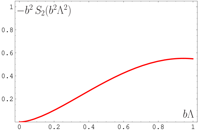
Fig. 1: Exponent of the first non-constant power correction to the Drell-Yan cross-section as a function of the impact parameter $b$.

4. Conclusions
We have focused on two specific cases – the pion form factor at leading power in $Q^{2}$ and the Drell-Yan process – which expose all the salient features of the proposed analytization methodology. On account of analytization of hadronic functions as a whole, the dispersive conjugate of the running coupling is defined unambiguously. Moreover, and even more important, one can calculate not only the power of power corrections to hadronic processes, but also their concomitant coefficients because this approach does not contain an IR renormalon ambiguity from the outset. In this way, we were able to compute explicitly the first power correction in $\frac{Q^{2}}{\Lambda^{2}}$ to the pion form factor, as well as a Sudakov-type factor to the Drell-Yan cross-section which contains the leading power correction in $b^{2}\Lambda^{2}$. Further applications and phenomenological implications of our approach will be pursued in forthcoming publications.

- (1) N. G. Stefanis, Eur. Phys. J.direct C 7 (1999) 1 [hep-ph/9911375].
- (2) D. V. Shirkov, hep-ph/0012283.
- (3) D. V. Shirkov and I. L. Solovtsov, Theor. Math. Phys. 120 (1999) 1210 [Teor. Mat. Fiz. 120 (1999) 482] [hep-ph/9909305].
- (4) G. P. Korchemsky and G. Sterman, Nucl. Phys. B 437 (1995) 415 [hep-ph/9411211].
- (5) R. Akhoury, A. Sinkovics, and M. G. Sotiropoulos, Phys. Rev. D 58 (1998) 013011 [hep-ph/9709497].
- (6) A. V. Efremov and A. V. Radyushkin, Phys. Lett. 94B (1980) 245.
- (7) G. P. Lepage and S. J. Brodsky, Phys. Rev. D 22 (1980) 2157.
- (8) D. Müller, Phys. Rev. D 49 (1994) 2525; Phys. Rev. D 51 (1995) 3855 [hep-ph/9411338].
- (9) S. Agaev, hep-ph/9611215.
- (10) S. Agaev, Mod. Phys. Lett. A 13 (1998) 2637 [hep-ph/9805278]; Eur. Phys. J. C 1 (1998) 321 [hep-ph/9611283].
- (11) D. V. Shirkov, Teor. Mat. Fiz. 119 (1999) 55 [Theor. Math. Phys. 119 (1999) 438] [hep-th/9810246]; hep-ph/0009106.
- (12) B. V. Geshkenbein and B. L. Ioffe, JETP Lett. 70 (1999) 161 [hep-ph/9906406].
- (13) A. P. Bakulev, A. V. Radyushkin, and N. G. Stefanis, Phys. Rev. D 62 (2000) 113001 [hep-ph/005085].
- (14) A. V. Radyushkin, JINR preprint E2-82-159, JINR Rapid Communications 4[78]-96, 9 (1982) [hep-ph/9907228].
- (15) N. V. Krasnikov and A. A. Pivovarov, Phys. Lett. 116B (1982) 168.
- (16) A. A. Pivovarov, Nuovo Cim. 105 A (1992) 813.
- (17) D. V. Shirkov and I. L. Solovtsov, JINR Rapid Commun. 2[76] (1996) 5 [hep-ph/9604363]; Phys. Rev. Lett. 79 (1997) 1209 [hep-ph9704333]; Phys. Lett. B 442 (1998) 344 [hep-ph/9711251]; D. V. Shirkov, Nucl. Phys. Proc. Suppl. 64 (1998) 106 [hep-ph/9708480].
- (18) A. I. Karanikas, W. Schroers, and N. G. Stefanis, in preparation.
- (19) J. Qiu and G. Sterman, Nucl. Phys. B 353 (1991) 105; ibid. B 353 (1991) 137.
- (20) H. Contopanagos and G. Sterman, Nucl. Phys. B 400 (1993) 211; ibid. B 419 (1994) 77 [hep-ph/9310313].
- (21) R. Akhoury and V. I. Zakharov, Phys. Lett. B 357 (1995) 646 [hep-ph/9504248]; Phys. Rev. Lett. 76 (1996) 2238 [hep-ph/9512433].
- (22) M. Beneke and V. M. Braun, Nucl. Phys. B 454 (1995) 253 [hep-ph/9506452].
- (23) G. P. Korchemsky and G. Marchesini, Phys. Lett. B 313 (1993) 433.
- (24) G. Sterman, Nucl. Phys. B 281 (1987) 310.
- (25) G. Curci and M. Greco, Phys. Lett. 92B (1980) 175.
- (26) J. Kodaira and L. Trentadue, Phys. Lett. 112B (1982) 66.
- (27) N. G. Stefanis, W. Schroers, and H.-Ch. Kim, Eur. Phys. J. C 18 (2000) 137 [hep-ph/0005218]; Phys. Lett. B 449 (1999) 299 [hep-ph/9807298].
- (28) I. S. Gradshteyn and I. M. Ryzhik, Table of Integrals, Series and Products (Academic Press, San Diego, 1980).
- (29) N. G. Stefanis, Mod. Phys. Lett. A 10 (1995) 1419.
- (30) J. C. Collins and D. E. Soper, Nucl. Phys. B 193 (1981) 381; Nucl. Phys. B 197, (1982) 446.