MSU-HEP-07101 CERN-TH/2000-360

Uncertainties of predictions from parton
distribution functions II: the Hessian method

J. Pumplin, D. Stump, R. Brock, D. Casey, J. Huston,
J. Kalk, H.L. Lai,^a W.K. Tung^b

Department of Physics and Astronomy

Michigan State University

East Lansing, MI 48824

^a Ming-Hsin Institute of Technology

Hsin-Chu, Taiwan

^b Theory Division, CERN

Geneva, Switzerland

We develop a general method to quantify the uncertainties of parton distribution functions and their physical predictions, with emphasis on incorporating all relevant experimental constraints. The method uses the Hessian formalism to study an effective chi-squared function that quantifies the fit between theory and experiment. Key ingredients are a recently developed iterative procedure to calculate the Hessian matrix in the difficult global analysis environment, and the use of parameters defined as components along appropriately normalized eigenvectors. The result is a set of $2d$ Eigenvector Basis parton distributions (where $d\!\approx\!16$ is the number of parton parameters) from which the uncertainty on any physical quantity due to the uncertainty in parton distributions can be calculated. We illustrate the method by applying it to calculate uncertainties of gluon and quark distribution functions, $W$ boson rapidity distributions, and the correlation between $W$ and $Z$ production cross sections.

1 Introduction

The partonic structure of hadrons plays a fundamental role in elementary particle physics. Interpreting experimental data according to the Standard Model (SM), precision measurement of SM parameters, and searches for signals of physics beyond the SM, all rely on the parton picture of hadronic beam particles that follows from the factorization theorem of Quantum Chromodynamics (QCD). The parton distribution functions (PDFs) are nonperturbative—and hence at present uncalculable—functions of momentum fraction $x$ at a low momentum transfer scale $Q_{0}$. They are determined phenomenologically by a global analysis of experimental data from a wide range of hard-scattering processes, using perturbative QCD to calculate the hard scattering and to determine the dependence of the PDFs on $Q$ by the renormalization-group based evolution equations.

Considerable progress has been made in several parallel efforts to improve our knowledge of the PDFs [1, 2, 3], but many problems remain open. In the conventional approach, specific PDF sets are constructed to represent the “best estimate” under various input assumptions, including selective variations of some of the parameters [4, 5, 6]. From these results, however, it is impossible to reliably assess the uncertainties of the PDFs or, more importantly, of the physics predictions based on them. The need to quantify the uncertainties for precision SM studies and New Physics searches in the next generation of collider experiments has stimulated much interest in developing new approaches to this problem [7, 8]. Several attempts to quantify the uncertainties of PDFs in a systematic manner have been made recently [9, 10, 11, 12, 13].

The task is difficult because of the diverse sources of experimental and theoretical uncertainty in the global QCD analysis. In principle, the natural framework for studying uncertainties is that of the likelihood function [12, 14, 15]. If all experimental measurements were available in the form of mutually compatible probability functions for candidate theory models, then the combined likelihood function would provide the probability distribution for the possible PDFs that enter the theory. From this, all physical predictions and their uncertainties would follow. Unfortunately, such ideal likelihood functions are rarely available from real experiments. To begin with, most published data sets used in global analysis provide only effective errors in uncorrelated form, along with a single overall normalization uncertainty. Secondly, published errors for some well-established experiments appear to fail standard statistical tests, e.g., the $\chi^{2}$ per degree of freedom may deviate significantly from $1.0$, making the data set quite “improbable”. In addition, when the few experiments that are individually amenable to likelihood analysis are examined together, they appear to demand mutually incompatible PDF parameters. A related problem is that the theoretical errors are surely highly correlated and by definition poorly known. All these facts of life make the idealistic approach impractical for a real-world global QCD analysis.

The problems that arise in combining a large number of diverse experimental and theoretical inputs with uncertain or inconsistent errors are similar to the problems routinely faced in analyzing systematic errors within experiments, and in averaging data from measurements that are marginally compatible [16]. Imperfections of data sets in the form of unknown systematic errors or unusual fluctuations—or both—are a common occurrence. They need not necessarily destroy the value of those data sets in a global analysis; but we must adapt and expand the statistical tools we use to analyze the data, guided by reasonable physics judgement.

In this paper we develop a systematic procedure to study the uncertainties of PDFs and their physics predictions, while incorporating all the experimental constraints used in the previous CTEQ analysis [1]. An effective $\chi^{2}$ function, called $\chi_{\mathrm{global}}^{2}$, is used not only to extract the “best fit”, but also to explore the neighborhood of the global minimum in order to quantify the uncertainties, as is done in the classic Error Matrix approach. Two key ingredients make this possible: (i) a recently established iterative procedure [17] that yields a reliable calculation of the Hessian matrix in the complex global analysis environment; and (ii) the use of appropriately normalized eigenvectors to greatly improve the accuracy and utility of the analysis.

The Hessian approach is based on a quadratic approximation to $\chi_{\mathrm{global}}^{2}$ in the neighborhood of the minimum that defines the best fit. It yields a set of PDFs associated with the eigenvectors of the Hessian, which characterize the PDF parameter space in the neighborhood of the global minimum in a process-independent way. In a companion paper, referred to here as LMM [18], we present a complementary process-dependent method that studies $\chi_{\mathrm{global}}^{2}$ as a function of whatever specific physical variable is of interest. That approach is based on the Lagrange Multiplier method [17], which does not require a quadratic approximation to $\chi_{\mathrm{global}}^{2}$, and hence is more robust; but, being focused on a single variable (or a few variables in a generalized formulation), it does not provide complete information about the neighborhood of the minimum. We use the LM method to verify the reliability of the Hessian calculations, as discussed in Sec. 5. Further tests of the quadratic approximation are described in Appendix B.

The outline of the paper is as follows. In Sec. 2 we summarize the global analysis that underlies the study, and define the function $\chi_{\mathrm{global}}^{2}$ that plays the leading role. In Sec. 3 we in explore the quality of fit in the neighborhood of the minimum. We derive the Eigenvector Basis sets, and show how they can be used to calculate the uncertainty on any quantity that depends on the parton distributions. In Sec. 4 we apply the formalism to derive uncertainties of the PDF parameters and of the PDFs themselves. In Sec. 5 we illustrate the method further by finding the uncertainties on predictions for the rapidity distribution of $W$ production, and the correlation between $W$ and $Z$ production cross sections. We summarize our results in Sec. 6. Two appendices provide details on the estimate of overall tolerance for the effective $\chi_{\mathrm{global}}^{2}$ function, and on the validity of the quadratic approximation inherent in the Hessian method. Two further appendices supply explicit tables of the coefficients that define the best fit and the Eigenvector Basis sets. The mathematical methods used here have been described in detail in [17]. Some preliminary results have also appeared in [7, 8].

2 Global QCD Analysis and Effective Chi-squared

Global $\chi^{2}$ analysis is a practical and effective way to combine a large number of experimental constraints. In this section, we describe the main features of the global QCD analysis, and explain how we quantify its uncertainties through the behavior of $\chi_{\mathrm{global}}^{2}$.

2.1 Experimental and theoretical inputs

We use the same experimental input as the CTEQ5 analysis [1]: 15 data sets on neutral-current and charged-current deep inelastic scattering (DIS), Drell-Yan lepton pair production (DY), forward/backward lepton asymmetry from $W$ production, and high $p_{T}$ inclusive jets, as listed in Table 1 of Appendix A. The total number of data points is $1295$ after cuts, such as $Q>2\,{\rm GeV}$ and $W>4\,{\rm GeV}$ in DIS, designed to reduce the influence of power-law suppressed corrections and other sources of theoretical error. The experimental precision and the information available on systematic errors vary widely among the experiments, which presents difficulties for the effort to quantify the uncertainties of the results.

The theory input is next-to-leading-order (NLO) perturbative QCD. The theory has systematic uncertainties due to uncalculated higher-order QCD corrections, including possible resummation effects near kinematic boundaries; power-suppressed corrections; and nuclear effects in neutrino data on heavy targets. These uncertainties—even more than the experimental ones—are difficult to quantify.

The theory contains free parameters $\{a_{i}\}=\{a_{1},\ldots,a_{d}\}$ defined below that characterize the nonperturbative input to the analysis. Fitting theory to experiment determines these $\{a_{i}\}$ and thereby the PDFs. The uncertainty of the result due to experimental and theoretical errors is assessed in our analysis by an assumption on the permissible range of $\Delta\chi^{2}$ for the fit, which is discussed in Sec. 2.4.

2.2 Parametrization of PDFs

The PDFs are specified in a parametrized form at a fixed low energy scale $Q_{0}$, which we choose to be $1\,{\rm GeV}$. The PDFs at all higher $Q$ are determined from these by the NLO perturbative QCD evolution equations. The functional forms we use are

$$f(x,Q_{0})=A_{0}\,x^{A_{1}}\,(1-x)^{A_{2}}\,(1+A_{3}\,x^{A_{4}})$$ (1)

with independent parameters for parton flavor combinations $u_{v}\equiv u-\bar{u}$, $d_{v}\equiv d-\bar{d}$, $g$, and $\bar{u}+\bar{d}\,$. We assume $s=\bar{s}=0.2\,(\bar{u}+\bar{d})$ at $Q_{0}$. A somewhat different parametrization for the $\bar{d}/\bar{u}$ ratio is adopted to better fit the current data:

$$\bar{d}(x,Q_{0})/\bar{u}(x,Q_{0})=B_{0}\,x^{B_{1}}\,(1-x)^{B_{2}}\;+\;(1+B_{3}x)\,(1-x)^{B_{4}}\;.$$ (2)

The specific functional forms are not crucial, as long as the parametrization is flexible enough to include the behavior of the true—but unknown—PDFs at the level of accuracy to which they can be determined. The parametrization should also provide additional flexibility to model the degrees of freedom that remain indeterminate. On the other hand, too much flexibility in the parametrization leaves some parameters poorly determined at the minimum of $\chi^{2}$. To avoid that problem, some parameters in the present study were frozen at particular values.

The number of free parameters has increased over the years, as the accuracy and diversity of the global data set has gradually improved. A useful feature of the Hessian approach is the feedback it provides to aid in refining the parametrization, as we discuss in Sec. 4.1. The current analysis uses a total of $d\!=\!16$ independent parameters, referred to generically as $\{a_{i}\}$. Their best-fit values, together with the fixed ones, are listed in Table 3 of Appendix C. (Some of the fit parameters $a_{i}$ are defined by simple functions of their related PDF shape parameters $A_{i}$ or $B_{i}$, as indicated in the table, to keep their relevant magnitudes in a similar range, or to enforce positivity of the input PDFs, etc.) The set of fit parameters $\{a_{i}\}$ could also include parameters associated with correlated experimental errors, such as an unknown normalization error that is common to all of the data points in a particular experiment; however, such parameters were kept fixed for simplicity in this initial study. The QCD coupling was similarly fixed at $\alpha_{s}(M_{Z})=0.118\,$.

2.3 Effective chi-squared function

Our analysis is based on an effective global chi-squared function that measures the quality of the fit between theory and experiment:

$$\chi_{\mathrm{global}}^{2}=\sum_{n}\,w_{n}\,\chi_{n}^{2}$$ (3)

where $n$ labels the $15$ different data sets.

The weight factors $w_{n}$ in (3), with default value $1$, are a generalization of the selection process that must begin any global analysis, where one decides which data sets to include ($w\!=\!1$) or exclude ($w\!=\!0$). For instance, we include neutrino DIS data (because it contains crucial constraints on the PDFs, although it requires model-dependent nuclear target corrections); but we exclude direct photon data (which would help to constrain the gluon distribution, but suffers from delicate sensitivity to $k_{\perp}$ effects from multiple soft gluon emission). The $w_{n}$ can be used to emphasize particular experiments that provide unique physical information, or to de-emphasize experiments when there are reasons to suspect unquantified theoretical or experimental systematic errors (e.g. in comparison to similar experiments). Subjectivity such as this choice of weights is not covered by Gaussian statistics, but is a part of the more general Bayesian approach; and is in spirit a familiar aspect of estimating systematic errors within an experiment, or in averaging experimental results that are marginally consistent.

The generic form for the individual contributions in Eq. (3) is

$$\chi_{n}^{2}=\sum_{I}\left(\frac{D_{nI}-T_{nI}}{\sigma_{nI}}\right)^{2}$$ (4)

where $T_{nI}$, $D_{nI}$, and $\sigma_{nI}$ are the theory value, data value, and uncertainty for data point $I$ of data set (or “experiment”) $n$. In practice, Eq. (4) is generalized to include correlated errors such as overall normalization factors; or even the full experimental error correlation matrix if it is available [18].

The value of $\chi_{\mathrm{global}}^{2}$ depends on the PDF set, which we denote by $S$. We stress that $\chi_{\mathrm{global}}^{2}(S)$ is an “effective $\chi^{2}\,$”, whose purpose is to measure how well the data are fit by the theory when the PDFs are defined by the parameter set $\{a_{i}(S)\}$. We use $\chi_{\mathrm{global}}^{2}(S)$ to study how the quality of fit varies with the PDF parameters; but we do not assign a priori statistical significance to specific values of it—e.g., in the manner that would be appropriate to an ideal chi-squared distribution—since the experimental and theoretical inputs are often far from being ideal, as discussed earlier.

2.4 Global minimum and its neighborhood

Having specified the effective $\chi^{2}$ function, we find the parameter set that minimizes it to obtain a “best estimate” of the true PDFs. This PDF set is denoted by $S_{0}$. The parameter values that characterize $S_{0}$ are listed in Table 3 of Appendix C.

To study the uncertainties, we must explore the variation of $\chi_{\mathrm{global}}^{2}$ in the neighborhood of its minimum, rather than focusing only on $S_{0}$ as has been done in the past. Moving the parameters away from the minimum increases $\chi_{\mathrm{global}}^{2}$ by an amount $\Delta\chi^{2}_{\mathrm{global}}$. It is natural to define the relevant neighborhood of the global minimum as

$$\Delta\chi_{\mathrm{global}}^{2}\,\leq\,T^{2}$$ (5)

where $T$ is a tolerance parameter. The Hessian formalism developed in the next section (Sec. 3) provides a reliable and efficient method of calculating the variation of all predictions of PDFs in this neighborhood, as long as $T$ is within the range where a quadratic expansion of $\chi_{\mathrm{global}}^{2}$ in terms of the PDF parameters is adequate.

In order to quantify the uncertainties of physical predictions that depend on PDFs, one must choose the tolerance parameter $T$ to correspond to the region of “acceptable fits”. Broadly speaking, the order of magnitude of $T$ for our choice of $\chi_{\mathrm{global}}^{2}$ is already suggested by self-consistency considerations: Our fundamental assumption—that the 15 data sets used in the global analysis are individually acceptable and mutually compatible, in spite of departures from ideal statistical expectations exhibited by some of the individual data sets, as well as signs of incompatibility between some of them if the errors are interpreted according to strict statistical rules [12]—must, in this effective $\chi^{2}$ approach, imply a value of $T$ substantially larger than that of ideal expectations. More quantitatively, estimates of $T$ have been carried out in the companion paper LMM [18], based on the comparison of $\Delta\chi_{\mathrm{global}}^{2}$ with detailed studies of experimental constraints on specific physical quantities. The estimates of $T$ will be discussed more extensively in Sec. 5, where applications are presented, and in Appendix A. For the development of the formalism in the next section, it suffices to know that (i) the order of magnitude of these estimates is

$$T\approx 10\;{\rm to}\;15\;;$$ (6)

and (ii) the master formulas given in Sec. 3.4 show that all uncertainties are proportional to $T$, so that results derived for a particular value of $T$ can easily be scaled to other estimates of $T$ if desired.

3 The Hessian formalism

The most efficient approach to studying uncertainties in a global analysis of data is through a quadratic expansion of the $\chi^{2}$ function about its global minimum. This is the well known Error Matrix or Hessian method. Although the method is standard, its application to PDF analysis has, so far, been hindered by technical problems created by the complexity of the theoretical and experimental inputs. Those technical problems have recently been overcome [17].

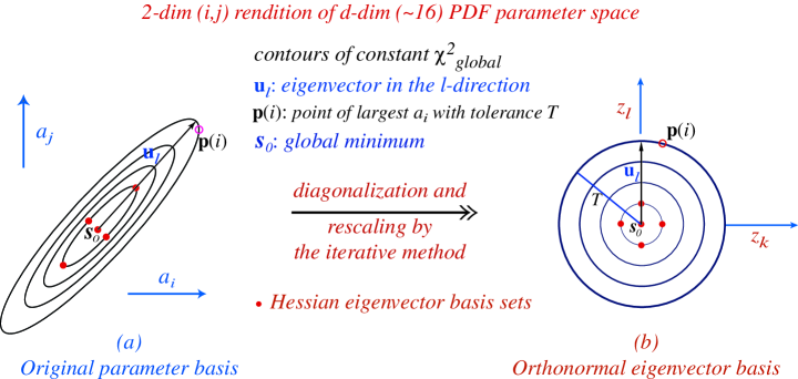
Figure 1: Illustration of the basic ideas of our implementation of the Hessian method. An iterative procedure [17] diagonalizes the Hessian matrix and rescales the eigenvectors to adapt the step sizes to their natural scale. The solid points represent the resulting eigenvector basis PDFs described in Sec. 3.3. Point $\mathbf{p(i)}$ is explained in Sec. 4.1.

The Hessian matrix is the matrix of second derivatives of $\chi^{2}$ at the minimum. In our implementation, the eigenvectors of the Hessian matrix play a central role. They are used both for accurate evaluation of the Hessian itself, via the iterative method of [17], and to produce an Eigenvector Basis set of PDFs from which uncertainties of all physical observables can be calculated. These basis PDFs provide an optimized representation of the parameter space in the neighborhood of the minimum $\chi^{2}$.

The general idea of our approach is illustrated conceptually in Fig. 1. Every PDF set $S$ corresponds to a point in the $d$-dimensional PDF parameter space. It can be specified by the original parton shape parameters $\{a_{i}(S)\}$ defined in Sec. 2.2, as illustrated in Fig. 1(a); or by the Eigenvector Basis coordinates $\{z_{k}(S)\}$, which specify the components of $S$ along the Eigenvector Basis PDFs that will be introduced in Sec. 3.3, as illustrated in Fig. 1(b). The solid points in both (a) and (b) represent the basis PDF sets.

3.1 Quadratic approximation and the Hessian matrix

The standard error matrix approach begins with a Taylor series expansion of $\chi_{\mathrm{global}}^{2}(S)$ around its minimum $S_{0}$, keeping only the leading terms. This produces a quadratic form in the displacements from the minimum:

$$\Delta\chi^{2}\,=\,\chi^{2}-\chi_{0}^{\,2}\,=\,\sum_{i=1}^{d}\sum_{j=1}^{d}\,H_{ij}\,(a_{i}-a^{0}_{i})\,(a_{j}-a^{0}_{j})$$ (7)

where $\chi_{0}^{\,2}=\chi^{2}(S_{0})$ is the value at the minimum, $\{a_{j}^{0}\}=\{a_{j}(S_{0})\}$ is its location, and $\{a_{j}\}=\{a_{j}(S)\}$. We have dropped the subscript “global” on $\chi^{2}$ for simplicity. We also suppress the PDF argument $(S)$ in $\chi^{2}$ and $\{a_{i}\}$ here and elsewhere for brevity.

The Hessian matrix $H_{ij}$ has a complete set of orthonormal eigenvectors $v_{ik}$ defined by

$$\sum_{j=1}^{d}\,H_{ij}\,v_{jk} = \epsilon_{k}\,v_{ik}$$ (8)

$$\sum_{i=1}^{d}\,v_{i\ell}\,v_{ik} = \delta_{\ell k}\;,$$ (9)

where $\{\epsilon_{k}\}$ are the eigenvalues and $\delta_{\ell k}$ is the unit matrix. Displacements from the minimum are conveniently expressed in terms of the eigenvectors by

$$a_{i}-a^{0}_{i}=\sum_{k=1}^{d}\,v_{ik}\,s_{k}\,z_{k}\;,$$ (10)

where scale factors $s_{k}$ are introduced to normalize the new parameters $z_{k}$ such that

$$\Delta\chi^{2}\,=\,\sum_{k=1}^{d}\,z_{k}^{\,2}\;.$$ (11)

With this normalization, the relevant neighborhood (5) of the global minimum corresponds to the interior of a hypersphere of radius $T$:

$$\sum_{k=1}^{d}\,z_{k}^{\,2}\,\leq\,T^{2}\;.$$ (12)

In the ideal quadratic approximation, the scale factors $s_{k}$ would be equal to $\sqrt{1/\epsilon_{k}}\,$. However, if $\chi^{2}$ is not perfectly quadratic, then $s_{k}$ differs somewhat from $\sqrt{1/\epsilon_{k}}\,$, as explained in Appendix B.

The transformation (10) is illustrated conceptually in Fig. 1, where $\{k,\ell\}$ label two of the eigenvector directions. One of the eigenvectors $\mathbf{v}_{\ell}$ is shown both in the original parameter basis and in the normalized eigenvector basis.

3.2 Eigenvalues of the Hessian matrix

The square of the distance in parameter space from the minimum of $\chi^{2}$ is

$$\sum_{i=1}^{d}\,(a_{i}-a_{i}^{0})^{2}\,=\,\sum_{k=1}^{d}\,(s_{k}\,z_{k})^{2}$$ (13)

by (9)–(10). Because $s_{k}\approx\sqrt{1/\epsilon_{k}}$, an eigenvector with large eigenvalue $\epsilon_{k}$ therefore corresponds to a “steep direction” in $\{a_{i}\}$ space, i.e., a direction in which $\chi^{2}$ rises rapidly, making the parameters tightly constrained by the data. The opposite is an eigenvector with small $\epsilon_{k}$, which corresponds to a “shallow direction”, for which the criterion $\Delta\chi^{2}\leq T^{2}$ permits considerable motion—as is the case for $\mathbf{v}_{\ell}$ illustrated in Fig. 1.

The distribution of eigenvalues, ordered from largest to smallest, is shown in Fig. 2. Interestingly, the distribution is approximately linear in $\,\log\epsilon\,$. The eigenvalues span an enormous range, which is understandable because the large global data set includes powerful constraints—particularly on combinations of parameters that control the quark distributions at moderate $x$—leading to steep directions; while free parameters have purposely been added to (1)–(2) to the point where some of them are at the edge of being unconstrained by the data, leading to shallow directions.

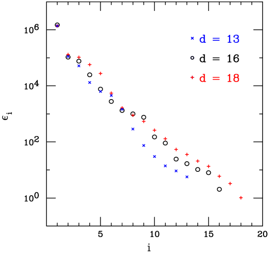
Figure 2: Distribution of eigenvalues of the Hessian matrix for fits using $d=13$, $16$ (standard), and $18$ free PDF parameters.

Fig. 2 also shows how the range of eigenvalues expands or contracts if the number of adjustable parameters is changed: the 16-parameter fit is the standard one used in most of this paper; the 18-parameter fit is defined by allowing $A_{1}^{u_{v}}\neq A_{1}^{d_{v}}$ and $A_{3}^{g}\neq 0$ with $A_{4}^{g}=6$; the 13-parameter fit is defined by $A_{4}^{u_{v}}=A_{4}^{d_{v}}=1$ and $A_{3}^{\bar{d}+\bar{u}}=0$. The range spanned by the eigenvalues increases with the dimension $d$ of the parameter space (roughly as $\,\log(\epsilon_{1}/\epsilon_{d})\propto d^{0.4}\,$).

The large ($10^{6}\!:\!1$) range spanned by the eigenvalues makes the smaller eigenvalues and their eigenvectors very sensitive to fine details of the Hessian matrix, making it difficult to compute $H_{ij}$ with sufficient accuracy. This technical problem hindered the use of Hessian or Error Matrix methods in global QCD analysis in the past. The problem has been tamed by an iterative method introduced in [17], which computes the eigenvalues and eigenvectors by successive approximations that converge even in the presence of numerical noise and non-quadratic contributions to $\chi^{2}\,$.

The Hessian method relies on the quadratic approximation (7) to the effective $\chi^{2}$ function. We have extensively tested this approximation in the neighborhood of interest by comparing it with the exact $\chi^{2}_{\mathrm{global}}$. The results are satisfactory, as shown in Appendix B, which also explains how the approximation is improved by adjusting the scale factors $s_{k}$ for the shallow directions.

3.3 PDF Eigenvector Basis sets $S_{\ell}^{\pm}$

The $k^{\rm th}$ eigenvector of the Hessian matrix has component $v_{ik}$ along the $i^{\rm th}$ direction in the original parameter space, according to (8). Thus $v_{ik}$ is the orthogonal matrix that transforms between the original parameter basis and the eigenvector basis. For our application, it is more convenient to work with coordinates $\{z_{k}\}$ that are normalized by the scale factors $\{s_{k}\}$ of (10), rather than the “raw” coordinates of the eigenvector basis. Thus we use the matrix

$$M_{ik}\equiv v_{ik}\,s_{k}$$ (14)

rather than $v_{ik}$ itself. $M_{ik}$ defines the transformation between the two descriptions that are depicted conceptually in Fig. 1:

$$a_{i}-a^{0}_{i}=\sum_{k=1}^{d}\,M_{ik}\,z_{k}\;.$$ (15)

It contains information about the physics in the global fit, together with information related to the choice of parametrization, and is a good object to study for insight into how the parametrization might be improved, as we discuss in Sec. 4.1.

The eigenvectors provide an optimized orthonormal basis in the PDF parameter space, which leads to a simple parametrization of the parton distributions in the neighborhood of the global minimum $S_{0}$. In the remainder of this section, we show how to construct these Eigenvector Basis PDFs $\{S_{\ell}^{\pm},\ell=1,\ldots,d\}\,$; and in the following subsection, we show how they can be used to calculate the uncertainty of any desired variable $X(S)$.

The Eigenvector Basis sets $S_{\ell}^{\pm}$ are defined by displacements of a standard magnitude $t$ “up” or “down” along each of the $d$ eigenvector directions. Their coordinates in the $z$-basis are thus

$$z_{k}(S_{\ell}^{\pm})=\pm\,t\,\delta_{k\ell}\;.$$ (16)

More explicitly, $S_{1}^{+}$ is defined by $\left(z_{1},\dots,z_{d}\right)=\left(t,0,\dots,0\right)$, etc. We make displacements in both directions along each eigenvector to improve accuracy; which direction is called “up” is totally arbitrary. As a practical matter, we choose $t\!=\!5$ for the displacement distance. This choice improves the accuracy of the quadratic approximation by working with displacements that have about the same size as those needed in applications.

The $\{a_{i}\}$ parameters that specify the Eigenvector Basis sets $S_{\ell}^{\pm}$ are given by

$$a_{i}(S_{\ell}^{\pm})\,-\,a_{i}^{0}\,=\,\pm\,t\,M_{i\ell}$$ (17)

by (15)–(16). Hence

$$a_{i}(S_{\ell}^{+})-a_{i}(S_{\ell}^{-})\,=\,2\,t\,M_{i\ell}\;.$$ (18)

Interpreted as a difference equation, this shows directly that the element $M_{i\ell}$ of the transformation matrix is equal to the gradient of parameter $a_{i}$ along the direction of $z_{\ell}$.

Basis PDF sets along two of the eigenvector directions are illustrated conceptually in Fig. 1 (a) and (b) as solid points displaced from the global minimum set $S_{0}$. The coefficients that specify all of the sets $S_{\ell}^{\pm}$ are listed in Table 4 of Appendix D.

3.4 Master equations for calculating uncertainties using the Eigenvector Basis sets $\{S_{\ell}^{\pm}\}$

Let $X(S)$ be any variable that depends on the PDFs. It can be a physical quantity such as the $W$ production cross section; or a particular PDF such as the gluon distribution at specific $x$ and $Q$ values; or even one of the PDF parameters $a_{i}$. All of these cases will be discussed as examples in Sections 4 and 5.

The best-fit estimate for $X$ is $X^{0}\!=\!X(S_{0})$. To find the uncertainty, it is only necessary to evaluate $X$ for each of the $2d$ sets $\{S_{\ell}^{\pm}\}$. The gradient of $X$ in the $z$-representation can then be calculated, using a linear approximation that is essential to the Hessian method, by

$$\frac{\partial X}{\partial z_{k}}\,=\,\frac{X(S_{k}^{+})-X(S_{k}^{-})}{2\,t}$$ (19)

where $t$ is the scale used to define $\{S_{\ell}^{\pm}\}$ in (16). It is useful to define

$$D_{k}(X) = X(S_{k}^{+})-X(S_{k}^{-})$$ (20)

$$D(X) = \left(\,\sum_{k=1}^{d}\,[D_{k}(X)]^{2}\right)^{\!1/2}$$ (21)

$$\widehat{D}_{k}(X) = D_{k}(X)/D(X)\;,$$ (22)

so that $D_{k}(X)$ is a vector in the gradient direction and $\widehat{D}_{k}(X)$ is the unit vector in that direction.

The gradient direction is the direction in which $X$ varies most rapidly, so the largest variations in $X$ permitted by (12) are obtained by displacement from the global minimum $S_{0}$ in the gradient direction by a distance $\pm T$. Hence

$$\Delta X\,=\,\sum_{k=1}^{d}\,(T\,\widehat{D}_{k})\frac{\partial X}{\partial z_{k}}\;.$$ (23)

From this, using (19)–(22), we obtain the master equation for calculating uncertainties,

$$\framebox{\mbox{\mbox{$\displaystyle\;\Delta X\,=\,\frac{T}{2t}\,D(X)\;$}}}\;.$$ (24)

This equation is applied to obtain numerical results in Sections 4 and 5.

For applications, it is often important also to construct the PDF sets $S_{X}^{+}$ and $S_{X}^{-}$ that achieve the extreme values $X=X^{0}\pm\Delta X$. Their $z$-coordinates are

$$z_{k}(S_{X}^{\pm})\,=\,\pm\,T\,\widehat{D}_{k}(X)\;,$$ (25)

which follows from the derivation of (24). Their physical parameters $\{a_{i}\}$ then follow from Eqs.(15) and (18):

$$\framebox{\mbox{\mbox{$\displaystyle\;a_{i}(S_{X}^{\pm})-a_{i}^{0}\,=\,{\frac{\pm T}{2t}}\,\sum_{k=1}^{d}\,\widehat{D}_{k}(X)\,[a_{i}(S_{k}^{+})-a_{i}(S_{k}^{-})]\;$}}}\;.$$ (26)

In practice, we calculate the parameters for $S_{X}^{+}$ and $S_{X}^{-}$ by applying (26) directly to the parton shape parameters $\,\ln A_{0}^{u_{v}}$, $A_{1}^{u_{v}}$,…listed in Table 4, except that the normalization factors $A_{0}^{u_{v}}$, $A_{0}^{d_{v}}$, and $A_{0}^{g}$ are computed from the momentum sum rule and quark number sum rules

$$\sum_{i}\int_{0}^{1}\!x\,f_{i}(x)\,dx\,=\,1$$ (27)

$$\int_{0}^{1}\!u_{v}(x)\,dx\,=\,2\;,\qquad\int_{0}^{1}\!d_{v}(x)\,dx\,=\,1$$ (28)

to ensure that those sum rules are satisfied exactly.

4 Uncertainties of Parton Distributions

4.1 Uncertainties of the PDF parameters $\{a_{i}\}$

As a useful as well as illustrative application of the general formalism, let us find the uncertainties on the physical PDF parameters $a_{i}$. We only need to follow the steps of Sec. 3.4. Letting $X=a_{i}$ for a particular $i$, Eqs. (20) and (18) give

$$D_{k}(a_{i})=\,a_{i}(S_{k}^{+})-a_{i}(S_{k}^{-})=2t\,M_{ik}\;.$$ (29)

The uncertainty on $a_{i}$ in the global analysis follows from the master equation (24):

$$\Delta a_{i}\,=\,T\left(\sum_{k}M_{ik}^{\,2}\right)^{\,1/2}\;.$$ (30)

The parameter sets $\{a_{j}(a_{i}^{+})\}$ and $\{a_{j}(a_{i}^{-})\}$ that produce the extreme values of $a_{i}$ can be found using (26). In the conceptual Fig. 1, the parton distribution set with the largest value of $a_{i}$ for $\Delta\chi_{\mathrm{global}}^{2}=T^{2}$ is depicted as point $\mathbf{p(i)}$.

The uncertainties $\{\Delta a_{i}\}$ of the standard parameter set, calculated from (30) with $T=5$ are listed along with the central values $\{a_{i}^{0}\}$ in Table 3. To test the quadratic approximation, asymmetric errors are also listed. These are defined by displacements in the gradient direction (29) that are adjusted to make $\Delta\chi^{2}$ exactly equal to $T^{2}=25$. They agree quite well with the errors calculated using (30), which shows that the quadratic approximation is adequate for our purposes.

Table 3 also lists the components of the displacement vectors $z_{k}(a_{i}^{+})$ of (25), which have been renormalized to $\sum z_{k}^{\,2}=1$. These reveal which features of the PDFs are governed most strongly by specific eigenvector directions. The table is divided into sections according to the various flavor combinations that are parametrized. One can see for example that the flattest direction $z_{16}$ is strongly related to the gluon parameters $A_{1}^{g}$ and $A_{2}^{g}$, confirming that the gluon distribution at $Q_{0}=1\,\mathrm{GeV}$ is a highly uncertain aspect of the PDFs. The second-flattest direction $z_{15}$ relates mainly to the $\bar{d}/\bar{u}$ ratio, as seen by the large components along $z_{15}$ for $B_{0}^{\bar{d}/\bar{u}}$ and $B_{1}^{\bar{d}/\bar{u}}$. Meanwhile, the steepest direction $z_{1}$ mainly influences the valence quark distribution, via $A_{1}^{u_{v}}$.

All of the parametrized aspects of the PDFs at $Q_{0}$, namely $u_{v}$, $d_{v}$, $g$, $\bar{d}+\bar{u}$, and $\bar{d}/\bar{u}$ receive substantial contributions from the four flattest directions $13$–$16$, which shows that the current global data set could not support the extraction of much finer detail in the PDFs. This can be confirmed by noting that the error ranges of the individual parameters $a_{i}$ are not small.

4.2 Uncertainties of the PDFs

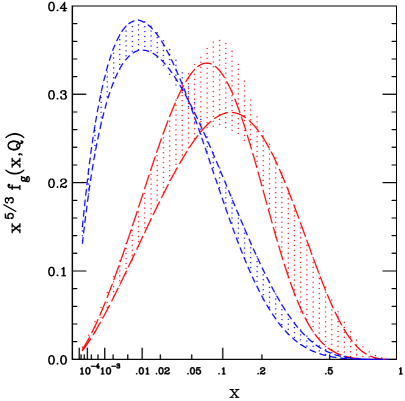
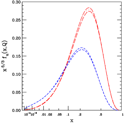
Figure 3: Two extreme gluon distributions (left) and $u$-quark distributions (right) for $Q\!=\!2\,{\rm GeV}$ (long dash) and $Q\!=\!100\,{\rm GeV}$ (short dash) with $T\!=\!10$. Each curve is calculated to give the minimum or maximum value for some particular $x$. The entire allowed region, which is the envelope of all such curves, is shaded.

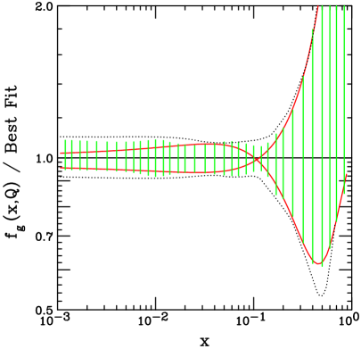
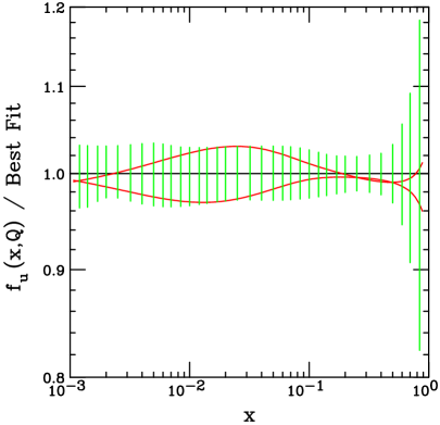
Figure 4: Ratio of gluon (left) and $u$-quark (right) distributions to Best Fit $S_{0}$ at $Q=10\,{\rm GeV}$.

The uncertainty range of the PDFs themselves can also be explored using the eigenvector method. For example, letting the gluon distribution $g(x,Q)$ at some specific values of $x$ and $Q$ be the variable $X$ that is extremized by the method of Sec. 3.4 leads to the extreme gluon distributions shown in the left-hand side of Fig. 3. The envelope of such curves, obtained by extremizing at a variety of $x$ values at fixed $Q$, is shown by the shaded region, which is defined by $T\!=\!10$, i.e., by allowing $\chi_{\rm{global}}^{2}$ up to $100$ above its minimum value.

The right-hand side of Fig. 3 similarly shows the allowed region and two specific cases for the $u$-quark distribution. The uncertainty is much smaller than for the gluon, reflecting the large amount of experimental data included in the global analysis that is sensitive to the $u$ quark through the square of its electric charge.

The dependence on $x$ in these figures is plotted as a function of $x^{1/3}$ to better display the region of current experimental interest. The values are weighted by a factor $x^{5/3}$, which makes the area under each curve proportional to its contribution to the momentum sum rule. Note that the uncertainty decreases markedly with increasing $Q$ as a result of evolution. Also note that the gluon distribution is large and fairly well determined at smaller $x$ values and large $Q$—the region that will be vital for physics at the LHC.

Figure 4 displays similar information for $Q=10\,{\rm GeV}$, expressed as the fractional uncertainty as a function of $\,\log x$. It shows that the gluon distribution becomes very uncertain at large $x$, e.g., $x\!>\!0.25\,$. (At $x\!>\!0.6$, where the distribution is extremely small, the lower envelope of fractional uncertainty begins to rise. This is an artifact of the parametrization with $A_{3}^{g}=0$; e.g., making the parametrization more flexible by freeing $A_{3}^{g}$ with $A_{4}^{g}=6$ leads to a broader allowed range indicated by the dotted curves.)

The boundaries of the allowed regions for the PDFs are not themselves possible shapes for the PDFs, since if a particular distribution is extremely high at one value of $x$, it will be low at other values. This can be seen most clearly in the gluon distributions of Figs. 3 and 4, where the extreme PDFs shown push the envelope on the high side in one region of $x$, and on the low side in another.

5 Uncertainties of Physical Predictions

In applying the Hessian method to study the uncertainties of physical observables due to PDFs, it is important to understand how the predictions depend on the tolerance parameter $T$, and how well $T$ can be determined. We discuss these issues first, and then proceed to illustrate the utility of this method by examining the predictions for the rapidity distribution of $W$ and $Z$ boson production as well as the correlation of $W$ and $Z$ cross-sections in $p\bar{p}$ collisions.

First, note that the uncertainties of all predictions are linearly dependent on the tolerance parameter $T$ in the Hessian approach, by the master formula (24); hence they are easily scalable. The appropriate value of $T$ is determined, in principle, by the region of “acceptable fits” or “reasonable agreement with the global data sets” in the PDF parameter space. Physical quantities calculated from PDF sets within this region will range over the values that can be considered “likely” predictions. The language used here is intentionally imprecise, because as discussed in the introductory sections, the experimental and theoretical input to the function $\chi_{\mathrm{global}}^{2}$ in the global analysis—in particular the unknown systematic errors reflected in apparent abnormalities of some reported experimental errors as well as incompatibilities between some data sets—makes it difficult to assign an unambiguous value to $T$. However, as mentioned in Sec. 2.4, self-consistency considerations inherent in our basic assumption that the 15 data sets used in the global analysis are acceptable and compatible, in conjunction with the detailed comparison to experiment conducted in LMM [18] using the same $\chi_{\mathrm{global}}^{2}$ function, yield a best estimate of $T\approx 10\;{\rm to}\;15$ (Eq. 6). Details of these considerations are discussed in Appendix A.

Of the estimates of $T$ described there, the most quantitative one is based on the algorithm of LMM [18] to combine $90$% confidence level error bands from the 15 individual data sets for any specific physical variable such as the total production cross section of $W$ or $Z$ at the Tevatron or LHC. (Cf. Appendix A for a summary, and LMM [18] for the detailed analysis.) For the case of $\sigma_{W}^{\mathrm{TeV}}$, the uncertainty according to the specific algorithm is $\pm 4$%, corresponding to $T\sim 13$. With our working hypothesis $T\approx 10$ – $15$, the range of the uncertainty of $\sigma_{W}^{\mathrm{TeV}}$ will be $\pm 3.3\%$ to $\pm 4.9\%$.

The numerical results on applications presented in the following subsections are obtained with the same choice of $T$ as in Sec. 4, i.e. $T=10$. Bearing in mind the linear dependence of the uncertainties on $T$, one can easily scale these up by the appropriate factor if a more conservative estimate for the uncertainty of any of the physical quantities is desired. We should also note that the experimental data sets used in this analysis are continuously evolving. Some data sets (cf. Table 1 in Appendix A) will soon be updated (H1, ZEUS) or replaced (CCFR). In addition, theoretical uncertainties have yet to be systematically studied and incorporated. Therefore, the specific results presented in this paper should be considered more as a demonstration of the method rather than definitive predictions. The latter will be refined as new and better inputs become available.

5.1 Rapidity distribution for W production

Figure 5 shows the predicted rapidity distribution $d\sigma/dy$ for $W^{+}$ production in $p\bar{p}$ collisions at $\sqrt{s}=1.8\,{\rm TeV}$. The cross section is not symmetric in $y$ because of the strong contribution from the valence $u$-quark in the proton—indeed, the forward/backward asymmetry produces an observable asymmetry in the distribution of leptons from $W$ decay, which provides an important handle on flavor ratios in the current global analysis.

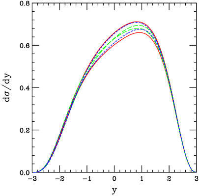
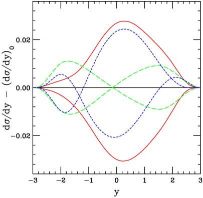
Figure 5: Left: Predicted rapidity distribution for $p\bar{p}\to W^{+}\,+\,X$ at $\sqrt{s}=1.8\,{\rm TeV}$. The curves are extreme predictions for the integrated cross section $\sigma$ (solid), or the rapidity moments $\langle y\rangle$ (long dash), or $\langle y^{2}\rangle$ (short dash). Right: same except the Best Fit prediction is subtracted to show the details better.

The left-hand side of Fig. 5 shows the six rapidity distributions that give the extremes (up or down) of the integrated cross section $\sigma=\int\frac{d\sigma}{dy}\,dy$, the first moment $\langle y\rangle$, or the second moment $\langle y^{2}\rangle$, as calculated using the Hessian formalism for $T\!=\!10$. To show the differences more clearly, the right-hand side shows the difference between each of these rapidity distributions and the Best Fit distribution.

Figure 6 shows three of the same difference curves as in Fig. 5 along with results obtained using the Lagrange Multiplier method of LMM [18]. The good agreement shows that the Hessian formalism, with its quadratic approximation (7), works well at least for this application.

Figure 7 shows the same three curves from Fig. 5, together with 6 random choices of the PDFs with $\Delta\chi_{\mathrm{global}}^{2}=100$. These random sets were obtained by choosing random directions in $\{z_{i}\}$ space and displacing the parameters from the minimum in those directions until $\chi_{\mathrm{global}}^{2}$ has increased by $100$. Note that none of this small number of random sets give good approximations to the three extreme curves. This is not really surprising, since the extrema are produced by displacements in specific (gradient) directions; and in 16-dimensional space, the component of a random unit vector along any specific direction is likely to be small. But it indicates that producing large numbers of random sets would at best be an inefficient way to unearth the extreme behaviors.

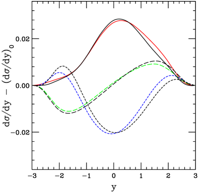
Figure 6: Comparison with Lagrange Multiplier method: Three of the six curves from Fig. 5 (corresponding to maximum $\sigma$, $\langle y\rangle$, or $\langle y^{2}\rangle$) are shown, together with the result of the exact LM method for $\Delta\chi_{\mathrm{global}}^{2}=100$.

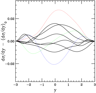
Figure 7: Comparison with random methods: Three of the six curves from Fig. 5 (corresponding to maximum $\sigma$, $\langle y\rangle$, or $\langle y^{2}\rangle$ for $\Delta\chi_{\mathrm{global}}^{2}=100$) are shown, together with results from PDF sets that are obtained by displacement in 6 random directions of $\{z_{i}\}$ space by $\Delta\chi_{\mathrm{global}}^{2}=100$.

5.2 Correlation between W and Z cross sections

One can ask what are the error limits on two quantities $X$ and $Y$ simultaneously, according to the $\Delta\chi_{\mathrm{global}}^{2}\!<T^{2}$ criterion. In the Hessian approximation, the boundary of the allowed region is an ellipse [17]. The ellipse can be expressed elegantly in a “Lissajous figure” form

$$X = X^{0}\,+\,\Delta X\,\sin(\theta+\phi)$$

$$Y = Y^{0}\,+\,\Delta Y\,\sin(\theta)\;,$$ (31)

where $0<\theta<2\pi$ traces out the boundary. The shape of the ellipse is governed by the phase angle $\phi$, which is given by the dot product between the gradient vectors for $X$ and $Y$ in $\{z_{k}\}$ space:

$$\cos\phi=\sum_{k=1}^{d}\,\widehat{D}_{k}(X)\,\widehat{D}_{k}(Y)\;,$$ (32)

where $\widehat{D}_{i}(X)$ and $\widehat{D}_{i}(Y)$ are defined by (22).

As an example of this, $T\!=\!10$ error limits for $W^{\pm}$ and $Z^{0}$ production at the Tevatron are shown in Fig. 8. The error limits on the separate predictions for these cross sections are each about $3.3\%$ for $T\!=\!10$. The predictions are strongly correlated ($\cos\phi=0.60$), in part because the same quark distributions—in different combinations—are responsible for both $W$ and $Z$ production, and in part because the uncertainties of all the quark distributions are negatively correlated with the more uncertain gluon distribution, and hence positively correlated with each other.

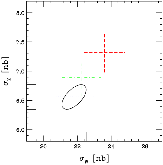
Figure 8: Error ellipse for predicted $W$ and $Z$ boson production in $p\bar{p}$ collisions at $1.8\,{\rm TeV}$. The error limit ($T\!=\!10$) of the prediction is the interior of the ellipse. Error bars show data from DØ (dotted) and CDF (dashed). The dot-dash error bars show the result of reinterpreting the CDF data by using the same assumption for luminosity as DØ [31].

The $W$ and $Z$ cross sections from CDF (dashed) and DØ (dotted) are also shown in Fig. 8 [31]. (The measured quantities $\sigma_{W}\cdot B_{W\to e\nu}$ and $\sigma_{Z}\cdot B_{Z\to e^{+}e^{-}}$ were converted to $\sigma_{W}$ and $\sigma_{Z}$ using world average values for the branching ratios [16]; the measured CDF and DØ branching ratios for $W$ agree with the world average to within about $1\%$.) The data points are shown in the form of error bars defined by combining statistical and systematic errors (including the errors in decay branching ratios) in quadrature. The errors in these measurements are also highly correlated, in part through the uncertainty in overall luminosity which both cross sections are proportional to—so the experimental points would also be better represented by ellipses. The two experiments in fact use different assumptions for the inelastic $p\bar{p}$ cross section which measures the luminosity: CDF uses its own measurement, while DØ uses the world average. The dot-dashed data point shows the result of reinterpreting the CDF point by scaling the luminosity down by a factor $1.062$ to correspond to the world average $p\bar{p}$ cross section [31].

6 Summary and Concluding Remarks

Experience over the past two decades has shown that minimizing a suitably defined $\chi_{\mathrm{global}}^{2}$ is an effective way to extract parton distribution functions consistent with experimental constraints in the PQCD framework. The goal of this paper has been to expand the analysis to make quantitative estimates of the uncertainties of PDFs and their predictions, by examining the behavior of $\chi_{\mathrm{global}}^{2}$ in the neighborhood of the minimum. The techniques developed in Ref. [17] allow us to apply the traditional error matrix approach reliably in the global analysis environment. The eigenvectors of the Hessian (inverse of the error matrix) play a crucial role, both in the adaptive procedure to accurately calculate the Hessian itself, and in the derivation of the master formula (24) for determining the uncertainties of parton distributions and their predictions.

Our principal results are: (i) the formalism developed in Sec. 3.4, leading to the master formulas; and (ii) the Best Fit parton distribution set $S_{0}$ plus the $2d$ Eigenvector Basis sets $S_{k}^{\pm}$ presented in Sec. 3.3, which are used in applications of the master formula. The uncertainties are proportional to $T$, the tolerance parameter for $\Delta\chi_{\mathrm{global}}^{2}$. We present several estimates, based on current experimental and theoretical input, that suggest $T$ is in the range $10$ – $15$. It is important to note, however, that this estimate can, and should, be refined in the near future. First, several important data sets used in the global analysis will soon be updated or replaced. Secondly, there are other sources of uncertainties which have yet to be studied and included in the analysis in a full evaluation of uncertainties. (The work of Botje [10] describes possible ways to incorporate some of these.)

This paper, focusing on the presentation of a new formalism and its utility, represents the first step in a long-term project to investigate the uncertainties of predictions dependent upon parton distributions. We plan to perform a series of studies on processes in precision SM measurements (such as the $W$ mass) and in new physics searches (such as the Higgs production cross section), which are sensitive to the parton distributions.

Acknowledgements

This work was supported in part by NSF grant PHY–9802564. We thank M. Botje and F. Zomer for several interesting discussions and for valuable comments on our work. We also thank John Collins, Dave Soper, and other CTEQ colleagues for discussions.

Appendix A Estimates of the Tolerance Parameter for $\Delta\chi^{2}_{\mathrm{global}}$

This appendix provides details of the various approaches mentioned in Sec. 2.4 and Sec. 5 to estimate the tolerance parameter $T$ defined in Eq. (5). In our global analysis based on $\Delta\chi_{\mathrm{global}}^{2}$, all uncertainties of predictions of the PDFs according to the master formula Eq. (24) are directly proportional to the value of $T$.

The first two estimates rest on considerations of self-consistency which are required by our basic assumption that the 15 data sets used in the global analysis (see Table 1) are acceptable and mutually compatible—in spite of the departure from ideal statistical expectations exhibited within many of the individual data sets, as well as apparent incompatibility between experiments when the errors are interpreted according to strict statistical rules [12]. A third estimate follows from the analyses in our companion paper LMM [18]. Based on these three estimates, we adopt the range $T\approx 10\;{\rm to}\;15$ as our working hypothesis, as was quoted in Eq. (6), and used in Secs. 4 and 5 to obtain the numerical results shown in the plots.

Finally, it is of interest to compare these estimates of the tolerance parameter with the traditional—although by now generally recognized as questionable—gauge provided by differences between published PDFs.

1. Tolerance required by acceptability of the experiments: One can examine how well the best fit $S_{0}$ agrees with the individual data sets, by comparing $\chi_{n}^{2}$ in Eq. (3) with the range $N_{n}\pm\sqrt{2N_{n}}$ that would be the expected $1\,\sigma$ range if the errors were ideal. The largest deviations are found to lie well outside that range: $\chi^{2}_{n}\!-\!N_{n}\,(\sqrt{2N_{n}})=65.5\,(17.7)$, $-64.8\,(18.5)$, $65.1\,(19.3)$, $-25.9\,(15.4)$, $22.4\,(8.1)$, for experiments $n=2,3,4,10,15$ respectively. By attributing the “abnormal” $\chi^{2}_{n}$’s to unknown systematic errors or unusual fluctuations (or both), and accepting them in the definition of $\chi_{\mathrm{global}}^{2}$ for the global analysis, we must anticipate a tolerance for the latter which is larger than that for an “ideal” $\chi^{2}$-function. (Cf. Appendix A of LMM [18] for a quantitative discussion of the increase in $T$ due to neglected systematic errors.) Since the sources of the deviation of these real experimental errors from ideal expectations are not known, it is not possible to derive specific values for the overall tolerance. However, the sizes of the above quoted deviations (which, in each case, imply a very improbable fit to any theory model, according to ideal statistics) suggest that the required tolerance value for the overall $\Delta\chi_{\mathrm{global}}^{2}$ (involving 1300 data points) must be rather large.

Expt $n$	Process	$N_{n}$	Name	Ref.	$\Delta_{n}$
1	DIS $F_{2}(\mu p)$	168	BCDMS	[19]	$19.7$
2	DIS $F_{2}(\mu d)$	156	BCDMS	[19]	$4.5$
3	DIS $F_{2}(ep)$	172	H1	[20]	$3.7$
4	DIS $F_{2}(ep)$	186	ZEUS	[21]	$9.7$
5	DIS $F_{2}(\mu p)$	104	NMC	[22]	$7.8$
6	DIS $\mu p/\mu n$	123	NMC	[22]	$1.9$
7	DIS $\mu p/\mu n$	13	NMC	[22]	$13.9$
8	DIS $F_{2}(\nu A)$	87	CCFR	[23]	$8.9$
9	DIS $F_{3}(\nu A)$	87	CCFR	[23]	$5.5$
10	D-Y $pp$	119	E605	[24]	$6.4$
11	D-Y $pd/pp$	1	NA51	[25]	$0.5$
12	D-Y $pd/pp$	11	E866	[26]	$0.6$
13	W${}_{\mbox{lept. asym.}}$	11	CDF	[27]	$15.1$
14	$\bar{p}p\rightarrow{\mathrm{jet}}\,X$	24	DØ	[28]	$3.4$
15	$\bar{p}p\rightarrow{\mathrm{jet}}\,X$	33	CDF	[29]	$3.7$

Table 1: Data sets used in the global analysis. If experiment $n$ is omitted, $\Delta_{n}$ denotes the amount by which $\chi^{2}$ for the remaining 14 experiments can be reduced by readjusting the fit parameters.

2. Tolerance required by mutual compatibility of the experiments: We can quantify the degree of compatibility among the 15 data sets by removing each one of them in turn from the analysis, and observing how much the total $\chi^{2}$ for the remaining 14 sets can be lowered by readjusting the $\{a_{i}\}$. This is equivalent to minimizing $\chi^{2}$ for each possible 14-experiment subset of the data, and then asking how much increase in the $\chi^{2}$ for those 14 experiments is necessary to accommodate the return of the removed set. These increases are listed as $\Delta_{n}$ in Table 1. They range up to $\approx\!20$. In other words, we have implicitly assumed that when a new experiment requires an increase of $20$ in the $\chi_{\mathrm{global}}^{2}$ of a plausible global data set, that new experiment is nevertheless sufficiently consistent with the global set that it can be included as an equal partner. Hence the value of $T^{2}$ must be substantially larger than $20$.

3. Tolerance calculated from confidence levels of individual experiments: In [18], we examine how the quality of fit to each of the 15 individual experiments varies as a function of the predicted value for various specific observable quantities such as $\sigma_{W}$ or $\sigma_{Z}$. The fit parameters $\{a_{i}\}$ are continuously adjusted by the Lagrange Multiplier method to yield the minimum possible value of $\chi_{\mathrm{global}}^{2}$ for given values of the chosen observable. The constrained fits obtained this way, interpreted as “alternative hypotheses” in statistical analysis, are then compared to each of the 15 data sets to obtain a $90\%$ confidence level error range for the individual experiments. Finally, these errors are combined with a definite algorithm to provide a quantifiable uncertainty measure for the cross section. In the case of the $W$ production cross section at the Tevatron, $\sigma_{W}^{\mathrm{TeV}}$, this procedure yields an uncertainty of $\pm 4\%$, which translates into a value of $\approx 180$ for $\Delta\chi_{\mathrm{global}}^{2}$, or $T\approx 13$. This method is definite, but it is, in principle, process-dependent. However, when the same analysis is applied to $\sigma_{Z}^{\mathrm{TeV}}$, $\sigma_{W}^{\mathrm{LHC}}$ and $\sigma_{Z}^{\mathrm{LHC}}$ (which probe different directions in the PDF parameter space), we find $\Delta\chi_{\mathrm{global}}^{2}$ to be consistently in the same range as for $\sigma_{W}^{\mathrm{TeV}}$, even though the percentage errors on the cross section vary from $4$% at the Tevatron to $10$% at LHC.

4. Comparison of tolerance figures to differences between published PDFs: Table 2 lists the value obtained when our $\chi_{\mathrm{global}}^{2}$ is computed using various current and historical PDF sets. The $\Delta\chi^{2}$ column lists the increase over the CTEQ5M1 set. Typical values for the modern sets are similar to the range $100$ – $225$ that corresponds to $T\!=\!10$ – $15$. For previous generations of PDF sets, $\chi_{\mathrm{global}}^{2}$ is much larger—not surprisingly, because the obsolete sets were extracted from much less accurate data, and without some of the physical processes such as $W$ decay lepton asymmetry and inclusive jet production.

Current sets	$\chi^{2}$	$\Delta\chi^{2}$	Historical sets	$\chi^{2}$	$\Delta\chi^{2}$
CTEQ5M1	1188	-	CTEQ4M	1540	$352$
CTEQ5HJ	1272	$84$	MRSR2	1680	$492$
MRST99	1297	$109$	MRSR1	1758	$570$
MRST-$\alpha\downarrow$	1356	$168$	CTEQ3M	2254	$1066$
MRST-$\alpha\uparrow$	1531	$343$	MRSA’	3371	$2183$

Table 2: Overall $\chi_{\mathrm{global}}^{2}$ values and their increments above the best fit value, for some current and historical parton distribution sets.

Appendix B Tests of the quadratic approximation

The Hessian method relies on a quadratic approximation (7) to the effective $\chi^{2}$ function in the relevant neighborhood of its minimum. To test this approximation, Fig. 9 shows the dependence of $\chi^{2}$ along a representative sample of the eigenvector directions. The steep directions $1$ and $4$ are indistinguishable from the ideal quadratic curve $\Delta\chi^{2}=z^{2}$. The shallower directions $7$, $10$, $13$, $16$, are represented fairly well by that parabola, although they exhibit noticeable cubic and higher-order effects. The agreement at small $z$ is not perfect because we adjust the scale factors $s_{k}$ in (10) (see footnote e) to improve the average agreement over the important region $z\lesssim 5$, rather than defining the matrix $H_{ij}$ in (7) strictly by the second derivatives at $z=0$. For this reason, the scale factors $s_{k}$ in (17) are somewhat different from the $\sqrt{1/\epsilon_{k}}$ suggested by the Taylor series: the flattest directions are extremely flat only over very small intervals in $z$, so it would be misleading to represent them solely by their curvature at $z=0$.

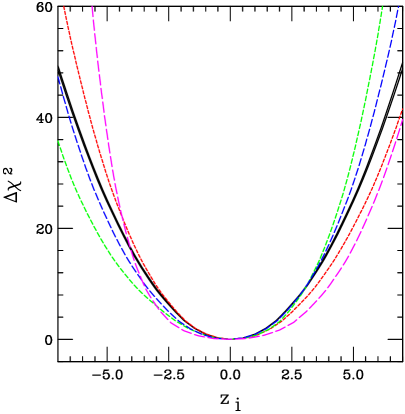
Figure 9: Variation of $\chi^{2}$ with distance along representative eigenvector directions $1$, $4$, $7$, $10$, $13$, $16$. The first two, shown by solid curves, are nearly indistinguishable from each other and from the ideal $\Delta\chi^{2}=z^{2}$. The remaining four, shown by dashed curves with increasing dash length denoting increasing eigenvector number, demonstrate that the quadratic approximation is adequate, though imperfect.

Figure 10

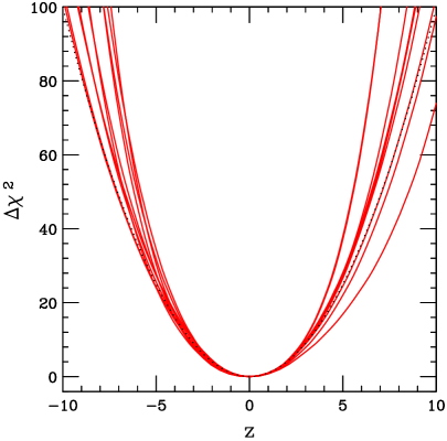
Figure 10: Variation of $\chi^{2}$ with distance along 10 randomly chosen directions in $\{z_{i}\}$ space. The dependence is represented acceptably well by the quadratic approximation $\Delta\chi^{2}=z^{2}$, which is shown as the dotted curve.

shows the dependence of $\chi^{2}$ along some random directions in $\{z_{i}\}$ space. The behavior is reasonably close to the ideal quadratic curve $\Delta\chi^{2}=z^{2}$, implying that the quadratic approximation (7) is adequate. In particular, the approximation gives the range of $z$ permitted by $T=10$ to an accuracy of $\approx\!30\%$. Since the tolerance parameter $T$ used to make the uncertainty estimates is known only to perhaps $50\%$, this level of accuracy is sufficient.

Appendix C Table of Best Fit $S_{0}$

Table 3 lists the parameter values that define the “best fit” PDF set $S_{0}$ which minimizes $\chi_{\mathrm{global}}^{2}$. It also lists the uncertainties (for $T=5$) in those parameters.

For each of the $d\!=\!16$ parameters, Table 3 also lists the components of a unit vector $z_{1},\ldots,z_{d}$ in the eigenvector basis. That unit vector gives the direction for which the parameter varies most rapidly with $\chi_{\mathrm{global}}^{2}$, i.e., the direction along which the parameter reaches its extreme values for a given increase in $\chi_{\mathrm{global}}^{2}$. For parameter $a_{i}$, the components $z_{k}$ are proportional to $M_{ik}$ according to Eq. (29).

Parameter	Value	Error	$z_{1}$	$z_{2}$	$z_{3}$	$z_{4}$	$z_{5}$	$z_{6}$	$z_{7}$	$z_{8}$
			$z_{9}$	$z_{10}$	$z_{11}$	$z_{12}$	$z_{13}$	$z_{14}$	$z_{15}$	$z_{16}$
$A_{1}^{u_{v}}+1$	$0.466$	$.094$	$.04$	$-.01$	$.00$	$-.08$	$-.04$	$-.09$	$.05$	$.07$
		$+.083\,-.079$	$-.06$	$-.06$	$.35$	$-.74$	$-.37$	$-.39$	$-.06$	$.00$
$A_{2}^{u_{v}}$	$3.360$	$.122$	$-.01$	$-.01$	$.03$	$-.14$	$-.07$	$-.37$	$-.32$	$.46$
		$+.112\,-.106$	$.54$	$-.13$	$.06$	$-.23$	$.17$	$.09$	$.35$	$.04$
$\ln(1+A_{3}^{u_{v}})$	$2.553$	$0.51$	$.00$	$.00$	$.00$	$.00$	$.06$	$-.01$	$-.06$	$-.07$
		$+.44\,-.45$	$.10$	$.02$	$-.36$	$.73$	$.36$	$.41$	$.13$	$.03$
$A_{4}^{u_{v}}$	$0.855$	$.118$	$.01$	$.00$	$-.04$	$.19$	$-.09$	$-.13$	$-.29$	$.51$
		$+.110\,-.118$	$.48$	$-.05$	$.05$	$.06$	$.47$	$.19$	$.30$	$-.01$
$A_{2}^{d_{v}}$	$4.230$	$.45$	$.00$	$.00$	$.00$	$.00$	$.06$	$-.06$	$.00$	$.02$
		$+.45\,-.40$	$-.05$	$.13$	$.72$	$.45$	$.32$	$-.23$	$-.30$	$.08$
$\ln(1+A_{3}^{d_{v}})$	$2.388$	$0.64$	$.00$	$.00$	$.00$	$.00$	$-.04$	$.00$	$.04$	$.05$
		$+.59\,-.62$	$-.08$	$.05$	$-.04$	$.88$	$.38$	$.26$	$-.03$	$.06$
$A_{4}^{d_{v}}$	$0.763$	$0.30$	$.00$	$.00$	$.00$	$-.01$	$-.06$	$.16$	$-.13$	$-.18$
		$+.24\,-.23$	$.26$	$.11$	$.52$	$.37$	$.49$	$-.11$	$-.41$	$.08$
$\ln{\widetilde{f_{g}}}$	$-1.047$	$.018$	$.01$	$.79$	$.32$	$.12$	$.19$	$-.25$	$-.16$	$.09$
		$+.018\,-.019$	$-.19$	$.26$	$.00$	$-.05$	$-.03$	$.00$	$-.06$	$-.11$
$A_{1}^{g}+1$	$0.469$	$0.40$	$.00$	$.00$	$.02$	$.01$	$.02$	$.02$	$.23$	$.05$
		$+0.39\,-0.35$	$.22$	$.29$	$.00$	$.03$	$-.09$	$.04$	$.12$	$.89$
$A_{2}^{g}$	$5.574$	$2.65$	$.00$	$.00$	$.00$	$.00$	$.00$	$.00$	$.00$	$.00$
		$+2.98\,-2.30$	$.00$	$-.03$	$.01$	$.01$	$-.03$	$.03$	$.11$	$.99$
$A_{1}^{\bar{d}+\bar{u}}+1$	$-.009$	$.148$	$.00$	$-.03$	$.10$	$.07$	$.01$	$.01$	$-.24$	$-.07$
		$+.142\,-.119$	$-.15$	$-.65$	$.06$	$.15$	$-.13$	$-.07$	$-.09$	$-.65$
$A_{2}^{\bar{d}+\bar{u}}$	$7.866$	$0.96$	$.00$	$.00$	$.00$	$.00$	$.00$	$.00$	$.04$	$.00$
		$+1.05\,-1.09$	$.01$	$-.21$	$.03$	$-.15$	$.89$	$.28$	$-.10$	$-.22$
$\ln(1+A_{3}^{\bar{d}+\bar{u}})$	$2.031$	$0.89$	$.00$	$.00$	$.00$	$.00$	$.00$	$.00$	$-.03$	$.00$
		$+.78\,-.89$	$-.04$	$.29$	$-.05$	$-.28$	$.66$	$.20$	$.04$	$.59$
$\ln B_{0}^{\bar{d}/\bar{u}}$	$10.29$	$1.45$	$.00$	$.00$	$.00$	$.00$	$-.01$	$-.02$	$.01$	$-.04$
		$+1.551\,-1.496$	$.00$	$.01$	$.03$	$.00$	$.00$	$.06$	$.94$	$-.32$
$B_{1}^{\bar{d}/\bar{u}}$	$5.379$	$0.85$	$.00$	$.00$	$.00$	$-.01$	$.02$	$.06$	$-.02$	$.10$
		$+1.02\,-.75$	$-.02$	$-.03$	$.01$	$.04$	$.16$	$-.21$	$.93$	$-.24$
$B_{4}^{\bar{d}/\bar{u}}$	$4.498$	$1.21$	$.00$	$.00$	$.00$	$.00$	$.00$	$.01$	$.00$	$.01$
		$+1.20\,-1.12$	$.00$	$.01$	$.06$	$-.04$	$-.27$	$.94$	$-.01$	$-.20$

Table 3: Parameters of the global fit. Errors shown are for $T\!=\!5$, i.e., $\Delta\chi_{\rm global}^{2}=25$. Fixed parameters: $A_{4}^{\bar{d}+\bar{u}}\!=\!1.0$, $B_{2}^{\bar{d}/\bar{u}}\!=\!15.0$, $B_{3}^{\bar{d}/\bar{u}}\!=\!10.0$, and $A_{3}^{g}\!=\!0.0\,\Rightarrow\,A_{4}^{g}\,{\rm irrelevant}$. The $z_{k}$ are proportional to the $z_{k}(a_{i}^{\pm})=\pm\,t\,M_{ik}$ of Eq. (29) and are normalized to $\sum_{k}z_{k}^{2}=1$.

Appendix D Table and Graphs of the Eigenvector sets $S_{\ell}^{\pm}$

$-0.1941$	$-0.5337$	$3.3604$	$11.8404$	$0.8552$	$\ln A_{0}^{u_{v}}$	$A_{1}^{u_{v}}$	$A_{2}^{u_{v}}$	$A_{3}^{u_{v}}$	$A_{4}^{u_{v}}$
$-0.7175$	$-0.5337$	$4.2296$	$9.8950$	$0.7628$	$\ln A_{0}^{d_{v}}$	$A_{1}^{d_{v}}$	$A_{2}^{d_{v}}$	$A_{3}^{d_{v}}$	$A_{4}^{d_{v}}$
$1.8914$	$-0.5305$	$5.5737$	$0.0000$	$1.0000$	$\ln A_{0}^{g}$	$A_{1}^{g}$	$A_{2}^{g}$	$A_{3}^{g}$	$A_{4}^{g}$
$-1.1174$	$-1.0092$	$7.8658$	$6.6187$	$1.0000$	$\ln A_{0}^{\bar{d}+\bar{u}}$	$A_{1}^{\bar{d}+\bar{u}}$	$A_{2}^{\bar{d}+\bar{u}}$	$A_{3}^{\bar{d}+\bar{u}}$	$A_{4}^{\bar{d}+\bar{u}}$
$10.2940$	$5.3793$	$15.0000$	$10.0000$	$4.4980$	$\ln B_{0}^{\bar{d}/\bar{u}}$	$B_{1}^{\bar{d}/\bar{u}}$	$B_{2}^{\bar{d}/\bar{u}}$	$B_{3}^{\bar{d}/\bar{u}}$	$B_{4}^{\bar{d}/\bar{u}}$
$-0.1841$	$-0.5298$	$3.3596$	$11.8478$	$0.8558$	$-0.2042$	$-0.5376$	$3.3612$	$11.8331$	$0.8546$
$-0.7064$	$-0.5298$	$4.2295$	$9.8957$	$0.7629$	$-0.7285$	$-0.5376$	$4.2297$	$9.8942$	$0.7627$
$1.8919$	$-0.5304$	$5.5737$	$0.0000$	$1.0000$	$1.8910$	$-0.5306$	$5.5737$	$0.0000$	$1.0000$
$-1.1342$	$-1.0089$	$7.8658$	$6.6191$	$1.0000$	$-1.1010$	$-1.0095$	$7.8658$	$6.6182$	$1.0000$
$10.2940$	$5.3793$	$15.0000$	$10.0000$	$4.4980$	$10.2940$	$5.3793$	$15.0000$	$10.0000$	$4.4980$
$-0.1951$	$-0.5343$	$3.3597$	$11.8372$	$0.8557$	$-0.1931$	$-0.5331$	$3.3611$	$11.8437$	$0.8547$
$-0.7184$	$-0.5343$	$4.2291$	$9.8952$	$0.7636$	$-0.7165$	$-0.5331$	$4.2301$	$9.8947$	$0.7620$
$1.9025$	$-0.5321$	$5.5740$	$0.0000$	$1.0000$	$1.8802$	$-0.5288$	$5.5734$	$0.0000$	$1.0000$
$-1.1609$	$-1.0140$	$7.8662$	$6.6117$	$1.0000$	$-1.0751$	$-1.0043$	$7.8654$	$6.6256$	$1.0000$
$10.2940$	$5.3794$	$15.0000$	$10.0000$	$4.4980$	$10.2940$	$5.3792$	$15.0000$	$10.0000$	$4.4980$
$-0.1981$	$-0.5338$	$3.3645$	$11.8237$	$0.8501$	$-0.1903$	$-0.5336$	$3.3564$	$11.8567$	$0.8602$
$-0.7182$	$-0.5338$	$4.2287$	$9.9098$	$0.7633$	$-0.7167$	$-0.5336$	$4.2304$	$9.8806$	$0.7623$
$1.9095$	$-0.5244$	$5.5730$	$0.0000$	$1.0000$	$1.8738$	$-0.5364$	$5.5745$	$0.0000$	$1.0000$
$-1.0925$	$-0.9946$	$7.8651$	$6.6340$	$1.0000$	$-1.1422$	$-1.0234$	$7.8665$	$6.6037$	$1.0000$
$10.2939$	$5.3795$	$15.0000$	$10.0000$	$4.4980$	$10.2941$	$5.3791$	$15.0000$	$10.0000$	$4.4980$
$-0.1932$	$-0.5413$	$3.3436$	$11.8275$	$0.8774$	$-0.1960$	$-0.5260$	$3.3774$	$11.8536$	$0.8327$
$-0.7420$	$-0.5413$	$4.2312$	$9.8814$	$0.7592$	$-0.6928$	$-0.5260$	$4.2279$	$9.9087$	$0.7664$
$1.9005$	$-0.5271$	$5.5735$	$0.0000$	$1.0000$	$1.8822$	$-0.5340$	$5.5739$	$0.0000$	$1.0000$
$-1.0798$	$-0.9990$	$7.8655$	$6.6250$	$1.0000$	$-1.1544$	$-1.0195$	$7.8661$	$6.6122$	$1.0000$
$10.2964$	$5.3748$	$15.0000$	$10.0000$	$4.4970$	$10.2916$	$5.3839$	$15.0000$	$10.0000$	$4.4990$
$-0.2373$	$-0.5372$	$3.3513$	$12.2488$	$0.8440$	$-0.1528$	$-0.5303$	$3.3692$	$11.4555$	$0.8661$
$-0.7278$	$-0.5372$	$4.2550$	$9.5924$	$0.7435$	$-0.7078$	$-0.5303$	$4.2049$	$10.1974$	$0.7816$
$1.9071$	$-0.5244$	$5.5733$	$0.0000$	$1.0000$	$1.8761$	$-0.5364$	$5.5742$	$0.0000$	$1.0000$
$-1.1096$	$-1.0071$	$7.8668$	$6.6099$	$1.0000$	$-1.1246$	$-1.0112$	$7.8648$	$6.6272$	$1.0000$
$10.2848$	$5.3943$	$15.0000$	$10.0000$	$4.5012$	$10.3029$	$5.3647$	$15.0000$	$10.0000$	$4.4949$
$-0.2370$	$-0.5419$	$3.3147$	$11.7529$	$0.8399$	$-0.1529$	$-0.5258$	$3.4046$	$11.9257$	$0.8700$
$-0.6899$	$-0.5419$	$4.2039$	$9.8658$	$0.8113$	$-0.7483$	$-0.5258$	$4.2545$	$9.9232$	$0.7159$
$1.9021$	$-0.5228$	$5.5734$	$0.0000$	$1.0000$	$1.8811$	$-0.5379$	$5.5741$	$0.0000$	$1.0000$
$-1.0919$	$-1.0074$	$7.8633$	$6.6099$	$1.0000$	$-1.1398$	$-1.0109$	$7.8682$	$6.6271$	$1.0000$
$10.2670$	$5.4325$	$15.0000$	$10.0000$	$4.5101$	$10.3201$	$5.3279$	$15.0000$	$10.0000$	$4.4863$
$-0.2078$	$-0.5282$	$3.3181$	$11.4087$	$0.8179$	$-0.1833$	$-0.5383$	$3.3960$	$12.2156$	$0.8866$
$-0.7700$	$-0.5282$	$4.2279$	$10.1816$	$0.7198$	$-0.6769$	$-0.5383$	$4.2310$	$9.6594$	$0.7990$
$2.0853$	$-0.4301$	$5.5687$	$0.0000$	$1.0000$	$1.7217$	$-0.6150$	$5.5779$	$0.0000$	$1.0000$
$-1.2032$	$-1.0484$	$7.9025$	$6.3721$	$1.0000$	$-1.0446$	$-0.9762$	$7.8349$	$6.8326$	$1.0000$
$10.3046$	$5.3626$	$15.0000$	$10.0000$	$4.4919$	$10.2850$	$5.3934$	$15.0000$	$10.0000$	$4.5031$
$-0.0801$	$-0.5269$	$3.4174$	$11.3977$	$0.9160$	$-0.3093$	$-0.5402$	$3.3060$	$12.2779$	$0.7971$
$-0.7805$	$-0.5269$	$4.2376$	$10.2241$	$0.7090$	$-0.6640$	$-0.5402$	$4.2220$	$9.5897$	$0.8142$
$1.9359$	$-0.5086$	$5.5686$	$0.0000$	$1.0000$	$1.8485$	$-0.5514$	$5.5786$	$0.0000$	$1.0000$
$-1.1401$	$-1.0195$	$7.8611$	$6.6228$	$1.0000$	$-1.0838$	$-0.9994$	$7.8703$	$6.6147$	$1.0000$
$10.2407$	$5.4629$	$15.0000$	$10.0000$	$4.5154$	$10.3449$	$5.2995$	$15.0000$	$10.0000$	$4.4814$

Table 4: Parameters of the Best Fit $S_{0}$ and their definitions, followed by Eigenvector Sets $S_{1}^{+},S_{1}^{-},S_{2}^{+},S_{2}^{-},\dots$.

$-0.1659$	$-0.5391$	$3.4265$	$12.5012$	$0.9121$	$-0.2243$	$-0.5283$	$3.2943$	$11.2121$	$0.7983$
$-0.6220$	$-0.5391$	$4.2087$	$9.3472$	$0.8414$	$-0.8285$	$-0.5283$	$4.2505$	$10.4716$	$0.6842$
$2.0550$	$-0.4456$	$5.5690$	$0.0000$	$1.0000$	$1.7218$	$-0.6154$	$5.5785$	$0.0000$	$1.0000$
$-1.1277$	$-1.0312$	$7.8798$	$6.3693$	$1.0000$	$-1.0969$	$-0.9873$	$7.8518$	$6.8764$	$1.0000$
$10.2997$	$5.3659$	$15.0000$	$10.0000$	$4.4929$	$10.2883$	$5.3927$	$15.0000$	$10.0000$	$4.5031$
$-0.2209$	$-0.5385$	$3.3464$	$11.9679$	$0.8505$	$-0.1581$	$-0.5272$	$3.3793$	$11.6700$	$0.8616$
$-0.7087$	$-0.5385$	$4.2773$	$10.1973$	$0.7903$	$-0.7304$	$-0.5272$	$4.1650$	$9.4988$	$0.7256$
$2.0697$	$-0.4336$	$5.4996$	$0.0000$	$1.0000$	$1.6342$	$-0.6616$	$5.6741$	$0.0000$	$1.0000$
$-1.4530$	$-1.0911$	$7.6927$	$8.5071$	$1.0000$	$-0.6805$	$-0.8983$	$8.1000$	$4.6459$	$1.0000$
$10.3080$	$5.3568$	$15.0000$	$10.0000$	$4.5032$	$10.2750$	$5.4097$	$15.0000$	$10.0000$	$4.4910$
$0.0212$	$-0.4998$	$3.3685$	$9.5867$	$0.8619$	$-0.3963$	$-0.5645$	$3.3530$	$14.3021$	$0.8491$
$-0.3803$	$-0.4998$	$4.5680$	$9.5749$	$0.9267$	$-1.0637$	$-0.5645$	$3.9221$	$10.1942$	$0.6138$
$1.8986$	$-0.5295$	$5.5981$	$0.0000$	$1.0000$	$1.8849$	$-0.5314$	$5.5516$	$0.0000$	$1.0000$
$-1.0511$	$-0.9997$	$7.8935$	$6.2437$	$1.0000$	$-1.1519$	$-1.0178$	$7.8406$	$6.9762$	$1.0000$
$10.3431$	$5.3894$	$15.0000$	$10.0000$	$4.5718$	$10.2494$	$5.3702$	$15.0000$	$10.0000$	$4.4309$
$-0.6200$	$-0.6029$	$3.3322$	$17.6542$	$0.8617$	$0.2128$	$-0.4640$	$3.3889$	$7.8121$	$0.8487$
$-1.0990$	$-0.6029$	$4.4299$	$18.0058$	$0.8742$	$-0.3418$	$-0.4640$	$4.0277$	$5.2176$	$0.6505$
$1.9215$	$-0.5171$	$5.5927$	$0.0000$	$1.0000$	$1.8610$	$-0.5440$	$5.5546$	$0.0000$	$1.0000$
$-0.9608$	$-0.9876$	$7.7202$	$4.9575$	$1.0000$	$-1.2706$	$-1.0310$	$8.0126$	$8.7623$	$1.0000$
$10.2885$	$5.4121$	$15.0000$	$10.0000$	$4.4446$	$10.2995$	$5.3462$	$15.0000$	$10.0000$	$4.5518$
$-0.3285$	$-0.5667$	$3.3800$	$14.2366$	$0.9075$	$-0.0441$	$-0.4965$	$3.3383$	$9.5883$	$0.7962$
$-0.7740$	$-0.5667$	$4.3664$	$12.6923$	$0.9007$	$-0.6624$	$-0.4965$	$4.0754$	$7.4209$	$0.6073$
$1.8124$	$-0.5621$	$5.5060$	$0.0000$	$1.0000$	$1.9800$	$-0.4949$	$5.6501$	$0.0000$	$1.0000$
$-1.3022$	$-1.0266$	$8.6732$	$12.2662$	$1.0000$	$-0.9707$	$-0.9896$	$6.9557$	$3.0774$	$1.0000$
$10.2946$	$5.5039$	$15.0000$	$10.0000$	$4.1962$	$10.2934$	$5.2389$	$15.0000$	$10.0000$	$4.8382$
$-0.4030$	$-0.5716$	$3.3718$	$14.9177$	$0.8788$	$-0.0012$	$-0.4980$	$3.3497$	$9.4869$	$0.8330$
$-0.9934$	$-0.5716$	$4.1229$	$11.9127$	$0.7280$	$-0.4696$	$-0.4980$	$4.3301$	$8.2828$	$0.7956$
$1.9461$	$-0.5128$	$5.6623$	$0.0000$	$1.0000$	$1.8398$	$-0.5471$	$5.4902$	$0.0000$	$1.0000$
$-1.1804$	$-1.0206$	$8.1430$	$8.1232$	$1.0000$	$-1.0571$	$-0.9985$	$7.6046$	$5.4285$	$1.0000$
$10.3763$	$5.1976$	$15.0000$	$10.0000$	$5.6698$	$10.2164$	$5.5506$	$15.0000$	$10.0000$	$3.3936$
$-0.2036$	$-0.5399$	$3.4062$	$12.7490$	$0.8931$	$-0.1860$	$-0.5282$	$3.3199$	$11.0884$	$0.8217$
$-0.9051$	$-0.5399$	$4.0867$	$9.6572$	$0.6340$	$-0.5709$	$-0.5282$	$4.3557$	$10.1093$	$0.8765$
$2.0530$	$-0.4819$	$5.8758$	$0.0000$	$1.0000$	$1.7480$	$-0.5734$	$5.3071$	$0.0000$	$1.0000$
$-1.1784$	$-1.0238$	$7.7670$	$6.9327$	$1.0000$	$-1.0517$	$-0.9963$	$7.9530$	$6.3518$	$1.0000$
$11.7435$	$6.2127$	$15.0000$	$10.0000$	$4.4913$	$9.0144$	$4.6435$	$15.0000$	$10.0000$	$4.5039$
$-0.2054$	$-0.5338$	$3.3661$	$12.0453$	$0.8534$	$-0.1853$	$-0.5336$	$3.3560$	$11.6819$	$0.8566$
$-0.7110$	$-0.5338$	$4.2688$	$10.4095$	$0.7879$	$-0.7226$	$-0.5336$	$4.1988$	$9.5075$	$0.7431$
$3.2798$	$-0.1380$	$8.5257$	$0.0000$	$1.0000$	$0.7313$	$-0.8385$	$3.2571$	$0.0000$	$1.0000$
$-1.7279$	$-1.1163$	$7.6289$	$12.7489$	$1.0000$	$-0.6889$	$-0.9252$	$8.0517$	$3.7937$	$1.0000$
$9.7697$	$5.1479$	$15.0000$	$10.0000$	$4.2287$	$10.7054$	$5.5609$	$15.0000$	$10.0000$	$4.7094$

Table 5: Continuation of Table 4: parameters of the Eigenvector Sets $S_{9}^{+},S_{9}^{-}$, …, $S_{16}^{+},S_{16}^{-}$.

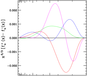
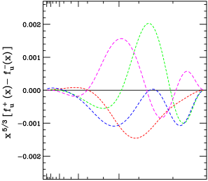
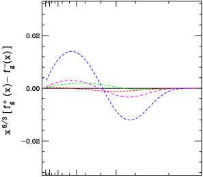
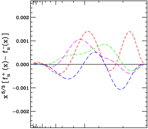
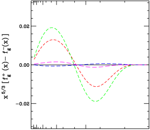
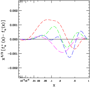
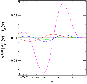
Figure 11: Displacements of the $u$-quark and gluon distributions $f^{+}(x,Q)\!-\!f^{-}(x,Q)$ at $Q=10\,{\rm GeV}$ corresponding to $S^{+}_{\ell}\!-\!S^{-}_{\ell}$. Length of dashes increases for $\ell=1,\ldots,16$.

Table 4 and its continuation Table 5 completely specify the PDF Eigenvector Basis sets $S^{+}_{\ell}$ and $S^{-}_{\ell}$ by listing all of their parameters at $Q_{0}$. The notation and the best-fit set $\,S_{0}$ are specified at the beginning of the table.

The coefficients listed provide all of the information that is needed for applications. For completeness, however, we state here explicitly the connections between these coefficients and the constructs that were used elsewhere in the paper to derive them. The fit parameters $\{a_{i}\}$ are related to the tabulated parameters by

$$\begin{array}[]{llll}a_{1}=A_{1}^{u_{v}}+1,&a_{2}=A_{2}^{u_{v}},&a_{3}=\ln(1+A_{3}^{u_{v}}),&a_{4}=A_{4}^{u_{v}},\\ a_{5}=A_{2}^{d_{v}},&a_{6}=\ln(1+A_{3}^{d_{v}}),&a_{7}=A_{4}^{d_{v}},&a_{8}=\ln{\widetilde{f_{g}}},\\ a_{9}=A_{1}^{g}+1,&a_{10}=A_{2}^{g},&a_{11}=A_{1}^{\,\bar{d}+\bar{u}}+1,&a_{12}=A_{2}^{\,\bar{d}+\bar{u}},\\ a_{13}=\ln(1+A_{3}^{\bar{d}+\bar{u}}),&a_{14}=\ln B_{0}^{\bar{d}/\bar{u}},&a_{15}=B_{1}^{\,\bar{d}/\bar{u}},&a_{16}=B_{4}^{\,\bar{d}/\bar{u}}\end{array}\;.$$ (33)

Each of the $a_{i}$ is thus related to a single PDF parameter, except for $a_{8}$ which is related to $\widetilde{f_{g}}$, the momentum fraction carried by gluons, and is thus determined by $A_{0}^{g},\ldots,A_{4}^{g}$. The matrix elements of the transformation from the $a_{i}$ coordinates to the eigenvector coordinates are given by

$$M_{i\ell}=\frac{a_{i}(S^{+}_{\ell})-a_{i}(S^{-}_{\ell})}{2\,t}$$ (34)

according to (18), where $t=5$ because that value was used to generate the $S_{\ell}^{\pm}$. Eqs. (9) and (14) imply

$$\sum_{i=1}^{d}\,M_{i\ell}\,M_{ik}=s_{\ell}\,s_{k}\,\delta_{\ell k}\;.$$ (35)

For $\ell\neq k$, this becomes $\sum_{i=1}^{d}M_{i\ell}M_{ik}=0$, which can serve as a check on numerical accuracy; while for $\ell=k$, it becomes $\sum_{i=1}^{d}M_{i\ell}^{\,2}=s_{\ell}^{\,2}$ which can be used to reconstruct $s_{1},\ldots,s_{d}$.

Finally, for the benefit of the reader who is curious about them, graphs are shown in Fig. 11 of the differences described by each of the PDF eigenvector sets. One sees that the steeper directions (small values of $\ell$) mainly control aspects of the quark distribution, while the shallower directions (high values of $\ell$) control the gluon distribution, whose absolute uncertainty is larger. The variations in the gluon distribution show less variety than the quarks because the gluon distribution is described by only $3$ parameters (including normalization), such that the most general variation for it is of the form $\frac{\Delta g}{g}=c_{1}+c_{2}\log x+c_{3}\log(1-x)$.

References

- [1] H. L. Lai, J. Huston, S. Kuhlmann, J. Morfin, F. Olness, J. F. Owens, J. Pumplin and W. K. Tung, Eur. Phys. J. C12, 375 (2000) [hep-ph/9903282].
- [2] A. D. Martin, R. G. Roberts, W. J. Stirling, and R. S. Thorne, Eur. Phys. J. C4, 463 (1998) [hep-ph/9803445].
- [3] M. Gluck, E. Reya and A. Vogt, Eur. Phys. J. C5, 461 (1998) [hep-ph/9806404].
- [4] James Botts, et al., Phys. Lett. B304, 159 (1993); H. L. Lai, et al., Phys. Rev. D51, 4763 (1995); H. L. Lai, et al., Phys. Rev. D55, 1280 (1997).
- [5] A. D. Martin, R. G. Roberts, W. J. Stirling, and R. S. Thorne, Eur. Phys. J., C14, 133 (2000) [hep-ph/9907231].
- [6] J. Huston, S. Kuhlmann, H. L. Lai, F. Olness, J. F. Owens, D. E. Soper and W. K. Tung, Phys. Rev. D58, 114034 (1998) [hep-ph/9801444].
- [7] Contributions to the Proceedings of the Workshop QCD and Weak Boson Physics in Run II, Fermilab-Pub-00/297 (U. Baur, R. K. Ellis, and D. Zeppenfeld, eds.) to be published.
- [8] S. Catani et al., The QCD and standard model working group: Summary report, LHC Workshop Standard Model and More, CERN, 1999 [hep-ph/0005114].
- [9] S. Alekhin, Eur. Phys. J. C10, 395 (1999) [hep-ph/9611213]; contribution to Proceedings of Standard Model Physics (and more) at the LHC, [8]; and S. I. Alekhin, [hep-ph/0011002].
- [10] M. Botje, Eur. Phys. J. C14, 285 (2000) [hep-ph/9912439].
- [11] V. Barone, C. Pascaud, and F. Zomer, Eur. Phys. J. C12, 243 (2000) [hep-ph/9907512]; C. Pascaud and F. Zomer, LAL-95-05.
- [12] W. T. Giele and S. Keller, Phys. Rev. D58, 094023 (1998) [hep-ph/9803393]; D. Kosower, talk given at ‘Les Rencontres de Physique de la Vall e d’Aoste’, La Thuile, February 1999; W. T. Giele, S. Keller and D. Kosower, in Ref. [7].
- [13] R. Brock, D. Casey, J. Huston, J. Kalk, J. Pumplin, D. Stump, W. K. Tung, in Ref. [7].
- [14] W. Bialek, C.G. Callan, S.P. Strong, Phys. Rev. Lett. 77, 4693 (1996); V. Periwal, Phys. Rev. D59, 094006 (1999).
- [15] R.D. Ball in the proceedings of the XXXIVth Rencontres de Moriond, “QCD and Hadronic Interactions”, Les Arcs, March 1999.
- [16] Particle Data Group, Eur. Phys. J. C15, 1 (2000).
- [17] J. Pumplin, D.R. Stump, and W.K. Tung, Multivariate fitting and the error matrix in global analysis of data, Submitted to Phys. Rev. D [hep-ph/0008191].
- [18] D. Stump, J. Pumplin, R. Brock, D. Casey, J. Huston, J. Kalk, W.-K. Tung, “Uncertainties of predictions from parton distribution functions I: the Lagrange Multiplier method” [hep-ph/0101051].
- [19] BCDMS Collaboration (A.C. Benvenuti, et.al..), Phys.Lett. B223, 485 (1989); and Phys. Lett.B237, 592 (1990).
- [20] H1 Collaboration (S. Aid et al.): “1993 data” Nucl. Phys. B439, 471 (1995); “1994 data”, DESY-96-039, [hep-ex/9603004] and H1 Webpage.
- [21] ZEUS Collaboration (M. Derrick et al.): “1993 data” Z. Phys. C65, 379 (1995) ; “1994 data”, DESY-96-076 (1996).
- [22] NMC Collaboration: (M. Arneodo et al.) Phys. Lett. B364, 107 (1995).
- [23] CCFR Collaboration (W.C. Leung, et al.), Phys. Lett. B317, 655 (1993); and (P.Z. Quintas, et al.), Phys. Rev. Lett. 71, 1307 (1993).
- [24] E605: (G. Moreno, et al.), Phys. Rev. D43, 2815 (1991).
- [25] NA51 Collaboration (A. Baldit, et al.), Phys. Lett. B332, 244 (1994).
- [26] E866 Collaboration (E.A. Hawker, et al.), Phys. Rev. Lett. 80, 3175 (1998).
- [27] CDF Collaboration (F. Abe, et al.), Phys. Rev. Lett. 74, 850 (1995).
- [28] D0 Collaboration: (B. Abbott et al.), Phys. Rev. Lett. 82, 2451 (1999) [hep-ex/9807018].
- [29] CDF Collaboration (Abe et al.), Phys. Rev. Lett. 77, (1996) 439, and F. Bedeschi, talk at 1999 Hadron Collider Physics Conference, Bombay, January, 1999.
- [30] F. James, M. Roos, Comput. Phys. Commun. 10, 343 (1975); Minuit manual, http://wwwinfo.cern.ch/asdoc/minuit/.
- [31] F. Lehner, “Some aspects of W / Z boson physics at the Tevatron” in Proceedings of 4th Rencontres du Vietnam: International Conference on Physics at Extreme Energies (Particle Physics and Astrophysics), Hanoi, Vietnam, 19-25 Jul 2000, FERMILAB-CONF-00-273-E, Oct 2000.