FZJ-IKP(TH)-2001-01

Complete analysis of pion–nucleon scattering
in chiral perturbation theory to third order

Nadia Fettes, Ulf-G. Meißner

Forschungszentrum Jülich, Institut für Kernphysik (Theorie)

D–52425 Jülich, Germany

We consider pion–nucleon scattering in heavy–baryon chiral perturbation theory to third order. All electromagnetic corrections appearing to this order are included. We thus have a consistent description of strong and electromagnetic effects, which allows us to isolate the strong part of the interaction in an unambiguous way. We give pion–nucleon phase shifts up to pion laboratory momenta of 100 MeV and find sizeable differences for the S–waves of the elastic channels compared to previous phase shift analyses. The precise description of the scattering process also allows us to address the question of isospin violation in the strong interaction. For the usually employed triangle relation we find an isospin breaking effect of $-0.7\%$ in the S–wave, whereas the P–waves show an effect of $-1.5\%$ and $-4$ to $-2.5\%$, respectively, for pion laboratory momenta between 25 and 100 MeV.

PACS: 13.75.Gx, 25.80.Dj, 12.39.Fe

Keywords: Pion–nucleon scattering, chiral perturbation theory, isospin symmetry

1 Introduction

The study of the strong interactions at low energies has stimulated vast efforts in the domain of pion–nucleon physics. It is mainly the description of simple processes like pion–nucleon scattering which can help us to extend our knowledge about the fundamental principles of the strong interactions. For every field theory, the consideration of symmetry principles is very important, and it is thus of primordial interest to know to what extent these symmetries are realized in nature.

For a long time, isospin symmetry has been thought of as an exact symmetry of the strong interactions. But the nucleon isospin doublet, consisting of proton and neutron, is not degenerate in mass; whereas electromagnetic interactions alone would make the proton heavier than the neutron, the mass difference between the up– and down–quarks reverses the situation: the neutron turns out to be heavier than the proton by 1.3 MeV. This simple consideration triggers questions about the size of isospin violation in other strong processes.

Pion–nucleon scattering is the ideal playground for studying the question of isospin breaking. Indeed, thanks to the construction of meson factories and the formidable effort of many experimental groups, we now have a large amount of very precise low–energy data. Weinberg pointed out on purely theoretical grounds that isospin breaking effects in neutral–pion scattering must be dramatically enhanced due to the smallness of the isoscalar amplitudes [2]. The advent of high–quality data opened the way to the study of isospin symmetry violation in processes which are experimentally accessible: these are the elastic $\pi^{+}p$ and $\pi^{-}p$ as well as the single charge exchange (SCX) reactions. The difficulty now lies in the extraction of the strong interaction amplitude from the scattering data. Electromagnetic corrections have to be applied in order to gain information about the hadronic amplitudes. Such corrections have been computed e.g. by the Nordita group [3] and more recently by Gashi et al. [4]. The problem is that these analyses cannot account for the electromagnetic and the strong interaction in a consistent way. In view of studying small quantities like isospin symmetry violation, it is absolutely necessary to avoid systematic errors resulting from a possible mismatch in the description of both forces. We will readdress this question, i.e. we will extract the strong amplitude from scattering data in the framework of chiral perturbation theory ($\chi$PT). $\chi$PT allows to calculate the electromagnetic and the strong interactions consistently in terms of unknown parameters, the so–called low–energy constants (LECs). Having fitted the full amplitude to the available cross section data, one is then able to switch off electromagnetism and to predict the strong piece in a unique fashion.

The knowledge of the hadronic amplitude is necessary for analyzing the violation of isospin symmetry of the strong interaction. Such analyses have been performed in the past [5, 6], indicating breaking at low energies as large as $6\%$. Both works, however, are based on electromagnetic corrections which might not be compatible with the description of the strong interactions. In order to better understand the origin of this large isospin breaking effect, we readdress this question within our framework. The advantage of such a diagrammatic calculation lies in the fact that we can clearly localize which mechanisms are responsible for isospin violation, thus making a detailed study of the subject feasible.

2 The amplitude

This work follows a series of previous papers: in [7], pion–nucleon scattering was studied in the limit of isospin symmetry. The unknown counterterms were determined by a fit to phase shifts resulting from three different analyses [8, 9, 10]. In [11, 12], we included strong isospin breaking terms in the amplitude and took the full mass difference of the physical particles into account. The isospin symmetric amplitude had to be generalized in order to describe scattering of particles with different masses. Not only do the particles in the initial and final states have different masses, but pion mass differences also have to be considered in the loops, and the nucleon mass difference plays a role in the intermediate states.

The aim of this work is to describe QCD and QED with unequal up– and down–quark masses ($m_{u}\neq m_{d}$) and non–vanishing electric charge ($e^{2}\neq 0$). We thus have to add loops with virtual photons as well as electromagnetic counterterms. This is the yet missing part in the complete analysis of pion–nucleon scattering. Photons enter the amplitude via four mechanisms, one example of each is shown in fig. 1.

• First, there is the Coulomb potential, which is the exchange of soft photons between the charged pions and the proton. To the accuracy we are working we only have to include the one– and two–photon exchange, since multi–photon exchange diagrams are suppressed by higher powers of $e^{2}$. It is important to note that our simultaneous counting of momenta $q$ and electromagnetic couplings $e$ as small quantities necessarily breaks down at very low energies. To illustrate this, let us compare the Weinberg–Tomozawa term (which in our counting is of first order) and the same process accompanied by the exchange of a photon between the initial or the final particles. At low energies, the loop diagram (which is of third order) is “suppressed” by a factor $e^{2}M_{\pi}/(32|\vec{q}_{\pi}|)$. Thus, for pions of momentum less than $0.5$ MeV, the loop diagram is not suppressed compared to the tree diagram, which clearly contradicts our counting scheme. At very low energies, one would thus have to sum up diagrams with an arbitrary number of photons exchanged between the charged–particle legs. This is commonly done in nucleon–nucleon scattering, where the heavy nucleons can be considered to be non–relativistic at such energies. Fortunately we do not have to worry about these ladder exchange diagrams since they only become important at energies much lower than the experimentally accessible energy range. In our analysis, we will thus stick to the traditional chiral counting, which consists in considering $e$ a quantity of chiral order $q$.

• Second, there are the “usual” loop diagrams with virtual photons, i.e. those which include at least one strong–interaction vertex. Many of these only renormalize the coupling constants.

• Third, we also have to consider Bremsstrahlung processes where a soft photon is emitted from an external particle, but is not detected since its energy is lower than the detector resolution $\Delta E$. The inclusion of this process makes the amplitude infrared finite. We have not performed this calculation analytically, since it is sufficient for the actual computation to combine every $\log(m_{\gamma}/M_{\pi})$ from virtual–photon diagrams with $\log(\Delta E/m_{\gamma})$ due to the integrated emission of soft photons with energy smaller than the detector resolution. The divergence appearing because of the vanishing photon mass $m_{\gamma}$ thus cancels out. For the evaluation, we choose $\Delta E=10$ MeV.

• Fourth, hard photons have been integrated out of the theory. Their effect is parameterized by a string of terms in the Lagrangian, each accompanied by an unknown coupling constant. These constants, similarly to the hadronic counterterms, have to be fitted to experimental data.

Figure 1: Example diagrams for a) the Coulomb potential, b) a “usual” photon loop, c) Bremsstrahlung, and d) an electromagnetic counterterm. The solid, dashed, and wiggly lines denote nucleons, pions, and photons, in order.

The inclusion of photons and electromagnetic counterterms in the amplitude gives us a description of pion–nucleon scattering based on full QCD and QED. Lepton loops, e.g. vacuum polarization, have not been taken into account explicitly, but their effect is hidden in the electromagnetic counterterms. One could equally well compute lepton loops by using a Lagrangian containing photons and leptons as active degrees of freedom [13], but for our purposes the parameterization of these effects by counterterms is sufficient. Let us add a last remark about the relativistic form of our amplitude. The pions and photons are treated fully relativistically; on the other hand, since we restrict ourselves to the energy region just above threshold, we can consider the nucleons to be very heavy and work in heavy–baryon chiral perturbation theory [14, 15]. This is a particular non–relativistic expansion of the amplitude, which amounts to organizing observables in a series of terms with increasing power of the inverse (heavy–) nucleon mass.

Our calculations are based on the Lagrangian constructed in [16] (see also [17]). The relevant terms can be found in appendix A.

3 Fitting procedure

After having constructed the full amplitude, we can proceed to fixing the unknown parameters. For this we use cross section data for elastic $\pi^{+}p$ and $\pi^{-}p$ scattering as well as for the charge exchange $\pi^{-}p\to\pi^{0}n$ reaction. Guided by the results of [7], we decide to use experimental information up to pion laboratory momenta of $100$ MeV (i.e. $T_{\pi}\leq 32.2$ MeV) as input. We perform a combined fit of our isospin breaking amplitude to all three channels which have been studied experimentally. In the elastic channels, we use the data by Frank et al. [18], Brack et al. [19], and by Joram et al. [20]. Low–energetic charge exchange data have been taken by Isenhower et al. [21], Salomon et al. [22], and by Frlez et al. [23]. Note that we do not include the old data by Bertin et al. [24] and by Duclos et al. [25] in our data base, since these are nowadays generally believed to be erroneous.

In the full amplitude, there appear 14 combinations of parameters which have to be fixed. Such a large number of unknowns makes a determination from pion–nucleon scattering data alone (almost) impossible. But, fortunately, some of these counterterms appear in other processes, which have been studied in great detail. The counterterms $c_{6/7}$, $d_{6/7}$, related to the coupling of a photon to the nucleon, can be fitted to the magnetic moments and the charge radii of proton and neutron (see e.g. [26]). The separation of the nucleon mass difference into a strong and an electromagnetic piece [27, 28] fixes $c_{5}$ and $f_{2}$. We are now left with 11 parameters which have to be determined.

We define the function which has to be minimized in analogy to the one introduced in [29], i.e.

$$\chi^{2}=\sum_{j}w_{j}\chi_{j}^{2}~{},$$ (1)

with

$$\chi_{j}^{2}=\sum_{i=1}^{n_{j}}\frac{(y_{ij}^{\exp}-y_{ij}^{\rm th})^{2}}{(\sigma_{ij}^{\rm stat})^{2}}~{},$$ (2)

the partial contribution of the $j$th data set comprising $n_{j}$ entries, and the weights $w_{j}$ being given by

$$w_{j}=N(\sigma_{j}^{\rm sys})^{-2}/\sum_{j}(\sigma_{j}^{\rm sys})^{-2}~{}.$$ (3)

Here $N$ is the number of data sets we fit to, and the uncertainties are split into a statistical piece $\sigma_{ij}^{\rm stat}$ and a systematic contribution $\sigma_{j}^{\rm sys}$ . The experimental data are denoted by $y_{ij}^{\exp}$, and we choose the LECs in such a way that our predicted cross sections $y_{ij}^{\rm th}$ minimize the $\chi^{2}$–function.

We use the standard MINUIT minimization routines of the CERN library. Table 1 gives our best–fit values at the scale $\lambda=M_{\pi^{0}}$. Note that the quoted errors correspond to the MINUIT errors only and are certainly underestimated. The hadronic low–energy constants are of natural size, i.e. of order 1; as for the electromagnetic counterterms, some come out unnaturally large, but in this case they are accompanied by big uncertainties. It is obvious that one has to be careful about correlated parameters in a fit involving such a large number of unknowns; we indeed have large correlations among the strong–interaction counterterms. This does not come as a surprise since we restrict our analysis to a small energy region above threshold. There the pion energy, for example, is hardly distinguishable from the pion mass which causes the parameters accompanying these two structures to be strongly correlated. For these reasons we refrain from making predictions for quantities like the sigma term or the pion–nucleon coupling constant $g_{\pi NN}$ which are determined by LEC combinations strongly correlated to other parameters. We have checked, however, that there are very small correlations between electromagnetic and strong counterterms. This guarantees that we can reliably extract the strong phases from the full amplitude. The smallness of the $\chi^{2}$/dof value shows that we fit to data in a region where the third order amplitude is still precise enough. More important, it also demonstrates the consistency of the low–energy data base.

LEC
$\tilde{c}_{1}=c_{1}+e^{2}F_{\pi}^{2}f_{1}/(2M_{\pi^{0}}^{2})$	$(0.64\pm 0.04)$ GeV-1
$c_{2}$	$(5.54\pm 0.05)$ GeV-1
$c_{3}$	$(-5.34\pm 0.04)$ GeV-1
$c_{4}$	$(2.84\pm 0.15)$ GeV-1
$\bar{d}_{1}+\bar{d}_{2}$	$(-2.24\pm 0.16)$ GeV-2
$\bar{d}_{3}$	$(0.81\pm 0.16)$ GeV-2
$\bar{d}_{5}$	$(0.67\pm 0.11)$ GeV-2
$\bar{d}_{14}-\bar{d}_{15}$	$(-0.63\pm 0.75)$ GeV-2
$\bar{d}_{18}$	$(-10.14\pm 0.45)$ GeV-2
$\tilde{g}_{6}=\bar{g}_{6}+\bar{g}_{8}-\bar{k}_{8}/(128\pi^{2}F_{\pi}^{2})-\bar{\ell}_{6}/(96\pi^{2}F_{\pi}^{2})$	$(49.48\pm 10.15)$ GeV-2
$\tilde{g}_{7}=\bar{g}_{7}+\bar{k}_{8}/(64\pi^{2}F_{\pi}^{2})$	$(55.07\pm 39.97)$ GeV-2
$f_{2}$	$-0.97$ GeV-1*
$B_{0}(m_{u}-m_{d})c_{5}$	$0.00051$ GeV-1*
$c_{6}$	$5.64$*
$c_{7}$	$-2.88$*
$\bar{d}_{6}$	$0.38$ GeV-2*
$\bar{d}_{7}$	$-0.65$ GeV-2*
$\chi^{2}$/dof	$1.50$

Table 1: Values of the LECs resulting from a fit of the full pion–nucleon amplitude to low–energy cross section data. Parameter values marked by a * are input quantities.

4 Extraction of the strong amplitude

After having determined all low–energy constants appearing in the pion–nucleon amplitude, we can now proceed to extracting the strong interaction piece. As pointed out in the introduction, it is this piece which is of particular interest for the determination of isospin breaking. In the previous paragraph we have used the full amplitude in order to describe pion–nucleon cross sections. The strong amplitude is defined as the QCD scattering amplitude with $m_{u}\neq m_{d}$, but $e^{2}=0$. We will thus not work in the isospin symmetry limit, but we will leave room for strong isospin breaking.

In order to determine the strong amplitude, we have to know what the hadronic masses of the scattering particles are. We can write the charged and neutral pion masses as

$$M_{\pi^{+}}^{2}=M_{0}^{2}\!\!\!\! +\frac{2}{F_{\pi}^{2}}e^{2}C\!\!\!\! +{\cal A}_{+}^{(4)}e^{4}+{\cal B}_{+}^{(4)}e^{2}(m_{u}-m_{d})+{\cal C}_{+}^{(4)}(m_{u}-m_{d})^{2}~{},$$ (4)

$$M_{\pi^{0}}^{2}=M_{0}^{2}\!\!\!\! +{\cal A}_{0}^{(4)}e^{4}+{\cal B}_{0}^{(4)}e^{2}(m_{u}-m_{d})+{\cal C}_{0}^{(4)}(m_{u}-m_{d})^{2}~{}.$$ (5)

Here $M_{0}$ is the bare pion mass (more precisely, the leading term in the quark mass expansion of the pion mass in the two–flavor case with $m_{s}$ fixed), and the ${\cal A}_{+/0}^{(4)}$, ${\cal B}_{+/0}^{(4)}$ and ${\cal C}_{+/0}^{(4)}$ are combinations of low–energy constants from the fourth order mesonic Lagrangian with virtual photons. Note that the pion mass difference to leading order is of purely electromagnetic origin. We obtain the hadronic pion masses by switching off the electromagnetic interaction and using

$$|M_{\pi^{0}}^{h}-M_{\pi^{0}}| \leq 1~{}{\rm MeV}~{},$$ (6)

$$M_{\pi^{+}}^{h} = M_{\pi^{0}}^{h}+0.1~{}{\rm MeV}~{}.$$ (7)

These numbers are based on the work by Knecht and Urech [30] using naturalness of the low–energy constants.

As for the nucleon masses, we have

$$m_{p/n}=m-4M_{\pi^{0}}^{2}c_{1}\mp 2B_{0}(m_{u}-m_{d})c_{5}-e^{2}F_{\pi}^{2}\left(f_{1}+\frac{1\pm 1}{2}f_{2}+f_{3}\right)~{},$$ (8)

in terms of the bare nucleon mass $m$ (i.e. the nucleon mass in the SU(2) chiral limit) and the counterterms given in appendix A. The hadronic masses will then be given by

$$m_{p}^{h} = m-4M_{\pi^{0}}^{2}c_{1}-2B_{0}(m_{u}-m_{d})c_{5}$$ (9)

$$= m_{p}+e^{2}F_{\pi}^{2}(f_{1}+f_{2}+f_{3})~{},$$

$$m_{n}^{h} = m-4M_{\pi^{0}}^{2}c_{1}+2B_{0}(m_{u}-m_{d})c_{5}$$ (10)

$$= m_{n}+e^{2}F_{\pi}^{2}(f_{1}+f_{3})~{}.$$

In the following we will take these mass differences into account, as well for the external particles as for the nucleons and pions in the intermediate states.

It becomes clear from eqs. (9) and (10) that we will not be able to determine the hadronic nucleon masses precisely, since we do not know the value of the LEC combination $(f_{1}+f_{3})$. An additional problem is due to the fact that, after including electromagnetic counterterms into the amplitude, we can no more determine $c_{1}$ and $f_{1}$ separately, as only the combination $\tilde{c}_{1}=c_{1}+e^{2}F_{\pi}^{2}f_{1}/(2M_{\pi^{0}}^{2})$ appears. Since we do not know the precise value of these LECs, all we can do is to assume natural sizes for $f_{1}$ and $f_{3}$; we will thus vary these parameters over the interval $f_{1/3}=(0\pm 1)$ GeV^-1 [12]. Our results will, however, turn out to be insensitive to the precise values of these parameters. Also the lack of knowledge of the absolute value of the hadronic pion masses (see eq. (6)) does not affect our results; only the mass differences are relevant.

Figure 2: Strong pion–nucleon phase shifts as a function of the pion laboratory momentum $q_{\pi}$ for the three measured channels. The solid line corresponds to our solution, the dashed one to the one–sigma uncertainty range. Also shown are the EM98 [9] (stars) and the EM00 [29] (open squares) phases.

Figure 3: Strong pion–nucleon phase shifts as a function of the pion laboratory momentum $q_{\pi}$ for the three measured channels. The solid line corresponds to our solution, the dashed one to the one–sigma uncertainty range. Also shown are the KA85 [8] (full dots) and the SP98 [10] (open diamonds) phases.

Fig. 2 shows our prediction for the strong phases as compared to the phase shift analyses performed by Matsinos et al. [9, 29] which do not contain isospin violating contributions. The range of uncertainty in our prediction, resulting from the correlated error bars of the low–energy constants, is given by the dashed curves. In the P₃–waves, the agreement between both analyses is perfect. In the P₁–waves, our solution is closer to the recent analysis EM00. The most dramatic discrepancy lies in the S–waves of the elastic channels; this difference is not due to the inclusion of the isospin violating effects, but is already present in the isospin symmetric part of the amplitude. The kink in the S–wave phase shift for the charge exchange channel comes from the fact that the ingoing pion needs to have a lab momentum of $\sim 25$ MeV in order to produce the heavier final state. (Remember that only the hadronic mass difference of the involved particles is of relevance.) In fig. 3 we show our solution for the phase shifts compared to the KA85 [8] and the SP98 [10] analyses. The agreement in the P₃–waves is still very good, whereas there are some discrepancies in the P₁ phases. Our $\pi^{+}p$ S–wave phases agree better with the KA85 and SP98 ones than with the EM98(00) solution. But there remains a large difference in the S–wave $\pi^{-}p$ phase shift.

In order to explain where the difference in the S–waves comes from, we further analyze the contributions to the electromagnetic corrections (see fig. 5). The strong phase shifts shown in figs. 2, 3 are obtained when fitting the full pion–nucleon amplitude with virtual photons to the experimental data, and then switching off the electromagnetic coupling. This is also shown by the solid line in fig. 5. The dashed line, on the other hand, is obtained if we do not include all virtual–photon diagrams, but only the one–photon exchange diagram with dressed vertices and the two–photon exchange process (see diagrams a)–c) in fig. 4). The way to treat the one–photon and two–photon exchange between the charged pion and the proton is standard. The inclusion of corrections to the $N\gamma$ and the $\pi\gamma$ vertex does not lead to big changes in the phases. The remaining virtual–loop diagrams (one example of which is drawn in d) in fig. 4) have not been included when drawing the dashed line. We think that such diagrams can only be accounted for correctly when the strong interaction and electromagnetism are treated in a consistent way. These effects are very large and cause this unusual bending of the $\pi^{-}p$ S–wave phase shift. Previous phase shift analyses have obviously underestimated these contributions.

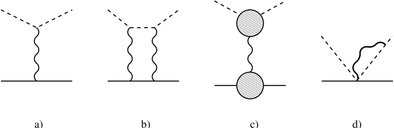
Figure 4: a) One–photon exchange diagram, b) two–photon exchange diagram, c) vertex corrections to the one–photon exchange, d) typical graph involving non–linear pion–nucleon–photon couplings. The solid, dashed, and wiggly lines denote nucleons, pions, and photons, in order

Figure 5: Strong pion–nucleon phase shifts as a function of the pion laboratory momentum $q_{\pi}$. The full line is deduced from an analysis based on the complete pion–nucleon amplitude. To obtain the dashed line, we have fitted the strong amplitude together with the one–photon exchange diagram with dressed vertices and the two–photon exchange process to the data, and then switched off the electromagnetic interaction (see text).

5 Isospin violation of the strong interactions

The aim of this section is to determine the size of isospin violation in low–energy pion–nucleon scattering. Isospin is an approximate symmetry of the strong interactions, for electromagnetism it is largely broken. Consequently, it does not make sense to study isospin violation of the full pion–nucleon amplitude. The interesting part lies in the strong amplitude, which we have isolated in section 4. As in section 4, we will switch off every electromagnetic interaction; we will thus be left with the isospin violating two-pion–nucleon vertex $\sim c_{5}$, and the hadronic mass differences of the nucleons and the pions.

In order to quantify isospin breaking, we will employ the usual triangle ratio [31, 5, 6, 12]

$$R=2\,\frac{f_{\pi^{+}p\to\pi^{+}p}-f_{\pi^{-}p\to\pi^{-}p}-\sqrt{2}\,f_{\pi^{-}p\to\pi^{0}n}}{f_{\pi^{+}p\to\pi^{+}p}-f_{\pi^{-}p\to\pi^{-}p}+\sqrt{2}\,f_{\pi^{-}p\to\pi^{0}n}}~{}.$$ (11)

Here $f$ stands for the strong part of the pion–nucleon amplitude. In the following, we will always form the ratio $R$ with the real part of the scattering amplitude. In case that isospin is a good symmetry $R$ vanishes over the whole energy range.

It has been argued in [12] that it is advantageous not to consider the usual P₃– and P₁–wave projections, but to focus instead on the P–wave parts proportional to the spin–flip and the spin–non–flip amplitudes $h$ and $g$. These are linked to the usual $T$–matrix elements via

$$T_{\pi N} = \sqrt{\frac{E_{1}+m_{1}}{2m_{1}}}\sqrt{\frac{E_{2}+m_{2}}{2m_{2}}}\Big{[}g+i\vec{\sigma}\cdot(\vec{q}_{2}\times\vec{q}_{1}\,)\,h\Big{]}~{}.$$ (12)

$E_{1/2}$ is the energy of the in–/outgoing nucleon with mass $m_{1/2}$, the in–/outgoing pions have four–momenta $q_{1/2}$. The usual S– and P–waves are then given by

$${\rm S}(s) = {{\sqrt{E_{1}+m_{1}}\sqrt{E_{2}+m_{2}}}\over 16\pi\sqrt{s}}{\cal S}(s)~{},$$ (13)

$${\rm P}_{3}(s) = {{\sqrt{E_{1}+m_{1}}\sqrt{E_{2}+m_{2}}}\over 16\pi\sqrt{s}}\,|\vec{q}_{1}||\vec{q}_{2}|\Big{(}{\cal G}(s)+{\cal H}(s)\Big{)}~{},$$ (14)

$${\rm P}_{1}(s) = {{\sqrt{E_{1}+m_{1}}\sqrt{E_{2}+m_{2}}}\over 16\pi\sqrt{s}}\,|\vec{q}_{1}||\vec{q}_{2}|\Big{(}{\cal G}(s)-2{\cal H}(s)\Big{)}~{},$$ (15)

with

$${\cal S}(s) = \int_{-1}^{+1}dz\,g(s,z)~{},$$ (16)

$${\cal G}(s) = \frac{1}{|\vec{q}_{1}||\vec{q}_{2}|}\int_{-1}^{+1}dz\,z\,g(s,z)~{},$$ (17)

$${\cal H}(s) = \int_{-1}^{+1}dz\,\,\frac{z^{2}-1}{2}\,h(s,z)~{}.$$ (18)

The integration in the last equations is performed over the cosine of the scattering angle $z$. In the following we will consider isospin violation in the ${\cal S}$– as well as in the ${\cal G}$– and ${\cal H}$–projections of $R$.

There is one additional problem: as pointed out before, the threshold of the charge exchange reaction lies at $q_{\pi}\sim 25$ MeV. Below this value, the SCX channel is closed and the triangle relation does not make sense. Nevertheless, the different threshold energies of the elastic and the inelastic channels are a consequence of strong isospin breaking (remember that only the hadronic mass difference of the particles has been included). Therefore, we want to take this effect into account; in fig. 6 we show the momentum dependence of $R$ (in $\%$) for momenta $q_{\pi}$ above 25 MeV. In this energy domain all three channels are open. Again, the dashed line indicates the one–sigma uncertainty range of our prediction. For the ${\cal S}$–projection, isospin breaking lies around $-0.7\%$. Also the ${\cal G}$–projection varies very little with energy, breaking in this channel is somewhat larger, $\sim-1.5\%$. The biggest effect is found to be in ${\cal H}$ where isospin violation lies between $-4$ and $-2.5\%$ for $q_{\pi}$ below 100 MeV.

Instead we could also argue that we do not want to take threshold effects into account, and that we want to separate “static” (i.e. related to kinematic effects) from “dynamical” (i.e. due to isospin violating pion–nucleon couplings) isospin breaking [32]. In fig. 7, we consider the case where the hadronic mass of the proton and the neutron, as well as the hadronic mass of the pions, are taken to be equal ($m_{p}^{h}=m_{n}^{h}=(m_{p}+m_{n})/2,M_{\pi^{0}}^{h}=M_{\pi^{+}}^{h}=M_{\pi^{0}}$). There is thus no static isospin breaking, but we only show effects due to the two-pion–nucleon vertex proportional to $c_{5}$. This coupling only shows up in the S–wave of the charge exchange reaction; it causes isospin to be broken by $-0.75\%$ in ${\cal S}$. There is no dynamical isospin breaking in the P–waves (to the order considered here).

Figure 6: $R[\%]$ as a function of the pion laboratory momentum $q_{\pi}$. The dashed lines indicate the one–sigma range of our prediction.

Figure 7: $R[\%]$ as a function of the pion laboratory momentum $q_{\pi}$ in the scenario where $m_{p}^{h}=m_{n}^{h}$ and $M_{\pi^{0}}^{h}=M_{\pi^{+}}^{h}$, as described in the text. The dashed lines indicate the one–sigma range of our prediction.

6 Summary and Outlook

For a reliable determination of the size of isospin breaking in the strong interactions, it is primordial to describe electromagnetic and strong effects consistently. In the present work this is achieved by an analysis of pion–nucleon scattering in the framework of chiral perturbation theory. $\chi$PT does not leave any doubt about the correct definition of the hadronic masses of pions and nucleons, and allows to extract the strong part of the scattering amplitude in a unique way. After determining the unknown low–energy constants by a fit to experimental data, we switch off all electromagnetic interactions and describe QCD with unequal up– and down–quark masses and $e^{2}=0$. The so–determined strong phase shifts agree with those of Matsinos et al. [9, 29] in the P–waves, but we find a sizeably different behavior in the S–waves. We trace this difference back to the inclusion or omission of non–linear photon–pion–nucleon couplings.

We address the question of isospin violation by studying the usual triangle relation involving elastic $\pi^{\pm}p$ scattering and the charge exchange reaction. An important advantage of the $\chi$PT calculation lies in the fact that we can easily separate dynamical from static isospin breaking. Dynamical isospin breaking only occurs in the S–wave and is very small, $\sim 0.75\%$. Static effects do not increase the size of isospin violation in the S–wave significantly; by no means can we account for the reported 6 – 7 $\%$ isospin breaking [5, 6].

We have found large error bars on our parameter values. In order to improve this situation, we would like to fit to more experimental data. However, a third order $\chi$PT calculation allows to describe scattering data for pion laboratory momenta not much higher than 100 MeV, a region where the data situation is not yet as good as one would hope. A fourth order calculation would certainly allow to fit to data higher in energy, but, on the other hand, would also introduce many more unknown coupling constants. Since isospin breaking effects are expected to be most prominent in the energy region we consider in this work, we do not judge it very promising to extend the analysis to full one–loop (fourth) order. Additional data for pion–nucleon scattering at very low energies would be very helpful in this respect. Also a combined fit to several reactions involving nucleons, pions, and photons, e.g. pion electro– and photoproduction, as well as $\pi N\to\pi\pi N$, would help in pinning down the fundamental low–energy constants more precisely.

Appendix A Lagrangian

In this appendix we give the relevant counterterms, appearing in the pion–pion and pion–nucleon Lagrangians. We only display the finite parts. The complete set of terms can be found in [16].

Let us start with the Lagrangian involving pions, nucleons and virtual photons. We only give the form of the counterterms, the expression for the terms with fixed coefficients is canonical. At second and third order, these read

$${\cal L}_{\gamma^{*}\pi N}^{(2)} =\bar{N} \Bigg{[}c_{1}\langle\chi_{+}\rangle+\frac{c_{2}}{2}\langle(v\cdot u)^{2}\rangle+\frac{c_{3}}{2}\langle u^{2}\rangle+\frac{c_{4}}{2}[S^{\mu},S^{\nu}][u_{\mu},u_{\nu}]$$ (A.1)

$$+c_{5}\hat{\chi}_{+}-\frac{ic_{6}}{4m}[S^{\mu},S^{\nu}]F_{\mu\nu}^{+}-\frac{ic_{7}}{4m}[S^{\mu},S^{\nu}]\langle F_{\mu\nu}^{+}\rangle$$

$$+f_{1}F_{0}^{2}\langle Q_{+}^{2}-Q_{-}^{2}\rangle+f_{2}F_{0}^{2}\langle Q_{+}\rangle Q_{+}+f_{3}F_{0}^{2}\langle Q_{+}\rangle^{2}+\ldots\Bigg{]}N~{},$$

$${\cal L}_{\gamma^{*}\pi N}^{(3)} =\bar{N} \Bigg{[}\frac{c_{2}}{2m}\big{(}i\langle v\cdot uu_{\mu}\rangle D^{\mu}+{\rm h.c.}\big{)}+\frac{c_{4}}{4m}\big{(}\epsilon^{\mu\nu\alpha\beta}v_{\alpha}S_{\beta}[u_{\mu},u_{\nu}]v\cdot D+{\rm h.c.}\big{)}$$ (A.2)

$$+\frac{c_{4}}{4m}\big{(}\epsilon^{\mu\nu\alpha\beta}S_{\alpha}[u_{\mu},u_{\nu}]D_{\beta}+{\rm h.c.}\big{)}+\frac{ic_{4}}{4m}[v\cdot u,[D^{\mu},u_{\mu}]]$$

$$-\frac{c_{6}}{8m^{2}}\big{(}i\epsilon^{\mu\nu\alpha\beta}v_{\alpha}S_{\beta}\hat{F}_{\mu\nu}^{+}v\cdot D+{\rm h.c.}\big{)}-\frac{c_{6}}{8m^{2}}\big{(}i\epsilon^{\mu\nu\alpha\beta}S_{\alpha}\hat{F}_{\mu\nu}^{+}D_{\beta}+{\rm h.c.}\big{)}$$

$$-\frac{c_{6}+2c_{7}}{16m^{2}}\big{(}i\epsilon^{\mu\nu\alpha\beta}v_{\alpha}S_{\beta}\langle F_{\mu\nu}^{+}\rangle v\cdot D+{\rm h.c.}\big{)}-\frac{c_{6}+2c_{7}}{16m^{2}}\big{(}i\epsilon^{\mu\nu\alpha\beta}S_{\alpha}\langle F_{\mu\nu}^{+}\rangle D_{\beta}+{\rm h.c.}\big{)}$$

$$+i\bar{d}_{1}[u_{\mu},[v\cdot D,u^{\mu}]]+i\left(\bar{d}_{2}-\frac{c_{4}}{4m}\right)[u_{\mu},[D^{\mu},v\cdot u]]+i\bar{d}_{3}[v\cdot u,[v\cdot D,v\cdot u]]$$

$$+\bar{d}_{5}[\chi_{-},v\cdot u]+\left(\bar{d}_{6}-\frac{c_{6}}{8m^{2}}\right)[D^{\mu},\hat{F}_{\mu\nu}^{+}]v^{\nu}+\left(\bar{d}_{7}-\frac{c_{6}+2c_{7}}{16m^{2}}\right)[D^{\mu},\langle F_{\mu\nu}^{+}\rangle]v^{\nu}$$

$$+\bar{d}_{14}\epsilon^{\mu\nu\alpha\beta}v_{\alpha}S_{\beta}\langle[v\cdot D,u_{\mu}]u_{\nu}\rangle+\bar{d}_{15}\epsilon^{\mu\nu\alpha\beta}v_{\alpha}S_{\beta}\langle u_{\mu}[D_{\nu},v\cdot u]\rangle$$

$$+\bar{g}_{6}F_{0}^{2}S^{\mu}\langle Q_{-}v\cdot u\rangle\langle Q_{+}\rangle+\bar{g}_{7}F_{0}^{2}\langle Q_{+}v\cdot u\rangle Q_{-}$$

$$+\bar{g}_{8}F_{0}^{2}\langle Q_{-}v\cdot u\rangle Q_{+}+\ldots\Bigg{]}N~{}.$$

This heavy–baryon form of the Lagrangian is given in terms of the nucleon velocity $v_{\mu}$ and the spin operator $S_{\mu}=\frac{i}{2}\gamma_{5}\sigma_{\mu\nu}v^{\nu}$. $\epsilon$ is the totally antisymmetric tensor in four dimensions, and we choose the convention $\epsilon^{0123}=-1$. $F_{0}$ is the unrenormalized pion decay constant, $N$ is the nucleon spinor, and ${\rm h.c.}$ stands for the hermitian conjugate of a particular term. Moreover, $\langle A\rangle$ denotes the flavor trace of $A$, and $\hat{A}=A-\langle A\rangle/2$ its traceless part.

Let us restrict ourselves to the case in which there are no external sources but where virtual photons are included. These are parameterized by the electromagnetic field $A_{\mu}$ and the field strength tensor $F_{\mu\nu}=\partial_{\mu}A_{\nu}-\partial_{\nu}A_{\mu}$. The elementary building blocks of the Lagrangian are given in terms of the field

$$u = \sqrt{U}=\left(\sqrt{1-\frac{\vec{\pi}^{2}}{F^{2}}}+i\frac{\vec{\tau}\cdot\vec{\pi}}{F}\right)^{1/2}~{},$$ (A.3)

and the nucleon charge matrix $Q$ by

$$u_{\mu} = i\{u^{\dagger}(\partial_{\mu}+iQA_{\mu})u-u(\partial_{\mu}+iQA_{\mu})u^{\dagger}\}~{},$$

$$\chi_{\pm} = u^{\dagger}\chi u^{\dagger}\pm u\chi^{\dagger}u~{},$$

$$Q_{\pm} = \frac{1}{2}\{u^{\dagger}Qu\pm uQu^{\dagger}\}~{},$$

$$F^{\pm}_{\mu\nu} = -2Q_{\pm}F_{\mu\nu}~{}.$$ (A.4)

$\chi$ is related to the quark mass matrix, $\chi=2\,B_{0}\,{\rm diag}(m_{u},m_{d})$, where $B_{0}=-\langle 0|\bar{q}q|0\rangle/F_{0}^{2}+\ldots$. We assume $B_{0}\gg F_{0}$, i.e. we work in standard $\chi$PT. The covariant derivative reads

$$[D_{\mu},A] = \partial_{\mu}A+[\Gamma_{\mu},A]~{},$$

$$\Gamma_{\mu} = \frac{1}{2}\{u^{\dagger}(\partial_{\mu}+iQA_{\mu})u+u(\partial_{\mu}+iQA_{\mu})u^{\dagger}\}~{}.$$ (A.5)

In the pion–photon sector, we only need few terms which enter the amplitude via renormalization. In the Feynman gauge, we obtain

$${\cal L}_{\gamma^{*}\pi\pi}^{(2)} = -\frac{1}{4}F_{\mu\nu}F^{\mu\nu}+\frac{F_{0}^{2}}{4}\langle u_{\mu}u^{\mu}+\chi_{+}\rangle+CF_{0}^{2}\langle Q_{+}^{2}-Q_{-}^{2}\rangle~{},$$ (A.6)

$${\cal L}_{\gamma^{*}\pi\pi}^{(4)} = -\frac{\bar{\ell}_{6}}{384\pi^{2}}\langle F_{\mu\nu}^{+}[u^{\mu},u^{\nu}]\rangle+\frac{\bar{k}_{8}}{64\pi^{2}}\langle u^{\mu}[Q_{-},ic_{\mu}^{+}]+u^{\mu}[Q_{+},ic_{\mu}^{-}]\rangle+\ldots$$ (A.7)

Here, $c_{\mu}^{\pm}=-\frac{i}{2}\{u^{\dagger}[r_{\mu},Q]u\pm u[l_{\mu},Q]u^{\dagger}\}$ is needed for the renormalization of $F_{\pi}$.

References

- [1]
- [2] S. Weinberg, Trans. New York Acad. Sci. 38 (1977) 185.
-
[3]
J. Hamilton, B. Tromberg, and I. Øverbrø,
Nucl. Phys. B60 (1973) 443;
B. Tromberg and J. Hamilton, Nucl. Phys. B76 (1974) 483;
B. Tromberg, S. Waldenstrøm, and I. Øverbrø, Phys. Rev. D15 (1977) 725. -
[4]
A. Gashi et al., hep-ph/0009079, accepted for
publication in Nucl. Phys. A;
A. Gashi et al., hep-ph/0009080, accepted for publication in Nucl. Phys. A. - [5] W.R. Gibbs, Li Ai, and W.B. Kaufmann, Phys. Rev. Lett. 74 (1995) 3740.
- [6] E. Matsinos, Phys. Rev. C56 (1997) 3014.
- [7] N. Fettes, Ulf-G. Meißner, and S. Steininger, Nucl. Phys. A640 (1998) 199.
- [8] R. Koch, Nucl. Phys. A448 (1986) 707.
- [9] E. Matsinos, hep-ph/9807395; E. Matsinos, private communication.
- [10] SAID on-line program, R.A. Arndt, M.M. Pavan, R.L. Workman et al., see website http://gwdac.phys.gwu.edu/.
- [11] N. Fettes, Ulf-G. Meißner, and S. Steininger, Phys. Lett. B451 (1999) 233.
- [12] N. Fettes and Ulf-G. Meißner, hep-ph/0008181.
- [13] M. Knecht, H. Neufeld, H. Rupertsberger, and P. Talavera, Eur. Phys. J. C12 (2000) 469.
- [14] E. Jenkins and A.V. Manohar, Phys. Lett. B255 (1991) 558.
- [15] V. Bernard, N. Kaiser, J. Kambor, and Ulf-G. Meißner, Nucl. Phys. B388 (1992) 315.
- [16] S. Steininger, Ph.D. thesis, University of Bonn (1999) (unpublished).
- [17] Ulf-G. Meißner, G. Müller and S. Steininger, Phys. Lett. B406 (1997) 154.
- [18] J.S. Frank et al., Phys. Rev. D28 (1983) 1569.
- [19] J.T. Brack et al., Phys. Rev. C41 (1990) 2202.
-
[20]
Ch. Joram et al., Phys. Rev. C51 (1995) 2144;
Ch. Joram et al., Phys. Rev. C51 (1995) 2159. - [21] D. Isenhower et al., N Newsletter 15 (1999) 292.
- [22] M. Salomon et al., Nucl. Phys. A414 (1984) 493.
- [23] E. Frlez et al., Phys. Rev. C57 (1998) 3144.
- [24] P.Y. Bertin et al., Nucl. Phys. B106 (1976) 341.
- [25] J. Duclos et al., Phys. Lett. 43B (1973) 245.
- [26] B. Kubis and Ulf-G. Meißner, hep-ph/0007056, Nucl. Phys A679 (2001) 698.
- [27] J. Gasser and H. Leutwyler, Phys. Rep. 87 (1982) 77.
- [28] Ulf-G. Meißner and S. Steininger, Phys. Lett. B419 (1998) 403.
- [29] A. Gashi et al., hep-ph/0009081.
- [30] M. Knecht and R. Urech, Nucl. Phys. B519 (1998) 329.
- [31] W.B. Kaufmann and W.R. Gibbs, Ann. Phys. (NY) 214 (1992) 84.
- [32] A.M. Bernstein, Phys. Lett. B442 (1998) 20.