Abstract

These notes are a summary of our efforts to answer the question in the title. Our answer is in the affirmative as: (i) HERA data indicate a large value of the gluon structure function; (ii) no contradictions with the asymptotic predictions of high density QCD have been observed; and (iii) the numerical estimates of our model give a natural description of the size of deviation from the routine DGLAP explanation. We discuss the alternative approaches and possible new experiments.

I Problems:

In the region of low $x$ and low $Q^{2}$ which is now investigated by HERA we face two challenging problems :

1. Matching of “hard” processes, that can be successfully described using perturbative QCD (pQCD), and “soft” processes, that should be described using non-perturbative QCD (npQCD);

2. Theoretical description of high density QCD (hdQCD). In this kinematic region we expect that the typical distances will be small but the parton density will be so large that a new non perturbative approach needs to be developed for dealing with this system.

II Main idea:

The main physical idea, on which our phenomenological approach is based is [1]:

The above two problems are correlated and the system of partons always passes through the stage of hdQCD ( at shorter distances ) before it proceeds to the black box limit, which we call non-perturbative QCD and which, in practice, we describe using old fashion Reggeon phenomenology.

III Scales in DIS:

Since HERA started to investigate a new kinematic domain of hdQCD, we want to find the most fundamental phenomena which are typical of hdQCD as well as npQCD in the HERA experimental data. We would first like to determine what the values of the scales or typical distances at which two transitions

$$pQCD\,\,\,\,\,\,\,\longrightarrow\,\,\,\,\,\,\,hdQCD\,\,\,\,\,\,\,\longrightarrow\,\,\,\,\,\,\,npQCD$$

occur. However, before discussing these transitions let us recall that a photon - hadron interaction at high energy in the rest frame of the target has two sequential stages in time:(i) $\gamma^{*}\longrightarrow$ hadron system ( $q\bar{q}$ - pair ); and then (ii) this hadron system ( $q\bar{q}$ - pair ) interacts with the target [2]. This time sequence allows us to write the cross section for photon-proton interaction in the form:

$$\sigma_{tot}(\gamma^{*}p)=\sum_{n}|\Psi_{n}|^{2}\,\sigma_{tot}(n,x)\,,$$ (1)

where $\Psi_{n}$ is the wave function of the hadron ( parton ) system produced in the first stage of the process.

The first scale we introduce to separate the long and short distances is $r^{sep}_{\perp}$. Roughly speaking, the QCD running coupling constant $\alpha_{S}(r^{2}_{\perp})$ is small $\alpha_{S}(r^{2}_{\perp})<1$ for $r_{\perp}<r^{sep}_{\perp}$ , while $\alpha_{S}(r^{2}_{\perp})\approx 1$ for $r_{\perp}>r^{sep}_{\perp}$.

The second scale we associate with the transition between the low parton density phase and the high parton density phase of pQCD. This scale depends on the energy of the colliding system and can be determined from the condition that the packing factor (PF) of partons in a parton cascade is equal to unity [1]:

$$PF\,\equiv\,\kappa\,\,\,=\,\,\,\frac{3\,\pi^{2}\alpha_{S}}{2Q^{2}_{s}(x)}\,\times\,\frac{xG(x,Q^{2}_{s}(x))}{\pi\,R^{2}}\,\,=\,\,1;$$ (2)

and $r^{2}_{saturation}=4/Q^{2}_{s}(x)$.

Fig. 1 shows this packing factor in the HERA kinematic region. One can see when both $Q^{2}$ and $x$ are sufficiently small, we really have a dense parton system at HERA.

FIG. 1.: The packing factor for the gluon from HERA experimental data.

IV Theoretical status of high parton density QCD:

In DIS at low $x$ one can find a high density system of partons, which is a non-perturbative system due to high density of partons although the running QCD coupling constant is still small ( $\alpha_{S}(r_{\perp})\ll 1$ ). Such a unique system can be treated theoretically [1]. It should be stressed that the theory of hdQCD is now in very good shape.

Two approaches have been developed for hdQCD. The first one [3] is based on pQCD ( see GLR and Mueller and Qiu papers in Ref. [1] ) and on dipole degrees of freedom [4]. This approach gives a natural description of the parton cascade in the kinematic region for $\kappa\leq 1$ and up to the transition region with $\kappa\approx 1$ ( see Fig.  2).

FIG. 2.: The parton distribution in the transverse plane. The curve shows the saturation scale $Q_{s}(x;A)$

The second method uses the effective Lagrangian suggested by McLerran and Venugopalan [1], this is a natural framework to describe data in the deep saturation region where $\kappa\gg 1$ (see Fig.  2). As a result of intensive work using these two approaches the non-linear evolution equation has been derived [6] which has the following form

$$\frac{da^{el}({\mathbf{x_{01}}},b_{t},y)}{dy}\,\,\, = \,\,\,-\,\frac{2\,C_{F}\,\alpha_{s}}{\pi}\,\ln\left(\frac{{\mathbf{x^{2}_{01}}}}{\rho^{2}}\right)\,\,a^{el}({\mathbf{x}},b_{t},y)\,\,\,+\,\,\,\frac{C_{F}\,\alpha_{s}}{\pi}\,\,\int_{\rho}\,\,d^{2}{\mathbf{x_{2}}}\,\frac{{\mathbf{x^{2}_{01}}}}{{\mathbf{x^{2}_{02}}}\,{\mathbf{x^{2}_{12}}}}\,$$ (3)

$$\cdot \,\,\,\left(\,\,2\,a^{el}({\mathbf{x_{02}}},{\mathbf{b_{t}-\frac{1}{2}x_{12}}},y)\,\,\,-\,\,\,a^{el}({\mathbf{x_{02}}},{\mathbf{b_{t}-\frac{1}{2}x_{12}}},y)\,\,a^{el}({\mathbf{x_{12}}},{\mathbf{b_{t}-\frac{1}{2}x_{02}}},y)\,\,\right)\,\,,$$ (4)

where $a^{el}(r^{2}_{\perp},b_{t},x)$ is the elastic scattering amplitude of the dipole of size $r_{\perp}$ at energy $\propto 1/x$ and at impact parameter $b_{t}$. The cross section in Eq. (1) is equal to $\sigma(r^{2}_{\perp},x)=\,2\,\int\,d^{2}b_{t}\,a^{el}(r^{2}_{\perp},b_{t},x)$. The pictorial form of Eq. (3) is given in Fig.  3 which shows that this equation has a very simple physical meaning: the dipole with size $x_{10}$ decays in two dipoles with sizes $x_{12}$ and $x_{02}$. These two dipoles interact with the target. The non-linear term which takes into account the Glauber corrections for such an interaction, Eq. (3) is the same as the GLR -equation [1] but in the space representation. It gives a correct coefficient in front of the non-linear term which coincides with one calculated in Ref. [7] in the double log limit. We wish to stress that this equation which includes the Glauber rescatterings , has definite initial conditions and has been derived by both methods (see Refs. [6, 8]).

We have devoted much time to the discussion of the pure theoretical approach as a comparison of our model approach with the solution to Eq. (3) [7, 9] which is the criterion of how well or how badly our model works. However, we still need a model because (i) we have to choose a correct initial distribution to solve Eq. (3); (ii) to determine the value of the phenomenological parameters which enter Eq. (3) through the initial conditions; and (iii) to find out and extract the value of the gluon structure function from $a(r^{2}_{\perp},b_{t},x)$.

FIG. 3.: The pictorial form of the non-linear evolution equation in the hdQCD kinematic region.

V Model:

The first thing we have to specify when constructing a model, is the choice of the correct degrees of freedom (DOF) or, in other words, we have to answer the question what we mean by letter $n$ in Eq. (1).

It is well known that for short distances ($r_{\perp}\,<\,r^{sep}_{\perp}$) the correct degrees of freedom in QCD are colorless dipoles[4]. This means that in Eq. (1) at short distances

$$\Psi_{n}\,\,\, \longrightarrow \,\,\,\Psi(Q^{2};r^{2}_{\perp},z)\,\,;$$ (5)

$$\sigma(n,x)\,\,\, \longrightarrow \,\,\,\,\sigma(r^{2}_{\perp},x);$$ (6)

where $Q^{2}$ is the photon vituality, $z$ is the fraction of energy carried by quark and $r_{\perp}$ is the dipole size .

However, at long distances ($r_{\perp}\,>\,r^{sep}_{\perp}$) what the correct degrees of freedom are, is still an open question. In our approach we use the constituent quarks [10] as the degrees of freedom. This assumption leads to

$$\Psi_{n}\,\,\, \longrightarrow \,\,\,\Psi_{hadron}(r_{i})\,\,;$$ (7)

$$\sigma(n,x)\,\,\, \longrightarrow \,\,\,\,\sigma_{q}(x_{i});$$ (8)

where $r_{i}$ are the quark coordinates and $\sigma_{q}(x_{i})$ is the cross section of the constituent quark $i$ with fraction of energy $x_{i}$ with the target. This assumption is certainly a pure model assumption and an argument in support of it is the fact that the same assumption is a part of the successful Regge[14] and VDM [15] phenomenology and that such degrees of freedom appear in the instanton models of the QCD vacuum [16].

Therefore, for long distances the scattering amplitude Eq. (1) can be written

$$\sigma_{tot}(\gamma^{*}p)\,\,=\,\,\sum_{M_{n}\leq M_{0}}\,\,\frac{1}{Q^{2}+M^{2}_{n}}\,\,|\Psi^{\gamma*}_{n}(r_{i})|^{2}\,\sum_{q_{i}}\sigma_{q_{i}}(x_{i})\,\,,$$ (9)

where $M_{0}\approx 1/r^{sep}_{\perp}$. It is clear that Eq. (9) is nothing more than the VDM model with AQM prescription for the rescatterings of vector mesons with the target ( see more details in Ref. [17] ).

For short distances ( $r_{\perp}<r^{sep}_{\perp}$ ) Eq. (1) reduces to the form

$$\sigma_{tot}(\gamma^{*}p)\,\,\,=\,\,\,\int\,\,d^{2}r_{\perp}\int\,dz\,\,|\Psi^{\gamma^{*}}(Q^{2};r_{\perp},z)|^{2}\,\,\sigma_{dipole}(r_{\perp},x)\,\,,$$ (10)

where the wave function of the virtual photon are well known [13, 18].

For $\sigma_{dipole}(r_{\perp},x)$ we use the Glauber - Mueller (eikonal ) formula [11, 12, 13]

$$\sigma_{dipole}(r_{\perp},x)\,\,=\,\,2\,\,\int\,d^{2}b_{t}\,\left(\,1\,\,-\,\,e^{-\frac{\Omega(r_{\perp},x;b_{t})}{2}}\,\right)\,\,,$$ (11)

where

$$\Omega(r_{\perp},x;b_{t})\,\,\,=\,\,\,\frac{\pi^{2}r^{2}_{\perp}}{3\pi R^{2}}\,xG(x,\frac{4}{r^{2}_{\perp}};b_{t})\,\,.$$ (12)

It should be stressed that in our calculations we used for $G(x,\frac{4}{r^{2}_{\perp}};b_{t})$ the Glauber-Mueller formula [13], namely,

$$xG(x,\frac{4}{r^{2}_{\perp}};b_{t})\,\,=\,\,\frac{4\pi R^{2}}{\pi^{2}}\,\int^{1}_{x}\frac{dx^{\prime}}{x^{\prime}}\,\int^{\infty}_{r_{\perp}}\,\frac{dr^{\prime 2}_{\perp}}{r^{\prime 4}_{\perp}}\,\,2\,\left(\,1\,\,-\,\,e^{-\frac{\Omega^{DGLAP}(r_{\perp},x^{\prime};b_{t})}{2}}\,\right)\,,$$ (13)

with

$$\Omega^{DGLAP}(r_{\perp},x;b_{t})\,\,=\,\,\frac{3\,\pi^{2}r^{2}_{\perp}}{4\pi R^{2}}\,\,e^{-\frac{b^{2}_{t}}{R^{2}}}\,\,xG^{DGLAP}(x,\frac{4}{r^{2}_{\perp}})\,\,.$$ (14)

Table 1

Reaction	$Q^{2}\,(GeV^{2})$	$x$	References
$\sigma_{tot}(\gamma^{*}p)$	$0\div 65$	$<0.01$	[17]
$F_{2}(x,Q^{2})$	$1\div 65$	$<0.01$	[7, 19]
$xG(Q^{2},x)$	$1\div 65$	$<0.01$	[7]
$dF_{2}/dlnQ^{2}$	$1\div 65$	$<0.01$	[20, 25]
$\sigma_{tot}(\gamma\,\gamma^{*})$	$0;0\div 20$	$<0.01$	[21]
$\sigma^{diff}_{tot}$	$5\div 65$	$<0.01$	[22]
$\frac{\sigma^{diff}_{tot}}{\sigma_{tot}}$	$1\div 65$	$<0.01$	[23]
$\sigma(\gamma^{*}p\rightarrow J/\Psi+p)$	$0\div 65$	$<0.01$	[24, 25]
slope $B(\gamma^{*}p\rightarrow J/\Psi+p)$	$0\div 65$	$<0.01$	[24, 25]
slope $B(\gamma^{*}p\rightarrow\rho+p)$	$5\div 65$	$<0.01$	[24]

In Eq. (14) we use the Gaussian parameterization for the profile function for the quarks in the proton

$$S(b_{t})\,\,=\,\,\frac{1}{\pi R^{2}}\,e^{-\frac{b^{2}_{t}}{R^{2}}}\,\,,$$ (15)

where $R$ is the proton radius.

Eq. (11) - Eq. (15) take into account the rescattering quark - anti quark pair and one ( the fastest) gluon in the parton cascade. It turns out that the rescattering of the fastest gluon is very important in our attempts to describe the experimental data. The data, which we described, as well as the details of our model, can be found in references, presented in Table 1.

The main features of our model are summarized in the following Table2.

Table 2

Perturbative QCD	$\longrightarrow$	non-perturbative QCD
short distances	$\longrightarrow$	long distances
$r_{\perp}\,\,<\,\,$	$r^{sep}_{\perp}$	$<\,\,r_{\perp}$
DOF: color dipoles [4]	$\bullet$	DOF: constituent quarks[10]
$\Psi_{n}$: QED for virtual photon	$\bullet$	$\Psi_{n}$: generalized VDM for hadronic system
$\sigma_{tot}(n,x)=\sigma(r^{2}_{t},x)$	$\bullet$	$\sigma_{tot}(n,x)=\sigma(qq\rightarrow qq;x)$
Mueller-Glauber Eikonal [13] for $\sigma(r^{2}_{t},x)$	$\bullet$	Regge phenomenology for $\sigma(q+q\rightarrow q+q;x)$

Fig. 4 shows the $r_{\perp}$ dependence of the total and diffractive dipole cross sections, where $\sigma^{dipole}_{tot}$ is calculated using Eq. (11) - Eq. (15) and where the diffractive cross section for a dipole is estimated by the Kovchegov-McLerran formula [29]

$$\sigma^{dipole}_{diff}\,\,=\,\,\int\,d^{2}\,b_{t}\,\,\left(\,1\,\,-\,\,e^{-\frac{\Omega}{2}}\,\right)^{2}$$

with $\Omega$ defined by Eq. (12) - Eq. (15).

Fig.4-a	Fig. 4-b

FIG. 4.: The $r_{\perp}$ dependence of $\sigma^{dipole}_{tot}$ (Fig. 4-a) and $\sigma^{dipole}_{diff}$ (Fig.4-b).

VI Advantages of the model:

• For short distances $r_{\perp}<r_{saturation}\approx 1/Q_{s}(x)$ the model agrees with the pQCD predictions. They are the same as in DGLAP evolution equations;

• The model gives a natural explanation and an estimate for the value of the saturation scale (see Fig. 5);

  FIG. 5.: The saturation scale $Q_{s}(x)$ in our model .

• This model is a good approximation to the full solution of the nonlinear evolution equations that describe theoretically the hdQCD kinematic region ( GLR -equation and its’ generalizations [1, 3, 5, 6]). See Figs.6-a - 6-c and discussion below;

• Our model correctly reproduces the operator product expansion (OPE) and gives the higher twist contributions with the correct anomalous dimension[27] in the region of low $x$;

• In the model as well as in Mueller-Glauber approach in general one preserves the relation between elastic and quasi-elastic scattering and multi particle production in DIS based on the AGK cutting rules[26]. This allows us to describe the inclusive cross sections as well as the correlation functions;

• Our model includes the impact parameter behavior of the dipole-target amplitude, consequently it can be generalized to DIS with nuclei. We have completed some calculations for DIS with a nuclear target[28] but will not discuss them here;

• The model violates the energy sum rules but the discrepancy is very small as can be seen in Fig. 6-d;

  Fig.6-a	Fig. 6-b
  Fig. 6-c	Fig. 6-d

  FIG. 6.: Figs.6-a - 6-c show the packing factor $\kappa$ for gluons in the DGLAP evolution equation (DGLAP), in Mueller-Glauber Eikonal approach (MODMF), in the correct non-linear evolution equation (AGL) and in the simplified version of the GLR equation (GLR). Fig.6-d displays the energy-momentum sum rules in our model.

• In the region of large $r_{\perp}>r^{sep}_{\perp}$ the model displays all the attractive features of the VDM and is able to describe “soft” physics in DIS well.

VII Disadvantages of the model:

We have two major problems with this kind of a model. First, the theoretical accuracy of the general formula

$$\sigma_{tot}(\gamma^{*}p)=\int\,\,d^{2}r_{\perp}\,dz\,\,|\Psi^{\gamma^{*}}(Q^{2};r_{\perp},z)|^{2}\,\,\sigma_{dipole}(r^{2}_{\perp},x)$$ (16)

is only approximate. This formula can be proven[12, 13, 4] only in the leading log(1/x) approximation of pQCD in which we consider $\alpha_{S}\,\ln(1/x)\approx\,1$ while $\alpha_{S}\,\ll\,1$. Therefore, Eq. (10) is much less general than the DGLAP approach and our results are always worse than those for the DGLAP evolution equations. This is the price we pay for a far more transparent formalism which includes the long distance physics.

Second, the separation scale $r^{sep}_{\perp}$ changes for different reactions. Even for longitudinal and transverse polarized photon we have different $r^{sep}_{T}\approx 1/(0.85\div 0.95)GeV$ while $r^{sep}_{L}\geq 0.6GeV$. This fact limits the use of the attractive factorization properties of Eq. (1) or /and Eq. (10).

Other shortcomings:

• In the region of low $Q^{2}$ the model’s results are always less than those found by solving the non-linear evolution equation (see Fig.6-a). Therefore, the estimates obtained from the model are below the measured effects. Knowing these limitations we plan to improve our model;

• The eikonal approach cannot be correct at very high energies so our model is specially constructed and suited for the HERA kinematic region and can only be used with a lot of caution to higher energies and, in particular, to the LHC energy range;

• We used a Gaussian profile function in impact parameter ($b_{t}$) which cannot describe the region of very large momentum transfer. Therefore, to be accurate we have to try alternative functions for large $t$ processes.

VIII Asymptotic predictions:

In our model the dipole cross section at high energy and fixed $r_{\perp}$ is equal to

$$\sigma^{dipole}(r^{2}_{\perp},x)\,\,=\,\,2\,\pi<b^{2}_{t}(x)>$$ (17)

where $<b^{2}_{t}>$ is the average impact parameter in dipole-target scattering . As function of energy it behaves in our model as

$$<b^{2}_{t}>\,\,=\,\,R^{2}(C\,\,+\,\,\ln[Q^{2}_{s}(x)r^{2}_{\perp}])\,\,\,\longrightarrow{}_{x\,\rightarrow\,\,0}\,\,\,2\,\alpha^{\prime}_{eff}\ln(1/x)\,\,\,\,,$$

where $R^{2}$ is the target size and $C$ is the Euler constant. Fig. 7-a and Fig.7-b show that the effective slope is rather small ( it is at least four times smaller than the soft slope of Pomeron trajectory). However, for the processes induced by the gluon structure function this effective shrinkage could be visible and it has to be taken into account.

Fig.7-a	Fig. 7-b

FIG. 7.: Figs.7-a - 7-b show the effective shrinkage of the diffraction peak in our model for $F_{2}$ and $xG$

Such a behavior of the dipole cross section results in the following predictions for the observables:

• $F_{2}\,\longrightarrow\,\,\frac{N_{c}}{6\pi^{2}}\sum^{N_{f}}_{1}Z^{2}_{f}\,Q^{2}\,\cdot\,<b^{2}_{t}>\,\longrightarrow\,\,\frac{N_{c}}{6\pi^{2}}\sum^{N_{f}}_{1}Z^{2}_{f}\,Q^{2}\cdot\left(R^{2}\,\,+\,\,2\,\alpha^{\prime}_{eff}\ln(1/x)\,\right);$

• $\frac{dF_{2}}{d\ln Q^{2}}\,\longrightarrow\,\frac{N_{c}}{6\pi^{2}}\sum^{N_{f}}_{1}Z^{2}_{f}\,\,Q^{2}\,\cdot\,R^{2}(\ln(Q^{2}_{s}(x)/Q^{2}))\,\longrightarrow\,\,F_{2}\frac{\ln(Q^{2}_{s}(x)/Q^{2})}{1+\ln(Q^{2}_{s}(x)/Q^{2})};$

• The ratio of the diffractive to the total cross section should not depend on energy[29]:

  $$\frac{\sigma^{diff}}{\sigma_{tot}}\,\,=\,\,Const\,\,\stackrel{{\scriptstyle slowly}}{{\longrightarrow}}\frac{1}{2}\,;$$

• The energy behaviour of the diffractive cross section is determined by short distances $r_{\perp}\,\approx\,r^{saturation}_{\perp}=1/Q_{s}(x)$;

• The high density QCD effect should be stronger in the diffractive channels. Therefore, we expect to see these effects firstly in diffractive production of heavy mesons or in inclusive diffractive production;

• We expect minima in $t$ distribution of the diffractive production (especially in the case of diffractive production of mesons in DIS ) which is related to wave propagating picture described by eikonal approach.

IX Phenomenological parameters of the model:

Before discussing the application to HERA data we list the parameters that we use to fit the data.

A $\mathbf{R^{2}}$ - size of the target.

The size of the target enters the impact parameter profile of the target which we take in the Gaussian form:

$$S(b_{t})\,\,=\,\,\frac{1}{\pi R^{2}}\,e^{-\frac{b^{2}_{t}}{R^{2}}}\,\,.$$ (18)

The HERA data for photo production of J/$\Psi$ - meson as well as CDF data on double parton cross section leads to the value of $R^{2}=5\div 10\,\,GeV^{-2}$. We use $R^{2}$ = 5 $GeV^{-2}$ and $R^{2}$ = 10 $GeV^{-2}$ for an estimate of the possible effect and $R^{2}$ as a fitting parameter for the description of the experimental data. Note, that the value of $R^{2}=8.5\,GeV^{-2}$ was taken for all reactions that we have described.

B $\mathbf{Q^{2}_{0}=1/r^{2}_{sep}}$ - separation parameter.

As we have discussed we can trust our model for the saturation effect ( see Eq. (11) - Eq. (15) ) only at rather small distances ($r_{\perp}\,<\,r^{sep}_{\perp}$ ) or , in other words, at large virtualities of the incoming photon $Q^{2}>Q^{2}_{0}$. We have commented on the value of $r^{sep}_{\perp}$, but in practice we used $Q^{2}_{0}=0.6\div 1\,\,GeV^{2}$ and tried to study how our fit depends on the value of $Q^{2}_{0}$. Therefore, the result of our calculations should be read correctly, as “the shadowing corrections from short distances $r_{\perp}<1/Q^{2}_{0}$ gives this or that ….”.

C Solution of the DGLAP evolution equations.

We tried to use all available parameterization of the solution of the DGLAP evolution equations[30, 31], but we prefer the GRV parameterization[32] . The reason for this is very simple: the theoretical formulae, that are the basis of our model, were derived in double log approximation of pQCD and the GRV parameterization is the closest one to the DLA.

X Our model versus HERA data:

A $\mathbf{\sigma_{tot}(\gamma^{*}+p)}$ at low $\mathbf{x}$ and $\mathbf{Q^{2}}$.

As has been discussed the matching between “soft” and “hard” processes is not very sensitive to the saturation scale since we will show in the next section that the shadowing corrections to $F_{2}$ are rather small [7]. Therefore, we use $\sigma_{tot}(\gamma^{*}p)$ to extract the separation scale from the experimental data [33, 34]. It turns out that $r^{sep}_{\perp}\approx 1/Q_{0T}\approx 1/(0.85\div 0.95)\,GeV^{-1}$ for the transverse polarized photon, while $r^{sep}_{\perp}\approx 1/Q_{0L}\geq 0.6\,GeV^{-1}$ [17]. Fig. 8 shows our description of the experimental data at $x<0.01$

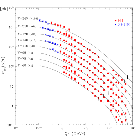
FIG. 8.: $\sigma_{tot}(\gamma^{*}+p)$ in our model. From these data we extracted $Q^{2}_{0T}=0.7\div 0.9\,\,GeV^{2}$ and $Q^{2}_{0L}<0.4\,\,GeV^{2}$. The vertical line corresponds to $x=0.01$.

B $\mathbf{F_{2}}$.

Our main conclusion that the global features of $F_{2}$ is not very sensitive to the contributions of the SC from distances $r_{\perp}\,<\,r^{sep}_{\perp}$ [7]. In Fig.  9 we plot the result of our estimates for low $Q^{2}=1.5\div 6.5\,GeV^{2}$, for higher $Q^{2}$ the shadowing corrections are even smaller.

FIG. 9.: $F_{2}$ with ( dashed line) and without SC in our model. SC has been taken into account for distances shorter than the separation scale ($r_{\perp}<r^{sep}_{\perp}=1/Q_{0}$).

C $\mathbf{xG(Q^{2},x)}$

Our calculations for $xG(x,Q^{2})$ has been discussed in section V1 ( see Figs. 6-a - 6-c and Ref. [7] ). One can see from these figures that unlike the case of $F_{2}$, the shadowing corrections are rather large and they tame the increase of the gluon density. Actually, all indications of high density QCD effects, that we see in the HERA data and will discuss below, are due to strong screening in the gluon channel.

D $\mathbf{F_{2}}$ Slope.

We consider the $Q^{2}$ behavior of the $F_{2}$ slope, $\frac{dF_{2}}{dlnQ^{2}}$, as the best experimental indication of the strong SC or other effects of high density QCD. Our study [20, 25] shows that none of available parameterization of the DGLAP equation can reproduce the experimental data, while our model does this. More than that, two different parameterization such as GRV’94 and GRV’98 both describe the data well after taking into account SC in the framework of our model. Fig. 10 shows the comparison of the GRV’98 parameterization with the H1 data. One can see that GRV’98 which was invented to describe ZEUS data ( Caldwell-plot) failed to fit H1 results but in our model we can fit H1 data without any additional change of parameters.

Fig. 11 presents the ‘ideal’ Caldwell plot from the point of the gluon saturation (see section VII): the $F_{2}$ slope as function of $Q^{2}$ at fixed $x$. One can see two features in this figure: (i) our model describes the HERA data quite well; and (ii) the data as well as our calculation do not show any maximum which could be interpret as a saturation scale. Our model is also able to describe the $Q^{2}$ behaviour of the $F_{2}$ at fixed $W$ which shows maxima. It means that the maxima in the fixed $W$ plot does not reflect the saturation phase of the parton cascade but are an artifact of the particular choice of the kinematic variable.

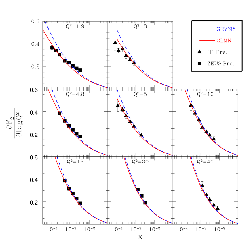
FIG. 10.: $F_{2}$-slope in GRV’98 and in our model with GRV’98 input for gluon structure function. Data are taken from figures of Ref. [35] and from Ref. [36].

FIG. 11.: The $F_{2}$ slope at fixed $x$ versus $Q^{2}$.Data are taken from figures of Ref. [35] and from Ref. [36].

We have also studied an alternative approach, namely, the Donnachie-Landshoff model for matching the “soft” and the “hard” interactions [37]: the sum of “soft” and “hard” Pomerons (see Fig. 12). One can see that this model is as successful in describing the data as is our model. This means that at the moment we cannot claim that the data show a saturation effect. We have a much more modest claim: The current data can be described in two different approaches, either due to gluon saturation or due to matching between “soft” and “hard” contributions ( “soft” and “hard” Pomerons ) but at rather large momenta ( about $1-2\,GeV$ ). In spite of the fact that we failed to arrive at a unique conclusion one can see that measuring the $F_{2}$ slope gives new and interesting information about QCD dynamics.

FIG. 12.: The $F_{2}$ slope at fixed $W$ versus $Q^{2}$. Curves are calculated In Donnachie-Landshoff model [37]. Data are taken from figures of Ref. [35] and from Ref. [36].

E Energy dependence of the inclusive diffraction cross section $\sigma^{diff}_{tot}$ and the ratio $\mathbf{\frac{\sigma_{diff}}{\sigma_{tot}}}$.

In a saturation approach the typical distances that are dominant in the diffractive production, are of the order of the saturation scale $r^{saturation}_{\perp}$ [1, 22, 39], unlike the total cross section where they are of the order of $(1/Q)$.n One can see this directly from Fig. 2 which shows that in the saturation region a hadron appears as a diffraction grid of size $r^{saturation}_{\perp}$. This fact is in a perfect agreement with the HERA experimental data [38] as well as with our estimates [22].

However, we cannot reproduce in our model[23] the experimentally observed fact that the ratio $\sigma^{diff}_{tot}/\sigma_{tot}$ is almost energy independent. The dependence on energy in our calculations stems partly from distances shorter than $0.3fm$ (see Ref. [23] for details ) where we can trust the DGLAP evolution equations. The DGLAP evolution was included in our model in contrast to the Golec-Biernat and Wusthoff model [40] which includes the saturation scale but has a very oversimplified behaviour at short $r_{\perp}$ ($\sigma_{dipole}\propto r^{2}_{\perp}$ ).

$\mathbf{Q^{2}=8\,GeV^{2}}$	$\mathbf{Q^{2}=14\,GeV^{2}}$
$\mathbf{Q^{2}=27\,GeV^{2}}$	$\mathbf{Q^{2}=60\,GeV^{2}}$

FIG. 13.: $\sigma^{diff}/sigma_{tot}$ vesus energy in our model. Solid line is total contribution, dashed line is $q\bar{q}$ and dotted line is $q\bar{q}+G$ contributions.

F Energy dependence of J/$\mathbf{\Psi}$ production.

We claim that the energy behaviour of the exclusive vector meson production, especially, J/$\Psi$-production is very discriminating with respect to SC (see Fig.  14). In spite of large errors related to uncertainties due to our poor knowledge of the wave function of vector mesons, this uncertainty contributes mostly to the normalization of the cross section while the energy slope is still a source of the information on the SC. We believe that at the moment there is no parameterization of the DGLAP evolution equation which is able to describe simalteneously the $F_{2}$-slope and the energy dependence of the J/$\Psi$ photo production where a huge amount of new data has been accumulated ( see Ref. [25] and references therein for more details ).

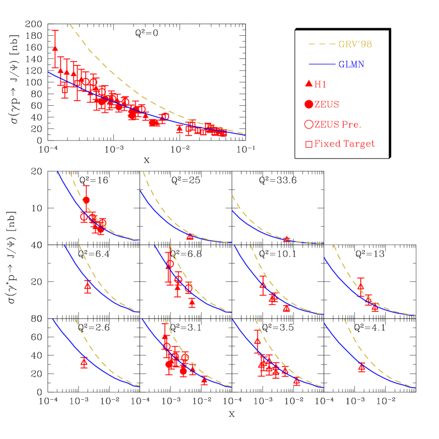
FIG. 14.: Examples of the description of J/$\Psi$ DIS and photo production. We got excellent n.d.f. $<$ 1.

G $\mathbf{t}$ - behaviour of hard diffractive leptoproduction of vector meson.

As has been mentioned, in our model we generate a shrinkage of the diffraction peak (see Fig. 15 ) as well as a damping of the energy dependence. We want to draw the readers attention to the fact that we expect a characteristic $t$-dependence with possible minimum around $|t|=0.8\div 1.2\,\,GeV^{2}$.

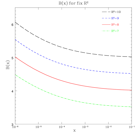
fig.15-a	Fig. 15-b

FIG. 15.: The energy behaviour of the diffraction slope ( FIg. 15-a) and the $t$ - dependence (Fig. 15-b) for J/$\Psi$ photo production. Fig.15-b corresponds to the two radii model for the impact parameter dependence [24] of the profile function which provides a better description of the experimental data. Fig. 15-a is plotted for one radius model. The experimental data are taken from [41].

XI Searching for new observables:

A $\mathbf{\sigma(\gamma\,\,\gamma^{*})}$.

The interaction of two virtual photons provides a unique opportunity to measure both the property of the BFKL Pomeron [42] as well as to explore the saturation region. By now we have checked that our model is able to describe[21] current experimental data for the $\gamma\gamma^{*}$ total cross section[43] with the same parameters that we used for DIS with the nucleon target (see Fig.  16 ). However, we cannot reproduce in our approach the experimental data for the cross section of two virtual photons with $Q^{2}_{1}\,\approx Q^{2}_{2}\,>1\,GeV^{2}$. Perhaps, we need to improve our approach including the BFKL contribution.

B Maxima in ratios.

In our attempt to find an improved observable which will be more sensitive to the saturation scale we study the $Q^{2}$ behaviour of the ratios: $F_{L}/F_{T}$ and $F^{D}_{L}/F^{D}_{T}$ for longitudinal and transverse structure function for inclusive DIS and for diffraction in DIS[44]. We found that these ratios have maxima at $Q^{2}=Q^{2}_{max}(x)$ which are moving as a function of $x$. In Fig. 17 we have plotted some examples of these ratios and the behaviour of $Q_{max}(x)$. It appears that $Q_{max}(x)$ is a simple function of the saturation scale $Q^{2}_{s}(x)$ of Eq. (2).

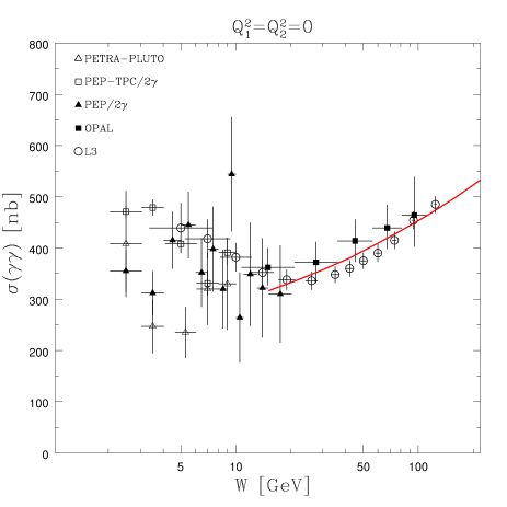
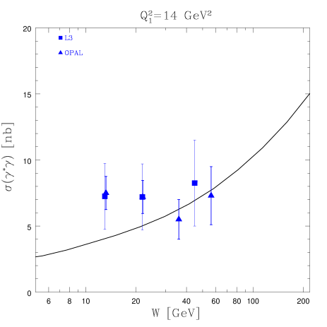
FIG. 16.: The description of $\gamma^{*}\,\gamma^{*}$ total cross section at different values of the photon vituality in our model. The experimental data are taken from Ref. [43].

FIG. 17.: The ratio of $F^{D}_{L}/F^{D}_{T}$ as function of $Q^{2}$ at different values of $x$ and the behavior of $Q^{2}_{max}(x)$ as function of $x$.

C Higher twist contributions.

As we have mentioned, one of the attractive features of our model is the fact that we are able to describe the higher twist contribution in accordance with all known theoretical information. Our calculations confirm the result of Ref.[45] that there is an almost full cancellation of higher twist contribution in $F_{2}$ while they give substantial contributions separately in $F_{L}$ and $F_{T}$ as well as in $F^{D}$. We hope, that the twist analysis will help us to find a scale when the higher twist contribution will be of the order of the leading one. It is well known [1], that in a saturation approach at $Q^{2}=Q^{2}_{s}(x)$ all twist contributions are of the same order. Therefore, our twist analysis will assist in finding a kinematic range of $Q^{2}$ and $x$ where the higher twist should be important and where we expect a manifestation of the gluon saturation.

XII Our plans for the near future.

We list here the problems that we have started to work on:

1. Large $p_{t}$-jet production in photo production. The first calculation indicates a maximum at the saturation scale in $p_{t}$ -spectrum;

2. Heavy quark production and especially open charm production will appear soon;

3. Using our model we intend to calculate the inclusive observables and to examine their sensitivity to SC;

4. We have started, and we are going to continue, to check our approach with the $\gamma^{*}\gamma^{*}$- data on total cross section;

5. The calculations for gluon structure function as well as for $F_{2}$ for nuclear targets has been performed, as well as predictions for the total diffractive cross sections for DIS with nuclei. We have extended our twist analysis to DIS with nucleus[28] to see whether we will be able to separate the higher twist contribution using A-dependence. We have started to calculate all above mentioned observables for DIS with a nuclear target, hoping that the future experiment for DIS with nuclei will open a new dimension in our investigation of the saturation phenomenon and will be complementary to HERA data.

XIII Feedback for theory:

It should be mentioned that our model or a similar type of approach is needed to solve the nonlinear evolution equation that have been discussed in section IV. The essential requirements to solve Eq. (3) are:

• a correct initial distribution, which should be of the eikonal type as was shown by Kovchegov [6];

• values of the parameters that enter Eq. (3), such as the $b_{t}$-distribution and a separation scale;

• a relationship between the dipole scattering amplitude $a^{el}(r^{2}_{\perp},b_{t};x)$ and the gluon structure function.

Our model provides an answer to all formulated questions and can be used as an initial distribution for the nonlinear evolution equation (see Eq. (3) ). Indeed, our model gives the eikonal description of the experimental data which is suited to be used as the initial condition for Eq. (3). The only item that we need to add is the relation between the gluon structure function and the dipole scattering amplitude. This relation is a natural generalization of Eq. (13), namely,

$$xG(x,\frac{4}{r^{2}_{\perp}})\,\,\,\,=\,\,\,\,\frac{4R^{2}}{\pi}\,\int\,\,d^{2}b_{t}\,\int^{1}_{x}\,\frac{dx^{\prime}}{x^{\prime}}\,\int^{\infty}_{r_{\perp}}\,\,\frac{dr^{2}_{\perp}}{r^{4}_{\perp}}\,\,2\,\,Im\,\,a(r^{2}_{\perp},b_{t};x)\,\,.$$ (19)

A similar relation for the $F_{2}$ structure function stems directly from the relationship between the measured cross section ( $\sigma(\gamma^{*}p)$ ) and $F_{2}$ ( $\sigma(\gamma^{*}p)=\frac{4\pi^{2}}{Q^{2}}F_{2}$ ) and from Eq. (10) and Eq. (11). We assumed that for a gluon probe [13] we have the same relation between the gluon structure function and the measured cross section. It should be stressed that Eq. (19) coincides with the definition of the gluon structure function in the DGLAP limit.

Based on the model developed for the initial condition we will attempt to solve the evolution equation ( see Eq. (3)) and so provide reliable estimates for the structure functions in the LHC kinematic region.

XIV Comparison with other models:

the models that are on the market fall into two classes: (i) models that introduce the saturation scale in addition to the separation one ( see our model and Refs. [40, 46, 47] ), and (ii) models that only have a separation scale (see Refs.[14, 37, 46, 48]). We discuss here only models that reproduce the same data or almost the same data as ours with a chi squared of approximately the same value. There are two such models

Our model and Golec-Biernat and Wusthoff model [40] are in the first class: both of them introduce a saturation scale and we will discuss the difference between them a little later. The Forshaw, Kelley and Shaw model[48] suggested a different approach based on ideas of Donnachie and Landshoff model [14, 37]. They use Eq. (10), and for the dipole cross section they suggest the sum of “soft” and “hard” contribution:

$$\sigma_{dipole}(r^{2}_{\perp},W)\,\,=\,\,f_{S}(r_{\perp})\,W^{\lambda_{S}}\,\,+\,\,f_{H}(r_{\perp}\,\,(r^{2}_{\perp}\,\,W^{2})^{\lambda_{H}}\\ ,$$ (20)

with the following limits of

$$f_{S}(r_{\perp})\,\,\,\, \longrightarrow \,\,\,\,Const\,\,\,at\,\,\,\,r_{\perp}\,\geq\,0.8\div\,1\,fm\,\,;$$ (21)

$$f_{H}(r_{\perp})\,\,\,\, \longrightarrow \,\,\,\,r^{2}_{\perp}\,\,\,at\,\,\,\,r_{\perp}\,\leq\,028\div\,0.3\,fm\,\,.$$ (22)

Therefore, in Eq. (20) one can recognize the “soft” Pomeron in the first term, while the second one at short distances ( $r_{\perp}\ll r^{sep}_{\perp}$ ) depends on $x$ as it should for the “hard” contribution.

The success of this model shows us that the HERA data alone cannot distinguish between a rather small separation scale and saturation of the gluon density. In this model “hard” and “soft” are compatible at $r_{\perp}\approx 0.4\,fm$ which is rather small.

There is no difference in principle between the Golec-Wusthoff model and ours since both of them use the same physical picture that follows from the high density QCD. However, in our model the saturation scale can be calculated (see Eq. (2) ) and all our results have the correct DGLAP limit at short distances. On the other hand, Golec-Wusthoff model introduces the saturation scale as a phenomenological parameter, has an extremely simple form and reproduces the HERA data on the energy behaviour of ratio for $\sigma^{diff}_{tot}/\sigma_{tot}$. In other words, Golec-Wusthoff model investigates the extreme limit: all physics observed at HERA is related to a saturation scale. It is very encouraging that such a rudimentary idea does not contradict all experimental data from HERA.

In Fig. 18 we plot the ratio of our dipole cross section to Golec-Wusthoff one. More work is needed to understand how much of the disagreement stems from attractive features of our models such as correct matching with the DGLAP evolution equation, and how much of them can be explained by the fact that our model underestimates the value of SC at rather low $Q^{2}\approx 1\div 2\,GeV^{2}$.

Fig. 18-a	Fig.18-b

FIG. 18.: The ratio of our dipole cross section to Golec-Biernat and Wusthoff dipole cross section at $x=10^{-3}$ versus $r^{2}_{\perp}(GeV^{-2})$ for total cross section ( Fig.18-a) and for diffractive cross section (Fig.18-b).

It is incorrect to say that it is not possibile to distinguish one model from another. For example, for diffractive production it is important to take into account the diffractive dissociation in $q\bar{q}G$ channel. This channel can be considered as the production of a dipole but with a charge which is twice larger ( for $N_{c}>1$ ) than for a $q\bar{q}$ dipole. In spite of this fact in the two models [40, 48] the dipole for $q\bar{q}G$ - channel was treated in the same way as $q\bar{q}$ dipole ( in MFGS model[47] it has not yet been considered ). In our model which is based on the correct matching with the pQCD result, the propagation of $q\bar{q}G$ - dipole is quite different than for a quark-anti quark pair. This means that these models should have different predictions for jet production in the diffractive dissociation processes.

XV Our answer:

In our opinion HERA has reached a high density QCD domain because: (i) HERA data display a large value of the gluon structure function; (ii) no contradictions with the asymptotic predictions of high density QCD have been observed; and (iii) the numerical estimates of our model give a natural description of the size of the deviation from the usual DGLAP explanation. However, we know the main shortcoming of our statement, which is that most of the observed indications of high density effects can be described alternatively without assuming a saturation scale, but by matching “soft” and “hard” processes at rather short distances. We want to stress three aspects:

1. The alternative approaches cannot describe or, perhaps, have not described all data and, in particular, the energy dependence of the J/$\Psi$ photon and DIS production [25]. We found that a simultaneous analysis of this reaction and of the $F_{2}$ slope cannot be done without employing shadowing corrections;

2. The gluon saturation is not an additional postulate of pQCD, but follows from the QCD evolution equations in the high parton density kinematic region, and our model describes the solution to these equations;

3. The gluon saturation leads to the simplest Golec-Biernat and Wusthoff model which gives an impressive description of the data.

The fact that one can describe the HERA data without assuming gluon saturation is not very surprising as the saturation scale in the HERA kinematic region is $Q^{2}_{s}(x)=1\div 3GeV^{2}$ while the typical scale for the “soft” Pomeron is also not very small and can be as large as $4\,GeV^{2}$ [49].

We hope that the simultaneous analysis of all HERA data , which we plan to undertake, will be consistent only with the saturation approach. In doing so we have to rely on the hdQCD evolution equations rather then on models.

XVI Predictions for THERA:

As we have pointed out it is rather dangerous to discuss predictions for lower $x$ in our model, since the model should be replaced by the solution of the correct evolution equation of Eq. (3). However, in this section we summarize some of our predictions for as low $x$ as $x\rightarrow 10^{-6}$ since this region of $x$ is under detailed discussion due to plans of the THERA extension of TESLA project [50]. We would like to recall that our predictions underestimate the solution to the nonlinear evolution equation, but we can use them as a first estimate in our search for collective phenomena in high parton density system.

The unitarity boundary and THERA kinematic region:

We start from the prediction which, in principle, does not depend on the exact form of the correct evolution equation, namely, from the unitarity boundary for the $F_{2}$ and $xG(x,Q^{2})$ structure functions. This problem has been considered in Ref. [51] and it turns out that we have the following unitarity boundaries for $F_{2}$ and $xG(x,Q^{2})$:

$$\frac{\partial F_{2}(x,Q^{2})}{\partial\ln Q^{2}}\,\,\, < \,\,\,\frac{1}{3\,\pi^{2}}\,\,Q^{2}\,R^{2}\,\,;$$ (23)

$$\frac{\partial^{2}xG(x,Q^{2})}{\partial\ln Q^{2}\,\,\partial\ln(1/x)}\,\,\, < \,\,\,\frac{2}{\pi^{2}}\,\,Q^{2}\,R^{2}\,\,;$$ (24)

where $R$ is the nucleon radius. Actually, in Eq. (23) and Eq. (24) we need to $R^{2}=<b^{2}_{t}>_{F_{2}}$ and $R^{2}=<b^{2}_{t}>_{xG}$, respectively (see Fig. 7). As it shown in Fig.7, the interaction radii depend on energy and $Q^{2}$ but the dependence is so weak that we can neglect it in the first approximation.

In Fig. 19 we plot Eq. (24) and the predictions for $F_{2}$-slopes in GRV[32],in MRS [31] and in CTEQ [30] parameterizations. One can see that the $F_{2}$-slope in the DGLAP evolution equations reaches the unitarity boundary at $Q^{2}\leq 3\,GeV^{2}$ for $x=10^{-5}$ and even for $Q^{2}\leq 10\,GeV^{2}$ for $x=10^{-6}$.

Fig. 20 shows the comparison of the DGLAP evolution equations with the unitarity boundary for the case of gluon structure function. In Fig. 20 Eq. (24) is modified using the DGLAP evolution equation in the region of low $x$, namely,

$$\frac{\partial^{2}xG^{DGLAP}(x,Q^{2})}{\partial\ln Q^{2}\,\,\partial\ln(1/x)}\,\,\,=\,\,\frac{N_{c}\alpha_{S}(Q^{2})}{\pi}\,\,\,xG^{DGLAP}(x,Q^{2})\,\,.$$ (25)

Using Eq. (25) one can rewrite Eq. (24) in the form

$$xG^{DGLAP}(x,Q^{2})\,\,\,<\,\,\,\frac{2}{\pi\,N_{c}\,\alpha_{S}(Q^{2})}\,\,Q^{2}\,R^{2}\,\,.$$ (26)

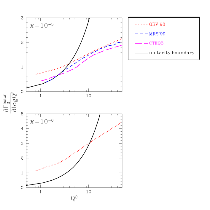
FIG. 19.: The unitarity boundary for $F_{2}$-slope and predictions in GRV,MRS and CTEQ parameterizations for the solution of the DGLAP evolution equations in THERA kinematic region.

Based on Fig. 20 we are not optimistic of finding gluon saturation for the unitarity constrains on the gluon structure function in THERA kinematic region. The $F_{2}$-slope at lower $x$ ($x\approx 10^{-6}$) will give more reliable limit on the gluon saturation.

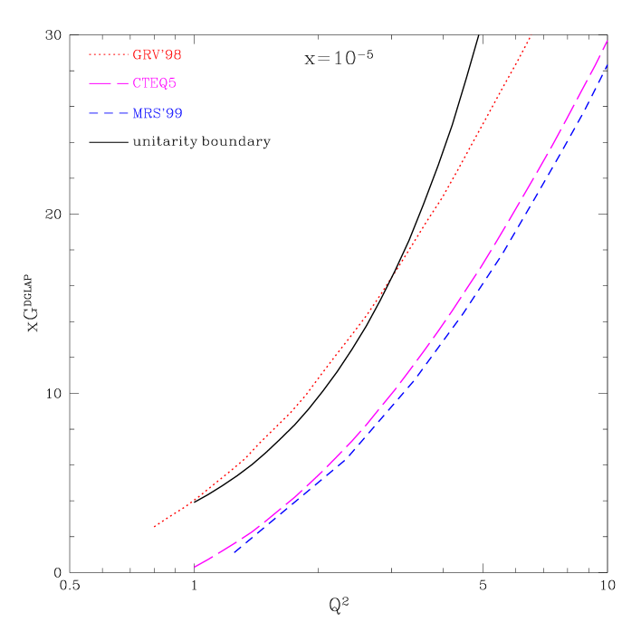
FIG. 20.: The unitarity boundary for $xG(x,Q^{2})$ and predictions in GRV,MRS and CTEQ parameterizations of the solution of the DGLAP evolutions equations in THERA kinematic region.

However, the calculations, given in Fig. 6 using both our model and the solution to the Eq. (3), suggest that the corrections to at least $xG$ is rather large in the THERA kinematic region.

$$\mathbf{\frac{\partial F_{2}}{\partial\ln Q^{2}}}$$

The THERA kinematic region provides a new opportunity to check the value of SC using the $F_{2}$ slope. At least, the THERA data would help us to differentiate between two approaches: our approach, based on the gluon saturation at low $x$ and the approach based on the matching between “soft” and “hard” interaction with a sufficiently large momentum scale for “soft” contribution. Fig.  21 shows the predictions for the $F_{2}$-slope in our approach ( GLMN in figure ) and the Donnachie-Landshoff approach[37]. The difference is rather large and can be measured.

FIG. 21.: The prediction for the $F_{2}$-slope in our approach (GLMN) and in Donnachie-Landshoff approach (DL).

J/$\mathbf{\Psi}$ production:

Fig.  22 shows that the difference between our predictions and the DGLAP increase at the THERA kinematic region, which leads us to speculate that we will see gluon saturation at THERA.

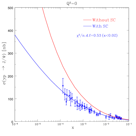
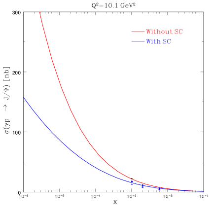
FIG. 22.: Predictions for J/$\Psi$ production in THERA kinematic region together with available experimental data.

Maxima in the ratios and the higher twist contributions

Fig. 17 shows that we expect a characteristic behaviour of the ratio $F^{D}_{L}/F^{D}_{T}$ as a function of $Q^{2}$. It turns out to be wider than at higher $x$ and the maximum occurs at the value of $Q^{2}_{max}\approx 6\div 7\,GeV^{2}$. Such a large value of $Q^{2}_{max}$ makes the calculations reliable and we expect that the measurement of this observable in the THERA kinematic region will help us to extract the value of the saturation scale from the experimental data. In THERA kinematic region ( at $x\approx 10^{-5}$ ) we expect that the higher twist contributions to be of the same order as the leading twist ones at sufficiently high value of $Q^{2}$, namely, for $F_{L}$ and for $F^{D}_{T}$ this value of $Q^{2}$ is about $5\div 7\,GeV^{2}$ while for $F^{D}_{L}$ it is even larger, about $15\,GeV^{2}$. The fact that the higher twist contributions become visible at large value of $Q^{2}$ lead to a visible violation of the usual DGLAP evolution approach which should be possible to measure.

REFERENCES

-
[1]
L.V. Gribov, E.M. Levin and M.G. Ryskin, Phys. Rep
100 (1983) 1;
A.H. Mueller and J. Qiu, Nucl. Phys. B268 (1986) 427;
L. McLerran and R. Venugopalan,Phys. Rev. D49 (1994) 2233,3352, 50 (1994) 2225, 53 (1996) 458, 59 (1999) 094002. - [2] V.N. Gribov, Sov. Phys. JETP 30 (1970) 709.
-
[3]
E. Levin and M.G. Ryskin, Phys. Rep. 189 (19267) 1990;
J.C.Collins and J. Kwiecinski, Nucl. Phys. B335 (1990) 89;
J. Bartels, J. Blumlein and G. Shuler, Z. Phys. C50 (1991) 91;
E. Laenen and E. Levin, Ann. Rev. Nucl. Part. Sci. 44 (1994) 199 and references therein;
A.L. Ayala, M.B. Gay Ducati and E.M. Levin, Nucl. Phys. B493 (1997) 305, B510 (1990) 355;
Ia. Balitsky, Nucl.Phys. B463 (1996) 99;
Yu. Kovchegov, Phys. Rev. D54 (191996) 5463, D55(1997) 5445, D60(2000) 034008, D61 (2000)074018;
A.H. Mueller, Nucl. Phys. B572(2000)227, B558 (1999) 285;
Yu. V. Kovchegov, A.H. Mueller, Nucl. Phys. B529 (1998) 451;
E. Levin and K. Tuchin, Nucl. Phys. B573(2000) 833. - [4] A.H. Mueller, Nucl. Phys. B415 (1994) 373.
-
[5]
J. Jalilian-Marian, A. Kovner, L. McLerran and H.
Weigert, Phys. Rev. DD55 (1997) 5414;
J. Jalilian-Marian, A. Kovner and H. Weigert, Phys. Rev. D59 (1999) 014015;
J. Jalilian-Marian, A. Kovner and H. Weigert, Phys. Rev. D59 (1999) 014015;
J. Jalilian-Marian, A. Kovner, A. Leonidov and H. Weigert, Phys. Rev. D59 (1999) 014014,034007, Erratum-ibid. Phys. Rev. D59 (1999) 099903;
A. Kovner, J.Guilherme Milhano and H. Weigert, OUTP-00-10P,NORDITA-2000-14-HE, hep-ph/0004014;
H. Weigert, NORDITA-2000-34-HE, hep-ph/0004044. - [6] Ia. Balitsky, Nucl.Phys. B463 (1996) 99; Yu. Kovchegov, Phys. Rev. D60 (191000) 034008.
- [7] A.L. Ayala, M.B. Gay Ducati and E.M. Levin, Nucl. Phys. B493 (1997) 305, B510 (1998) 355.
- [8] L.McLerran, “ Renormalization Group Equations, Saturation, and the Colored Glass Condensate”, talk given at WS “QCD in a nuclear environment”, August 3-5, Regensburg, Germany.
-
[9]
Yu. V. Kovchegov, Phys.Rev. D61 (2000) 074018;
E. Levin and K. Tuchin, Nucl.Phys. B573 (2000) 833;
M. Braun, Eur.Phys.J. C16 (2000) 337. - [10] E. Levin and L. Frankfurt, JETP Lett. 2 (1965) 65; H. J. Lipkin and F. Scheck, Phys. Rev. Lett. 16 (1966) 71.
- [11] A. Zamolodchikov, B. Kopeliovich and L. Lapidus, JETP Lett. 33 (1981) 595;
- [12] E.M. Levin and M.G. Ryskin, Sov. J. Nucl. Phys. 45 (1987) 150.
- [13] A. H. Mueller, Nucl. Phys. B335 (1990) 115.
- [14] A. Donnachie, P. V. Landshoff,Phys. Lett. B296 (1992) 227; B437(1998) 408 and references therein.
- [15] G. Cvetic, D. Schildknecht and A. Shoshi,Acta Phys.Polon. B30 (1999) 3265, hep-ph/9910379 and references therein.
- [16] E. Shuryak and T. Schafer, Ann.Rev.Nucl.Part.Sci. 47 (1997) 359 and references therein.
-
[17]
E. Gotsman, E. Levin, U. Maor and E. Naftali, Eur.Phys.J. C10 (1999) 689;
E. Gotsman, E. Levin and U. Maor, Eur.Phys.J. C5 (1998) 303. -
[18]
N.N. Nikolaev and B.G. Zakharov, Z. Phys. C49 (1991) 607;
E.M. Levin, A.D. Martin, M.G. Ryskin and T. Teubner, Z. Phys. C74 (1997) 671. - [19] E. Gotsman, E. Levin and U. Maor, Phys.Lett. B379 (1990) 186.
-
[20]
E. Gotsman, E. Levin, U. Maor and E. Naftali,
Nucl.Phys. B539 (1999) 535;
E. Gotsman, E. Levin and U. Maor, Phys.Lett. B425 (1998) 369. - [21] E. Gotsman, E. Levin, U. Maor and E. Naftali, Eur.Phys.J. C14 (2000) 511.
- [22] E. Gotsman, E. Levin and U. Maor, Nucl.Phys. B493 (1997) 354.
- [23] E. Gotsman, E. Levin, M. Lublinsky, U. Maor and K. Tuchin, “ Energy dependence of in DIS and shadowing corrections”, TAUP-2639-2000, Jul 2000, hep-ph/0007261.
- [24] E. Gotsman, E. Levin and U. Maor, Phys.Lett. B403 (1997) 120; Nucl.Phys. B464 (1996) 251.
- [25] E. Gotsman, E. Ferreira, E. Levin, U. Maor and E. Naftali, “ Screening corrections in DIS at low and ” , Talk given at 30th International Conference on High-Energy Physics (ICHEP 2000), Osaka, Japan, 27 Jul - 2 Aug 2000, hep-ph/0007274.
- [26] V.A. Abramovsky, V.N. Gribov and O,V. Kancheli, Sov. J. Nucl. Phys. 18 (1974) 308.
-
[27]
J. Bartels, Phys. Lett. B298 (1993) 204, Z. Phys. C60 (1993) 471;
E.M. Levin, M.G. Ryskin and A.G. Shuvaev, Nucl. Phys. B387 (1992) 589. -
[28]
E. Gotsman, E. Levin, U. Maor, L. McLerran and K. Tuchin, “Higher
twists and maxima for DIS on nuclei in high density QCD”,TAUP-2638-200,
BNL-NT-00-19, Jul 2000, hep-ph/0007258 .
E. Gotsman, E. Levin, M. Lublinsky, U. Maor and K. Tuchin, “Shadowing corrections and diffractive production in DIS on nuclei”, TAUP-2605-99, Nov 1999, hep-ph/9911270. - [29] Yu. V. Kovchegov and L. McLerran, Phys.Rev. D60 (1999) 054025.
- [30] H. L. Lai et al., Eur. Phys. J. C12 (2000) 37;
- [31] A. D. Martin, R. G. Roberts, W. J. Stirling and R. S. Thorne, Eur. Phys. J. C4 (1998) 463.
- [32] M. Gluck, E. Reya and A. Vogt, Eur. Phys. J. C5 (1998) 461.
-
[33]
H1 collaboration: S. Aid et al., Nucl. Phys. B470 (1996) 3; C, Adolf et al.,
Nucl. Phys. B497 (1997) 3;
ZEUS collaboration: M. Derrick et al., Z. Phys. C72 (1996) 399; J. Breitweg et al., Phys. Lett. B407 (1997) 432; DESY-00-071, hep-ex/0005018. -
[34]
A. M. Cooper-Sarkar, R. C. E. Devenish and A. De Roeck, Int. J. Mod.
Phys. A13 (1998) 33;
H. Abramowicz and A. Caldwell, Rev. Mod. Phys. 71 (1999) 1275. - [35] M. Klein (H1 collaboration), “Structure Functions in Deep Inelastic Lepton-Nucleon Scattering” Talk at Lepton-Photon Symposium, Stanford, August 1999, hep-ex/0001059.
-
[36]
B. Foster (ZEUS Collaboration), Invited talk, Royal Society Meeting,
London, May 2000;
ZEUS collaboration: J. Breitweg et al., Phys. Lett. B487 (2000) 53. - [37] A. Donnachie and P.V. Landshoff: Phys. Lett. B437 (1998) 408; Phys. Lett. B470 (1999) 243.
-
[38]
H1 Collaboration: C. Adloff et al., Z. Phys. C76 (1997) 613;
ZEUS Collaboration: J. Breitweq et al., Eur. Phys. J. C6 (1999) 43. -
[39]
E. Levin and M. Wusthoff, Phys.Rev. D50
(1994) 4306;
M. Wusthoff and A.D. Martin, J.Phys. G2 (1999) R309. - [40] K. Golec-Biernat and M. Wusthoff, Phys. Rev. D59 (1999) 014017; D60 (1999) 114023; K.Golec-Biernat,Talk at 8th International Workshop on Deep Inelastic Scattering and QCD (DIS 2000), Liverpool, England, 25-30 Apr 2000,hep-ph/0006080.
-
[41]
ZEUS collaboration: J. Breitweg et al., Eur. Phys. J. C14
(2000) 213.
H1 Collaboration: C. Adloff et al.,Phys. Lett. B483 (2000) 36. -
[42]
J. Bartels, A. De Roeck and H. Lotter, Phys. Lett. B389 (1996) 742;
J. Bartels, A. De Roeck, C. Ewerz and H. Lotter, ”The gamma* gamma* total cross section and the BFKL pomeron at the 500-GeV e+ e- linear collider”, hep-ph/9710500;
S. J. Brodsky, F. Hautmann and D. E. Soper, Phys. Rev. Lett. 78 (1997) 803. -
[43]
PLUTO collaboration: C. Berger et al.,
Phys. Lett. B149 (191984) 42, Z. Phys. C26 (1984) 353;
PC/Two Gamma Collaboration: H. Aihara et al., Phys. Rev. D41 (1990) 2667;. D. Bintingeret al., Phys. Rev. Lett. 54 (1985) 763;
OPAL Collaboration: G. Abbiendi et al., Eur. Phys. J. C14 (2000) 1;
L3 Collaboration: M. Acciarri et al., Phys. Lett. B408 (1997) 450; - [44] E. Gotsman, E. Levin, L. McLerran and K. Tuchin, “Higher twists and maxima for DIS on proton in high density QCD”, TAUP-2644-2000, BNL-NT-00-20, Aug 2000, hep-ph/0008280.
-
[45]
B. Badelek and J. Kwiecinski, Phys.Lett. B418
(1998) 229 and references therein;
J. Bartels, K. Golec-Biernat and K. Peters, “ An estimate of higher twist at small and low based upon a saturation model”, DESY-00-038, Mar 2000, hep-ph/0003042. - [46] M.F. McDermott,“ The dipole picture of small physics ( a summary of the Amirim meeting)”, hep-ph/0008260.
- [47] M. McDermott, L. Frankfurt, V. Guzey and M. Strikman,”Unitarity and the QCD-improved dipole picture”, hep-ph/9912547.
- [48] J. R. Forshaw, G. Kerley and G. Shaw, Phys.Re. D60 (1999) 074012,Nucl. Phys. A675 (2000) 80.
-
[49]
D. Kharzeev and E. Levin, Nucl.Phys. B578 (2000) 351;
Yu. Kovchegov, D. Kharzeev and E. Levin, “ QCD instantons and the soft Pomeron”,BNL-NT-00-18, TAUP-2637-2000, Jul 2000, hep-ph/0007182 ;
B.Z. Kopeliovich, I.K. Potashnikova, B. Povh and E. Predazzi, Phys.Rev.Lett. 85 (2000) 507. - [50] Max Klein, “THERA-electron proton scattering at ”, talk, given at DIS’2000, Liverpool, April 25-30,200; and web-page: www.ifh.de/thera/.
- [51] A.L. Ayala Filho, M.B. Gay Ducati and E.M. Levin,Phys.Lett. B388 (1996) 188.