Current fragmentation in
semiinclusive leptoproduction

Abstract

Current fragmentation in semiinclusive deep inelastic leptoproduction offers, besides refinement of inclusive measurements such as flavor separation and access to the chiral-odd quark distribution functions $h_{1}^{q}(x)=\delta q(x)$, the possibility to investigate intrinsic transverse momentum of hadrons via azimuthal asymmetries.

Leading quark distribution functions

In deep-inelastic leptoproduction (DIS), the soft hadron structure enters via the quark distribution functions. These distribution functions for a quark can be obtained from the lightcone correlation functions Soper77 ; Jaffe83 ; Manohar90 ; JJ92 .

$$\Phi_{ij}(x)=\left.\int\frac{d\xi^{-}}{2\pi}\ e^{ip\cdot\xi}\,\langle P,S|\overline{\psi}_{j}(0)\psi_{i}(\xi)|P,S\rangle\right|_{\xi^{+}=\xi_{\scriptscriptstyle T}=0},$$ (1)

depending on the lightcone fraction of a quark (with momentum $p$), $x=p^{+}/P^{+}$. In particular the At leading order, the relevant part of the correlator is $\Phi\gamma^{+}$

$$(\Phi\gamma^{+})_{ij} = \left.\int\frac{d\xi^{-}}{2\pi\sqrt{2}}\ e^{ip\cdot\xi}\,\langle P,s^{\prime}|\psi^{\dagger}_{+j}(0)\psi_{+i}(\xi)|P,s\rangle\right|_{\xi^{+}=\xi_{\scriptscriptstyle T}=0}$$ (2)

where $\psi_{+}\equiv P_{+}\psi=\frac{1}{2}\gamma^{-}\gamma^{+}\psi$ is the good component of the quark field KS70 .

Explicitly, the matrix $M=(\Phi\gamma^{+})^{T}$ in Dirac space using a chiral representation becomes for a spin 0 target the following 4 $\times$ 4 matrix,

$$M_{ij}=\left\lgroup\begin{array}[]{cccc}f_{1}(x)&0&0&0\\ 0&0&0&0\\ 0&0&0&0\\ 0&0&0&f_{1}(x)\end{array}\right\rgroup$$ (3)

In hard processes only two Dirac components are relevant, one of them righthanded and one lefthanded ($\psi_{R/L}=\frac{1}{2}(1\pm\gamma_{5})\psi$). Restricting ourselves to those states, the matrix for a spin 0 target becomes

$$M_{ij} = \left\lgroup\begin{array}[]{cc}f_{1}(x)&0\\ &\\ 0&f_{1}(x)\end{array}\right\rgroup\begin{array}[]{c}\includegraphics[width=12.80365pt]{mulders-plenaryfig/helur.eps}\\[8.5359pt] \includegraphics[width=12.80365pt]{mulders-plenaryfig/helul.eps}\end{array}$$

For a spin 1/2 target more quark distributions appear in the lightcone correlation function at leading order. In order to include all possible target polarizations, one can employ a spin vector, in which case one obtains

$$M_{ij} = \left\lgroup\begin{array}[]{cc}f_{1}(x)+S_{\scriptscriptstyle L}\,g_{1}(x)&0S_{\scriptscriptstyle T}^{1}+i\,S_{\scriptscriptstyle T}^{2})\,h_{1}(x)\\ &\\ (S_{\scriptscriptstyle T}^{1}-i\,S_{\scriptscriptstyle T}^{2})\,h_{1}(x)&f_{1}(x)+S_{\scriptscriptstyle L}\,g_{1}(x)\end{array}\right\rgroup\begin{array}[]{c}\includegraphics[width=12.80365pt]{mulders-plenaryfig/helur.eps}\\[8.5359pt] \includegraphics[width=12.80365pt]{mulders-plenaryfig/helul.eps}\end{array}$$

Equivalently, and for our purposes more instructive, one can also express $M$ as a $4\times 4$ matrix in quark $\otimes$ nucleon spin space,

$$M^{\rm(prod)}\ = \left\lgroup\begin{array}[]{cccc}f_{1}+g_{1}&0&0&2\,h_{1}\\ &&&\\ 0&f_{1}-g_{1}&0&0\\ &&&\\ 0&0&f_{1}-g_{1}&0\\ &&&\\ 2\,h_{1}&0&0&f_{1}+g_{1}\end{array}\right\rgroup\ \begin{array}[]{c}\includegraphics[width=22.76228pt]{mulders-plenaryfig/helrr.eps}\\[8.5359pt] \includegraphics[width=22.76228pt]{mulders-plenaryfig/hellr.eps}\\[8.5359pt] \includegraphics[width=22.76228pt]{mulders-plenaryfig/helrl.eps}\\[8.5359pt] \includegraphics[width=22.76228pt]{mulders-plenaryfig/helll.eps}\end{array}$$

Note that the distribution functions exist for each quark flavor. The functions are also denoted $f_{1}^{q}(x)=q(x)$, $g_{1}^{q}(x)=\Delta q(x)$ and $h_{1}^{q}(x)=\delta q(x)$. The three functions are independent. From the fact that any forward matrix element of the above matrix represents a density, one derives positivity bounds Soffer95 ,

$$f_{1}(x)\geq 0$$ (28)

$$|g_{1}(x)|\leq f_{1}(x)$$ (29)

$$|h_{1}(x)|\leq\frac{1}{2}\left(f_{1}(x)+g_{1}(x)\right)\leq f_{1}(x).$$ (30)

As can be seen $h_{1}(x)$ involves a matrix elements between left- and right-handed quarks, it is chirally odd JJ92 . This implies that it is not accessible in inclusive DIS, where the hard scattering part does not change chirality except via (irrelevant) quark mass terms.

By choosing a different basis of quark states, $\psi_{\uparrow/\downarrow}=\frac{1}{2}\left(1+\gamma_{5}\gamma^{1}\right)\psi$ and nucleon transverse spin states (along the x-axis),

$$|N,\uparrow/\downarrow\rangle=\frac{1}{\sqrt{2}}\left(|N,+\rangle\pm|N,-\rangle\right),$$ (31)

one obtains the (equivalent) matrix

$$M^{\rm(prod)}\ = \left\lgroup\begin{array}[]{cccc}f_{1}+h_{1}&0&0&g_{1}+h_{1}\\ &&&\\ 0&f_{1}-h_{1}&g_{1}-h_{1}&0\\ &&&\\ 0&g_{1}-h_{1}&f_{1}-h_{1}&0\\ &&&\\ g_{1}+h_{1}&0&0&f_{1}+h_{1}\end{array}\right\rgroup\ \begin{array}[]{c}\includegraphics[width=12.80365pt]{mulders-plenaryfig/helpp.eps}\\[2.84544pt] \includegraphics[width=12.80365pt]{mulders-plenaryfig/helmp.eps}\\ \includegraphics[width=12.80365pt]{mulders-plenaryfig/helpm.eps}\\[2.84544pt] \includegraphics[width=12.80365pt]{mulders-plenaryfig/helmm.eps}\end{array}$$

from which one sees that $h_{1}(x)$ is a transverse spin density.

Leading gluon distribution functions correspond to lightcone correlators with transverse gluon fields,

$$\Gamma^{+\alpha;+\beta}(x)=\left.\int\frac{d\xi^{-}}{2\pi}\ e^{ip\cdot\xi}\,\langle P,S|F^{+\alpha}(0)F^{+\beta}(\xi)|P,S\rangle\right|_{\xi^{+}=\xi_{\scriptscriptstyle T}=0}.$$ (44)

This can be considered as a gluon production matrix, that for a spin 1/2 hadrons is given by

$$M^{\rm(prod)}\ = \left\lgroup\begin{array}[]{cccc}G+\Delta G&0&0&0\\ &&&\\ 0&G-\Delta G&0&0\\ &&&\\ 0&0&G-\Delta G&0\\ &&&\\ 0&0&0&G+\Delta G\end{array}\right\rgroup\ \begin{array}[]{c}\includegraphics[width=22.76228pt]{mulders-plenaryfig/helgpp.eps}\\[8.5359pt] \includegraphics[width=22.76228pt]{mulders-plenaryfig/helgmp.eps}\\[8.5359pt] \includegraphics[width=22.76228pt]{mulders-plenaryfig/helgpm.eps}\\[8.5359pt] \includegraphics[width=22.76228pt]{mulders-plenaryfig/helgmm.eps}\end{array}$$

Here we have used circularly polarized gluon states.

Inclusive DIS experiments have yielded a good knowledge of the unpolarized quark distributions $q(x)$ in a nucleon and via the evolution equations of $G(x)$. Polarized experiments have provided us with measurements of $\Delta q(x)$ and first indications of $\Delta G(x)$.

Semiinclusive leptoproduction

Semiinclusive DIS (SIDIS), in particular one-particle inclusive DIS, can be and also has been used for additional flavor identification. Instead of weighing quark flavors with the quark charge squared $e_{q}^{2}$ one obtains a weighting with $e_{q}^{2}\,D_{1}^{q\rightarrow h}(z_{h})$, where $D_{1}^{q\rightarrow h}$ is the usual fragmentation function for a quark of flavor $q$ into hadron $h$, experimentally accessible at $z_{h}$ = $P\cdot P_{h}/P\cdot q$. possibilities to study intrinsic transverse momentum of partons, quarks and gluons, via azimuthal asymmetries and the appearance of single spin asymmetries via T-odd fragmentation functions.

         

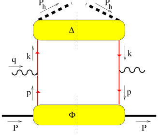
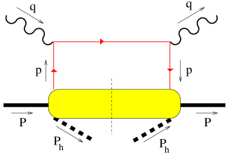
Figure 1: The leading contributions to current (left) and target (right) fragmentation.

Before turning to these topics, I want to address the issue of separation of current fragmentation from target fragmentation, for which the leading order description is illustrated in Fig. 1. While for current fragmentation we can use a description factorizing into distribution and fragmentation functions, target fragmentation involves a more complex soft part, namely fracture functions fracture . Here we want to mention at least one check on the precision of current fragmentation. Up to mass corrections of order $M^{2}/Q^{2}$ one has for current fragmentation the identities

$$x=-\frac{q^{+}}{P^{+}}\approx\frac{Q^{2}}{2P\cdot q}\approx-\frac{P_{h}\cdot q}{P_{h}\cdot P},$$ (57)

$$z=\frac{P_{h}^{-}}{q^{-}}\approx-\frac{2P_{h}\cdot q}{Q^{2}}\approx\frac{P\cdot P_{h}}{P\cdot q}.$$ (58)

Actually incorporation of kinematical $1/Q^{2}$ corrections can be done by calculating the lightcone ratios (first entries in both equations) in a frame in which neither of the hadrons has a transverse momentum component.

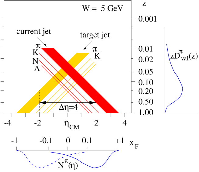
Figure 2: Relation between $z-values$ in fragmentation and CM rapidity for $W$ = 5 GeV.

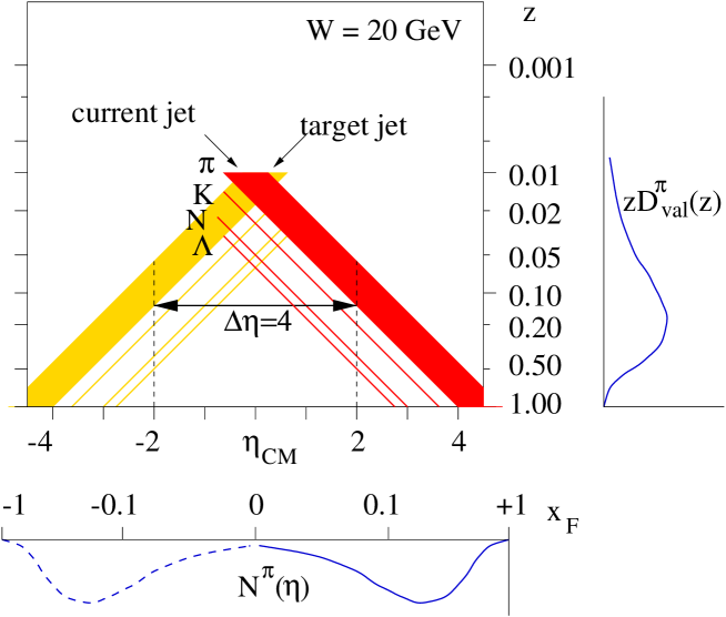
Figure 3: Relation between $z-values$ in fragmentation and CM rapidity for $W$ = 20 GeV.

Based on results in the EMC compilation in ref. Sloan we take a rapidity interval $\Delta\eta\approx 2$ (sometimes referred to as Berger’s criterium) to estimate the z-values for which one is most probably dealing with current fragmentation. For this we construct a plot using the definition of rapidity

$$\eta=\frac{1}{2}\,\ln\left(\frac{P_{h}^{-}}{P_{h}^{+}}\right)=\ln\left(\frac{P_{h}^{-}\sqrt{2}}{M_{h\perp}}\right)=-\ln\left(\frac{P_{h}^{+}}{M_{h\perp}}\right),$$ (59)

where $M_{h\perp}^{2}=M_{h}^{2}+P_{h\perp}^{2}$. For current fragmentation one has $z_{c}=P_{h}^{-}/q^{-}$ while for target fragmentation one is dealing with a ratio $z_{t}=P_{h}^{+}/(1-x)P^{+}$. The proportionality is all we need to deduce that for the center of mass rapidity one has

$$\eta_{cm}=\ln z_{c}+\ln\left(\frac{W}{M_{h\perp}}\right),$$ (60)

$$\eta_{cm}=\ln z_{t}+\ln\left(\frac{W}{M_{h\perp}}\right),$$ (61)

where $W$ is the $\gamma^{\ast}N$ invariant mass, $W=(1-x)y\,s$, fixing the maximum rapidity. For two values of $W$ = 5 and 20 GeV, we have indicated the relation between $z$ and $\eta$ for both current and target fragmentation for a number of hadrons in Figs 2 and 3. For light hadrons the band reflects the influence of the transverse momentum. Looking at the $\Delta\eta$ = 4 difference one can estimate $z$-values above which current fragmentation dominates. Also indicated is how a typical (valence-like) fragmentation function produces a number density in rapidity. Clearly seen is how increased $W$ vastly lowers the $z$-values where one may expect to deal with current fragments.

Leading quark distribition and fragmentation functions in SIDIS

While the distribution functions in DIS could be obtained from the lightcone correlation function in Eq. 1, one encounters in SIDIS two types of lightfront correlation functions, involving also transverse momenta of partons as first pointed out by Ralston and Soper RS79 ; TM95 One part is relevant to treat quarks in a hadron

$$\Phi_{ij}(x,\mbox{\boldmath$p$}_{T})=\left.\int\frac{d\xi^{-}d^{2}\mbox{\boldmath$\xi$}_{T}}{(2\pi)^{3}}\ e^{ip\cdot\xi}\,\langle P,S|\overline{\psi}_{j}(0)\psi_{i}(\xi)|P,S\rangle\right|_{\xi^{+}=0},$$ (62)

depending on $x=p^{+}/P^{+}$ and the quark transverse momentum $\mbox{\boldmath$p$}_{\scriptscriptstyle T}$ in a target with $P_{\scriptscriptstyle T}=0$. A second correlation function CS82

$$\Delta_{ij}(z,\mbox{\boldmath$k$}_{\scriptscriptstyle T})=\left.\sum_{X}\int\frac{d\xi^{-}d^{2}\mbox{\boldmath$\xi$}_{\scriptscriptstyle T}}{(2\pi)^{3}}\,e^{ik\cdot\xi}\langle 0|\psi_{i}(\xi)|P_{h},X\rangle\langle P_{h},X|\overline{\psi}_{j}(0)|0\rangle\right|_{\xi^{+}=0},$$ (63)

describes fragmentation of a quark into a hadron. It depends on $z=P_{h}^{+}/k^{+}$ and the quark transverse momentum $k_{\scriptscriptstyle T}$ when one produces a hadron with $P_{h{\scriptscriptstyle T}}=0$. A simple boost shows that this is equivalent to a quark producing a hadron with transverse momentum $P_{h\perp}=-z\,k_{\scriptscriptstyle T}$ with respect to the quark.

As before we make the Dirac structure explicit and find at leading order only two relevant components, one of them righthand and one lefthanded. For fragmentation into spin 0 hadrons (e.g. pion production) this leads to the following 2 $\times$ 2 quark decay matrix,

$$M^{\rm(decay)}_{ij} = \left\lgroup\begin{array}[]{cc}D_{1}(z)&i\frac{|k_{\scriptscriptstyle T}|\,e^{i\phi}}{M_{h}}\,H_{1}^{\perp}(z)\\ &\\ -i\frac{|k_{\scriptscriptstyle T}|\,e^{i\phi}}{M_{h}}\,H_{1}^{\perp}(z)&D_{1}(z)\end{array}\right\rgroup\begin{array}[]{c}\includegraphics[width=12.80365pt]{mulders-plenaryfig/helur.eps}\\[14.22636pt] \includegraphics[width=12.80365pt]{mulders-plenaryfig/helul.eps}\end{array}$$

As compared to the production matrix in Eq. Leading quark distribution functions one has the additional function $H_{1}^{\perp}(z)$, which is allowed because one cannot use time-reversal invariance to constrain the structure of $\Delta$ in Eq. 63. Such functions are referred to as T-odd. We note, furthermore, that $H_{1}^{\perp}$ is also chiral-odd, hence it will appear in a cross section in combination with a chiral-odd distribution function such as $h_{1}$. The appearance of the transverse momentum, however, has as consequence that this fragmentation function only can be measured via the dependence on the transverse momentum of the produced hadron, e.g. in azimuthal asymmetries.

For a spin 1/2 hadron one finds that the structure of $\Phi$ including transverse momentum dependence, leads to the production matrix,

$$M^{\rm(prod)}=\left\lgroup\begin{array}[]{cccc}f_{1}+g_{1}&\frac{|p_{\scriptscriptstyle T}|}{M}\,e^{i\phi}\,g_{1T}&\frac{|p_{\scriptscriptstyle T}|}{M}\,e^{-i\phi}\,h_{1L}^{\perp}&2\,h_{1}\\ &&&\\ \frac{|p_{\scriptscriptstyle T}|}{M}\,e^{i\phi}\,g_{1T}^{\ast}&f_{1}-g_{1}&\frac{|p_{\scriptscriptstyle T}|^{2}}{M^{2}}e^{-2i\phi}\,h_{1T}^{\perp}&-\frac{|p_{\scriptscriptstyle T}|}{M}\,e^{-i\phi}\,h_{1L}^{\perp\ast}\\ &&&\\ \frac{|p_{\scriptscriptstyle T}|}{M}\,e^{i\phi}\,h_{1L}^{\perp\ast}&\frac{|p_{\scriptscriptstyle T}|^{2}}{M^{2}}e^{2i\phi}\,h_{1T}^{\perp}&f_{1}-g_{1}&-\frac{|p_{\scriptscriptstyle T}|}{M}\,e^{i\phi}\,g_{1T}^{\ast}\\ &&&\\ 2\,h_{1}&-\frac{|p_{\scriptscriptstyle T}|}{M}\,e^{i\phi}\,h_{1L}^{\perp}&-\frac{|p_{\scriptscriptstyle T}|}{M}\,e^{-i\phi}\,g_{1T}&f_{1}+g_{1}\end{array}\right\rgroup,$$ (70)

to be compared with Eq. Leading quark distribution functions. Using time-reversal invariance all the distribution functions appearing in this equation are expected to be real, leaving aside mechanisms discussed in Refs Sivers90 . For fragmentation functions, however, T-reversal cannot be used RKR71 ; HHK83 ; JJ93 , leading to two T-odd fragmentation functions Collins93 ; MT96 . They are the imaginary parts of the complex off-diagonal ($p_{\scriptscriptstyle T}$-dependent) functions. To be precise one obtains the decay matrix with fragmentation functions after the replacements $f_{1}\rightarrow D_{1}$, $g_{1}\rightarrow G_{1}$, $h_{1}\rightarrow H_{1}$, $g_{1T}\rightarrow G_{1T}+i\,D_{1T}^{\perp}$ and $h_{1L}^{\perp}\rightarrow H_{1L}^{\perp}+i\,H_{1}^{\perp}$.
The possibility to access the full (transverse momentum dependent) spin structure of the nucleon is in my opinion one of the most exciting possibilities offered by 1-particle inclusive leptoproduction.

Bounds

In analogy to the Soffer bound derived from the production matrix in Eq. Leading quark distribution functions one easily derives a number of new bounds from the full matrix, such as

$$f_{1}(x,\mbox{\boldmath$p$}_{\scriptscriptstyle T}^{2})\geq 0\,,$$ (71)

$$|g_{1}(x,\mbox{\boldmath$p$}_{\scriptscriptstyle T}^{2})|\leq f_{1}(x,\mbox{\boldmath$p$}_{\scriptscriptstyle T}^{2})\,.$$ (72)

obtained from one-dimensional subspaces and

$$|h_{1}|\leq\frac{1}{2}\left(f_{1}+g_{1}\right)\leq f_{1},$$ (73)

$$|h_{1T}^{\perp(1)}|\leq\frac{1}{2}\left(f_{1}-g_{1}\right)\leq f_{1},$$ (74)

$$|g_{1T}^{(1)}|^{2}\leq\frac{\mbox{\boldmath$p$}_{\scriptscriptstyle T}^{2}}{4M^{2}}\left(f_{1}+g_{1}\right)\left(f_{1}-g_{1}\right)\leq\frac{\mbox{\boldmath$p$}_{\scriptscriptstyle T}^{2}}{4M^{2}}\,f_{1}^{2},$$ (75)

$$|h_{1L}^{\perp(1)}|^{2}\leq\frac{\mbox{\boldmath$p$}_{\scriptscriptstyle T}^{2}}{4M^{2}}\left(f_{1}+g_{1}\right)\left(f_{1}-g_{1}\right)\leq\frac{\mbox{\boldmath$p$}_{\scriptscriptstyle T}^{2}}{4M^{2}}\,f_{1}^{2},$$ (76)

obtained from two-dimensional subspaces. Here we have introduced the notation $g_{1T}^{(1)}(x,\mbox{\boldmath$p$}_{\scriptscriptstyle T}^{2})\equiv(\mbox{\boldmath$p$}_{\scriptscriptstyle T}^{2}/4M^{2})\,g_{1T}(x,\mbox{\boldmath$p$}_{\scriptscriptstyle T}^{2})$. These bounds and their further refinements have been discussed in detail in Ref. BBHM . There are straightforward extensions of transverse momentum dependent distribution and fragmentation functions for spin 1 hadrons bacchetta and gluons in spin 1/2 hadrons rodrigues .

Bound on the Collins function

As an application of using the bounds, consider the Collins function $H_{1}^{\perp(1)}$ for which we have

$$|H_{1}^{\perp(1)}(z,-z\mbox{\boldmath$k$}_{\scriptscriptstyle T})|=|\frac{\mbox{\boldmath$k$}_{\scriptscriptstyle T}^{2}}{2M_{\pi}^{2}}\,H_{1}^{\perp}(z,-z\mbox{\boldmath$k$}_{\scriptscriptstyle T})|\leq\frac{|k_{\scriptscriptstyle T}|}{2M_{\pi}}\,D_{1}(z,-z\mbox{\boldmath$k$}_{\scriptscriptstyle T}).$$ (77)

With the assumption

$$D_{1}(z,-z\mbox{\boldmath$k$}_{\scriptscriptstyle T})=D_{1}(z)\,\frac{R_{\pi}^{2}(z)}{\pi\,z^{2}}\,e^{-|k_{\scriptscriptstyle T}|^{2}\,R_{\pi}^{2}},$$ (78)

one finds for the function integrated over transverse momenta,

$$|H_{1}^{\perp(1)}(z)|\leq\underbrace{\frac{\sqrt{\pi}}{4M_{\pi}R_{\pi}(z)}}_{{\cal O}(1)}\,D_{1}(z).$$ (79)

Lorentz invariance relations

Since both the $p_{\scriptscriptstyle T}$ integrated functions and the $p_{\scriptscriptstyle T}$ dependent functions originate from (nonlocal) combinations of two quark fields, Poincaré invariance poses restrictions on the various ways we project out distribution functions. In particular we consider the inclusion of the higher-twist functions for the $p_{\scriptscriptstyle T}$-integrated functions, in which case the correlator $\Phi(x)$ in Eq. 1 becomes JJ92

$$\Phi(x) = \frac{1}{2}\Biggl{\{}f_{1}\hbox to0.0pt{/\hss}n_{+}+S_{\scriptscriptstyle L}\,g_{1}\gamma_{5}\hbox to0.0pt{/\hss}n_{+}+h_{1}\,\frac{[\hbox to0.0pt{/\hss}S_{\scriptscriptstyle T},\hbox to0.0pt{/\hss}n_{+}]\gamma_{5}}{2}\Biggr{\}}$$ (80)

$$\mbox{}+\frac{M}{2P^{+}}\Biggl{\{}e+g_{T}\,\gamma_{5}\hbox to0.0pt{/\hss}S_{\scriptscriptstyle T}+S_{\scriptscriptstyle L}\,h_{L}\,\frac{[\hbox to0.0pt{/\hss}n_{+},\hbox to0.0pt{/\hss}n_{-}]\gamma_{5}}{2}\Biggr{\}}$$

$$\mbox{}+\frac{M}{2P^{+}}\Biggl{\{}f_{T}\,\epsilon_{\scriptscriptstyle T}^{\rho\sigma}S_{{\scriptscriptstyle T}\rho}\gamma_{\sigma}-i\,S_{\scriptscriptstyle L}\,e_{L}\,\gamma_{5}+\,h\,\frac{i\,[\hbox to0.0pt{/\hss}n_{+},\hbox to0.0pt{/\hss}n_{-}]}{2}\Biggr{\}}.$$

             
We will compare this with the $p_{\scriptscriptstyle T}$-integrated result after weighing the $\Phi(x,p_{\scriptscriptstyle T})$ with $p_{\scriptscriptstyle T}$, giving $\Phi_{\partial}^{\alpha}(x)\equiv\int d^{2}p_{\scriptscriptstyle T}\ p_{\scriptscriptstyle T}^{\alpha}\,\Phi(x,p_{\scriptscriptstyle T})$, explicitly

$$\frac{1}{M}\,\Phi_{\partial}^{\alpha}(x) = \frac{1}{2}\,\Biggl{\{}g_{1T}^{(1)}\,S_{\scriptscriptstyle T}^{\alpha}\,\gamma_{5}\hbox to0.0pt{/\hss}n_{+}+S_{\scriptscriptstyle L}\,h_{1L}^{\perp(1)}\,\frac{[\hbox to0.0pt{/\hss}n_{+},\gamma^{\alpha}]\gamma_{5}}{2}$$ (81)

$$\mbox{}\quad+f_{1T}^{\perp(1)}\,\epsilon_{\scriptscriptstyle T}^{\alpha\beta}S_{{\scriptscriptstyle T}\beta}\hbox to0.0pt{/\hss}n_{+}+h_{1}^{\perp(1)}\,\frac{i\,[\hbox to0.0pt{/\hss}n_{+},\gamma^{\alpha}]}{2}\Biggr{\}}.$$

             
The $\mbox{\boldmath$p$}_{\scriptscriptstyle T}^{2}/2M^{2}$ moment of the transverse momentum dependent functions turn out to be related to twist-three functions BKL ; BM98 ; MT96 ,

$$\underbrace{g_{T}-g_{1}}_{g_{2}}=\frac{d}{dx}\,g_{1T}^{(1)},$$ (82)

$$\underbrace{h_{L}-h_{1}}_{{1\over 2}\,h_{2}}=-\,\frac{d}{dx}\,h_{1L}^{\perp(1)},$$ (83)

$$f_{T}=-\,\frac{d}{dx}\,f_{1T}^{\perp(1)},$$ (84)

$$h=-\,\frac{d}{dx}\,h_{1}^{\perp(1)}.$$ (85)

The above relations can for instance be used to estimate the magnitude of $g_{1T}^{(1)}$ from polarized inclusive data on $g_{2}$ KM ; BM00 .

Azimuthal asymmetries

As already mentioned before, in order to experimentally investigate the full spin structure including the off-diagonal transverse momentum dependent functions (Eq. Leading quark distribution functions) one needs semiinclusive measurements. The transverse momentum dependence is probed via specific azimuthal asymmetries. We limit ourselves here to just one example, but before doing so remind the reader of the ’rules’.

• Depending on the powers $t$ of $(M/P^{+})$ [for fragmentation functions powers of $(M_{h}/P_{h}^{-})$] the functions show up in contributions in the cross section behaving as $(1/Q)^{t}$. This is sometimes referred to as a twist expansion, although it in particular for the transverse momentum dependent correlators $\Phi(x,p_{\scriptscriptstyle T})$ and $\Delta(z,-zk_{\scriptscriptstyle T})$ only indicates the ’lowest twist’ operators that play a role, now using twist in the rigorous operator-product-expansion sense.

• Cross sections are chirally even. For instance chirally even functions like $f_{\ldots}$ or $g_{\ldots}$ appear together with chirally even fragmentation functions $D_{\ldots}$ or $G_{\ldots}$, while chirally odd functions $h_{\ldots}$ and $e$ appear together with chirally odd functions $H_{\ldots}$ and $E$. Note that terms originating from quark mass terms multiply combinations of opposite chirality.

• The number of polarizations needed is even in the case of an even number of $T-odd$ functions combinations of distribution and fragmentation functions and it is odd in the case of an odd number of $T-odd$ functions.

The following explicit example serves to illustrate these points, namely the semi-inclusive asymmetry

$$\left<\frac{Q_{\scriptscriptstyle T}}{M_{\pi}}\,\sin(\phi^{\ell}_{h}+\phi^{\ell}_{S})\right>_{OTO}=\frac{2\pi\alpha^{2}\,s}{Q^{4}}\,|\mbox{\boldmath$S$}_{\scriptscriptstyle T}|\,2(1-y)\sum_{a,\bar{a}}e_{a}^{2}\,x_{\scriptscriptstyle B}\,h_{1}^{a}(x_{\scriptscriptstyle B})H_{1}^{\perp(1)a}(z_{h}),$$ (86)

which is the cross section weighted with the magnitude $Q_{T}=|P_{h\perp}/z_{h}$ and involving the angles of the transverse momentum of the produced hadron, $\phi_{h}^{\ell}$ (with repect to lepton scattering plane) and the transverse spin of the target, $\phi_{S}^{\ell}$. Since the Collins functions $H_{1}^{\perp}$ is T-odd and chirally odd, it can appear together with the chirally odd distribution function $h_{1}$, but since the latter is T-even, the combination appears in a single spin asymmetry: unpolarized lepton, transversely polarized target, production of a spinless particle. Many other examples have been discussed in the literature KT ; MT96 ; BM98 ; BJM , some of them will be discussed at this meeting Bog . Also recent experimental indications of nonvanishing azimuthal asymmetries exist SMC ; HERMES ; LEP

QCD dynamics

The study of distribution and fragmentation functions is interesting since it identifies well-defined quantities that can be extracted from experiment by using high energy (expansion in powers of $1/Q$ with calculable $\ln Q^{2}$ perturbative corrections) and identified as specific matrix elements of quark and gluon fields. We will illustrate below how the QCD dynamics enters here. In Eq. 80 the quark-quark correlation function was expanded including (higher-twist) terms proportional to $(M/P^{+})$. These terms are the leading terms in a correlator involving $\overline{\psi}(0)\,D^{\alpha}\psi(\xi)$ where $D^{\alpha}$ is the covariant derivative. For transverse indices one can use the QCD equations of motion, $(i\hbox to0.0pt{/\hss}D-m)\psi=0$ to show that

$$\frac{1}{M}\,\Phi_{D}^{\alpha}(x) = \frac{1}{2}\,\Biggl{\{}\left(xg_{T}-{m\over M}\,h_{1}\right)\,S_{\scriptscriptstyle T}^{\alpha}\,\gamma_{5}\hbox to0.0pt{/\hss}n_{+}+S_{\scriptscriptstyle L}\left(xh_{L}-{m\over M}\,g_{1}\right)\,\frac{[\hbox to0.0pt{/\hss}n_{+},\gamma^{\alpha}]\gamma_{5}}{2}$$ (87)

$$\mbox{}\quad-xf_{T}\ \epsilon_{\scriptscriptstyle T}^{\alpha\beta}S_{{\scriptscriptstyle T}\beta}\hbox to0.0pt{/\hss}n_{+}-xh\ \frac{i\,[\hbox to0.0pt{/\hss}n_{+},\gamma^{\alpha}]}{4}\Biggr{\}}$$

             
One can identify the socalled interaction dependent pieces via $\Phi_{A}\equiv\Phi_{D}-\Phi_{\partial}$

$$\frac{1}{M}\,\Phi_{A}^{\alpha}(x) = \frac{1}{2}\,\Biggl{\{}\underbrace{\left(xg_{T}-g_{1T}^{(1)}-{m\over M}\,h_{1}\right)}_{x\tilde{g}_{T}}\,S_{\scriptscriptstyle T}^{\alpha}\,\gamma_{5}\hbox to0.0pt{/\hss}n_{+}$$ (88)

$$\mbox{}\qquad+S_{\scriptscriptstyle L}\underbrace{\left(xh_{L}-h_{1L}^{\perp(1)}-{m\over M}\,g_{1}\right)}_{x\tilde{h}_{L}}\,\frac{[\hbox to0.0pt{/\hss}n_{+},\gamma^{\alpha}]\gamma_{5}}{2}$$

$$\mbox{}\qquad-\underbrace{\left(xf_{T}+f_{1T}^{\perp(1)}\right)}_{x\tilde{f}_{T}}\,\epsilon_{\scriptscriptstyle T}^{\alpha\beta}S_{{\scriptscriptstyle T}\beta}\hbox to0.0pt{/\hss}n_{+}-\underbrace{\left(xh+2h_{1}^{\perp(1)}\right)}_{x\tilde{h}}\,\frac{i\,[\hbox to0.0pt{/\hss}n_{+},\gamma^{\alpha}]}{4}\Biggr{\}}$$

             

Relations

The relations following from Lorentz invariance and the equations of motion can be combined to relate the functions discussed above. In particular consider the ’leading’ functions $g_{1}$ and $g_{1T}^{(1)}$ appearing in the matrix in Eq. Leading quark distribution functions and the ’subleading’ functions $g_{T}$ and $\tilde{g}_{T}$ discussed in the previous section. From the equations of motion and Lorentz invariance, respectively, we get (omitting quark mass terms),

$$g_{T} = \frac{g_{1T}^{(1)}}{x}+\tilde{g}_{T}$$ (89)

$$= g_{1}+\frac{d}{dx}\,g_{1T}^{(1)}$$

from which it is straightforward to derive the Wandzura-Wilczek relation WW ; MT96 ,

$$g_{T}=\int_{x}^{1}dy\,\frac{g_{1}(y)}{y}+\underbrace{\left(\tilde{g}_{T}-\int_{x}^{1}dy\,\frac{\tilde{g}_{T}(y)}{y}\right)}_{\bar{g}_{T}}.$$ (90)

Using this also $g_{1T}^{(1)}$ can be expressed in $g_{1}$ and $\tilde{g}_{T}$. Often this relation is used to make further assumptions, e.g. the assumption that the interaction-dependent part $\tilde{g}_{T}\approx 0$ (and hence also $\bar{g}_{T}\approx 0$) or the assumption that the $p_{\scriptscriptstyle T}$-weighted function $g_{1T}^{(1)}\approx 0$. Although such assumptions are at the present time still fairly ad hoc, they allow us to obtain order of magnitude estimates of the functions from just the leading twist function $g_{1}$.

The equivalent relations for the $h$-functions are

$$h_{L} = -2\,\frac{h_{1L}^{\perp(1)}}{x}+\tilde{h}_{L}$$ (91)

$$= h_{1}-\frac{d}{dx}\,h_{1L}^{\perp(1)},$$

from which one obtains JJ92 ; MT96

$$h_{L}=2x\int_{x}^{1}dy\,\frac{h_{1}(y)}{y^{2}}+\underbrace{\left(\tilde{h}_{L}-2x\int_{x}^{1}dy\,\frac{\tilde{h}_{L}(y)}{y^{2}}\right)}_{\bar{h}_{L}}.$$ (92)

For the T-odd functions, we will present the equivalent relations for the Collins fragmentation functions,

$$H(z) = -2z\,H_{1}^{\perp(1)}(z)+\tilde{H}(z)$$ (93)

$$= z^{3}\,\frac{d}{dz}\left(\frac{H_{1}^{\perp(1)}}{z}\right),$$

from which one obtains MT96

$$H(z)=\tilde{H}(z)+2\int_{z}^{1}dz^{\prime}\ \frac{\tilde{H}(z^{\prime})}{z^{\prime}},$$ (94)

i.e. this T-odd function is purely interaction-dependent as one might have expected for such functions.

Concluding remarks

In this talk I have tried to indicate new opportunities in semiinclusive leptoproduction. In a collider with sufficient energy one can reliably study current fragmentation. This allows first of all a better flavor separation of the ’ordinary’ unpolarized and polarized distribution functions $f_{1}^{q}(x)$ and $g_{1}^{q}(x)$. In principle, it also allows access to the chiral-odd distribution function $h_{1}^{q}(x)$, but the measurements require a chiral-odd fragmentation function, which for the case that one integrates over all transverse momenta, requires polarimetry in the final state. Measurement of transverse momenta of the produced hadron opens a rich new field, e.g. the existence of chiral-odd fragmentation function $H_{1}^{\perp}$ for spin 0 particles (Collins function). Since this function is also T-odd, it enables access to $h_{1}^{q}$ via a single spin asymmetry. Last but not least one must realize that the transverse momentum dependent functions carry the information on the nonperturbative structure of the nucleon, often in a way complimentary to higher-twist functions.

References

• (1) D.E. Soper, Phys. Rev. D 15 (1977) 1141; Phys. Rev. Lett. 43 (1979) 1847.
• (2) R.L. Jaffe, Nucl. Phys. B 229 (1983) 205.
• (3) A.V. Manohar, Phys. Rev. Lett. 65 (1990) 2511.
• (4) R.L. Jaffe and X. Ji, Nucl. Phys. B 375 (1992) 527.
• (5) J.B. Kogut and D.E. Soper, Phys. Rev. D 1 (1970) 2901.
• (6) J. Soffer, Phys. Rev. Lett. 74 (1995) 1292.
• (7) L. Trentadue and G. Veneziano, Phys. Lett. B 323 (1994) 201; D. de Florian and R. Sassot, Phys. Rev. D 56 (1997) 426; M. Grazzini, G.M. Shore and B.E. White, Nucl. Phys. B 555 (1999) 259.
• (8) T. Sloan, G. Smadja and R. Voss, Phys. Rep. 162 (1988) 45.
• (9) J.P. Ralston and D.E. Soper, Nucl. Phys. B 152 (1979) 109.
• (10) R. D. Tangerman and P.J. Mulders, Phys. Rev. D 51 (1995) 3357
• (11) J.C. Collins and D.E. Soper, Nucl. Phys. B 194 (1982) 445.
• (12) Possible T-odd effects could arise from soft initial state interactions as outlined in D. Sivers, Phys. Rev. D 41 (1990) 83 and Phys. Rev. D 43 (1991) 261 and M. Anselmino, M. Boglione and F. Murgia, Phys. Lett. B 362 (1995) 164. Also gluonic poles might lead to presence of T-odd functions, see N. Hammon, O. Teryaev and A. Schäfer, Phys. Lett. B 390 (1997) 409 and D. Boer, P.J. Mulders and O.V. Teryaev, Phys. Rev. D 57 (1998) 3057.
• (13) A. De Rújula, J.M. Kaplan and E. de Rafael, Nucl. Phys. B 35 (1971) 365.
• (14) K. Hagiwara, K. Hikasa and N. Kai, Phys. Rev. D 27 (1983) 84.
• (15) R.L. Jaffe and X. Ji, Phys. Rev. Lett. 71 (1993) 2547.
• (16) J. Collins, Nucl. Phys. B 396 (1993) 161.
• (17) P.J. Mulders and R.D. Tangerman, Nucl. Phys. B 461 (1996) 197; Nucl. Phys. B 484 (1997) 538 (E).
• (18) A. Bacchetta, M. Boglione, A. Henneman and P.J. Mulders, Phys. Rev. Lett. 58 (2000) 712
• (19) A. Bacchetta and P.J. Mulders, hep-ph/0007120.
• (20) P.J. Mulders and J. Rodrigues, hep-ph/0009343.
• (21) A.P. Bukhvostov, E.A. Kuraev and L.N. Lipatov, Sov. Phys. JETP 60 (1984) 22.
• (22) D. Boer and P.J. Mulders, Phys. Rev. D 57 (1998) 5780.
• (23) A.M. Kotzinian and P.J. Mulders, Phys. Rev. D 54 (1996) 1229; A.M. Kotzinian and P.J. Mulders, Phys. Lett. B 406 (1997) 373.
• (24) P.J. Mulders and M. Boglione, Nucl. Phys. A 666&667 (2000) 257c.
• (25) A.M. Kotzian, Nucl. Phys. B 441 (1995) 234; R.D. Tangerman and P.J. Mulders, Phys. Lett. B 352 (1995) 129.
• (26) D. Boer, R. Jakob and P.J. Mulders, Nucl. Phys. B 564 (2000) 471.
• (27) M. Boglione, contribution to this meeting, hep-ph/0010166; M. Boglione and P.J. Mulders, Phys. Rev. D 60 (1999) 054007; M. Boglione and P.J. Mulders, Phys. Lett. B 478 (2000) 114.
• (28) A. Bravar, Nucl. Phys. Proc. Suppl. B 79 (1999) 521.
• (29) H. Avakian, Nucl. Phys. Proc. Suppl. B 79 (1999) 523.
• (30) E. Efremov, O.G. Smirnova and L.G. Tkatchev, Nucl. Phys. Proc. Suppl. B 79 (1999) 554.
• (31) S. Wandzura and F. Wilczek, Phys. Rev. D 16 (1977) 707.