TU-603

hep-ph/0010197

October, 2000

Constraints on Natural Inflation
from Cosmic Microwave Background

Takeo Moroi and Tomo Takahashi

Department of Physics, Tohoku University, Sendai 980-8578, Japan

We study constraints on the natural inflation model from the cosmic microwave background radiation (CMBR). Inflaton $\phi$ for the natural inflation has a potential of the form $V=\Lambda^{4}[1-\cos(\phi/\sqrt{2}f_{\phi})]$, which is parametrized by two parameters $f_{\phi}$ and $\Lambda$. Various cosmological quantities, like the primordial curvature perturbation and the CMBR anisotropy, are determined as functions of these two parameters. Using recent observations of the CMBR anisotropy by BOOMERANG and MAXIMA (as well as those from COBE), constraints on the parameters $f_{\phi}$ and $\Lambda$ are derived. The model with $f_{\phi}$ lower than $8.5\times 10^{18}$ ($5.4\times 10^{18}$, $4.5\times 10^{18}$) GeV predicts a power spectrum with index $n_{\rm S}$ smaller than 0.95 (0.9, 0.85) which suppresses the CMBR anisotropy for smaller angular scale. With such a small $n_{\rm S}$, height of the second acoustic peak can become significantly lower than the case of the scale-invariant Harrison-Zeldovich spectrum.

Inflation [1] plays a very important role in modern cosmology. It provides a natural solution to the horizon and flatness problems. In addition, quantum fluctuation during the inflation becomes the origin of the density perturbation of the universe. Such a fluctuation also generates temperature perturbation in the cosmic microwave background radiation (CMBR) which is being measured very accurately by the satellite and balloon experiments.

In the case of the “slow-roll inflation” [2, 3], where the inflation is due to the energy density of a slowly-rolling scalar field, the scalar field, which is called “inflaton,” has to have a very flat potential. It is, however, difficult to guarantee the flatness of the potential because radiative corrections to the scalar mass are in general quadratically divergent. Thus the most natural value of the scalar mass is as large as the cutoff scale which is naturally the Planck scale. With such a large mass parameter, it is impossible to build a realistic model of inflation.

One way to obtain a very flat potential is to consider the “natural inflation” [4, 5] where a (pseudo-) Nambu-Goldstone (NG) field is used as the inflaton. If a global Abelian symmetry, which we call $U(1)_{X}$, is spontaneously broken, massless scalar field shows up due to the Nambu-Goldstone’s theorem. If the $U(1)_{X}$ symmetry is softly broken, such a scalar field acquires a non-vanishing potential, and the height of the potential is controlled by soft-breaking parameters. In this case, hierarchy between the scalar mass and the Planck (or the cutoff) scale is naturally stabilized.

In the natural inflation, the inflaton $\phi$ has a particular form of the potential: $V=\Lambda^{4}[1-\cos(\phi/\sqrt{2}f_{\phi})]$. Therefore, observable quantities are quite predictive and it is interesting to study its consequences. Indeed, the density fluctuation from the natural inflation was already extensively discussed in connections with the large scale structure and the COBE observations [5]. Recently, however, BOOMERANG [6] and MAXIMA [7] reported more accurate observations of the CMBR anisotropy up to the multipole $l\sim O(100)$. With those new observations, we can have a better constraint on the natural inflation scenario. (For discussions on other inflation models, see Refs. [8, 9].)

In this letter, we consider constraints on the natural inflation model from the CMBR. For an accurate estimation of the power spectrum, we numerically follow the evolution of the inflaton field. The power spectrum deviates from the scale-invariant Harrison-Zeldovich spectrum when $f_{\phi}$ is relatively small, and the CMBR anisotropy from the natural inflation can be significantly different from that from the scale-invariant power spectrum. Furthermore, taking the constraint on the height of the second acoustic peak seriously, we may obtain an upper bound on the scale $f_{\phi}$.

We consider a model where NG boson is used as the inflaton. As an example, let us start with a model with the following scalar potential

$$V(X)=\lambda\left(|X|^{2}-v^{2}\right)^{2}+AM_{*}^{4-N}\left(X^{N}+{X^{N}}^{\dagger}\right),$$ (1)

where $X$ is a complex scalar field, and $N$ is a positive integer. We assume that smallness of model parameters should be protected by some symmetry; thus, we take $\lambda\sim O(1)$ and $v$ of the order of the reduced Planck scale $M_{*}\simeq 2.4\times 10^{18}\ {\rm GeV}$. On the contrary, when $A=0$, there is an Abelian symmetry to rotate the phase of $X$, which we call $U(1)_{X}$ symmetry. Smallness of the $A$ parameter is protected by $U(1)_{X}$. In the following, we consider the case with $A\ll 1$.

The $U(1)_{X}$ symmetry is broken by the vacuum expectation value of $X$. In this case, it is convenient to parameterize the $X$ field as

$$X=\left(v+\frac{\sigma}{\sqrt{2}v}\right)e^{i\phi/\sqrt{2}v},$$ (2)

where $\sigma$ and $\phi$ are real scalar fields. The real component $\sigma$ acquires a mass as large as $v$ and is irrelevant for our discussion. On the contrary, the imaginary component $\phi$ is the (pseudo-) NG mode and is massless if $A=0$. When $A\neq 0$, $\phi$ acquires a potential as

$$V(\phi)=\Lambda^{4}\left[1-\cos\left(\frac{\phi}{\sqrt{2}f_{\phi}}\right)\right]=2\Lambda^{4}\sin^{2}\left(\frac{\phi}{2\sqrt{2}f_{\phi}}\right),$$ (3)

where we added a constant to the potential for the vanishing cosmological constant, and

$$\Lambda^{4}=\frac{2Av^{N}}{M_{*}^{N-4}},~{}~{}~{}f_{\phi}=\frac{v}{N}.$$ (4)

As one can see, the height of the potential is controlled by the soft breaking parameter $A$ and the potential can be very flat with a small value of $A$. Since the flatness of the potential is protected by the (approximate) symmetry, quantum correction does not destabilize the flatness. The potential given in Eq. (3) is our starting point.

$V(\phi)$ has a minimum at $\phi=0$ (mod $2\sqrt{2}\pi f_{\phi}$). Expanding the potential around the minimum, we obtain $V=\frac{1}{2}m_{\phi}^{2}\phi^{2}+O(\phi^{4})$, where the mass of $\phi$ is given by

$$m_{\phi}=\frac{\Lambda^{2}}{\sqrt{2}f_{\phi}}.$$ (5)

At this level, $\phi$ is stable. If $\phi$ couples to other fields, however, it may decay. For example, $X$ may couple to a fermion $\psi_{Q}$ with standard-model gauge quantum numbers with the interaction ${\cal L}_{\rm int}=y_{Q}X\bar{\psi}_{Q}\psi_{Q}+{\rm h.c.}$ (Here, $y_{Q}$ is a coupling constant.) Once $X$ acquires the vacuum expectation value, $\psi_{Q}$ becomes massive and the process $\phi\rightarrow\bar{\psi}_{Q}\psi_{Q}$ is kinematically blocked. At the one-loop level, however, $\phi$ decays into the standard-model gauge boson pairs. The decay rate for this process is given by

$$\Gamma_{\phi}=\sum_{i=1}^{3}\frac{{\rm dim}(G_{i})}{32\pi}\left(\frac{b^{(i)}_{\bar{\psi}\psi}\alpha_{i}}{4\pi N}\right)^{2}\frac{m_{\phi}^{3}}{f_{\phi}^{2}},$$ (6)

where $\alpha_{i}$ is the coupling constant for the gauge group $G_{i}=SU(3)_{\rm C},SU(2)_{\rm L}$, and $U(1)_{\rm Y}$ while $b^{(i)}_{\bar{\psi}\psi}$ the $\beta$-function coefficient of $\bar{\psi}_{Q}+\psi_{Q}$. Here, the sum is over the standard model gauge groups. In our calculation, we approximate the formula as $\Gamma_{\phi}=10^{-5}m_{\phi}^{3}/f_{\phi}^{2}$.

We use the potential (3) and identify the $\phi$ field as the inflaton. We started with a specific example of the potential (1). However, notice that the following discussion is independent of the structure of the underlying model; once the potential (3) is given, the following results all hold.

If the $\phi$ field is displaced from the minimum in the early universe, it rolls towards the minimum of the potential. When $t\mathop{}_{\textstyle\sim}^{\textstyle<}\Gamma_{\phi}^{-1}$, the scalar field $\phi$ obeys the following equation of motion:

$$\ddot{\phi}+3H\dot{\phi}+V^{\prime}=0,$$ (7)

where the “dot” is the derivative with respect to time $t$ while $V^{\prime}\equiv dV/d\phi$. Here, $H$ is the expansion rate $H=\dot{a}/a$ with $a$ being the scale factor.

When the displacement of $\phi$ from the minimum is larger than $\sim M_{*}$, slow-roll conditions, $\epsilon\ll 1$ and $\eta\ll 1$, are satisfied, where

$$\epsilon=\frac{1}{2}\left(\frac{M_{*}V^{\prime}}{V}\right)^{2},~{}~{}~{}\eta=\frac{M_{*}^{2}V^{\prime\prime}}{V}.$$ (8)

Then, the energy density of the universe is dominated by the potential energy of the inflaton field, and the universe is in the de Sitter phase. In this case, $\ddot{a}>0$ and the comoving scale grows faster than the horizon.

When $\phi$ becomes less than the Planck scale, the slow-roll conditions do not hold. Then, $\ddot{a}$ becomes negative and the inflation ends. This happens when

$$\dot{\phi}^{2}=V.$$ (9)

After this epoch, the scalar field starts to oscillate and the amplitude of the oscillation decreases. Eventually, the amplitude becomes so small that the scalar potential is well-approximated as $V\simeq\frac{1}{2}m_{\phi}^{2}\phi^{2}$. Then the energy density of $\phi$ is proportional to $a^{-3}$ (as far as the decay process is neglected). In this period, we can solve the Boltzmann equation for the energy density of $\phi$ instead of following the motion of $\phi$, since the change of the energy density $\rho_{\phi}$ during the time scale $m_{\phi}^{-1}$ becomes very small:

$$\dot{\rho}_{\phi}+3H\rho_{\phi}=-\Gamma_{\phi}\rho_{\phi}.$$ (10)

In addition, the radiation energy density $\rho_{\rm rad}$ obeys

$$\dot{\rho}_{\rm rad}+4H\rho_{\rm rad}=\Gamma_{\phi}\rho_{\phi}.$$ (11)

When $t\sim\Gamma_{\phi}^{-1}$, the inflaton decays. Then the energy density of $\phi$ is converted to that of the radiation and the universe is reheated. The reheating temperature is approximately given by $T_{\rm R}\sim\sqrt{\Gamma_{\phi}M_{*}}$.

We follow the evolution of the inflaton field numerically. Before showing the numerical results, however, it is instructive to discuss the qualitative behavior of the result with some approximation. To make the situation clear, we consider the case where the initial value of the inflaton to be $0<\phi<\sqrt{2}\pi f_{\phi}$, although the results do not depend on this assumption. Solving Eq. (9) with the slow-roll approximation, we obtain the amplitude at the end of the inflation as

$$\phi_{\rm end}\simeq 2\sqrt{2}f_{\phi}\tan^{-1}\left(\frac{M_{*}}{\sqrt{6}f_{\phi}}\right).$$ (12)

When $\phi>\phi_{\rm end}$, $\ddot{a}>0$ and the universe inflates. The $e$-folding number during the inflation is estimated as

$$N_{e}(\phi)\simeq\frac{2f_{\phi}^{2}}{M_{*}^{2}}\ln\left[\frac{\cos^{2}(\phi_{\rm end}/2\sqrt{2}f_{\phi})}{\cos^{2}(\phi/2\sqrt{2}f_{\phi})}\right].$$ (13)

The scale of the COBE observation ($k_{\rm COBE}\simeq 7.5a_{0}H_{0}$ [10] with $H_{0}\equiv 100h\ {\rm km/sec/Mpc}$ and $a_{0}$ being the present expansion rate and the scale factor, respectively) exits the horizon when $N_{e}\sim 50-60$. From Eqs. (12) and (13), it is clear that, when $f_{\phi}\gg M_{*}$, our horizon scale is affected only by the inflaton dynamics with $\phi\ll f_{\phi}$. In this case, in particular, the inflaton amplitude for the COBE scale $\phi_{\rm COBE}$ becomes much smaller than $f_{\phi}$. Then, we can approximate the inflaton potential as $V\simeq\frac{1}{2}m_{\phi}^{2}\phi^{2}$, and all the predictions are the same as those from the chaotic inflation model with a parabolic potential with mass parameter $m_{\phi}$. If $f_{\phi}\sim O(M_{*})$, on the contrary, $\phi_{\rm COBE}\sim O(f_{\phi})$ and $V(\phi)$ cannot be approximated as above. In this case, we may observe some peculiar signal due to the natural inflation potential (3).

Quantum fluctuation of $\phi$ during the inflation becomes the origin of the density fluctuation. At the time of the horizon exit, the power spectrum of the curvature perturbation is given by

$${\cal P}^{1/2}(k)=\left[\frac{H^{2}}{2\pi|\dot{\phi}|}\right]_{k=aH}.$$ (14)

${\cal P}(k)$ is often approximated using the power index $n_{\rm S}$; denoting the curvature perturbation around $k\sim\bar{k}$ as ${\cal P}(k)\simeq{\cal P}(\bar{k})\times(k/\bar{k})^{n_{\rm S}(\bar{k})}$, the index is given by [10]

$$n_{\rm S}(k)=1-6\epsilon(k)+2\eta(k)\simeq 1-\frac{M_{*}^{2}}{2f_{\phi}^{2}}\left[\frac{1+\cos^{2}(\phi/2\sqrt{2}f_{\phi})}{1-\cos^{2}(\phi/2\sqrt{2}f_{\phi})}\right]_{k=aH}.$$ (15)

Thus, the spectrum deviates from the scale-invariant one if $\phi_{\rm COBE}\sim O(f_{\phi})$, which is realized when $f_{\phi}\sim O(M_{*})$. Importantly, the spectrum index becomes smaller than 1, and the fluctuation for smaller scale is more suppressed compared to the case of the scale-invariant power spectrum.

Now, we show the results of our numerical calculation. In our calculation, we first follow the evolution of the inflaton. From the period of the inflation to the time when $V(\phi)$ is well approximated by the parabolic potential, Eq. (7) is solved. After that period, we follow Eqs. (10) and (11) until the inflaton decays. Once the radiation-dominated universe is realized, we use the simple scaling law (i.e., $a^{3}s={\rm const.}$, with $s$ being the entropy density) to obtain the normalization of the comoving momentum $k$ [11].

Following the evolution of the inflaton field during the inflation, we also calculate the curvature perturbation ${\cal P}$ as a function of the comoving momentum $k$ as well as the spectrum index $n_{\rm S}$. We compared ${\cal P}(k)$ from our numerical calculation with that with the power-law approximation ${\cal P}^{\rm(approx)}(k)=(k/k_{\rm COBE})^{n_{\rm S}(k_{\rm COBE})}{\cal P}(k_{\rm COBE})$, and found that the power-law approximation is in a good agreement with the numerical result.

The temperature fluctuation observed by COBE sets a constraint on the primordial curvature perturbation ${\cal P}(k)$. In order to discuss the perturbation for the COBE scale, it is convenient to use the parameter $\delta_{H}$, density perturbation at the time of the reentry to the horizon. For the matter dominated era (with sizable contribution from the cosmological constant), $\delta_{H}$ is given by [12]

$$\delta_{H}(k)=\frac{2}{5}\frac{g(\Omega_{0})}{\Omega_{0}}{\cal P}^{1/2}(k),$$ (16)

where the above expression is for the flat universe, and

$$g(\Omega_{0})=\frac{5}{2}\Omega_{0}\left(\frac{1}{70}+\frac{209\Omega_{0}}{140}-\frac{\Omega_{0}^{2}}{140}+\Omega_{0}^{4/7}\right)^{-1}.$$ (17)

$\delta_{H}$ becomes the source of the temperature perturbation and is constrained so that the COBE observations [13] are reproduced [14]

$$|\delta_{H}(k_{\rm COBE})| = (1.94\pm 0.15)\times 10^{-5}$$ (18)

$$\times\Omega_{0}^{-0.785-0.05\ln\Omega_{0}}\exp\left[-0.95(n_{\rm S}-1)-0.169(n_{\rm S}-1)^{2}\right].$$

This constrains the $f_{\phi}$ vs. $\Lambda$ plane. For large $f_{\phi}$, as we mentioned, all the physical quantities are determined by the inflaton mass $m_{\phi}$. In this case, the COBE scale exits the horizon when $\phi\simeq 15M_{*}$, and ${\cal P}^{1/2}(k_{\rm COBE})\simeq 7m_{\phi}/M_{*}$. Using Eqs. (5), (16), and (18), the best-fit value of $\Lambda$ for large enough $f_{\phi}$ is given by $\Lambda\simeq 8\times 10^{15}\ {\rm GeV}\times(f_{\phi}/M_{*})^{1/2}$ for $\Omega_{0}=0.4$. When $f_{\phi}$ becomes small, higher order terms in the potential become more important and the best-fit value of $\Lambda$ becomes smaller than the above simple expression.

COBE also sets a bound on the spectrum index. The index for the COBE scale is constrained as [10]

$$n_{\rm S}(k_{\rm COBE})=1\pm 0.2.$$ (19)

In Fig. 1, we plot $n_{\rm S}(k_{\rm COBE})$ as a function of $f_{\phi}$. Here, for each $f_{\phi}$, we used the best-fit value of $\Lambda$. Using the constraint (19), we can see that the natural inflation with $f_{\phi}\mathop{}_{\textstyle\sim}^{\textstyle<}3.8\times 10^{18}\ {\rm GeV}$ is inconsistent with the COBE observation.

Figure 1: $n_{\rm S}(k_{\rm COBE})$ as a function of $f_{\phi}$. The best-fit value of $\Lambda$ for the COBE-scale normalization is used.

Now, we are at a point to discuss the CMBR anisotropy for the $l$-th multipole $C_{l}$, which is defined as [15]

$$\left\langle\Delta T(\vec{x},\vec{\gamma})\Delta T(\vec{x},\vec{\gamma}^{\prime})\right\rangle=\frac{1}{4\pi}\sum_{l}(2l+1)C_{l}P_{l}(\vec{\gamma}\cdot\vec{\gamma}^{\prime}),$$ (20)

where $\Delta T(\vec{x},\vec{\gamma})$ is the temperature fluctuation of the CMBR pointing to the direction $\vec{\gamma}$, and the average is over the position $\vec{x}$. Theoretically, $C_{l}$ is calculated once the transfer function $T_{l}(k)$ is known:

$$C_{l}\equiv\frac{2\pi}{l(l+1)}\tilde{C}_{l}=\frac{4\pi}{(2l+1)}\int\frac{dk}{k}T_{l}^{2}(k){\cal P}(k).$$ (21)

We used the CMBfast package [16] to calculate the transfer function and obtained $\tilde{C}_{l}$ using the curvature perturbation ${\cal P}$ from the numerical calculation. The cosmological parameters used in our calculations are listed in Table 1. In particular, suggested from the recent studies of the cosmological constant [18], we consider a model of flat universe with non-vanishing cosmological constant.

	$h$ [17]	$\Omega_{b}h^{2}$ [17]	$\Omega_{0}$ [18]
Center value	0.65	0.019	0.4
Error (1-$\sigma$)	0.08	0.002	0.1

Table 1: Cosmological parameters used in our calculation. Here $\Omega_{b}$ and $\Omega_{0}$ are density parameters of baryon and total matter, respectively. We consider flat universe with cosmological constant.

In Fig. 2, we plot $\tilde{C}_{l}$ for several values of $f_{\phi}$ with the best-fit value of $\Lambda$ for the COBE-scale normalization. With such a choice of $\Lambda$, $\tilde{C}_{l}$ for smaller $l$ is almost independent of $f_{\phi}$. For larger $l$, however, $\tilde{C}_{l}$ is more suppressed for smaller $f_{\phi}$. This is because the curvature perturbation for smaller $f_{\phi}$ has a smaller index parameter $n_{\rm S}$. Notice that, with the best-fit value of $\Lambda$ for the COBE-scale normalization, $\tilde{C}_{l}$ becomes almost independent of $f_{\phi}$ for $f_{\phi}\mathop{}_{\textstyle\sim}^{\textstyle>}10^{19}\ {\rm GeV}$.

$l_{\rm eff}$	$\tilde{C}_{l}^{\rm obs}({\rm\mu K}^{2})$	$\sigma_{l,{\rm obs}}({\rm\mu K}^{2})$	Reference
$3.1$	$784$	$473.5$	COBE
$4.1$	$1156$	$440.9$	COBE
$5.6$	$630$	$291$	COBE
$8.0$	$864.4$	$224.5$	COBE
$10.9$	$767.3$	$230.2$	COBE
$14.3$	$681.2$	$246.7$	COBE
$19.4$	$1089$	$326$	COBE
$51$	$1140$	$280$	BOOMERANG
$101$	$3110$	$490$	BOOMERANG
$151$	$4160$	$540$	BOOMERANG
$201$	$4700$	$540$	BOOMERANG
$251$	$4300$	$460$	BOOMERANG
$301$	$2640$	$310$	BOOMERANG
$351$	$1550$	$220$	BOOMERANG
$401$	$1310$	$220$	BOOMERANG
$451$	$1360$	$250$	BOOMERANG
$501$	$1440$	$290$	BOOMERANG
$551$	$1750$	$370$	BOOMERANG
$601$	$1540$	$430$	BOOMERANG
$77$	$2000$	$595$	MAXIMA
$147$	$2960$	$615$	MAXIMA
$223$	$6070$	$970$	MAXIMA
$300$	$3720$	$580$	MAXIMA
$374$	$2270$	$365$	MAXIMA
$447$	$1530$	$290$	MAXIMA
$522$	$2340$	$405$	MAXIMA
$597$	$1530$	$360$	MAXIMA
$671$	$1830$	$465$	MAXIMA
$742$	$2180$	$660$	MAXIMA

Table 2: $C_{l}^{\rm obs}$ and $\sigma_{l,{\rm obs}}$ used in our analysis, which are from COBE [19], BOOMERANG [6] and MAXIMA [7] experiments.

Using the observations of the CMBR anisotropy by COBE, BOOMERANG and MAXIMA, we can constrain the fundamental parameters $f_{\phi}$ and $\Lambda$. For this purpose, we calculate $\chi^{2}$ as

$$\chi^{2}(f_{\phi},\Lambda)=\sum_{l}\frac{[\tilde{C}_{l}^{\rm obs}-\tilde{C}_{l}^{\rm th}(f_{\phi},\Lambda)]^{2}}{\sigma_{l,{\rm obs}}^{2}+\sigma_{l,{\rm th}}^{2}(f_{\phi},\Lambda)}.$$ (22)

Here, $\tilde{C}_{l}^{\rm obs}$ is the observational data from COBE, BOOMERANG and MAXIMA for the $l$-th multipole and $\sigma_{l,{\rm obs}}$ is its error. The sum is over $l$ available from the three experiments. The data used in our analysis are listed in Table 2. In addition, $\tilde{C}_{l}^{\rm th}(f_{\phi},\Lambda)$ is the theoretical prediction to the $l$-th multipole as a function of the fundamental parameters $f_{\phi}$ and $\Lambda$. Furthermore, we take account of the uncertainties in the cosmological parameters $h$, $\Omega_{b}h^{2}$, and $\Omega_{0}$. We varied these cosmological parameters within the 1-$\sigma$ error and calculated the variations in $\tilde{C}_{l}^{\rm th}(f_{\phi},\Lambda)$. We identified them as systematic errors and added them in quadrature to evaluate $\sigma_{l,{\rm th}}^{2}$.

Figure 2: CMBR anisotropy for the $l$-th multipole. The vertical axis is $\tilde{C}_{l}\equiv[l(l+1)/2\pi]C_{l}$. Here, we take $f_{\phi}=10\times 10^{18}$ GeV (solid), $8\times 10^{18}$ GeV (dashed), $6\times 10^{18}$ GeV (dotted), and $4\times 10^{18}$ GeV (dot-dashed), and the best-fit values of $\Lambda$ for the COBE-scale normalization are used.

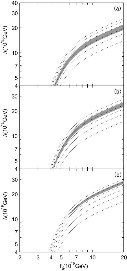
Figure 3: Constraint on the parameters $f_{\phi}$ and $\Lambda$. The shaded regions are for $\chi^{2}\leq 43$ for (a) $\tau=0$ (no reionization), (b) $\tau=0.2$, and (c) $\tau=0.4$. The dotted lines are contours of constant $\sigma_{8}$ (0.4, 0.6, 0.8, 1.0, 1.2, and 1.4, from below).

In Fig. 3, we show the constraint on the $f_{\phi}$ vs. $\Lambda$ plane. We shaded the region with $\chi^{2}\leq 43$ (which corresponds to 95 % C.L. allowed region for the $\chi^{2}$-statistics with 29 degrees of freedom). For a fixed $f_{\phi}$, we obtain upper and lower bounds on $\Lambda$. With $f_{\phi}$ being fixed, the primordial curvature perturbation is an increasing function of $\Lambda$, and hence $\Lambda$ is required to have a relevant value to explain the observed size of the multipoles. Notice that, for large enough $f_{\phi}$, the upper and lower bounds on $\Lambda$ are proportional to $f_{\phi}^{1/2}$. This is because the observable quantities depend only on $m_{\phi}=\Lambda^{2}/\sqrt{2}f_{\phi}$ in this region.

Now, let us comment on the case with $f_{\phi}\gg M_{*}$. In this case, the index $n_{\rm S}$ becomes close to 1 and the theoretical predictions on $\tilde{C}_{l}$ for $l\mathop{}_{\textstyle\sim}^{\textstyle>}400$ become larger than the observed ones. However, the asymptotic value of $n_{\rm S}$ for $f_{\phi}\gg M_{*}$ is 0.96, not exactly equal to 1. Thus, the constraints from the multipoles around the second peak is not as severe as those for models with the scale-invariant Harrison-Zeldovich spectrum. In addition, since we used all the data points to evaluate $\chi^{2}$ and required $\chi^{2}\leq 43$, the discrepancies for $l\mathop{}_{\textstyle\sim}^{\textstyle>}400$ are not statistically significant enough to exclude the parameter region with $f_{\phi}\gg M_{*}$. Thus, in Fig. 3, no upper bound on $f_{\phi}$ is obtained. However, it is interesting to consider the constraint from the second peak. As an example, following Ref. [9], we identified the highest data points for $l<400$ and $400\leq l\leq 600$ as the heights of the first and second peaks, $\tilde{C}_{l}^{\rm 1st}$ and $\tilde{C}_{l}^{\rm 2nd}$, respectively. Then, we combined the two data samples from BOOMERANG and MAXIMA to obtain

$$\tilde{C}_{l}^{\rm 2nd}/\tilde{C}_{l}^{\rm 1st}=0.38\pm 0.06.$$ (23)

Requiring $\tilde{C}_{l}^{\rm 2nd}/\tilde{C}_{l}^{\rm 1st}\leq 0.50$, we obtain $f_{\phi}\mathop{}_{\textstyle\sim}^{\textstyle<}7\times 10^{18}\ {\rm GeV}$. In the future, more accurate measurements of the CMBR anisotropy will be able to check the validity of this upper bound.

Another independent constraint is available from the cluster abundance. In Fig. 3, we plotted the contours of the constant $\sigma_{8}$, where $\sigma_{8}$ is the amplitude of mass density fluctuations on the scale of $8h^{-1}\ {\rm Mpc}$. The observed value of $\sigma_{8}$ is given by $\sigma_{8}=(0.56\pm 0.06)\Omega_{0}^{-0.47}$ [21]. As one can see, in case without reionization, $\sigma_{8}$ is consistent with the above-mentioned value in the parameter region preferred by the CMBR anisotropy.

So far, we have not discussed the effect of the reionization after the recombination. Its effect is well parameterized by the following two parameters: the optical depth $\tau$ and the red shift $z_{\rm ion}$ at the time of the reionization [23, 24]. Due to the reionization, $\tilde{C}_{l}$’s with $l\gg z_{\rm ion}^{1/2}$ are suppressed by the factor $e^{-2\tau}$ while those with small $l$ are unchanged. We calculated $\chi^{2}$ with the reionization with $\tau=0.2$ and $0.4$. For a fixed value of $\tau$, we took several values of $z_{\rm ion}$ of $O(10)$, and checked that $\chi^{2}$ is almost independent of $z_{\rm ion}$. The results are shown in Fig. 3. Since the reionization effect reduces $\tilde{C}_{l}$, larger value of the primordial perturbation is needed to obtain the CMBR anisotropy consistent with the observations. Thus, the preferred value of $\Lambda$ becomes larger as $\tau$ increases, as shown in Fig. 3. In addition, when $\tau=0$ and $n_{\rm S}=1$, theoretical prediction for $\tilde{C}_{l}$ with $l\mathop{}_{\textstyle\sim}^{\textstyle>}400$ becomes larger than observations if we adopt the primordial curvature perturbation suggested by COBE. In this case, CMBR anisotropy prefers a index $n_{\rm S}$ smaller than 1. However, if the reionozatoin effect is sufficient, it suppresses $\tilde{C}_{l}$ with large $l$ and $n_{\rm S}<1$ makes the fit worse. Thus, for large $\tau$, parameter region with small $f_{\phi}$, where $n_{\rm S}$ becomes significantly smaller than 1, is excluded. In addition, consistency with the constraint from the cluster abundance becomes worse for larger $\tau$, as shown in Fig. 3.

Finally, we briefly discuss possible improvement of the constraints with future observations. With MAP [25] and PLANCK [26] experiments, much better observations of the CMBR anisotropy will be obtained. It has been pointed out that MAP and PLANCK will determine the index $n_{\rm S}$ with $O(1\ \%)$ accuracy [27]. In the natural inflation model, $n_{\rm S}$ is sensitive to $f_{\phi}$. For example, $5.2\times 10^{18}\ {\rm GeV}\leq f_{\phi}\leq 5.7\times 10^{18}\ {\rm GeV}$ gives $0.89\leq n_{\rm S}\leq 0.91$. In addition, $C_{l}$ itself will be determined much more accurately, and hence the theoretical prediction on the CMBR anisotropy will be more directly compared with the observation. Thus MAP and PLANCK will provide much better constraint on the natural inflation model than the present one.

Acknowledgment: One of the authors (TM) would like to thank T. Asaka and Y. Nomura for useful conversations. This work is supported by the Grant-in-Aid for Scientific Research from the Ministry of Education, Science, Sports, and Culture of Japan (No. 12047201).

References

- [1] A.H. Guth, Phys. Rev. D23 (1981) 347.
- [2] A.D. Linde, Phys. Lett. B108 (1982) 389.
- [3] A. Albrecht and P.J. Steinhardt, Phys. Rev. Lett. 48 (1982) 1220.
- [4] K. Freese, J.A. Frieman and A.V. Olinto, Phys. Rev. Lett. 65 (1990) 3233.
- [5] F.C. Adams, J.R. Bond, K. Freese, J.A. Frieman and A.V. Olinto, Phys. Rev. D47 (1993) 426.
- [6] P. de Bernardis et al., Nature 404 (2000) 955.
- [7] S. Hanany et al., astro-ph/0005123.
- [8] W.H. Kinney, A. Melchiorri and A. Riotto, astro-ph/0007375.
- [9] L. Covi and D. Lyth, astro-ph/0008165.
- [10] See, for example, D.H. Lyth and A. Riotto, Phys. Rept. 314 (1999) 1.
- [11] See, for example, E.W. Kolb and M.S. Turner, “The Early Universe” (Addison-Wesley, 1990).
- [12] S.M. Carroll, W. Press and E.L. Turner, Annu. Rev. Astron. Astrophys. 30 (1992) 499.
- [13] C.L. Bennett et al., Astrophys. J. 464 (1996) L1.
- [14] E.F. Bunn and M. White, Astrophys. J. 480 (1997) 6.
- [15] See, for example, W. Hu, Ph. D Thesis (astro-ph/9508126).
- [16] U. Seljak and M. Zaldarriaga, “CMBFAST: A Microwave Anisotropy Code” (http://www.sns.ias.edu/∼matiasz/CMBFAST/cmbfast.html).
- [17] J.R. Primack, astro-ph/0007187.
- [18] M.S. Turner, astro-ph/9904051.
- [19] M. Tegmark and A.J.S. Hamilton, astro-ph/9702019.
- [20] A.H. Jaffe et al., astro-ph/0007333.
- [21] P.T.P. Viana and A.R. Liddle, astro-ph/9902245.
- [22] S.D. White, G. Efstathiou and C.S. Frenk, Mon. Not. Roy. Astron. Soc. 262 (1993) 1023.
- [23] W. Hu and M. White, Astrophys. J. 479 (1997) 568.
- [24] L.M. Griffiths, D. Barbosa and A.R. Liddle, astro-ph/9812125.
- [25] MAP home page (http://map.gsfc.nasa.gov/).
- [26] PLANCK home page (http://astro.estec.esa.nl/SA-general/Projects/Planck).
- [27] J.R. Bond, G. Efstathiou and M. Tegmark, Mon. Not. Roy. Astron. Soc. 291 (1997) L33.