Semileptonic form factors – a model-independent approach

Abstract

We demonstrate that the $B\rightarrow D^{(*)}l\nu$ form factors can be accurately predicted given the slope parameter $\rho^{2}$ of the Isgur-Wise function. Only weak assumptions, consistent with lattice results, on the wavefunction for the light degrees of freedom are required to establish this result. We observe that the QCD and $\frac{1}{m_{Q}}$ corrections can be systematically represented by an effective Isgur-Wise function of shifted slope. This greatly simplifies the analysis of semileptonic $B$ decay. We also investigate what the available semileptonic data can tell us about lattice QCD and Heavy Quark Effective Theory. A rigorous identity relating the form factor slope difference $\rho_{D^{*}}^{2}-\rho_{A_{1}}^{2}$ to a combination of form factor intercepts is found. The identity provides a means of checking theoretically evaluated intercepts with experiment.

I Outline

We obtain a nearly model-independent description of the Isgur-Wise (IW) function [1], $\xi(w)$, in terms of a single measurable parameter — the slope at zero-recoil, $\rho^{2}$. Only modest assumptions about the shape of the heavy-light wavefuction are required, and these are consistent with an established lattice result. We obtain a simple functional form for the IW function in terms of $\rho^{2}$:

$$\xi(w,\rho^{2})=\frac{2(w+1)}{[w+1+(\rho^{2}-\frac{1}{2})(w-1)]^{2}}\,.$$ (1)

We also demonstrate that the effect of radiative QCD corrections and $\frac{1}{m}$ corrections can be described as the product of a term linear in $w$ and the IW function. The resulting function is also approximately an IW function of shifted slope. Thus, fitting the above functional form to the measured form factors provides an accurate description of the extrapolation to zero-recoil. Over the range of expected slopes, our result is in good agreement with the work of [3, 4, 5] which is based on dispersion relations.

Recent analyses [6, 7] of $B\rightarrow Dl\nu$ and $B\rightarrow D^{*}l\nu$ decays extract two physical form factors and two ratios of physical form factors. We show that this information can be directly related to QCD predictions.

In Section II we provide some background formalism behind form factors for semileptonic $B$-decay and the Isgur-Wise function. We present our description of the IW function in terms of the slope parameter, $\rho^{2}$, in Section III. In Section IV we discuss the effects of corrections to the heavy-quark limit and their equivalence to slope-shifted IW functions. The relationship of HQET and QCD lattice simulation to semileptonic data is explored in Section V.

II Introduction

As the observed sample of semileptonic $B$ decays accumulates, the need for a rigorous method of analysis becomes more pressing. Even in the heavy quark limit, a universal form factor is required for each light degree of freedom state of the meson. To compute the Isgur-Wise (IW) functions $\xi(w)$, where $w=v^{\mu}v_{\mu}^{\prime}$, requires considerable knowledge of the heavy-light meson dynamics. For this reason, the IW function is usually thought of as “model-dependent” and not susceptible to reliable calculation. In the first portion of this paper we seek a balance between rigorous constraints and phenomenological usefulness. We will demonstrate, from heavy quark symmetry and some qualitative lattice results, that the IW function is accurately determined by specifying only the slope parameter, $\rho^{2}$.

Experimentalists commonly adopt the straightforward procedure of expanding form factors about the meson zero-recoil point ($w=1$),

$$\xi(w)=1-\rho^{2}(w-1)+c(w-1)^{2}+\ldots$$ (2)

Burdman [8] has pointed out that the effect of the curvature term $c$ is significant but that, for statistical reasons, much predictive power is lost when it is a free parameter. A “model-independent” relation between $c$ and the slope parameter $\rho^{2}$ has been proposed by Boyd, Grinstein and Lebed [2]. This method has been modified by Caprini and Neubert [3] and by Caprini, Lellouch, and Neubert in expanded form [4]. This result has been criticized however by Boyd, Grinstein, and Lebed [5]. These latter authors propose a similar but weaker relation between $c$ and $\rho^{2}$. In Section III, we propose a rigorous one-parameter expression for the IW function.

The second observation we make here concerns the relation of the IW function to the actual (physical) form factors with $\frac{1}{m_{Q}}$ and QCD radiative corrections. We show in section IV that all of these corrections can be distilled into a new effective IW function with a shift in slope. The analysis of experimental data is thereby greatly simplified. The slopes appearing in $B\rightarrow D$ and $B\rightarrow D^{*}$ will be different and this difference can be compared to the theoretical predictions.

The decay rate for $B\rightarrow D^{(*)}l\bar{\nu}$ can be written [9] as,

$$\frac{d\Gamma}{dw}=\frac{G_{F}^{2}|V_{cb}|^{2}}{48\pi^{3}}m_{B}^{2}m_{D^{(*)}}^{3}\sqrt{w^{2}-1}f^{(*)}|F^{(*)}|^{2}\,,$$ (3)

where for $B\rightarrow Dl\bar{\nu}$

$\displaystyle f=(w^{2}-1)(1-r)^{2}\,,$

$$r=\frac{m_{D}}{m_{B}}\approx 0.35\,,$$ (4)

and for $B\rightarrow D^{*}l\bar{\nu}$

$\displaystyle f^{*}=(w+1)[(w+1)(1-r^{*})^{2}+4w(1-2wr^{*}+r^{*2})]\;,$

$$r^{*}=\frac{m_{D^{*}}}{m_{B}}\approx 0.38\;.$$ (5)

The two form factors $F(w)$ and $F^{*}(w)$ can be expressed [10] in terms of the fundamental form factors $h_{+}$, $h_{-}$, $h_{V}$, $h_{A_{1}}$, $h_{A_{2}}$, and $h_{A_{3}}$. These form factors can in turn be related to the Isgur-Wise function through

$$h_{i}(w)=[\alpha_{i}+\beta_{i}(w)+\gamma_{i}(w)]\xi(w)\;.$$ (6)

where $\alpha_{+}=\alpha_{V}=\alpha_{A_{1}}=\alpha_{A_{3}}=1$ and $\alpha_{-}=\alpha_{A_{2}}=0$. The $\beta_{i}(w)$ describe perturbative radiative corrections and are in principle predictable within the heavy quark effective theory. The $\gamma_{i}(w)$ represent the power ($\frac{1}{m_{Q}}$) deviations from heavy quark symmetry and require further theoretical assumptions [10]. In Section IV we will point out that, for those form factors which do not vanish in the heavy quark limit, the pre-factors in (6) can nevertheless be approximately absorbed into an effective IW function which has a flavor and spin-dependent slope

$$h_{i}(w)\simeq h_{i}(1)\xi(w,\rho_{i}^{2})$$ (7)

III Model independent parametrization of the Isgur-Wise function

The IW function appears to require detailed information on the nature of heavy-light dynamics. In this section, we propose a method to distill most of this knowledge into a single parameter — the slope $\rho^{2}$. Almost all model dependence will be seen to vanish once the slope is specified.

In the heavy-light limit, heavy quark symmetry provides a unique prescription [11, 12] relating the IW function to the wavefunction and light degrees of freedom energy E,

$$\xi(w)=\frac{2}{w+1}\left<j_{0}\Bigl{(}2Er\sqrt{\frac{w-1}{w+1}}\Bigr{)}\right>\,.$$ (8)

The expectation value may involve a multi-component wavefunction such as from the Dirac equation. For simplicity of notation, we assume a single component wavefunction $\psi(\mbox{$\bf{r}$})=R(r)Y_{l}^{m}(\theta,\phi)$. The expectation value is consequently defined by

$$\left<A(r)\right>\equiv\int\limits_{0}^{\infty}dr\>r^{2}R^{2}(r)A(r)\,.$$ (9)

Using $\lim_{y\ll 1}j_{0}(y)=1-\frac{1}{6}y^{2}+\ldots\,$, we may expand (8) about the zero recoil point $w=1$ to yield:

$$\xi(w) \approx [1-\frac{1}{2}(w-1)+\ldots][<\!1\!>-\frac{4E^{2}}{6}(\frac{w-1}{w+1})<\!r^{2}\!>+\ldots]$$ (10)

$$\xi(w) \approx 1-\rho^{2}(w-1)+\ldots$$ (11)

where

$$\rho^{2}=\frac{1}{2}+\frac{E^{2}}{3}\left<r^{2}\right>\;.$$ (12)

We now use (12) to eliminate the energy $E$ in the general expression (8) to obtain:

$$\xi(w)=\frac{2}{w+1}\biggl{<}j_{o}\Bigl{(}\frac{r}{r_{rms}}\sqrt{\frac{12(\rho^{2}-\frac{1}{2})(w-1)}{w+1}}\Bigr{)}\biggr{>}\;,$$ (13)

where $r_{rms}=\sqrt{\left<r^{2}\right>}$.

In the above (13), if we know the slope ($\rho^{2}$) and the radial ground state heavy quark wavefunction, we can compute the IW function for all $w$. We can make the wavefunction dependence more explicit by introducing the dimensionless quantities

$$x \equiv \frac{r}{r_{0}}\,,$$ (14)

$$R(r) = R_{0}f(\frac{r}{r_{0}})=R_{0}f(x)\,,$$ (15)

where $r_{0}$ is a hadronic scale factor. We define the $n^{th}$ moment of $f^{2}$ as

$$N_{n}\equiv\int\limits_{0}^{\infty}dx\>x^{n+2}f^{2}(x)$$ (16)

so that wave function normalization and $\left<r^{2}\right>$ become:

$$r_{0}^{3}R_{0}^{2}N_{0} = 1\,,$$ (17)

$$<\!r^{2}\!> = r_{0}^{5}R_{0}^{2}N_{2}=r_{0}^{2}\frac{N_{2}}{N_{0}}\,.$$ (18)

The IW function (13) is then

$$\xi(w)=\frac{2}{w+1}\frac{1}{N_{0}}\int\limits_{0}^{\infty}dx\>x^{2}f^{2}(x)j_{0}\biggl{(}x\sqrt{\frac{12(\rho^{2}-\frac{1}{2})(w-1)N_{0}}{(w+1)N_{2}}}\biggr{)}\,.$$ (19)

It should be noted that both the normalization constant $R_{0}$ and the hadronic scale parameter $r_{0}$ do not appear in the above expression for the IW function. The IW function thus depends only on the dimensionless slope parameter $\rho^{2}$ and one dimensionless function $f(x)$ which is essentially the heavy-light wavefunction.

A few years ago, the heavy-light wavefunction was evaluated in quenched lattice simulation [13]. The result for the ground state is shown in Fig. 1. One may observe that the lattice wavefunction closely resembles a simple exponential. We use this lattice result as a guide and parametrize the wavefunction as [14]:

$$f(x)=e^{-x^{k}}\,.$$ (20)

When $k=1$ the wavefunction is a simple exponential and the lattice simulation is closely reproduced. In Fig. 1, we also show that by choosing $k=0.5$ and $k=2$ we very conservatively bracket the observed wavefunction. Assuming the heavy-light wavefunction is given by (20) with

$$0.5\leq k\leq 2\,,$$ (21)

the IW function is determined for all $w$ once the slope is specified. In Fig. 2 we show the predicted IW function with $\rho^{2}=0.9$. The central curve corresponds to $k=1$ with a corridor implied by the limits of (21). We note that at $w=1.5$, which is approximately the largest allowed for $B\rightarrow D^{(*)}l\nu$ decay, the corridor width is only about 0.02, or 3%. This small uncertainty shows that most of the IW shape is well-determined by the slope alone.

A particularly important special case is when $k=1$. Straightforward evaluation of (19) with $k=1$ in (20) yields the IW function

$$\xi(w,\rho^{2})=\frac{2(w+1)}{[w+1+(\rho^{2}-\frac{1}{2})(w-1)]^{2}}\;.$$ (22)

The above Isgur-Wise function will be accurate within the corridor shown in Fig. 2.

IV The Physical Form Factors

An important observation from specific theoretical models [15] is that the subleading Isgur-Wise form factors which characterize the $\frac{1}{m_{Q}}$ corrections are to a good approximation linear in $w$. In addition, the radiative QCD corrections are monotonic and vary slowly with $w$, so that they too can be approximated linearly. Hence each of the $h_{i}(w)$ form factors (6) can be written as

$$h_{i}(w)\simeq[\alpha_{i}+\lambda_{i}+\mu_{i}(w-1)]\xi(w)\,,$$ (23)

where both $\lambda_{i}$ and $\mu_{i}$ are small, dimensionless constants. The advantage of this observation is that an analysis of the experimental form factor can now be carried out without a priori knowledge of the ${\lambda_{i}}$ and ${\mu_{i}}$ coefficients.

To take advantage of the above, we start with the expansion (10) and note that for small $(w-1)$, IW functions of slopes $\rho^{2}+\Delta\rho^{2}$ and $\rho^{2}$ are related by

$$\xi(w,\rho^{2}+\Delta\rho^{2})\simeq\xi(w,\rho^{2})-\Delta\rho^{2}(w-1)\,.$$ (24)

Over a wider range of $w$ a more accurate expansion is

$$\xi(w,\rho^{2}+\Delta\rho^{2})\simeq\xi(w,\rho^{2})[1-\Delta\rho^{2}(w-1)]\,.$$ (25)

To illustrate the above approximation, we show in Fig. 3 a simple physical form factor (with $\mu=0.1$),

$$h(w)=\xi(w,1.0)[1+0.1(w-1)]\;.$$ (26)

Also on Fig. 3 is a shifted IW function $\xi(w,0.9)$ with slope chosen by the above prescription. We note that the two form factors differ by less than 2% at $w=1.5$. We now apply this result to the form factors $h_{i}(w)$. Comparing (25) to (23) in the case where $\alpha_{i}=1$ we see that

$$h_{i}(w) \simeq \xi(w,\rho^{2}+\Delta\rho^{2})+\lambda_{i}\xi(w,\rho^{2})\;,$$ (27)

$$\simeq \xi(w,\rho^{2}+\Delta\rho^{2})+\lambda_{i}\xi(w,\rho^{2}+\Delta\rho^{2})[1+\Delta\rho^{2}(w-1)];.$$ (28)

We drop the small product $\lambda_{i}\Delta\rho^{2}$ to obtain

$$h_{i}(w)\simeq h_{i}(1)\xi(w,\rho_{i}^{2})\;,$$ (29)

with

$$\rho_{i}^{2} = \rho^{2}-\mu_{i}\;,$$ (30)

$$h_{i}(1) = 1+\lambda_{i}\;.$$ (31)

We may therefore conclude that the physical form factors are nearly equivalent to IW form factors with shifted slopes and normalizations.

As pointed out by Neubert [4, 15], the sub-leading from factor $\chi_{1}$ contributes identically to all of the $h_{i}$ which remain in the heavy quark limit. We therefore simplify the analysis by absorbing this $\chi_{1}$ contribution into a new IW type function which maintains spin-symmetry, but now has flavor dependence. It is this slope $\rho^{2}$ which we refer to as the IW slope in the following.

The absorption of $\chi_{1}$ into the IW function is allowed as long as $\chi_{1}$ remains small. The evidence for this is ambiguous. A QCD sum rule evaluation [15] gives a wide range of possible values for $\chi_{1}$, some of which are large. Evidence that $\chi_{1}$ is small comes, indirectly, from the dispersive analysis of Caprini, Lellouch and Neubert [4] where the $B\rightarrow Dl\nu$ is found for a given slope. In Fig. 4 we show the CLN prediction for $\rho^{2}=1$ compared to our $k=1$ prediction (22) for the same slope. The two curves are nearly identical, which is expected if $\chi_{1}$ and other corrections are small and can be absorbed into an effective IW function.

V What Can We Learn from Experimental Form Factors?

The semileptonic $B$ decays yield definite but limited information about QCD corrections. It is important to understand exactly what in a theoretical framework is being tested by experiment. In this section, we examine each observable quantity to see which aspect of QCD is being tested. We consider the semileptonic decays separately.

A  $B\rightarrow Dl\nu$

For $B\rightarrow Dl\bar{\nu}$, the form factor is [4]

$$F(w)\equiv V_{1}(w) = h_{+}(w)+\frac{1-r}{1+r}h_{-}(w)$$ (32)

$$= \xi(w,\rho^{2})[1+\lambda_{D}+\mu_{D}(w-1)+\ldots]$$ (33)

where

$$\lambda_{D} = \lambda_{h_{+}}+\frac{1-r}{1+r}\lambda_{h_{-}}$$ (34)

$$\mu_{D} = \mu_{h_{+}}+\frac{1-r}{1+r}\mu_{h_{-}}$$ (35)

and hence

$$\rho^{2}_{D}=\rho^{2}-\mu_{D}\,.$$ (36)

The only measurable parameter here is the physical form factor slope, $\rho_{D}^{2}$, which has been investigated at CLEO [7]. If the data improves sufficiently, the difference between $\rho_{D}^{2}$ and the slope of a different physical form factor (such as $F^{*}$) could provide information about QCD. To gain a rough idea of the sizes of $\lambda_{D}$ and $\mu_{D}$ we compute the Wilson coefficients and substitute the QCD sum rule approximations for the actual values of the subleading IW form factors. The results are included in the Table II of Appendix A.

There are some directly applicable tests of HQET provided by QCD lattice simulations. Accurate lattice simulations are currently possible at the zero recoil point ($w=1$). A recent calculation [16] obtains:

$$\lambda_{h_{+}} = \phantom{+}0.01\;,$$ (37)

$$\lambda_{h_{-}} = -0.11\;.$$ (38)

In HQET, these coefficients are due to the radiative corrections and $1/m$ corrections [4]. These are enumerated in Appendix A. We observe that $\lambda_{h_{+}}$ has no $1/m$ corrections as required by Luke’s Theorem [17]. The result from the Wilson coefficients alone of $\lambda_{h_{+}}=0.02$ is consistent with the lattice result (37).

The comparison with $\lambda_{h_{-}}$ of (38) is more interesting. The $1/m$ correction here contains the subleading form factor $\eta$. This form factor has been estimated by QCD sum rules [18], by ISGW2 [19], and by a Salpeter equation method [20]. While these various calculations yield reasonably consistent results for the subleading form factor $\chi_{2}(w)$, the expectations for $\eta(w)$ vary widely. From Appendix A we see that

$$\lambda_{h_{-}}=h_{-}(1)=(C_{2}-C_{3})+\left(\frac{1}{2m_{b}}+\frac{1}{2m_{c}}\right)(2\eta-1)\bar{\Lambda}\,.$$ (39)

Using the calculated Wilson coefficients and the parameters $m_{b}=4.80$ GeV, $m_{c}=1.45$ GeV, and $\bar{\Lambda}=0.5$ GeV we can evaluate the previous expression to yield

$$\lambda_{h_{-}}=-0.07+0.12(2\eta-1)\,.$$ (40)

The lattice result in (38) suggests that the second term above is negative, i.e. $\eta<0.5$. This prediction is not completely rigorous as the size of the effect is of order a few percent and second-order $1/m$ corrections could be of that order. In addition, the lattice calculation for $h_{-}(1)$ has currently been calculated only to tree level, but a 1-loop calculation is underway [16]. However, the preliminary indication is that $\eta$ is less than the central value of 0.62 which comes from QCD sum rules. At the same time however, the much smaller values of $\eta$ which come from ISGW2 and the Salpeter model are also disfavored because they produce a result for $h_{-}(1)$ which is too negative.

B  $B\rightarrow D^{*}l\nu$

In this case, there is additional information provided by the $D^{*}\rightarrow D\pi$ decay distribution [6]. As suggested by CLN [4] and followed by CLEO [6] this decay can be analyzed in terms of the $h_{A_{1}}$ form factor and two ratios of form factors.

The CLEO experiment, which to date has the best measurements of the $B\rightarrow D^{*}$ form factor paramaters, has adopted the convention of fitting the slope of $h_{A_{1}}$, $\rho^{2}_{A_{1}}$ and two form factor ratios:

$$R_{1}(w) = \frac{h_{V}(w)}{h_{A_{1}}(w)}\,,$$ (41)

$$R_{2}(w) = \frac{h_{A_{3}}(w)+r^{*}h_{A_{2}}(w)}{h_{A_{1}}(w)}\,,$$ (42)

where $r^{*}=\frac{m_{D^{*}}}{m_{B}}\approx 0.38$. These ratios are expected to be nearly independent of $w$ so they are treated as constants in the fit. The form factor $F^{*}$ can be expressed in terms of these parameters by combining Equation (A6) from Appendix A and the definitions (42). We would also like to write $F^{*}(w)$ as a shifted IW function,

$$F^{*}(w)=\xi(w,\rho^{2})[1+\lambda_{D^{*}}+\mu_{D^{*}}(w-1)+\ldots]\;,$$ (43)

and hence

$$F^{*}(w)=F^{*}(1)\xi(w,\rho_{D^{*}}^{2})\,,$$ (44)

where $\rho_{D^{*}}^{2}=\rho^{2}-\mu_{D^{*}}$. Since $|F^{*}|^{2}$ is the sum of $h_{i}$ contributions and kinematical factors, the $\lambda_{D^{*}}$ and $\mu_{D^{*}}$ are the result of an expansion about $w=1$. The result is

$$\lambda_{D^{*}} = \lambda_{A_{1}}\,,$$ (45)

$$\mu_{D^{*}} = \mu_{A_{1}}+\frac{1}{3}\lambda_{V}-\frac{1}{3(1-r^{*})}[\lambda_{A_{3}}+r^{*}\lambda_{A_{2}}-r^{*}\lambda_{A_{1}}]\,.$$ (46)

As in the $B\rightarrow Dl\nu$ case, we can obtain rough approximations of $\mu_{D^{*}}$, $\lambda_{D^{*}}$, $\mu_{A_{1}}$ and $\lambda_{A_{1}}$. The results are included in Table II of Appendix A.

The above expression (46) has a remarkable consequence. The slope difference $\rho_{D^{*}}^{2}-\rho^{2}_{A_{1}}=\mu_{A_{1}}-\mu_{D^{*}}$ can be related to the zero-recoil quantities, $\lambda_{i}$ above. It is therefore possible in the near future to test (for the first time) the “intercept” quantities $\lambda_{i}$ by direct comparison to experiment. At this point only $\lambda_{A_{1}}$ has been computed in lattice simulation [21], but the corresponding values of $\lambda_{A_{2}}$, $\lambda_{A_{3}}$, and $\lambda_{V}$ could be evaluated. At present the experimental situation [6] is also not precise enough:

$$\rho^{2}_{D^{*}}-\rho^{2}_{A_{1}}=0.08\pm 0.15\,,$$ (47)

but this result can also be considerably sharpened. We emphasize that the above prediction (46) is an important check of the values of the intercepts, $\lambda_{i}$, which are in turn of critical importance in the extraction of the CKM parameter $V_{cb}$.

In the heavy quark limit, $R_{1}=R_{2}=1$. These ratios’ deviation from unity, experimentally and theoretically, indicates deviation from heavy quark symmetry and, consequently, can test theoretical predictions for the symmetry-breaking corrections. The measurements of $R_{1}$ and $R_{2}$ (currently with large error bars) agree with theoretical predictions, and thus roughly confirm the predictions of HQET. Here we investigate the exact nature of the predictions and their value as tests of HQET.

Treating the form factor ratios as constants, while reasonable theoretically and necessary for the fit, makes the tests of symmetry-breaking corrections less informative. $R_{1}(w)$ and $R_{2}(w)$ are essentially reduced to $R_{1}(1)$ and $R_{2}(1)$, and because many of the corrections vanish at $w=1$, they cannot be tested. For example, the subleading Isgur-Wise function $\chi_{3}(w)$ which has only been calculated up to the errors inherent to QCD sum rules is completely lost in this procedure. If we apply the expressions given in Appendix A to the various form factors at $w=1$, eliminate those corrections which vanish at zero-recoil, and express the results in terms of the Wilson coefficients and subleading IW form factors, we obtain:

$$R_{1}(1) = \frac{C_{1}(1)+\frac{1}{2m_{c}}\bar{\Lambda}-\frac{1}{2m_{b}}(2\eta-1)\bar{\Lambda}}{C_{1}^{5}(1)}$$ (48)

$$R_{2}(1) = \frac{C_{1}^{5}(1)+C_{2}^{5}(1)+r^{*}C_{2}^{5}(1)-\eta\bar{\Lambda}[\frac{1}{m_{b}}+\frac{(1+r^{*})}{2m_{c}}]+\frac{4\chi_{2}(1)}{2m_{c}}(r^{*}-1)+\bar{\Lambda}(\frac{1}{2m_{b}}-\frac{r^{*}}{2m_{c}})}{C_{1}^{5}(1)}$$ (49)

If we use the theoretical estimates as rough guides to the size of each term, we can determine what predictions are actually being tested.

1 What Do We Learn From $R_{1}$?

The subleading combination $2\eta-1$ is expected to be small on the basis of the $\lambda_{h_{-}}$ considerations and is further reduced by $\frac{1}{m_{b}}$. Consequently, after evaluating the Wilson coefficients $C_{i}$ (see Table I of Appendix A), $R_{1}$ must be greater than unity and provides a fairly direct probe of the HQET parameter $\bar{\Lambda}$, which is the light degrees of freedom energy to this order.

2 What Do We Learn From $R_{2}$?

In the expression for $R_{2}$, $\chi_{2}$ is generally agreed to be quite small and $\frac{1}{2m_{b}}-\frac{r^{*}}{2m_{c}}\approx 0.03$. Thus after calculating the Wilson coefficients, a measurement of $R_{2}$ provides an additional probe of the value of the subleading form factor $\eta$. Using the Wilson coefficients in Appendix A, as well as $m_{b}=4.8$ GeV, $m_{c}=1.45$ GeV, $r^{*}=0.38$ and $\bar{\Lambda}=0.5$ GeV, the expression for $R_{2}$ becomes

$$R_{2}=1.00-0.34\eta(1)-0.84\chi_{2}(1)\,.$$ (50)

The term containing $\eta$ is the dominant correction as $\chi_{2}$ is small, so a precise measurement of $R_{2}$ effectively measures $\eta$.

VI Conclusions

We have addressed the question of how to analyze semileptonic $B$ decay while minimizing both the amount of theoretical assumption and the number of parameters. We first establish that specifying the slope parameter $\rho^{2}$ accurately determines the entire Isgur-Wise function. To do so, we need only an approximation to the light degrees of freedom wavefunction provided by a QCD simulation. Our result (1) is

$$\xi(w,\rho^{2})=\frac{2(w+1)}{[w+1+(\rho^{2}-\frac{1}{2})(w-1)]^{2}}\;.$$ (51)

The form factors $h_{i}(w)$ either vanish or approach the IW function in the heavy quark limit. These amplitudes can be accurately written as

$$h_{i}(w)=[\alpha_{i}+\lambda_{i}+\mu_{i}(w-1)+\ldots]\xi(w,\rho^{2})\,,$$ (52)

where $\alpha_{i}$ is 0 or 1 and $\lambda_{i}$ and $\mu_{i}$ are small dimensionless constants. We observe that by altering the IW slope $\rho^{2}$ to $\rho_{i}^{2}=\rho^{2}-\mu_{i}$ the physical form factors can be expressed as

$$h_{i}(w)=(\alpha_{i}+\lambda_{i})\xi(w,\rho_{i}^{2})\,,$$ (53)

where $\rho_{i}^{2}=\rho^{2}-\mu_{i}$. That this works well is shown by Fig. 3.

From the above we conclude that semileptonic data are parametrized by an intercept value $V_{cb}(1+\lambda_{i})$ and an effective Isgur-Wise slope parameter $\rho_{i}^{2}$. To find the CKM element $V_{cb}$ one must use a theoretical estimate of $\lambda_{i}$.

For $B\rightarrow D^{*}l\nu$ decay the parameters are $V_{cb}(1+\lambda_{A_{1}})$, $\rho_{A_{1}}^{2}$, $R_{1}$, and $R_{2}$. In this case one has a consistency condition (46) relating the $\lambda_{i}$ and the difference between actual $D^{*}$ slope and $\rho^{2}_{A_{1}}$. We further point out that $R_{1}$ is nearly model-independent while $R_{2}$ depends sensitively on various estimates of the subleading from factor $\eta(1)$. Also, the value of the form factor $h_{-}(w)$ at zero-recoil, $\lambda_{h_{-}}$, appears to offer an additional probe of the value $\eta(1)$.

Finally, one might ask, what is the essential advantage of the slope shift scheme described here? The answer is, economy of parameters and a decoupling from theoretical assumptions. As seen in Fig. 3, one of the effective IW function slopes is equivalent to an (unknown) IW slope with subleading corrections. If these corrections were securely known our scheme offers no advantage. On the other hand, if one tried to fit both the IW slope and HQET $\mu$ parameters, a hopeless parameter correlation would arise.

We believe that it is best to rely as little as possible on theory and to use a direct phenomenological approach. As pointed out previously[8], one must have some theoretical constraint on the curvature term in (2). We show here that the shape of the form factor is specified once the slope parameter is given. Later, after the decay distributions have been parametrized, the fitted parameters can be compared to predictions.

A

The fundamental form factors $h_{i}$ are defined [4, 10] by

$$\frac{\langle D(v^{\prime})|\bar{c}\gamma^{\mu}b|B(v)\rangle}{\sqrt{m_{B}m_{D}}} = (v+v^{\prime})^{\mu}h_{+}(w)+(v-v^{\prime})^{\mu}h_{-}(w),$$ (A1)

$$\frac{\langle D^{*}(v^{\prime},\epsilon)|\bar{c}\gamma^{\mu}b|B(v)\rangle}{\sqrt{m_{B}m_{D^{*}}}} = i\epsilon^{\mu\nu\alpha\beta}\epsilon^{*}_{\nu}v_{\alpha}^{\prime}v_{\beta}h_{V}(w),$$ (A2)

$$\frac{\langle D^{*}(v^{\prime},\epsilon)|\bar{c}\gamma^{\mu}\gamma^{5}b|B(v)\rangle}{\sqrt{m_{B}m_{D^{*}}}} = (w+1)\epsilon^{*\mu}h_{A_{1}}(w)-\epsilon^{*}\cdot v(v^{\mu}h_{A_{2}}+v^{\prime\mu}h_{A_{3}})$$ (A3)

The matrix elements for $B\rightarrow Dl\bar{\nu}$ in (5) can be expressed in terms of {$h_{i}$} as

$$F(w)=h_{+}(w)-\biggl{(}\frac{1-r}{1+r}\biggr{)}h_{-}(w)$$ (A4)

and the squared matrix element for $B\rightarrow D^{*}l\bar{\nu}$ in (5) as

$$f^{*}|F^{*}(w)|^{2} = 2(w+1)(1-2wr^{*}+r^{*2})[(w+1)h_{A_{1}}^{2}+(w-1)h_{V}^{2}]$$ (A6)

$$+(w+1)^{2}[(w-r^{*})h_{A_{1}}-(w-1)(r^{*}h_{A_{2}}+h_{A_{3}})]^{2}\,.$$

The $h_{i}$ can, as indicated in (6), be expressed by the short-range corrections $\beta_{i}$ and the $\frac{1}{m_{Q}}$ corrections $\gamma_{i}$ together as

$$h_{V}(w) = \xi(w)[C_{1}+\varepsilon_{c}(L_{2}-L_{5})+\varepsilon_{b}(L_{1}-L_{4})]$$ (A7)

$$h_{A_{3}}(w) = \xi(w)[C_{1}^{5}+C_{3}^{5}+\varepsilon_{c}(L_{2}-L_{3}-L_{5}+L_{6})+\varepsilon_{b}(L_{1}-L_{4})]$$ (A8)

$$h_{A_{2}}(w) = \xi(w)[C_{2}^{5}+\varepsilon_{c}(L_{3}+L_{6})]$$ (A9)

$$h_{A_{1}}(w) = \xi(w)[C_{1}^{5}+\varepsilon_{c}(L_{2}-\frac{w-1}{w+1}L_{5})+\varepsilon_{b}(L_{1}-\frac{w-1}{w+1}L_{4})]$$ (A10)

$$h_{+}(w) = \xi(w)[C_{1}+\frac{w+1}{2}(C_{2}+C_{3})+(\varepsilon_{c}+\varepsilon_{b})L_{1}]$$ (A11)

$$h_{-}(w) = \xi(w)[\frac{w+1}{2}(C_{2}-C_{3})+(\varepsilon_{c}+\varepsilon_{b})L_{4}]$$ (A12)

where $\varepsilon_{c,b}=(2m_{c,b})^{-1}$, the $C_{i}$ are the Wilson coefficients — which are discussed extensively in [15] — and the $L_{i}$ are combinations of the sub-leading Isgur Wise form factors and have been approximated by QCD sum rules [4]:

$$L_{1} = -4(w-1)\frac{\chi_{2}}{\xi}+12\frac{\chi_{3}}{\xi}\approx 0.72(w-1)\bar{\Lambda}$$ (A13)

$$L_{2} = -4\frac{\chi_{3}}{\xi}\approx-0.16(w-1)\bar{\Lambda}$$ (A14)

$$L_{3} = 4\frac{\chi_{2}}{\xi}\approx 0.24\bar{\Lambda}$$ (A15)

$$L_{4} = (2\eta-1)\bar{\Lambda}\approx 0.24\bar{\Lambda}$$ (A16)

$$L_{5} = -\bar{\Lambda}$$ (A17)

$$L_{6} = -\frac{2}{w+1}(\eta+1)\bar{\Lambda}\approx-\frac{3.24}{w+1}\bar{\Lambda}$$ (A18)

where $\bar{\Lambda}\approx 0.5~{}\rm{GeV}$ is the “binding energy” of a heavy meson.

Using the detailed expressions given in [4] and [15] and the expressions above, we can extract $\lambda_{i}$ and $\mu_{i}$ for each form factor $h_{i}$ which appears in (23). They appear in the following table. We use the values $m_{b}=4.8~{}\rm{GeV}$ and $m_{c}=1.45~{}\rm{GeV}$ and calculate the Wilson coefficients at the scale $\alpha_{s}(\mu)=0.12\pi$.

TABLE I.: Wilson coefficient linear fits for $\alpha(\mu)=0.12\pi$ [15].

$C_{i}$	$C_{i}(1)$	$C_{i}^{\prime}(1)$
$C_{1}$	1.13	$-0.08$
$C_{1}^{5}$	1.00	$-0.04$
$C_{2}$	$-0.086$	0.037
$C_{2}^{5}$	$-0.11$	0.038
$C_{3}$	$-0.019$	0.005
$C_{3}^{5}$	0.040	$-0.013$

TABLE II.: Estimates of the $\lambda$ and $\mu$ coefficients for the various relevant form factors using the Wilson coefficients of Table I and QCD sum rules[4, 18] as summarized in the Appendix.

Form Factor	$\lambda_{i}$	$\mu_{i}$
$h_{A_{1}}$	0.004	0.050
$F_{D}=V_{1}$	0.041	0.072
$F^{*}={\cal F}$	0.004	0.253

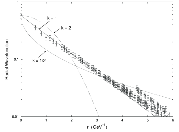
FIG. 1.: The lattice data [13] for the heavy-light wavefunction along with curves corresponding to the exponential parametrization (20) with $k=0.5$, $k=1.0$, and $k=2.0$. It is readily seen that $k=1.0$, which corresponds to a simple exponential, provides a good fit.

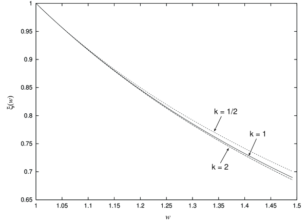
FIG. 2.: Wavefunction sensitivity: The corridor for the Isgur-Wise function as determined using $k=0.5$ and $k=2.0$. The solid line corresponds to $k=1.0$ All curves have the same slope parameter, $\rho^{2}=0.9$.

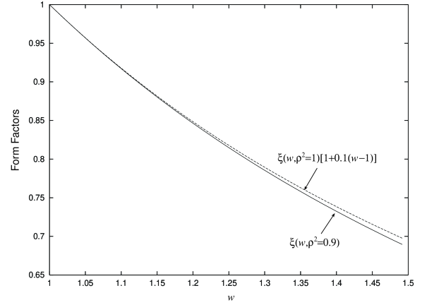
FIG. 3.: Equivalence of a “physical” form factor to an Isgur-Wise function of a shifted slope. The “shifted” IW function $\xi(w,\rho^{2}=0.9)$ and the physical from factor approximation $\xi(w,\rho^{2}=1.0)[1+0.1(w-1)]$ differ only about 2% at $w=1.5$.

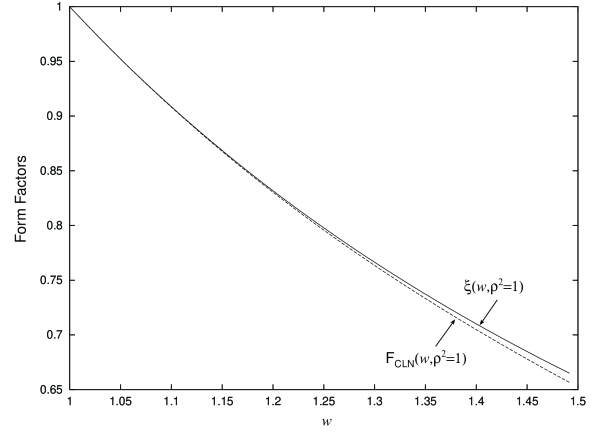
FIG. 4.: The Form Factor $F(w)/F(1)$ from CLN [4] along with an IW function (1) of the same slope parameter, $\rho^{2}=1.0$.

REFERENCES

- [1] N. Isgur and M.B. Wise, Phys. Lett. B232, 113 (1989); B237, 527 (1990).
- [2] G.C. Boyd, B. Grinstein, and R.F. Lebed, Phys. Lett. B353, 306 (1995).
- [3] I. Caprini and M. Neubert, Phys. Lett. B380, 396 (1996).
- [4] I. Caprini, L. Lellouch, and M. Neubert, Nucl. Phys. B530, 151 (1998).
- [5] C.G. Boyd, B. Grinstein, and R.F. Lebed, Phys. Rev. D56, 6895 (1997).
- [6] J.E. Duboscq et al., Phys. Rev. Lett. 76, 3898 (1996)
- [7] J. Bartelt et al, Phys. Rev. Lett. 82, 3746 (1999).
- [8] G. Burdman, Phys. Lett. B284, 133 (1992).
- [9] e.g., S. Veseli and M.G. Olsson, Phys. Rev. D54, 886 (1996).
- [10] A. Falk and M. Neubert, Phys. Rev. D47, 2965 (1993).
- [11] M. Sadzikowski and K. Zalewski, Z. Phys. C59, 677 (1993); H. Høgassen and M. Sadzikowski, Z. Phys. C64, 427 (1994); M.G. Olsson and S. Veseli, Phys. Rev. D51, 2224 (1995); M.R. Ahmady, R.R. Mendel and J.D. Talman, Phys. Rev. D52, 254 (1995).
- [12] S. Veseli and M.G. Olsson, Phys. Lett. B367, 302 (1996).
- [13] A. Duncan, E. Eichten, and H. Thacker, Phys. Lett. B303, 109 (1993); Phys. Rev. D51, 5101 (1995).
- [14] M.G. Olsson and S. Veseli, Phys. Lett. B397, 263 (1997).
- [15] M. Neubert, Phys. Rep. 245, 259 (1994).
- [16] S. Hashimoto et al., Phys. Rev. D61, 014502 (2000)
- [17] M. Luke, Phys. Lett. B252, 447 (1990).
- [18] Z. Ligeti, Y. Nir, and M. Neubert, Phys. Rev. D49, 1302 (1994).
- [19] D. Scora and N. Isgur, Phys. Rev. D52, 2783 (1995).
- [20] A. Abd El-Hady et al., Phys. Rev. D51, 5245 (1995).
- [21] J.N. Simone et al., Nucl.Phys.Proc.Suppl. 73, 399 (1999).