The ($\gamma^{*}\to q\bar{q}$) - Reggeon Vertex in Next-to-Leading Order QCD

Abstract

As a first step towards the computation of the NLO corrections to the photon impact factor in the $\gamma^{*}\gamma^{*}\to\gamma^{*}\gamma^{*}$ scattering process, we calculate the one loop corrections to the coupling of the reggeized gluon to the $\gamma^{*}\to q\bar{q}$ vertex. We list the results for the Feynman diagrams which contribute: all loop integrations are carried out, and the results are presented in the helicity basis of photon, quark, and antiquark.

PACS number(s): 11.55.Jy, 12.38.Bx, 13.60.-r

1 Introduction

The experimental test of the BFKL Pomeron [1] is generally considered to be an important task in strong interaction physics. Recently much interest has been given to the total cross section of the scattering of two highly virtual photons $\sigma_{tot}^{\gamma^{*}\gamma^{*}}$ [2, 3]. This process describes the scattering of two small-size projectiles, and its high energy behavior (at not too large energies) is expected to be described by the BFKL Pomeron. Therefore, a measurement of the reaction $e^{+}e^{-}\to e^{+}e^{-}+X$ by tagging the outgoing leptons at LEP or at a future Linear Collider provides an excellent test of this very important QCD prediction.

So far leading order calculations of the BFKL Pomeron have been compared to LEP data (both OPAL and L3) [4, 5, 6]. In both experiments the data lie above the one gluon exchange curve (commonly called Born approximation), but below the BFKL prediction. Since the next-to-leading order (NLO) corrections to the BFKL kernel have been calculated [7, 8], it is known that the higher corrections will lower the theoretical predictions of the cross section. However, a consistent comparison with the NLO BFKL calculations has not yet been possible: there remains the task of calculating also the next-to-leading order corrections of the coupling of the BFKL Pomeron to the external photons, the so-called photon impact factor.

\begin{picture}(0.0,0.0)\end{picture}

Figure 1: Contributions to the photon impact factor.

The photon impact factor is obtained from the energy discontinuity of the amplitude $\gamma^{*}+\mbox{{reggeon}}\to\gamma^{*}+\mbox{{reggeon}}$ (Fig. 1). In leading order $\alpha_{s}$ this discontinuity is simply the square of the scattering amplitude $\gamma^{*}+\mbox{{reggeon}}\to q\bar{q}$ in the tree approximation, and the reggeon, i.e. the reggeized gluon, can be identified with the elementary t-channel gluon (with a particular helicity). In the next-to-leading order new contributions have to be calculated. For the $q\bar{q}$ intermediate state we need the NLO corrections to the $\gamma^{*}+\mbox{{reggeon}}\to q\bar{q}$ amplitude either on the lhs or on the rhs of the discontinuity line, and the $q\bar{q}g$ intermediate state requires with leading order amplitudes $\gamma^{*}+\mbox{{reggeon}}\to q\bar{q}g$ on both sides of the energy discontinuity line. The task of calculating the NLO corrections to the photon impact factor therefore can therefore be organized in three steps, (i) the calculation of the NLO corrections to the $\gamma^{*}+\mbox{{reggeon}}\to q\bar{q}$ vertex, (ii) the vertex $\gamma^{*}\to q\bar{q}g$ in leading order, and (iii) the integration over the phase space of the intermediate states. In this paper we report on results of the first step, the NLO corrections to the $\gamma^{*}+\mbox{{reggeon}}\to q\bar{q}$ vertex. The vertex is obtained from the high energy limit of the scattering process $\gamma^{*}+q\to q\bar{q}+q$.

2 Technical preliminaries

\begin{picture}(0.0,0.0)\end{picture}

Figure 2: Kinematics of the process $\gamma^{*}+q\to q\bar{q}+q$.

The kinematics is illustrated in Fig. 2. As usual, $q$ and $p$ denote the four momenta of the photon and the incoming quark, resp., and $\varepsilon_{L,t}$ the polarization vectors of the photon. We use $s$ to denote the energy of the $\gamma^{*}q$ scattering process process, and we introduce the invariants $Q^{2}=-q^{2}$, $t_{a}=k^{2}$, $t_{b}=(q-k-r)^{2}$, $M^{2}=(q+r)^{2}$, $t=r^{2}$, and $x=Q^{2}/2p\cdot{q}$ for the Bjorken scaling variable. For simplicity, in the calculation of this paper we treat the quarks as massless. The momenta $k$ and $r$ can be written in the Sudakov decomposition form, i.e.,

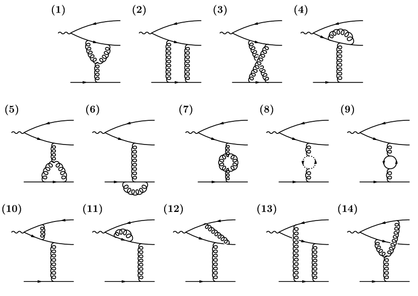
Figure 3: Feynman diagrams for the process $\gamma^{*}+q\to q\bar{q}+q$.

$$k=\alpha q^{\prime}+\beta p+k_{\perp}\;,$$ (1)

$$r=\frac{t}{s}q^{\prime}-\frac{t_{a}+t_{b}}{s}p+r_{\perp}\;,$$ (2)

where $q^{\prime}=q+xp$ and

$$\beta s=\frac{k_{\perp}^{2}}{1-\alpha}-Q^{2}.$$ (3)

The Feynman diagrams which contribute to our NLO-calculation are listed in Fig. 3. In addition to the graphs shown (all diagrams, except for Fig. 3.14), we have to add those diagrams where the t-channel gluon couples to the outgoing antiquark rather than the outgoing quark. It is easy to see that, for the color octet $t$-channel configuration, the sum of all diagrams has to be antisymmetric if we interchange quark and antiquark: $k\to q-k-r$, $\lambda\to\lambda^{\prime}$. In particular, the ’box’ graph shown in Fig. 3.14 has to be antisymmetric by itself. We will use the Feynman gauge throughout the calculation, and for the t-channel gluons we decompose the metric tensor according to

$$g_{\mu\nu}=\frac{2}{s}(p_{\mu}q_{\nu}^{\prime}+p_{\nu}q_{\mu}^{\prime})+g_{\mu\nu}^{\perp}.$$ (4)

In our calculation we retain only the first term, since the remaining ones are suppressed by powers of the energy. We use the helicity formalism, and our results will be expressed in terms of the following matrix elements:

$$H_{T}^{a} = \bar{u}(k+r,\lambda)\not\!{p}\not\!{k}\not\!{\varepsilon}\;\lambda^{a}v(q-k,\lambda^{\prime})\;,$$ (5)

$$\bar{H}_{T}^{a} = \bar{u}(k+r,\lambda)\not\!{\varepsilon}\;(\not\!{q}-\not\!{k}-\not\!{r})\;\not\!{p}\;\lambda^{a}v(q-k,\lambda^{\prime})\;,$$ (6)

$$H_{\varepsilon}^{a} = \bar{u}(k+r,\lambda)\not\!{\varepsilon}\;\lambda^{a}v(q-k,\lambda^{\prime})\;,$$ (7)

$$H_{k}^{a} = \bar{u}(k+r,\lambda)\not\!{k}\;\lambda^{a}v(q-k,\lambda^{\prime})\;,$$ (8)

$$H_{p}^{a} = \bar{u}(k+r,\lambda)\not\!{p}\;\lambda^{a}v(q-k,\lambda^{\prime})\;,$$ (9)

where $\lambda^{a}(a=1,\cdots,8)$ are the color matrices, and $\lambda$ and $\lambda^{\prime}$ denote the helicities of the outgoing quark pair. When interchanging quark and antiquark lines it will be convenient to use the following identity

$$H_{T}^{a}+\bar{H}_{T}^{a}=sH_{\varepsilon}^{a}-2\varepsilon\cdot pH_{k}^{a}-2\varepsilon\cdot rH_{p}^{a}\;.$$ (10)

We organize our calculations in the following order. We first consider those diagrams (Fig. 3.1–9) which can be viewed as “elastic scattering of two quarks”, with the upper ‘incoming’ quark carrying the mass $t_{a}$. Correspondingly, the diagrams not shown in Fig. 3 define quark-quark scattering with the upper ‘incoming’ antiquark having the mass $t_{b}$. Together with the correction at the photon vertex (Fig. 3.10) and the quark self-energy (Fig. 3.11), these diagrams are the ones which have to be made ultraviolet finite by renormalization. In the final part we turn to the calculation of the box diagrams in Figs. 3.12 and 3.14, and the pentagon graph shown in Fig. 3.13.

We are interested in the high energy limit, where

$$t,\;Q^{2},\;t_{a},\;t_{b},\;M^{2}\;\ll s\;,$$ (11)

and we do not impose any restriction on the remaining invariants. The Regge ansatz for the scattering amplitude $\gamma^{*}q\to(q\bar{q})q$ takes the form:

$$T=\Gamma_{\gamma^{*}\to q\bar{q}}^{a}\frac{s}{t}\left[\left(\frac{\quad s}{-t}\right)^{\omega}+\left(\frac{-s}{-t}\right)^{\omega}\right]\Gamma_{qq}^{a}\;.$$ (12)

Here, $1+\omega$ is the gluon trajectory. Expanding all terms in powers on the strong coupling $g$, we have

$$\omega = g^{2}\;\omega^{(1)}+g^{4}\;\omega^{(2)}\;,$$ (13)

$$\Gamma_{\gamma^{*}\to q\bar{q}}^{a} = g\;\Gamma_{\gamma^{*}\to q\bar{q}}^{(0),a}+g^{3}\;\Gamma_{\gamma^{*}\to q\bar{q}}^{(1),a}\;,$$ (14)

$$\Gamma_{qq}^{a} = g\;\Gamma_{qq}^{(0),a}+g^{3}\;\Gamma_{qq}^{(1),a}\;.$$ (15)

After substituting corresponding elements in Eq.(12) with above expansions, one obtains the following structure of the amplitude

$$T=g^{2}\;T^{(0)}+g^{4}\;T^{(1)}$$ (16)

with

$$T^{(0)}=\Gamma_{\gamma^{*}\to q\bar{q}}^{(0),a}\;\frac{2s}{t}\;\Gamma_{qq}^{(0),a}$$ (17)

and

$$T^{(1)} = \Gamma_{\gamma^{*}\to q\bar{q}}^{(1),a}\;\frac{2s}{t}\;\Gamma_{qq}^{(0),a}+\Gamma_{\gamma^{*}\to q\bar{q}}^{(0),a}\;\frac{2s}{t}\Gamma_{qq}^{(1),a}$$ (18)

$$+\,\Gamma_{\gamma^{*}\to q\bar{q}}^{(0),a}\;\frac{s}{t}\,\omega^{(1)}\left[\ln\frac{{\quad s}}{-t}+\ln\frac{-s}{-t}\right]\Gamma_{qq}^{(0),a}.$$

Here, the $e_{f}$ represents the charge value of the interacting quark, and the lowest-order expressions on the rhs of (18) are

$$\Gamma_{qq}^{(0),a} = \frac{1}{s}\bar{u}(p-r,\,\lambda_{q^{\prime}})\not\!{q}^{\prime}\lambda^{a}u(p,\,\lambda_{q})\,,$$ (19)

$$\omega^{(1)}(t) = \frac{2N_{c}}{(4\pi)^{2-\epsilon}}\,\frac{c_{\Gamma}}{\epsilon}\,(-t)^{-\epsilon}\,,$$ (20)

$$\Gamma_{\gamma^{*}\to q\bar{q}}^{(0),a} = -ie_{f}e\left(\frac{H_{T}^{a}}{st_{a}}-\frac{\bar{H}_{T}^{a}}{st_{b}}\right)\,,$$ (21)

with $D=4-2\;\epsilon$ and

$$c_{\Gamma}=\frac{\Gamma(1+\epsilon)\Gamma^{2}(1-\epsilon)}{\Gamma(1-2\epsilon)}\approx 1-\gamma_{E}\epsilon+\frac{1}{2}\left(\gamma_{E}^{2}-\frac{\pi^{2}}{6}\right)\epsilon^{2}+{\cal O}(\epsilon^{3})\,$$ (22)

Here $\lambda_{q}$ and $\lambda_{q^{\prime}}$ are the helicities of the incoming and outgoing quark, resp., and $\lambda^{a}$ are the generators of the colour group. In this paper we will present the results of Figs. 3.1 – 3.14 which can be cast into the form of the rhs of (18). All pieces except for $\Gamma_{\gamma^{*}\to q\bar{q}}^{(1),a}$ are known from earlier calculations. In particular, the Born result for $\Gamma_{\gamma^{*}\to q\bar{q}}^{(0),a}$ is well known in the context of the photon wave function formalism, and it is available for definite helicity states [9]. The higher order corrections to the quark-quark-reggeon vertex, $g^{3}\Gamma_{qq}^{(1)}(t)$, have been calculated in [10]. For vanishing quark masses these corrections are (following the notations of [10]):

$$\Gamma_{qq}^{(1),a}(t)=\lambda^{a}\left(\Gamma_{qq}^{(1)}(q\bar{q}-\mbox{state})+\Gamma_{qq}^{(1)}(gg-\mbox{state})\right)\delta_{\lambda_{q}\lambda_{q^{\prime}}},$$ (23)

with

$$\Gamma_{qq}^{(1)}(q\bar{q}-\mbox{state}) =\frac{(-t)^{-\epsilon}}{(4\pi)^{2-\epsilon}}\left[-\frac{n_{f}}{2}\,\frac{c_{\Gamma}}{\epsilon(1-2\epsilon)}\left(1-\frac{1}{3-2\epsilon}\right)+\frac{c_{\Gamma}}{2N_{c}}\left(\frac{2}{\epsilon^{2}}+\frac{3}{\epsilon}+8\right)\right]$$ (24)

$$\Gamma_{qq}^{(1)}(gg-\mbox{state}) =\frac{N_{c}\,(-t)^{-\epsilon}}{(4\pi)^{2-\epsilon}}\left[-\frac{c_{\Gamma}}{\epsilon^{2}}+\frac{1}{3}\frac{c_{\Gamma}}{\epsilon}+\frac{13}{18}+\frac{\pi^{2}}{2}\right].$$ (25)

Inserting these results on the rhs of (18) we can easily obtain $\Gamma_{\gamma^{*}\to q\bar{q}}^{(1),a}$, which is the goal of this paper.

For future purposes it will be important to note that the vertex $\Gamma_{\gamma^{*}\to q\bar{q}}^{(1),a}$ in (12) is expected [11] to have a rather complex structure. For example, in the limit of large diffractive masses it will be more convenient to write (12) as a sum of two different expressions: the first one depending on $M^{2}$ and $s$, the second one on $\alpha s$ and $s$ (or $(1-\alpha)s$). This decomposition exhibits the reggeization of both the gluon and the quark. A detailed discussion of the large-$M^{2}$ limit will be presented in a seperate paper [12].

3 Analytic Results

We write the NLO amplitude $T^{(1)}$ for the process $\gamma^{*}+q\to q\bar{q}+q$ as a sum of the different Feynman diagrams:

$$T^{(1)}=\sum_{i=1}^{13}\big{(}A_{i}+\bar{A_{i}})+A_{14}.$$ (26)

The subscripts $i$ refer to the numbering in Fig. 3, and the amplitudes $\bar{A_{i}}$ correspond to the diagrams which are not shown in Fig. 3: they are obtained by interchanging the couplings of $t$-channel gluons between quark and antiquark lines. Formally, we substitute

$$k\leftrightarrow q-k-r,\;\alpha\leftrightarrow(1-\alpha),\;t_{a}\leftrightarrow t_{b},$$

$$H^{a}_{T}\leftrightarrow\bar{H}^{a}_{T},\;\varepsilon\cdot k\leftrightarrow-\varepsilon\cdot(k+r),\;\lambda\leftrightarrow\lambda^{\prime},$$ (27)

Under these replacements the matrix elements (7)–(9) remain unchanged. In addition, for all diagrams except for Fig. 3.14 we have to include an overall minus sign when interchanging quark and antiquark. $A_{14}$ is already antisymmetric by itself with respect to the interchange of quark and antiquark.

3.1 Calculational methods

Before presenting explicit analytic expressions for all diagrams we briefly outline the methods we have used to obtain the results.

Starting from the standard Feynman rules of QCD we project the color in the $t$-channel into the antisymmetric octet and proceed by introducing Feynman parameters $x_{i}$ to combine the denominators for the integration of the loop momentum. Only for the simplest diagrams these steps are easily performed by hand. Particularly for the diagrams Fig. 3.12–14 this step becomes too tedious. Therefore, we have used the computer algebra system Mathematica with the package FeynCalc [15], in order to reduce the numerators to expressions which contain the helicity matrix elements (5) to (9), monomials $x_{i}x_{j}\cdots$ in the Feynman parameters and, of course, the kinematical invariants. Those diagrams, where the loop integral itself does not depend on the large scale $s$, the box diagrams Fig. 3.12 and Fig. 3.14, have to be calculated exactly. The only high energy approximation results from the gluon nonsense helicity (i.e. the first term in (4). Diagram Fig. 3.13, on the other hand, has first been calculated exactly, and then the high energy limit (11) has been taken.

To consider the loop integrations, we had to deal with integrals over the loop momentum itself, which could be easily performed by the usual shift, and with the remaining integrals of the Feynman parameters. Integrals of the latter type are either known, or they could be obtained from known ones with the help of recurrence relations to ${\cal O}(\epsilon^{0})$ in dimensional regularization. The technical background for these methods is given in [13] and has been applied to almost all cases we are interested in by [14]. We have written a Mathematica package to easily call the results of [14]. In most cases the integrals are recursively expressed in terms of special functions, representing a particular combination of logarithms and dilogarithms for a given $n$-point function. In the case of diagram Fig. 3.14 we have calculated explicit results for integrals with two and three Feynman parameters in the numerator using the derivative method [13]. Also for this task we have used Mathematica.

Finally, after carrying out the integrals, i.e. replacing the monomials of Feynman parameters in our amplitudes with the explicit expressions from our Mathematica package, we have used again FeynCalc to take the high energy limit in the diagrams Figs. 3.2, 3, and 13, and to carry out some simplifying algebra. A few final simplifications had to be done by hand. The expressions that we have obtained in this way will be listed in the remainder of this section.

3.2 Quark-quark Scattering

It is suggestive to view the diagrams Figs. 3.1–9 as a quark-quark scattering processes with one of the incoming quarks being off-shell (with virtuality $t_{a}$). We focus on those diagrams in Fig. 3, where the $t$-channel gluon(s) couples to the quark. Those diagrams where the gluon(s) couples to the antiquark are easily obtained by performing the substitutions described after (26).

Diagram Fig. 3.1 is one of many three point functions with two massive external legs. Loop integrals of this type are well-known, and we have calculated them both by hand and by using computer algebra as outlined above.

$$A_{1}\, =\,\frac{N_{c}}{2}\frac{1}{(4\pi)^{2-\epsilon}}\bigg{\{}A^{(0)}\bigg{[}\frac{2c_{\Gamma}}{\epsilon^{2}}\frac{t_{a}}{t-t_{a}}\left((-t_{a})^{-\epsilon}-(-t)^{-\epsilon}\right)$$ (28)

$$+\frac{c_{\Gamma}}{\epsilon}(-t)^{-\epsilon}+2+\frac{2t}{t-t_{a}}{\rm{ln}}\frac{t}{t_{a}}\bigg{]}-\frac{(-iee_{f})\alpha}{t-t_{a}}H^{a}_{\varepsilon}\frac{2s}{t}\Gamma_{qq}^{(0),a}$$

$$\times\bigg{[}-\frac{c_{\Gamma}}{\epsilon^{2}}\frac{t_{a}}{t-t_{a}}\left((-t_{a})^{-\epsilon}-(-t)^{-\epsilon}\right)+\frac{c_{\Gamma}}{\epsilon}(-t)^{-\epsilon}+1-\frac{t}{t-t_{a}}{\rm{ln}}\frac{t}{t_{a}}\bigg{]}\bigg{\}}\;.$$

Here and in the following, we use

$$A^{(0)}=-iee_{f}\frac{H_{T}^{a}}{st_{a}}\,\frac{2s}{t}\,\Gamma_{qq}^{(0),a}$$ (29)

as a shorthand notation.

In the diagrams Fig. 3.2 and Fig. 3.3 we have to deal with four-point integrals, where one of the external legs is off-mass shell. Here we make use of the shorthand notations listed in the appendix. The result for the sum of the two diagrams is:

$$A_{2+3}= -A^{(0)}N_{c}\frac{1}{(4\pi)^{2-\epsilon}}\left\{\frac{c_{\Gamma}}{\epsilon^{2}}\Big{[}(\alpha s)^{-\epsilon}+(-\alpha s)^{-\epsilon}+(-t)^{-\epsilon}-2(-t_{a})^{-\epsilon}\right.$$

$$-\left.\frac{t}{t-t_{a}}\left((-t)^{-\epsilon}-(-t_{a})^{-\epsilon}\right)\Big{]}+{\rm{Ld}_{0}^{1m}}(\alpha s,t,t_{a})+{{\rm{Ld}}_{0}^{1m}}(-\alpha s,t,t_{a})\right\}$$ (30)

with

$${\rm{Ld}}_{0}^{1m}(\alpha s,t,t_{a})={\rm{Li}}_{2}(1-\frac{t}{t_{a}})+{\rm{Li}}_{2}(1-\frac{\alpha s}{t_{a}})+{\rm{ln}}\frac{t}{t_{a}}{\rm{ln}}\frac{\alpha s}{t_{a}}-\frac{\pi^{2}}{6}\;.$$

Here, $\rm{Li}_{2}$ is the standard dilogarithm function defined as

$${\rm{Li}}_{2}(x)=-\int^{1}_{0}\frac{\ln(1-xt)}{t}dt\;.$$ (31)

In order to exhibit the energy dependence we rewrite this expression:

$$A_{2+3}= -A^{(0)}\frac{N_{c}}{(4\pi)^{2-\epsilon}}\Big{\{}-\frac{c_{\Gamma}(-t)^{-\epsilon}}{\epsilon}\left[\ln\frac{{\alpha s}}{-t}+\ln\frac{-\alpha s}{-t}\right]$$

$$+2\,{\rm Li}_{2}\left(1-\frac{t}{t_{a}}\right)+\left(\ln\frac{t}{t_{a}}\right)^{2}+\frac{\pi^{2}}{3}+(-t)^{-\epsilon}\left[\frac{2c_{\Gamma}}{\epsilon^{2}}-\pi^{2}\right]$$

$$+\frac{c_{\Gamma}}{\epsilon^{2}}\Big{[}(-t)^{-\epsilon}-2(-t_{a})^{-\epsilon}-\frac{t}{t-t_{a}}\left((-t)^{-\epsilon}-(-t_{a})^{-\epsilon}\right)\Big{]}\Big{\}}.$$ (32)

From these two diagrams (and from their respective partners $\bar{A}_{2+3}$) we already get the complete $\ln s$ dependence of our result, in agreement with the rhs of (18). In detail, the first line of (3.2) contains, apart from the $\ln\alpha$ dependence, the leading order trajectory function $\omega^{(1)}(t)$ (cf.(20)). Furthermore, if we take the limit $t_{a}\to 0$ in the last two lines, we are left with only the last term of the second line. One half of this term will go to the lower vertex (25) (the same result could also have been deduced from  [10]). Therefore, the contribution from diagrams 2 and 3 to $\Gamma_{\gamma^{*}\to q\bar{q}}^{(1),a}$ is just

$$iee_{f}\frac{H_{T}^{a}}{st_{a}}\frac{N_{c}}{(4\pi)^{2-\epsilon}}\Big{\{}-\frac{2c_{\Gamma}(-t)^{-\epsilon}}{\epsilon}\ln\alpha+2\,{\rm Li}_{2}\left(1-\frac{t}{t_{a}}\right)+\left(\ln\frac{t}{t_{a}}\right)^{2}+\frac{\pi^{2}}{3}$$

$$+\frac{(-t)^{-\epsilon}}{2}\left[\frac{2c_{\Gamma}}{\epsilon^{2}}-\pi^{2}\right]+\frac{c_{\Gamma}}{\epsilon^{2}}\Big{[}(-t)^{-\epsilon}-2(-t_{a})^{-\epsilon}-\frac{t}{t-t_{a}}\left((-t)^{-\epsilon}-(-t_{a})^{-\epsilon}\right)\Big{]}\Big{\}}.$$ (33)

We emphasize, once more, that the two diagrams $A_{2+3}+\bar{A}_{2+3}$ provide the complete $\ln s$ dependence on the rhs of (12). At first sight one might expect that also the pentagon diagrams $A_{13}+\bar{A}_{13}$ might contribute to the energy dependence. Later we will show that, in fact, this is not the case.

The calculation of Fig. 3.4 is very similar to the calculation of Fig. 3.1. We find:

$$A_{4}=-\frac{1}{2N_{c}}\frac{1}{(4\pi)^{2-\epsilon}}\bigg{\{}A^{(0)}\bigg{[}\frac{2c_{\Gamma}}{\epsilon^{2}}\frac{t}{t-t_{a}}\left((-t_{a})^{-\epsilon}-(-t)^{-\epsilon}\right)-\frac{c_{\Gamma}}{\epsilon}(-t)^{-\epsilon}$$ (34)

$$\;-4+\frac{2t+t_{a}}{t-t_{a}}{\rm{ln}}\frac{t}{t_{a}}\bigg{]}-iee_{f}\,\alpha H^{a}_{\varepsilon}\frac{2s}{t}\Gamma_{qq}^{(0),a}\Big{[}\frac{2c_{\Gamma}}{\epsilon^{2}}\frac{t\left((-t_{a})^{-\epsilon}-(-t)^{-\epsilon}\right)}{(t-t_{a})^{2}}$$

$$\;-\frac{2c_{\Gamma}}{\epsilon}\frac{(-t)^{-\epsilon}}{t-t_{a}}+\frac{3t+2t_{a}}{(t-t_{a})^{2}}{\rm{ln}}\frac{t}{t_{a}}-\frac{5}{t-t_{a}}\Big{]}\bigg{\}}\;.$$

Diagrams Fig. 3.5 and Fig. 3.6 are needed to obtain the NLO corrections to the lower vertex $\Gamma^{(1),a}_{qq}$. In agreement with  [10] we find:

$$A_{5}=-A^{(0)}\;\frac{N_{c}c_{\Gamma}}{(4\pi)^{2-\epsilon}}\left(\frac{(-t)^{-\epsilon}}{2\epsilon}+1\right)\;,$$ (35)

and

$$A_{6}=A^{(0)}\;\frac{1}{(4\pi)^{2-\epsilon}}\frac{c_{\Gamma}}{2N_{c}}(-t)^{-\epsilon}\left(\frac{2}{\epsilon^{2}}+\frac{3}{\epsilon}+{8}\right)\;.$$ (36)

We note that they can be obtained from Eqs. (28) and (34) by choosing $\epsilon<0$ and taking the limit $t_{a}\to 0$.

The calculation of diagrams Figs. 3.7–9 is straightforward. They contribute to both the upper and the lower vertex:

$$A_{7+8}=A^{(0)}\;\frac{N_{c}c_{\Gamma}}{(4\pi)^{2-\epsilon}}\frac{(-t)^{-\epsilon}}{2\epsilon(1-2\epsilon)}\left(\frac{1}{3-2\epsilon}+3\right)\;,$$ (37)

Similarly, the $q\bar{q}$-contribution to the gluon-self-energy in Fig. 3.9 leads to

$$A_{9}=A^{(0)}n_{f}\;\frac{c_{\Gamma}}{(4\pi)^{2-\epsilon}}\frac{(-t)^{-\epsilon}}{\epsilon(1-2\epsilon)}\left(\frac{1}{3-2\epsilon}-1\right).$$ (38)

These diagrams contribute with equal weight to both the upper and to the lower vertex. Therefore, in order to complete the upper reggeon-quark-quark vertex with one off-shell quark, we simply add $1/2$ of the sum of (37) and (38) to the contributions (28), (34), and (35). Similarly, the lower reggeon-quark-quark vertex with all quarks being on-shell is obtained by adding $1/2$ of the sum of (37) and (38) to (35), (36) and the contribution of the box diagrams Figs. 3.2 and 3.3:

$$-A^{(0)}\frac{N_{c}}{(4\pi)^{2-\epsilon}}\frac{(-t)^{-\epsilon}}{2}\left[\frac{2c_{\Gamma}}{\epsilon^{2}}-\pi^{2}\right].$$ (39)

To summarize, so far we have analyzed the diagrams Figs. 3.1–9. From Figs. 3.5, 3.6, $1/2$ of Figs. 3.7–9, and from a piece of Fig. 3.2 and 3.3. we have reproduced the lower reggeon-quark-quark vertex of  [10]. From Figs. 3.1, 3.4, $1/2$ of Figs. 3.7–9, and from the major part of Figs. 3.2 and 3.3 we have computed a new reggeon-quark-quark vertex with one quark having the mass $t_{a}$. Moreover, from Figs. 3.2 and 3.3. we have extracted the $\ln s$ terms of the rhs of (18). The remaining diagrams Figs. 3.10–14 provide contributions to the upper vertex $\Gamma^{(1),a}_{\gamma^{*}\to qq}$ only.

3.3 Vertex correction and quark self-energy

In this subsection we present the results of the vertex correction Fig. 3.10:

$$A_{10} =-\frac{C_{\rm{F}}}{(4\pi)^{2-\epsilon}}\bigg{\{}A^{(0)}\bigg{[}\frac{2c_{\Gamma}}{\epsilon^{2}}\frac{Q^{2}}{Q^{2}+t_{a}}\left((Q^{2})^{-\epsilon}-(-t_{a})^{-\epsilon}\right)+\frac{c_{\Gamma}}{\epsilon}(-t_{a})^{-\epsilon}$$ (40)

$$+4+\frac{3Q^{2}}{Q^{2}+t_{a}}{\rm{ln}}\frac{-t_{a}}{Q^{2}}\bigg{]}-\Gamma^{\prime}\frac{2s}{t}\Gamma_{qq}^{(0),a}\bigg{[}\frac{4c_{\Gamma}}{\epsilon^{2}}\frac{Q^{2}}{Q^{2}+t_{a}}\left((Q^{2})^{-\epsilon}-(-t_{a})^{-\epsilon}\right)$$

$$+\frac{4c_{\Gamma}}{\epsilon}(-t_{a})^{-\epsilon}+10\left(1+\frac{Q^{2}}{Q^{2}+t_{a}}\right){\rm{ln}}\frac{-t_{a}}{Q^{2}}\bigg{]}\bigg{\}}$$

with

$$\Gamma^{\prime}=-iee_{f}\,\frac{H_{p}^{a}}{s}\frac{\varepsilon\cdot k}{Q^{2}+t_{a}},$$ (41)

and for the quark self-energy Fig. 3.11:

$$A_{11}=-A^{(0)}\frac{C_{\rm{F}}}{(4\pi)^{2-\epsilon}}(-t_{a})^{-\epsilon}\frac{c_{\Gamma}(1-\epsilon)}{\epsilon(1-2\epsilon)}\;.$$ (42)

Eqs. (40) and (42) provide new contributions to the vertex $\Gamma^{(1),a}_{\gamma^{*}\to qq}$.

3.4 The Box diagram Fig. 3.12

In this subsection we give the result of the diagram Fig. 3.12, which was calculated entirely with the help of the computer algebra (in [14] this diagram has been named ‘adjacent box’). The result will be expressed as follows:

$$A_{12}=\Gamma^{(0),a}_{qq}\frac{2\,s}{t}\left(\frac{-iee_{f}}{s}\right)\left(-\frac{1}{2N_{c}}\right)\frac{c_{\Gamma}}{(4\pi)^{2-\epsilon}}\left[\frac{1}{\epsilon^{2}}A_{12}^{(-2)}+\frac{1}{\epsilon}A_{12}^{(-1)}+A_{12}^{(0)}\right].$$ (43)

Starting with the divergent terms, we have

$$A_{12}^{(-2)} =\frac{2\alpha\,H^{a}_{\varepsilon}\,s\,t\,({(-t)}^{-\epsilon}-{(-t_{a})}^{-\epsilon})}{(t-t_{a})^{2}}+2H^{a}_{T}\bigg{[}\frac{{(-t)}^{-\epsilon}-{(-t_{a})}^{-\epsilon}}{t-t_{a}}\;$$ (44)

$$+\;\frac{{(-t_{a})}^{-\epsilon}-{(Q^{2})}^{-\epsilon}}{Q^{2}+t_{a}}+\frac{-{(-M^{2})}^{-\epsilon}+{(Q^{2})}^{-\epsilon}+{(-t)}^{-\epsilon}-2{(-t_{a})}^{-\epsilon}}{t_{a}}\bigg{]}$$

$$-\frac{4Q^{2}\varepsilon\cdot kH_{p}^{a}}{(Q^{2}+t_{a})^{2}}\left((Q^{2})^{-\epsilon}-(-t_{a})^{-\epsilon}\right)$$

and

$$A_{12}^{(-1)}= 4\,\epsilon\cdot k\,H^{a}_{p}\left[\frac{({(-t)}^{-\epsilon}-{(-t_{a})}^{-\epsilon})}{M^{2}}-\frac{{(-t_{a})}^{-\epsilon}}{Q^{2}+t_{a}}\right]$$

$$+H^{a}_{\varepsilon}s\,\left[\frac{2\,\alpha(-t)^{-\epsilon}}{t-t_{a}}+\frac{(1-\alpha)\,({(-t)}^{-\epsilon}-{(-t_{a})}^{-\epsilon})}{M^{2}}\right].$$ (45)

The ${\cal O}(\epsilon^{0})$ term for the this adjacent box is expressed in terms of many different functions, related to this loop integral. For convenience, the definitions of these functions are listed in the appendix.

$$A_{12}^{(0)} =-2(2H^{a}_{T}+s\alpha H^{a}_{\varepsilon}){\rm Lc}_{0}(-Q^{2},M^{2},t)$$

$$+\big{\{}3H^{a}_{T}M^{2}+H^{a}_{k}[6\varepsilon\cdot pM^{2}+2s((8\alpha-3)\varepsilon\cdot k+(5\alpha-3)\varepsilon\cdot r)]$$

$$\quad-s\alpha\,H^{a}_{\varepsilon}(3t_{a}-2t_{b}-Q^{2})-2H^{a}_{p}(2Q^{2}\varepsilon\cdot r+\varepsilon\cdot k(M^{2}-Q^{2}-3t_{b}))\big{\}}\frac{{\rm Lc}_{1}(M^{2},-Q^{2},t)}{M^{2}}$$

$$+2\big{\{}H^{a}_{T}M^{2}+2H^{a}_{k}(M^{2}\varepsilon\cdot p-s[\varepsilon\cdot k+(1-\alpha)\varepsilon\cdot r])+2sH^{a}_{\varepsilon}[(1-\alpha)t+\alpha Q^{2}+t_{a}]$$

$$\quad-4H^{a}_{p}[\varepsilon\cdot k(2M^{2}+Q^{2}+t)+\varepsilon\cdot r(Q^{2}+t_{a})]\big{\}}\frac{{\rm Lc}_{1}(-Q^{2},M^{2},t)}{M^{2}}$$

$$+\big{\{}2\varepsilon\cdot kH^{a}_{p}(2M^{2}-2Q^{2}-t_{a})-(1-\alpha)sQ^{2}H^{a}_{\varepsilon}-H^{a}_{T}(Q^{2}+t_{a})$$

$$\quad-2H^{a}_{k}[\varepsilon\cdot k(1-2\alpha)s+\varepsilon\cdot p(Q^{2}+t_{a})]\big{\}}\frac{{\rm Lc}_{1}^{2m}(-Q^{2},t_{a})}{M^{2}}$$

$$-2\big{\{}2s\alpha(3\varepsilon\cdot k+\varepsilon\cdot r)H^{a}_{k}+sH^{a}_{\varepsilon}[\alpha(M^{2}-Q^{2}-3t_{a})+(t-t_{a})]$$

$$\quad+H^{a}_{p}[3\varepsilon\cdot rt_{a}+\varepsilon\cdot k\,(4\,t-t_{a})]\big{\}}\frac{{\rm Lc}_{1}^{2m}(t_{a},t)}{M^{2}}$$

$$+2\big{\{}4\varepsilon\cdot pM^{2}\,H^{a}_{k}+3M^{2}H^{a}_{T}-s[\alpha(M^{2}-2\,Q^{2}-t)+t]H^{a}_{\varepsilon}$$

$$\quad-2[\varepsilon\cdot r\,Q^{2}+\varepsilon\cdot k\,(M^{2}+Q^{2}+2\,t)]H^{a}_{p}\big{\}}\frac{{\rm Lc}_{1S}(-Q^{2},M^{2},t)}{M^{2}t_{a}}$$

$$+4\alpha sH^{a}_{\varepsilon}{\rm Lc}_{2}^{2m}(t_{a},t)-8\,\varepsilon\cdot k\,H^{a}_{p}{\rm Lc}_{2}^{2m}(-Q^{2},t_{a})$$

$$-2\,\big{\{}H^{a}_{T}\,M^{2}+2H^{a}_{k}[\varepsilon\cdot pM^{2}-s((1-2\alpha)\varepsilon\cdot k+(1-\alpha)\varepsilon\cdot r)]$$

$$\quad+2\,H_{p}^{a}\varepsilon\cdot k(2M^{2}+t-t_{a})-\alpha sH^{a}_{\varepsilon}(Q^{2}+t_{a})\big{\}}\frac{{\rm Lc}_{2}(-Q^{2},M^{2},t)}{M^{2}}$$

$$+2\big{\{}2\varepsilon\cdot k(t_{a}-M^{2})H^{a}_{p}+(Q^{2}+t_{a})H^{a}_{T}$$

$$\quad+2[(1-2\,\alpha)s\varepsilon\cdot k+\varepsilon\cdot p(Q^{2}+t_{a})]H^{a}_{k}\big{\}}\frac{{\rm Lc}_{3}(M^{2},-Q^{2},t)}{M^{2}}$$

$$-2(2\varepsilon\cdot k\,H^{a}_{p}+s\alpha\,H^{a}_{\varepsilon}){\rm Lc}_{3}(-Q^{2},M^{2},t)-4\,H^{a}_{T}\frac{{\rm Ld}_{0}^{a}(t_{a},M^{2},-Q^{2},t)}{t_{a}}$$

$$+2\big{\{}t_{b}M^{2}H^{a}_{T}+st_{a}[\alpha\,(Q^{2}+t)-Q^{2}-2\,\alpha\,M^{2}-t_{b}]H^{a}_{\varepsilon}$$

$$\quad-2t_{a}[\varepsilon\cdot k\,(2M^{2}+Q^{2}+t)+\varepsilon\cdot r\,(t-t_{b})]H^{a}_{p}-2[(-(\varepsilon\cdot p\,M^{2})+(\varepsilon\cdot k+\varepsilon\cdot r)s)t_{a}$$

$$\quad+s\alpha(2\,\varepsilon\cdot k\,M^{2}-\varepsilon\cdot r\,t_{a})]H^{a}_{k}\big{\}}\frac{{\rm Ld}_{1}(t_{a},M^{2},-Q^{2},t)}{M^{2}t_{a}}$$

$$-2\{H^{a}_{T}+s\,H^{a}_{\varepsilon}-2\,\varepsilon\cdot r\,H^{a}_{p}\}{\rm Ld}_{1S}(t_{a},M^{2},-Q^{2},t)$$

$$+\big{\{}4[\alpha\,s\,(6\,\varepsilon\cdot k\,(t-t_{b})+2\,\varepsilon\cdot k\,t_{a}+2\,\varepsilon\cdot r\,Q^{2}+3\,\varepsilon\cdot r\,t_{a})$$

$$\quad-t_{a}(\varepsilon\cdot p\,M^{2}+s\,(\varepsilon\cdot k+\varepsilon\cdot r))]H^{a}_{k}+4[2\,\varepsilon\cdot r\,t_{a}\,(t-t_{b})+\varepsilon\cdot k\,(2t(Q^{2}+t)$$

$$\quad+(t-t_{a})(t_{a}-2t_{b}))]H^{a}_{p}-2\,s[\alpha(Q^{2}+t_{a})(2\,Q^{2}+5t_{a})-2(Q^{2}t+t_{a}t_{b})]\,H_{\varepsilon}^{a}$$

$$\quad-2H^{a}_{T}M^{2}t_{a}\big{\}}\frac{{\rm Ld}_{21}(t_{a},M^{2},-Q^{2},t)}{2t_{a}M^{2}}$$

$$+2\big{\{}-(Q^{2}+t_{a})M^{2}H^{a}_{T}+2[\varepsilon\cdot r\,(Q^{2}+t_{a})\,(t-t_{b})$$

$$\quad+\varepsilon\cdot k\,((Q^{2}+t_{a})(t-t_{a})+(t-t_{b})^{2})]H^{a}_{p}-2[\varepsilon\cdot p\,M^{2}\,(Q^{2}+t_{a})$$

$$\quad-s\,((1-\alpha)\,\varepsilon\cdot r\,(Q^{2}+t_{a})-\varepsilon\cdot k\,(Q^{2}+t_{a}-(1-3\,\alpha)\,M^{2}))]H^{a}_{k}$$

$$\quad+s\,[(1-\alpha)(Q^{2}t+t_{a}t_{b})-\alpha\,(Q^{2}+t_{a})^{2}]H^{a}_{\varepsilon}\big{\}}\frac{{\rm Ld}_{22}(t_{a},M^{2},-Q^{2},t)}{M^{2}\,t_{a}}$$

$$+\frac{2\,s\,\alpha\,(Q^{2}+2\,t_{a})\,H^{a}_{\varepsilon}\,{\rm Ld}_{24}(t_{a},M^{2},-Q^{2},t)}{t_{a}}$$

$$+\big{\{}24\,\varepsilon\cdot pM^{2}\,H^{a}_{k}+18\,M^{2}H^{a}_{T}-6\,s[t-t_{a}-\alpha\,(3\,Q^{2}+2t_{a}+t_{b})]H^{a}_{\varepsilon}$$

$$\quad-12[\varepsilon\cdot k\,(3\,t-2t_{a}-t_{b})+\varepsilon\cdot r\,(Q^{2}+t_{a})\ )]H^{a}_{p}\big{\}}\frac{{\rm Ld}_{2S}(t_{a},M^{2},-Q^{2},t)}{M^{2}t_{a}}$$

$$+\big{\{}8\varepsilon\cdot k\,t_{a}(t_{a}-t)H^{a}_{p}-4(Q^{2}t+t_{a}t_{b})\,H_{T}^{a}+8[\varepsilon\cdot k\,s\,(t_{a}-t)-\alpha\,\varepsilon\cdot k\,s\,(M^{2}-2\,t+2\,t_{a})$$

$$\quad-\varepsilon\cdot p\,(Q^{2}\,t+t_{a}\,t_{b})]H^{a}_{k}\big{\}}\frac{{\rm Ld}_{311}(t_{a},M^{2},-Q^{2},t)}{2M^{2}t_{a}}$$

$$+\big{\{}4\,\varepsilon\cdot k\,{(t-t_{a})}^{2}H^{a}_{p}-4\,s\,[(\varepsilon\cdot k+\varepsilon\cdot r)\,(t-t_{a})-\alpha\,(2\,\varepsilon\cdot k+\varepsilon\cdot r\ )\,(Q^{2}+t_{b})]H^{a}_{k}$$

$$\quad-2\,\alpha\,s\,(Q^{2}\,t+t_{a}t_{b})\,H^{a}_{\varepsilon}\big{\}}\frac{{\rm Ld}_{314}(t_{a},M^{2},-Q^{2},t)}{M^{2}t_{a}}$$

$$+4\,(1-\alpha)\,s\,\varepsilon\cdot k\,H^{a}_{k}\,\frac{{\rm Ld}_{322}(t_{a},M^{2},-Q^{2},t)}{t_{a}}-4\,\alpha\,s\,(\varepsilon\cdot k+\varepsilon\cdot r)\,H^{a}_{k}\,\frac{{\rm Ld}_{344}(t_{a},M^{2},-Q^{2},t)}{t_{a}}.$$ (46)

3.5 The Box diagram Fig. 3.14

The result of the diagram Fig. 3.14 (in  [14] named ‘opposite box’), can, again, be split into divergent and finite pieces:

$$A_{14}=\Gamma^{(0),a}_{qq}\frac{2s}{t}\left(\frac{-iee_{f}}{s}\right)\left(\frac{N_{c}}{2}\right)\frac{1}{(4\pi)^{2-\epsilon}}\left[\frac{c_{\Gamma}}{\epsilon^{2}}A_{14}^{(-2)}+\frac{c_{\Gamma}}{\epsilon}A_{14}^{(-1)}+A_{14}^{(0)}\right].$$ (47)

The term proportional to $c_{\Gamma}/\epsilon^{2}$ reads:

$$A_{14}^{(-2)} =\bigg{\{}\frac{2\,\,\varepsilon\cdot p\,H^{a}_{k}\,\left(t_{a}-t_{b}\right)}{Q^{2}\,t+t_{a}\,t_{b}}+\frac{\,(H^{a}_{T}-\bar{H}^{a}_{T})\,\left(t_{a}+t_{b}\right)}{Q^{2}\,t+t_{a}\,t_{b}}$$

$$\quad+\frac{\,H^{a}_{\varepsilon}\,s\,}{2{\left(t-t_{a}\right)}^{2}\,{\left(t-t_{b}\right)}^{2}\,\left(Q^{2}\,t+t_{a}\,t_{b}\ \right)}\Big{[}(\alpha\,-(1-\alpha))\left(Q^{2}\,t+t_{a}\,t_{b}\right)$$

$$\quad\quad\times\left(t^{2}\,\left(t_{a}+t_{b}\right)+t_{a}\,t_{b}\,\left(t_{a}+t_{b}\right)-4\,t\,t_{a}\,t_{b}\right)$$

$$\quad\quad-\left(t_{a}-t_{b}\right)\,\left(2(t-t_{a})^{2}(t-t_{b})^{2}+\left(Q^{2}\,t+t_{a}\,t_{b}\right)\left(t_{a}t_{b}-t^{2}\right)\right)\Big{]}$$

$$\quad-\frac{2\,\,H^{a}_{p}\,}{\left(t-t_{a}\right)\,\left(t-t_{b}\right)\,\left(Q^{2}\,t+t_{a}\,t_{b}\right)}\Big{[}\varepsilon\cdot(k+r)\,\left(t-t_{b}\right)\,\left(t_{a}\,\left(t_{a}-t_{b}\right)+t\,\left(t_{a}+t_{b}\right)\right)$$

$$\quad\quad+\varepsilon\cdot k\,\left(t\,-t_{a}\right)\left(t_{b}\left(t_{b}-t_{a}\right)\,+t\,\left(t_{a}+t_{b}\right)\right)\Big{]}\bigg{\}}{\left(-t\right)}^{-\epsilon}$$

$$+\bigg{\{}\frac{-2\,\,\varepsilon\cdot p\,H^{a}_{k}\,M^{2}\,Q^{2}\,\left(t_{a}-t_{b}\right)}{\left({Q^{2}}+t_{a}\right)\,\left(Q^{2}+t_{b}\right)\,\left(Q^{2}\,t+t_{a}\,t_{b}\ \right)}+\frac{\,H^{a}_{\varepsilon}\,M^{2}\,Q^{2}\,s\,\left(t_{a}-t_{b}\ \right)}{\left(Q^{2}+t_{a}\right)\,\left(Q^{2}+t_{b}\right)\,\left(Q^{2}\,t+t_{a}\,t_{b}\ \right)}$$

$$\quad+\frac{\,(H^{a}_{T}-\bar{H}^{a}_{T})\,Q^{2}\,\left({t_{a}}^{2}+{t_{b}}^{2}-t\,\left(t_{a}+t_{b}\right)+Q^{2}\,\left(t_{a}+t_{b}-2\,t\right)\right)}{\left(Q^{2}+t_{a}\right)\,\left(Q^{2}+t_{b}\right)\,\left(Q^{2}\,t+t_{a}\,t_{b}\ \right)}$$

$$\quad-\frac{2\,\,H^{a}_{p}\,Q^{2}\,}{{\left(Q^{2}+t_{a}\right)}^{2}\,{\left(Q^{2}+t_{b}\right)}^{2}\,\left(Q^{2}\,t+t_{a}\,t_{b}\right)}\Big{[}\varepsilon\cdot k\,\left(Q^{2}+t_{b}\right)\,\Big{(}Q^{4}\,\left(t_{a}-t_{b}\right)$$

$$\quad\quad+Q^{2}\,\left(2\,{t_{a}}^{2}+t_{a}\,t_{b}-{t_{b}}^{2}+t\,\left(t_{b}-3t_{a}\right)\right)+t_{a}\,\left({t_{a}}^{2}+{t_{b}}^{2}-t\,\left(t_{a}+t_{b}\right)\ \right)\Big{)}$$

$$\quad\quad+\varepsilon\cdot(k+r)\,\left(Q^{2}+t_{a}\right)\,\Big{(}Q^{4}\,\left(t_{b}-t_{a}\right)+Q^{2}\,\left(2t_{b}^{2}+t_{a}t_{b}-{t_{a}}^{2}+t(t_{a}-3t_{b})\right)$$

$$\quad\quad+t_{b}\,\left({t_{a}}^{2}+{t_{b}}^{2}-t\,\left(t_{a}+t_{b}\right)\right)\Big{)}\Big{]}\bigg{\}}{\left(Q^{2}\right)^{-\epsilon}}$$

$$+\bigg{\{}\frac{\,(H^{a}_{T}-\bar{H}^{a}_{T})\,\left(Q^{4}+M^{2}\,Q^{2}-{t_{a}}^{2}\right)}{\left(Q^{2}+t_{a}\right)\,\left(Q^{2}\,t+t_{a}\,t_{b}\ \right)}-\frac{2\,\,\varepsilon\cdot p\,H^{a}_{k}\,[{t_{a}}^{2}+Q^{2}\,\left(t+t_{a}-t_{b}\ \right)]}{\left(Q^{2}+t_{a}\right)\,\left(Q^{2}\,t+t_{a}\,t_{b}\ \right)}$$

$$\quad-\frac{\,H^{a}_{\varepsilon}\,s\,}{{\left(t-t_{a}\right)}^{2}\,\left(Q^{2}+t_{a}\right)\,\left(Q^{2}\,t+t_{a}\,t_{b}\ \right)}\Big{[}\alpha\,t_{a}(Q^{4}t+t_{a}^{2}t_{b})\,-t_{a}^{2}(t-t_{a})^{2}$$

$$\quad\quad+Q^{2}\,\left(-t^{3}+t^{2}\,(t_{a}\,+t_{b})+t\,t_{a}(t_{a}-2\,t_{b})+t_{a}^{2}\,\left(t_{b}-t_{a}\right)+\alpha{t_{a}}^{2}\,\left(t+t_{b}\right)\right)\Big{]}$$

$$\quad+\frac{2\,\,H^{a}_{p}\,}{\left(t-t_{a}\right)\,{\left(Q^{2}+t_{a}\right)}^{2}\,\left(Q^{2}\,t+t_{a}\,t_{b}\right)}\Big{[}\varepsilon\cdot k\,\left(t-t_{a}\right)\,\big{(}{Q^{6}}+M^{2}\,Q^{2}\,\left(Q^{2}-t_{a}\right)$$

$$\quad\quad+{Q^{4}}\,t_{a}+Q^{2}\,{t_{a}}^{2}+{t_{a}}^{3}\big{)}+\varepsilon\cdot(k+r)\,\left(Q^{2}+t_{a}\right)\,\big{(}{t_{a}}^{2}\,\left(t+t_{a}\right)$$

$$\quad\quad+Q^{2}\,\left(t_{a}\,\left(t_{a}-t_{b}\right)+t\,\left(2\,t_{a}+t_{b}\right)-t^{2}\right)\big{)}\Big{]}\bigg{\}}{\left(-t_{a}\right)}^{-\epsilon}$$

$$+\bigg{\{}\frac{\,(H^{a}_{T}-\bar{H}^{a}_{T})\,\left(Q^{4}+M^{2}\,Q^{2}-{t_{b}}^{2}\right)}{\left(Q^{2}+t_{b}\right)\,\left(Q^{2}\,t+t_{a}\,t_{b}\ \right)}+\frac{2\,\,\varepsilon\cdot p\,H^{a}_{k}\,[{t_{b}}^{2}+Q^{2}\,\left(t+t_{b}-t_{a}\ \right)]}{\left(Q^{2}+t_{b}\right)\,\left(Q^{2}\,t+t_{a}\,t_{b}\ \right)}$$

$$\quad-\frac{\,H^{a}_{\varepsilon}\,s\,}{{\left(t-t_{b}\right)}^{2}\,\left(Q^{2}+t_{b}\right)\,\left(Q^{2}\,t+t_{a}\,t_{b}\ \right)}\Big{[}-(1-\alpha)\,t_{b}(Q^{4}t+t_{b}^{2}t_{a})\,+t_{b}^{2}(t-t_{b})^{2}$$

$$\quad\quad+Q^{2}\,\left(t^{3}-t^{2}\,(t_{a}\,+t_{b})+t\,t_{b}(2t_{a}-t_{b})+t_{b}^{2}\,\left(t_{b}-t_{a}\right)-(1-\alpha){t_{b}}^{2}\,\left(t+t_{a}\right)\right)\Big{]}$$

$$\quad+\frac{2\,\,H^{a}_{p}\,}{\left(t-t_{b}\right)\,{\left(Q^{2}+t_{b}\right)}^{2}\,\left(Q^{2}\,t+t_{a}\,t_{b}\right)}\Big{[}\varepsilon\cdot(k+r)\,\left(t-t_{b}\right)\,\big{(}{Q^{6}}+M^{2}\,Q^{2}\,\left(Q^{2}-t_{b}\right)$$

$$\quad\quad+{Q^{4}}\,t_{b}+Q^{2}\,{t_{b}}^{2}+{t_{b}}^{3}\big{)}+\varepsilon\cdot k\,\left(Q^{2}+t_{b}\right)\,\big{(}{t_{b}}^{2}\,\left(t+t_{b}\right)$$

$$\quad\quad+Q^{2}\,\left(t_{b}\,\left(t_{b}-t_{a}\right)+t\,\left(2\,t_{b}+t_{a}\right)-t^{2}\right)\big{)}\Big{]}\bigg{\}}{\left(-t_{b}\right)}^{-\epsilon}.$$ (48)

The $c_{\Gamma}/\epsilon$ - term is rather simple, since we kept only the first terms in the expansion of powers like $(-t)^{-\epsilon}$ while the logarithms are combined with logarithms from the finite term, leading to significant simplifications:

$$A_{14}^{(-1)}=\frac{s\,H^{a}_{\varepsilon}[\alpha(t-t_{b})-(1-\alpha)(t-t_{a})]}{\left(t-t_{a}\right)\,\left(t-t_{b}\right)}-\frac{4\,H^{a}_{p}[\varepsilon\cdot k\,\left(Q^{2}+t_{b}\ \right)+\varepsilon\cdot(k+r)\,\left(\,Q^{2}+t_{a}\right)]}{\left(Q^{2}+t_{a}\right)\,\left(Q^{2}+t_{b}\right)}.$$ (49)

Finally, the ${\cal O}(\epsilon^{0})$ term for this opposite box diagram reads:

$$A_{14}^{(0)} =\frac{2\,s\,[\alpha(t-t_{b})-(1-\alpha)(t-t_{a})]\,H^{a}_{\varepsilon}}{\left(t-t_{a}\right)\,\left(t-t_{b}\right)}-\frac{8\,[\varepsilon\cdot(r+k)\left(Q^{2}+t_{a}\right)+\varepsilon\cdot k\,\left(Q^{2}+t_{b}\right)]H^{a}_{p}}{\left(Q^{2}+t_{a}\right)\,\left(Q^{2}+t_{b}\right)}$$

$$+\frac{2\,s\,[\alpha\,\varepsilon\cdot(k+r)\,\left(Q^{2}+t_{a}\right)\,\left(t-t_{b}\right)+(1-\alpha)\varepsilon\cdot k\,(Q^{2}+t_{b})\left(t-t_{a}\right)]H^{a}_{k}}{(t-t_{a})\,(t-t_{b})\,(Q^{2}+t_{a})\,(Q^{2}+t_{b})}$$

$$-\frac{{\rm Ld}_{0}^{op}(t_{a},t_{b},-Q^{2},t)}{{M^{4}}\,\left(Q^{2}\,t+t_{a}\,t_{b}\right)}\bigg{\{}(H^{a}_{T}-\bar{H}^{a}_{T})\,M^{2}\,\Big{[}3(Q^{2}t+t_{a}\,t_{b})+M^{2}(t_{a}+t_{b})\Big{]}$$

$$\quad+2\,H^{a}_{k}\,\Big{[}\varepsilon\cdot p\,M^{4}\,\left(t_{a}-t_{b}\right)-3\,s\,\left(Q^{2}\,t+t_{a}\,t_{b}\right)(\alpha\,\varepsilon\cdot k+\left(1-\alpha\right)\,\varepsilon\cdot(k+r))\Big{]}$$

$$\quad+H^{a}_{p}\,\Big{[}\varepsilon\cdot r\,(t_{a}-t_{b})\left(2Q^{4}+Q^{2}(4(t_{a}+t_{b})-5t)-2t(t_{a}+t_{b})+2(t_{a}+t_{b})^{2}-3t_{a}\,t_{b}\right)$$

$$\quad\quad+\left(\varepsilon\cdot k+\varepsilon\cdot(k+r)\right)\,\big{(}4t{Q^{4}}+Q^{2}t(9(t_{a}+t_{b})-10t)-2t^{2}(t_{a}+t_{b})$$

$$\quad\quad+2t(t_{a}^{2}+t_{b}^{2}-t_{a}t_{b})+3t_{a}t_{b}(t_{a}+t_{b})\big{)}\Big{]}$$

$$\quad-\frac{H^{a}_{\varepsilon}\,s}{2}\,\Big{[}(t_{a}-t_{b})(2Q^{4}-7Q^{2}t+4Q^{2}(t_{a}+t_{b})+2(t-t_{a}-t_{b})^{2}-3t_{a}t_{b})$$

$$\quad\quad-3\,[\alpha-(1-\alpha)](Q^{2}\,t\,+t_{a}t_{b})\left(2Q^{2}+t_{a}+t_{b}\right)\big{]}\bigg{\}}$$

$$-\bigg{\{}\frac{3\,H^{a}_{\varepsilon}\,Q^{2}\,s}{M^{2}\,\left(Q^{2}+t_{a}\right)\,\left(Q^{2}+t_{b}\right)}\Big{[}\alpha(Q^{2}+t_{a})-(1-\alpha)(Q^{2}+t_{b})\Big{]}$$

$$\quad-\frac{2\,H^{a}_{p}\,Q^{2}}{M^{2}\,{\left(Q^{2}+t_{a}\ \right)}^{2}\,{\left(Q^{2}+t_{b}\right)}^{2}}\Big{[}\varepsilon\cdot k\,\left(4M^{2}+3\,(Q^{2}+t_{a})\right)(Q^{2}+t_{b})^{2}$$

$$\quad\quad+\varepsilon\cdot(k+r)\left(4M^{2}+3(Q^{2}+t_{b})\right)(Q^{2}+t_{a})^{2}\Big{]}$$

$$\quad-\frac{H^{a}_{k}\,Q^{2}\,s}{M^{2}\,{\left(Q^{2}+t_{a}\right)}^{2}\,{\left(Q^{2}+t_{b}\right)}^{2}\,\left(Q^{2}\,t+t_{a}\,t_{b}\right)}\Big{[}\varepsilon\cdot k(Q^{2}+t_{b})^{2}\big{(}6\alpha(Q^{2}+t_{a})(t-t_{b})$$

$$\quad\quad+2(1-\alpha)t_{a}M^{2}\big{)}+\varepsilon\cdot(k+r)\,(Q^{2}+t_{a})^{2}\,\left(6\,\left(1-\alpha\right)\,\big{(}Q^{2}+t_{b}\right)(t-t_{a})$$

$$\quad\quad+2\alpha t_{b}M^{2}\big{)}\Big{]}\bigg{\}}\,\log(Q^{2})$$

$$+\bigg{\{}\frac{(H^{a}_{T}-\bar{H}^{a}_{T})\,(2\,t-t_{a}-t_{b})}{2\,\left(t-t_{a}\right)\,\left(t-t_{b}\right)}+\frac{H^{a}_{p}\,}{M^{2}\,\left(t-t_{a}\right)\,\left(t-t_{b}\right)}\Big{[}\varepsilon\cdot(k+r)\big{(}M^{2}(t_{b}-t_{a})$$

$$\quad\quad-6t(t-t_{b})\big{)}-\varepsilon\cdot k\,\left(M^{2}(t_{b}-t_{a})+6t(t-t_{a})\right)\Big{]}$$

$$\quad+\frac{H^{a}_{\varepsilon}\,s\,}{2\,M^{2}\,{\left(t-t_{a}\right)}^{2}\,{\left(t-t_{b}\right)}^{2}}\Big{[}t\,\left(t_{a}-t_{b}\right)\,\big{(}(4t-2\,t_{a}-2t_{b})Q^{2}-t^{2}$$

$$\quad\quad+3t(t_{a}+t_{b})-2t_{a}^{2}-2t_{b}^{2}-t_{a}t_{b}\big{)}$$

$$\quad\quad+(1-\alpha)\big{(}-4t^{3}(t_{a}+t_{b})+t_{a}t_{b}(t_{a}+t_{b})^{2}+t^{2}(7t_{a}^{2}+6t_{a}t_{b}+7t_{b}^{2})$$

$$\quad\quad-t(3t_{a}^{3}+5t_{a}^{2}t_{b}+5t_{a}t_{b}^{2}+3t_{b}^{3})$$

$$\quad\quad+Q^{2}(-6t^{3}+7t^{2}(t_{a}+t_{b})+t_{a}t_{b}(t_{a}+t_{b})-t(3t_{a}^{2}+4{t_{a}}{t_{b}}+3{t_{b}^{2}}))\big{)}$$

$$\quad\quad-\alpha\,\big{(}-4t^{3}(t_{a}+t_{b})+t_{a}t_{b}(t_{a}+t_{b})^{2}+t^{2}(7t_{a}^{2}+6t_{a}t_{b}+7t_{b}^{2})$$

$$\quad\quad-t(3t_{a}^{3}+5t_{a}^{2}t_{b}+5t_{a}t_{b}^{2}+3t_{b}^{3})$$

$$\quad\quad+Q^{2}(-6t^{3}+7t^{2}(t_{a}+t_{b})+t_{a}t_{b}(t_{a}+t_{b})-t(3t_{a}^{2}+4{t_{a}}{t_{b}}+3{t_{b}^{2}}))\big{)}\Big{]}$$

$$\quad-\frac{H^{a}_{k}\,}{M^{2}\,{\left(t-t_{a}\right)}^{2}\,{\left(t-t_{b}\right)}^{2}\,\left(Q^{2}\,t+t_{a}\,t_{b}\right)}\Big{[}\varepsilon\cdot p\,M^{2}\,\left(t-t_{a}\right)\,\left(t-t_{b}\right)\,\left(t_{a}-t_{b}\right)\,\left(Q^{2}\,t+t_{a}\,t_{b}\right)$$

$$\quad\quad+\varepsilon\cdot k\,s\,t\,\left(t-t_{a}\right)\,\big{(}2\,M^{2}\,t_{b}\,(1-\alpha)\left(t-t_{a}\right)+6\alpha(Q^{2}+{t_{b}})(t-{t_{b}})^{2}\big{)}$$

$$\quad\quad+\varepsilon\cdot(k+r)\,s\,t\,\left(t-t_{b}\right)\big{(}2\,M^{2}\,t_{a}\,\alpha\left(t-t_{b}\right)+6(1-\alpha)(Q^{2}+{t_{a}})(t-{t_{a}})^{2}\big{)}\Big{\}}\log(-t)$$

$$+\bigg{\{}\frac{H^{a}_{T}-\bar{H}^{a}_{T}}{2({t_{a}}-t)}+\frac{H^{a}_{\varepsilon}\,s\,}{2\,M^{2}\,{\left(t-t_{a}\right)}^{2}\,\left(Q^{2}+t_{a}\right)}\Big{[}M^{2}\,\left(Q^{2}+t_{a}\right)({t_{a}}-t+4\alpha t)$$

$$\quad\quad-6{t_{a}}(t-ta)({t_{a}}+\alpha Q^{2}-(1-\alpha)t)\Big{]}+\frac{H^{a}_{p}\,}{M^{2}\,\left(t-t_{a}\right)\,{\left(Q^{2}+t_{a}\right)}^{2}}\Big{[}\varepsilon\cdot r\,M^{2}\,{\left(Q^{2}+t_{a}\right)}^{2}\,$$

$$\quad\quad+6\,t_{a}\,\varepsilon\cdot r\,\left(Q^{2}+{t_{a}}\right)^{2}+6\,t_{a}\,\varepsilon\cdot k\,\left(Q^{2}+{t_{a}}\right)\left(Q^{2}+t\right)+4\varepsilon\cdot k\,M^{2}(Q^{2}-{t_{a}})({t_{a}}-t)\Big{]}$$

$$\quad+\frac{H^{a}_{k}\,}{M^{2}\,{\left(t-t_{a}\right)}^{2}\,{\left(Q^{2}+t_{a}\right)}^{2}\,\left(Q^{2}\,t+t_{a}\,t_{b}\right)}\Big{[}\varepsilon\cdot p\,M^{2}\,\left(t-t_{a}\right)\,{\left(Q^{2}+t_{a}\right)}^{2}\,\left(Q^{2}\,t+t_{a}\,t_{b}\right)$$

$$\quad\quad+s\,\varepsilon\cdot r\,\left(2\,\alpha M^{2}t+6\,(1-\alpha){\left(t-t_{a}\right)}^{2}\right)\,t_{a}\,{\left(Q^{2}+t_{a}\ \right)}^{2}+s\,\varepsilon\cdot k\,\big{(}2\,M^{2}t_{a}[\alpha t(Q^{2}+t_{a})^{2}$$

$$\quad\quad-Q^{2}(t-t_{a})^{2}-2\alpha Q^{2}(t-t_{a})(t+2t_{a})]+6(t-t_{a})[t_{a}(t-t_{a})(Q^{2}+t_{a})^{2}$$

$$\quad\quad-\alpha M^{2}(Q^{4}t+t_{a}^{3})]\big{)}\Big{]}\bigg{\}}\log(-t_{a})$$

$$+\bigg{\{}\frac{H^{a}_{T}-\bar{H}^{a}_{T}}{2({t_{b}}-t)}+\frac{H^{a}_{\varepsilon}\,s\,}{2\,M^{2}\,{\left(t-t_{b}\right)}^{2}\,\left(Q^{2}+t_{b}\right)}\Big{[}M^{2}\,\left(Q^{2}+t_{b}\right)(t-{t_{b}}-4(1-\alpha)t)$$

$$\quad\quad-6{t_{b}}(t-t_{b})(\alpha t-{t_{b}}-(1-\alpha)Q^{2})\Big{]}+\frac{H^{a}_{p}\,}{M^{2}\,\left(t-t_{b}\right)\,{\left(Q^{2}+t_{b}\right)}^{2}}\Big{[}-\varepsilon\cdot r\,M^{2}\,{\left(Q^{2}+t_{b}\right)}^{2}\,$$

$$\quad\quad-6\,t_{b}\,\varepsilon\cdot r\,\left(Q^{2}+t_{b}\right)^{2}+6\,t_{b}\,\varepsilon\cdot(k+r)\,\left(Q^{2}+{t_{b}}\right)\left(Q^{2}+t\right)$$

$$\quad\quad+4\varepsilon\cdot(k+r)\,M^{2}(Q^{2}-{t_{b}})({t_{b}}-t)\Big{]}$$

$$\quad+\frac{H^{a}_{k}\,}{M^{2}\,{\left(t-t_{b}\right)}^{2}\,{\left(Q^{2}+t_{b}\right)}^{2}\,\left(Q^{2}\,t+t_{a}\,t_{b}\right)}\Big{[}-\varepsilon\cdot p\,M^{2}\,\left(t-t_{b}\right)\,{\left(Q^{2}+t_{b}\right)}^{2}\,\left(Q^{2}\,t+t_{a}\,t_{b}\right)$$

$$\quad\quad+s\,\varepsilon\cdot r\,\left(-2\,(1-\alpha)M^{2}t-6\,\alpha{\left(t-t_{b}\right)}^{2}\right)\,t_{b}\,{\left(Q^{2}+t_{b}\ \right)}^{2}$$

$$\quad\quad+s\,\varepsilon\cdot(k+r)\,\big{(}2\,M^{2}t_{b}[(1-\alpha)t(Q^{2}+t_{b})^{2}-Q^{2}(t-t_{b})^{2}-2(1-\alpha)Q^{2}(t-t_{b})(t+2t_{b})]$$

$$\quad\quad+6(t-t_{b})[t_{b}(t-t_{b})(Q^{2}+t_{b})^{2}-(1-\alpha)M^{2}(Q^{4}t+t_{b}^{3})]\big{)}\Big{]}\bigg{\}}\log(-t_{b}).$$ (50)

We have cast all our results for $A_{14}$ into a form which manifestly exhibits the antisymmetry under the exchange of $q$ and $\bar{q}$.

3.6 The Pentagon diagram Fig. 3.13

The result for the pentagon diagram Fig. 3.13, is much simpler than one might expect. The reason for this is the fact that, in contrast to the box diagrams Fig. 3.12 and 3.14, the integrals depend upon the large scale $s$, and in the high energy limit they can enormously be simplified. As before, we seperate divergent and finite pieces:

$$A_{13}=\Gamma^{(0),a}_{qq}\frac{2s}{t}\left(\frac{-iee_{f}\,t}{s}\right)\left(\frac{N_{c}}{2}\right)\frac{c_{\Gamma}}{(4\pi)^{2-\epsilon}}\left[\frac{1}{\epsilon^{2}}A_{13}^{(-2)}+A_{13}^{(0)}\right].$$ (51)

The divergent contribution has the form:

$$A_{13}^{(-2)}=\frac{1}{t}\left[\frac{H^{a}_{T}}{t_{a}}+\frac{\bar{H}^{a}_{T}}{t_{b}}\right]\left({(\alpha\,s)}^{-\epsilon}-{(-(1-\alpha)\,s)}^{-\epsilon}\right)$$

$$\quad+\bigg{\{}\frac{t_{a}\,t_{b}}{t(Q^{2}\,t+t_{a}\,t_{b})}\left[\frac{H^{a}_{T}}{t_{a}}-\frac{\bar{H}^{a}_{T}}{t_{b}}\right]-\frac{2H^{a}_{T}}{t\,t_{a}}+\frac{2\,H^{a}_{p}}{Q^{2}\,t+t_{a}\,t_{b}}\left[\frac{\varepsilon\cdot k\,Q^{2}}{Q^{2}+t_{a}}-\frac{\varepsilon\cdot(k+r)\,t_{a}}{t-t_{a}}\right]\bigg{\}}{(-t_{a})}^{-\epsilon}$$

$$\quad+\bigg{\{}\frac{t_{a}\,t_{b}}{t(Q^{2}\,t+t_{a}\,t_{b})}\left[\frac{H^{a}_{T}}{t_{a}}-\frac{\bar{H}^{a}_{T}}{t_{b}}\right]+\frac{2\bar{H}^{a}_{T}}{t\,t_{b}}-\frac{2\,H^{a}_{p}}{Q^{2}\,t+t_{a}\,t_{b}}\left[\frac{\varepsilon\cdot k\,t_{b}}{t-t_{b}}-\frac{\varepsilon\cdot(k+r)\,Q^{2}}{Q^{2}+t_{b}}\right]\bigg{\}}{(-t_{b})}^{-\epsilon}$$

$$\quad+\bigg{\{}-\frac{t_{a}\,t_{b}}{t(Q^{2}\,t+t_{a}\,t_{b})}\left[\frac{H^{a}_{T}}{t_{a}}-\frac{\bar{H}^{a}_{T}}{t_{b}}\right]+\frac{2\,H^{a}_{p}}{Q^{2}\,t+t_{a}\,t_{b}}\left[\frac{\varepsilon\cdot k\,t_{b}}{t-t_{b}}+\frac{\varepsilon\cdot(k+r)\,t_{a}}{t-t_{a}}\right]\bigg{\}}{(-t)}^{-\epsilon}$$

$$\quad+\bigg{\{}\frac{Q^{2}}{Q^{2}\,t+t_{a}\,t_{b}}\left[\frac{H^{a}_{T}}{t_{a}}-\frac{\bar{H}^{a}_{T}}{t_{b}}\right]-\frac{2\,Q^{2}\,H^{a}_{p}}{Q^{2}\,t+t_{a}\,t_{b}}\left[\frac{\varepsilon\cdot k}{Q^{2}+t_{a}}+\frac{\varepsilon\cdot(k+r)}{Q^{2}+t_{b}}\right]\bigg{\}}{Q^{2}}^{-\epsilon},$$ (52)

whereas the finite piece reads:

$$A^{(0)}_{13} =\frac{t_{a}\,t_{b}}{t(Q^{2}\,t+t_{a}\,t_{b})}\left[\frac{H^{a}_{T}}{t_{a}}+\frac{\bar{H}^{a}_{T}}{t_{b}}\right]\,\Big{[}{\rm Ld^{a}_{0}}(t_{a},(1-\alpha)\,s,-Q^{2},-\alpha\,s)$$

$$-{\rm Ld^{a}_{0}}(t_{b},-\alpha\,s,-Q^{2},(1-\alpha)\,s)-{\rm Ld^{1m}_{0}}((1-\alpha)\,s,t,t_{b})+{\rm Ld^{1m}_{0}}(-\alpha\,s,t,t_{a})\Big{]}$$

$$-\frac{2H^{a}_{T}}{t\,t_{a}}{\rm Ld^{a}_{0}}(t_{a},(1-\alpha)\,s,-Q^{2},-\alpha\,s)+\frac{2\bar{H}^{a}_{T}}{t\,t_{b}}{\rm Ld^{a}_{0}}(t_{b},-\alpha\,s,-Q^{2},(1-\alpha)\,s)$$

$$+\bigg{\{}\frac{t_{a}\,t_{b}}{t(Q^{2}\,t+t_{a}\,t_{b})}\left[\frac{H^{a}_{T}}{t_{a}}-\frac{\bar{H}^{a}_{T}}{t_{b}}\right]$$

$$-\frac{2\,H^{a}_{p}\,}{M^{2}\,\left(Q^{2}\,t+t_{a}\,t_{b}\right)}\Big{[}\varepsilon\cdot k\,(Q^{2}+t_{b})+\varepsilon\cdot(k+r)\,(Q^{2}+t_{a})\Big{]}\bigg{\}}\,{\rm Ld^{op}_{0}}(t_{a},t_{b},t,-Q^{2}).$$ (53)

The counterpart $\bar{A}_{13}$ of the pentagon graph Fig. 3.13 can be obtained in two different ways. Either we follow the substitution described after (26) and simply interchange quark and antiquark $q\leftrightarrow\bar{q}$. Alternatively, we start from Fig. 3.13 and perform the crossing $(s\to u\approx-s)$ (an additional minus sign comes from the color antisymmetry in the $t$-channel). In the following we present the sum $A_{13}+\bar{A}_{13}$. In order to demonstrate the cancellation of the $\ln s$-dependence we combine the first line of (3.6) with the first three lines of (3.6) (and their counterparts in $\bar{A}_{13}$). The results contain a term proportional to $c_{\Gamma}/\epsilon$:

$$\frac{1}{t}\left[\frac{H^{a}_{T}}{t_{a}}+\frac{\bar{H}^{a}_{T}}{t_{b}}\right]\big{[} \ln((1-\alpha)\,s)+\ln(-(1-\alpha)\,s)$$

$$-\ln(\alpha\,s)-\ln(-\alpha\,s)\big{]}.$$ (54)

and a finite piece:

$$\frac{t_{b}\,H^{a}_{T}+t_{a}\,\bar{H}^{a}_{T}}{t(Q^{2}\,t+t_{a}\,t_{b})}\Big{[}\frac{1}{2}\big{(}\ln((1-\alpha)\,s)-\ln(-(1-\alpha)\,s)\big{)}^{2}-\frac{1}{2}\big{(}\ln(\alpha\,s)-\ln(-\alpha\,s)\big{)}^{2}$$

$$\quad+\big{(}\ln(-t_{a})+\ln(-t_{b})-\ln(-t)-\ln(Q^{2})\big{)}$$

$$\qquad\times\big{(}\ln((1-\alpha)\,s)+\ln(-(1-\alpha)\,s)-\ln(\alpha\,s)-\ln(-\alpha\,s)\big{)}\Big{]}$$

$$+\frac{H^{a}_{T}}{t\,t_{a}}\Big{[}\frac{1}{2}\big{(}\ln(\alpha\,s)-\ln(-\alpha\,s)\big{)}^{2}-\frac{1}{2}\big{(}\ln((1-\alpha)\,s)-\ln(-(1-\alpha)\,s)\big{)}^{2}$$

$$\quad-\big{(}\ln((1-\alpha)\,s)-\ln(-\alpha\,s)\big{)}\,\big{(}\ln(-(1-\alpha)\,s)-\ln(\alpha\,s)\big{)}$$

$$\quad+\big{(}\ln(Q^{2})-2\,\ln(-t_{a})\big{)}\,\big{(}\ln((1-\alpha)\,s)+\ln(-(1-\alpha)\,s)-\ln(\alpha\,s)-\ln(-\alpha\,s)\big{)}$$

$$-\frac{\bar{H}^{a}_{T}}{t\,t_{b}}\Big{[}\frac{1}{2}\big{(}\ln((1-\alpha)\,s)-\ln(-(1-\alpha)\,s)\big{)}^{2}-\frac{1}{2}\big{(}\ln(\alpha\,s)-\ln(-\alpha\,s)\big{)}^{2}$$

$$\quad-\big{(}\ln((1-\alpha)\,s)-\ln(-\alpha\,s)\big{)}\,\big{(}\ln(-(1-\alpha)\,s)-\ln(\alpha\,s)\big{)}$$

$$\quad+\big{(}\ln(Q^{2})-2\,\ln(-t_{b})\big{)}\,\big{(}\ln(\alpha\,s)+\ln(-\alpha\,s)-\ln((1-\alpha)\,s)-\ln(-(1-\alpha)\,s)\big{)}\Big{]}$$

$$+2\frac{t_{b}\,H^{a}_{T}+t_{a}\,\bar{H}^{a}_{T}}{t(Q^{2}\,t+t_{a}\,t_{b})}\Big{[}{\rm Li}_{2}\left(1+\frac{Q^{2}}{t_{b}}\right)-{\rm Li}_{2}\left(1+\frac{Q^{2}}{t_{a}}\right)-{\rm Li}_{2}\left(1-\frac{t}{t_{b}}\right)+{\rm Li}_{2}\left(1-\frac{t}{t_{a}}\right)$$

$$+\frac{1}{2}\ln^{2}(-t_{b})-\frac{1}{2}\ln^{2}(-t_{a})-\ln(-t_{b})\ln\frac{t}{t_{b}}+\ln(-t_{a})\ln\frac{t}{t_{a}}\Big{]}$$

$$-4\frac{H^{a}_{T}}{t\,t_{a}}\Big{[}\frac{\pi^{2}}{6}-{\rm Li}_{2}\left(1+\frac{Q^{2}}{t_{a}}\right)\Big{]}+4\frac{\bar{H}^{a}_{T}}{t\,t_{b}}\Big{[}\frac{\pi^{2}}{6}-{\rm Li}_{2}\left(1+\frac{Q^{2}}{t_{b}}\right)\Big{]}.$$ (55)

We can easily observe that the logarithms in $s$ cancel out. Note, however, the nontrivial phase structure: as we have discussed after (25), such a phase structure is expected, and in the double-Regge limit ($t,Q^{2}\ll M^{2}\ll s)$ it will lead to the anticipated decomposition. Finally we mention that, when adding the two pentagon graphs, the remaining four lines in (3.6) and the last two lines in (3.6) are simply multiplied by a factor of $2$.

4 Renormalization

In this paper the Feynman gauge is adopted in all calculations. In order to regularize the singularities we have used the dimensional regularization procedure. At this stage our results contain both infrared and ultraviolet singularities: standard renormalization will remove the ultraviolet singularities, whereas the infrared singularities will cancel only in the complete NLO result for the photon impact factor [16]. In this section we will perform the renormalization, and we will use the modified minimal subtraction (${\overline{\rm MS}}$) scheme. In order to demonstrate the cancellation of the ultraviolet $\epsilon$-poles, we first list the ultraviolet divergencies of our diagrams in Figs. 3.1 and 3.4–11 (the box diagrams in Figs. 3.2 and 3.3, the pentagon graph Fig. 3.13, and and the box diagrams Figs. 3.12 and 3. 14 are ultraviolet finite). Our analysis leads to the following results (deviating from definitions in Eq. (16) we now include the coupling constant $g$):

$$A_{1}^{UV}=\frac{A^{(0)}g^{4}}{(4\pi)^{2-\epsilon}}\frac{(-t)^{-\epsilon}}{\epsilon_{UV}}\frac{3N_{c}}{2}\,,$$ (56)

$$A_{4}^{UV}=-\frac{A^{(0)}g^{4}}{(4\pi)^{2-\epsilon}}\frac{(-t)^{-\epsilon}}{\epsilon_{UV}}\frac{1}{2N_{c}}\,,$$ (57)

$$A_{5}^{UV}=\frac{A^{(0)}g^{4}}{(4\pi)^{2-\epsilon}}\frac{(-t)^{-\epsilon}}{\epsilon_{UV}}\frac{3N_{c}}{2}\;,$$ (58)

$$A_{6}^{UV}=-\frac{A^{(0)}g^{4}}{(4\pi)^{2-\epsilon}}\frac{(-t)^{-\epsilon}}{\epsilon_{UV}}\frac{1}{2N_{c}}\,,$$ (59)

$$A_{7+8+9}^{UV}=\frac{A^{(0)}g^{4}}{(4\pi)^{2-\epsilon}}\frac{(-t)^{-\epsilon}}{\epsilon_{UV}}[\frac{5}{3}N_{c}-\frac{2}{3}n_{f}]\,,$$ (60)

$$A_{10}^{UV}=\frac{A^{(0)}g^{4}}{(4\pi)^{2-\epsilon}}\frac{(-t_{a})^{-\epsilon}}{\epsilon_{UV}}C_{\rm F}\,,$$ (61)

$$A_{11}^{UV}=-\frac{A^{(0)}g^{4}}{(4\pi)^{2-\epsilon}}\frac{(-t_{a})^{-\epsilon}}{\epsilon_{UV}}C_{\rm F}\,.$$ (62)

The poles in $A_{5}$ and $A_{6}$, coming from the lower vertex correction, as well as the gluon self-energy $A_{7}$ to $A_{9}$ can be compared to standard textbook results.

In above formulas $g$, the strong coupling constant, denotes the unrenormalized one, the bare coupling. In order to perform the usual renormalization, we make the replacement:

$$g\rightarrow\frac{Z_{1}g_{r}\mu^{\epsilon}}{Z_{2}\sqrt{Z_{3}}}\rightarrow g_{r}\Big{[}1-\frac{\alpha_{s}}{4\pi}\beta_{0}\left(\frac{1}{\epsilon_{UV}}-\gamma_{\rm E}+\log(4\pi)\right)+\cdots\Big{]}\,,$$ (63)

where $\beta_{0}=(\frac{11}{6}N_{c}-\frac{1}{3}n_{f})$, and $\gamma_{\rm E}$ is the Euler constant. In the ${\overline{\rm MS}}$ scheme we have:

$$Z_{1} = 1-\frac{\alpha_{s}}{4\pi}(N_{c}+C_{F})\Big{[}\frac{1}{\epsilon_{UV}}-\gamma_{\rm E}+\log(4\pi)\Big{]}\,,$$ (64)

$$Z_{2} = 1-\frac{\alpha_{s}}{4\pi}C_{F}\Big{[}\frac{1}{\epsilon_{UV}}-\gamma_{\rm E}+\log(4\pi)\Big{]}\,,$$ (65)

$$Z_{3} = 1+\frac{\alpha_{s}}{4\pi}(\frac{5}{3}N_{c}-\frac{2}{3}n_{f})\Big{[}\frac{1}{\epsilon_{UV}}-\gamma_{\rm E}+\log(4\pi)\Big{]}\,,$$ (66)

for the vertex renormalization, the quark wave function renormalization, and for the gluon wave function renormalization, resp. Finally, we add the quark self-energy diagrams for the external legs (not shown in Fig. 3):

$$A_{\rm{quark\,self-energy}}^{UV}=-\frac{A^{0}\,g^{4}}{(4\pi)^{2-\epsilon}}\frac{C_{\rm F}}{\epsilon_{\rm{UV}}}\,.$$ (67)

It is easy to see that in this way all ultraviolet divergencies cancel. In particular, the ultraviolet divergences in diagrams Figs.3.10 and 3.11 exactly cancel against each other as expected, similar to situation in the NLO calculation of $\gamma^{*}\rightarrow q\bar{q}$ in the $e^{+}e^{-}$ annihilation process.

5 Conclusions

In this paper we have calculated the high energy limit of the process $\gamma^{*}q\to q\bar{q}\,q$ in next-to-leading order, and from the results we have extracted the NLO corrections to the coupling of the reggeized gluon to the vertex $\gamma^{*}\to q\bar{q}$. This calculation represents the first step in the computation of the NLO corrections to the photon impact factor. These NLO corrections will allow to perform a complete NLO analysis of the BFKL prediction for the scattering process $\gamma^{*}\gamma^{*}\to\gamma^{*}\gamma^{*}$ at high energies.

In this paper we have listed the results of all one loop diagrams. Using dimensional regularization we have carried out all loop integrations, and our final results are expressed in terms of logarithms and dilogarithms. We also show the explicit dependence upon the helicities of the photon and the quarks. After renormalization our results are free from ultraviolet divergencies, but they still contain infrared singularities which will cancel once all NLO pieces of the photon impact factor have been calculated and put together.

We have not yet attempted to combine the contributions from the Feynman diagrams into a single compact expression. The results for the individual diagrams are sufficiently complicated and lengthy, and we found it useful to first list them separately. A closer investigation of the sum of all diagrams will be presented in a forthcoming paper. This includes important consistency checks as well as investigations of several special kinematic limits.

Note:

shortly before this paper has been completed a short paper (hep-ph/0007119) by V. Fadin, D. Ivanov, and M. Kotsky has appeared which reports on a similar calculation of the $\gamma^{*}\to q\bar{q}$ vertex. However, the results presented in that paper are written in terms of one-dimensional, two-dimensional, or even three-dimensional integrals which have to be performed. We therefore feel, at this stage, unable to make any comparison between our and their results.

ACKNOWLEDGEMENTS

We gratefully acknowledge a very helpful discussion with J. Collins.

This work is partly Supported by the Graduiertenkolleg ‘Theoretische Elementarteilchenphysik’, by the Alexander von Humboldt foundation, by the Graduiertenkolleg ‘Zukünftige Entwicklungen der Teilchenphysik’, and by the TMR-Network ‘QCD and Particle Structure’, contract number FMRX-CT98-0194 (DG 12 - MIHT).

Appendix

Appendix A Basic functions

In this section we define some basic functions, which are closely related to scalar integrals and are built up from Logarithms and Dilogarithms. The functions are defined in [14]. For convenience we list them here.

The triangle functions depend on virtualities $p_{i}^{2}$ of the external legs $i$, which we denote by $p_{1}^{2},p_{2}^{2}$ and $p_{3}^{2}=s_{12}$. In the case of the two mass triangle, where the second leg is on-shell, $p_{2}^{2}=0$, we have only one simple logarithm:

$${\rm Lc}_{0}^{2m}(p^{2}_{1},s_{12})=\ln\frac{s_{12}}{p^{2}_{1}}.$$ (68)

For the three-mass triangle we have the following function

$${\rm Lc}_{0}(p_{1}^{2},p_{2}^{2},s_{12})=\frac{1}{\sqrt{-\Delta_{3}}}\left[\ln(a^{+}a^{-})\ln\left(\frac{1-a^{+}}{1-a^{-}}\right)+2{\rm Li}_{2}(a^{+})-2{\rm Li}_{2}(a^{-})\right],$$ (69)

with the definitions

$$\Delta_{3}= -p_{1}^{4}-p_{2}^{4}-s_{12}^{2}+2p_{1}^{2}p_{2}^{2}+2p_{1}^{2}s_{12}+2p_{2}^{2}s_{12},$$ (70)

$$a^{\pm}= \frac{s_{12}+p_{2}^{2}-p_{1}^{2}\pm\sqrt{-\Delta_{3}}}{2s_{12}}.$$ (71)

The boxes depend on the virtualities of the external legs (we put $p_{4}^{2}=s_{123}$) and on the invariants $s_{12}=(p_{1}+p_{2})^{2}$, $s_{23}=(p_{2}+p_{3})^{2}$. In the case of the one-mass box, with only the fourth leg having a virtuality $s_{123}\neq 0$ we have the function

$${\rm Ld}^{1m}_{0}(s_{12},s_{23},s_{123})={\rm Li}_{2}\left(1-\frac{s_{12}}{s_{123}}\right)+{\rm Li}_{2}\left(1-\frac{s_{23}}{s_{123}}\right)+\ln\frac{s_{12}}{s_{123}}\ln\frac{s_{23}}{s_{123}}-\frac{\pi^{2}}{6}.$$ (72)

For the box with the two adjacent legs ”‘1”’ and ”‘4”’ being off-shell, ($p_{1}^{2}\neq 0$ and $p_{4}^{2}=s_{123}\neq 0$) we have

$${\rm Ld}_{0}^{a}(s_{12},s_{23},p^{2}_{1},s_{123})={\rm Li}_{2}\left(1-\frac{s_{12}}{s_{123}}\right)-{\rm Li}_{2}\left(1-\frac{p^{2}_{1}}{s_{12}}\right)+\frac{1}{2}\ln\frac{s_{12}^{2}}{p^{2}_{1}s_{123}}\ln\frac{s_{23}}{s_{123}}.$$ (73)

Finally, in case of the opposite box, where $p_{2}^{2}\neq 0$ and $p_{4}^{2}=s_{123}\neq 0$ we have

$${\rm Ld}_{0}^{op}(s_{12},s_{23},p^{2}_{2},s_{123})= \,{\rm Li}_{2}\left(1-\frac{s_{12}}{s_{123}}\right)+{\rm Li}_{2}\left(1-\frac{s_{23}}{s_{123}}\right)-{\rm Li}_{2}\left(1-\frac{p^{2}_{2}}{s_{23}}\right)$$

$$-{\rm Li}_{2}\left(1-\frac{p^{2}_{2}}{s_{12}}\right)+{\rm Li}_{2}\left(1-\frac{p^{2}_{2}s_{123}}{s_{12}s_{23}}\right)+\ln\frac{s_{12}}{s_{123}}\ln\frac{s_{23}}{s_{123}}.$$ (74)

The pentagon (in our case it always has one virtual external leg, $p_{5}^{2}\neq 0$), will always be expressed in terms of these box functions, since it is basically calculated in terms of boxes, introduced by removing propagators from the pentagon.

Appendix B More Functions

In the following we give a list of functions, appearing in our calculations. These functions appear in the tensor decomposition of the loop integrals and will recursively be expressed in terms of the basic functions we introduced in the previous section.

B.1 Functions for the two-mass triangle

Here we list the functions which are neede in order to express the tensor integrals of the two-mass triangle. The invariants are explained above.

$${\rm Lc}_{1}^{2m}(p_{1}^{2},s_{12})= \,\frac{{\rm Lc}_{0}^{2m}(p_{1}^{2},s_{12})}{s_{12}-p_{1}^{2}}$$ (75)

$${\rm Lc}_{2}^{2m}(p_{1}^{2},s_{12})= -\frac{p_{1}^{2}{\rm Lc}_{1}^{2m}(p_{1}^{2},s_{12})-1}{s_{12}-p_{1}^{2}}$$ (76)

$${\rm Lc}_{3}^{2m}(p_{1}^{2},s_{12})= -\frac{p_{1}^{2}{\rm Lc}_{2}^{2m}(p_{1}^{2},s_{12})-1/2}{s_{12}-p_{1}^{2}}$$ (77)

B.2 Three-mass triangle functions

In the tensor decomposition of the three-mass triangle the following functions appear (the Gram-determinant $\Delta_{3}$ is given in eq. (70)):

$${\rm Lc}_{1}(p_{1}^{2},p_{2}^{2},s_{12})= \frac{1}{\Delta_{3}}\big{[}-2p_{1}^{2}\ln\frac{s_{12}}{p_{1}^{2}}+(p_{1}^{2}+p_{2}^{2}-s_{12})\ln\frac{s_{12}}{p_{2}^{2}}$$

$$+p_{1}^{2}(s_{12}+p_{2}^{2}-p_{1}^{2}){\rm Lc}_{0}(p_{1}^{2},p_{2}^{2},s_{12})\big{]}$$ (78)

$${\rm Lc}_{2}(p_{1}^{2},p_{2}^{2},s_{12})= \frac{1}{2\Delta_{3}}\big{[}p_{1}^{2}+p_{2}^{2}-s_{12}-p_{2}^{2}\ln\frac{s_{12}}{p_{2}^{2}}+2p_{2}^{2}(p_{1}^{2}-p_{2}^{2}+s_{12}){\rm Lc}_{1}(p_{1}^{2},p_{2}^{2},s_{12})$$

$$+p_{1}^{2}(-p_{1}^{2}+p_{2}^{2}+s_{12}){\rm Lc}_{1}(p_{2}^{2},p_{1}^{2},s_{12})-p_{1}^{2}p_{2}^{2}{\rm Lc}_{0}(p_{1}^{2},p_{2}^{2},s_{12})\big{]}$$ (79)

$${\rm Lc}_{3}(p_{1}^{2},p_{2}^{2},s_{12})= \frac{1}{2\Delta_{3}}\big{[}-2p_{1}^{2}+(p_{2}^{2}-s_{12})\ln\frac{s_{12}}{p_{2}^{2}}+p_{1}^{4}{\rm Lc}_{0}(p_{1}^{2},p_{2}^{2},s_{12})$$

$$+3p_{1}^{2}(-p_{1}^{2}+p_{2}^{2}+s_{12}){\rm Lc}_{1}(p_{1}^{2},p_{2}^{2},s_{12})\big{]}$$ (80)

$${\rm Lc}_{1S}(p_{1}^{2},p_{2}^{2},s_{12})= \frac{1}{2}\big{[}p_{1}^{2}{\rm Lc}_{1}(p_{2}^{2},p_{1}^{2},s_{12})+p_{2}^{2}{\rm Lc}_{1}(p_{1}^{2},p_{2}^{2},s_{12})\big{]}$$ (81)

$${\rm Lc}_{2S}(p_{1}^{2},p_{2}^{2},s_{12})= \frac{1}{4\Delta_{3}}\big{[}2p_{1}^{2}p_{2}^{2}s_{12}{\rm Lc}_{1S}(p_{1}^{2},p_{2}^{2},s_{12})-\frac{1}{6}(p_{1}^{4}(s_{12}+p_{2}^{2}-p_{1}^{2})\ln\frac{s_{12}}{p_{1}^{2}}$$

$$+p_{2}^{4}(s_{12}+p_{1}^{2}-p_{2}^{2})\ln\frac{s_{12}}{p_{2}^{2}}+2p_{1}^{2}p_{2}^{2}s_{12})\big{]}$$ (82)

$${\rm Lc}_{3S}(p_{1}^{2},p_{2}^{2},s_{12})= \frac{1}{6\Delta_{3}}\big{[}2p_{1}^{2}p_{2}^{2}s_{12}{\rm Lc}_{2S}(p_{1}^{2},p_{2}^{2},s_{12})-\frac{1}{60}(p_{1}^{6}(s_{12}+p_{2}^{2}-p_{1}^{2})\ln\frac{s_{12}}{p_{1}^{2}}$$

$$+p_{2}^{6}(s_{12}+p_{1}^{2}-p_{2}^{2})\ln\frac{s_{12}}{p_{2}^{2}}+p_{1}^{2}p_{2}^{2}s_{12}(p_{1}^{2}+p_{2}^{2}+s_{12})/2)\big{]}$$ (83)

B.3 Adjacent Box

For the box with two adjacent massive external legs we use the abbreviation

$$\Delta_{4}=2s_{23}\big{[}(s_{123}-s_{12})(s_{12}-p_{1}^{2})-s_{12}s_{23}\big{]}.$$ (84)

With this we have the following functions related to higher dimensionial scalar integrals:

$${\rm Ld}_{1S}(s_{12},s_{23},p_{1}^{2},s_{123})=-\frac{2s_{12}s_{23}}{\Delta_{4}}\big{[}{\rm Ld}_{0}^{a}(s_{12},s_{23},p_{1}^{2},s_{123})$$

$$\qquad+\frac{1}{2}(s_{123}+p_{1}^{2}-s_{23}-2\frac{p_{1}^{2}s_{123}}{s_{12}}){\rm Lc}_{0}(p_{1}^{2},s_{23},s_{123})\big{]}$$ (85)

$${\rm Ld}_{2S}(s_{12},s_{23},p_{1}^{2},s_{123})=-\frac{s_{12}s_{23}}{3\Delta_{4}}\big{[}\frac{s_{23}}{2}\ln\frac{s_{123}}{s_{23}}+s_{12}\ln\frac{s_{123}}{s_{12}}-\frac{p_{1}^{2}}{2}\ln\frac{s_{123}}{p_{1}^{2}}$$

$$\qquad+s_{12}s_{23}{\rm Ld}_{1S}(s_{12},s_{23},p_{1}^{2},s_{123})+(s_{123}+p_{1}^{2}-s_{23}-\frac{2p_{1}^{2}s_{123}}{s_{12}}){\rm Lc}_{1S}(p_{1}^{2},s_{23},s_{123})\big{]}$$ (86)

$${\rm Ld}_{3S}(s_{12},s_{23},p_{1}^{2},s_{123})=-\frac{s_{12}s_{23}}{5\Delta_{4}}\big{[}\frac{s_{23}^{2}}{24}\ln\frac{s_{123}}{s_{23}}+\frac{s_{12}^{2}}{12}\ln\frac{s_{123}}{s_{12}}-\frac{p_{1}^{4}}{24}\ln\frac{s_{123}}{p_{1}^{2}}+\frac{s_{12}s_{23}}{12}$$

$$\qquad+s_{12}s_{23}{\rm Ld}_{2S}(s_{12},s_{23},p_{1}^{2},s_{123})+(s_{123}+p_{1}^{2}-s_{23}-\frac{2p_{1}^{2}s_{123}}{s_{12}}){\rm Lc}_{2S}(p_{1}^{2},s_{23},s_{123})\big{]}$$ (87)

In the tensor decomposition of adjacent box integrals the following functions are used:

$${\rm Ld}_{1}(s_{12},s_{23},p_{1}^{2},s_{123})=-\big{[}{\rm Ld}_{1S}(s_{12},s_{23},p_{1}^{2},s_{123})+{\rm Lc}_{0}(p_{1}^{2},s_{23},s_{123})\big{]}$$ (88)

$${\rm Ld}_{21}(s_{12},s_{23},p_{1}^{2},s_{123})=-\frac{2}{s_{12}}\big{[}3{\rm Ld}_{2S}(s_{12},s_{23},p_{1}^{2},s_{123})+{\rm Lc}_{1S}(p_{1}^{2},s_{23},s_{123})\big{]}$$

$$\qquad-{\rm Lc}_{1}(s_{23},p_{1}^{2},s_{123})$$ (89)

$${\rm Ld}_{22}(s_{12},s_{23},p_{1}^{2},s_{123})=2\frac{s_{123}-s_{12}}{s_{12}s_{23}}\big{[}3{\rm Ld}_{2S}(s_{12},s_{23},p_{1}^{2},s_{123})+{\rm Lc}_{1S}(p_{1}^{2},s_{23},s_{123})\big{]}$$

$$\qquad-\frac{s_{12}}{s_{23}}{\rm Lc}_{1}^{2m}(p_{1}^{2},s_{12})+\frac{s_{123}}{s_{23}}{\rm Lc}_{1}(s_{23},p_{1}^{2},s_{123})$$ (90)

$${\rm Ld}_{24}(s_{12},s_{23},p_{1}^{2},s_{123})=2\frac{p_{1}^{2}-s_{12}}{s_{12}s_{23}}\big{[}3{\rm Ld}_{2S}(s_{12},s_{23},p_{1}^{2},s_{123})+{\rm Lc}_{1S}(p_{1}^{2},s_{23},s_{123})\big{]}$$

$$\qquad-\frac{s_{12}}{s_{23}}{\rm Lc}_{1}^{2m}(s_{12},s_{123})+\frac{p_{1}^{2}}{s_{23}}{\rm Lc}_{1}(s_{23},p_{1}^{2},s_{123})$$ (91)

$${\rm Ld}_{311}(s_{12},s_{23},p_{1}^{2},s_{123})=-\Big{(}\frac{12}{s_{12}^{2}}\big{[}5{\rm Ld}_{3S}(s_{12},s_{23},p_{1}^{2},s_{123})+{\rm Lc}_{2S}(p_{1}^{2},s_{23},s_{123})\big{]}$$

$$\qquad+\frac{s_{12}+p_{1}^{2}}{s_{12}}{\rm Lc}_{3}(s_{23},p_{1}^{2},s_{123})+\frac{s_{23}}{s_{12}}{\rm Lc}_{2}(p_{1}^{2},s_{23},s_{123})\Big{)}$$ (92)

$${\rm Ld}_{314}(s_{12},s_{23},p_{1}^{2},s_{123})=12\frac{p_{1}^{2}-s_{12}}{s_{12}^{2}s_{23}}\big{[}5{\rm Ld}_{3S}(s_{12},s_{23},p_{1}^{2},s_{123})+{\rm Lc}_{2S}(p_{1}^{2},s_{23},s_{123})\big{]}$$

$$\qquad+\frac{p_{1}^{4}}{s_{12}s_{23}}{\rm Lc}_{3}(s_{23},p_{1}^{2},s_{123})-\frac{s_{12}+p_{1}^{2}}{s_{12}}{\rm Lc}_{2}(p_{1}^{2},s_{23},s_{123})-\frac{s_{12}}{2s_{23}}{\rm Lc}_{1}^{2m}(s_{12},s_{123})$$ (93)

$${\rm Ld}_{322}(s_{12},s_{23},p_{1}^{2},s_{123})=-\Big{(}12\frac{(s_{123}-s_{12})^{2}}{s_{12}^{2}s_{23}^{2}}\big{[}5{\rm Ld}_{3S}(s_{12},s_{23},p_{1}^{2},s_{123})+{\rm Lc}_{2S}(p_{1}^{2},s_{23},s_{123})\big{]}$$

$$\qquad+s_{123}\frac{s_{12}s_{123}+p_{1}^{2}s_{123}-2p_{1}^{2}s_{12}}{s_{12}s_{23}^{2}}{\rm Lc}_{3}(s_{23},p_{1}^{2},s_{123})-\frac{s_{12}}{2s_{23}}{\rm Lc}_{2}^{2m}(p_{1}^{2},s_{12})$$

$$\qquad+s_{12}\frac{s_{12}-s_{123}}{2s_{23}^{2}}{\rm Lc}_{1}^{2m}(s_{12},s_{123})+s_{123}\frac{s_{123}-2s_{12}}{s_{12}s_{23}}{\rm Lc}_{2}(p_{1}^{2},s_{23},s_{123})$$

$$\qquad+\frac{p_{1}^{2}s_{12}+s_{12}s_{23}-s_{12}s_{123}}{2s_{23}^{2}}{\rm Lc}_{1}^{2m}(p_{1}^{2},s_{12})\Big{)}$$ (94)

$${\rm Ld}_{344}(s_{12},s_{23},p_{1}^{2},s_{123})=-\Big{(}12\frac{(s_{12}-p_{1}^{2})^{2}}{s_{12}^{2}s_{23}^{2}}\big{[}5{\rm Ld}_{3S}(s_{12},s_{23},p_{1}^{2},s_{123})+{\rm Lc}_{2S}(p_{1}^{2},s_{23},s_{123})\big{]}$$

$$\qquad+p_{1}^{2}\frac{p_{1}^{2}-2s_{12}}{s_{12}s_{23}}{\rm Lc}_{2}(p_{1}^{2},s_{23},s_{123})+p_{1}^{4}\frac{p_{1}^{2}-s_{12}}{s_{12}s_{23}^{2}}{\rm Lc}_{3}(s_{23},p_{1}^{2},s_{123})$$

$$\qquad+s_{12}\frac{s_{12}-p_{1}^{2}}{2s_{23}^{2}}{\rm Lc}_{1}^{2m}(s_{12},s_{123})+\frac{s_{12}}{2s_{23}}{\rm Lc}_{2}^{2m}(s_{12},s_{123})\Big{)}$$ (95)

B.4 One-mass box

For box integrals with one massive external leg we use the abbreviation

$$\Delta_{4}^{1m}=2s_{12}s_{23}(s_{123}-s_{12}-s_{23}).$$ (96)

The functions we are using for tensor integrals are:

$${\rm Ld}_{1S}^{1m}(s_{12},s_{23},s_{123}) =-\frac{2s_{12}s_{23}}{\Delta_{4}^{1m}}{\rm Ld}_{0}^{1m}(s_{12},s_{23},s_{123})$$ (97)

$${\rm Ld}^{1m}_{2S}(s_{12},s_{23},s_{123}) =-\frac{s_{12}s_{23}}{3\Delta_{4}^{1m}}\big{[}s_{12}s_{23}{\rm Ld}^{1m}_{1S}(s_{12},s_{23},s_{123})+s_{23}\ln\frac{s_{123}}{s_{23}}+s_{12}\ln\frac{s_{123}}{s_{12}}\big{]}$$ (98)

$${\rm Ld}^{1m}_{1}(s_{12},s_{23},s_{123}) =-{\rm Ld}^{1m}_{1S}(s_{12},s_{23},s_{123})$$ (99)

$${\rm Ld}^{1m}_{21}(s_{12},s_{23},s_{123}) =-\frac{1}{s_{12}}\big{[}6{\rm Ld}^{1m}_{2S}(s_{12},s_{23},s_{123})+s_{23}{\rm Lc}_{1}^{2m}(s_{23},s_{123})\big{]}$$ (100)

$${\rm Ld}^{1m}_{22}(s_{12},s_{23},s_{123}) ={\rm Ld}^{1m}_{1}(s_{12},s_{23},s_{123})-{\rm Ld}^{1m}_{21}(s_{12},s_{23},s_{123}).$$ (101)

References

• [1] E.A. Kuraev, L.N. Lipatov, V.S. Fadin, Sov. Phys. JETP 45 (1977) 199; Ya.Ya. Balitskii and L.N. Lipatov, Sov. J. Nucl.  Phys. 28 (1978) 822.
• [2] J. Bartels, A. De Roeck, H. Lotter, Phys. Lett. B 389 (1996) 742.
• [3] S.J. Brodsky, F. Hautmann, and D.E. Soper, Phys. Rev. D56 (1997) 6957; Phys. Rev. Lett. 78 (1997) 803.
• [4] J. Bartels, C. Ewerz, and R. Staritzbichler, hep-ph/0004029.
• [5] A. Donnachie, S. Söldner-Rembold, hep-ph/0001035, to be published in the proceedings of the UK Phenomenology Workshop on Collider Physics, Durham 1999.
• [6] S.J. Brodsky, V.S. Fadin, V.T. Kim, L.N. Lipatov, and G.B. Pivovarov, JETP Lett. 70 (1999) 155.
• [7] V.S. Fadin, L.N. Lipatov, Phys. Lett. B 429 (1998) 127 and references therein.
• [8] M. Ciafaloni, G. Camici, Phys. Lett. B 430 (1998) 349 and references therein.
• [9] A.H. Mueller, Nucl. Phys. B335 (1990) 115; N. Nikolaev, B.G. Zakharov, Z. Phys. C49 (1991) 607, C53 (1992) 331; S.J. Brodsky, P. Hoyer, and L. Magnea, Phys. Rev. D55 (1997) 5585; F. Hautmann, Z. Kunszt, D.E. Soper, Phys. Rev. Lett. 81 (1998) 3333; D. Yu. Ivanov, M. Wüsthoff, Eur. Phys. J. C8 (1999) 107; S. Gieseke and C.F. Qiao, Phys. Rev. D61 (2000) 074028.
• [10] V.S. Fadin, R. Fiore, and A. Quartarolo, Phys. Rev. D50 (1994) 2265.
• [11] J. Bartels, Nucl. Phys. B 175 (1980) 365.
• [12] J. Bartels, S. Gieseke, C.-F. Qiao, in preparation
• [13] Z. Bern, L. Dixon, and D.A. Kosower, Nucl. Phys. B 412 (1994) 751 and references therein.
• [14] J.M. Campbell, E.W.N. Glover, and D.J. Miller, Nucl. Phys. B 498 (1997) 397.
• [15] R. Mertig, M. Böhm and A. Denner, Comput. Phys. Commun.  64, 345 (1991).
• [16] V.S. Fadin, A.D. Martin, Phys. Rev. D60 (1999) 114008.