Resonant Dynamics within the nonlinear
Klein-Gordon Equation: Much ado about Oscillons
by

Ethan Philip Honda, B.S.
Dissertation

Presented to the Faculty of the Graduate School of

The University of Texas at Austin

in Partial Fulfillment

of the Requirements

for the Degree of

Doctor of Philosophy

The University of Texas at Austin

August 2000

Resonant Dynamics within the nonlinear
Klein-Gordon Equation: Much ado about Oscillons

Approved by Dissertation Committee:
\begin{picture}(67.0,70.0)(0.0,0.0) \end{picture}

To Trish…

I sincerely thank my supervisor Matt Choptuik for all of his help, guidance, and support over the last four years. I appreciate the patience and encouragement he showed me and thank him for continuing to supervise me despite the logistical challenges.

I thank Philip J. Morrison for his help on the trial function methods and for becoming my advisor-of-record.

I am indebted to my friends (many in the Center for Relativity) for sharing their wisdom and knowledge, both about numerical relativity and life.

Finally, I pay special respect and give all my thanks to my family for their love and support over the last twenty-five years. Mom, Dad, Graham, Grandpa and Gary, I would not be here now if it weren’t for the sacrifices you have made. I also thank my fiance, Trish, for all her patience, support, and encouragement.

I also would like to acknowledge financial support from the National Science Foundation grant PHY9722088, and from a Texas Advanced Research Projects grant. The bulk of the computations described here were carried out on the vn.physics.ubc.ca Beowulf cluster, which was funded by the Canadian Foundation for Innovation, with operations support from the Natural Sciences and Engineering Research Council of Canada, and the Canadian Institute for Advanced Research. Some computations were also carried out using the Texas Advanced Computing Center’s SGI Cray SV-1 aurora.hpc.utexas.edu and SGI Cray T3E lonestar.hpc.utexas.edu.

Ethan Philip Honda
The University of Texas at Austin August 2000

This dissertation discusses solutions to the nonlinear Klein-Gordon (nlKG) equation with symmetric and asymmetric double-well potentials, focusing on the collapse and collision of bubbles and critical phenomena found therein.

A new method is presented that allows the solution of massive field equations on a (relatively) small static grid. A coordinate transformation is used that transforms typical flatspace coordinates to coordinates that move outward (near the outer boundary) at nearly the speed of light. The outgoing radiation is compressed to nearly the Nyquist limit of the grid where it is quenched by dissipation. The method is implemented successfully in both spherically symmetric and axisymmetric codes.

The new method is first used in a code to explore spherically symmetric bubble collapse. New resonant oscillon solutions are found within the solution space of the nlKG model with a symmetric double-well potential (SDWP). A time-scaling relation is found to exist for the lifetime of each resonance. The resonant solutions are also obtained independently using a set of ordinary differential equations derived from a non-radiative periodic ansatz. The method is also applied to the nlKG model with an asymmetric double-well potential (ADWP); the threshold of expanding bubble formation is investigated and a time-scaling law is shown to exist.

The method is then used in an axisymmetric code to simulate bubble collisions. A technique for boosting arbitrary spherically symmetric finite difference solutions is presented and used to generate initial data for the collisions. The 2D parameter space of bubble width versus collision velocity is explored and the threshold of expanding bubble formation is again considered. On the threshold, there exists a time-scaling law with critical exponent similar to the spherically symmetric case.

Lastly, resonant oscillon solutions are constructed using trial function methods and variational principles. The solutions are found to be consistent with the dynamical evolutions.

Contents

toc

List of Tables

lot

List of Figures

lof

Chapter 1 Introduction

In our everyday lives, we typically think of bubbles as objects that separate two different phases of matter from one another (like the bubbles you see in boiling water that separate steam from liquid water). Within this work, however, a bubble is something a little more abstract: it is any scalar field configuration that interpolates between the minima of a double-well potential. These scalar field bubbles are still closely analogous to boiling water, where the minima of the double-well potential act like the two different states of matter. Although an emphasis is placed on cosmological bubbles, the model can be applied to other branches of physics modeling phenomena ranging from the polarization states in ferromagnets to topological defects in superfluids (actually, anything described by Landau-Ginzburg theory of phase transitions!). This work concerns itself primarily with the collapse and collision of bubbles and to a special type of collapsed bubble known as an oscillon.

The dynamics of these bubbles are governed by the classical flatspace nonlinear Klein-Gordon (nlKG) equation. There is a long history in mathematics and physics of trying to find new (non-trivial) solutions to nonlinear wave equations. One such type of solution that is of interest to many is the soliton. The first scientific discussion of solitons was due to J. Scott Russell and was published in the Report of the British Association for the Advancement of Science, in 1845. The report describes the creation of a surface wave in a narrow shallow water channel following the abrupt stop of a boat. Russell followed the wave on horseback until “after a chase of one or two miles [he] lost it in the windings of the channel.” Although he dubbed these localized nonlinear waves “Waves of Translation”, they later came to be known as solitary waves or solitons.

In the last fifty years, interest in solitons has been revived by many mathematicians and physicists. Most particle physicists, for example, used to believe that for there to be bound (particle-like) states in a relativistic field theory, quantum theory had to be introduced. However, this is not the case, since solitons are stable bound states of a nonlinear field theory that, heuristically, exist through the balance between a nonlinear attraction and a tendency to disperse. Few scientists believe that quantum mechanics and field theory will ever be replaced entirely by solitonic interactions within classical field theory, but much research has gone into understanding how the existence of classical solitons implies the existence of a corresponding quantum solution [50]. Although oscillons eventually disperse and are therefore not solitons (which are stable bound states), they do remain localized for large times and can pass through one another just like classical solitons.

The background theory and history of the nlKG equation is the subject of Chapter 2. After presenting the nlKG equation, typical bubble initial data and the basics of bubble dynamics are discussed. Previous investigations of kink/antikink soliton interactions within the (1+1) dimensional $\lambda\phi^{4}$ model are then presented, and the chapter concludes with an introduction to oscillons (their behavior and history).

Chapter 3 discusses the numerical techniques used throughout the thesis. Since finite difference methods are used extensively in the dynamic simulations a brief background is included. A section on dissipation is also included since the incorporation of dissipation is integral to the success of the numerical methods employed. The reader is then introduced to a new coordinate system that is used to solve nonlinear wave equations on a (relatively small) static lattice in one and two spatial dimensions. The chapter concludes with a brief motivation for presenting the coordinates in the “3+1” or ADM form, [2],[16].

Chapter 4 contains the discussion of spherically symmetric oscillons. The finite difference equations used are introduced and the testing of the code is discussed. A new resonant solution within the symmetric double-well potential (SDWP) model is presented; the mode structure of the solution is analyzed and a time scaling law is shown to be present for the critical (resonant) solution. Lastly, the threshold of expanding bubble formation is explored within the asymmetric double-well potential model and another (different) time scaling law is also shown to exist.

Chapter 5 discusses axisymmetric evolution of the nlKG equation in the context of bubble collisions. The finite difference equations used are introduced and the testing of the code is discussed. The generation and testing of initial data is presented; the initial data is constructed from boosting two rest-frame oscillons (like those of chapter 4) at each other. Parameter space surveys are conducted and the threshold of expanding bubble formation is found to exhibit a time scaling law.

Trial functions and variational approaches to finding critical oscillon solutions are the main ideas discussed in chapter 6. A set of generic ordinary differential equations for critical non-radiative oscillon solutions used in chapter 4 are rederived using trial function methods. With more constrained ansatz (gaussian and hyperbolic secant functions) the same approach is used to directly obtain (ie. solving algebraic not differential equations) a few of the basic attributes of oscillons.

Finally, chapter 7 concludes the thesis with a summary of what was accomplished in this work. An appendix is also included that discusses some basic oscillon attributes (with units!): size, shape, lifetimes, and whether or not they are expected to form black holes.

1.1 Notations, Conventions, and Abbreviations

Unfortunately, this work mixes a few conventions from different branches of physics. The metric signature used, for example, is the one typical to (modern) general relativity, (– + + + ). However, the units used throughout this thesis are Plankian, those commonly used by high-energy physicists where $\hbar=c=1$ (not those of the typical relativist where $G=c=1$!). If the lengths, lifetimes, and masses of oscillons considered throughout this thesis are left in terms of the dimensionful-scale in the model, $m$, with dimensions $[L]^{-1}$, the $\hbar$ is not needed. However, if one asks for the mass of a particular oscillon (particularly an early universe oscillon), one needs to include appropriate factors of $\hbar$ (or other appropriate dimensionful constant). With luck, any confusion that arises regarding how to reinsert units used can be dispelled by studying the examples in Appendix A.

Also, the term “critical bubble” is used throughout the cosmology community to refer to a bubble (in a model with an asymmetric double-well potential) whose radius is at, or above, the threshold for expanding bubble formation. In other words, the term refers to a bubble large enough that the volume energy driving the field to the true vacuum is greater than the surface tension trying to collapse the bubble. Such bubbles will always expand and contribute to a phase transition. However, we choose to avoid the use of the word “critical” in such a generic way as it has quite a specific meaning in the study of critical phenomena, where it describes a solution that lies exactly on the threshold of the phase transition being considered. Therefore, instead of using the term “critical bubble”, we tend to use “expanding bubble”.

The models discussed here are often referred to as ($n$+1) dimensional. ($n$+1) refers to a system with $n$ spatial dimensions and 1 time-like dimension. The symmetry of the model will also be included where possible to help distinguish between models with the same dimensionality but different symmetries, eg. (1+1) plane-symmetric and (1+1) spherically symmetric.

Although defined throughout the thesis, we also note here the following frequently used abbreviations:

• ADWP: asymmetric double-well potential

• SDWP: symmetric double-well potential

• nlKG: nonlinear Klein-Gordon

• KG: Klein-Gordon

• MIB: Monotonically Increasingly Boosted

• FDA: Finite Difference Approximation

• PDE: Partial Differential Equation.

• CN: Crank Nicholson

Chapter 2 Theory and Background

This chapter presents a brief background of the history of the model to be studied throughout this thesis, the nonlinear Klein-Gordon model with double-well potentials. We focus on the work by Campbell et al [10], in the 1970’s on the resonant structure found in the (1+1) dimensional (plane-symmetric) kink-antikink scattering with the symmetric double-well potential, since many attributes of the plane-symmetric model are also found in the spherically symmetric case. Although interesting to this author for their non-linear (mathematical) behavior alone, brief descriptions of possible physical applications are included throughout.

2.1 The Nonlinear Klein-Gordon Equation and Bubbles

Put simply, this thesis is devoted to studying a special type of solution of the Nonlinear Klein-Gordon Equation,

$$\Box\phi=\frac{\partial V}{\partial\phi},$$ (2.1)

where $\phi\equiv\phi(\vec{r},t)$ and the potential is of the form $\displaystyle{V(\phi)=-m^{2}\phi^{2}+\alpha\phi^{3}+\lambda\phi^{4}}$, for $m$, $\alpha$, and $\lambda$ constant. The potential and some sample initial data for $\alpha=0$ (the symmetric double well) and for $\alpha\neq 0$ (the asymmetric double well) can be seen in figures 2.1 and 2.2, respectively.

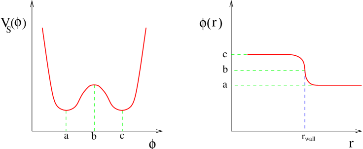
Figure 2.1: The symmetric double well potential, $V_{S}(\phi)$, as a function of $\phi$ (left). The SDWP has two global minima (degenerate vacua) at (a) and (c) and an unstable local maximum at (b). The field configuration shown (right) is a kink profile that interpolates between the two vacua. For $r\ll r_{wall}$ the field is at the vacuum point (c) on the potential, while for $r\gg r_{wall}$ the field is at the vacuum point (a) on the potential; where constant and in the vacuum, the field has no energy. For $r\approx r_{wall}$, the field interpolates between the vacua and must leave the vacuum; the wall therefore has both potential energy and gradient energy. In spherical symmetry the bubble will always collapse since there is only surface tension from the wall and no volume energy within the bubble (due to the degenerate vacua).

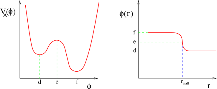
Figure 2.2: The asymmetric double well potential, $V(\phi)$, as a function of $\phi$ (left). The ADWP has two local minima (non-degenerate vacua) at (d) and (f) and an unstable local maximum at (e). Vacuum point (d) is referred to as the false vacuum since it is not the global minimum and is unstable to fluctuations. Vacuum point (f) is referred to as the true vacuum since it is the global minimum and is stable to fluctuations. The field configuration shown (right) is a kink profile that interpolates between the two vacua. For $r\ll r_{wall}$ the field is in the true vacuum, while for $r\gg r_{wall}$ the field is in the false vacuum; where constant and in the vacuum, the field has no energy. For $r\approx r_{wall}$, the field interpolates between the vacua and must leave the vacuum; the wall therefore has both potential energy and gradient energy. In spherical symmetry their is competition between the surface tension trying to make the wall collapse and the volume energy (from the more energetically favorable true vacuum) trying to make the wall expand. The bubble’s fate depends on the balance between the two forces.

The first use of the $\lambda\phi^{4}$ theory to discuss phase transitions is usually credited to Landau and Ginzburg, [36]. The theory is widely applicable and has been used to describe many types of phenomena, ranging from phase transitions in uniaxial ferrolectrics [46], to phase transitions and defect dynamics within superconductors and superfluids [61], to cosmological phase transitions resulting from the spontaneous breakdown of gauge symmetries ([21], [22], [27], [45], [49] [52], and [67], for general treatment; and [35], [37], [38], [60], and [65], for oscillon related studies). Although in this thesis the particle physics and cosmology vernacular is mostly used, the results are applicable to any scalar field model described by the non-linear Klein-Gordon equation with a SDWP or ADWP.

When describing a particle theory, a local minimum describes a vacuum state; the global minimum is the true vacuum while all other minima are false vacua. For the SDWP in figure 2.1, the sample initial data interpolates between the two degenerate vacuum states. For $r>r_{wall}$ the field is in the vacuum state described by point a on the potential, $V(\phi)$, while for $r<r_{wall}$ the field is in the vacuum state described by point c. At and around $r=r_{wall}$, the field interpolates between the two vacuum states and is called a domain wall. Almost all of the energy of the field is concentrated in the wall. There is no potential energy or gradient energy in the field away from $r_{wall}$, since it is in the vacuum; whereas in the wall the field leaves the vacuum, so it has both potential energy and energy due to the gradients of the field. If $r$ is a Cartesian-like coordinate and the field is plane-symmetric then the wall is a planar domain wall. However, if $r$ is a radial (spherical) coordinate, the wall has the shape of a spherical shell, and is often referred to as a bubble wall. The term bubble is in analogy to bubbles in fluids that are created during a change of phase, like gas bubbles forming in liquids, only instead of separating different states of matter, these bubbles separate different vacuum states of a particle theory.

Although the term bubble is used for both SDWP and ADWP alike, the analogy actually is best suited to the ADWP (depicted in figure 2.2). In the ADWP, the bubble wall separates the volume of space in the false vacuum from the volume of space in the more energetically favorable true vacuum. This is exactly like a superheated liquid undergoing a phase transition to a gas, where the false vacuum is the liquid and the true vacuum is the gas. In the liquid-gas transition thermodynamic fluctuations cause gas bubbles to form in the liquid; the fate of the bubbles is determined by the competition between the surface tension in the wall and the volume energy within the bubble wall. For a large enough fluctuation it will be energetically favorable for the bubble wall to continue to expand, thus filling up space with the more energetically favorable gas. This is exactly what happens with vacuum state phase transitions, except instead of thermodynamic fluctuations, the bubbles are usually nucleated by quantum fluctuations.

2.2 The (1+1) plane-symmetric $\left(\phi^{2}-1\right)^{2}$ model

The Klein-Gordon equation in (1+1) dimensions with the SDWP

$${\frac{\partial^{2}\phi}{\partial t}-\frac{\partial^{2}\phi}{\partial x}-\phi+\phi^{3}=0}$$ (2.2)

(where $\phi\equiv\phi(x,t)$) has been studied extensively over the last century. One of the most exciting discoveries was that the model supports solitary waves, stable localized solutions to non-linear field equations. For equation 2.2 these solitary waves take the form

$${\phi(x,t)_{\pm}=\pm{\rm tanh}\left(\frac{\gamma\left(x-vt\right)}{\sqrt{2}}\right)}$$ (2.3)

where $\gamma=1/\sqrt{1-v^{2}}$ and $v$ is the velocity of the kink or antikink (plus or minus sign, respectively). Much of the research of this model was motivated by the attempt to understand particle physics (meson) scattering experiments. In this context, Campbell et al.[10], showed that there is a resonant structure within the kink-antikink parameter space. The possible outcomes (varying depending upon the initial velocity of the kinks, $\pm v_{i}$) were reflection, annihilation, or collapse to a long-lived but unstable bound-state. A resonance between the translational mode of the colliding kinks and their individual internal shape mode vibrations gives rise to a very intricate structure for the endstate as a function of initial velocity. This structure was later shown (in the context of cosmological domain wall collisions) to be fractal in nature, [1]. The fractal structure was found within “$n$-bounce windows”, where the kinks collide, reflect off one another, and then collide again after radiating away energy (the process repeats itself $n$ times).

2.3 What is an Oscillon?

The term oscillon has a few different meanings depending on context, but here it refers to a time-dependent spherically-symmetric coherent localized solution to a non-linear field equation (SDWP or ADWP) which is unstable but long-lived compared to the typical time-scale involved in the problem. Oscillons, originally called pulsons, were first studied numerically with the SDWP in 1977 by Bogolyubskii and Makhankov. They showed that for a wide range of initial data, the behavior of a collapsing bubble was characterized by three stages:

• Collapse: The bubble wall collapses toward $r=0$ and the field oscillates irregularly while radiating a large amount of its initial energy.

• Pseudo-stable Oscillations: The oscillon settles into a state where it remains localized (the location of the bubble wall is bounded) and the field oscillates about the stable vacuum, radiating very little energy. The term pseudo-stable is used because although the oscillons are unstable, they can last for thousands of times longer than the time predicted by linear analysis (which also is roughly the oscillon’s period of oscillation).

• Dispersal: Eventually, an unstable shape-mode triggers the dispersal of the oscillon and the system is left in the original ($r\rightarrow\infty$) vacuum state.

Nearly twenty years later, Copeland et al. [24], performed a much more thorough (and computationally rigorous) investigation of oscillons. Oscillons were shown to be extremely long-lived for a wide range of parameter values for both the SDWP and the ADWP (with varying degrees of asymmetry). The perturbative methods used provided an explanation for two properties of oscillons: A) the existence of a minimum radius for oscillon formation created from static bubble collapse, and B) the need for the initial energy of the field configuration to be above a certain threshold.

Although Copeland, Gleiser, and Müller [24], were the first to really dissect oscillons and to start exploring how and why they behave the way they do, their investigations (as good ones do) raised as many (or more) questions as they answered! In particular, Copeland et al. did not explore the fine structure of the parameter space as [10] and [1] did for the (1+1) plane-symmetric case, nor did they explore what effect non-spherical excitations play on the stability of oscillons. This work explores these two points and others that arose throughout the process.

Chapter 3 Numerical Analysis and MIB Coordinates

This chapter reviews the basic numerical methods (both new and old) employed throughout our research and motivates some of the choices made in the notation and form of the equations used. Although a complete description of finite difference equations, stability analysis, and dissipation are well beyond the scope of this thesis, a basic explanation of one and two dimensional finite difference and dissipation operators is provided. Finally, a new technique which solves problems associated with solving massive field equations on a lattice is introduced here. Implementation of this technique is then detailed in chapters 4 and 5.

3.1 Finite Differences: Definitions and Notation

Since the dawn of calculus in the 17th century, there has been a desire to be able to solve differential (and partial differential) equations. However, for most of the time since Newton and Leibniz, the majority of mathematicians and physicists have been limited to solving differential equations in closed-form or with various types of perturbative methods. These barriers have in large part collapsed since the creation of the computer in the latter part of the 20th century. Faster and faster computers, coupled with new numerical methods, continue to allow people to solve equations that before were far out of their reach. There are a great many numerical methods that have been developed for the solution of partial differential equations (PDEs), including finite differences, finite elements, spectral methods, and more. A brief explanation of finite differences is presented here, focusing on aspects most relevant to this research. (The following subsections are largely based on the class and lecture notes by Choptuik, [17], [19]).

3.1.1 Discretization

For problems such as those considered here, finite differencing provides a very natural and straightforward route to the approximate solution of time-dependent partial-differential equations. A finite difference approximation (FDA) to a partial differential equation (PDE) is obtained by replacing a continuous differential system of equations with a discrete system of approximate equations. The spacetime domain is represented by a discrete number of points on a static uniform mesh that are labeled by $x_{k}$ and $t^{n}$, for integer $k$, $n$. The discretization scale is set by $h\equiv\Delta x=\lambda\Delta t$, and the error associated with the approximation should go to zero as $h$ goes to zero. For a continuum differential system,

$$Lu=f$$ (3.1)

where $L$ is a differential operator, $u$ is the continuous solution, and $f$ is the continuous source function, we use

$$\hat{L}\hat{u}=\hat{f}$$ (3.2)

to denote its finite difference approximation, where $\hat{L}$ is a discrete difference operator, $\hat{u}$ is the discrete solution, and $\hat{f}$ is the discrete source function. Throughout this chapter, $\hat{}$ will denote a discrete quantity; for clarity this notation will be dropped in subsequent chapters and discrete quantities will be recognized by their space and time indexes, $u^{n}_{k}$.

3.1.2 Residual

It is useful to rewrite the FDA above as

$$\hat{L}\hat{u}-\hat{f}=0;$$ (3.3)

for a fully explicit scheme, this equation can be solved exactly. However, for iterative schemes, the right hand side of (3.3) will actually have a non-zero value that is representative of how well $\hat{u}$ solves the system. This leads to the definition of a residual

$$\hat{r}\equiv\hat{L}\tilde{u}-\hat{f},$$ (3.4)

where $\tilde{u}$ is the “instantaneous approximation” of $\hat{u}$, i.e. that which converges to $\hat{u}$ in the limit of infinite iteration. Thus, $\hat{r}$ gives a measure of how well $\hat{u}$ satisfies the FDA, and an iterative scheme is said to be convergent if the residual is driven to zero in the limit.

3.1.3 Truncation and Solution Errors

The truncation error of a finite difference approximation is defined to be

$$\hat{\tau}\equiv\hat{L}u-\hat{f}$$ (3.5)

where we note that the discrete operator $\hat{L}$ acts on the continuum solution $u$. $\hat{\tau}$ often cannot be obtained exactly since the solution $u$ is not usually known.

The solution error is defined to be

$$\hat{e}\equiv u-\hat{u}$$ (3.6)

and is the direct measure of how different the approximate solution $\hat{u}$ is to the continuum solution $u$. Although $u$ must be known exactly to know the exact solution error, an approximate solution error (the solution error to leading order) can usually be obtained numerically (see 3.1.6 below).

3.1.4 Consistency and Order of an FDA

A difference scheme with discretization scale $h$ is a consistent representation of the continuous system if the truncation error goes to zero as the discretization scale goes to zero. Furthermore, the difference scheme is said to be p-th order accurate if

$$\lim_{h\rightarrow 0}\hat{\tau}=O(h^{p})$$ (3.7)

for an integer $p$. All of the schemes in this thesis are second-order, so hereafter it is assumed that $p=2$.

3.1.5 Richardson Expandability

For a centered difference scheme $\hat{L}$, with discretization scale $h$, the solution $u$ is related to the discrete approximation $\hat{u}$ by

$$\hat{u}=u+e_{2}h^{2}+e_{4}h^{4}+\cdots$$ (3.8)

where the $e_{i}$ are h-independent functions. A non-centered scheme will also have odd terms $e_{3}h^{3}$, $e_{5}h^{5}$, etc. Equation 3.8 is referred to as a Richardson expansion.

3.1.6 Convergence

A finite difference approximation is said to be convergent if and only if

$$\hat{\tau}\rightarrow 0\ \ {\rm as}\ \ h\rightarrow 0.$$ (3.9)

Showing convergence is of prime importance in numerical analysis as it is a statement that the solution obtained numerically really approaches the continuum solution as the discretization goes to zero. A useful formula used throughout this thesis describes what is called (by Choptuik) the convergence factor,

$$C_{f}\equiv\displaystyle{\frac{\hat{u}_{4h}-\hat{u}_{2h}}{\hat{u}_{2h}-\hat{u}_{h}}},$$ (3.10)

where $\hat{u}_{4h}$, $\hat{u}_{2h}$, and $\hat{u}_{h}$, are the solutions with discretization scales $4h$, $2h$, and $h$, respectively. Using the expansion (3.8) it can be shown that for second-order approximations $C_{f}\rightarrow 4$ as h$\rightarrow 0$.

3.1.7 Difference Operators

Tables 3.1 and 3.2 contain the one and two dimensional second order difference operators to be used later. They can be derived by Taylor expanding the solution using the discretization scale as the expansion parameter.

Operator	Definition	Expansion
$\Delta^{f}_{r}u^{n}_{i}$	$\left(-3u^{n}_{i}+4u^{n}_{i+1}-u^{n}_{i+2}\right)/\left(2\Delta r\right)$	$\partial_{r}u\big{|}^{n}_{i}+O\left(h^{2}\right)$
$\Delta^{b}_{r}u^{n}_{i}$	$\left(3u^{n}_{i}-4u^{n}_{i-1}+u^{n}_{i-2}\right)/\left(2\Delta r\right)$	$\partial_{r}u\big{|}^{n}_{i}+O\left(h^{2}\right)$
$\Delta_{r}u^{n}_{i}$	$\left(u^{n}_{i+1}-u^{n}_{i-1}\right)/\left(2\Delta r\right)$	$\partial_{r}u\big{|}^{n}_{i}+O\left(h^{2}\right)$
$\Delta_{r^{3}}u^{n}_{i}$	$\left(u^{n}_{i+1}-u^{n}_{i-1}\right)/\left(r^{3}_{i+1}-r^{3}_{i-1}\right)$	$\partial_{r}u\big{|}^{n}_{i}+O\left(h^{2}\right)$
$\Delta_{t}u^{n}_{i}$	$\left(u^{n+1}_{i}-u^{n}_{i}\right)/\Delta t$	$\partial_{t}u\big{|}^{n+\frac{1}{2}}_{i}+O\left(h^{2}\right)$
$\mu^{\rm dis}_{r}u^{n}_{i}$	-$\epsilon_{\rm dis}[6u^{n}_{i}+u^{n}_{i-2}+u^{n}_{i+2}-$	$\left(\Delta r\right)^{3}\partial^{4}_{x}u\big{|}^{n}_{i}+O\left(h^{7}\right)$
	$4\left(u^{n}_{i-1}+u^{n}_{i+1}\right)]/\left(16\Delta t\right)$
$\mu^{\rm ave}_{t}u^{n}_{i}$	$\left(u^{n+1}_{i}+u^{n}_{i}\right)/2$	$u\big{|}^{n+\frac{1}{2}}_{i}+O\left(h^{2}\right)$

Table 3.1: One dimensional two-level FDA operators, $h=\Delta r=\lambda^{-1}\Delta t$.

Operator	Definition	Expansion
$\Delta^{u}_{R}u^{n}_{i,j}$	$\left(-3u^{n}_{i,j}+4u^{n}_{i+1,j}-u^{n}_{i+2,j}\right)/\left(2\Delta R\right)$	$\partial_{R}u\big{|}^{n}_{i,j}+O\left(h^{2}\right)$
$\Delta^{b}_{R}u^{n}_{i,j}$	$\left(3u^{n}_{i,j}-4u^{n}_{i-1,j}+u^{n}_{i-2,j}\right)/\left(2\Delta R\right)$	$\partial_{R}u\big{|}^{n}_{i,j}+O\left(h^{2}\right)$
$\Delta_{R}u^{n}_{i,j}$	$\left(u^{n}_{i+1,j}-u^{n}_{i-1,j}\right)/\left(2\Delta R\right)$	$\partial_{R}u\big{|}^{n}_{i,j}+O\left(h^{2}\right)$
$\Delta_{R^{2}}u^{n}_{i,j}$	$\left(u^{n}_{i+1,j}-u^{n}_{i-1,j}\right)/\left(R^{2}_{i+1}-R^{2}_{i-1}\right)$	$\partial_{R}u\big{|}^{n}_{i,j}+O\left(h^{2}\right)$
$\Delta^{f}_{z}u^{n}_{i,j}$	$\left(-3u^{n}_{i,j}+4u^{n}_{i,j+1}-u^{n}_{i,j+2}\right)/\left(2\Delta z\right)$	$\partial_{z}u\big{|}^{n}_{i,j}+O\left(h^{2}\right)$
$\Delta^{b}_{z}u^{n}_{i,j}$	$\left(3u^{n}_{i,j}-4u^{n}_{i,j-1}+u^{n}_{i,j-2}\right)/\left(2\Delta z\right)$	$\partial_{z}u\big{|}^{n}_{i,j}+O\left(h^{2}\right)$
$\Delta_{z}u^{n}_{i,j}$	$\left(u^{n}_{i,j-1}-u^{n}_{i,j+1}\right)/\left(2\Delta z\right)$	$\partial_{z}u\big{|}^{n}_{i,j}+O\left(h^{2}\right)$
$\Delta_{t}u^{n}_{i,j}$	$\left(u^{n+1}_{i,j}-u^{n}_{i,j}\right)/\Delta t$	$\partial_{t}u\big{|}^{n+\frac{1}{2}}_{i,j}+O\left(h^{2}\right)$
$\mu^{\rm dis}_{R}u^{n}_{i,j}$	-$\epsilon_{\rm dis}[6u^{n}_{i,j}+u^{n}_{i-2,j}+u^{n}_{i+2,j}-$	$\left(\Delta R\right)^{3}\partial^{4}_{R}u\big{|}^{n}_{i,j}+O\left(h^{7}\right)$
	$4\left(u^{n}_{i-1,j}+u^{n}_{i+1,j}\right)]/\left(16\Delta t\right)$
$\mu^{\rm dis}_{z}u^{n}_{i,j}$	-$\epsilon_{\rm dis}[6u^{n}_{i,j}+u^{n}_{i,j-2}+u^{n}_{i,j+2}-$	$\left(\Delta z\right)^{3}\partial^{4}_{z}u\big{|}^{n}_{i,j}+O\left(h^{7}\right)$
	$4\left(u^{n}_{i,j-1}+u^{n}_{i,j+1}\right)]/\left(16\Delta t\right)$
$\mu^{\rm ave}_{t}u^{n}_{i,j}$	$\left(u^{n+1}_{i,j}+u^{n}_{i,j}\right)/2$	$u\big{|}^{n+\frac{1}{2}}_{i,j}+O\left(\Delta t^{2}\right)$

Table 3.2: Two dimensional two-level FDA operators, $h=\Delta R=\Delta z=\lambda^{-1}\Delta t$.

3.2 Dissipation and Stability

Up to this point, there have been no comments made regarding the stability of numerically evolved solutions using finite differences. Much to the dismay of computational physicists, many of the difference schemes one uses to approximate solutions to partial differential equations do not work because they lead to unphysical growing modes. To understand this effect (and how to correct it) consider the discrete analog to the Fourier decomposition of the continuous function $\tilde{\phi}(k,t)=\displaystyle{\frac{1}{\sqrt{2\pi}}\int^{\infty}_{-\infty}e^{-ikx}\ \phi(x,t)dx}$ (for $k$ continuous),

$$\tilde{u}^{n}(\xi)=\displaystyle{\frac{1}{\sqrt{2\pi}}\sum^{\infty}_{m=-\infty}e^{-i\xi m}\ u^{n}_{m}},$$ (3.11)

for $-\pi\leq\xi\leq\pi$ and discrete $m$, [64], [19]. A mode analysis can be performed by inserting the decomposition (3.11) into the difference equation and looking at the behavior of each Fourier mode over time. For linear differential equations, it is straightforward to write the solution to the difference equation in the form $\tilde{u}^{n+1}(k)=\rho\left(\xi\right)\tilde{u}^{n}(k)$, where $\rho$ is a complex function of $\xi$. It is clear that if $|\rho|^{2}>1$ the mode grows over time, if $|\rho|^{2}=1$ the mode remains constant, and if $|\rho|^{2}<1$ the mode decays over time; $|\rho|^{2}$ is referred to here as an amplification factor. A difference equation is dissipative if no modes grow with time and at least one mode decays, while it is nondissipative if the modes neither decay nor grow, or unstable if any of the modes grow with time.

One method commonly used to make unstable schemes stable, or to make nondissipative and dissipative schemes more stable, is to add dissipation. Dissipation can be added in a variety of ways, but we add it to our difference scheme by incorporating higher order spatial derivatives multiplied by the grid spacing to some power, $(\Delta x)^{n}$. Dissipation usually lowers the amplification factor for most modes, and typically affects higher wavenumbers more dramatically. Put another way, the goal is to dampen high frequency modes while maintaining the order of the original difference scheme.

Using the dissipation operators in conjunction with second order CN derivative operators (see table 3.1), the linear advection equation $\left(\partial_{t}-\partial_{x}\right)\phi=0$, can be approximated by the following FDA:

$$\displaystyle{\frac{u^{n+1}_{j}-u^{n}_{j}}{dt}} = \displaystyle{\frac{u^{n+1}_{j+1}-u^{n+1}_{j-1}}{4dx}+\frac{u^{n}_{j+1}-u^{n}_{j-1}}{4dx}}$$ (3.12)

$$\displaystyle{+\frac{\epsilon_{\rm dis}}{16}\left\{6u^{n}_{j}+u^{n}_{j+2}+u^{n}_{j-2}-4\left(u^{n}_{j+2}+u^{n}_{j-2}\right)\right\}}\,.$$

This scheme has an amplification factor $|\rho^{2}|(\xi)$, where

$$\begin{array}[]{rcl}\rho(\xi)&=&\displaystyle{\frac{1+i\displaystyle{\frac{\lambda}{2}}\sin(\xi)-\displaystyle{\frac{\epsilon_{\rm dis}}{8}}\left(3+\cos(2\xi)-4\cos(\xi)\right)}{1-i\displaystyle{\frac{\lambda}{2}}\sin(\xi)}.}\end{array}$$ (3.13)

Plotting $|\rho|^{2}$ as a function of wavenumber, figure 3.1 shows that the CN scheme is nondissipative for $\epsilon=0$ and stable for $\epsilon\leq 1$.

Figure 3.1: Amplification Factors for CN schemes with and without dissipation, where $\epsilon$ is the parameter measuring the amount of dissipation. $\epsilon=0$ corresponds to no dissipation while $\epsilon=1$ completely quenches the modes at the Nyquist limit, $\xi=\pi$. The CN scheme is marginally stable with no dissipation and stable for $\epsilon>0$.

Unfortunately $|\rho|^{2}(\xi)$ is not so easy to compute for general difference schemes. In particular, when the equation is nonlinear the stability of a difference scheme cannot be easily determined (in closed form), even if the derivative operators used are known to be stable in the linear case. We therefore take an empirical approach and include dissipation as needed in order to make the scheme stable. In fact, for evolution equations such as those studied here, the incorporation of dissipation is often essential to the construction of stable schemes.

3.3 Geometry

This work is certainly not the first to explore numerical solutions to massive scalar field equations. The literature is full of work on both massive ($m^{2}\phi^{2}$) and nonlinear ($\epsilon\phi^{3}$, $\lambda\phi^{4}$, $\sin(\phi)$, etc.) potentials in one, two, and even three dimensions, both coupled to gravity and in flatspace [62], [63], [10]. One of the well-known problems with solving the nonlinear or massive Klein-Gordon (KG) equation (even in flatspace) is that there is no closed-form out-going boundary condition. The massive KG equation is simply $\displaystyle{\left(\Box-m^{2}\right)\phi(\vec{x},t)=0}$, which has a dispersion relation $\omega^{2}=k^{2}+m^{2}$. Therefore, the velocity of the outgoing radiation cannot be uniquely determined and a satisfactory outgoing wave condition cannot be applied. While some of the radiation that reaches the outer boundary will leave the computational domain, significant amounts will also be reflected back and can contaminate the solution. If the phenomena being studied is short-lived, the computational domain can be made large enough so that radiation that does get reflected off the outer boundary will not have time to reach the region of interest. However, for long-lived phenomena (like oscillons or some boson stars) one must deal with the outgoing radiation more directly.

Many previously used attempts consist of using an approximate out-going boundary condition and some sort of absorbing region near the outer edge of the grid. [3], [53], [62], and [63] use a sponge filter, which imposes an outgoing radiation condition over a finite portion of the computational domain; this allows outgoing radiation to propagate while attempting to dampen ingoing radiation. However, due to the aforementioned unknown radiation velocity, this is done only approximately and can be susceptible to back-scatter effects. Recently Gleiser et al, [39], have used a method referred to as adiabatic damping, where instead of focusing only on the outgoing radiation (as in the sponge filter methods) with a potential (roughly) of the form $\gamma\left(\vec{x}\right)\left(\dot{\phi}+\phi^{\prime}\right)$, they use a term of the form $\gamma\left(\vec{x}\right)\dot{\phi}$ and dampen all scalar radiation. However, by adding explicit damping terms to the equations of motion (as opposed to higher order dissipation added to the difference equations) neither of the resulting difference schemes actually reduce to the true equations of motion in the limit that the grid spacing goes to zero.

This section introduces a new geometric technique that effectively absorbs outgoing radiation, has difference equations that reduce to the differential equations in the continuum limit, and that is natural and straightforward to implement in both spherical and axial symmetry. The method employed has two parts, the transformation of coordinates and the incorporation of dissipation into the numerical scheme. The coordinate system used leaves the interior of the grid alone, while transforming the coordinates of the exterior points to be moving outward at approximately the speed of light relative to the interior or original rest frame; the coordinates are monotonically increasingly boosted (MIB). Characteristic analysis of the wave equation (in MIB coordinates) shows that both ingoing and outgoing characteristic velocities approach zero in a region near the outer edge of the grid [20]. As the field slows down it becomes compressed; since the dissipation becomes stronger with increasing wavenumber, the field is quenched. This is shown to occur in a stable and non-reflective manner in (1+1) spherical symmetry and (2+1) axisymmetry.

3.3.1 Radial MIB Coordinates

In spherical symmetry, the outgoing radiation is frozen-out by introducing a new radial coordinate that smoothly interpolates between the standard polar radial coordinate $\tilde{r}$ on Minkowski space

$$d\tilde{s}^{2}=-d\tilde{t}^{2}+d\tilde{r}^{2}+\tilde{r}^{2}d\tilde{\Omega}^{2},$$ (3.14)

(where $d\tilde{\Omega}^{2}=d\tilde{\theta}^{2}+\sin^{2}\tilde{\theta}\,d\tilde{\phi}^{2}$), and an outgoing null coordinate. We define

$$\begin{array}[]{cccc}\tilde{t}=t,&\tilde{r}=r+f(r)t,&{\rm and}&\tilde{\Omega}=\Omega\\ \end{array}$$ (3.15)

where $f(r)$ is a monotonically increasing function that interpolates between $0$ and approximately 1 at some characteristic cutoff, $r_{\rm c}$,

$$f(r)\simeq\left\{\begin{array}[]{rcr}0&{\rm for}&r\ll r_{\rm c}\\ \sim 1&{\rm for}&r\gg r_{\rm c}\end{array}\right\}.$$ (3.16)

In general, these coordinates are not good coordinates everywhere. However, if $f(r)$ is monotonically increasing, the determinant of the Jacobian of the transformation is non-zero for all $t>-\max|f^{\prime}(r)|$ and the coordinate transformation is one-to-one. Although a coordinate singularity inevitably forms as $t$ approaches past timelike infinity, this has no effect on the forward evolution of initial data specified at $t=0$. We must also demand that $f(0)\!=\!0$ to maintain the condition for elementary flatness at the origin. This coordinate choice takes the metric to

$$\begin{array}[]{rcl}ds^{2}&=&\left(-1+f^{2}(r)\right)dt^{2}+2f(r)\left(1+f^{\prime}(r)t\right)dtdr\\ &&+\left(1+f^{\prime}(r)t\right)^{2}dr^{2}+\left(r+f(r)t\right)^{2}d\Omega^{2}\end{array}$$ (3.17)

or in a more familiar (3+1) form ([2],[12],[16]) to

$$ds^{2}=\left(-\alpha^{2}+a^{2}\beta^{2}\right)dt^{2}+2a^{2}\beta dtdr+a^{2}dr^{2}+r^{2}b^{2}d\Omega^{2},$$ (3.18)

where

$$\begin{array}[]{rclcrcl}a(r,t)&\equiv&1+f^{\prime}(r)t&&b(r,t)&\equiv&\displaystyle{1+f(r)\frac{t}{r}}\\ \vspace{-0.275in}\hfil\\ \alpha(r,t)&\equiv&1&&\beta(r,t)&\equiv&\displaystyle{\frac{f(r)}{1+f^{\prime}(r)t}}.\\ \end{array}$$ (3.19)

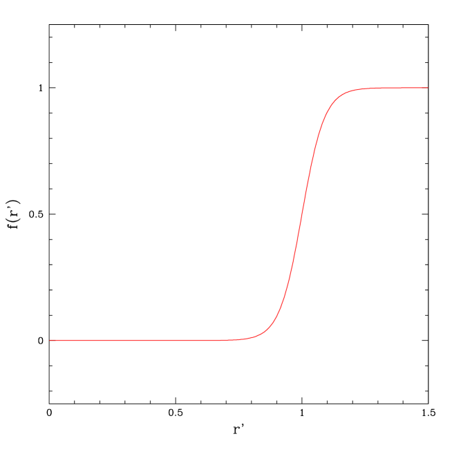
Figure 3.2: Interpolating function, $f(r^{\prime})$, for radial MIB coordinates, where $r^{\prime}$ is in units where $r_{c}=1$. $\delta$ is taken to be $\delta\rightarrow\delta/r_{c}\approx 0.0893$ (corresponding to the system to be used in chapter 4). Wherever $f=0$, the new radial coordinate is left unchanged with respect to the old coordinate, $\tilde{r}$. Where $f>0$ the new radial coordinate is being “shifted” with respect to $\tilde{r}$ with velocity $\beta=f/(1+f^{\prime}t)$.

Assuming the following specific form for $f$ (see figure 3.2):

$$f(r)=\left[1+\tanh\left(\left(r-r_{c}\right)/\delta\right)\right]/2+\epsilon(r_{c},\delta)\,,$$ (3.20)

where $\epsilon(r_{c},\delta)=-\left[1+\tanh\left(\left(-r_{c}\right)/\delta\right)\right]/2$,

Figure 3.3: Plot of the characteristic velocities as a function of $r^{\prime}$ and $t^{\prime}$, where $r^{\prime}$ and $t^{\prime}$ are radial MIB coordinates in units where $r_{c}$ is set to unity, and $\lambda_{+}$ and $\lambda_{-}$ are the outgoing and ingoing characteristics, respectively. $\delta$ is taken to be $\delta\rightarrow\delta/r_{c}\approx 0.0893$ (corresponding to the system to be used in chapter 4). Characteristic velocities are plotted for times $t^{\prime}=0$, $1$, $10$, and $100$ ($t^{\prime}=100$ is larger than the lifetime of the longest lived solution studied in this work). Both characteristic velocities approach zero around $r^{\prime}=1$ as $1/{t^{\prime}}$.

Figure 3.4: Plot of characteristic velocites, $\lambda_{\pm}(r^{\prime},100)$, where $r^{\prime}$ and $t^{\prime}$ are radial MIB coordinates in units where $r_{c}$ is set to unity, and $\lambda_{+}$ and $\lambda_{-}$ are the outgoing and ingoing characteristics, respectively. $\delta$ is taken to be $\delta\rightarrow\delta/r_{c}\approx 0.0893$ (corresponding to the system to be used in chapter 4), and $t^{\prime}=100$ is larger than the lifetime of the longest lived solution discussed in this thesis. Both characteristic velocities approach zero around $r^{\prime}=1$ as $1/{t^{\prime}}$.

we can obtain the actual metric variables, the characteristic velocities, and the conformal structure of the new hypersurfaces.

The characteristic analysis of the Klein-Gordon equation with metric (3.18) yields characterstics

$$\lambda_{\pm}=-\beta\pm\frac{\alpha}{a},$$ (3.21)

where $\lambda_{+}$ and $\lambda_{-}$ are the outgoing and ingoing characteristics, respectively [12], [25]. The MIB system behaves like the old ($\tilde{t}$,$\tilde{r}$) coordinates for $r\ll r_{\rm c}$, but the outgoing radiation gets frozen out in the $r\approx r_{\rm c}$ region. Figure 3.3 and equations (3.21) and (3.19) show that around $r\approx r_{c}$, both the ingoing and the outgoing characteristic velocities go to zero as $t\rightarrow\infty$ (as the inverse power of $t$). It is this property that is responsible for the “freezing-out” of the outgoing radiation [20]. We call these coordinates ($t$,$r$) monotonically increasingly boosted (MIB) radial coordinates.

The conformal structure (figure 3.5) is obtained by applying equations (3.15) to the standard conformal compactification on Minkowski space, $\tilde{t}\pm\tilde{r}=\tan\left(\frac{T\pm R}{2}\right)$ (where here $T$ and $R$ are the axes in the conformal diagram, see [43] or [66]), and then plotting curves of constant $r$ and $t$.

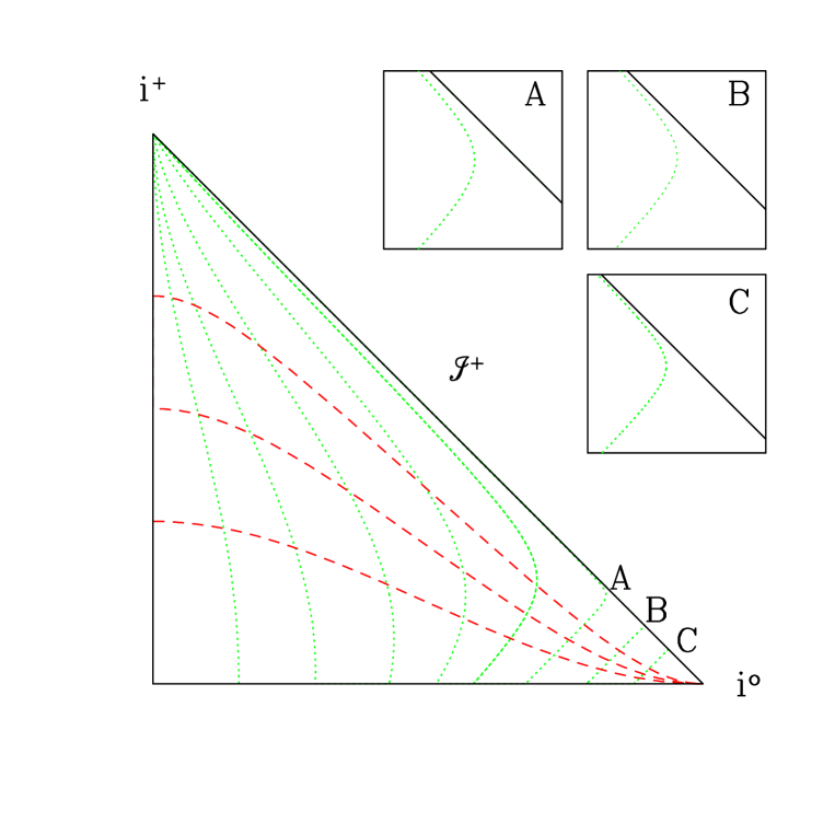
Figure 3.5: Conformal diagram showing surfaces of constant $r$ (dotted lines) and lines of constant $t$ (dashed lines). Lines of constant $t$ look exactly like the constant-$t$ hypersurfaces of Minkowski space, whereas the lines of constant $r$ behave much differently. For $r>r_{c}$, it appears as if the constant-$r$ surfaces are null. This occurs since the coordinates are being shifted outwards at nearly the speed of light. However, as insets A, B, and C show, the constant-$r$ lines do not become null (do not intersect future null infinity), and are everywhere timelike. This is actually easy to understand as the radial coordinate is never moved out at the speed of light (not even at spatial infinity, because of the $\epsilon$ term in equation 3.20).

The constant-$t$ hypersurfaces are everywhere spacelike, and all reach spatial infinity, ${\rm i^{o}}$. Although constant-$r$ surfaces for $r>r_{\rm c}$ appear at first glance to be null (or as if $\left(\frac{\partial}{\partial t}\right)^{a}$ “tips over” to become a null vector), closer examination (see insets of Fig. 3.5) reveals that they are indeed everywhere timelike and do not reach future null infinity, ${\mathcal{J}^{+}}$. This behaviour follows from the fact that the interpolating function, $f(r)$, only reaches unity asymptotically, at ${\rm i^{o}}$.

3.3.2 Axi-Symmetric (2-D) MIB Coordinates

The (1-D) MIB coordinates introduced in the previous subsection also have a straightforward implementation in two dimensions. The (2-D) problems discussed in this work all model (3+1) dimensional spacetimes with axial symmetry. (2-D) MIB coordinates are obtained by again starting from the Minkowski metric, but now in cylindrical coordinates

$$d\tilde{s}^{2}=-d\tilde{t}^{2}+d\tilde{R}^{2}+\tilde{R}^{2}d\tilde{\theta}^{2}+d\tilde{z}^{2}.$$ (3.22)

These coordinates are modified just like the radial coordinate in spherical symmetry (section 3.3.1), except now both the axisymmetric coordinates $R$ and $z$ interpolate between the old ($\tilde{R}$,$\tilde{z}$) coordinates and “null coordinates at ${\rm i^{o}}$”:

$$\begin{array}[]{ccccc}\tilde{t}=t,&\tilde{R}=R+f(R)t,&\tilde{z}=z+g(z)t,&{\rm and}&\tilde{\theta}=\theta\,.\\ \end{array}$$ (3.23)

Here, $f(R)$ and $g(z)$ are monotonically increasing functions: $f(R)$ interpolates between (approximately) $0$ and $1$ at a characteristic cutoff, $R_{c}$; $g(z)$ interpolates (approximately) between $-1$ and $1$ at characteristic cutoffs, $\pm z_{c}$,

$$\begin{array}[]{lcr}f(R)\simeq\left\{\begin{array}[]{rcc}0&{\rm for}&R\ll R_{c}\\ 1&{\rm for}&R\gg R_{c}\end{array}\right\}&&g(z)\simeq\left\{\begin{array}[]{rcc}-1&{\rm for}&z\ll-z_{c}\\ 0&{\rm for}&-z_{c}<z<z_{c}\\ 1&{\rm for}&z\gg z_{c}\end{array}\right\}.\par\end{array}$$ (3.24)

This coordinate choice takes the metric to

$$\begin{array}[]{rcl}ds^{2}&=&\left(-1+f(R)^{2}+g(z)^{2}\right)dt^{2}+2f(R)\left(1+\partial_{R}f(R)t\right)dtdR\\ &&+2g(Z)\left(1+\partial_{z}g(z)t\right)dtdz+\left(1+\partial_{R}f(R)t\right)^{2}dR^{2}\\ &&+\left(R+f(R)t\right)^{2}d\theta^{2}+\left(1+\partial_{z}g(z)t\right)^{2}dz^{2}\end{array}$$ (3.25)

or in a more familiar (3+1) form to

$$\begin{array}[]{rcl}ds^{2}&=&\left(-\alpha^{2}+a^{2}{\beta^{R}}^{2}+b^{2}{\beta^{z}}^{2}\right)dt^{2}+2a^{2}\beta^{R}dtdR+2b^{2}\beta^{Z}dtdZ\\ &&+a^{2}dR^{2}+\tilde{R}^{2}d\theta^{2}+b^{2}dz^{2},\end{array}$$ (3.26)

where

$$\begin{array}[]{rclcrcl}a(R,t)&=&1+\partial_{R}f(R)t&&b(z,t)&=&1+\partial_{z}g(z)t\\ \vspace{-0.5cm}\hfil\\ \beta^{R}(R,t)&=&\displaystyle{\frac{f(R)}{1+\partial_{R}f(R)t}}&&\beta^{z}(z,t)&=&\displaystyle{\frac{g(z)}{1+\partial_{z}g(z)t}\vspace{0.25cm}}\\ \alpha(R,t)&=&1&&\tilde{R}(R,t)&=&R+f(R)t.\end{array}$$ (3.27)

In accordance with (3.24), the interpolating functions, $f$ and $g$, are taken to be

$$f(R) = \left[1+\tanh\left(\left(R-R_{c}\right)/\delta_{R}\right)\right]/2+\epsilon(R_{c},\delta_{R})$$ (3.28)

$$g(z) = \tanh\left(\left(z-z_{c}\right)/\delta_{z}\right)/2+\tanh\left(\left(z+z_{c}\right)/\delta_{z}\right)/2,$$ (3.29)

where $\epsilon(R_{c},\delta_{R})=-\left[1+\tanh\left(\left(-R_{c}\right)/\delta_{R}\right)\right]/2$, (see Figure 3.6).

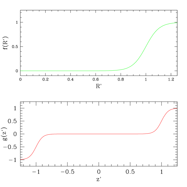
Figure 3.6: Interpolating functions, $f(R^{\prime})$ and $g(z^{\prime})$, for axisymmetric MIB coordinates, where $R^{\prime}$ and $z^{\prime}$ are in units where $R_{c}$ and $z_{c}$ are equal to one. $\delta_{R}$ and $\delta_{z}$ are taken to be approximately $0.1067$ (corresponding to the system to be used in chapter 5). Wherever $f=0$, the new radial coordinate, $R$, is left unchanged with respect to the old coordinate, $\tilde{R}$. For $f>0$ the new radial coordinate is being shifted outward with respect to $\tilde{R}$ with velocity $\beta^{R}=f/(1+\partial_{R}ft)$. Wherever $g(z^{\prime})=0$, the new $z$ coordinate is left unchanged with respect to the old coordinate $\tilde{z}$. For $g>0$ the $z$ coordinate is being shifted outward with respect to $\tilde{z}$ with velocity $\beta^{z}=g/(1+\partial_{z}gt)$; note however that the sign of $g$ (and consequently $\beta^{z}$) is negative for $z<0$ as the coordinate is moving outward toward more negative z.

Figure 3.7: Plot of the characteristic velocities, $\lambda^{R}_{\pm}$, as a function of $R^{\prime}$ and $t^{\prime}$, where $R^{\prime}$ and $t^{\prime}$ are axisymmetric MIB coordinates where $R_{c}$ is set to unity, and $\lambda_{+}$ and $\lambda_{-}$ are the outgoing and ingoing characteristics, respectively. $\delta$ is taken to be $\delta_{r}\rightarrow\delta_{r}/R_{c}\approx 0.1067$ (corresponding to the system to be used in chapter 5). Characteristic velocities are plotted for times $t^{\prime}=0$, $1$, $10$, and $100$, and where $t^{\prime}=100$ is larger than the lifetime of the longest of the longest lived solution studied in this work. Both characteristic velocities approach zero around $r^{\prime}=1$ as $1/{t^{\prime}}$.

Figure 3.8: Plot of the characteristic velocities, $\lambda^{z}_{\pm}$, as a function of $z^{\prime}$ and $t^{\prime}$, where $z^{\prime}$ and $t^{\prime}$ are axisymmetric MIB coordinates where $z_{c}$ is set to unity, and $\lambda_{+}$ and $\lambda_{-}$ are the outgoing and ingoing characteristics, respectively. $\delta_{z}$ is taken to be $\delta_{z}\rightarrow\delta_{z}/z_{c}\approx 0.1067$ (corresponding to the system to be used in chapter 5). Characteristic velocities are plotted for times $t^{\prime}=0$, $1$, $10$, and $100$ ($t^{\prime}=100$ is larger than the lifetime of the longest lived solution studied in this work). Both characteristic velocities approach zero around $z^{\prime}=\pm 1$ as $1/{t^{\prime}}$.

Figure 3.9: Plot of the characteristic velocities, $\lambda^{z}_{\pm}$, as a function of $z^{\prime}$ and $t^{\prime}$, where $z^{\prime}$ and $t^{\prime}$ are axisymmetric MIB coordinates where $z_{c}$ is set to unity, and $\lambda_{+}$ and $\lambda_{-}$ are the outgoing and ingoing characteristics, respectively. $\delta_{z}$ is taken to be $\delta_{z}\rightarrow\delta_{z}/z_{c}\approx 0.1067$ (corresponding to the system to be used in chapter 5). Characteristic velocities are plotted for times $t^{\prime}=0$, $1$, $10$, and $100$ ($t^{\prime}=100$ is larger than the lifetime of the longest lived solution studied in this work). Both characteristic velocities approach zero around $z^{\prime}=\pm 1$ as $1/{t^{\prime}}$.

The characteristics of the system are

$$\lambda^{R}_{\pm} = -\beta^{R}\pm 1/a$$ (3.30)

$$\lambda^{z}_{\pm} = -\beta^{z}\pm 1/b,$$ (3.31)

where $\lambda^{R}_{\pm}$ and $\lambda^{z}_{\pm}$ are the characteristics in the $R$ and $z$ directions, respectively. As with the spherically symmetric case, the system behaves like the old ($\tilde{R}$, $\tilde{z}$, and $\tilde{t}$) coordinates for $R<R_{c}$ and $-z_{c}<z<z_{c}$, while around $R\approx R_{c}$ and $z\approx\pm z_{c}$, the characteristic velocities, $\lambda^{R}_{\pm}\rightarrow 0$ and $\lambda^{z}_{\pm}\rightarrow 0$, as $t\rightarrow\infty$ (as the inverse power of $t$). This again has the effect of freezing-out the outgoing radiation.

Figure 3.10: Plot of characteristic velocites, $\lambda_{\pm}(R^{\prime},100)$, where $R^{\prime}$ and $t^{\prime}$ are axisymmetric MIB coordinates in units where $R_{c}$ is set to unity, and $\lambda_{+}$ and $\lambda_{-}$ are the outgoing and ingoing characteristics, respectively. $\delta$ is taken to be $\delta\rightarrow\delta/R_{c}\approx 0.1067$ (corresponding to the system to be used in chapter 5), and $t^{\prime}=100$ is larger than the lifetime of the longest lived solution discussed in this thesis. Both characteristic velocities approach zero around $r^{\prime}=1$ as $1/{t^{\prime}}$.

Figure 3.11: Plot of characteristic velocites, $\lambda_{\pm}(z^{\prime},100)$, where $z^{\prime}$ and $t^{\prime}$ are axisymmetric MIB coordinates in units where $z_{c}$ is set to unity, and $\lambda_{+}$ and $\lambda_{-}$ are the outgoing and ingoing characteristics, respectively. $\delta$ is taken to be $\delta\rightarrow\delta/z_{c}\approx 0.1067$ (corresponding to the system to be used in chapter 5), and $t^{\prime}=100$ is larger than the lifetime of the longest lived solution discussed in this thesis. Both characteristic velocities approach zero around $r^{\prime}=1$ as $1/{t^{\prime}}$.

3.4 Dissipation & MIB Coordinates Working Together

The primary reason dissipation was introduced and stressed in this chapter is because it is integral to the stability of the MIB scheme. Since MIB coordinates cause all the outgoing radiation to accumulate in a very small region of the grid (creating large gradients in the fields), when MIB coordinates are used without dissipation the scheme is always unstable. However, with dissipation the field is quenched in a stable and non-reflective manner. This can happen because the amplification factor for the Crank-Nicholson scheme (analagous to that seen in figure 4.2) is significantly less than one for high frequency solution components. Therefore, the more the radiation gets spatialy compressed, the more it is dissipated. Details of this process are discussed in chapter 4 in the context of spherically collapse.

Note that although the above explanation is self-consistent and explains how the system can be stable, it certainly provides no convincing argument that the scheme should be stable (or non-reflective for that matter). In fact, many techniques explored throughout the creation of the one discussed here were very unstable and reflected significant amounts of radiation! In addition to the sponge-filter approach (mentioned in section 3.3), there has been much research devoted to the study of outgoing radiation and outgoing boundary conditions. For the sake of completeness, we briefly review some of this research here.

Cauchy-Characteristic Matching (CCM) is a way to solve Einstein’s Equations that matches typical Cauchy evolution on the interior of the computational domain to characteristic evolution on the exterior, [4]. The original motivation was to measure the outgoing radiation that reaches null infinity, however, in the process the method eliminates the need for an outgoing radiation boundary condition. The technique was developed for massless radiation although some success has been made recently with the incorporation of matter [5], [51]. CCM is reported to be more efficient than previously used techniques, but still requires separate evolution of two domains and calculations to match them together; the methods employed here involve a single Cauchy evolution.

Null-cone evolution [41] and other purely characteristic evolution techniques (ie. where the entire evolution is performed in characteristic coordinates, [40], [69]), have also been successful in numerical relativity and seemed like a very promising way to evolve the nlKG equation. Unfortunately, using characteristic coordinates with a truncated grid is still problematic due to the lack of a satisfactory outgoing boundary condition. However, unlike typical ($r$,$t$) coordinates, compactification is natural with null evolution and generally preserves the smoothness properties of radiation [69]. Furthermore, in compactified characteristic coordinates exact boundary conditions can be set on the outer boundary of the grid, $\mathcal{J}^{+}$. Numerical implementations can usually be evolved stably and radiation can be measured at $\mathcal{J}^{+}$. However, this tends to work well only for radiation that travels along null characteristics (ie. massless fields). When the fields are massive the field does not propagate along null characteristics (and therefore does not reach null infinity), and there is either leakage out to ${\mathcal{J}^{+}}$ of massive field, or instabilities that arise from steep gradients due to compression of the outgoing radiation, [70].

Similar problems occur evolving massive radiation with the conformal compactification methods developed by Friedrich, [34], and implemented numerically by Hubner, [44] and Frauendiener, [28], [29], [30]; the conformal compactification of the spacetime brings null infinity to the outermost grid point and still causes problems with massive radiation [44].

Chapter 4 Spherically Symmetric Oscillons

4.1 The Klein-Gordon Equation in MIB Coordinates with SDWP

In this chapter we introduce the notation, equations of motion, and discuss results from a computer code which uses spherically symmetric MIB coordinates.

We are interested in massive scalar field theory described by the (1+1) spherically symmetric action

$$S[\phi]=\int d^{4}x\sqrt{|g|}\left(-\frac{1}{2}g^{\mu\nu}\nabla_{\mu}\phi\nabla_{\nu}\phi-V(\phi)\right)$$ (4.1)

where $\phi\equiv\phi(r,t)$, $V(\phi)$ is a symmetric double well potential (see figure 4.1), $\displaystyle{V_{S}(\phi)=\frac{1}{4}\left(\phi^{2}-1\right)^{2}}$, $g_{\mu\nu}$ is the flatspace metric in spherically symmetric MIB coordinates, (3.18), and $g$ is the determinant of $g_{\mu\nu}$.

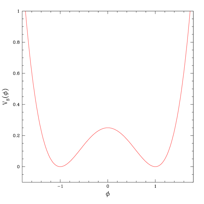
Figure 4.1: Symmetric double well potential, $\displaystyle{V_{S}(\phi)=\frac{1}{4}\left(\phi^{2}-1\right)^{2}}$. The potential has two degenerate minima at $\phi=\pm 1$ and an unstable local maximum at $\phi=0$. See figure 2.1 for detailed description of features and interpretation of kink profile (bubble) initial data.

The equation of motion for the action (4.1) is

$$\frac{1}{\sqrt{|g|}}\partial_{\mu}\left(\sqrt{|g|}g^{\mu\nu}\partial_{\nu}\phi\right)=\phi\left(\phi^{2}-1\right)$$ (4.2)

which with (3.18), (3.19), and the definitions

$$\Pi(r,t) \equiv \frac{a}{\alpha}\left(\partial_{t}{\phi}-\beta\partial_{r}\phi\right),$$ (4.3)

$$\Phi(r,t) \equiv \partial_{r}\phi,$$ (4.4)

yields

$$\dot{\Pi} = \frac{1}{r^{2}b^{2}}\left(r^{2}b^{2}\left(\frac{\alpha}{a}\Phi+\beta\Pi\right)\right)^{\prime}-2\frac{\dot{b}}{b}\Pi-\alpha a\phi\left(\phi^{2}-1\right)$$ (4.5)

$$\dot{\Phi} = \left(\frac{\alpha}{a}\Pi+\beta\Phi\right)^{\prime}$$ (4.6)

$$\dot{\phi} = \frac{\alpha}{a}\Pi+\beta\Phi$$ (4.7)

where  $\dot{}\equiv\partial_{t}$ and  ${}^{\prime}\equiv\partial_{r}$. These equations are the familiar (3+1) form for the spherically symmetric Klein-Gordon field coupled to gravity. However, instead of having a truly dynamical geometry, here $a(r,t)$, $b(r,t)$, $\alpha(r,t)$, and $\beta(r,t)$ are known functions of $(r,t)$, which result from the MIB coordinate transformation of flatspace.

4.2 Finite Difference Equations

Equations (4.5,4.6,4.7) are solved using two-level second order (in both space and time) finite difference approximations on a static uniform grid with $N_{r}$ grid points. The scale of discretization is set by $\Delta r$ and $\Delta t=\lambda\Delta r$, where we fixed the Courant factor, $\lambda$, to $0.5$ as we changed the base discretization.

Using the operators from Table 3.1, $\partial_{r}\tilde{r}=a$, $\partial_{r}=nr^{n-1}\partial_{r^{n}}$, and $rb=\tilde{r}$, the interior difference equations ($3\leq i\leq N_{r}-2$) are

$$\displaystyle{\Delta_{t}\Pi^{n}_{i}} = \displaystyle{3\mu_{t}\left[a\Delta_{\tilde{r}^{3}}\left(\tilde{r}^{2}\left(\frac{\alpha}{a}\Phi+\beta\Pi\right)\right)\right]^{n}_{i}}$$ (4.8)

$$\displaystyle{-2\mu_{t}\left(\frac{\dot{b}}{b}\Pi-\alpha a\phi\left(\phi^{2}-1\right)\right)^{n}_{i}}+\mu_{t}^{\rm diss}\Pi^{n}_{i},$$

$$\Delta_{t}\Phi^{n}_{i} = \mu_{t}\Delta_{r}\left(\frac{\alpha}{a}\Pi+\beta\Phi\right)^{n}_{i}+\mu_{t}^{\rm diss}\Phi^{n}_{i},$$ (4.9)

$$\Delta_{t}\phi^{n}_{i} = \mu_{t}\left(\frac{\alpha}{a}\Pi+\beta\Phi\right)^{n}_{i}+\mu_{t}^{\rm diss}\phi^{n}_{i}.$$ (4.10)

and include dissipation. On the two grid points adjacent to the boundaries, $i=2$ and $i=N_{r}-1$, the same equations are solved without dissipation (since the two points needed on either side are unavailable):

$$\displaystyle{\Delta_{t}\Pi^{n}_{i}} = \displaystyle{3\mu_{t}\left[a\Delta_{\tilde{r}^{3}}\left(\tilde{r}^{2}\left(\frac{\alpha}{a}\Phi+\beta\Pi\right)\right)\right]^{n}_{i}}$$ (4.11)

$$\displaystyle{-2\mu_{t}\left(\frac{\dot{b}}{b}\Pi-\alpha a\phi\left(\phi^{2}-1\right)\right)^{n}_{i}},$$

$$\Delta_{t}\Phi^{n}_{i} = \mu_{t}\Delta_{r}\left(\frac{\alpha}{a}\Pi+\beta\Phi\right)^{n}_{i},$$ (4.12)

$$\Delta_{t}\phi^{n}_{i} = \mu_{t}\left(\frac{\alpha}{a}\Pi+\beta\Phi\right)^{n}_{i}.$$ (4.13)

These equations are solved using an iterative scheme, which is iterated until the $\ell_{2}$-norms of the solutions at $t^{n+1}$ converge to one part in $10^{8}$, where the $\ell_{2}$-norm is defined for a vector $x_{i}$ to be

$${||{\bf{{\hbox{\bfgreek\char 120\relax}}}}||_{2}=\left(\frac{1}{N}\sum^{N}_{i}|x_{i}|^{2}\right)^{1/2}}$$ (4.14)

Since the functions $a$, $b$, $\dot{b}$, $\alpha$, $\beta$, and $\tilde{r}$ are explicitly known functions, when discretized we simply evaluate the given function at $r_{i}=(i-1)\Delta r$ and $t^{n}=(n-1)\Delta t$. On the inner ($r=0$) boundary we applied conditions necessary for regularity at the origin:

$$\Phi^{n}_{i}=0$$ (4.15)

$$\mu_{t}\left(\Delta^{f}_{i}\Pi-\displaystyle{\frac{a^{\prime}}{a}\Pi}\right)^{n}_{i}=0$$ (4.16)

where (4.15) is a statement of regularity in the scalar field, and (4.16) results from equation (4.13) and the commutation of partial derivatives. The field $\phi$ is evolved using

$$\Delta_{t}\phi=\mu_{t}\left(\frac{\alpha\Pi}{a}+\beta\Phi\right)^{n}_{i}.$$ (4.17)

For the outer boundary, our choice of equations makes very little difference since the physical radial position ($\tilde{r}$) corresponding to the outermost point is moving out at nearly the speed of light, therefore none of the outgoing field ever reaches this gridpoint. Nevertheless, we employed the typical massless scalar field outgoing boundary condition for $\Pi$ and $\Phi$, and evolved $\phi$ with its equation of motion:

$$\Delta_{t}\Pi^{n}_{i}+\mu_{t}\left(\Delta^{b}_{r}\Pi+\frac{\Pi}{r}\right)^{n}_{i}=0,$$ (4.18)

$$\Delta_{t}\Phi^{n}_{i}+\mu_{t}\left(\Delta^{b}_{r}\Phi+\frac{\Phi}{r}\right)^{n}_{i}=0,$$ (4.19)

$$\Delta_{t}\phi=\mu_{t}\left(\frac{\alpha\Pi}{a}+\beta\Phi\right)^{n}_{i}.$$ (4.20)

4.3 Testing the MIB Code

One might think that freezing out the outgoing radiation while keeping a static uniform mesh would lead to a “bunching-up” of the outgoing radiation from the oscillating source which would cause a loss of resolution, numerical instabilities, and eventually crash the code. However, as already discussed, this turns out not to be the case; all outgoing radiation is stably “frozen-out” around $r\approx r_{\rm c}$ and the steep gradients that should form in this region are smoothed out and quenched by the dissipation (see figure 4.2). As the oscillations approach $r\approx r_{c}$ their wavenumber approaches the Nyquist limit, $\xi\rightarrow\pi$, and since the amplification factor for these modes is significantly less than one they are rapidly quenched (analogously to the solution of the advection equation using the CN scheme shown in figure 3.1). Put simply, the coordinate system causes the oscillations to “bunch-up”, while the higher-order dissipation quenches the resultant high-frequency modes.

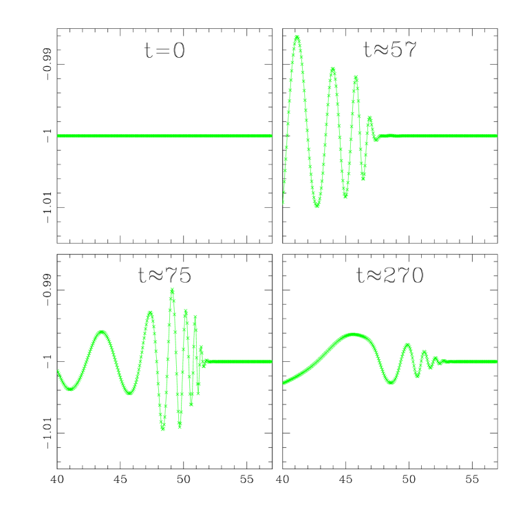
Figure 4.2: Fundamental field $\phi(r)$ in the freeze-out region (cutoff actually at $r_{c}=56$) at $t=0,\ 57,\ 75,\ {\rm and}\ 270$. As the characteristic velocities of the radiation go to zero around $r_{c}$ (as seen in figure 3.4), the wavelength of the radiation is shortened to the Nyquist limit on the lattice, $2\Delta r$. The higher-order dissipation added to the system is responsible for quenching the field; figure 3.1 shows the amplification factor $|\rho|^{2}$ as a function of wavenumber is significantly less than one as the wavenumber approaches the Nyquist limit (the plot of $|\rho(\xi)|^{2}$ is actually for the advection equation, but is qualitatively similar).

There is a loss of resolution and second order convergence directly around $r_{\rm c}$, but this does not affect stability or convergence of the solution for $r\ll r_{\rm c}$. Figure (4.3) shows a convergence test for the field $\phi$ for $r<r_{\rm c}/2$ over roughly six crossing times.

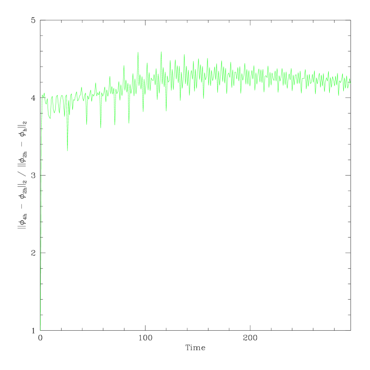
Figure 4.3: Convergence factor, $C_{f}=||\phi_{4h}-\phi_{2h}||_{2}/||\phi_{2h}-\phi_{h}||_{2}$, for the field $\phi$ composed from the solution at three different discretizations (value of 4 indicates 2nd order convergence, as shown in section 3.1.6).

Since we are solving equation (4.2) in flatspace, it is very simple to monitor energy conservation. The spacetime admits a timelike Killing vector, $t^{\nu}$, so we have a conserved current, $J_{\mu}\equiv t^{\nu}T_{\mu\nu}$. We monitor the flux of $J_{\mu}$ through a gaussian surface constructed from two adjacent spacelike hypersurfaces for $r\leq r_{\rm c}$ (with normals $n_{\mu}=(\pm 1,0,0,0)$), and an “endcap” at $r=r_{\rm endcap}$ (with normal $n_{r}^{\mu}=(0,a^{-1},0,0))$. To obtain the the conserved energy at a time, $t$, the energy contained in the bubble,

$$E_{\rm bubble}(t)=4\pi\int\limits_{0}^{\ \ \ r_{endcap}}r^{2}b^{2}\left(\frac{\Pi^{2}+\Phi^{2}}{2a^{2}}+V(\phi)\right)dr,$$ (4.21)

(where the integrand is evaluated at time $t$) is added to the total radiated energy,

$$E_{\rm rad}(t)=4\pi\int\limits_{0}^{\ t}r^{2}b^{2}\frac{\Pi\Phi}{a^{2}}dt^{\prime}$$ (4.22)

(where the integrand is evaluated at $r=r_{\rm endcap}$). The sum, $E_{\rm total}=E_{\rm bubble}+E_{\rm rad}$, remains conserved to within a few tenths of a percent through almost two thousand oscillation periods ($t\approx 8000m^{-1}$ or up to a quarter million iterations, see Fig. (4.4)).

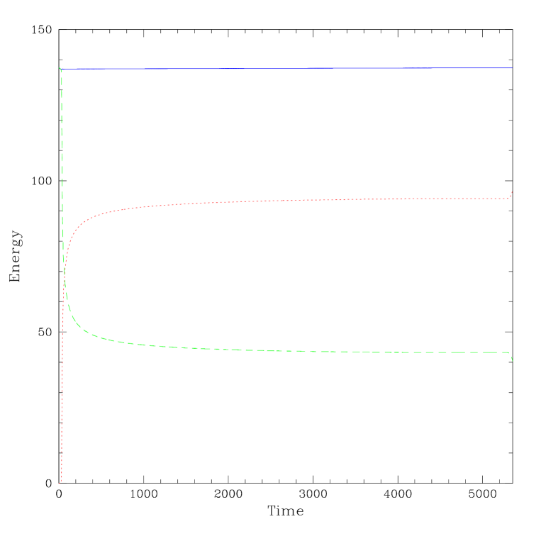
Figure 4.4: Plot of energy contained in oscillon (dashed green lines), energy radiated (dotted red lines), and total energy (solid blue line). The total energy of the system is a constant of motion and is numerically conserved to within a few tenths of a percent (hundredths of a percent if measured from after the initial radiative burst from the collapse). The energy contained within the oscillon drops rapidly during the initial radiative phase and plateaus around $E\approx 43m/\lambda$ during the pseudo-stable regime of the oscillon.

Although monitoring energy conservation is a very important test, it says little about whether there is reflection off of the outer boundary or the $r\approx r_{\rm c}$ region. To check this we compare output from the MIB code to two other types of numerical solutions. The first type of reference solution involves evolution of equation (4.2) in ($\tilde{r}$,$\tilde{t}$) coordinates, but on a grid so large that radiation never reaches the outer boundary (large-grid solutions). These solutions serve as our “ideal” reference solutions (for a given discretization), since we are guaranteed that they are free of contamination from reflections off the outer boundary. The second type of reference solution involves evolution on spatial grid comparable in extent to the MIB grid, but using an outgoing boundary condition (OBC solutions). Since we know these solutions do have error resulting from reflection off of the outer boundary, they demonstrate clearly what can go wrong when the solution becomes contaminated by reflected radiation.

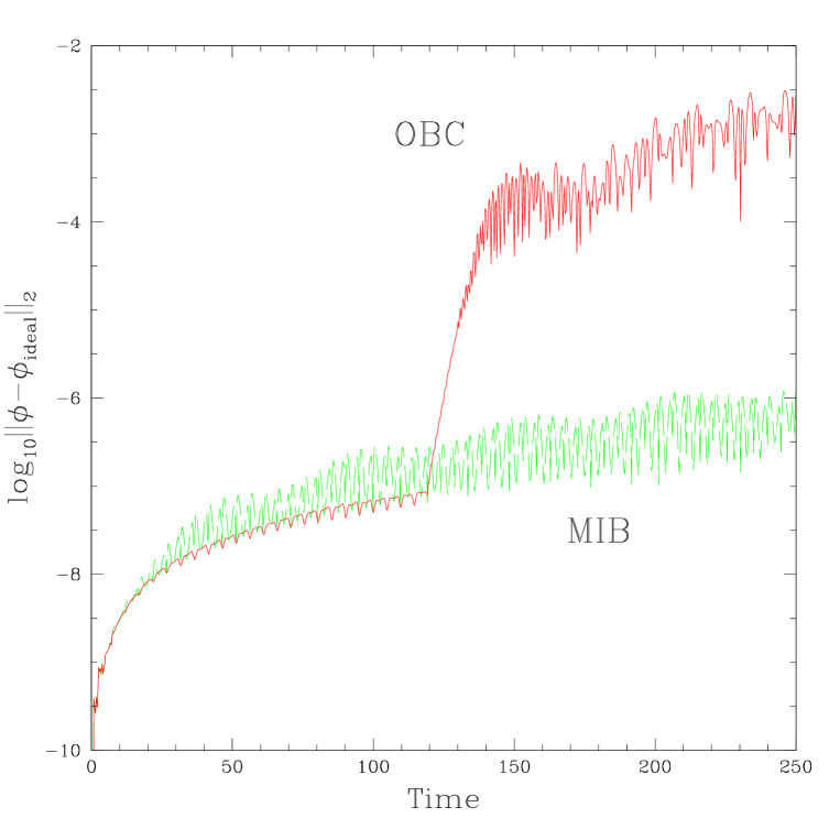
Figure 4.5: Plot comparing the OBC (solid red) and MIB (dashed green) solutions to an “ideal” solution. The OBC solution is obtained using a massless outgoing boundary condition, the MIB solution is obtained by solving the system in spherical MIB coordinates, and the ideal solution is obtained by evolving the solution in standard ($r$,$t$) coordinates on a grid large enough to ensure no reflection off the outer boundary. The error estimates are obtained from the $\ell_{2}$-norm of the difference between the trial solutions (OBC or MIB) and the ideal solution, $||\phi-\phi_{\rm ideal}||_{2}$. Contamination of the OBC solution is observed at two crossing times, $t\approx 120$, where the error estimate increases over three orders of magnitude. The MIB solution error grows slowly and steadily as expected when solving a continuum equation with two different finite difference techniques.

Treating the large-grid solution as ideal, Fig. (4.5) compares typical $\log_{10}||\phi-\phi_{\rm ideal}||_{2}$ for the MIB and OBC solutions. There is a steep increase in the OBC solution error (three orders of magnitude) around $t=125$, which is at roughly two crossing times. This implies that some radiation emitted from the initial collapse reached the outer boundary and reflected back into the region $r<r_{\rm endcap}$. There is no such behavior found in any MIB solutions. Lastly, for a more direct look at the field itself, we can see $\phi(0,t)$ for large-grid (triangles), MIB (solid curves), and OBC (dashed curves) solutions in Fig. (4.6).

Figure 4.6: $\phi(0,t)$ versus time for the large-grid solution (blue triangles), MIB solution (green solid curves), and OBC solution (red dashed curves). The solutions all agree before $2t_{\rm crossing}$, but the OBC solution begins to drift away from the ideal solution after $2t_{\rm crossing}$. The error in the OBC solution is due to radiation that is reflected off of the outer boundary (hence needing two crossing times to return to $r=0$ to contaminate the oscillon). All pictures span the same area, $\Delta\phi=0.075$ by $\Delta t=0.5$.

Initially, both the MIB and OBC solutions agree with the large-grid solution extremely well, while after two crossing times the OBC solution starts to diverge.

Since the MIB solution conserves energy to second order, converges quadratically (in the domain of interest), and is equivalent to the large-grid (again, within second order error), it is an acceptable means of solving equations (4.5,4.6,4.7) while being a great deal more computationally efficient than other previously used techniques. In fact, assuming that dynamical grid methods add more points linearly with time, $N_{r}(t)\propto t$, the total computational work, $W\propto t\,N_{r}(t)$, grows as $t^{2}$. With the MIB method, which uses a static uniform mesh, the computational demand grows linearly with the oscillon lifetime, $W\propto t\,N_{r}$ for $N_{r}$ constant. Thus, particularly for long integration times, there is signifcant cost benefit in using the MIB system instead of a dynamically-growing-grid technique.

4.4 The Resonant Structure of Oscillons
(1D Critical Phenomena I)

Copeland et al. [24], showed quite clearly that oscillons formed for a wide range of initial bubble radii. By collapsing bubbles of many different radii, they even caught a glimpse of resonant structure (which in large part motivated this study) but they did not explore the parameter space in detail. With the efficiency of our new code, we are able to explore much more of the parameter space for a given amount of computational resources than with either large or dynamically growing grids.

Following [23] we use a gaussian profile for initial data where the field at the core and outer boundary values are set to the vacuum values ($\phi_{c}=1$ and $\phi_{o}=-1$ respectively) and the field interpolates between them at a characteristic radius, $r_{0}$:

$$\phi(r,0)=\phi_{o}+\left(\phi_{c}-\phi_{o}\right)\exp\left(-r^{2}/r_{0}^{2}\right).$$ (4.23)

By keeping $\phi_{c}$ and $\phi_{o}$ constant but varying $r_{0}$, we have a one parameter family of initial data to explore. Figure 4.7 shows the behavior of oscillon lifetime as a function of $r_{0}$.

Figure 4.7: Plot of Oscillon lifetime versus initial bubble radius for $2.0\leq r_{0}\leq 5.0$. With the high resolution parameter space survey the 125 resonances become apparent. The survey was conducted at (relatively) coarse resolution to reveal the location of the resonances. Once a resonance was found, it was resolved efficiently first by using a three-point routine that maximizes the lifetime as a function of initial bubble radius, and then by bisecting (to one part in $10^{14}$) on the bifurcate modulation behavior discussed below (and seen in figure 4.9).

We discuss three main findings that are distinct from previous work: the existence of resonances and their time scaling properties, the mode structure of the resonant solutions, and the existence of oscillons outside the region $2\leq r_{0}\leq 5$.

4.4.1 Time Scaling

A new feature is observed in the lifetime profile of collapsing bubbles; figure 4.7 displays the appearance of 125 resonances. These resonances (also seen in Fig. 4.8) become visible only after carefully resolving the parameter space.

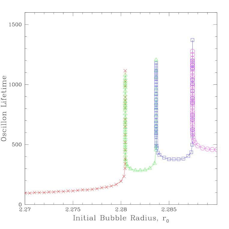
Figure 4.8: Plot of oscillon lifetime versus initial bubble radius for $2.27\leq r_{initial}\leq 2.29$. The three resonances shown occur at $r^{*}_{0}\approx 2.2805$, $r^{*}_{1}\approx 2.2838$, and $r^{*}_{2}\approx 2.2876$. Each resonance separates the parameter space into regions with $n$ and $n+1$ modulations; the red points correspond to oscillons with no modulations, the green points to oscillons with one modulation, the blue to two modulations, and the violet to three modulations.

Upon fine-tuning to one part in $\sim 10^{14}$ we noticed interesting bifurcate behavior about the resonances (figure 4.9, top). The field oscillates with a period $T\approx 4.6$, so the individual oscillations cannot be seen in the plot, but it is the modulation that is of interest here. The top figure shows the envelope of $\phi(0,t)$ on both sides of a resonance (dotted and solid curves). We see that the large period modulation that exists for all typical oscillons disappears late in the lifetime of the oscillon as $r_{0}$ is brought closer to a resonant value (which we define to be $r^{*}_{0}$). On one side of $r^{*}_{0}$ the modulation returns before the oscillon disperses (solid curve), where on the other side, the modulation does not return and the the oscillon just disperses (dotted curve). This behavior does not manifest itself until $r_{0}$ is quite close to $r^{*}_{0}$. So in practice, we used a three point maximization (bracketing interval of $\sim\!0.62$) routine to get $r_{0}$ close to $r^{*}_{0}$ and then we bisected on the bifurcate behavior thereafter (bracketing interval of $0.5$). This is much more efficient than a uniformly sampled parameter space; if the parameter space were sampled uniformly at the finest resolution used in figure 4.7, the survey would contain approximately $3\times 10^{14}$ points, whereas we used only 7605.

Figure 4.9: Top plot shows the envelope of $\phi(0,t)$ for $r^{*}_{0}\!\pm\!\Delta r_{0}$ displaying bifurcate behavior around the $r^{*}_{0}\approx 2.335$ resonance ($\Delta r_{0}\sim 10^{-14}$); the solid red curve is the envelope barely above resonance while green dotted line is the envelope barely below resonance. Bottom plot shows the energy radiated out of the gaussian surface containing the oscillon as a function of time. The increases in the energy radiated are synchronized with the modulation in the field.

Although we can see from Fig. 4.9 that the modulation is directly linked to the resonant solution, it is not obvious why this is so. However, if we look at the relationship between the modulation in the field (top) to the power radiated by the oscillon (bottom), we see that they are clearly synchronized.

This should really be no surprise for one familiar with the 1+1 $KK^{{}^{{}^{{}_{\!\!\!\!\!\!\rule{6.82864pt}{0.7113pt}}}}}$ scattering studied with the same model [10]. Campbell, et al., showed in a study of $KK^{{}^{{}^{{}_{\!\!\!\!\!\!\rule{6.82864pt}{0.7113pt}}}}}$ collisions that after the “prompt radiation” phase (the initial release of radiation upon collision) the remaining radiation emitted is from the decay of what they referred to as “shape” oscillations. The “shape modes” were driven by the contribution to the field “on top” of the $K$ and $K^{{}^{{}^{{}_{\!\!\!\!\!\!\rule{6.82864pt}{0.7113pt}}}}}$ soliton solutions. Since the exact closed-form solution for the ideal non-radiative $KK^{{}^{{}^{{}_{\!\!\!\!\!\!\rule{6.82864pt}{0.7113pt}}}}}$ interaction is not known, initial data are only an approximation and the “leftover” field is responsible for exciting these shape modes. The energy stored in the shape modes slowly decays away as the kink and antikink interact and the solution eventually disperses.

In our case, we believe the large period modulation is signaling the excitation of a similar “shape mode” on top of a periodic, non-radiative, localized, oscillating solution. On either side of a resonance in the $r_{0}$ parameter space, the solution is on the threshold of having one more shape mode oscillation. If this is the case, and we are “tuning in” this unstable shape mode, we might expect to see a scaling law arise.

Figure 4.10: Plot of time scaling, $T$ versus $\ln|r_{0}-r_{0}^{*}|$ for the $r_{0}\approx 2.335$ resonance. The top (blue) line displays the scaling behavior for $r_{0}>r_{0}^{*}$ while the bottom (green) line for $r_{0}<r_{0}^{*}$. The exponents (measured by the slope) are both approximately equal to $\gamma=30$. Although each resonance has a scaling law, the exponents vary from resonance to resonance; a plot of the scaling exponent, $\gamma$, versus the critical initial bubble radius can be seen in figure 4.11.

Figure 4.10 shows a plot of oscillon lifetime versus $\ln|r_{0}-r_{0}^{*}|$ (for the $r_{0}\approx 2.335$ resonance) and we can see quite clearly that there is a scaling law, $T\sim\gamma\ln|r_{0}-r_{0}^{*}|$, for the lifetime of the solution on each side of the resonance. We denote $\gamma_{\rm HI}$ for the scaling exponent on the $r_{0}>r_{0}^{*}$ side, and $\gamma_{\rm LO}$ for the scaling exponent on the $r_{0}<r_{0}^{*}$ side. A plot of both scaling parameters as a function of $r_{0}^{*}$ is seen in Fig. 4.11. We observe that for almost all of the resonances that $\gamma_{\rm HI}\approx\gamma_{\rm LO}$.

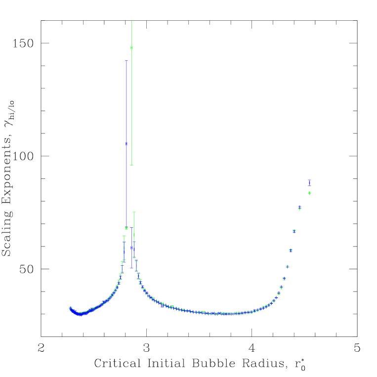
Figure 4.11: Plot of critical exponents for each resonance. There are two values of $\gamma$ for each resonance. The green values are the $\gamma_{\rm hi}$ values measured on the $r_{0}>r_{0}^{*}$ side of the resonance while the blue values are the $\gamma_{\rm lo}$ values measured on the $r_{0}<r_{0}^{*}$ side of the resonance. The uncertainties are estimated from running the entire parameter space surveys at two resolutions and estimating the error, $\Delta\gamma=|\gamma_{(N_{r}=1449)}-\gamma_{(N_{r}=1025)}|$.

4.4.2 Mode Structure

If there does exist a periodic non-radiative solution to equation 4.2, we should be able to construct it by applying an ansatz of the form

$$\phi(r,t)=-1+\phi_{0}(r)+\sum_{n=1}^{\infty}\phi_{n}(r)\cos\left(n\omega t\right)$$ (4.24)

to the equations of motion and solving the resulting system of ordinary differential equations obtained from matching $\cos\left(n\omega t\right)$ terms:

$$\begin{array}[]{rcl}r^{-2}\left(r^{2}\phi_{0}^{\prime}\right)^{\prime}&=&\phi_{0}\left(\phi_{0}-1\right)\left(\phi_{0}-2\right)\\ &&+\frac{3}{2}\left(\phi_{0}-1\right)\sum\limits_{n}\left(\phi_{n}\right)^{2}\\ &&+\frac{1}{4}\sum\limits_{n,p,q}\phi_{n}\phi_{p}\phi_{q}\left(\delta_{n,\pm p\pm q}\right),\end{array}$$ (4.25)

$$\begin{array}[]{rcl}r^{-2}\left(r^{2}\phi_{n}^{\prime}\right)^{\prime}&=&\left(3\left(\phi_{0}-1\right)^{2}-\left(n^{2}\omega^{2}+1\right)\right)\phi_{n}\\ &&+\frac{3}{2}\left(\phi_{0}-1\right)\sum\limits_{p,q}\phi_{p}\phi_{q}\left(\delta_{n,\pm p\pm q}\right)\\ &&+\frac{1}{4}\sum\limits_{m,p,q}\phi_{m}\phi_{n}\phi_{q}\left(\delta_{n,\pm m\pm p\pm q}\right),\end{array}$$ (4.26)

where $\delta_{n,\pm p\pm q}=\left(\delta_{n,+p+q}+\delta_{n,+p-q}+\delta_{n,-p+q}+\delta_{n,-p-q}\right)$, and likewise for $\delta_{n,\pm m\pm p\pm q}$, but with nine terms. Equations 4.25 and 4.26 can also be obtained by inserting ansatz 4.24 into the action and varying with respect to the $\phi_{n}$ [56] (see chapter 6). This set of ODE’s can be solved by “shooting”, where the $\phi_{n}(0)$ are the shooting parameters. Unfortunately, we were unable to construct a method that determined $\omega$ on its own; the best we could do was to solve equations 4.25 and 4.26 for a given $\omega$ that we measured from the dynamic solution. To easily compare the shooting method to the dynamic data, we Fourier decomposed the dynamic data. This was done by taking the solution during the interval of time when the large period modulation disappears ($1200<t<1800$ for the oscillon in Fig. 4.9, for example) and constructing FFTs from the field at each gridpoint, $r_{i}$. The amplitude of each Fourier mode was obtained at each $r_{i}$ from the FFT using a window of 4096 time-slices (bins). These amplitudes were then used to piece together the $\phi_{n}$ (Fig. 4.12).

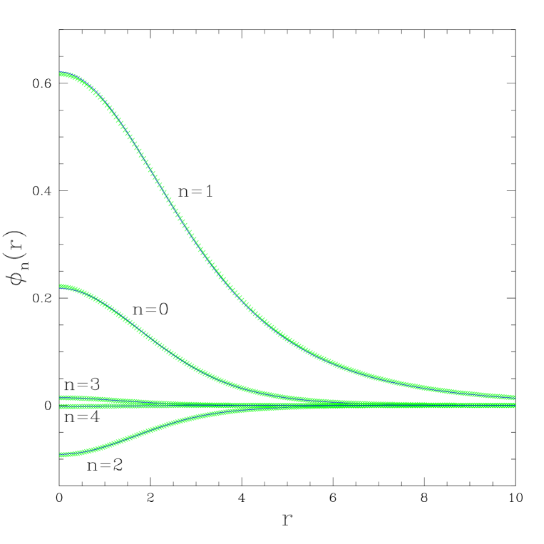
Figure 4.12: Critical solution $\phi_{n}(r)$ (for $n=0,1,2,3,4$) obtained from the Fourier decomposed dynamic data (green x’s) overlayed with $\phi_{n}(r)$ obtained by shooting equations 4.25 and 4.26 (blue solid curves). The dynamic data was Fourier decomposed by forming a time series for each spatial gridpoint, $r_{i}$, while the oscillon entered its non-radiative (no modulation) phase. FFT’s were then constructed for each time series and the amplitude of each mode (the green x’s) was measured.

Keeping only the first five modes, we compare the Fourier decomposed dynamic data with the shooting solution (see Fig. 4.12). The value for $\omega$ was determined from the dynamic solution and the shooting parameters (the $\phi_{n}(0)$) were varied so as to maximize $r_{\rm max}$, the distance before any mode diverged to $\phi\rightarrow\pm\infty$. The correspondence strongly suggests that the resonant solutions (ie. in the limit as $r_{0}\rightarrow r_{0}^{*}$) observed in the dynamic simulations are indeed the periodic non-radiative oscillons obtained from ansatz (4.24)

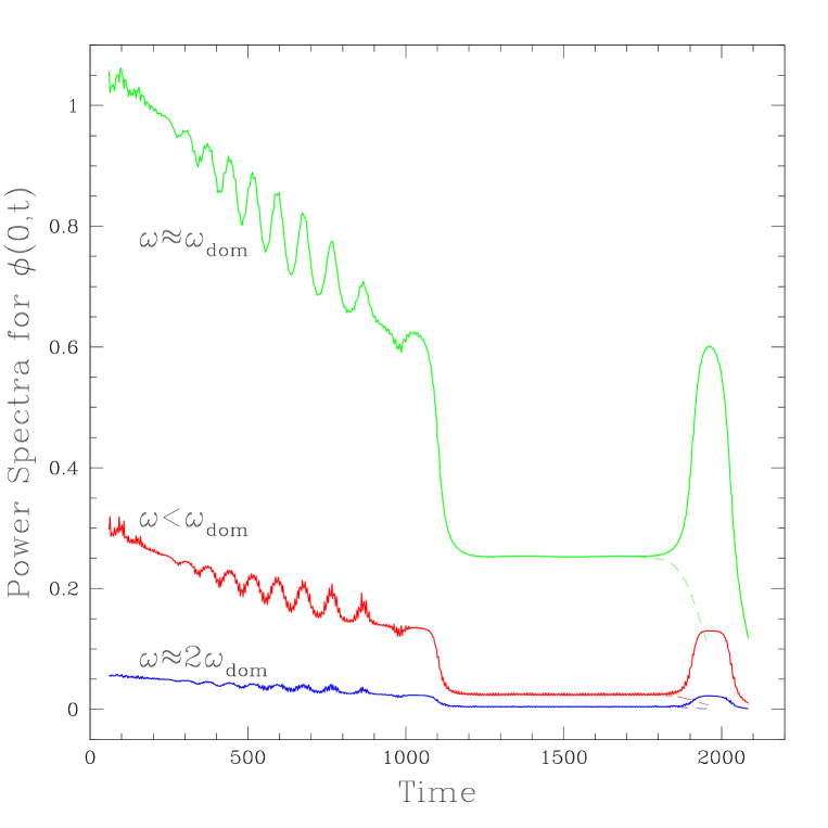
Figure 4.13: Power spectra of the core amplitude, $\phi(0,t)$, for the oscillons barely above and below the $r_{0}\approx 2.335$ resonance. The power measured in each frequency regime slowly diminishes as the oscillon radiates away much of its energy until approximately $t=1100$ where the oscillon enters a non-radiative state and all the components of the power spectrum become constant.

Looking at the three most dominant components of the power spectrum of $\phi(0,t)$, Fig. 4.13, we can see that during the period of no-modulation, the amplitude of each Fourier mode becomes constant. Although the plot is for the core amplitude, $r=0$, this behavior holds for all $r$. This means that a “resonant” oscillon solution latches onto a non-radiative periodic solution as an intermediate attractor. Each resonance, however, does have a different critical solution; figure 4.11 shows distinct critical exponents for each resonance. This is reminiscent of the Type I critical phenomena studied in the massive Einstein-Klein-Gordon (EKG) model, [8], [9], [11], [18], where a family of (apparently) periodic solutions exist on the threshold of black hole formation. The behavior observed here is thus in contradistinction to Type I Einstein-Yang-Mills critical collapse, [15], where the critical solution is found to be static and universal. In any case, instead of existing on the threshold of black hole formation, the critical oscillon solution is an oscillating time-dependent intermediate attractor on the threshold of having one more shape mode oscillation.

4.4.3 (Bounce) Windows to more Oscillons

Lastly, we look at the region of the parameter space beyond $r_{0}\sim 5$. The oscillons explored by Copeland, et al, were restricted to the domain of roughly $2\leq r_{0}\leq 5$. It was even wondered if oscillons could form for larger initial bubble radii. We found that oscillons can form in this region and do so by a rather interesting mechanism.

Again, going back to the 1+1 dimensional $KK^{{}^{{}^{{}_{\!\!\!\!\!\!\rule{6.82864pt}{0.7113pt}}}}}$ scattering of Campbell, et al, it is well known that the kink and antikink often “bounce” many times before either dispersing or falling into an (unstable) bound state. A bounce occurs when the kink and antikink reflect off one another, stop after a short distance, and recollapse. We find that this happens in the (1+1) spherically symmetric case as well, where the unstable bound state is an oscillon. For larger $r_{0}$, instead of the bubble wall remaining within $r\leq 2.5$ (as occurs for $2\leq r_{0}\leq 5$), after reflecting off the origin the bubble wall can travel out to larger r (typically, $3\leq r\leq 6$), stop, and then recollapse, shedding away large amounts of energy in the process;

Figure 4.14: Plot of $\phi(0,t)$ for $r_{0}=7.25$ displaying extremely nonlinear and unpredictable behavior during the “bouncing” phase (for $t<60$), after which the field settles into a typical oscillon evolution. Once in the oscillon regime, the period is approximately $\omega\approx 4.5$, and the first two modulations of the field can be seen (envelope maxima at $t\approx 105$ and $t\approx 200$).

we refer to these regions of parameter space as “bounce windows”. In the recollapse the simulation is effectively starting over with new initial data (albeit a different shape) but with much less energy (smaller $r_{0}$). In Fig. 4.15 we see a lifetime profile and its resonances for a typical bounce window.

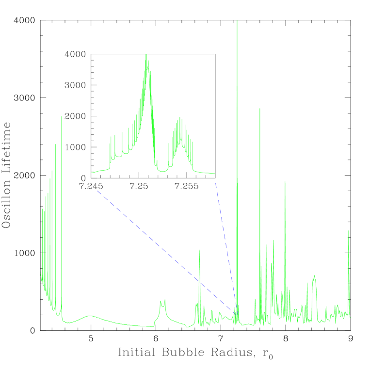
Figure 4.15: Plot of oscillon lifetime versus initial radius of bubble for $4.22\leq r_{0}\leq 9$. Although there seem to be no oscillons within $4.6\leq r_{0}\leq 6$, it is clear that oscillons do exist for higher initial bubble radii. Furthermore, within these “windows” of parameter space that support oscillon formation, there also exist resonances similar to those observed throughout the $2\leq r_{0}\leq 4.6$ region (see inset to observe resonances within $7.245\leq r_{0}\leq 7.257$).

4.5 The Klein-Gordon Equation in MIB Coordinates with ADWP (1D Critical Phenomena II)

This chapter concludes with time evolution of spherically symmetric bubbles in the context of a slightly different action than the one introduced in section 4.1. The action used is the same as equation (4.1),

$$S[\phi]=\int d^{4}x\sqrt{|g|}\left(-\frac{1}{2}g^{\mu\nu}\nabla_{\mu}\phi\nabla_{\nu}\phi-V(\phi)\right),$$ (4.27)

except with an asymmetric potential, $\displaystyle{V(\phi)\equiv V_{A}(\phi)=\frac{1}{4}\phi^{2}\left(\phi^{2}-4\left(1+\delta\right)\phi+4\right)}$ where again $\phi\equiv\phi(r,t)$, and $\delta$ is a measure of the asymmetry of the potential. When $\delta=0$, $\displaystyle{V_{A}(\phi)}$ has the same shape as the SDWP potential of Chapter 4, but is shifted so that the vacuum states are at $\phi=0$ and $\phi=2$. With $\delta\neq 0$, the false and true vacuum states are $\phi_{F}=0$ and $\displaystyle{\phi_{T}=\frac{3}{2}\left(1+\delta\right)+\frac{1}{2}\sqrt{1+18\delta+\delta^{2}}}$, respectively.

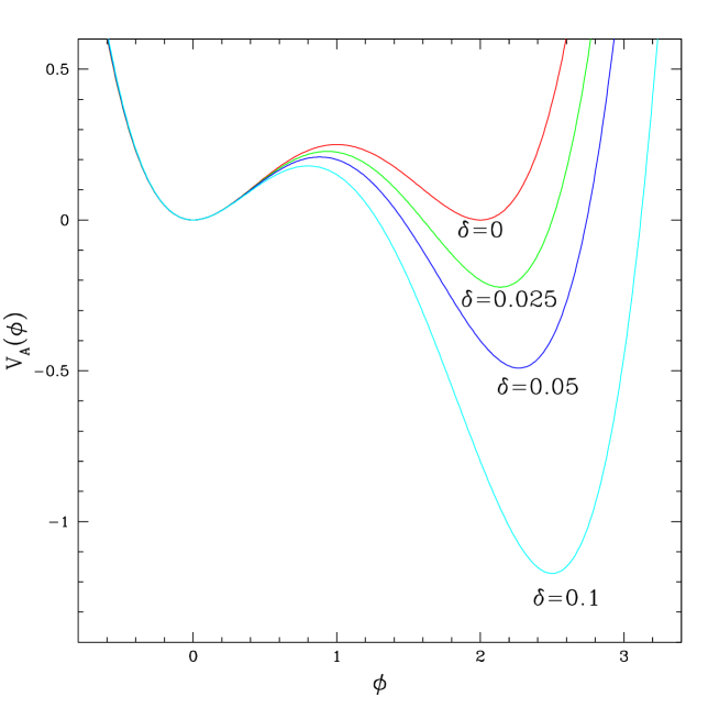
Figure 4.16: Asymmetric double well potential $\displaystyle{V_{A}(\phi)=\frac{1}{4}\phi^{2}\left(\phi^{2}-4\left(1+\delta\right)\phi+4\right)}$ for various values of asymmetry parameter, $\delta$. Minima are clearly not degenerate for $\delta\neq 0$ and are at $\phi_{F}=0$ and $\displaystyle{\phi_{T}=\frac{3}{2}\left(1+\delta\right)+\frac{1}{2}\sqrt{1+18\delta+\delta^{2}}}$ (the false vacuum and true vacuum states, respectively).

The spherically symmetric MIB code is (trivially) modified by replacing the potential terms in the finite difference equations with the new potential, leaving $\delta$ as a run-time parameter. Instead of performing extensive parameter space surveys with this potential like in section (4.4), a different type of phenomena is explored. With the introduction of the asymmetric potential which has non-degenerate vacuum states, the threshold of expanding bubble formation can be examined. As discussed in section (2.1), the initial bubble radius can be used to define a one-parameter family of initial data that transitions from bubble collapse (and eventual dispersal) to expanding bubble formation. As one familiar with critical phenomena might expect, there exists a time scaling law for the lifetime of the bubble lying on this threshold. The time scaling exponent is observed to be, $\gamma\simeq 2.1$, where $T\propto-\gamma\ln|\sigma-\sigma^{*}|$.

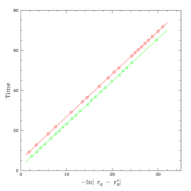
Figure 4.17: Plot of oscillon lifetime as a function of $-\ln|r_{0}-r_{0}^{*}|$ for the collapse (or expansion) of static bubble initial data using the ADWP. The lifetimes on the collapsing side of criticality are represented by green triangles, while the lifetimes on the expanding side of criticality are represented by red triangles. There is a single time scaling law with scaling exponent (slope) $\gamma\approx 2.1$.

Chapter 5 Axi-Symmetric Oscillon Dynamics

This chapter discusses our investigations of the non-linear Klein-Gordon model in axisymmetry. The equation of motion is written in 2-D MIB coordinates and a finite difference version of the equations is presented. The convergence properties of the code which solves the difference equations are shown, and evidence to support the validity of the MIB system as an effective absorbing outer-boundary is presented. A simple numerical technique is presented that allows for the arbitrary Lorentz boosting of spherically symmetric data. Finally, the code is used to collide two oscillons and a time-scaling phenomenon analogous to that seen in chapter 4.5 is observed.

5.1 The Klein-Gordon Equation in Axi-Symmetric MIB Coordinates

This section discusses the implementation of 2-D MIB coordinates in the solution of the nonlinear Klein-Gordon model with an asymmetric double-well (ADWP) potential. The model studied is the same ADWP model just used to study the threshold of expanding bubble formation in the previous chapter. The resultant PDE we must solve is still simply the Klein-Gordon equation

$$\frac{1}{\sqrt{|g|}}\partial_{\mu}\left(\sqrt{|g|}g^{\mu\nu}\partial_{\nu}\phi\right)=\phi\left(\phi^{2}-3\left(1-\delta\right)+2\right)$$ (5.1)

but now with $\phi\equiv\phi(R,z,t)$. Defining

$$\displaystyle{\Pi(R,z,t)} \equiv \displaystyle{ab\left(\dot{\phi}-\beta^{R}\Phi_{R}-\beta^{z}\Phi_{z}\right)},$$ (5.2)

$$\displaystyle{\Phi_{R}(R,z,t)} \equiv \displaystyle{\partial_{R}\phi,}$$ (5.3)

$$\displaystyle{\Phi_{z}(R,z,t)} \equiv \displaystyle{\partial_{z}\phi,}$$ (5.4)

we have

$$\dot{\Pi} = 2a\frac{\partial}{\partial\left(\tilde{R}^{2}\right)}\left[\tilde{R}\left(\beta^{R}\Pi+\frac{b}{a}\Phi_{R}\right)\right]+\frac{\partial}{\partial z}\left(\beta^{z}\Pi+\frac{a}{b}\Phi_{z}\right)$$ (5.5)

$$-\frac{\dot{\tilde{R}}}{\tilde{R}}\Pi-ab\frac{\partial V}{\partial\phi}$$

$$\dot{\Phi}_{R} = \frac{\partial}{\partial R}\left(\frac{1}{ab}\Pi+\beta^{R}\Phi_{R}+\beta^{z}\Phi_{z}\right)$$ (5.6)

$$\dot{\Phi}_{z} = \frac{\partial}{\partial z}\left(\frac{1}{ab}\Pi+\beta^{R}\Phi_{R}+\beta^{z}\Phi_{z}\right)$$ (5.7)

$$\dot{\phi} = \frac{1}{ab}\Pi+\beta^{R}\Phi_{R}+\beta^{z}\Phi_{z},$$ (5.8)

for $a$, $b$, $\beta^{R}$, $\beta^{z}$, $\alpha$, and $\tilde{R}$ functions of $R$, $z$, and $t$, as defined in equations (3.27). As with the spherically symmetric case, these equations are similar in form to the Klein-Gordon equation coupled to gravity, except that, again, the “geometric variables” are known functions of our coordinates.

5.2 Finite Difference Equations

Equations (5.5), (5.6), (5.7), and (5.8) are solved using two-level second order (in both space and time) finite difference approximations on a static uniform mesh with $N_{R}$ by $N_{z}$ grid points in the $R$ and $z$ directions, respectively. The scale of discretization is set by $\Delta R$, $\Delta z$, and $\Delta t=\lambda\min(\Delta R,\Delta z)$. The field variables were first updated without dissipation everywhere (yielding the $\hat{}$ variables), and then dissipation was added were possible (yielding the $\tilde{}$ and final quantities). Using the difference operators from Table 3.2, $\partial_{R}\tilde{R}=a$, and $\partial_{R}=nR^{n-1}\partial_{R^{n}}$, the interior ($2\leq i\leq N_{R}-1$, $2\leq j\leq N_{z}-1$) difference equations are:
$\displaystyle\Delta_{t}\hat{\Pi}^{n}_{i,j}$ $\displaystyle=$ $\displaystyle 2\mu^{ave}_{t}\left[a^{n}_{i,j}\Delta_{\tilde{R}^{2}}\left(\tilde{R}\left(\displaystyle{\beta^{R}\Pi+\frac{b}{a}\Phi_{R}}\right)\right)+\Delta_{z}\left(\displaystyle{\beta^{z}\Pi+\frac{a}{b}\Phi_{z}}\right)\right]^{n}_{i,j}$ (5.9) $\displaystyle-\displaystyle{\mu^{ave}_{t}\left(\frac{\dot{\tilde{R}}}{\tilde{R}}\Pi-ab\phi\left(\phi^{2}-3\left(1+\delta\right)\phi+2\right)\right)^{n}_{i,j}},$ $\displaystyle\Delta_{t}{\left(\hat{\Phi}_{R}\right)}^{n}_{i,j}$ $\displaystyle=$ $\displaystyle\mu^{ave}_{t}\Delta_{R}\left(\frac{1}{ab}\Pi+\beta^{R}\Phi_{R}+\beta^{z}\Phi^{z}\right)^{n}_{i,j},$ (5.10) $\displaystyle\Delta_{t}{\left(\hat{\Phi}_{z}\right)}^{n}_{i,j}$ $\displaystyle=$ $\displaystyle\mu^{ave}_{t}\Delta_{z}\left(\frac{1}{ab}\Pi+\beta^{R}\Phi_{R}+\beta^{z}\Phi^{z}\right)^{n}_{i,j},$ (5.11) $\displaystyle\Delta_{t}\hat{\phi}^{n}_{i,j}$ $\displaystyle=$ $\displaystyle\mu^{ave}_{t}\left(\frac{1}{ab}\Pi+\beta^{R}\Phi_{R}+\beta^{z}\Phi^{z}\right)^{n}_{i,j}.$ (5.12) For the inner $R=0$ boundary ($i=1$, $2\leq j\leq N_{z}-1$), the conditions for regularity at the origin are applied for $\Phi_{R}$ and $\Pi$ (analogous to equations (4.15) and (4.16) for spherical symmetry):

$$\mu^{ave}_{t}\left[\Delta^{f}_{R}\hat{\Pi}-\frac{a^{\prime}}{a}\hat{\Pi}\right]^{n}_{i,j} = 0$$ (5.13)

$$\left(\hat{\Phi_{R}}\right)^{n+1}_{i,j} = 0$$ (5.14)

while evolving $\hat{\Phi}_{z}$ and $\hat{\phi}$ as in the interior of the grid

$$\Delta_{t}{\left(\hat{\Phi}_{z}\right)}^{n}_{i,j}-\mu^{ave}_{t}\Delta_{z}\left(\frac{1}{ab}\Pi+\beta^{R}\Phi_{R}+\beta^{z}\Phi^{z}\right)^{n}_{i,j} = 0$$ (5.15)

$$\Delta_{t}\hat{\phi}^{n}_{i,j}-\mu^{ave}_{t}\left(\frac{1}{ab}\Pi+\beta^{R}\Phi_{R}+\beta^{z}\Phi^{z}\right)^{n}_{i,j} = 0.$$ (5.16)

For the outer boundaries, as with the spherically symmetric case, the equations used make very little difference since the physical position ($\tilde{R}$,$\tilde{z}$) corresponding to the outermost gridpoint is moving out at nearly the speed of light. Therefore none of the outgoing field actually reaches the outer ($R$,$z$) boundary. Nevertheless, the typical massless scalar field outgoing boundary condition is imposed (on three edges and four corners):

$$\Delta_{t}\hat{\Pi}^{n}_{i,j} = \mu^{ave}_{t}\left[\displaystyle{\frac{R\Delta^{b}_{R}\Pi+z\Delta_{z}\Pi+\Pi}{\sqrt{R^{2}+z^{2}}}}\right]^{n}_{i,j}$$ (5.17)

$$\Delta_{t}\left(\hat{\Phi}_{R}\right)^{n}_{i,j} = \mu^{ave}_{t}\left[\displaystyle{\frac{R\Delta^{b}_{R}\left(\Phi_{R}\right)+z\Delta_{z}\left(\Phi_{R}\right)+\left(\Phi_{R}\right)}{\sqrt{R^{2}+z^{2}}}}\right]^{n}_{i,j}$$ (5.18)

$$\Delta_{t}\left(\hat{\Phi}_{z}\right)^{n}_{i,j} = \mu^{ave}_{t}\left[\displaystyle{\frac{R\Delta^{b}_{R}\left(\Phi_{z}\right)+z\Delta_{z}\left(\Phi_{z}\right)+\left(\Phi_{z}\right)}{\sqrt{R^{2}+z^{2}}}}\right]^{n}_{i,j}$$ (5.19)

$$\Delta_{t}\hat{\phi}^{n}_{i,j} = \mu^{ave}_{t}\left[\frac{1}{ab}\Pi+\beta^{R}\Phi_{R}+\beta^{z}\Phi^{z}\right]^{n}_{i,j}$$ (5.20)

for $i=N_{R}$, $2\leq j\leq N_{z}-1$,

$$\Delta_{t}\hat{\Pi}^{n}_{i,j} = \mu^{ave}_{t}\left[\displaystyle{\frac{R\Delta_{R}\Pi+z\Delta^{f}_{z}\Pi+\Pi}{\sqrt{R^{2}+z^{2}}}}\right]^{n}_{i,j}$$ (5.21)

$$\Delta_{t}\left(\hat{\Phi}_{R}\right)^{n}_{i,j} = \mu^{ave}_{t}\left[\displaystyle{\frac{R\Delta_{R}\left(\Phi_{R}\right)+z\Delta^{f}_{z}\left(\Phi_{R}\right)+\left(\Phi_{R}\right)}{\sqrt{R^{2}+z^{2}}}}\right]^{n}_{i,j}$$ (5.22)

$$\Delta_{t}\left(\hat{\Phi}_{z}\right)^{n}_{i,j} = \mu^{ave}_{t}\left[\displaystyle{\frac{R\Delta_{R}\left(\Phi_{z}\right)+z\Delta^{f}_{z}\left(\Phi_{z}\right)+\left(\Phi_{z}\right)}{\sqrt{R^{2}+z^{2}}}}\right]^{n}_{i,j}$$ (5.23)

$$\Delta_{t}\hat{\phi}^{n}_{i,j} = \mu^{ave}_{t}\left[\frac{1}{ab}\Pi+\beta^{R}\Phi_{R}+\beta^{z}\Phi^{z}\right]^{n}_{i,j}$$ (5.24)

for $j=1$, $1\leq i\leq N_{R}$,

$$\Delta_{t}\hat{\Pi}^{n}_{i,j} = \mu^{ave}_{t}\left[\displaystyle{\frac{R\Delta_{R}\Pi+z\Delta^{b}_{z}\Pi+\Pi}{\sqrt{R^{2}+z^{2}}}}\right]^{n}_{i,j}$$ (5.25)

$$\Delta_{t}\left(\hat{\Phi}_{R}\right)^{n}_{i,j} = \mu^{ave}_{t}\left[\displaystyle{\frac{R\Delta_{R}\left(\Phi_{R}\right)+z\Delta^{b}_{z}\left(\Phi_{R}\right)+\left(\Phi_{R}\right)}{\sqrt{R^{2}+z^{2}}}}\right]^{n}_{i,j}$$ (5.26)

$$\Delta_{t}\left(\hat{\Phi}_{z}\right)^{n}_{i,j} = \mu^{ave}_{t}\left[\displaystyle{\frac{R\Delta_{R}\left(\Phi_{z}\right)+z\Delta^{b}_{z}\left(\Phi_{z}\right)+\left(\Phi_{z}\right)}{\sqrt{R^{2}+z^{2}}}}\right]^{n}_{i,j}$$ (5.27)

$$\Delta_{t}\hat{\phi}^{n}_{i,j} = \mu^{ave}_{t}\left[\frac{1}{ab}\Pi+\beta^{R}\Phi_{R}+\beta^{z}\Phi^{z}\right]^{n}_{i,j}$$ (5.28)

for $j={\rm R_{z}}$, $1\leq i\leq N_{R}$,

$$\Delta_{t}\hat{\Pi}^{n}_{i,j} = \mu^{ave}_{t}\left[\displaystyle{\frac{R\Delta^{f}_{R}\Pi+z\Delta^{f}_{z}\Pi+\Pi}{\sqrt{R^{2}+z^{2}}}}\right]^{n}_{i,j}$$ (5.29)

$$\Delta_{t}\left(\hat{\Phi}_{R}\right)^{n}_{i,j} = \mu^{ave}_{t}\left[\displaystyle{\frac{R\Delta^{f}_{R}\left(\Phi_{R}\right)+z\Delta^{f}_{z}\left(\Phi_{R}\right)+\left(\Phi_{R}\right)}{\sqrt{R^{2}+z^{2}}}}\right]^{n}_{i,j}$$ (5.30)

$$\Delta_{t}\left(\hat{\Phi}_{z}\right)^{n}_{i,j} = \mu^{ave}_{t}\left[\displaystyle{\frac{R\Delta^{f}_{R}\left(\Phi_{z}\right)+z\Delta^{f}_{z}\left(\Phi_{z}\right)+\left(\Phi_{z}\right)}{\sqrt{R^{2}+z^{2}}}}\right]^{n}_{i,j}$$ (5.31)

$$\Delta_{t}\hat{\phi}^{n}_{i,j} = \mu^{ave}_{t}\left[\frac{1}{ab}\Pi+\beta^{R}\Phi_{R}+\beta^{z}\Phi^{z}\right]^{n}_{i,j}$$ (5.32)

for $i=1$, $j=1$,

$$\Delta_{t}\hat{\Pi}^{n}_{i,j} = \mu^{ave}_{t}\left[\displaystyle{\frac{R\Delta^{b}_{R}\Pi+z\Delta^{f}_{z}\Pi+\Pi}{\sqrt{R^{2}+z^{2}}}}\right]^{n}_{i,j}$$ (5.33)

$$\Delta_{t}\left(\hat{\Phi}_{R}\right)^{n}_{i,j} = \mu^{ave}_{t}\left[\displaystyle{\frac{R\Delta^{b}_{R}\left(\Phi_{R}\right)+z\Delta^{f}_{z}\left(\Phi_{R}\right)+\left(\Phi_{R}\right)}{\sqrt{R^{2}+z^{2}}}}\right]^{n}_{i,j}$$ (5.34)

$$\Delta_{t}\left(\hat{\Phi}_{z}\right)^{n}_{i,j} = \mu^{ave}_{t}\left[\displaystyle{\frac{R\Delta^{b}_{R}\left(\Phi_{z}\right)+z\Delta^{f}_{z}\left(\Phi_{z}\right)+\left(\Phi_{z}\right)}{\sqrt{R^{2}+z^{2}}}}\right]^{n}_{i,j}$$ (5.35)

$$\Delta_{t}\hat{\phi}^{n}_{i,j} = \mu^{ave}_{t}\left[\frac{1}{ab}\Pi+\beta^{R}\Phi_{R}+\beta^{z}\Phi^{z}\right]^{n}_{i,j}$$ (5.36)

for $i=N_{R}$, $j=1$,

$$\Delta_{t}\hat{\Pi}^{n}_{i,j} = \mu^{ave}_{t}\left[\displaystyle{\frac{R\Delta^{f}_{R}\Pi+z\Delta^{b}_{z}\Pi+\Pi}{\sqrt{R^{2}+z^{2}}}}\right]^{n}_{i,j}$$ (5.37)

$$\Delta_{t}\left(\hat{\Phi}_{R}\right)^{n}_{i,j} = \mu^{ave}_{t}\left[\displaystyle{\frac{R\Delta^{f}_{R}\left(\Phi_{R}\right)+z\Delta^{b}_{z}\left(\Phi_{R}\right)+\left(\Phi_{R}\right)}{\sqrt{R^{2}+z^{2}}}}\right]^{n}_{i,j}$$ (5.38)

$$\Delta_{t}\left(\hat{\Phi}_{z}\right)^{n}_{i,j} = \mu^{ave}_{t}\left[\displaystyle{\frac{R\Delta^{f}_{R}\left(\Phi_{z}\right)+z\Delta^{b}_{z}\left(\Phi_{z}\right)+\left(\Phi_{z}\right)}{\sqrt{R^{2}+z^{2}}}}\right]^{n}_{i,j}$$ (5.39)

$$\Delta_{t}\hat{\phi}^{n}_{i,j} = \mu^{ave}_{t}\left[\frac{1}{ab}\Pi+\beta^{R}\Phi_{R}+\beta^{z}\Phi^{z}\right]^{n}_{i,j}$$ (5.40)

for $i=1$, $j=N_{z}$, and finally

$$\Delta_{t}\hat{\Pi}^{n}_{i,j} = \mu^{ave}_{t}\left[\displaystyle{\frac{R\Delta^{b}_{R}\Pi+z\Delta^{b}_{z}\Pi+\Pi}{\sqrt{R^{2}+z^{2}}}}\right]^{n}_{i,j}$$ (5.41)

$$\Delta_{t}\left(\hat{\Phi}_{R}\right)^{n}_{i,j} = \mu^{ave}_{t}\left[\displaystyle{\frac{R\Delta^{b}_{R}\left(\Phi_{R}\right)+z\Delta^{b}_{z}\left(\Phi_{R}\right)+\left(\Phi_{R}\right)}{\sqrt{R^{2}+z^{2}}}}\right]^{n}_{i,j}$$ (5.42)

$$\Delta_{t}\left(\hat{\Phi}_{z}\right)^{n}_{i,j} = \mu^{ave}_{t}\left[\displaystyle{\frac{R\Delta^{b}_{R}\left(\Phi_{z}\right)+z\Delta^{b}_{z}\left(\Phi_{z}\right)+\left(\Phi_{z}\right)}{\sqrt{R^{2}+z^{2}}}}\right]^{n}_{i,j}$$ (5.43)

$$\Delta_{t}\hat{\phi}^{n}_{i,j} = \mu^{ave}_{t}\left[\frac{1}{ab}\Pi+\beta^{R}\Phi_{R}+\beta^{z}\Phi^{z}\right]^{n}_{i,j}$$ (5.44)

for $i=N_{R}$, $j=N_{z}$. This condition is derived by transforming the spherically symmetric out-going boundary condition to axisymmetric coordinates. This is a reasonable approach to take since at large distances away from the collision, the emitted wave-fronts do becomes spherical.

After each update using the evolution equations, dissipation is added independently in each spatial direction wherever the action of the appropriate dissipation operator is well-defined. Specifically, the fields are updated a second time (second updated quantities denoted by $\tilde{}$ ) using $\mu^{\rm diss}_{R}$ according to

$$\tilde{\Pi}^{n+1}_{i,j} = \hat{\Pi}^{n+1}_{i,j}+\mu^{\rm diss}_{R}\hat{\Pi}^{n}_{i,j}$$ (5.45)

$$\left(\tilde{\Phi}_{R}\right)^{n+1}_{i,j} = \left(\hat{\Phi}_{R}\right)^{n+1}_{i,j}+\mu^{\rm diss}_{R}\left(\hat{\Phi_{R}}\right)^{n}_{i,j}$$ (5.46)

$$\left(\tilde{\Phi}_{z}\right)^{n+1}_{i,j} = \left(\hat{\Phi}_{z}\right)^{n+1}_{i,j}+\mu^{\rm diss}_{R}\left(\hat{\Phi_{z}}\right)^{n}_{i,j}$$ (5.47)

$$\tilde{\phi}^{n+1}_{i,j} = \hat{\phi}^{n+1}_{i,j}+\mu^{\rm diss}_{R}\hat{\phi}^{n}_{i,j}$$ (5.48)

where $3\leq i\leq N_{r}-2$ and $1\leq j\leq N_{z}$. Then the fields are updated a third time (third updated quantities have no accent) using $\mu^{\rm diss}_{z}$ according to

$$\Pi^{n+1}_{i,j} = \tilde{\Pi}^{n+1}_{i,j}+\mu^{\rm diss}_{z}\tilde{\Pi}^{n}_{i,j}$$ (5.49)

$$\left(\Phi_{R}\right)^{n+1}_{i,j} = \left(\tilde{\Phi}_{R}\right)^{n+1}_{i,j}+\mu^{\rm diss}_{z}\left(\tilde{\Phi}_{R}\right)^{n}_{i,j}$$ (5.50)

$$\left(\Phi_{z}\right)^{n+1}_{i,j} = \tilde{\left(\tilde{\Phi}_{z}\right)}^{n+1}_{i,j}+\mu^{\rm diss}_{z}\left(\tilde{\Phi}_{z}\right)^{n}_{i,j}$$ (5.51)

$$\phi^{n+1}_{i,j} = \tilde{\phi}^{n+1}_{i,j}+\mu^{\rm diss}_{R}\tilde{\phi}^{n}_{i,j}$$ (5.52)

where $3\leq j\leq N_{z}-2$ and $1\leq i\leq N_{r}$. The three update steps comprise one iteration. Typically, the whole process is repeated until the solutions at the ($n+1$) time step converge to one part in $10^{10}$.

5.3 Testing the 2-D code

Although the 1-D MIB code worked very well, it was not obvious a priori that the same success would be achievable in a 2-D axisymmetric code. However, we find that the code is stable and passes all the desired tests; it is second-order convergent in general, it conserves energy to second-order in particular, and outgoing radiation is absorbed without reflection, so that there is no noticeable contamination of the interior solution (at least at the level of accuracy at which we work).

Again, since equation (5.1) is a flatspace wave equation, obtaining a globally conserved energy is straightforward. The spacetime admits a timelike Killing vector, $t^{\nu}$, and therefore has a conserved current, $J_{\mu}=t^{\nu}T_{\mu\nu}$. A gaussian surface is constructed between two spacelike hypersurfaces within a cylindrical spatial domain $0\leq R\leq R_{\rm endcap}$, $-z_{\rm endcap}\leq z\leq z_{\rm endcap}$, with normals $n_{\mu}=(\pm 1,0,0,0)$ (the timelike normal to the hypersurfaces), $n_{R}^{\mu}=(0,a^{-1},0,0)$ (the normal to the side of the spatial gaussian cylinder), and $n_{z}^{\mu}=(0,0,0,\pm b^{-1})$ (the normals to the top and bottom of the spatial gaussian cylinder). To obtain the conserved energy at a time, $t_{f}$, the energy contained within the bubble,

$$E_{\rm bubble}(t)=2\pi\int\limits_{\!\!0}^{\ \ \ R_{endcap}}\int\limits_{-z_{\rm endcap}}^{\ \ \ z_{\rm endcap}}R\left(\frac{\Pi^{2}}{2a^{2}b^{2}}+\frac{\Phi_{R}^{2}}{2a^{2}}+\frac{\Phi_{z}^{2}}{2b^{2}}+V\left(\phi\right)\right)dr\ dz,$$ (5.53)

(where the integrand is evaluated at time $t$) is added to the total radiated energy, $E_{\rm rad}(t)=E^{R_{\rm endcap}}_{\rm rad}+E^{Z^{+}_{\rm endcap}}_{\rm rad}+E^{Z^{-}_{\rm endcap}}_{\rm rad}$, where

$$E^{R_{\rm endcap}}_{\rm rad}(t)=2\pi R\int\limits_{\!\!0}^{\ t}\int\limits_{-z_{\rm endcap}}^{\ \ \ z_{\rm endcap}}\left(\frac{\Pi\Phi_{R}}{ab}\right)dz\ dt^{\prime}$$ (5.54)

(where the integrand is evaluated at $R=R_{\rm endcap}$) and

$$E^{Z^{\pm}_{\rm endcap}}_{\rm rad}(t)=2\pi\int\limits_{\!\!0}^{\ t}\int\limits_{\!\!0}^{\ \ \ R_{\rm endcap}}R\left(\frac{\Pi\Phi_{z}}{ab}\right)dR\ dt^{\prime}$$ (5.55)

(where the integrand is evaluated at $z=\pm z_{\rm endcap}$). The sum, $E_{\rm total}=E_{\rm bubble}+E_{\rm rad}$, remains conserved to within a percent at $201\times 401$ gridpoints (see figure 5.1 for energy as a function of time, see figure 5.2 to see more clearly the energy being conserved as per second order convergence).

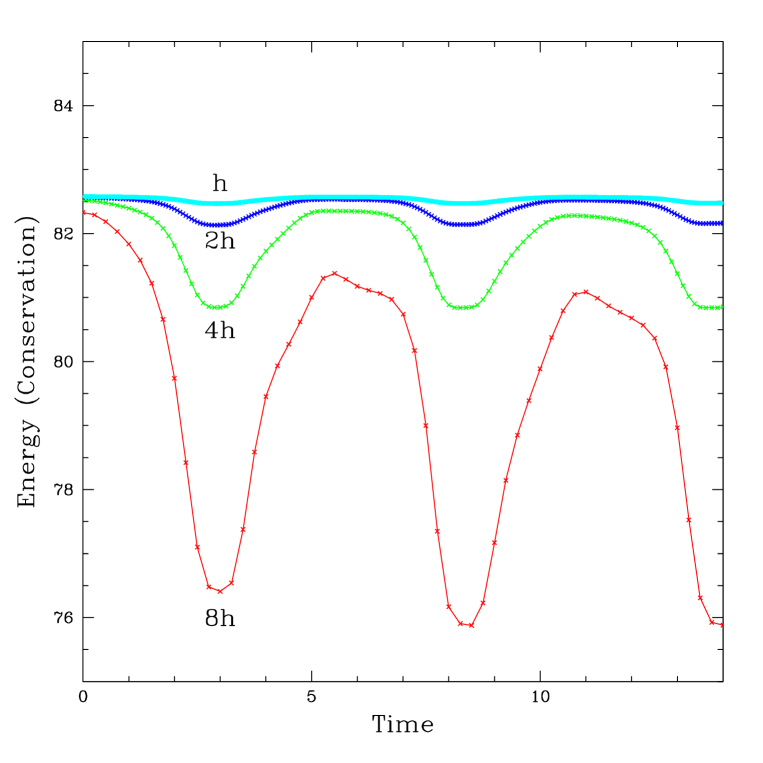
Figure 5.1: Energy conservation of 2D code at four discretizations, $41\times 81$, $81\times 161$, $161\times 321$, and $321\times 641$ gridpoints (8h, 4h, 2h, and h, respectively). The code conserves energy approximately to one part in 13, 50, 200, and 800, for levels 8h, 4h, 2h, and h, respectively, thus displaying energy conservation consistent with a second-order convergent code.

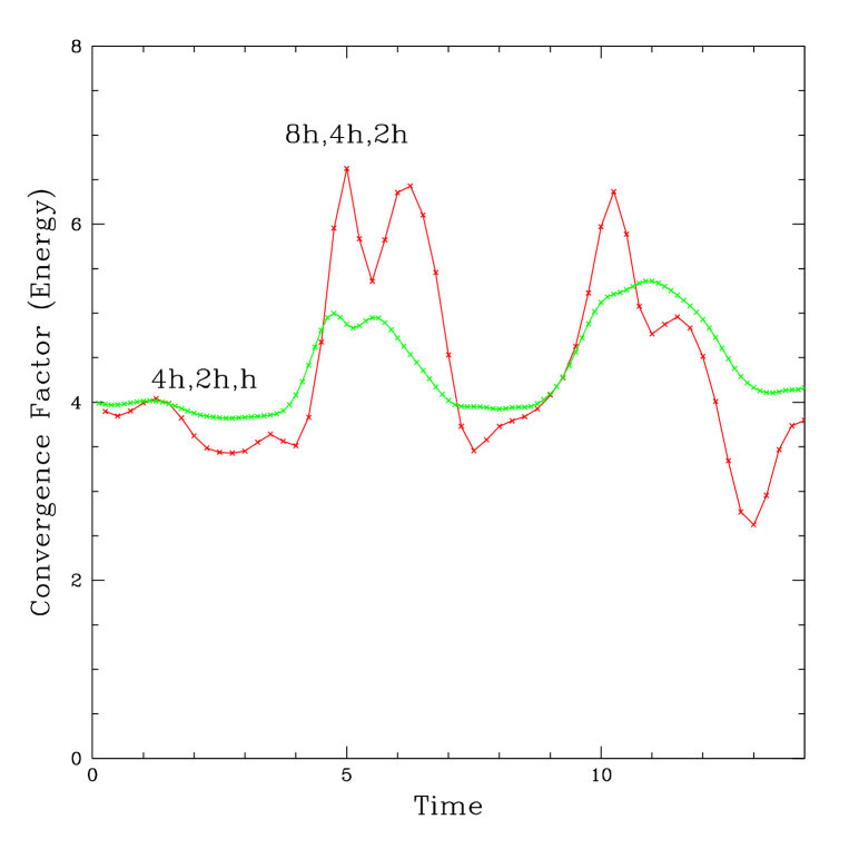
Figure 5.2: Convergence factors, $\left(E_{4h}-E_{2h}\right)/\left(E_{2h}-E_{h}\right)$ in red and $\left(E_{8h}-E_{4h}\right)/\left(E_{4h}-E_{2h}\right)$ in green, for the conserved energy. As with the convergence tests in chapter 4 (figure 4.3, in particular) a convergence factor of four indicates second-order convergence. The code clearly conserves energy to second order.

In addition to conserving energy (to second order), the code displays second order convergence in all the evolved field variables (see figure 5.3).

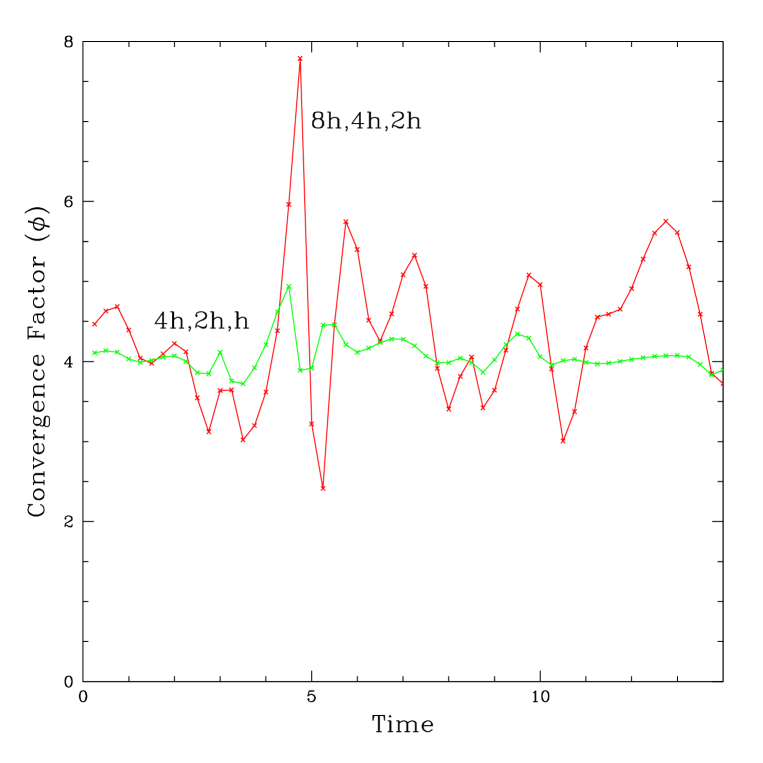
Figure 5.3: Convergence of 2D code for the field $\phi$ at four discretizations, $41\times 81$, $81\times 161$, $161\times 321$, and $321\times 641$ gridpoints (8$h$, 4$h$, 2$h$, and $h$, respectively). The convergence factors for levels 8$h$, 4$h$, and 2$h$ and levels 4$h$, 2$h$, and $h$ are shown in red and green, respectively. The value of roughly four observed for each convergence factor indicates that the code is indeed second-order.

However, convergent energy conservation and convergent field variables do not imply that the MIB system is absorbing the outgoing radiation properly.

To verify that there is no significant reflected radiation off the outer boundary that contaminates the solution (exactly following the methods described in section 4.3) the MIB solution is compared to an ideal large-grid solution by taking the $\ell_{2}$-norm of the difference at every point,

$$||A||_{F}=\left(\frac{1}{MN}\sum_{ij}|a_{ij}|^{2}\right)^{1/2}$$ (5.56)

where $a_{ij}$ are the components of an $M\times N$ matrix, $A$. This norm is compared to the $\ell_{2}$-norm of the difference between the large-grid solution and a solution using an out-going boundary condition known not to work well (again, the massless outgoing boundary condition, OBC). Figure 5.4 shows that after two crossing times, the OBC solution becomes contaminated and the solution error increases dramatically (approximately three orders of magnitude!) while the MIB solution always remains around or below $10^{-5}$ and shows no dramatic increase in solution error indicative of contamination.

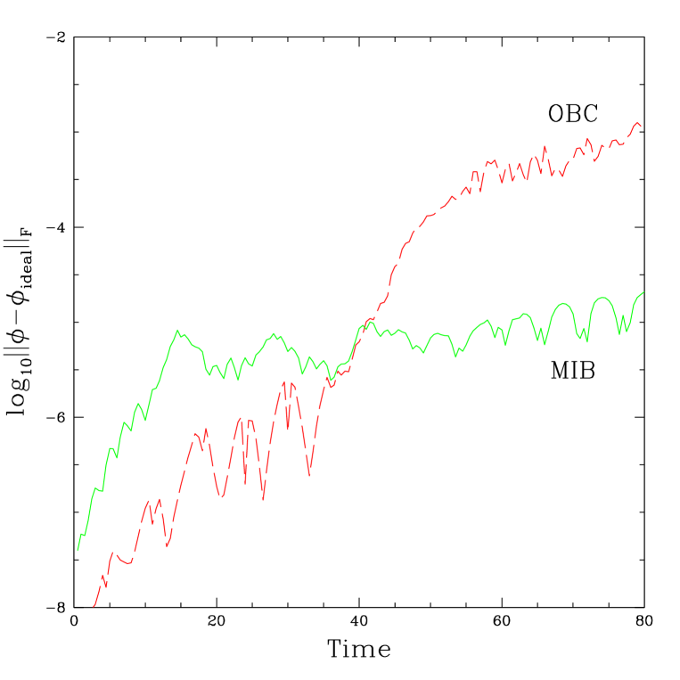
Figure 5.4: Plot comparing the OBC (dashed red) and MIB (solid green) solutions to an “ideal” solution. The OBC solution is obtained from using a massless outgoing boundary condition, the MIB solution is obtained by solving the system in axisymmetric MIB coordinates, and the ideal solution is obtained by evolving the solution in standard ($R$,$z$,$t$) coordinates on a grid large enough to ensure no reflection off the outer boundaries. The error estimates are obtained from the $\ell_{2}$-norm of the difference between the trial solutions (OBC or MIB) and the ideal solution, $||\phi-\phi_{\rm ideal}||_{F}$. Contamination of the OBC solution is observed at two crossing times, $t\approx 40$, where the error estimate increases almost three orders of magnitude.

Just like with the 1-D code, since the 2-D MIB code conserves energy quadratically, has quadratically convergent field variables, and is in agreement with the large-grid solution; it is an acceptable means of solving equations (5.5),(5.6),(5.7), and (5.8), while being dramatically more computationally efficient than either dynamical grid methods or large-grid methods. The computational demand for the MIB system grows linearly with the oscillon lifetime, while for dynamical or large-grid methods, the computational demand grows as the cube of the oscillon lifetime.

5.4 Boosting the Spherically Symmetric Oscillons as Initial Data

The main (certainly most fun) reason for creating an axisymmetric code to solve the KG equation was to investigate what happens when two oscillons collide.

The first step in most dynamical calculations is to generate meaningful initial data. Since there is no “closed-form” oscillon solution, it is actually non-trivial to generate “boosted” oscillon data. There are many approximate initial data configurations that give rise to a gaussian-shaped bubble that can move at the desired velocity. For example, “boosting”

$$\phi(\tilde{R},\tilde{z},\tilde{t})=\displaystyle{\phi_{0}\exp\left(-\frac{\tilde{R}^{2}}{\sigma_{R}^{2}}-\frac{\tilde{z}^{2}}{\sigma_{z}^{2}}\right)\sin\left(\omega\tilde{t}\right)}$$ (5.57)

by applying the coordinate transformation for a Lorentz boost along the z-axis (using $\displaystyle{\gamma=\frac{1}{\sqrt{1-v^{2}}}}$):

$$\phi(R,z,t)=\displaystyle{\phi_{0}\exp\left(-\frac{R^{2}}{\sigma_{R}^{2}}-\frac{\left(\gamma\left(z-vt\right)\right)^{2}}{\sigma_{z}^{2}}\right)\sin\left(\omega\gamma\left(t-vz\right)\right),}$$ (5.58)

usually results in an oscillon that moves at roughly the desired velocity. The problem, however, is that even with the best possible choices of the free parameters ($\phi_{0}$, $\omega$, $\sigma_{R}$, $\sigma_{z}$) the approximate oscillon (5.57) is not a solution to the (Lorentz invariant) Klein-Gordon equation. Therefore, trying to generate initial data in this manner often results in dramatically different global behavior depending on the “boost velocity”, $v$ (ie. behavior that is not Lorentz invariant and can be as dramatic as leaving the universe in different vacuum states!). The goal is to be able to compare oscillons being collided at different velocities while knowing exactly how each oscillon behaves in its own rest-frame.

We choose to numerically evolve the oscillon in its rest frame (which can be done efficiently in spherical symmetry) and then numerically boost the solution. The single boosted oscillon then, of course, retains all of its Lorentz invariant properties regardless of boost velocity. The collision initial data is constructed from the superposition of two boosted oscillons (one at some $z<0$ boosted in the $z^{+}$ direction, and the other at some $z>0$ boosted in the $z^{-}$ direction).

The equations for the transformation between the boosted (tilde) and rest (non-tilde) frames are just the equations for a Lorentz boost along the z-axis:

$$\begin{array}[]{rclcrcl}\tilde{t}&=&\gamma\left(t-vz\right)&&t&=&\gamma\left(\tilde{t}+v\tilde{z}\right)\\ \tilde{z}&=&\gamma\left(z-vt\right)&&z&=&\gamma\left(\tilde{z}+v\tilde{t}\right)\\ \tilde{R}&=&R&&R&=&\tilde{R}\\ \tilde{\theta}&=&\theta&&\theta&=&\tilde{\theta}\end{array}$$ (5.59)

where again, $\displaystyle{\gamma=\frac{1}{\sqrt{1-v^{2}}}}$. Since $\phi$ is a scalar field, it transforms trivially as

$$\tilde{\phi}(\tilde{t},\tilde{R},\tilde{\theta},\tilde{z})=\phi\left((\gamma\left(t-vz\right),R,\theta,\gamma\left(z-vt\right)\right),$$ (5.60)

while the other field variables (being derivatives of the scalar field) transform as forms $\partial_{\mu^{\prime}}\phi=\displaystyle{\frac{\partial x^{\mu}}{\partial x^{\mu^{\prime}}}\partial_{\mu}\phi}$ which gives

$$\begin{array}[]{rcl}\tilde{\Pi}&=&\displaystyle{\gamma\Pi+\gamma v\Phi_{z}}\\ &=&\displaystyle{\gamma\Pi+\frac{\gamma vz}{\sqrt{R^{2}+z^{2}}}\Phi_{r}}.\\ \end{array}$$ (5.61)

where $\Phi_{r}=\partial_{r}\phi$ and is obtained from the spherically symmetric evolution. (Remember that $r\equiv\displaystyle{\sqrt{x^{2}+y^{2}+z^{2}}}$ and $R\equiv\displaystyle{\sqrt{x^{2}+y^{2}}}$.)

Equations (5.59) imply that to obtain data for $\tilde{t}=0$, $\tilde{R}_{\rm min}\leq\tilde{R}\leq\tilde{R}_{\rm max}$, and $\tilde{z}_{\rm min}\leq\tilde{z}\leq\tilde{z}_{\rm max}$, the rest frame solution must be known over the spacetime domain $\gamma v\tilde{z}_{\rm min}\leq t\leq\gamma v\tilde{z}_{\rm max}$, $\tilde{R}_{\rm min}\leq R\leq\tilde{R}_{\rm max}$, and $\gamma\tilde{z}_{\rm min}\leq z\leq\gamma\tilde{z}_{\rm max}$. Time symmetric initial data was used and the $z$ domain was chosen such that $\tilde{z}_{\rm min}=-\tilde{z}_{\rm max}$ which allowed the time domain for the spherical evolution to be restricted to $0\leq t\leq\gamma\,v\,\tilde{z}_{\rm max}$ (see figure 5.5 for a schematic relating a “new” $t=0$ slice to the “old” spacetime ($\tilde{t}$,$\tilde{z}$) domain, for a typical $R={\rm constant}$ slice).

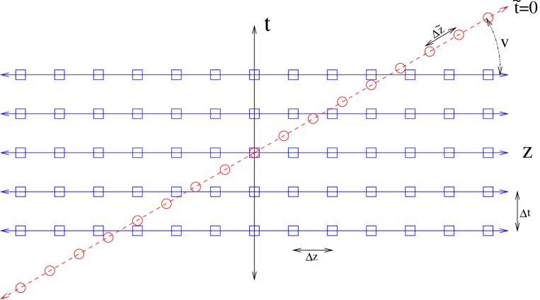
Figure 5.5: A schematic (for a sample constant-$R$ slice) displaying how the ($R$,$\tilde{z}$,$\tilde{t}_{0}$) boosted data is obtained by interpolating from rest-frame ($R$, $z$,$t$) dynamic data. Data points that do not match up exactly between the tilde and non-tilde frames are linearly interpolated in both space and time (note that figure is only a schematic and not drawn to scale, $\Delta z$ and $\Delta t$ were always taken to be very small compared to $\Delta\tilde{z}$). The blue squares are gridpoints lying on $t$-constant hypersurfaces in the rest-frame. Red circles are gridpoints lying on the $\tilde{t}=0$ boosted-frame hypersurface (the initial data being obtained). To obtain boosted data for $\tilde{z}_{min}\leq\tilde{z}\leq\tilde{z}_{max}$ at $\tilde{t}=0$, the rest-frame radius must be known over the domain $\gamma v\tilde{z}_{min}\leq t\leq\gamma v\tilde{z}_{max}$ and $\gamma\tilde{z}_{min}\leq z\leq\gamma\tilde{z}_{max}$. Since $R$ and $\tilde{R}$ are orthogonal to the boost, the field remains unaffected in that direction.

A boosted oscillon can then be obtained by time evolving the desired (rest frame) oscillon throughout the necessary spacetime domain and transforming the field variables using equations (5.60,LABEL:pitrans). Since very few of the ($t$, $R$, $z$) gridpoints match exactly any gridpoint from the spherically symmetric ($t$,$r$) grid, linear interpolation in both space and time was used (the 1-D grid that was interpolated from is at a much finer resolution than the 2-D grid). A schematic of an constant-$R$ slice can be seen in figure 5.5. Finally, collision initial data is obtained by forming the superposition of two boosted oscillons (obviously, boosted at one another.).

5.4.1 Testing the Numerically Boosted Initial Data

The “numerical boosting” of the spherically symmetric oscillon data was tested by monitoring the Lorentz invariant behavior of expanding bubble formation. For a spherically symmetric gaussian pulse, instantaneously at rest,

$$\phi(r,0) = \phi_{F}+\left(\phi_{T}-\phi_{F}\right)\exp\left(-\frac{r^{2}}{\sigma_{r}^{2}}\right)$$ (5.62)

$$\vbox{\vspace{0.75cm}}\dot{\phi}(r,0) = 0$$ (5.63)

so $\phi(\infty,t)=\phi_{F}$ and $\phi(0,t)=\phi_{T}$, there will be a critical “bubble radius”, $\sigma_{r}^{*}$, for which time evolution of $\sigma_{r}>\sigma_{r}^{*}$ will lead to an expanding bubble that converts false vacuum to true vacuum everywhere. For $\sigma_{r}<\sigma_{r}^{*}$ the time evolution will eventually result in dispersal of the field (possibly after an oscillon stage). Since $\sigma_{r}^{*}$ is defined to be the rest-frame critical radius for expanding bubble formation, this number should not change and the boosting of the critical field configuration should always lie on the threshold of expanding bubble formation.

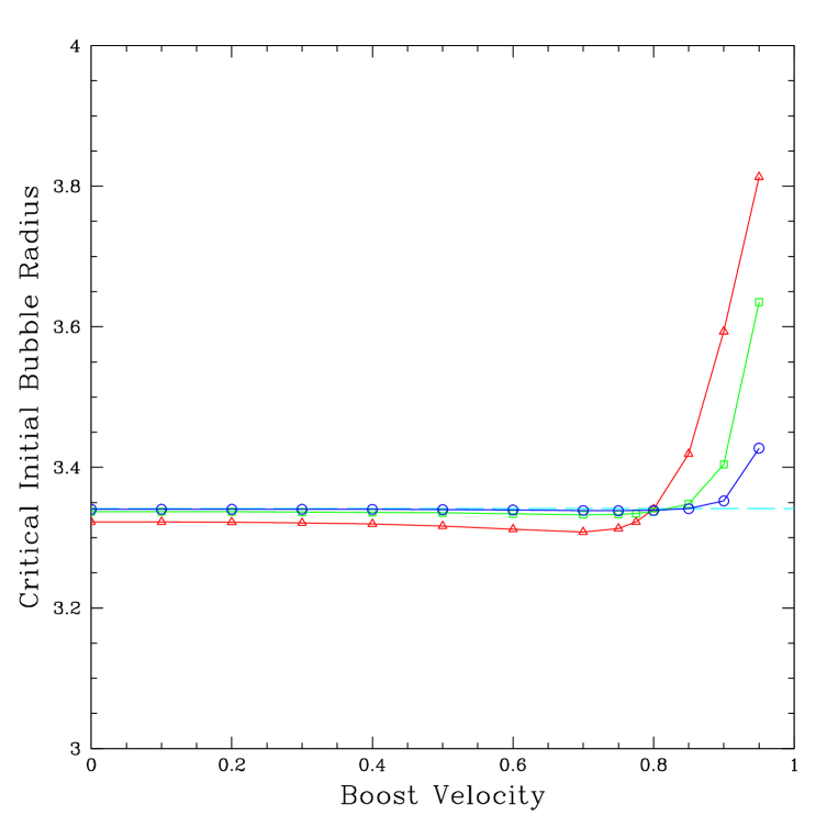
Figure 5.6: Plot of the Critical Initial Bubble Radius versus Boost Velocity for three discretizations ($81\times 161$ in red triangle, $161\times 321$ in green squares, and $321\times 641$ in blue circles). Since the initial bubble radius parameter in the code is the rest-frame initial radius, the Lorentz invariant behavior of contraction or expansion (which governs the threshold value of $r_{0}$) should not change as a function of boost velocity. The “ideal” result is the (dashed cyan) horizontal line at $r_{0}\approx 3.34$ (determined spherically symmetric collapse at $N_{r}=2049$). The deviation at large boost velocity is due to the increasing effects of length contraction of the bubble.

Figure (5.6) shows the critical bubble radius as a function of boost velocity for three resolutions ($81\times 161$, $161\times 321$, $321\times 641$); the critical bubble radius remains constant to within one-quarter percent at $161\times 321$ for $v\leq 0.8$, and to within one percent at $v=0.85$. The three resolutions show convergent properties (ie. the graph of $\sigma_{r}^{*}$ vs. boost velocity approaches a constant as $h\rightarrow 0$) and suggest that the deviation from the expected value of $\sigma_{r}^{*}$ at high boost velocity is due to the steep gradients which primarily result from the length contraction of the bubble.

5.5 Collision and Endstate Detection

In the spherically symmetric ADWP collapse, there were two possible endstates: expanding bubble formation or bubble collapse (usually resulting in the formation of an oscillon). However, in axisymmetric collision simulations, there are four possible endstates that we consider: expanding bubble formation, annihilation, soliton-like transmission, and coalescence.

Expanding bubble formation occurs when the whole spacetime is converted from the (unstable) false vacuum to the (stable) true vacuum. This can occur trivially when the bubbles that are being boosted at one another each have initial rest-frame radii above the critical radius for expanding bubble formation (for $\delta=0.1$, $\sigma^{*}_{r}\approx 3.3$); this is the case where each bubble would lead to an expanding bubble independently. However, a more interesting case involves the collision of two oscillons, each with a rest-frame radius less than the critical radius for expanding bubble formation. In this case, each oscillon independently would not lead to an expanding bubble, but together they overcome the potential barrier of $V_{A}(\phi)$ and a false-to-true phase transition ensues (see figure 5.7 for heuristic explanation).

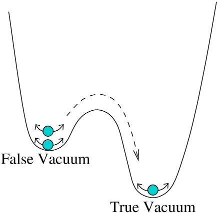
Figure 5.7: Heuristic representation of what happens energetically when two oscillons collide to form an expanding true vacuum bubble. Individually, the two bubble configurations (represented by the two balls oscillating about the false vacuum) are far from one another and do not individually have enough energy to overcome the potential barrier; if left alone, they would eventually disperse, leaving the spacetime in the false vacuum. However, when the two oscillons collide, their combined energy is enough overcome the potential barrier and form an expanding bubble that converts the spacetime to true vacuum. A time series of an actual collision of this type can be seen in figure 5.8.

The code detects bubble formation by computing the area (${\int dR\ dz}$, since we work in two spatial dimensions) that is in the true-vacuum and stopping the evolution after some empirically determined threshold is reached. In practice, it is quite easy to see where the “surface tension” in the bubble wall can no longer compete with the field’s “attraction” to the true-vacuum; the detection threshold is then taken to be safely above this point. A time series of snapshots of an actual 2-D collision that results in the formation of an expanding bubble can be seen in figure 5.8.

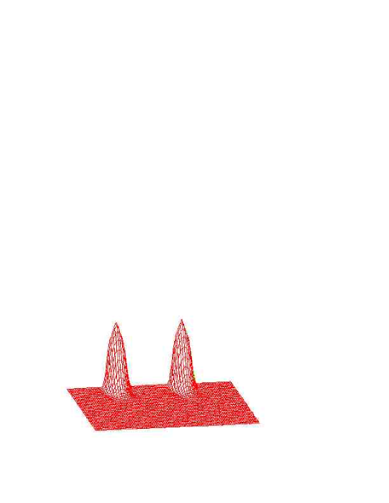
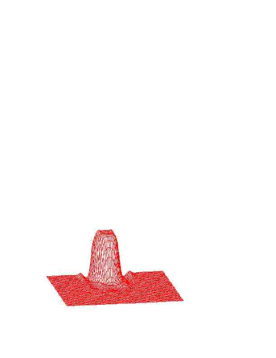
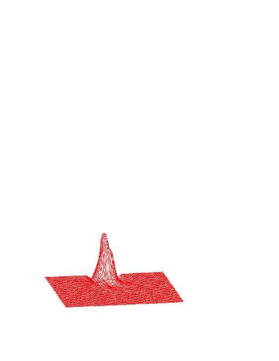
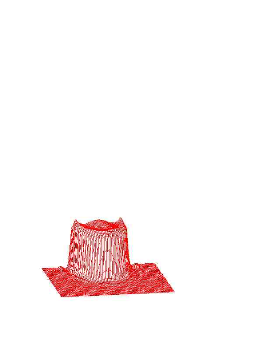
                      (a)                       (c)                       (b)                       (d)

Figure 5.8: A times series showing the collision of two oscillons forming an expanding true vacuum bubble. The initial frame (a) shows the two oscillons boosted toward one another; the fields interpolate between the vacua so that their peaks are at the true vacuum while away from the oscillons is the false vacuum. Frames (b) and (c) show the nonlinear interactions during the collision. Frame (d) shows the beginning of an expanding bubble; the steep field gradient is the bubble wall. Inside the bubble wall is the true vacuum and the bubble wall will continue to move outward (eventually reaching the speed of light).

The other three endstates being considered do not form expanding bubbles and therefore leave the spacetime in the false vacuum. Two of these three endstates, annihilation and soliton-like transmission are forms of dispersal, while coalescing oscillons remain within the computational domain. To help distinguish between these endstates, three second moments are considered:

$$M^{2}_{R}(t) = \displaystyle{\frac{\displaystyle{\int R^{2}\tilde{\rho}\ dR\ dz}}{\displaystyle{\int\tilde{\rho}\ dR\ dz}}}$$ (5.64)

$$M^{2}_{z}(t) = \frac{\displaystyle{\int z^{2}\tilde{\rho}\ dR\ dz}}{\displaystyle{\int\tilde{\rho}\ dR\ dz}}$$ (5.65)

$$M^{2}_{r}(t) = \frac{\displaystyle{\int\left(R^{2}+z^{2}\right)\tilde{\rho}\ dR\ dz}}{\displaystyle{\int\tilde{\rho}\ dR\ dz}}$$ (5.66)

where

$$\tilde{\rho}(R,z,t)=\displaystyle{\frac{1}{2}\left(\frac{\Pi^{2}}{a^{2}b^{2}}+\frac{\Phi_{R}^{2}}{a^{2}}+\frac{\Phi_{z}^{2}}{b^{2}}\right).}$$ (5.67)

$\tilde{\rho}$ is the energy density due to the time derivative and gradients of the field, neglecting the potential terms. Including the potential term would lead to large contributions to the moments from outside the bubble, whereas the goal here is to know the the location of the surface of the bubbles. For all of the collisions discussed here, the initial data are symmetric about the $z=0$ plane, and hence the collision also occurs at $z=0$.

Annihilation occurs when two oscillons collide and interact in such a way that the field is no longer localized and all the radiation disperses. The code determines this to be the endstate when both $M^{2}_{R}$ and $M^{2}_{z}$ rise above an empirically chosen threshold. This was typically taken to be around $100$ which implies most of the matter is around $r=\sqrt{R^{2}+z^{2}}=10$), which, in turn, is indicative of dispersal for oscillons with typical radii around $r\approx 3$. A time series of a collision resulting in annihilation can be seen in figure 5.9.

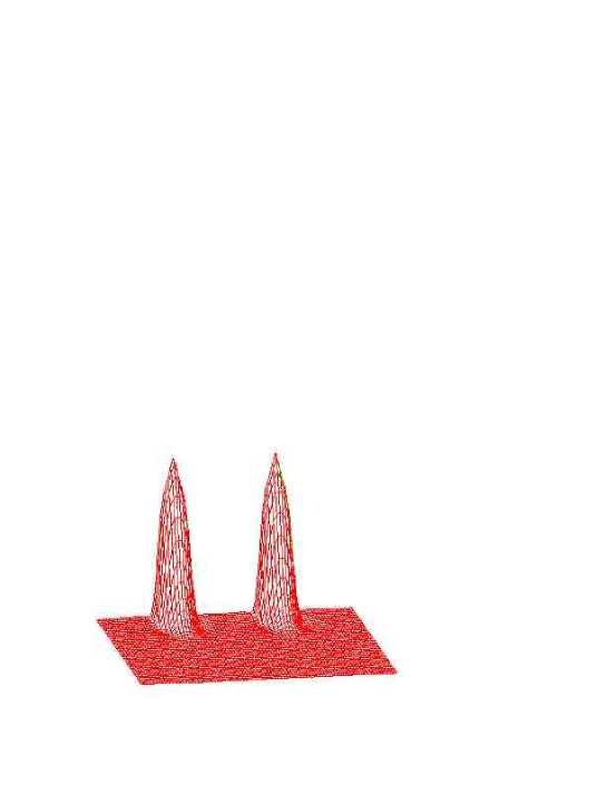
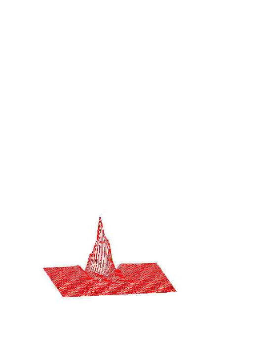
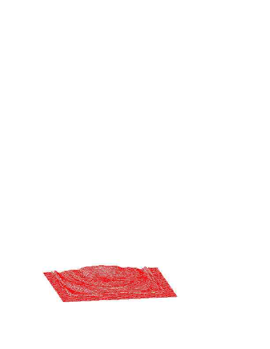
                      (a)                       (c)                       (b)                       (d)

Figure 5.9: A times series showing the collision of two oscillons that annihilate each other. The initial frame (a) shows the two oscillons boosted toward one another; the fields interpolate between the vacua so that their peaks are at the true vacuum while away from the oscillons is the false vacuum. Frames (b) and (c) show the nonlinear interactions during the collision. Frame (d) shows the endstate consisting of almost entirely of outgoing radiation. The spacetime is left in the false vacuum.

Soliton-like Transmission occurs when two oscillons collide, interact, and then pass through (or reflect off) one another while each oscillon stays localized.

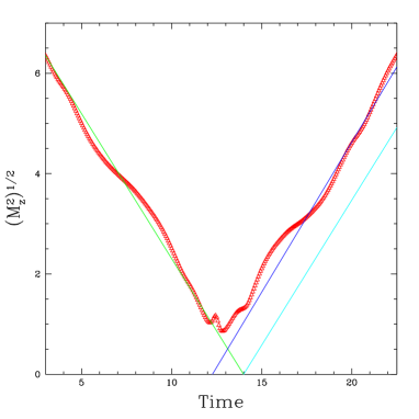
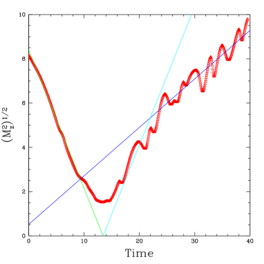
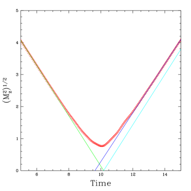
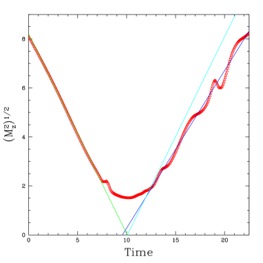
                 (a) $v_{b}=0.6$, $\sigma_{0}=2.15$                  (c) $v_{b}=0.6$, $\sigma_{0}=2.675$                    (b) $v_{b}=0.85$, $\sigma_{0}=2.0$                  (d) $v_{b}=0.85$, $\sigma_{0}=3.325$

Figure 5.10: Plots of the location, $(M^{2}_{z})^{1/2}$, of the oscillon located in the “upper” ($z>0$) half of the computational domain as a function of time. In either plot, the green line is the best fit for the ingoing position as a function of time, the blue line is the best fit for the outgoing position, and the cyan line is the path that the oscillon would have taken had it not interacted (nonlinearly) with the other oscillon (direct reflection across $z=0$). During the transmission the velocities (slopes) can increase or decrease while the outgoing path was always seen to be shifted backward in time (x-intercept always moved left). Table 5.1 shows the measured time lags and changes in velocity for these four evolutions.

Again, this is easily determined by monitoring the second moments. Since the oscillons pass through one another, the $z$ moment will get large as they leave the computational domain. However, since each oscillon remains localized, the $R$ moment will stay small (on the order of the typical oscillon radius of $r\approx 3$). A time series of a collision resulting in soliton-like transmission can be seen in figure 5.11.

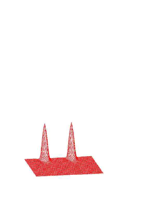
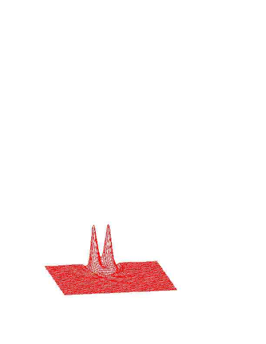
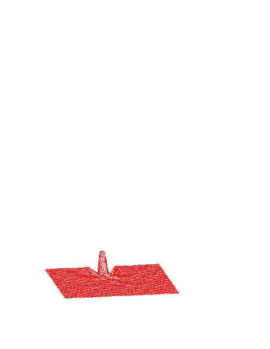
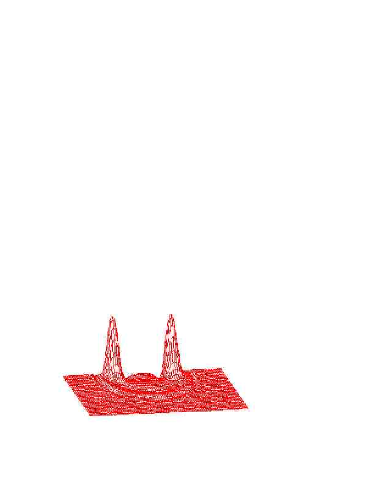
                      (a)                       (c)                       (b)                       (d)

Figure 5.11: A times series showing the collision of two oscillons that pass through (or reflect off) one another. The initial frame (a) shows the two oscillons boosted toward one another; the fields interpolate between the vacua so that their peaks are at the true vacuum while away from the oscillons is the false vacuum. Frames (b) and (c) show the nonlinear interactions during the collision. Frame (d) shows the endstate consisting of two oscillons moving outward along the $z$-axis. The spacetime is left in the false vacuum.

$v_{b}$ $\sigma_{0}$ $\Delta|v|$ $\Delta T$ 0.6 2.15 +0.02 -1.7 0.6 2.675 -0.41 -15.8 0.85 2.00 -0.02 -0.6 0.85 3.325 -0.17 -0.5

Table 5.1: Table of change in the oscillon velocity (magnitude), $\Delta|v|$, and time “lag”, $\Delta T$, for four sample soliton-like collisions. Oscillons (and solitons) that interact nonlinearly are usually characterized by a time shift or change in velocity arising from coupling between modes. If the oscillons interacted linearly, $\Delta|v|$ and $\Delta T$ would be zero. The oscillons explored here almost always slow down or stay at roughly the same speed and the time lag (measured by extrapolating back to $z=0$) almost always is negative. This is contrary to what is usually seen in (1+1) dimensional soliton interactions where $\Delta T>0$.

Lastly, Coalescence occurs when the two oscillons collide, interact, radiate away some of their energy, and survive to form a single oscillon.

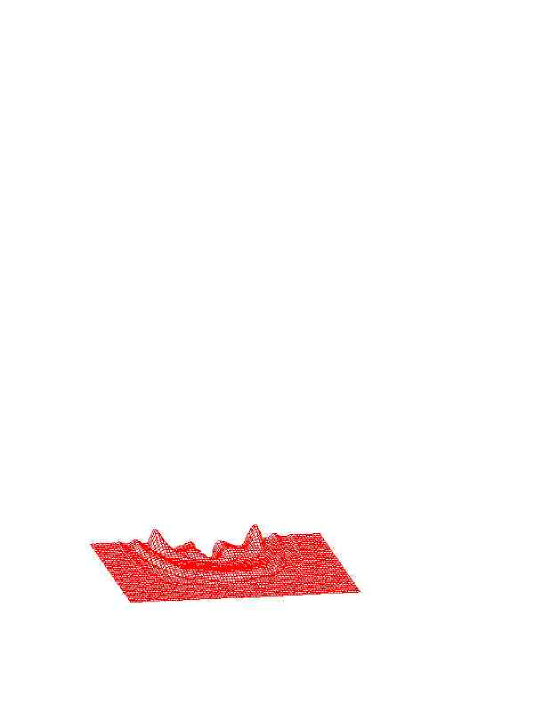
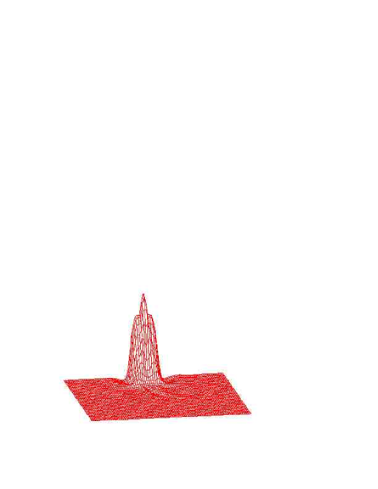
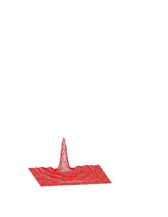
                      (a)                       (c)                       (b)                       (d)

Figure 5.12: A times series showing the collision of two oscillons that coalesce. The initial frame (a) shows the two oscillons boosted toward one another; the fields interpolate between the vacua so that their peaks are at the true vacuum while away from the oscillons is the false vacuum. Frames (b) and (c) show the nonlinear interactions during the collision, where roughly half the total energy of the system is converted into radiation. Frame (d) shows the endstate consisting of one remaining oscillon, oscillating on top of the false vacuum.

Coalescence is the default endstate for the code’s detection algorithm since it is what happens if an expanding bubble does not form or the field does not disperse in the form of annihilation or soliton-like transmission. Unfortunately, simulations with this endstate are the most computationally intensive because it is hard to know how long to wait before deciding that the solution will not disperse or form an expanding bubble (particularly on the threshold of expanding bubble formation). A time series of an oscillon-oscillon collision that results in coalescence can be seen in figure 5.12. The endstate classification logic is summed up in Table 5.2.

${\rm\left(Area\right)_{True\ Vacuum}}$ $M^{2}_{R}$ $M^{2}_{z}$ Expanding Bubble large – – Annihilation small large large Soliton-like small small large Coalescence small small small

Table 5.2: Logic table for endstate classification. ${\rm\left(Area\right)_{True\ Vacuum}}$ is the “area” ($\int dz\ dR$) of space that is in the true vacuum. $M^{2}_{R}$ and $M^{2}_{z}$ are the second $R$ and $z$ moments, respectively, of the energy density-like function, $\tilde{\rho}$. The expanding bubbles are easily separated from the other endstates; once the area of space at the true vacuum reaches a given threshold, the collision is flagged as forming an expanding bubble. Annihilation and soliton-like transmission both occur when the field disperses ($M^{2}_{z}$ becomes large) and are differentiated by the mass moment in the radial direction; if $M^{2}_{R}$ is small, the field is localized indicative of transmission, whereas if $M^{2}_{R}$ is large, the field has clearly dispersed.

5.6 Parameter Space Survey

In the spherically symmetric ADWP evolutions, a natural parameter to adjust in the exploration of the model was the initial width of the collapsing bubble, $\sigma_{r}$ of equation (5.62). This one dimensional parameter space is extended here by adding the boost velocity, $v_{b}$, as a second parameter. Although the initial data is still highly symmetric (the colliding oscillons are the same size and oscillate in phase), there is still interesting structure to the parameter space. In figure 5.13 we see that for a large area of parameter space, there are collisions where bubbles that would otherwise have (eventually) dispersed actually combine to form an expanding true vacuum bubble.

Figure 5.13: Two dimensional, $\sigma_{0}$-$v_{b}$, parameter space survey of axisymmetric bubble collisions (colored according to the endstate of the system); the vertical axis measures the initial rest-frame radius of the bubble, $\sigma_{0}$, while the horizontal axis measures the velocity that each oscillon is boosted at, $v_{b}$. The red region corresponds to expanding vacuum bubble formation, the cyan region to coalescence, the blue region to soliton-like transmission, and the green to annihilation. The black curve is the line representing the threshold for expanding bubble formation for individual boosted bubbles (bubbles above this line would form expanding vacuum bubbles even if not colliding). The black $\times$’s correspond to points on the threshold of expanding bubble formation for which critical phenomena was explored (see table 5.3). Each collision was performed on a 161x321 grid.

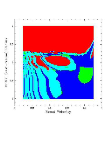
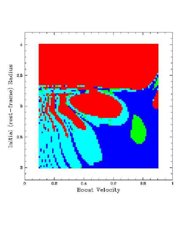
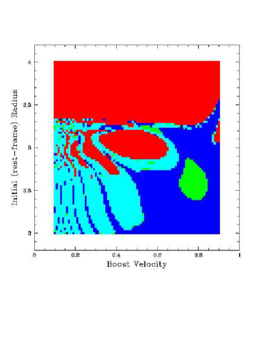
                      (a) $81\times 161$, $h=0.25$                       (c) $161\times 321$, $h=0.125$                       (b) $114\times 227$, $h\approx 0.177$                       (d) $227\times 453$, $h\approx 0.088$

Figure 5.14: $\sigma_{0}$-$v_{b}$ parameter space surveys at four different discretizations ($\Delta r=\Delta z=h$). Although no particular convergence factor was measured, the shapes of the colored regions appear to be converging to those of figure (d), at least well enough to support the existence of both the large oval-shaped red region centered around $v_{B}\approx 0.5$, $\sigma_{0}\approx 3$ and the side-lobes that are present for smaller boost velocities (to the left of the main oval).

5.7 Threshold of Expanding Bubble Formation in 2D Collisions
(2D Critical Phenomena)

At the end of chapter 4, a time scaling law was presented for solutions on the threshold of expanding bubble formation for spherically symmetric bubble collapse. With the 2D parameter space surveys presented in section 5.6 (for collisions), there also is a boundary separating expanding bubble formation from solutions that leave the space in the false vacuum. The natural question is then: Does a similar scaling law exist, and if so, does it have the same critical exponent?

The threshold of expanding bubble formation was explored first by fixing the boost velocity, $v_{b}$, and then bisecting between two values of the initial rest frame radius, $\sigma_{r}$ (one that forms an expanding vacuum bubble and one that does not). Next, the threshold was explored along a different direction in parameter space by fixing $\sigma_{r}$ and bisecting between two values of $v_{b}$. Time scaling relations were observed for each bisection and the critical exponents were observed to be quite similar ($\gamma\approx 2.2$, see table 5.3). The locations in parameter space of these critical points can be seen by the crosses in figure 5.13. The similarity between the critical exponents for the axisymmetric collision of two gaussian bubbles and the spherically symmetric collapse of a single gaussian bubble suggests that the dominant unstable mode observed with the axisymmetric critical solution might be spherically symmetric.

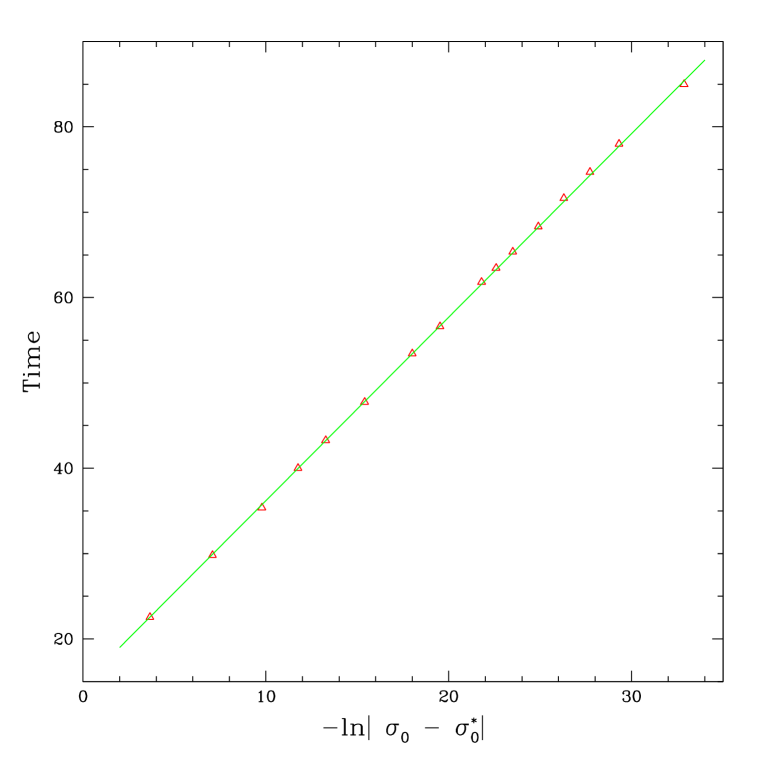
Figure 5.15: Sample Time versus $-\ln|\sigma_{0}-\sigma^{*}_{0}|$ plot for the threshold of expanding bubble formation. The points plotted are for $\sigma_{0}>\sigma^{*}_{0}$ and therefore all produce expanding bubbles. The scaling exponent (slope) was measured to be $\gamma\approx 2.15$. All of the threshold parameters explored produced similar scaling exponents and are tabulated in figure 5.3.

$\sigma^{*}_{r}$ $\Delta\sigma$ $v^{*}_{b}$ $\Delta v^{*}_{b}$ $\gamma$ 2.620314246044920 $\sim 10^{-14}$ 0.4 fixed 2.18 2.824162086503015 $\sim 10^{-14}$ 0.5 fixed 2.15 2.813209312722570 $\sim 10^{-14}$ 0.6 fixed 2.19 3.293020631075245 $\sim 10^{-14}$ 0.6 fixed 2.15 3.281889627766725 $\sim 10^{-14}$ 0.7 fixed 2.15 3.270433308449535 $\sim 10^{-14}$ 0.75 fixed 2.15 3.278874383866785 $\sim 10^{-14}$ 0.8 fixed 2.17 2.5 fixed 0.292882455348505 $\sim 10^{-14}$ 2.18 2.6 fixed 0.206552206744452 $\sim 10^{-14}$ 2.18 2.65 fixed 0.415868755640645 $\sim 10^{-14}$ 2.17 2.7 fixed 0.337408336301504 $\sim 10^{-14}$ 2.17 3.0 fixed 0.658702864946936 $\sim 10^{-14}$ 2.20 3.0 fixed 0.327480589060684 $\sim 10^{-14}$ 2.17 3.2 fixed 0.546131322091751 $\sim 10^{-14}$ 2.19

Table 5.3: Table of critical exponents and threshold parameter values for a two-dimensional parameter space survey of axisymmetric collisions. The entire survey can be seen in figure 5.13, where the black x’s denote the threshold values in this table. The points were chosen to span the space as much as possible and the bisection search was performed in both directions of the parameter space; nevertheless the critical exponents are remarkably similar, suggesting a universal scaling law (see figure 5.15).

Chapter 6 Trial Function Approach to Critical Solutions

This chapter discusses both exact and approximate critical (non-radiative) oscillon solutions obtained through a trial function approach. Differential equations (4.25) and (4.26) are rederived using a very general trial function ansatz. By assuming more constrained gaussian and hyperbolic secant trial functions, approximate critical oscillon solutions are also obtained.

6.1 Trial Functions & Variational Approach

In section 4.4.2, the ordinary differential equations (4.25) and (4.26) were derived by inserting the ansatz

$$\phi(r,t)=-1+\phi_{0}(r)+\sum_{n=1}^{\infty}\phi_{n}(r)\cos\left(n\omega t\right)$$ (6.1)

into the equation of motion (4.2) and matching $\cos(n\omega t)$ terms. The same set of differential equations can be obtained by inserting (6.1) into the action

$$\begin{array}[]{rcl}S&=&\displaystyle{\int d^{4}x\ {\mathcal{L}}}\\ &=&\displaystyle{4\pi\int r^{2}\left(\frac{1}{2}\left(\dot{\phi}\right)^{2}-\frac{1}{2}\left(\phi^{\prime}\right)^{2}-\frac{1}{4}\left(\phi^{2}-1\right)^{2}\right)dr\ dt}\end{array}$$ (6.2)

and integrating over time to obtain a dimensionally reduced action. The reduced action is then varied with respect to the individual modes, $\phi_{0}$ and $\phi_{n}$, to obtain the (ordinary differential) equations of motion.

Ansatz (4.24,6.1) is actually obtained by starting with the most general possible ansatz

$$\phi(r,t)=-1+\phi_{0}(r)+\sum_{n=1}^{\infty}A_{n}(r)\sin\left(n\omega t+\theta_{n}\right)$$ (6.3)

and imposing boundary conditions that match the phases of the each mode and that demand that the maximum amplitude of each mode is equal to $A_{n}(0)$. The reduced action obtained by integrating (6.2) and (6.1) over time is

$$\begin{array}[]{rclcl}S&=&\displaystyle{4\pi\int^{\infty}_{r=0}dr\int^{T}_{t=0}\ {\mathcal{L}}{(r,t)\hbox{}}}&&\\ &=&\vbox{\vspace{1cm}}\displaystyle{\frac{4\pi^{2}}{\omega}\int^{\infty}_{r=0}dr}&\left\{\vbox{\vspace{0.75cm}}\right.\hbox{}&\displaystyle{\frac{1}{2}\omega^{2}\sum^{\infty}_{n=1}n^{2}\phi_{n}^{2}-\left(\phi_{0}^{\prime}\right)^{2}-\frac{1}{2}\sum^{\infty}_{n=1}\left(\phi_{n}^{\prime}\right)^{2}}\\ &&&&\displaystyle{-\frac{1}{2}\phi_{0}^{2}\left(\phi_{0}-2\right)^{2}-\frac{1}{4}\left(6\phi_{0}^{2}-12\phi_{0}+4\right)\sum^{\infty}_{n=1}\left(\phi_{n}\right)^{2}}\\ &&&&\displaystyle{-\frac{1}{2}\left(\phi_{0}-1\right)\sum^{\infty}_{n,p,q=1}\phi_{n}\phi_{p}\phi_{q}\left(\delta_{n,\pm p\pm q}\right)}\\ &&&&\displaystyle{\left.-\frac{1}{16}\sum^{\infty}_{n,m,p,q=1}\phi_{n}\phi_{m}\phi_{p}\phi_{q}\left(\delta_{n,\pm m\pm p\pm q}\right)\right\}}\\ &=&\displaystyle{\frac{4\pi^{2}}{\omega}\int^{\infty}_{r=0}dr\ {\mathcal{L}}(r)\hbox{}}&&\\ &&&&\end{array}$$ (6.4)

where again the pluses and minuses sum over every permutation (ie. $\delta_{n,\pm p\pm q}=\left(\delta_{n,+p+q}+\delta_{n,+p-q}+\delta_{n,-p+q}+\delta_{n,-p-q}\right)$). Unfortunately, ansatz (6.1) is so general that the spatial integration cannot be done in closed-form. However, one can still vary the (partially) reduced action with respect to $\phi_{0}$ and $\phi_{n}$ to obtain the usual Euler-Lagrange equations,

$$\displaystyle{\partial_{\mu}\left(\frac{\partial{\mathcal{L}}(r)}{\partial\left(\partial_{\mu}\phi_{0}\right)}\right)-\frac{\partial{\mathcal{L}}(r)}{\partial\phi_{0}}} = 0$$ (6.5)

$$\displaystyle{\partial_{\mu}\left(\frac{\partial{\mathcal{L}}(r)}{\partial\left(\partial_{\mu}\phi_{n}\right)}\right)-\frac{\partial{\mathcal{L}}(r)}{\partial\phi_{n}}} = 0,$$ (6.6)

to obtain a set of differential equations which (again) are

$$\begin{array}[]{rcl}\frac{1}{r^{2}}\left(r^{2}\phi_{0}^{\prime}\right)^{\prime}&=&\phi_{0}\left(\phi_{0}-1\right)\left(\phi_{0}-2\right)\\ &&+\frac{3}{2}\left(\phi_{0}-1\right)\sum\limits_{n}\left(\phi_{n}\right)^{2}\\ &&+\frac{1}{4}\sum\limits_{n,p,q}\phi_{n}\phi_{p}\phi_{q}\left(\delta_{n,\pm p\pm q}\right),\end{array}$$ (6.7)

$$\begin{array}[]{rcl}\frac{1}{r^{2}}\left(r^{2}\phi_{n}^{\prime}\right)^{\prime}&=&\left(3\left(\phi_{0}-1\right)^{2}-\left(n^{2}\omega^{2}+1\right)\right)\phi_{n}\\ &&+\frac{3}{2}\left(\phi_{0}-1\right)\sum\limits_{p,q}\phi_{p}\phi_{q}\left(\delta_{n,\pm p\pm q}\right)\\ &&+\frac{1}{4}\sum\limits_{m,p,q}\phi_{m}\phi_{n}\phi_{q}\left(\delta_{n,\pm m\pm p\pm q}\right),\end{array}$$ (6.8)

respectively. The solution to equations (6.7) and (6.8) for $\omega=1.38$ can be seen in Figure 4.12. The solution matches extremely well to the Fourier decomposed dynamic data. Again, this is not surprising because the only assumption made restricting the ansatz that could prevent solutions to (6.7) and (6.8) from being solutions to the true PDE equations of motion was that the solution is periodic, a property which is observed empirically for the resonant oscillons.

6.2 Approximate Oscillons From Constrained Ansatz

Although the resonant non-radiative solutions found in section 6.1 match the dynamic data extremely well, they are still obtained from solving ordinary differential equations. With a well chosen and more constrained trial function, both the time and space integrations in the action can be evaluated in closed-form. Variational methods are then applied to obtain a set of algebraic equations that can be solved to obtain the best possible values for the free parameters of the trial function. The ansatz is taken to be

$$\phi(r,t)=-1+A\ f\left(\frac{r}{\sigma}\right)\sin\left(\omega t+\theta\right),$$ (6.9)

where $\sigma$ is related to the width of the field configuration and $A$ is the amplitude of the oscillations. Equation (6.9) is subjected to the following boundary conditions:

$$\phi(r,0) = -1$$ (6.10)

$$\phi(r,\pi/(2\omega)) = -1+Af\left(\frac{r}{\sigma}\right),$$ (6.11)

which results in a choice of phase, $\theta=0$, and sets $A$ equal to the maximum amplitude of the oscillating mode. This yields

$$\phi(r,t)=-1+A\ f\left(\frac{r}{\sigma}\right)\sin\left(\omega t\right)$$ (6.12)

for the general form of the trial function. Equation (6.12) is inserted into the action and can be written in terms of definite integrals.

$$\begin{array}[]{rcl}S&=&\displaystyle{4\pi\int^{\infty}_{0}dr\int^{\pi/(2\omega)}_{0}dt\ r^{2}\left\{\frac{1}{2}\dot{\phi}^{2}-\frac{1}{2}\phi^{\prime 2}-\frac{1}{2}\left(\phi^{2}-1\right)^{2}\right\}}\\ &=&\displaystyle{\vbox{\vspace{0.75cm}}\pi\left\{2A^{2}\sigma^{3}\omega c_{2}g_{1}-\omega^{-1}\left(2A^{2}\sigma c_{1}g_{2}+4A^{2}\sigma^{3}c_{2}g_{2}-4A^{3}\sigma^{3}c_{3}g_{3}+A^{4}\sigma^{3}c_{4}g_{4}\right)\right\}}\end{array}$$ (6.13)

where the $c_{i}$ are dimensionless constants

$$\begin{array}[]{rclcrcl}c_{1}&\equiv&\displaystyle{\int^{\infty}_{0}du\ u^{2}\left(\partial_{u}f(u)\right)^{2}}&\hbox{\hskip 28.45274pt}&c_{2}&\equiv&\displaystyle{\int^{\infty}_{0}du\ u^{2}f(u)^{2}}\\ \vbox{\vspace{0.75cm}}c_{3}&\equiv&\displaystyle{\int^{\infty}_{0}du\ u^{2}f(u)^{3}}&&c_{4}&\equiv&\displaystyle{\int^{\infty}_{0}du\ u^{2}f(u)^{4}}\end{array}$$ (6.14)

obtained by taking $u\equiv r/\sigma$ and the $g_{i}$ are dimensionless constants

$$\begin{array}[]{rcccl}g_{1}&\equiv&\displaystyle{\int^{\pi/2}_{0}d\tau\ \cos^{2}(\tau)}&=&\displaystyle{\frac{\pi}{4}}\\ \vbox{\vspace{0.75cm}}g_{2}&\equiv&\displaystyle{\int^{\pi/2}_{0}d\tau\ \sin^{2}(\tau)}&=&\displaystyle{\frac{\pi}{4}}\\ \vbox{\vspace{0.75cm}}g_{3}&\equiv&\displaystyle{\int^{\pi/2}_{0}d\tau\ \sin^{3}(\tau)}&=&\displaystyle{\frac{2\pi}{3}}\\ \vbox{\vspace{0.75cm}}g_{4}&\equiv&\displaystyle{\int^{\pi/2}_{0}d\tau\ \sin^{4}(\tau)}&=&\displaystyle{\frac{3\pi}{16}}\end{array}$$ (6.15)

obtained by taking $\tau\equiv\omega t$. The reduced action (6.13) will be the same even if $\sin(\omega t)$ in equation (6.12) is replaced with an arbitrary function, $h(\omega t)$. However, the constants, $g_{1}$, $g_{2}$, $g_{3}$, and $g_{4}$, will have to be recomputed according to

$$\begin{array}[]{rclcrcl}g_{1}&\equiv&\displaystyle{\int^{\tau_{1}}_{\tau_{0}}d\tau\ \left(\partial_{\tau}h(\tau)\right)^{2}}&\hbox{\hskip 28.45274pt}&g_{2}&\equiv&\displaystyle{\int^{\tau_{1}}_{\tau_{0}}d\tau\ h(\tau)^{2}}\\ \vbox{\vspace{0.75cm}}g_{3}&\equiv&\displaystyle{\int^{\tau_{1}}_{\tau_{0}}d\tau\ h(\tau)^{3}}&&g_{4}&\equiv&\displaystyle{\int^{\tau_{1}}_{\tau_{0}}d\tau\ h(\tau)^{4}}\end{array}$$ (6.16)

and the limits of integration need to be chosen appropriately.

Now that the action is completely reduced, varying with respect to the free parameters yields a system of algebraic equations,

$$\displaystyle{\frac{\partial S}{\partial\sigma}} = 0$$ (6.17)

$$\displaystyle{\frac{\partial S}{\partial A}} = 0,$$ (6.18)

that can be solved for $A$ and $\sigma^{2}$,

$$A_{\pm} = \displaystyle{\frac{6c_{3}g_{3}\pm\sqrt{36c_{3}^{2}g_{3}^{2}-16c_{2}c_{4}g_{4}\left(2g_{2}-g_{1}\omega^{2}\right)}}{2c_{4}g_{4}}}$$ (6.19)

$$\vbox{\vspace{0.75cm}}\sigma^{2}_{\pm} = \displaystyle{\frac{-2c_{1}g_{2}}{3\left(c_{4}g_{4}A_{\pm}^{2}-4c_{3}g_{3}A_{\pm}+2c_{2}\left(2g_{2}-g_{1}\omega^{2}\right)\right)}}.$$ (6.20)

The reader may be wondering why, since the action is also a function of $\omega$, that the equation $\displaystyle{\frac{\partial S}{\partial\omega}=0}$ was not added to the system of equations, (6.17) and (6.18). Unfortunately, the trial function method does not work well to determine $\omega$. Looking at typical plots of the action as a function of the amplitude and width (figures 6.1 and 6.2, respectively), it is apparent that there are no (non-trivial) points where $\displaystyle{\frac{\partial S}{\partial\omega}=0}$. Forcing this equation to be solved in conjunction with (6.17) and (6.18) results in unphysical complex solutions. In the following subsections, we choose three forms for $f(r/\sigma)$ and look at the amplitude and widths as a function of $\omega$.

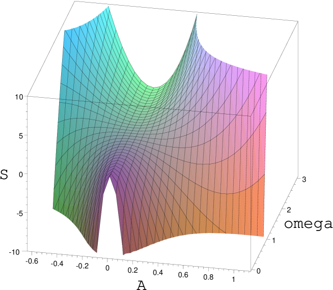
Figure 6.1: Plot of the reduced action as a function of the oscillon amplitude, $A$, and the frequency, $\omega$ (while setting $\sigma=3.6$). Looking along $\omega$-constant slices, it is clear that there are many points that satisfy $\displaystyle{\frac{\partial S}{\partial A}=0}$, whereas when looking at $A$-constant slices, there are no points that satisfy $\displaystyle{\frac{\partial S}{\partial\omega}=0}$ (except for the trivial $A=0$ solution).

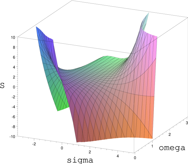
Figure 6.2: Plot of the reduced action as a function of the oscillon width, $\sigma$, and the frequency, $\omega$ (while setting $A=0.62$). Looking along $\omega$-constant slices, it is clear that there are many points that satisfy $\displaystyle{\frac{\partial S}{\partial\sigma}=0}$, whereas when looking at $\sigma$-constant slices, there are no points that satisfy $\displaystyle{\frac{\partial S}{\partial\omega}=0}$ (except for the trivial $\sigma=0$ solution).

6.2.1 Gaussian Trial Functions

In this subsection the field configuration is assumed to have a gaussian shape (as assumed in [24]),

$${f\left(\frac{r}{\sigma}\right)=\exp\left(-\frac{r^{2}}{\sigma^{2}}\right)}.$$ (6.21)

Now that $f(r/\sigma)$ has been chosen, the integrals (6.16) can now be performed:

$$\begin{array}[]{rclcrcl}\vbox{\vspace{0.75cm}}c_{1}&=&\displaystyle{\frac{3}{8}\sqrt{\frac{\pi}{2}}}&\hbox{\hskip 28.45274pt}&c_{2}&=&\displaystyle{\frac{1}{8}\sqrt{\frac{\pi}{2}}}\\ \vbox{\vspace{0.75cm}}c_{3}&=&\displaystyle{\frac{1}{12}\sqrt{\frac{\pi}{3}}}&&c_{4}&=&\displaystyle{\frac{1}{32}\sqrt{\pi}}.\end{array}$$ (6.22)

Using equations (6.19) and (6.20), $A_{\pm}$ and $\sigma^{2}_{\pm}$ can be plotted as a function of $\omega$ (figure 6.3). Unfortunately, for $\omega<0.437$ the discriminant in equation (6.19) is negative and gives complex solutions. Furthermore, where $A_{-}$ is real $\sigma^{2}_{-}$ is negative, resulting in an imaginary oscillon width! However, there is a part of the “+” root ($0.62<\omega<1.41$) that has positive $\sigma^{2}_{+}$ and can therefore support physical solutions. Table 6.1 compares sample solutions (located near the x’s in figure 6.3) to estimates obtained from the dynamic solution.

Dynamic Parameter Solution $A_{+}=A_{D}$ $\sigma_{+}=\sigma_{D}$ $A$ 0.62 0.62 0.39 $\sigma$ 3.6 2.9 3.6 $\omega$ 1.4 1.26 1.32

Table 6.1: Table of free parameter values ($A$, $\sigma$, and $\omega$) determined using a gaussian trial function (third and fourth columns) compared to the values estimated from the spherically symmetric dynamics (second column); the ${\rm D}$ subscript indicates the value was obtained from the dynamic solution. The third column contains results obtained using the trial function approach where $A_{+}$ equals the amplitude of the $n=1$ mode dynamic solution; the fourth column contains results where $\sigma_{+}$ equals the width of the $n=1$ mode dynamic solution. The data from the third and fourth columns occur around the x’s in figure 6.3.

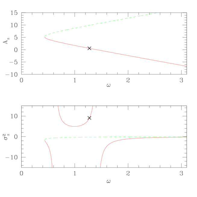
Figure 6.3: Plot of $A_{\pm}$ (top) and $\sigma^{2}_{\pm}$ (bottom) as a function of $\omega$ for gaussian $f(r/\sigma)$. The “+” roots are plotted in dashed green, while the “–” roots are plotted in solid red. The solution is not plotted for $\omega<0.437$ as the discriminant in equation (6.19) is negative and only real $A$ are of interest. The “+” roots are all unphysical since $\sigma^{2}_{+}$ is less than zero everywhere, which means that solutions within this region have an imaginary width. The solution for $\sigma^{2}_{-}$ is also unphysical outside the region $0.62<\omega<1.41$ for the same reason. Fortunately, there are solutions that are both physical (real roots) and similar to those seen in the dynamic simulations (near the x’s).

6.2.2 Hyperbolic Secant Trial Functions

In this subsection the field configuration is assumed to have a hyperbolic secant shape,

$${f\left(\frac{r}{\sigma}\right)={\rm sech}\left(\frac{r}{\sigma}\right)}.$$ (6.23)

With the new choice of $f(r/\sigma)$, the integrals (6.16) are now reevaluated:

$$\begin{array}[]{rclcrcl}\vbox{\vspace{0.75cm}}c_{1}&=&\displaystyle{\frac{1}{36}\pi^{2}+\frac{1}{3}}&\hbox{\hskip 28.45274pt}&c_{2}&=&\displaystyle{\frac{1}{12}\pi^{2}}\\ \vbox{\vspace{0.75cm}}c_{3}&=&0.3670959657&&c_{4}&=&\displaystyle{\frac{1}{18}\pi^{2}-\frac{1}{3}}.\end{array}$$ (6.24)

Using equations (6.19) and (6.20), the new $A_{\pm}$ and $\sigma^{2}_{\pm}$ are plotted as a function of $\omega$ (figure 6.4). Complex solutions exist for $\omega<0.595$ where (as with the gaussian trial function) the discriminant in (6.19) is negative. The ${\rm sech}$ function also yields unphysical solutions for all of the “–” roots since $\sigma^{2}_{-}$ is negative everywhere. Again, there is a part of the “+” solution ($0.73<\omega<1.41$) that has positive $\sigma^{2}_{+}$ and can therefore support physical solutions. Table 6.2 compares sample solutions (located near the x’s in figure 6.4) to estimates obtained from the dynamic solution.

Dynamic Parameter Solution $A_{+}=A_{D}$ $\sigma_{+}=\sigma_{D}$ $A$ 0.62 0.62 0.72 $\sigma$ 2.2 2.5 2.2 $\omega$ 1.4 1.29 1.27

Table 6.2: Table of free parameter values ($A$, $\sigma$, and $\omega$) determined using a ${\rm sech}$ trial function (third and fourth columns) compared to the values estimated from the spherically symmetric dynamics (second column); the ${\rm D}$ subscript indicates the value was obtained from the dynamic solution. The third column contains results obtained using the trial function approach where $A_{+}$ equals the amplitude of the $n=1$ mode dynamic solution; the fourth column contains results where $\sigma_{+}$ equals the width of the $n=1$ mode dynamic solution. The data from the third and fourth columns occur around the x’s in figure 6.4.

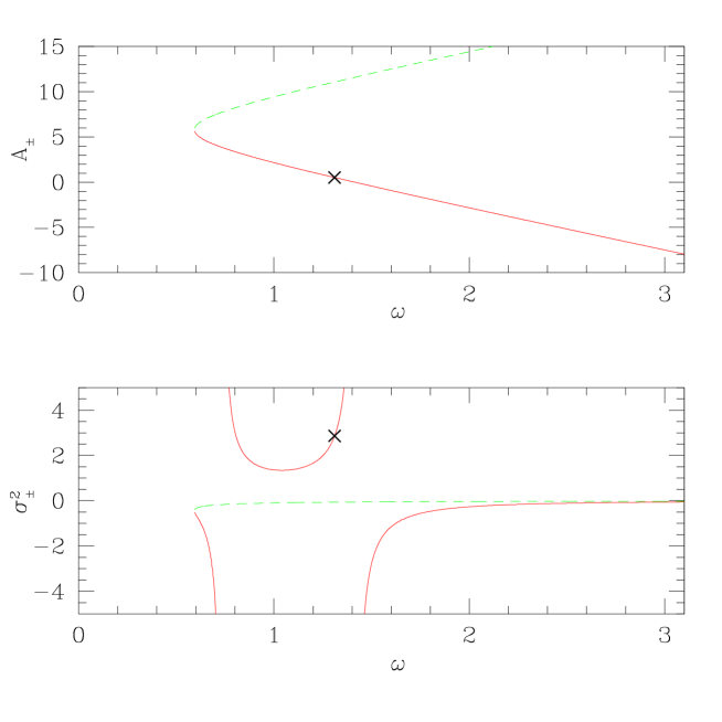
Figure 6.4: Plot of $A_{\pm}$ (top) and $\sigma^{2}_{\pm}$ (bottom) as a function of $\omega$ for hyperbolic secant $f(r/\sigma)$. The “+” roots are plotted in dashed green, while the “–” roots are plotted in solid red. The solution is not plotted for $\omega<0.595$ as the discriminant in equation (6.19) is negative and only real $A$ are of interest. The “+” roots are all unphysical since $\sigma^{2}_{+}$ is less than zero everywhere, which means that solutions within this region have an imaginary width. The solution for $\sigma^{2}_{-}$ is also unphysical outside the region $0.73<\omega<1.41$ for the same reason. Fortunately, there are solutions that are both physical (real roots) and similar to those seen in the dynamic simulations (near the x’s).

6.2.3 Hyperbolic Secant (Squared) Trial Functions

Lastly, in this subsection the field configuration is assumed to have a hyperbolic secant squared shape,

$${f\left(\frac{r}{\sigma}\right)={\rm sech}^{2}\left(\frac{r}{\sigma}\right)}.$$ (6.25)

With the new choice of $f(r/\sigma)$, the integrals (6.16) are now reevaluated:

$$\begin{array}[]{rclcrcl}\vbox{\vspace{0.75cm}}c_{1}&=&\displaystyle{\frac{2}{45}\pi^{2}}&\hbox{\hskip 28.45274pt}&c_{2}&=&\displaystyle{\frac{1}{18}\pi^{2}-\frac{1}{3}}\\ \vbox{\vspace{0.75cm}}c_{3}&=&0.1053157513&&c_{4}&=&\displaystyle{\frac{4}{105}\pi^{2}-\frac{14}{45}}.\end{array}$$ (6.26)

Using equations (6.19) and (6.20), the new $A_{\pm}$ and $\sigma^{2}_{\pm}$ are plotted as a function of $\omega$ (figure 6.5). Complex solutions exist for $\omega<0.530$ where the discriminant in (6.19) is negative. The ${\rm sech}^{2}$ function also yields unphysical solutions for all of the “–” roots since $\sigma^{2}_{-}$ is negative everywhere. Again, there is a part of the “+” solution ($0.69<\omega<1.41$) that has positive $\sigma^{2}_{+}$ and can therefore support physical solutions. Table 6.3 compares sample solutions (located near the x’s in figure 6.5) to estimates obtained from the dynamic solution.

Dynamic Parameter Solution $A_{+}=A_{D}$ $\sigma_{+}=\sigma_{D}$ $A$ 0.62 0.62 0.36 $\sigma$ 3.4 2.5 3.4 $\omega$ 1.4 1.28 1.34

Table 6.3: Table of free parameter values ($A$, $\sigma$, and $\omega$) determined using a ${\rm sech}^{2}$ trial function (third and fourth columns) compared to the values estimated from the spherically symmetric dynamics (second column); the ${\rm D}$ subscript indicates the value was obtained from the dynamic solution. The third column contains results obtained using the trial function approach where $A_{+}$ equals the amplitude of the $n=1$ mode dynamic solution; the fourth column contains results where $\sigma_{+}$ equals the width of the $n=1$ mode dynamic solution. The data from the third and fourth columns occur around the x’s in figure 6.5.

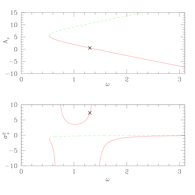
Figure 6.5: Plot of $A_{\pm}$ (top) and $\sigma^{2}_{\pm}$ (bottom) as a function of $\omega$ for hyperbolic secant squared $f(r/\sigma)$. The “+” roots are plotted in dashed green, while the “–” roots are plotted in solid red. The solution is not plotted for $\omega<0.530$ as the discriminant in equation (6.19) is negative and only real $A$ are of interest. The “+” roots are all unphysical since $\sigma^{2}_{+}$ is less than zero everywhere, which means that solutions within this region have an imaginary width. The solution for $\sigma^{2}_{-}$ is also unphysical outside the region $0.69<\omega<1.41$ for the same reason. Fortunately, there are solutions that are both physical (real roots) and similar to those seen in the dynamic simulations (near the x’s).

Chapter 7 Conclusions and Future Work

Despite its simple appearance and long history, the real scalar field keeps revealing useful and fascinating physics to those who continue to explore it. Scalar field theory (both classical and quantum) is being used throughout the frontiers of physics; although this work stresses its application to cosmology, the phenomenology discussed is widely applicable to the general theory of phase transitions.

Although oscillons had been discovered in 1977 [7],[6], and analyzed in slightly more detail in 1995 [24], the limitations in computation and numerical methods available to both research teams prevented thorough exploration. This work presents a new technique to absorb outgoing radiation in a stable and non-reflecting manner that works well for massive fields. This numerical method allows for the equations of motion to be evolved on a (relatively) small static lattice, making evolutions that previously required computational resources proportional to the square of the oscillon lifetime need only computational resources directly proportional to the oscillon lifetime. This efficiency is achieved with the combination of solving the system of equations in MIB coordinates while including higher order dissipation. In MIB cooridinates outgoing (and ingoing) characteristic velocities go to zero near the outer edge of the computational domain so the outgoing waves are compressed to nearly the Nyquist limit on the lattice where they are then quenched by dissipation. The technique proves to be stable and free of contamination in both one and two dimensional problems.

Following the more recent work of Copeland et al. [24], but with the aid of this new numerical method, this work reveals many new properties of oscillons (discussed in chapter 4). In spherical symmetry and using the symmetric double-well potential, the method was integral to the discovery of a new resonant phenomenon. Given the long lifetimes of oscillons (particularly resonant oscillons) the MIB coordinate evolutions are as much as one hundred times more computationally efficient than those previously employed. The resonances display a time scaling law and reveal (on the threshold of successive shape mode modulations) a new type of non-radiative oscillon solution. This solution’s existence and form is verified by solving a system of ordinary differential equations obtained from a periodic non-radiative ansatz. The method is also used to explore the threshold of expanding bubble formation for bubble collapse with an asymmetric double-well potential. A time scaling law is shown to exist with a scaling exponent, $\gamma\approx 2.1$.

Chapter 5 discusses the use of MIB coordinates in two dimensional axisymmetric bubble collisions. Evolutions are observed that result in expanding true-vacuum bubble formation, annihilation, coalescence, or soliton-like transmission. By looking at a two dimensional parameter space, (collision) boost velocity versus bubble width, the threshold of expanding bubble formation is again explored. The threshold reveals a time scaling law with a scaling exponent ($\gamma\approx 2.2$) similar to the spherically symmetric collapse ($\gamma\approx 2.1$). This scaling law appears to be universal in that the scaling exponents observed are independent both of the values of the critical parameters ($\sigma^{*}_{r}$ and $v^{*}_{b}$) and which parameter is varied to explore the threshold (ie. $T=\gamma\ln|p-p^{*}|$ for $p$ equal to $\sigma$ or $v_{B}$). The similarity between the scaling parameters of the spherically symmetric collapse and the axisymmetric collisions suggests that the dominant unstable mode (responsible for the critical phenomena observed) in the axisymmetric collisions might be spherically symmetric. In addition to more critical phenomena, the parameter space surveys reveal that there are many collision-induced expanding bubbles. In other words, there are many bubble configurations that would otherwise have formed oscillons and eventually dispersed, but when colliding with other bubbles combine to form an expanding vacuum bubble. In a system where bubble collisions might be occurring, nucleation rates for expanding bubbles will be higher than those originally believed to arise solely from thermal (or quantum) fluctuations.

Chapter 6 discusses oscillon solutions obtained using trial function methods. Judicious choices for trial functions allow the complete integration of the action; resulting in a system of algebraic equations instead of differential equations. Although the solutions obtained are not solutions to the true equations of motion, the predicted values for the amplitude, frequency, and width of the resonant oscillons are in reasonable agreement with observation. Furthermore, since the non-radiative resonant solution discussed in chapter 4 was not known before this work, the mere existence of the non-radiative oscillon solution obtained in such a straightforward manner was exciting.

Although there is certainly more to be discovered within the nonlinear Klein-Gordon equation, it would be interesting to see if similar physics can be found in other models. It would be interesting to see how the stability of the oscillon solutions are affected by the coupling to gravity (GR). The extra gravitational attraction might make oscillons more stable, however, the extra nonlinearities introduced might have entirely the opposite effect. It would also be interesting to see if similar phenomena are observable in the charged scalar field, both alone and coupled to electromagnetism (the charged scalar field with a SDWP coupled to electromagnetism is a simple model of superconductivity). Lastly, the numerical methods used here might be applicable to the solution of other nonlinear partial differential equations.

Chapter A Will Cosmological Oscillons Form Black Holes?

One of the most interesting applications of oscillons is to cosmological phase transitions resulting from spontaneously broken gauge symmetries. But whenever one discusses the dynamics of massive objects in a cosmological context, two questions naturally arise: How large are these objects? and How dense are these objects?. If the object is cosmologically large, then gravitational effects might need to be included since the expansion of the universe is measurable on the length-scale of the object being studied. If the object is very dense, then there will be gravitational self-interaction that will likely change the dynamics of the system. This appendix answers these two questions and shows that oscillons do not need to be modeled with general relativistic effects included.

The first thing to remember in this calculation is that (in contradiction to most relativist’s conventions), this thesis uses typical high energy physics units where $\hbar=c=1$, which implies that energy can be treated as the fundamental dimension:

$$[{\rm Energy}]=[{\rm Mass}]=[{\rm Length}]^{-1}=[{\rm Time}]^{-1}$$ (A.1)

Two useful conversion factors are $1GeV=1.7827\times 10^{-24}g$ and $1GeV^{-1}=1.9733\times 10^{-14}cm$.

This thesis almost exclusively uses dimensionless units, obtained by taking $r=\rho\,m_{H}$, $t=\tau\,m_{H}$, and $\displaystyle{\phi=\frac{\sqrt{\lambda}}{m_{H}}\,\psi}$, where $m_{H}$ is the mass in the model (the Higgs mass) and $\rho$, $t$, and $\psi$ are the dimensionful length, time, and scalar field, respectively. Converting back to dimensionful quantities, the typical oscillon radius and mass/energy are $r\approx 2.5m_{H}^{-1}$ and $\displaystyle{M\approx 43\frac{m_{H}}{\lambda}}$, respectively. Assuming the Higgs mass is known in GeV, converting the oscillon radius radius to $cm$ is performed by

$$\begin{array}[]{rcl}r&=&2.5m_{H}^{-1}\\ &=&\displaystyle{\left(\frac{2.5}{m_{H}}\right)\left(\frac{1.97\times 10^{-14}GeV\,cm}{1}\right)}\\ &=&\displaystyle{\left(\frac{4.93\times 10^{-14}GeV\,cm}{m_{H}}\right)},\end{array}$$ (A.2)

so that for an “electroweak” oscillon where the Higgs mass is $m_{H}\approx 100GeV$, $r\approx 4.93\times 10^{-16}cm$, or for a GUT oscillon with $m_{H}\approx 10^{15}GeV$, $r\approx 4.93\times 10^{-29}cm$. It is clear that these are not cosmological in their size, but what about their densities?

Since these “particles” are so small, it might be inappropriate to even consider their classical gravitational Schwarzchild radius, but for an oscillon with $M=43m_{H}$ (taking $\lambda=1$), the electroweak oscillons have $M\approx 8\times 10^{-21}g$ while a GUT oscillon would have $M\approx 8\times 10^{-8}g$. These oscillons then would have Schwarzchild radii of $\displaystyle{r_{S}=1.13\times 10^{-50}cm\,\left(\frac{m_{H}}{GeV}\right)}$, or $r_{S}\approx 10^{-48}cm$ and $r_{S}\approx 10^{-35}cm$, respectively.

So, although we do not know exactly how to describe all the forces of nature acting together at GUT energy scales, the point to be made here is that if the nonlinear Klein-Gordon action is minimally coupled to gravity, oscillons do not have a radius comparable to their Schwarzchild radius until the Higgs mass approaches $m_{H}\approx 10^{18}GeV$.

Oscillons Formula Attribute (Dependence on $m_{H}$) Radius $\displaystyle{r=4.9\times 10^{-14}cm\left(\frac{GeV}{m_{H}}\right)}$ Lifetime $\displaystyle{T=3.3\times 10^{-21}s\left(\frac{GeV}{m_{H}}\right)}$ Mass $\displaystyle{M=7.7\times 10^{-23}g\left(\frac{m_{H}}{GeV}\right)}$ Schwarzschild Radius $\displaystyle{r_{S}=1.1\times 10^{-50}cm\,\left(\frac{m_{H}}{GeV}\right)}$

Table A.1: Table displaying how to determine typical oscillon attributes them as a function of the Higgs mass. The formulae were derived using typical values (in the dimensionless coordinates used throughout this thesis) of $r=2.5$, $T=5000$, and $M=43$, for the oscillon radius, lifetime, and mass, respectively.

Ethan Philip Honda was born in Chicago, IL on December 16, 1974, the son of Sheila and Edward Honda. After completing high school at the Illinois Math and Science Academy, Aurora, IL, in 1992 he entered Loyola University Chicago as a freshman. He transfered to MIT during the fall of 1993 and received a S.B. in physics in 1996. In the fall of 1996, he entered the graduate school at the University of Texas at Austin, where he began studying numerical relativity under the supervision of Matthew Choptuik. As an adjunct faculty member from 1997 to 2000, he lectured introductory physics classes at Austin Community College. While in graduate school he was engaged to Patricia Eileen Stafford, who he will be marrying in the spring of 2001. After graduating he will be working as a postdoctoral fellow with the Signal Physics Group at the Applied Research Laboratories in Austin.

Permanent Address: 7507 N. Lowell Ave. Skokie, IL 60076 USA

This dissertation was typeset with LaTeX 2ε by the author.

Bibliography

- [1] P. Anninos, S. Oliveira, and R.A. Matzner, Phys. Rev. D 44, 1147 (1991).
- [2] R. Arnowitt, S. Deser, and C.W. Misner, “The dynamics of general relativity”, Gravitation: An introduction to current research, edited by L. Witten (John Wiley, New York, 1962).
- [3] J. Balakrishna, E. Seidel, and W-M. Suen, Phys. Rev. D D58, 104004 (1998).
- [4] N.T. Bishop, R. Gomez, P.R. Holvorcem, R.A. Matzner, P. Papadopoulos, and J. Winicour, Phys. Rev. Lett. 76, 4303-4306 (1996).
- [5] N.T. Bishop, R. Gomez,L. Lehner, M. Maharaj, and J. Winicour, Phys. Rev. D 60, 024005 (1999).
- [6] I.L. Bogolyugskii, and V.G. Makhan’kov, JETP Letters 24, 12 (1976).
- [7] I.L. Bogolyugskii, and V.G. Makhan’kov, JETP Letters 25, 107 (1977).
- [8] P.R. Brady, C.M. Chambers, and S.M.C.V. Goncalves, Phys. Rev. D 56, 6057–6061 (1997).
- [9] P.R. Brady and M.J. Cai, “Critical phenomena in gravitational collapse”, Proceedings of 8th Marcel Grossman Conference (World Scientific, Singapore).
- [10] D.K. Campbell, J.F. Schonfeld, and Charles A. Wingate, Physica 9D, 1-32 (1983).
- [11] C.M. Chambers, P.R. Brady, and S.M.C.V. Goncalves, “A Critical Look At Massive Scalar Field Collapse” Proceedings of 8th Marcel Grossman Conference (World Scientific, Singapore).
- [12] M.W. Choptuik, Ph.D. Dissertation, The University of British Columbia, 1986.
- [13] M.W. Choptuik, Phys. Rev. D 44, 3124–3135 (1991).
- [14] M.W. Choptuik, Phys. Rev. Lett. 70, 9–12 (1993).
- [15] M.W.Choptuik, T. Chmaj, and P. Bizon, Phys. Rev. Lett. 77, 424 (1996).
- [16] M.W. Choptuik, “The 3+1 Einstein equations”, unpublished (1998).
- [17] M.W. Choptuik, “Finite Difference Methods”, lecture notes, (1998).
- [18] M.W. Choptuik, gr-gc/9803075 (1998).
- [19] M.W. Choptuik, “Lectures for Taller de Verano 1999 de FENOMEC” lecture notes, (1999).
- [20] M.W. Choptuik, personal communication (2000).
- [21] S. Coleman, Phys. Rev. D 15, 2929–2936 (1977).
- [22] S. Coleman, Aspects of symmetry: selected Erice lectures of Sidney Coleman (Cambridge University Press, Cambridge, 1985).
- [23] E.J. Copeland, E.W. Kolb, and K. Lee, Nucl. Phys. B B319, 501–510 (1989).
- [24] E.J. Copeland, M. Gleiser, and H.R. Müller, Phys. Rev. D 52, 1920–1932 (1995).
- [25] R. Courant and d. Hilbert, Methods of Mathematical Physics Volume II (Wiley and Sons, New York, 1962).
- [26] G.H. Derrick, J Math. Phys. 5, 1252–1254 (1964).
- [27] A.L. Fetter and J.D.Walecka, Quantum Theory of Many-Particle Systems (McGraw-Hill, New York, 1971).
- [28] J. Frauendiener, Phys. Rev. D 58, 064002 (1998).
- [29] J. Frauendiener, Phys. Rev. D 58, 064003 (1998).
- [30] J. Frauendiener, Class. Quantum Grav. 17, 373-387 (2000).
- [31] R. Friedberg, T.D. Lee, and A. Sirlin, Phys. Rev. D 13, 2739–2761 (1976).
- [32] R. Friedberg, T.D. Lee, and Y. Pang, Phys. Rev. D 35, 3658–3677 (1987).
- [33] J. Frieman, A.V. Olinto, M. Gleiser, and C. Alcock, Phys. Rev. D 40, 3241–3251 (1989).
- [34] H. Friedrich, “15th International Conference on General Relativity and Gravitation (GR15) Proceedings” (1997).
- [35] G. Gelmini and M. Gleiser, Nucl. Phys. B B419 129–146 (1994).
- [36] V.N. Ginzburg and L.D. Landau, Zh. Exsp. Teor. Fiz 20 20, 1064 (1950).
- [37] M. Gleiser, E.W. Kolb, and R. Watkins, Nucl. Phys. B B364, 411–450 (1991).
- [38] M. Gleiser, R. Haas, Phys. Rev. D 54, 1626–1632 (1996).
- [39] M. Gleiser and A. Sornborger, patt-sol/9909002 (1999).
- [40] R. Gomez, J. Winicour, and R. Isaacson, J. Comput. Phys. 98, 11–25 (1992).
- [41] R. Gomez, P. Papdopoulos, and J. Winicour, J Math. Phys. 35, 4184–4204 (1994).
- [42] D.J. Griffiths, Introduction to elementary particles (Harper & Row, New York, 1987).
- [43] S.W. Hawking and G. Ellis, The Large Scale Structure of Space-Time, Cambridge University Press, Cambridge, 1973.
- [44] P. Hübner, Phys. Rev. D 53, 701–721 (1996).
- [45] D.A. Kirzhnits and A.D. Linde, Phys. Rev. Lett. 42B, 471 (1972).
- [46] J.A. Krumhansl and J.R. Schrieffer, Phys. Rev. B 11, 3535 (1975).
- [47] E.W. Kolb and M.S. Turner, The early universe (Addison-Wesley, Reading, MA, 1990).
- [48] H.O. Kreiss and J. Oliger, Methods for the approximate solution of time-dependent problems, GARP Publication Series No. 10 (World Meteorological Organization, Geneva, 1973).
- [49] T.D. Lee and G.C. Wick, Phys. Rev. D 9, 2291–2316 (1974).
- [50] T.D. Lee, Particle Physics and introduction to field theory (Harwood Academic Publishers, New York, 1981).
- [51] L. Lehner, personal communication (2000).
- [52] A.D. Linde, JETP Lett. 19, 320 (1974).
- [53] R.L. Marsa and M.W. Choptuik, Phys. Rev. D 54, 4929–4943 (1996).
- [54] R.A. Matzner and E. Bonning, personal communication (2000).
- [55] C.W. Misner, K.S. Thorne, and J.A. Wheeler, Gravitation (W.H. Freeman, San Francisco, 1973).
- [56] P.J. Morrison, personal communication (2000).
- [57] R. Penrose, Phys. Rev. Lett. 10, 66 (1963).
- [58] R. Rajaraman, Solitons and instantons (North-Holland Pub. Co., Amsterdam, 1982).
- [59] L.F. Richardson, Phil. Trans. Roy. Soc. 210, 307–357 (1910).
- [60] A. Riotto, Phys. Lett. B365, 64 (1996).
- [61] L.H. Ryder, Quantum Field Theory (Cambridge University Press, Cambridge, 1996).
- [62] E. Seidel and W-M. Suen, Phys. Rev. Lett. 57, 2485 (1986).
- [63] E. Seidel and W-M. Suen, Phys. Rev. Lett. 66, 1659 (1991).
- [64] J.W. Thomas, Numerical Partial Differential Equations: Finite Difference Methods (Spinger–Verlag, New York, 1995).
- [65] O.M. Umurhan, L. Tao, and E.A. Spiegel, “Stellar Oscillons”, astro-ph/9806209 (1998).
- [66] R. Wald, General Relativity (The University of Chicago Press, Chicago, 1984).
- [67] S. Weinberg, Phys. Rev. Lett. 19, 1264 (1967).
- [68] S. Weinberg, Gravitation and cosmology: Principles and applications of the general theory of relativity (John Wiley & Sons, New York, 1972).
- [69] J. Winicour, J Math. Phys. 29, 2117–2121 (1988).
- [70] J. Winicour, personal communication (1999).
Vita