Renormalization Group Flow Equations and the Phase Transition in $O(N)$–models

Abstract

We derive and solve flow equations for a general $O(N)$-symmetric effective potential including wavefunction renormalization corrections combined with a heat-kernel regularization. We investigate the model at finite temperature and study the nature of the phase transition in detail. Beta functions, fixed points and critical exponents $\beta$, $\nu$, $\delta$ and $\eta$ for various $N$ are independently calculated which allow for a verification of universal scaling relations.

1 Introduction

The manifestation of universality of critical phenomena enables the applicability of the massless $O(N)$ scalar field theories to a wide class of very different physical systems in the vicinity of the critical temperature $T_{c}$. E.g. for $N=4$ this theory is used as an effective model (the linear $\sigma$-model) for the chiral phase transition in two light-quark flavor QCD which may have the same universality class [1]. On the other hand in condensed matter physics the case $N=3$ corresponds to the well-known Heisenberg model describing the ferromagnetic phase transition. Further applications (like the Kosterlitz-Thouless phase transition ($N=2$), liquid-vapor transition describable by the continuous spin Ising model ($N=1$) or even the statistical properties of long polymer chains ($N=0$)) are often discussed in the literature.

In the vicinity of a second-order phase transition the equation of state (EoS) obeys a universal scaling form, which cannot be assessed by ordinary perturbation theory due to infrared divergences. For a negative mass term the $N$-component $\Phi^{4}$ theory exhibits spontaneous symmetry breaking of the $O(N)$-group down to $O(N-1)$ which is restored at sufficiently high temperature. According to the Goldstone-theorem ($N-1$) fields (the pions) become massless in the chiral limit and the remaining one (the radial sigma mode) stays massive. Due to these massless modes a naive perturbation expansion for the effective potential fails to give an appropriate description and the potential itself develops an imaginary part around the origin. By means of a nonperturbative Wilsonian renormalization group approach one can circumvent these difficulties and go beyond any finite order in perturbation theory.

In this work we present a renormalization group (RG) approach formulated in the Euclidean space. It is combined with a heat-kernel regularization which allows a straightforward calculation of the effective potential with an $O(N)$-symmetry for arbitrary $N$, not only at finite temperature but also directly at the critical temperature. We determine several critical exponents and investigate the phase transition regime in detail going beyond the so-called ’local potential approximation’ to also include wavefunction renormalization corrections.

The paper is organized as follows: in Sect. 2 we summarize the Wilsonian renormalization group concept and show how flow equations combined with a proper-time (heat-kernel) regularization are obtained for a general $O(N)$-symmetric potential. Based on a perturbative one-loop effective potential expression we derive flow equations for the potential and wavefunction renormalization for a $d$-dimensional massless $O(N)$ scalar theory. These coupled RG flow equations are further improved by taking into account the continuous feedbacks from the higher modes to the lower ones. The derivation of the flow equations with wavefunction renormalization corrections is given in Sect. 3.

Sect. 4 details the numerical results of the solution of the flow equations. We start with a discussion of the numerical implementation of the properly rescaled equations for a general potential with $O(N)$-symmetry on a grid whereby the full potential is numerically taken into account without resorting to polynomial approximations. The order parameter and the potential itself are studied at finite temperature.

Sect. 5 is dedicated to the critical behavior of the system at the transition temperature. The scaling solution, fixed points and beta functions are investigated in detail and numerical calculations of the critical exponents for different $N$ including the anomalous dimensions are presented. They are found to be in perfect agreement with other works and approaches. Sect. 6 contains the summary and concludes our discussion. Technical details are relegated to the appendix in order to improve the readability.

2 Concept of the RG method

The effective action $\Gamma[\Phi]$ is defined by a Legendre transformation of the generating functional $W[J]$, which generates all connected Feynman diagrams and can be expressed by a functional path integral. Except for numerical simulations, these integrals usually cannot be calculated exactly. In addition they are plagued by infrared (IR) divergences. Instead of performing the integration in one step one can follow the idea by Wilson and Kadanoff [2] and split the field $\Phi$ into fast-fluctuating and slowly-varying modes

$$\Phi(x)=\left.\Phi_{\mbox{\small slow}}(x)\right|_{q\leq k}+\left.\Phi_{\mbox{\small fast}}(x)\right|_{q\geq k}$$ (1)

and perform the functional integration only over the fast-fluctuating components with momenta $q$ larger than the scale $k$ separating both field modes from each other. The irrelevant short-distance modes which are insensitive to the physics at large correlation scales are thus eliminated. One is left with a low-energy “effective action” parameterized by the averaged fields at the IR scale $k$ which acts as a momentum cutoff. The full effective action describing the one-particle-irreducible (1PI) propagators and vertex functions is generated by the renormalized effective action in the limit $k\to 0$. Thus the $k$-dependent action provides a smooth interpolation between the bare (classical) action at an arbitrary ultraviolet (UV) scale $\Lambda$ where no quantum fluctuations are taken into account and the renormalized action in the IR. For further details we refer the interested reader to refs. [3], [4], [5], [6].

The effective action is characterized by infinitely many couplings multiplying all possible invariants which are consistent with the symmetries of theory in question. In order to proceed one has to make approximations. One possibility is the expansion of the effective action in powers of the fields about an arbitrary field $\Phi_{0}(x)$. The Taylor coefficients of this expansion $\Gamma^{(n)}(x_{1},\ldots,x_{n})$ then represent the full 1PI propagators and vertices.

Alternatively one can expand the effective action in powers of derivatives corresponding to an expansion in powers of the momenta which we will pursue in this work. The invariants are in this case classified by the number of the appearing derivatives and the coefficients are functions of constant fields. For a one-component scalar theory in $d$-dimensional coordinate space this expansion takes the form

$$\Gamma[\Phi_{c}]=\int d^{d}x\left\{-V(\Phi_{c})+\frac{1}{2}Z\left(\Phi_{c}^{2}\right)\left(\partial_{\mu}\Phi_{c}\right)^{2}+Y(\Phi_{c}^{2})\left(\left(\partial_{\mu}\Phi_{c}\right)^{2}\right)^{2}+...\right\}\ .$$ (2)

The lowest-order term, the effective potential $V$, should be a convex function, with no dependence on derivatives and can be rewritten as a sum of all 1PI Green functions $\Gamma^{(n)}$ with $n$ external lines carrying zero momenta. In other words the effective potential is the generating functional of the zero-momentum 1PI Green functions. In the following the expansion (2) will be truncated at second order ${\cal O}(\partial^{4})$ to derive a set of coupled partial differential equations for the effective potential $V$ and wavefunction renormalization $Z$ at the scale $k$.

3 Application to the $O(N)$-model

In this section the RG method will be applied to the $O(N)$-symmetric linear sigma model. We concentrate on the meson fields ($N-1$ massless pions and one massive radial sigma mode) and work with an arbitrary $N$ instead of $N=4$ fixed.

We employ the Euclidean metric due to the heat-kernel regularization for the real part of the functional determinant. This metric also allows for a straightforward extension to finite temperature within the imaginary time formalism as discussed in Section 3.3 .

At the scale $\Lambda$ in the ultraviolet region of the theory we define the effective Lagrangian for the $O(N)$-model by

$${\cal L}_{\Lambda}=\frac{1}{2}\left(\partial_{\mu}\vec{\Phi}\right)^{2}+V(\vec{\Phi}^{2})\ ;\qquad V(\vec{\Phi}^{2})=\frac{\lambda}{4}\left(\vec{\Phi}^{2}-\Phi_{0}^{2}\right)^{2}$$ (3)

with the $N$-component vector $\vec{\Phi}=(\Phi_{1},\Phi_{2},\ldots,\Phi_{N})$. The negative sign in the potential $V$ signals the broken phase and a positive sign indicates the symmetric phase.

The field $\Phi_{0}$ denotes the minimum of the potential. If this field is constant only the lowest-order term (the effective potential) of the derivative expansion of the effective action Eq. (2) can be computed. In the literature this approximation is called the ’local potential approximation’.

Higher-order terms of the derivative expansion can be calculated with a varying $x$-dependent background field $\Phi_{0}(x)$ (see e.g. [9], [10], [11]). The expansion of the effective action of the $O(N)$-symmetric model up to order ${\cal O}(\partial^{4})$ reads

$$\Gamma[\vec{\Phi}]=\int d^{d}x\left\{-V(\vec{\Phi}^{2})+\frac{1}{2}Z_{1}\left(\vec{\Phi}^{2}\right)\left(\partial_{\mu}\vec{\Phi}\right)^{2}+\frac{1}{2}Z_{2}\left(\vec{\Phi}^{2}\right)\left(\vec{\Phi}\partial_{\mu}\vec{\Phi}\right)^{2}\right\}\ .$$ (4)

To this order there are two independent wavefunction renormalization terms $Z_{1}$ and $Z_{2}$ for $N>1$ .

In the following we will sketch the derivation of the flow equation including the wavefunction renormalization corrections. The perturbative one-loop contribution to the effective action yields formally a non-local logarithm which must be regularized. Proper-time regularization is the most commonly used regularization for the real part of the determinant and results in a finite local action (see e.g. [12]). It was introduced by Schwinger and maintains a finite sharp dimensionful proper-time cutoff [13]. We replace this sharp ultraviolet cutoff for the proper-time variable $\tau$ by a smooth, $a$ $priori$ unknown, kernel or ’blocking function’ $f_{k}$ in the integrand which will be specified later.

After introducing a complete set of plane wave states in the heat kernel [14] this results in the following $d$-dimensional effective action

$$\Gamma[\vec{\Phi}]=-\frac{1}{2}\int d^{d}x\int_{0}^{\infty}\frac{d\tau}{\tau}f_{k}\int\frac{d^{d}p}{(2\pi)^{d}}\mbox{tr}\ e^{-\tau\left(p^{2}-2ip_{\mu}\partial_{\mu}-\partial^{2}+V_{ij}^{\prime\prime}(\Phi)\right)}$$ (5)

with the shorthand notation $V_{ij}^{\prime\prime}(\Phi)=\frac{\delta^{2}V}{\delta\Phi_{i}\Phi_{j}}$ for the $(N\times N)$-matrix valued second derivative of the $O(N)$-symmetric potential $V$ given by

$$V_{ij}^{\prime\prime}=\lambda\left(\vec{\Phi}^{2}-\Phi_{0}^{2}\right)\delta_{ij}+2\lambda\Phi_{i}\Phi_{j}\ .$$ (6)

The trace in Eq. (5) runs over the $N$ fields and can be computed analytically with standard techniques [15], [16]. In the following we omit the index structure of the potential term $V_{ij}^{\prime\prime}$ and follow the techniques outlined in ref. [17] which we generalize to an $O(N)$-symmetric matrix-valued potential $V^{\prime\prime}$.

The expansion of $\exp\left[-\tau\left(-2ip_{\mu}\partial_{\mu}-\partial^{2}+V^{\prime\prime}\right)\right]$ in Eq. (5) in powers of derivatives up to second order yields

$$\Gamma_{2} = -\frac{1}{2}\int\!\!d^{d}x\!\int\!\frac{d\tau}{\tau}f_{k}\int\frac{d^{d}p}{(2\pi)^{d}}e^{-\tau p^{2}}$$ (7)

$$\cdot\mbox{tr}\left\{\sum_{n=0}^{\infty}(-1)^{n}\frac{\left(V^{\prime\prime}\right)^{n}\tau^{n}}{n!}+\sum_{n=2}^{\infty}\frac{(-1)^{n-1}\tau^{n}}{n!}\sum_{k=0}^{n-1}\left(V^{\prime\prime}\right)^{k}\partial^{2}\left(V^{\prime\prime}\right)^{n-1-k}\right.$$

$$\left.\ \ \ -4p_{\mu}p_{\nu}\sum_{n=3}^{\infty}\frac{(-1)^{n-1}\tau^{n}}{n!}\sum_{k=0}^{n-2}\left(V^{\prime\prime}\right)^{k}\partial_{\mu}\sum_{l=0}^{n-2-k}\left(V^{\prime\prime}\right)^{l}\partial_{\nu}\left(V^{\prime\prime}\right)^{n-2-l-k}\right\}\ \ \ \$$

where all linear terms in the momenta $p_{\mu}$ are ignored since they vanish anyhow after odd $p$-integration. The above expression can be further simplified by a tedious but straightforward calculation . All infinite sums converge and can be evaluated analytically with careful attention of the non-commuting operator order.

To improve readability we will use in the following the abbreviations

$$m^{2}_{\sigma}\equiv\lambda(3\vec{\Phi}^{2}-\Phi_{0}^{2})\quad\mbox{and}\quad m^{2}_{\pi}\equiv\lambda(\vec{\Phi}^{2}-\Phi_{0}^{2})$$ (8)

and exploit the $O(d)$ symmetry of the momentum integration.

To order ${\cal O}(\partial^{4})$ the effective action splits into two parts:

$$\Gamma_{2}=\Gamma^{(0)}+\Gamma^{(2)}$$

with $\Gamma^{(0)}$ denoting the one-loop potential contribution (no derivatives)

$$\Gamma^{(0)}=-\frac{1}{2}\int d^{d}x\int\frac{d\tau}{\tau}f^{(0)}_{k}\int\frac{d^{d}p}{(2\pi)^{d}}e^{-\tau p^{2}}\left\{e^{-\tau m_{\sigma}^{2}}+(N-1)e^{-\tau m_{\pi}^{2}}\right\}$$ (9)

and $\Gamma^{(2)}$ the second-order contribution (containing two derivatives)

$$\Gamma^{(2)} = \frac{1}{2}\int d^{d}x\int\frac{d\tau}{\tau}f^{(1)}_{k}\int\frac{d^{d}p}{(2\pi)^{d}}e^{-\tau p^{2}}\left\{\left(\frac{\tau^{2}}{2}\partial^{2}m_{\sigma}^{2}-\frac{\tau^{3}}{3}\partial_{\mu}m_{\sigma}^{2}\partial_{\mu}m_{\sigma}^{2}\right)e^{-\tau m_{\sigma}^{2}}\right.$$

$$\hskip 113.81102pt+(N-1)\left(\frac{\tau^{2}}{2}\partial^{2}m_{\pi}^{2}-\frac{\tau^{3}}{3}\partial_{\mu}m_{\pi}^{2}\partial_{\mu}m_{\pi}^{2}\right)e^{-\tau m_{\pi}^{2}}$$

$$\qquad\quad-2\left(\frac{2}{m_{\sigma}^{2}-m_{\pi}^{2}}\left(e^{-\tau m_{\sigma}^{2}}-e^{-\tau m_{\pi}^{2}}\right)+\tau\left(e^{-\tau m_{\sigma}^{2}}+e^{-\tau m_{\pi}^{2}}\right)\right)$$

$$\hskip 202.01474pt\left(\frac{(\Phi_{a}\partial_{\mu}\Phi_{a})^{2}}{(\vec{\Phi}^{2})^{2}}-\frac{(\partial_{\mu}\Phi_{a})^{2}}{\vec{\Phi}^{2}}\right)$$

$$-\frac{p^{2}\delta^{\mu\nu}}{d}\left[\left(\frac{2\tau^{3}}{3}\partial^{2}m_{\sigma}^{2}-\frac{\tau^{4}}{2}\partial_{\mu}m_{\sigma}^{2}\partial_{\mu}m_{\sigma}^{2}\right)e^{-\tau m_{\sigma}^{2}}\right.$$

$$\qquad\qquad+(N-1)\left(\frac{2\tau^{3}}{3}\partial^{2}m_{\pi}^{2}-\frac{\tau^{4}}{2}\partial_{\mu}m_{\pi}^{2}\partial_{\mu}m_{\pi}^{2}\right)e^{-\tau m_{\pi}^{2}}$$

$$\qquad\qquad+2\tau\left(\frac{2}{m_{\sigma}^{2}-m_{\pi}^{2}}\left(e^{-\tau m_{\sigma}^{2}}-e^{-\tau m_{\pi}^{2}}\right)+\tau\left(e^{-\tau m_{\sigma}^{2}}+e^{-\tau m_{\pi}^{2}}\right)\right)$$

$$\hskip 184.9429pt\left.\left.\left(\frac{(\partial_{\mu}{\Phi}_{a})^{2}}{\vec{\Phi}^{2}}-\frac{({\Phi}_{a}\partial_{\mu}{\Phi}_{a})^{2}}{(\vec{\Phi}^{2})^{2}}\right)\right]\right\}\ .$$

For $N=1$ this outcome for $\Gamma^{(2)}$ agrees with that obtained in ref. [17] using a similar procedure.

In order to extract the two different wavefunction renormalization $Z_{1}$ and $Z_{2}$ of the effective action $\Gamma$ in Eq. (4) one has to collect the terms in front of $(\partial_{\mu}\vec{\Phi})^{2}$ and of $(\vec{\Phi}\partial_{\mu}\vec{\Phi})^{2}$. To simplify the amount of work drastically we will use the truncation to a uniform wavefunction renormalization which means we neglect the field and momentum dependence of the wavefunction renormalization. This approximation corresponds to considering only the wavefunction renormalization constants at the minimum of the potential $\Phi_{0}$ and neglecting their derivatives.

For $N>1$ one has to work with two different $Z_{1}$ and $Z_{2}$ corresponding to two anomalous dimensions. These are related to the wavefunction renormalization for the Goldstone modes $Z_{\pi}$ and the radial mode $Z_{\sigma}$ via

$$Z_{\pi}=Z_{1}\quad\quad;\quad\quad Z_{\sigma}=Z_{1}+\vec{\Phi}^{2}Z_{2}\ .$$

As will be seen later the difference between the corresponding anomalous dimensions at the scaling solution vanishes. We can further simplify the calculation by neglecting $Z_{2}$. This approximation describes all the qualitative features at the phase transition without loss of quantitative predictive power.

Comparing the expressions in (9) and (10) with Eq. (4) we can now extract the effective potential contribution

$$V=-\frac{1}{2(4\pi)^{d/2}}\int\frac{d\tau}{\tau}\frac{1}{(Z\tau)^{d/2}}f^{(0)}_{k}\left\{e^{-\tau m_{\sigma}^{2}}+(N-1)e^{-\tau m_{\pi}^{2}}\right\}$$ (11)

and the $Z_{1}\equiv Z$ wavefunction renormalization contribution

$$Z = -\frac{1}{(4\pi)^{d/2}}\frac{Z}{\Phi_{0}^{2}}\int\frac{d\tau}{\tau}\frac{1}{(Z\tau)^{d/2}}\left[\left(f^{(1)}_{k}-2f^{(0)}_{k}\right)\right.$$

$$\qquad\qquad\left.\left\{\tau\left(e^{-\tau m_{\sigma}^{2}}+e^{-\tau m_{\pi}^{2}}\right)+\frac{2}{m^{2}_{\sigma}-m^{2}_{\pi}}\left(e^{-\tau m_{\sigma}^{2}}-e^{-\tau m_{\pi}^{2}}\right)\right\}\right]\ ,$$

where momenta have been rescaled by the corresponding wavefunction renormalization.

Note, that we have introduced two different blocking functions, $f^{(0)}_{k}$ and $f^{(1)}_{k}$ to be discussed in the next Section. To proceed we differentiate Eqs. (11), (3) with respect to the scale $k$ which is introduced via the blocking functions thus obtaining the desired flow equations for the potential and wavefunction renormalization. In doing so one has to know the derivative of the blocking functions $f^{(i)}_{k}$ $i=0,1,\ldots$ with respect to $k$.

3.1 The regulating blocking functions

In this Section we sketch the way how to implement the regulating blocking functions $f^{(i)}_{k}(\tau)$ in the proper-time integrations. They serve to cut off the diverging momentum contributions to the flow equations (see e.g. [17, 18]). Going beyond the local potential approximation by including higher contributions to the effective potential through the wavefunction renormalization we have to deal with different powers of momenta. In deriving flow equations for an $O(N)$-symmetric potential we there encounter additional momentum integrals which force us to modify the blocking functions. In fact, at each level of the gradient- or derivative expansion new blocking functions must be taken into account (cf. e.g. [18]). In order to find a condition on the structure of the blocking functions we compare the operator regularization method to a momentum regularization method. In ref. [4] a differential equation for the blocking function in the local potential approximation was found by comparing the operator cutoff to a sharp momentum cutoff. This yields RG flow equations with a characteristic logarithmic structure similar to the Wegner-Houghton equation [19]. When the momenta are rescaled as $p^{2}\to Zp^{2}$ we obtain a similar $d$-dimensional equation

$$kf_{k}^{(0)\ \prime} = -\frac{2}{\Gamma(d/2)}\left(\tau Zk^{2}\right)^{d/2}e^{-\tau Zk^{2}}\ .$$ (13)

The function $f_{k}^{(0)}$ regulates momentum integrals of the form

$$I_{0}=\int\frac{d^{d}p}{(2\pi)^{d}}e^{-\tau Zp^{2}}\ .$$ (14)

and plays a similar role as the covariant Pauli-Villars cutoff. Its derivation can be found in detail in refs. [4],[5].

The above expression must be modified when higher derivatives are taken into account because one encounters higher powers in the momentum integrals of the form e.g.

$$I_{2}=\int\frac{d^{d}p}{(2\pi)^{d}}e^{-\tau Zp^{2}}p_{\mu}p_{\nu} = \frac{\delta_{\mu\nu}}{d}\int\frac{d^{d}p}{(2\pi)^{d}}e^{-\tau Zp^{2}}p^{2}\ .$$ (15)

Comparing the sharp momentum cutoff version of $I_{2}$ with the proper-time expression with a new blocking function $f^{(1)}_{k}$ and by taking the derivative with respect to $k$ one obtains the following equation

$$kf^{(1)\ \prime} = -\frac{4}{d\Gamma(d/2)}\left(\tau Zk^{2}\right)^{d/2+1}e^{-\tau Zk^{2}}\ .$$ (16)

Thus each power of $p^{2}$ in the numerator of the integrand (cf. Eq.(15)) generates an additional power in the proper-time variable $\tau$ thereby accelerating the convergence of the flow equation. This result is identical to that in ref. [18].

For completeness we quote the result for the blocking function $f_{k}^{(2)}$ which regularizes momentum integrals of the form

$$I_{4}=\int\frac{d^{d}p}{(2\pi)^{d}}e^{-\tau Zp^{2}}p_{\mu}p_{\nu}p_{\lambda}p_{\rho}\ .$$ (17)

Although they are not needed in our approximation we will employ such higher blocking functions when we analyze the influence of the blocking functions on the convergence of the flow equations in Sect. 5.4.

Comparing $f_{k}^{(2)}$ in the same manner with a sharp cutoff version yields the differential equation

$$kf_{k}^{(2)\ \prime} = -\frac{8}{d(d+2)\Gamma(d/2)}\left(\tau Zk^{2}\right)^{d/2+2}e^{-\tau Zk^{2}}\ .$$ (18)

3.2 The flow equations

With the general differential equation for the blocking function $f^{(i)}_{k}$ at hand we can immediately obtain the flow equations. It turns out that the lowest blocking function $f^{(0)}_{k}$ is sufficient to regulate the potential equation alone (no derivatives) but not for higher momentum contributions. The convergence of the solution of the flow equation is very poor with $f^{(0)}_{k}$ when wavefunction contributions are taken into account. This result agrees with that found in [4],[5]. Thus in order to accelerate the convergence from the very beginning we chose a blocking function $f^{(i)}_{k}$ with $i>0$. We start with $i=1$ and replace in Eqs. (11),(3) $f^{(0)}_{k}$ by $f^{(1)}_{k}$. Performing now the convergent proper-time integration this yields the flow equations

$$\partial_{t}V=S_{d}\frac{k^{d}}{d}\left[\frac{1}{1+2v^{\prime}+4\Phi^{2}v^{\prime\prime}}+\frac{N-1}{1+2v^{\prime}}\right]$$ (19)

for the potential and

$$-\frac{1}{Z}\partial_{t}Z=\left.\frac{2S_{d}}{\Phi^{2}Zk^{2}}\frac{k^{d}}{d}\left[1+\frac{1}{(1+4\Phi^{2}v^{\prime\prime})^{2}}+\frac{1}{2\Phi^{2}v^{\prime\prime}}\left(\frac{1}{1+4\Phi^{2}v^{\prime\prime}}-1\right)\right]\right|_{{\Phi^{2}=\Phi_{0}^{2}}}$$ (20)

for the wavefunction renormalization where we have introduced the notations:

$$\partial_{t}V\equiv k\frac{\partial V}{\partial k}\qquad,\qquad v^{(i)}\equiv\frac{V^{(i)}}{Zk^{2}}\qquad\mbox{and}\qquad S_{d}=\frac{2}{\Gamma(d/2)(4\pi)^{d/2}}\ .$$

A prime on the potential $V$ denotes differentiation with respect to $\Phi^{2}$. Due to our uniform wavefunction renormalization approximation (no derivatives of $Z$) we have to evaluate the flow equation at the potential minimum $\Phi^{2}_{0}$. The functions in squared brackets describe the threshold behavior of massive modes and are sometimes called ’threshold functions’ [6]. Each massive mode decouples from the evolution towards the infrared limit $k\to 0$ (see details in [5]). One advantage of our choice of the blocking functions is that the threshold functions can be obtained analytically. In Eq. (19) one recognizes the persistent contribution of the ($N-1$) massless Goldstone particles to the evolution since $v^{\prime}$ vanishes for the minimum of the potential (cf also Eq. (20)).

In the above flow equations we, in addition, perform a renormalization group improvement thus going beyond the independent-mode approximation. The improvement consists of replacing the bare potential $V$ (and its derivatives) on the $rhs$ of the flow equations with the running $k$-dependent counterpart $V_{k}$. Then higher graphs such as daisy and super-daisy diagrams are taken into account. Thus we substitute

$$m_{\sigma}^{2}\equiv 2V^{\prime}_{k}+4\Phi^{2}V^{\prime\prime}_{k}\qquad\mbox{and}\qquad m_{\pi}^{2}\equiv 2V^{\prime}_{k}\ ,$$ (21)

which should not be confused with the abbreviation in Eq. (8). Of course, the potential $V_{k}$ is still a function of the field $\Phi^{2}$ itself. This type of nonlinear flow equations has to be solved numerically on a grid as discussed in the next Section.

3.3 Finite temperature

Here we wish to discuss the generalization to finite temperature. Within the Matsubara formalism this is easily accomplished by replacing the $d$-dimensional momentum integration in Eqs. (9) and (3) by a $(d-1)$–dimensional integration and by introducing a discrete Matsubara summation with bosonic frequencies $\omega_{n}=2n\pi T$ in the zero-momentum component. An additional length scale (the inverse temperature) is now introduced and besides quantum fluctuations additional thermal fluctuations appear. At finite temperature the scale $k$ serves a generalized IR cutoff for a combination of the three-dimensional momenta and discrete frequencies. The influence of the different choices of blocking functions on the two types of modes can be found in more detail in [20]. We use in this work cutoff blocking functions with a $d$-dimensional momentum variable.

In order to be consistent with the zero-temperature flow equations we make the same approximations and use the same blocking function $f_{k}^{(1)}$ at finite temperature. The finite-temperature extension of Eqs. (19) and (20) with a uniform wavefunction renormalization contribution is

$$\partial_{t}V = \frac{Tk^{3}}{8(4\pi)}\left\{{\cal M}\left(0,\frac{m^{2}_{\sigma}}{Zk^{2}},\frac{3}{2}\right)+(N-1){\cal M}\left(0,\frac{m^{2}_{\pi}}{Zk^{2}},\frac{3}{2}\right)\right\}\qquad$$ (22)

where the following abbreviations for the finite-temperature threshold functions

$${\cal M}\left(p,m^{2},\alpha\right) = \sum_{n=-\infty}^{\infty}\frac{(\omega^{2}_{n})^{p}}{(1+\omega^{2}_{n}/k^{2}+m^{2})^{\alpha}}\$$ (23)

have been introduced together with the short-hand notation of Eq. (21). For the uniform finite-temperature wavefunction flow equation we obtain accordingly

$$\partial_{t}Z = -\frac{Z}{\Phi_{0}^{2}}\frac{Tk^{3}}{(4\pi)^{3/2}}\left\{\frac{5}{2}\frac{\Gamma(3/2)}{m^{2}_{\sigma}-m^{2}_{\pi}}\left[{\cal M}\left(0,\frac{m^{2}_{\sigma}}{Zk^{2}},\frac{3}{2}\right)-{\cal M}\left(0,\frac{m^{2}_{\pi}}{Zk^{2}},\frac{3}{2}\right)\right]\right.$$ (24)

$$\qquad\qquad\qquad\left.+\frac{5}{4}\frac{\Gamma(5/2)}{Zk^{2}}\left[{\cal M}\left(0,\frac{m^{2}_{\sigma}}{Zk^{2}},\frac{5}{2}\right)+{\cal M}\left(0,\frac{m^{2}_{\pi}}{Zk^{2}},\frac{5}{2}\right)\right]\right.$$

$$\qquad\qquad\quad\left.+\frac{\Gamma(5/2)}{m^{2}_{\sigma}-m^{2}_{\pi}}\frac{1}{k^{2}}\left[{\cal M}\left(1,\frac{m^{2}_{\pi}}{Zk^{2}},\frac{5}{2}\right)-{\cal M}\left(1,\frac{m^{2}_{\sigma}}{Zk^{2}},\frac{5}{2}\right)\right]\right.$$

$$\qquad\qquad\left.-\frac{\Gamma(7/2)}{2Zk^{2}}\frac{1}{k^{2}}\left[{\cal M}\left(1,\frac{m^{2}_{\sigma}}{Zk^{2}},\frac{7}{2}\right)+{\cal M}\left(1,\frac{m^{2}_{\pi}}{Zk^{2}},\frac{7}{2}\right)\right]\right\}.$$

It is possible to calculate the zero-temperature limit of the finite-temperature flow equation (22) and (24) analytically by using the zero-temperature limit of the threshold functions:

$${\cal M}\left(0,m^{2},\alpha\right)\to\frac{k}{\pi T}\frac{2\cdot 4\cdots(2\alpha-3)}{1\cdot 3\cdots(2\alpha-2)}\frac{1}{(1+m^{2})^{(2\alpha-1)/2}}$$ (25)

and

$${\cal M}\left(1,m^{2},\alpha\right)\to\frac{k^{3}}{2\pi T}\frac{2\cdot 4\cdots(2\alpha-5)}{1\cdot 3\cdots(2\alpha-4)}\frac{1}{(\alpha-1)}\frac{1}{(1+m^{2})^{(2\alpha-3)/2}}\ .$$ (26)

In the next section we discuss the numerical solution of these equations for the broken phase.

4 Results

4.1 Numerical implementation

We discretize the field $\Phi^{2}$ for a general potential term $V(\Phi^{2})$ on a grid and numerically solve the coupled set of flow equations (19),(20) for zero temperature and (22)-(24) for finite temperature at each grid point.

The flow equations incorporate derivatives of $V$ with respect to the field $\Phi^{2}$ up to second order. Thus further differentiation of the flow equation with respect to the fields increases the order of derivatives of $V$. Following the method described in [21] we calculate the first- and second derivative of the flow equation for the potential with respect to $\Phi^{2}$ and thus generate derivatives of $V$ up to fourth order. The unknown derivatives $V^{\prime\prime\prime}$ and $V^{\prime\prime\prime\prime}$ are determined by matching conditions at intermediate grid points in order to close the highly coupled system of differential equations. This matching condition is based on a Taylor-expansion of $V^{\prime}$ and $V^{\prime\prime}$ up to forth order at each grid point $\Phi^{2}_{i}$ and it requires continuity of these expansions at intermediate adjoining grid points.

For $n$ grid points one obtains $2n-2$ equations for the $2n$ unknown derivatives $V^{\prime\prime\prime}$ and $V^{\prime\prime\prime\prime}$. The missing two conditions of the boundary grid points are determined by an expansion of the third derivatives. This results in an $2n$-dimensional algebraic coupled set of flow equations for $V^{\prime}$ and $V^{\prime\prime}$ which can be solved by a fifth-order Runge Kutta algorithm with adaptive step size [22].

With the grid algorithm described above the flow equations are solved starting the evolution in the broken phase deep in the UV region at a given $k=\Lambda$ where we use a tree-level parameterization of the potential with only two initial parameters. For the results presented below the values $\Lambda=800$ MeV, $\Phi^{2}_{0,\Lambda}=(140$ MeV$)^{2}$, $\lambda_{\Lambda}=49$ and $Z_{\Lambda}=0.8$ have been chosen.

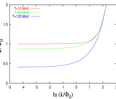
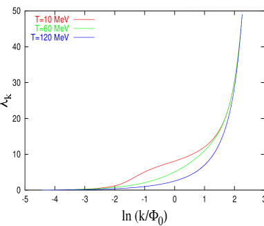
Figure 1: The $k$-evolution of the minimum of the full potential (left panel) and of the quartic coupling $\lambda_{k}$ (right panel) for various temperatures.

The evolution with respect to the scale $k$ of the dimensionful minimum of the potential $\Phi_{0,k}$ in units of $\Phi_{0}(T=0)$ and the quartic coupling $\lambda_{k}$ for $N=4$ is shown in Fig. 1 for different temperatures without wavefunction renormalization corrections. The initial values at the UV scale $\Lambda$ are fixed at $T=0$ and are kept constant for all temperatures. This, in principle, limits the predictive power of the high-temperature behavior of the calculated quantities. We have checked that for the range of temperatures relevant for the phase transition the results are insensitive to temperature variations in $\Lambda$ within reasonable limits.

For all temperatures below $T_{c}$ the minimum $\Phi_{0,k}/\Phi_{0}(T=0)$ (left panel) decreases as a function of $k$ and settles down to a constant for very small $k$-values where we can stop the evolution to obtain the renormalized vacuum expectation value ($\Phi_{0}$) (cf. [23]). Which is the physical order parameter for the $O(N)$ symmetry phase transition.

The quartic coupling $\lambda_{k}$ which in four dimensions is a dimensionless quantity shows a logarithmic running and tends to zero for $k\to 0$ as can be seen in the right panel of Fig. 1. For $N>1$ there are $(N-1)$ massless pions in the spontaneously broken phase. Below the phase transition they never decouple from the evolution and thus always contribute to the logarithmic running resulting in an infrared-free theory. The undulation in the curve for small temperature ($T=10$ MeV) is a numerical artefact and stems from the finite grid spacing.

4.2 The potential and the quark condensate

In the infrared the order parameter $\Phi_{0}$ signals a second-order phase transition (see Fig. 2).

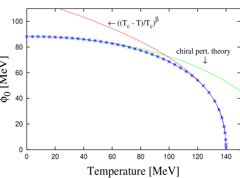
Figure 2: The order parameter for the $O(4)$-model as a function of temperature. A comparison with the chiral perturbation theory expansion for low temperatures and with the Widom scaling function in the vicinity of the critical temperature is also shown.

The vacuum expectation value is obtained as the dimensionful minimum of the full effective potential with respect to the field, including wavefunction renormalization contributions. For low temperatures we compare our result for $N=4$ with a three-loop chiral perturbation theory expansion up to order ${\cal O}\left((T/f_{\pi})^{8}\right)$ [24] and find perfect agreement up to $T\approx 45$ MeV. The critical temperature is a non-universal quantity and therefore depends on the initial UV parameters. Our value of $T_{c}\approx 140$ MeV is higher than the value $T_{c}\approx 100$ MeV of ref. [6] also obtained for a full potential analysis with the exact renormalization group including wavefunction renormalization contributions. This discrepancy in the value of $T_{c}$ might be due to the different implementations of the threshold functions in the flow equations. In the vicinity of $T_{c}$ we see a scaling behavior of the order parameter with a critical exponent $\beta\approx 0.4$ also depicted in Fig. 2.

In our analysis we are not restricted to universal quantities such as the minimum of the potential. Indeed we do know the entire potential as function of the field $\Phi$ which is shown in Fig. 3 (left panel) in the $k\to 0$ limit for various temperatures ($T=0$, $T=T_{c}$ and $T>T_{c}$). Here one again observes a second-order phase transition. Numerically we have to stop the evolution at a very small but finite $k$-value which slightly influences the final shape of the potential. In fact, the potential at $k=0$ corresponds to the free-energy density which should be a flat function around the origin due to convexity. For a finite $k$-value we always obtain the well-known Mexican hat form for the broken phase (right panel). The evolution towards the Maxwell construction ([25]) at $T=0$ can explicitly be seen.

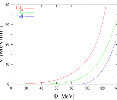
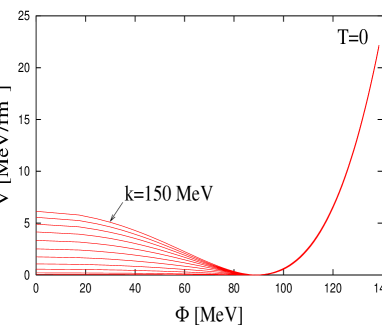
Figure 3: The dimensionful convex potential for different temperatures (left panel) and the $k$-evolution of the dimensionful potential at $T=0$ (right panel) towards zero.

5 Critical behavior

Within the RG approach we can directly link the zero-temperature physics to the universal behavior in the vicinity of the critical temperature. We will restrict ourselves to temperatures $T\leq T_{c}$ in this section but there is in general no restriction to the broken phase.

In order to investigate the critical regime of the system it turns out that the use of rescaled quantities is convenient since the scale $k$ is no longer present explicitly in the evolution equations. At the critical temperature only properly rescaled quantities asymptotically exhibit scaling and the evolution of the system is purely three-dimensional. This is the well-known dimensional reduction phenomenon (see e. g. ref. [26]) and is exhibited in the structure of the above mentioned threshold functions. It is also the reason for the fractional power in the threshold functions at finite temperature in Eqs. (22)-(24). For the dimensionally reduced system at high temperature ($T\gg k$) only the bosonic zero-mode Matsubara frequencies are important while all the other modes decouple completely from the evolution.

We define the rescaled (dimensionless) quantities as follows

$${\phi}^{2}:=k^{-(d-2+\eta)}\Phi^{2}$$ (27)

where we have introduced the anomalous dimension

$$\eta=-\frac{\partial}{\partial t}\ln Z_{k}.$$ (28)

As already mentioned in Sect. 3 there are in general two anomalous dimensions for the $O(N)$-model, one for the radial mode and another one for the Goldstone bosons. Due to our uniform wavefunction renormalization approximation we work with only one $\eta$.

In this section all results are obtained by taking the corrections due to the anomalous dimension $\eta$ explicitly into account. In order to deal with dimensionless flow equations we additionally rescale the potential via

$$u({\phi}^{2}):=k^{-d}V({\phi}^{2})\ .$$ (29)

All dimensionless quantities are denoted in the following by small letters.

From Eqs. (19)-(20) we obtain the following properly rescaled dimensionless flow equations in $d$ dimensions

$$\partial_{t}u({\phi}^{2}) = -du+(d-2+\eta){\phi}^{2}u^{\prime}+\frac{S_{d}}{d}\left[\frac{1}{1+2u^{\prime}+4{\phi}^{2}u^{\prime\prime}}+\frac{N-1}{1+2u^{\prime}}\right]\ \$$ (30)

$$-\frac{1}{Z}\partial_{t}Z = \left.\frac{2S_{d}}{{\phi}^{2}d}\left[1+\frac{1}{(1+4{\phi}^{2}u^{\prime\prime})^{2}}+\frac{1}{2{\phi}^{2}u^{\prime\prime}}\left(\frac{1}{1+4{\phi}^{2}u^{\prime\prime}}-1\right)\right]\right|_{\phi=\phi_{0}}\ ,$$ (31)

where the primes on the potential $u$ indicate differentiation with respect to ${\phi^{2}}$. Since no scale $k$ appears explicitly in the rescaled equations they are in a scale-independent form. Due to the dimensional reduction phenomenon we do not need to use the finite temperature flow equations at the critical temperature. It is sufficient to employ the three-dimensional zero-temperature equations in oder to investigate the critical regime of the phase transition.

5.1 The scaling solution and fixed points

We solve the set of coupled equations (30), (31) for arbitrary $N$ with the same initial values at $t=0$. We arbitrarily set $\lambda=0.5$ which is anyway an irrelevant quantity and finetune only $\left.{\phi_{0}^{2}}\right|_{t=0}$ at $t=0$ in order to find a $k$-independent solution, the so-called ’scaling solution’ of the flow equations. A second-order phase transition involves an infrared fixed point of the renormalization group. Therefore the physics close to the phase transition is scale invariant and the critical behavior should be described by a scale-independent solution.

For an initial value around the critical $\left.{\phi_{0}^{2}}\right|_{t=0}^{cr}$ at the UV scale $t=0$ this is indeed the case and the evolution towards the infrared $t\to-\infty$ reaches almost the scaling solution where the $t$-dependence vanishes and ${\phi_{0}^{2}}$ tends to a constant (fixed point) value ${\phi_{0}^{2}}^{*}$. This feature is demonstrated in Fig. 4 where the evolution of ${\phi_{0}^{2}}$ versus the “flow time” $t=\ln(k/\Lambda)$ is shown for different initial values at the UV scale $t=0$.

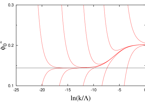
Figure 4: The evolution of the dimensionless minimum $\phi_{0}^{2}$ as function of the “flow time” $t=\ln(k/\Lambda)$ for $N=4$ and different initial values at $t=0$ around the critical value $\left.{\phi_{0}^{2}}\right|_{t=0}^{cr}$ (see text for details).

For a starting value near the critical value $\left.{\phi_{0}^{2}}\right|_{t=0}^{cr}$ the evolution deviates either towards the spontaneously broken (${\phi_{0}^{2}}\neq 0$) or the symmetric (${\phi_{0}^{2}}=0$) phase in the infrared as shown in Fig. 4. Due to the rescaling of the dimensionful minimum $\Phi_{0}^{2}$ (cf Eq. (27)) which in the infrared tends to a constant value or zero during the evolution with respect to the scale $k$, the dimensionless minimum ${\phi_{0}^{2}}=\Phi^{2}_{0}/k^{2}$ diverges for $k\to 0$ for the broken phase as can be seen in Fig. 4.

In the further course of the evolution, for a initial value very close to the critical one at $t=0$, the scaling regime is approached where the system spends a long “time” before it finally deviates from it again. The scaling solution for the minimum of the potential is denoted by a straight line in Fig. 4.

Not only ${\phi_{0}^{2}}$ but all other quantities reach the scaling solution around $t\approx-10$ and leave the critical trajectory at $t\approx-18$. The time that the system spends on this scaling solution can be rendered arbitrarily long by appropriate finetuning of the initial values at the UV cutoff scale i.e. at $t=0$. In order to produce such a high precision as shown in the Figure one has to know the initial starting value up to $13$ digits.

Besides of the trivial high-temperature and low-temperature fixed points the $O(N)$-symmetric model exhibits a nontrivial mixed fixed point inherent in the flow equations. The region around this fixed point is mapped out in Fig. 5 where the rescaled dimensionless quantities ${\phi_{0}^{2}}$ and $\lambda$ are plotted for $N=4$ and for different initial values during the evolution towards the infrared. The arrows in the Figure characterize the flow w.r.t. the scale $t$ towards zero.

In general, there are two relevant physical parameters for the $O(N)$ model which must be adjusted to bring the system to the critical fixed point according to universality class arguments. Consider for example the ferromagnetic spin Ising model with a discrete symmetry $Z_{2}=O(1)$ where the relevant parameters are the temperature and external magnetic field. Since we work in this section in the chiral limit (no external sources or masses) only one relevant eigenvalue from the linearized RG equations is left, the temperature. This can be seen in Fig. 5. The quantity ${\phi_{0}^{2}}$ is the relevant variable because repeated renormalization group iterations (which are the discrete analog to the continuous evolution with respect to $t\to-\infty$) drive the variable away from the fixed-point value while $\lambda$ is the irrelevant variable and is iterated towards the fixed point if the initial values are chosen sufficiently close to the fixed point. Thus one has a one-dimensional curve of points attracted to the fixed point, the so-called ’critical surface’ where the correlation length diverges.

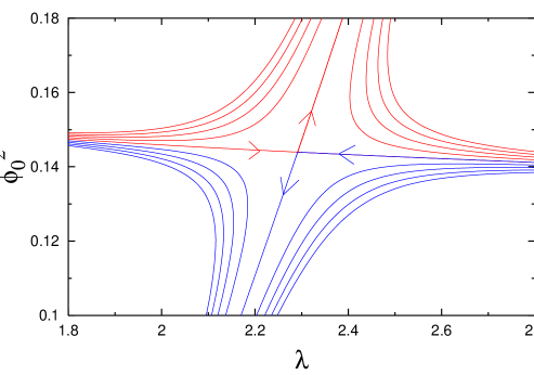
Figure 5: The mixed fixed point for $N=4$.

One nicely sees that the critical surface (line) separates both phases. When we choose initial values near the critical line the systems spends a long time near the critical point. For example starting with ${\left.\phi^{2}_{0}\right|_{t=0}}>\left.\phi^{2}_{0}\right|^{cr}_{t=0}$ and $\lambda$ finite, the evolution tends ultimately to the zero-temperature fixed point corresponding to very large values of ${\phi_{0}^{2}}$. On the other hand, starting below the critical line the evolution of ${\phi_{0}^{2}}$ tends towards the high-temperature fixed point corresponding to small values of ${\phi_{0}^{2}}$. Only for exactly ${\left.\phi^{2}_{0}\right|_{t=0}}=\left.\phi^{2}_{0}\right|^{cr}_{t=0}$ the renormalization group trajectory flows into the critical mixed fixed point, which means that the large distance behavior at the critical point is the same as that of the fixed point.

Here the predictive power of the nonperturbative approach becomes visible: During the evolution near the scaling solution the system loses memory of the initial starting value in the UV and the effective three-dimensional dynamics near the transition is completely determined by the fixed point and hence independent of the details of the considered microscopic interaction at short distances.

The equation of state drives the potential away from the critical temperature. As a result after the potential has evolved away from the scaling solution its shape is independent of the choice of the initial values such as e.g. $\lambda$ for the classical theory at the UV, signaling universal behavior near the critical point.

5.2 Beta functions

In Fig. 6 the beta function $\beta_{\lambda}\equiv\partial_{t}\lambda$ is presented as a function of $\lambda$. For $N=4$ it has two zeros at $\lambda^{*}=0$ and $\lambda^{*}=2.28$ corresponding to two fixed points. The position of the fixed points depends on the particular form of the RG flow equation encoded in the choice of the blocking function $f^{(i)}_{k}$. Physical results, however, such as critical exponents must not depend on a particular choice.

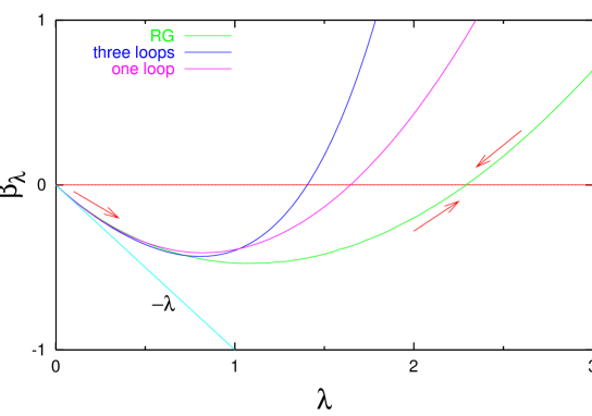
Figure 6: The beta function $\beta_{\lambda}(\lambda)$ for the $O(4)$-model. The RG result is compared to an one- and three-loop $\epsilon$-expansion for three dimensions. The arrows denote the flow w.r.t. the scale $k$ towards the infrared.

The anomalous dimension $\eta$ is nonzero at the nontrivial fixed point as shown in Fig. 7. In general it is difficult to calculate the zeros of the beta function since this requires knowledge of the physics beyond perturbation theory. The ultraviolet-stable but infrared-unstable fixed point at $\lambda^{*}=0$ is called the Gaussian fixed point because the fixed-point Hamiltonian yields a (simple) Gaussian partition function. The properties of this fixed point depend on whether the dimension $d$ is greater or less than 4. When $d$ is (slightly) smaller than 4 $\lambda$ is (slightly) relevant at the Gaussian fixed point and thus can flow to another nearby fixed point at $\lambda^{*}\approx 2.28$. This point is called the Wilson-Fisher fixed point and the flow with respect to $k$ is indicated in Fig. 6 by arrows. Thus in the limit $k\to 0$ the coupling $\lambda_{k}$ is driven to this infrared-stable fixed point because the derivative of the beta function is positive.

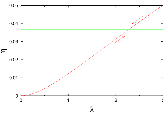
Figure 7: The anomalous dimension $\eta$ as a function of the quartic coupling $\lambda$. The flat line indicates $\eta$ at the physical vacuum.

We can also verify the large-$N$ limit: The fixed point $\lambda^{*}$ tends to zero for $N\to\infty$ merging with the Gaussian fixed point (see Table 1 and Fig. 8) [27]. When the two fixed points are sufficiently close to each other it is then possible to deduce universal properties at one fixed point in terms of those at the other one.

Figure 8: The beta function $\beta_{\lambda}(\lambda)$ for various values of $N$ demonstrating the large-$N$ behavior.

	${\phi_{0}^{2}}^{*}$	$\lambda^{*}$
N=1	0.062	3.20
N=2	0.087	2.88
N=3	0.115	2.58
N=4	0.144	2.29
N=10	0.336	1.26
N=100	3.369	0.15

Table 1: In three-dimensions the Wilson-Fisher fixed point tends towards zero in the large-$N$ limit.

Universal quantities can be calculated by perturbation theory at fixed dimension or by the $\epsilon$-expansion where the parameter $\epsilon=4-d$ is related to the number of dimension of the system. The computation of the critical exponents via the $\epsilon$-expansion beyond order ${\cal O}(\epsilon)$ requires knowledge of complicated higher-order terms in the perturbative renormalization group equations. It is believed that the $\epsilon$-expansion (including the assumption of Borel summability) is a good approximation scheme if a sufficient number of higher terms are taken into account. At the end of the calculation one has to set $\epsilon$ equal to one (or two) to obtain results of direct physical significance. One should bear in mind, however, that for a given case the $\epsilon$-expansion might be an asymptotic expansion giving eventually inaccurate results if truncated at too high an order.

In Fig. 6 we compare the beta function $\beta_{\lambda}$ for $N=4$ obtained numerically within our nonperturbative RG approach with $\epsilon$-expansions for different loop orders.

The $\epsilon$-expansion for an $O(N)$-symmetry up to three-loop order [28] is given by (for $\epsilon=1$)

$$\beta_{\lambda} = -g+\frac{(N+8)}{6}g^{2}-\frac{(3N+14)}{12}g^{3}$$

$$+\frac{33N^{2}+922N+2960+96(5N+22)\zeta(3)}{12^{3}}g^{4}+O(g^{5})$$

with $\zeta(3)=1.202057$ and the short-hand notation

$$g = \frac{12\lambda}{(4\pi)^{\frac{3}{2}}\Gamma\left(\frac{3}{2}\right)}\ .$$

At three-loop order we find agreement with our result up to $\lambda\approx 0.55$ while the one-loop order deviates from our result around $\lambda\approx 0.45$. Of course, the $\epsilon$-expansion, despite of a failure from a numerical point of view, provides an unambiguous classification of the fixed point consistent with our nonperturbative RG results.

5.3 Critical exponents and scaling relations

In the vicinity of the critical point one obtains a scaling behavior of the system which is governed by critical exponents. They parameterize the singular behavior of the free energy near the phase transition. Altogether there are six critical exponents $\alpha$, $\beta$, $\gamma$, $\delta$, $\nu$ and $\eta$ for the $O(N)$-model but only two of them are independent due to four scaling relations:

$$\alpha = 2-d\nu$$

$$\beta = \frac{\nu}{2}(d-2+\eta)$$

$$\gamma = (2-\eta)\nu$$ (32)

$$\delta = \frac{d+2-\eta}{d-2+\eta}\ .$$

In general, these universal critical exponents depend only on the dimensionality of the system $d$ and its internal symmetry. The exponents $\eta$ and $\delta$ describe the behavior of the system exactly at the critical temperature and the remaining ones parameterize the system in the region of the fixed point around $T_{c}$ ($T\neq T_{c}$).

In this work we have calculated the critical exponents $\eta$, $\beta$, $\nu$ and $\delta$ in three-dimensions numerically for different values of $N$ and could verify the scaling relations (5.3) with deviations typically being less than 0.1 $\%$. The smallness of the anomalous dimension $\eta$ (see Table 2) justifies the use of the derivative expansion of the effective action.

The critical exponent $\beta$ parameterizes the behavior of the spontaneous magnetization or the order parameter for the broken phase $(\left.{\phi_{0}^{2}}\right|_{t=0}>\left.{\phi_{0}^{2}}\right|_{t=0}^{cr})$ in the vicinity of the critical temperature (see Fig. 2). It is here numerically obtained as the slope of the logarithm of ${\phi_{0}^{2}}$ as a function of $\ln(\left.{\phi_{0}^{2}}\right|_{t=0}-\left.{\phi_{0}^{2}}\right|_{t=0}^{cr})$ for very small arguments. The difference $(\left.{\phi_{0}^{2}}\right|_{t=0}-\left.{\phi_{0}^{2}}\right|_{t=0}^{cr})$ is a measure of the distance from the phase transition irrespective of any given value $\lambda_{t=0}$ at the UV scale. If $\left.{\phi_{0}^{2}}\right|_{t=0}$ is interpreted as a function of temperature this difference is proportional to the deviation from the critical temperature i.e. proportional to $(T-T_{c})$. Thus the quantity $\left.{\phi_{0}^{2}}\right|_{t=0}^{cr}$ defines the critical temperature in three-dimensions.

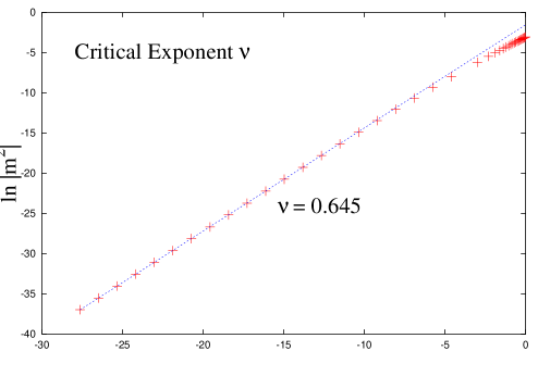
ln $\left|{\phi_{0}^{2}}|_{t=0}-{\phi_{0}^{2}}|_{t=0}^{cr}\right|$

Figure 9: The critical exponent $\nu$ for $N=4$.

The critical exponent $\nu$ describes the scaling behavior in the critical region of the renormalized mass which is the inverse of the correlation length $\xi=(T-T_{c})^{-\nu}$ and can be defined for arbitrary $N$ by the relation

$$m^{2} \sim \left|{\phi_{0}^{2}}|_{t=0}-{\phi_{0}^{2}}|_{t=0}^{cr}\right|^{2\nu}$$ (33)

with the renormalized mass in the symmetric phase $m^{2}=k^{2}u^{\prime}(0)$ for $k\to 0$. Wavefunction renormalization corrections are included in the potential. Exactly at the critical temperature i.e. for $(\left.{\phi_{0}^{2}}\right|_{t=0}=\left.{\phi_{0}^{2}}\right|_{t=0}^{cr})$ the renormalized mass vanishes and hence the correlation length diverges. For the determination of the exponent $\nu$ we calculate $m^{2}$ for different values of $\left.{\phi_{0}^{2}}\right|_{t=0}$ around $\left.{\phi_{0}^{2}}\right|_{t=0}^{cr})$ and plot $\ln(m^{2})$ as a function of $\ln\left|\left.{\phi_{0}^{2}}\right|_{t=0}-\left.{\phi_{0}^{2}}\right|_{t=0}^{cr}\right|$. The correlation is linear (see Fig. 9) and the slope yields the exponent $\nu$. Note that the definition of the renormalized mass $m^{2}$ results in a positive value only in the symmetric phase. Therefore one has to make sure to reach the symmetric phase via ${\phi_{0}^{2}}(t)\to 0$ before the evolution with respect to $t$ is stopped.

$\begin{array}[]{c}\\ \end{array}$	$\eta$	$\delta$	$\nu$	$\beta$
N=0 $\begin{array}[]{c}\mbox{RG}(1)\\ \mbox{RG}(2)\\ \mbox{lattice}\\ \epsilon\\ SPS\end{array}$	$\begin{array}[]{c}0.039\\ 0.034\\ 0.041(25)\\ 0.032(3)\\ 0.027(4)\end{array}$	$\begin{array}[]{c}4.77\\ 4.80\\ 4.77(14)\\ 4.81(2)\\ 4.84(3)\end{array}$	$\begin{array}[]{c}0.59\\ \\ 0.592(3)\\ 0.588(2)\\ 0.588(2)\end{array}$	$\begin{array}[]{c}0.30\\ \\ 0.308(6)\\ 0.304(2)\\ 0.302(2)\end{array}$
N=1 $\begin{array}[]{c}\mbox{RG}(1)\\ \mbox{RG}(2)\\ \mbox{lattice}\\ \epsilon\\ SPS\end{array}$	$\begin{array}[]{c}0.044\\ 0.045\\ 0.044(31)\\ 0.038(3)\\ 0.032(3)\end{array}$	$\begin{array}[]{c}4.75\\ 4.74\\ 4.75(17)\\ 4.78(2)\\ 4.81(2)\end{array}$	$\begin{array}[]{c}0.64\\ \\ 0.631(2)\\ 0.631(2)\\ 0.630(2)\end{array}$	$\begin{array}[]{c}0.32\\ \\ 0.329(9)\\ 0.327(2)\\ 0.325(2)\end{array}$
N=2 $\begin{array}[]{c}\mbox{RG}(1)\\ \mbox{RG}(2)\\ \mbox{lattice}\\ \epsilon\\ SPS\end{array}$	$\begin{array}[]{c}0.043\\ 0.042\\ 0.038(18)\\ 0.040(3)\\ 0.033(4)\end{array}$	$\begin{array}[]{c}4.75\\ 4.76\\ 4.78(10)\\ 4.77(2)\\ 4.81(3)\end{array}$	$\begin{array}[]{c}0.69\\ \\ 0.674(2)\\ 0.671(5)\\ 0.670(2)\end{array}$	$\begin{array}[]{c}0.35\\ \\ 0.350(5)\\ 0.349(4)\\ 0.346(2)\end{array}$
N=3 $\begin{array}[]{c}\mbox{RG}(1)\\ \mbox{RG}(2)\\ \mbox{lattice}\\ \epsilon\\ SPS\end{array}$	$\begin{array}[]{c}0.041\\ 0.038\\ 0.038(17)\\ 0.040(3)\\ 0.033(4)\end{array}$	$\begin{array}[]{c}4.76\\ 4.78\\ 4.78(10)\\ 4.77(2)\\ 4.81(3)\end{array}$	$\begin{array}[]{c}0.74\\ \\ 0.711(2)\\ 0.710(7)\\ 0.705(3)\end{array}$	$\begin{array}[]{c}0.37\\ \\ 0.369(5)\\ 0.368(4)\\ 0.365(3)\end{array}$
N=4 $\begin{array}[]{c}\mbox{RG}(1)\\ \mbox{RG}(2)\\ \mbox{lattice}\\ \epsilon\end{array}$	$\begin{array}[]{c}0.037\\ 0.034\\ 0.0254(38)\\ 0.03(1)\end{array}$	$\begin{array}[]{c}4.79\\ 4.80\\ 4.851(22)\\ 4.82(6)\end{array}$	$\begin{array}[]{c}0.78\\ \\ 0.7479(90)\\ 0.73(2)\end{array}$	$\begin{array}[]{c}0.40\\ \\ 0.3836(46)\\ 0.38(1)\end{array}$
N=7 $\begin{array}[]{c}\mbox{RG}(1)\\ \mbox{RG}(2)\end{array}$	$\begin{array}[]{c}0.027\\ 0.023\end{array}$	$\begin{array}[]{c}4.84\\ 4.87\end{array}$	$\begin{array}[]{c}0.86\\ \end{array}$	$\begin{array}[]{c}0.43\\ \end{array}$
N=10 $\begin{array}[]{c}\mbox{RG}(1)\\ \mbox{RG}(2)\end{array}$	$\begin{array}[]{c}0.021\\ 0.017\end{array}$	$\begin{array}[]{c}4.88\\ 4.90\end{array}$	$\begin{array}[]{c}0.91\\ \end{array}$	$\begin{array}[]{c}0.45\\ \end{array}$
N=100 $\begin{array}[]{c}\mbox{RG}(1)\\ \mbox{RG}(2)\end{array}$	$\begin{array}[]{c}0.0025\\ 0.002\end{array}$	$\begin{array}[]{c}4.99\\ 4.99\end{array}$	$\begin{array}[]{c}0.99\\ \end{array}$	$\begin{array}[]{c}0.49\\ \end{array}$
$\begin{array}[]{c}\\ \end{array}$large-$N$	0	5	1.0	0.5

Table 2: Critical exponents for different $N$ compared with a perturbative calculation ($SPS$), the $\epsilon$–expansion ($\epsilon$) [28] and lattice results [29]. RG(1) and RG(2) denote our results. See text for details.

In statistical physics the exponent $\delta$ describes the variation of the magnetization (here $\Phi$) in an external field $B$ in the limit $B\to 0$ at $T_{c}$:

$$B=\frac{\partial V(\Phi)}{\partial\Phi}\sim\Phi^{\delta}\ .$$ (34)

This means that the rescaled potential $u({\phi^{2}})$ is proportional to ${\phi}^{\delta+1}$ for small fields. In mean-field theory where no quantum fluctuations are taken into account the potential near the origin starts with a $\phi^{4}$-term in four-dimensions at the critical temperature. This behavior changes completely in three dimensions. In order to determine the critical exponent $\delta$ we study the flow equations in the limit ${\phi^{2}}\to\infty$ corresponding to $k\to 0$ for fixed (not rescaled) $\Phi^{2}$. In this limit $u^{\prime}$ also increases and we can therefore simplify the flow equations by neglecting the threshold functions (see Eq. (30)). At the scaling solution $\partial_{t}u=0$ (corresponding to $T=T_{c}$) we can solve the equation analytically to find

$$u_{*}({\phi^{2}})\sim{\phi}^{2d/(d-2+\eta)}\ .$$ (35)

yielding the well-known scaling relation between $\delta$ and $\eta$ (see Eq. (5.3) and [23]).

In order to extract the exponent $\delta$ numerically we calculate the first derivative of the potential $u$ w.r.t. the rescaled field ${\phi^{2}}$ and determine the slope of $\ln u^{\prime}$ for large $\ln{\phi^{2}}$.

Table 2 summarizes the resulting critical exponents $\eta$, $\delta$, $\nu$ and $\beta$ for various $N$ within our RG approach (without quoting small numerical errors). The label RG(1) denotes the numerical results for the exponents $\eta$, $\nu$ and $\beta$ which we have obtained from the scaling solution (cf. e.g. Fig. 4).

Via the scaling relations (5.3) we can, on the other hand, directly calculate $\delta$ once knowing $\eta$. The abbreviation RG(2) labels the calculated result for the exponent $\eta$. We also compare these exponents with a lattice study [29], an $\epsilon$–expansion (denoted by $\epsilon$) and to a Borel-resummed perturbative calculation up to three-loops at fixed dimension three (labeled by $SPS$) [28].

One nicely observes the convergence of all calculated critical exponents to the large-$N$ values which are quoted in the last line of Table 2. It is known that in the large-$N$ limit, the local potential approximation becomes exact and the anomalous dimension $\eta$ vanishes [9]. For the direct determination of the remaining critical exponent $\alpha$ we would have to calculate the specific heat at the critical temperature which was done in [5]. We omit the quotation of this exponent in Table 2.

5.4 The influence of the blocking functions

The structure of the regularized RG-improved flow equations (but not the universal results) depends on the $a$ $priori$ unknown cutoff function $f_{k}^{(i)}$. The index $i$ refers to the order of derivatives $(\partial^{2i})$ in the gradient expansion of the action. Thus blocking functions with $i>1$ regularize higher-order contributions to the action which go beyond the uniform wavefunction renormalization approximation, used here.

In a previous paper [4] we have studied different choices of the cutoff function for a truncated set of flow equations (A similar analysis was done in [30]). In order to see this influence for the non-truncated set of flow equations for the full potential we derive flow equations for a similar choice of the cutoff functions as in ref. [4] and calculate some critical exponents.

To be consistent with the structure of the higher momentum integrals we evaluate differential equations for each higher blocking function. Without the explicit solution of these blocking-function equations we can still find the corresponding set of flow equations (without the wavefunction contribution). We list below the corresponding flow equations for cutoff functions $i=0,1,2$ although $f_{k}^{(2)}$ is not needed in our approximation scheme:

$$f_{k}^{(0)}\ :\qquad\partial_{t}V = -\frac{k^{d}}{2}S_{d}\left[\ln(k^{2}+m^{2}_{\sigma})+(N-1)\ln(k^{2}+m^{2}_{\pi})\right]$$ (36)

$$f_{k}^{(1)}\ :\qquad\partial_{t}V = \frac{k^{d}}{d}S_{d}\left[\frac{1}{(1+m^{2}_{\sigma}/k^{2})}+\frac{N-1}{(1+m^{2}_{\pi}/k^{2})}\right]$$ (37)

$$f_{k}^{(2)}\ :\qquad\partial_{t}V = \frac{2k^{d}S_{d}}{d(d+2)}\left[\frac{1}{(1+m^{2}_{\sigma}/k^{2})^{2}}+\frac{N-1}{(1+m^{2}_{\pi}/k^{2})^{2}}\right]$$ (38)

As an example we take $N=4$ and compare the dependence of the critical exponents $\nu$ and $\beta$ on the blocking function of order $i$.

$i$	$\nu$	$\beta$
0	0.853	0.42
1	0.815	0.405
2	0.814	0.403

Table 3: The critical exponents $\nu$ and $\beta$ for $N=4$ with different blocking functions $f^{(i)}_{k}$ (without wavefunction renormalization).

In Table 3 the results are listed for various cutoff functions $f_{k}^{(i)}$. A small systematic decrease in the values with the order $i$ is observed. Already for $i\geq 1$ there is almost no difference which validates the findings in [4]. This permits the conclusion that for higher blocking functions the convergence becomes more and more stable and a decrease towards the values found by lattice simulations and $\epsilon$-expansions is observed.

6 Summary and conclusions

Near a phase-transition a perturbative treatment fails as an adequate description of the critical behavior and nonperturbative methods such as the RG method become necessary. We have presented a RG study for the finite-temperature phase transition of self-interacting scalar theories with $O(N)$-symmetry. We have used an implementation of the Wilsonian approach to field theories in thermal equilibrium which provides a direct link of the $O(N)$ universal behavior near the critical temperature with the physics at zero temperature. It offers a nonperturbative way of studying the mechanisms of dimensional reduction.

Based on an application of Schwinger’s proper-time (heat kernel) regularization within a one-loop expansion of the effective Euclidean action we have introduced various cutoff functions by comparing the proper-time regularization with a sharp-momentum regularization rendering the resulting flow equations infrared finite. This specific choice of cutoff functions has the additional advantage that all resulting flow equations can be expressed in a transparent and analytical form.

We have generalized previous studies [5],[4] to a general $O(N)$-symmetry by going beyond the local potential approximation in a derivative expansion. We have solved the highly coupled set of flow equations numerically on a grid without an specific ansatz or truncation for the potential and its derivatives during the evolution. In the infrared a convex potential is obtained for all temperatures, consistent with the concept of the effective action approach which is based on a Legendre transformation.

At the critical temperature all dimensionful quantities can be rescaled which simplifies the numerics. The dimensional reduction phenomenon which is embedded in a very transparent way in our threshold functions could be confirmed. We have discussed the critical behavior of the $O(N)$ model in detail, by determining fixed points and beta functions for various $N$. We have calculated independently four critical exponents verifying the scaling relations among them.

One important ingredient in our approach is the choice of the blocking function which is $a$ $priori$ unknown and could influence the universal quantities via the convergence properties of the flow equations. In order to control this influence we have recalculated two critical exponents ($\nu$ and $\beta$) for $N=4$ for three different choices of the blocking functions omitting the wavefunction renormalization. No strong dependence has been observed. Within numerical errors we find stable exponents except for the lowest blocking function $f_{k}^{(0)}$ due to a poor convergence. For higher blocking functions the convergence becomes more and more stable in agreement with [4].

Altogether the presented RG approach has proven to be a powerful nonperturbative tool in the study of finite-temperature field theory. Due to the omission of any temperature dependence of the initial conditions in the ultraviolet its reliability should be best for low temperature. For $N=4$ our results indeed agree perfectly with chiral perturbation theory. In contrast to chiral perturbation theory we can, however, extend the temperature range to the critical temperature where the phase transition takes place. This encourages the application of this approach to other theories involving e.g. gauge-fields.

Appendix A Appendix

In order to improve the readability of Sec. 3 we collect in this appendix some technical details concerning the derivation of the wavefunction renormalization flow equation (3).

The expansion of the effective $O(N)$-invariant Lagrangian to two-derivative order (see Eq. (7)) requires the calculation of a trace over ($N\times N$)-matrix valued terms stemming from different powers of the second derivative of the potential $V^{\prime\prime}_{ij}$ with $i,j=1,\ldots,N$.

This can basically be accomplished by introducing projectors

$$X_{1}=\frac{\Phi_{i}\Phi_{j}}{\vec{\Phi}^{2}} X_{2}=\delta_{ij}-\frac{\Phi_{i}\Phi_{j}}{\vec{\Phi}^{2}}\ ,$$ and

which satisfy the usual projection operator property $X_{a}X_{b}=\delta_{ab}X_{b}$ for $a,b=1,2$ and $trX_{1}=1$, $trX_{2}=N-1$.

Using the abbreviations $m^{2}_{\sigma}\equiv\lambda(3\vec{\Phi}^{2}-\Phi_{0}^{2})$ and $m^{2}_{\pi}\equiv\lambda(\vec{\Phi}^{2}-\Phi_{0}^{2})$ (cf. Eq. (8)) the $N\times N$ matrix $V_{ij}^{\prime\prime}$ can be rewritten by

$$V_{ij}^{\prime\prime}=\lambda\left(\vec{\Phi}^{2}-\Phi_{0}^{2}\right)\delta_{ij}+2\lambda\Phi_{i}\Phi_{j}\ =m_{\sigma}^{2}X_{1}+m_{\pi}^{2}X_{2}\ .$$

Using the projector properties different powers of $V_{ij}^{\prime\prime}$ can be readily evaluated. One finds, for example,

$$Tr\left[\sum_{n=2}^{\infty}\frac{(-1)^{n-1}\tau^{n}}{n!}\sum_{k=0}^{n-1}\left(V^{\prime\prime}\right)^{k}\partial^{2}_{\mu}\left(V^{\prime\prime}\right)^{n-1-k}\right]$$

$$\quad=-\left(\frac{1}{2}\tau^{2}\partial^{2}_{\mu}m_{\sigma}^{2}-\frac{1}{3}\tau^{3}\partial_{\mu}m_{\sigma}^{2}\partial_{\mu}m_{\sigma}^{2}\right)e^{-\tau m_{\sigma}^{2}}Tr\left[X_{1}\right]$$ (A.1)

$$\quad\quad-\left(\frac{1}{2}\tau^{2}\partial^{2}_{\mu}m_{\pi}^{2}-\frac{1}{3}\tau^{3}\partial_{\mu}m_{\pi}^{2}\partial_{\mu}m_{\pi}^{2}\right)e^{-\tau m_{\pi}^{2}}Tr\left[X_{2}\right]$$

$$\quad\quad-\left(\frac{2}{m_{\sigma}^{2}-m_{\pi}^{2}}\left(e^{-\tau m_{\pi}^{2}}-e^{-\tau m_{\sigma}^{2}}\right)-\tau\left(e^{-\tau m_{\sigma}^{2}}+e^{-\tau m_{\pi}^{2}}\right)\right)Tr\left[X_{1}\partial^{2}_{\mu}X_{1}\right]$$

where on the l.h.s. of Eq. (A) all finite and infinite sums are analytically calculable (cf. [17]) and the remaining traces are given by a straightforward calculation as

$$Tr\left[X_{a}\partial_{\mu}X_{b}\right] = 0\qquad\mbox{with}\qquad a,b,c=1,2\ ,$$

$$Tr\left[X_{a}\partial^{2}_{\mu}X_{b}\right] = 2(-1)^{\delta_{ab}+1}\left(\frac{\left(\vec{\Phi}\partial_{\mu}\vec{\Phi}\right)^{2}}{\left(\vec{\Phi}^{2}\right)^{2}}-\frac{(\partial_{\mu}\vec{\Phi})^{2}}{\vec{\Phi}^{2}}\right)\ ,$$

$$Tr\left[X_{a}\partial_{\mu}X_{b}\partial_{\mu}X_{c}\right] = (-1)^{\delta_{bc}}\left(\frac{\left(\vec{\Phi}\partial_{\mu}\vec{\Phi}\right)^{2}}{\left(\vec{\Phi}^{2}\right)^{2}}-\frac{(\partial_{\mu}\vec{\Phi})^{2}}{\vec{\Phi}^{2}}\right)\ .$$

Evaluating the other contributions to the effective action in the same manner yields Eq. (3).

References

- [1] For a review see H. Meyer-Ortmanns, Rev. Mod. Phys. 68 (1996) 473 and references therein.
- [2] L. P. Kadanoff, Physica 2 (1966) 263; K. G. Wilson, Phys. Rev. B4 (1971) 3174, 3184; K. G. Wilson and J. G. Kogut, Phys. Rev. 12 (1974) 75.
- [3] J. J. Binney, N.J. Dowrick, A.J. Fisher and M.E.J. Newman, The Theory of Critical Phenomena, Oxford University Press, 1993; M. Le Bellac, Quantum and Statistical Field Theory, Oxford University Press, 1995; J. Berges, hep-ph/9902419.
- [4] G. Papp, B.-J. Schaefer, H.-J. Pirner and J. Wambach, Phys. Rev. D61 (2000) 096002.
- [5] B.-J. Schaefer and H.-J. Pirner, Nucl. Phys. A660 (1999) 439.
- [6] C. Wetterich, Phys. Lett. B301 (1993) 90; D.-U. Jungnickel and C. Wetterich, Phys. Rev. D53 (1996) 5142; J. Berges, D.-U. Jungnickel and C. Wetterich, Phys. Rev. D59 (1999) 034010; J. Berges, N. Tetradis and C. Wetterich, hep-ph/0005122.
- [7] R. D. Ball, Phys. Rep. 182 (1989) 1; B.-J. Schaefer and H.-J. Pirner, Nucl. Phys. A627 (1997) 481.
- [8] M. D’Attanasio and M. Pietroni, Nucl. Phys. B472 (1996) 711; B. Bergerhoff and J. Reingruber, Phys. Rev. D60 (1999) 105036.
- [9] T. R. Morris, Phys. Lett. B334 (1994) 355; T. R. Morris, M. D. Turner, Nucl. Phys. B509 (1998) 637.
- [10] C. Wetterich, Z. Phys. C57 (1993) 451.
- [11] A. Bonanno, V. Branchina, H. Mohrbach and D. Zappalà, Phys. Rev. D60 (1999) 065009.
- [12] G. Ripka, Quarks Bound by Chiral Fields, Oxford University Press, 1997.
- [13] J. Schwinger, Phys. Rev. D13 (1976) 3224.
- [14] R. I. Nepomechie, Phys. Rev. D31 (1985) 3291.
- [15] C. M. Fraser, Z. Phys. C28 (1985) 101.
- [16] J. A. Zuk, Phys. Rev. D32 (1985) 2653.
- [17] M. Oleszczuk, Z. Phys. C64 (1994) 533.
- [18] S.-B. Liao, Phys. Rev. D53 (1996) 2020.
- [19] F. J. Wegner and A. Houghton, Phys. Rev. A8 (1973) 401; F. J. Wegner, in Phase Transitions and Critical Phenomena, vol. 6 eds. C. Domb and M. Greene (Academic Press, 1976).
- [20] S.-B. Liao and M. Strickland, Nucl. Phys. B532 (1998) 753.
- [21] J. Adams, J. Berges, S. Bornholdt, F. Freire, N. Tetradis and C. Wetterich, Mod. Phys. Lett. A10 (1995) 2367.
- [22] W. H. Press et al., Numerical Recipes, 2nd edition, (Cambridge University Press, 1992).
- [23] N. Tetradis and C. Wetterich, Nucl. Phys. B398 (1993) 659; M. Reuter, N. Tetradis and C. Wetterich, Nucl. Phys. B401 (1993) 567; C. Wetterich and N. Tetradis, Int. J. Mod. Phys. A9 (1994) 4029; N. Tetradis and C. Wetterich, Nucl. Phys. B422 (1994) 541.
- [24] P. Gerber and H. Leutwyler, Nucl. Phys. B321 (1989) 387.
- [25] J. Polonyi, nucl-th/9902006 Hirschegg Proceedings 1999; S.-B. Liao and J. Polonyi, Annals of Physics 222 (1993) 122.
- [26] S.-B. Liao and M. Strickland, Nucl. Phys. B497 (1997) 611.
- [27] H. J. Schnitzer, Phys. Rev. D10, 1800 (1974); S. Coleman, R. Jackiw and H.D. Politzer, Phys. Rev. D10, 2491 (1974); L.F. Abbott, J.S. Kang and H.J. Schnitzer, Phys. Rev. D13, 2212 (1976); W.A. Bardeen and M. Moshe, Phys. Rev. D28, 1372 (1983).
- [28] G. A. Baker, Jr., B. G. Nickel and D. I. Meiron, Phys. Rev. B17 (1978) 1365; G. A. Baker, Jr., B. G. Nickel , M. S. Green and D. I. Meiron, Phys. Rev. Lett. 36 (1976) 1351; J. Zinn-Justin, hep-th/0002136; J. Zinn-Justin, Quantum Field Theory and Critical Phenomena (Oxford University Press, 1990) Chapter 25 and references therein.
- [29] K. Kanaya and S. Kaya, Phys. Rev. D51 (1995) 2404.
- [30] K.I. Aoki, K. Morikawa, W. Souma, J.I Sumi and H. Terao, Prog. Theor. Phys. 99 (1998) 451; J.O Andersen, M. Strickland, cond-mat/9811096, and references therein.