Abstract

We discuss the possible signals of the degenerate BESS model at the LHC. This model describes a strongly interacting scenario responsible of the spontaneous breaking of the electroweak symmetry. It predicts two triplets of extra gauge bosons which are almost degenerate in mass. Due to this feature, the model has the property of decoupling and therefore, at low energies (below or of the order of $100\leavevmode\nobreak\ GeV$) it is nearly indistinguishable from the Standard Model. However the new resonances, both neutral and charged, should give quite spectacular signals at the LHC, where the c.o.m. energy will allow to produce these gauge bosons directly.

1 Introduction

As it is well known the Standard Model (SM) is not fully satisfactory on a theoretical basis, unless supersymmetry is present to lower the degree of divergence of the scalar sector, avoiding in this way the hierarchy problem. On the other hand, if we simply remove the Higgs from the SM, the theory becomes mathematically incomplete in the sense that it looses the remarkable property of renormalizability. Moreover, if we think to a no Higgs scenario, SM violates the unitarity limit in the scattering of longitudinal $W$ bosons around $1.7\leavevmode\nobreak\ TeV$ [1]: as a consequence it is widely believed that signals of the Higgs sector should manifest themselves below this scale and then will be apparent at the LHC where this energy scale can be probed. The BESS model [2] (BESS stands for Breaking Electroweak Symmetry Strongly) describes a physical scenario beyond the SM where the spontaneous breaking of the electroweak symmetry, necessary to give mass to the elementary particles in the SM, is driven by the dynamics of new strongly interacting fields around a mass scale of $1\leavevmode\nobreak\ TeV$. The fundamental feature of the model, in the degenerate version here considered (D-BESS) [3], consists in the decoupling property of the new sector of strong interactions at low energies ($Z$ mass). In fact, since the validity of the SM has been confirmed in the last years at the impressive level of a few per mill accuracy, only new physics which very smoothly modifies the predictions of the SM at the currently accessible energies is still conceivable. This is actually the problem of the ordinary technicolor models [4], which predict, at least in the simplest QCD rescaled version, rather big corrections to the LEP observables and then are nowadays experimentally ruled out. The easiest way to obtain small deviations from the SM predictions is to have a new sector which naturally decouples. In fact in this case, the corrections at the $Z$ energy are power suppressed in $M_{Z}/\Lambda_{np}$, where $\Lambda_{np}$ is the mass scale of the new interactions. The failure of the technicolor scenario can actually be seen as a consequence of the fact that $\Lambda_{np}\sim 250\leavevmode\nobreak\ GeV$ so that $M_{Z}/\Lambda_{np}$ is not small.
Very sketchy, we now review the model whose details can be found in [3]. If the role of the Higgs boson is taken by new strongly interacting fields, beside the Goldstone bosons, which will be absorbed by the ordinary gauge bosons, it is reasonable to assume that also vector particles will appear under the form of bound states. The model describes the low energy theory of these new vector states introducing them in the formalism of the non linear $\sigma$ model as gauge bosons of a local hidden symmetry $H=SU(2)_{L}\otimes SU(2)_{R}$ [5] [6]. This picture has been inspired by the low energy QCD where the $\rho$ resonance can be described as a gauge field [7] and in fact QCD itself can be a testing ground. In order to construct the lagrangian, we then start from the extended symmetry $G^{\prime}=G\otimes H$, where $G$ is the ordinary $SU(2)_{L}\otimes SU(2)_{R}$ of the SM which, once made local with respect to the electroweak subgroup, gives rise to the standard gauge bosons. The symmetry $G$ is spontaneously broken to the group $SU(2)_{custodial}$ to protect the relation $M_{Z}=M_{W}/\cos\theta_{W}$. This breaking produces nine Goldstone bosons which in turn disappear from the spectrum of physical particles being absorbed, through the canonical Higgs mechanism, by $W$, $Z$ and the new gauge bosons which become massive, leaving a linear combination massless. The appealing property of decoupling comes from the existence of an accidental symmetry $[SU(2)_{L}\otimes SU(2)_{R}]^{3}$ in whose correspondence the two triplets of extra-gauge bosons are degenerate in mass.
In this letter we present a simulation of the degenerate BESS model at the LHC (Large Hadron Collider) considering the Drell-Yan processes where a pair of high energy leptons is produced in the hard interaction of the protons. In particular the results have been obtained considering the CMS detector but similar results should hold also for the ATLAS experiment.
Regarding the study of the model at the existing accelerators, we refer to the second paper in ref. [3]. At LEP1 we can encode the virtual effects of the heavy resonances in the $\epsilon$ variables [8], and obtain bounds on the parameters of the model. In order to compare with the experimental data, radiative corrections have to be taken into account. Since the model is an effective description of a strongly interacting symmetry breaking sector, one has to introduce an UV cut-off $\Lambda$. We neglect the new physics loop corrections (this can be rigorously justified from the point of view of a renormalizable version of the model [9]) and assume for D-BESS the same radiative corrections as in the SM with $M_{H}=1\leavevmode\nobreak\ TeV$. As a consequence of the decoupling, the model satisfies the severe limits from LEP1 and SLC (see Figure 1) for a wide region of the parameter space without any fine tuning and even for the choice $M_{H}=1\leavevmode\nobreak\ TeV$, a value highly disfavoured by the fit within the SM.

Figure 1: 95%CL bounds on the D-BESS parameter space ($M$, $g/g^{\prime\prime}$) from LEP1/SLC (continuous line) and Tevatron upgrade at $\sqrt{s}=2\leavevmode\nobreak\ TeV$ with $L=2\leavevmode\nobreak\ fb^{-1}$(dashed line) and $L=30\leavevmode\nobreak\ fb^{-1}$ (dotted line) assuming no deviation with respect to the SM in the inclusive cross section $p\bar{p}\to\mu\nu_{\mu}$. Both the statistical error and a systematic error of 5% on the cross section have been considered. The allowed regions are under the curves.

Limits can also be obtained from the direct search of $W^{\prime}$ at the Tevatron. The present bounds are not much more restrictive than those coming from LEP1 (see [10]) but, waiting for the forthcoming upgrade, we can extrapolate them as shown in Figure 1.
The direct search of the D-BESS resonances at the Tevatron upgrade has been discussed in [10] where a simulation of the model at the LHC was presented as well. Only the muon channel of the Drell-Yan processes was considered and a very rough simulation of the energy smearing was performed. The improvement of this work consists in a much more realistic simulation of the response of the CMS detector and in the analysis of the electron channel. The CMS detector has a better energy resolution in this channel which will eventually allow to disentangle the nearly degenerate resonances, a key feature of this model, in the neutral channel for some choices of the parameters.
In section 2 we briefly recall the main features of the model underlining the differences with the ordinary strongly interacting models and giving the relevant formulas. In section 3 we report the results of the simulation at the LHC both for the neutral and charged processes in the electron and muon channels and we also discuss the possibility to disentangle the almost degenerate neutral resonances.

2 The degenerate BESS model

The D-BESS model predicts two new triplets of gauge bosons ($L^{\pm},\leavevmode\nobreak\ L_{3}$), ($R^{\pm},\leavevmode\nobreak\ R_{3}$). In comparison with the SM we have two more parameters, the common strong gauge coupling $g^{\prime\prime}$ of the triplets and the mass scale of the new sector. For this it will be convenient to choose the mass $M$ of the $R^{\pm}$ resonances.
Concerning the coupling to the fermions, we assume the same couplings as in the SM, which means that fermions are singlets of the hidden sector, even if a direct coupling is still consistent with the symmetry of the lagrangian. With this choice the new physical particles are coupled to the fermions only via the mixing with the standard particles.
The physical fields in the theory are found diagonalizing the mass matrix whose eigenvalues are the mass of the particles. In the charged sector $R^{\pm}$ are not mixed. The charged fields $W^{\pm}$ and $L^{\pm}$ have masses (the following formulas are all in the limit $M\to\infty$ and $g^{\prime\prime}\to\infty$):

$$M_{W^{\pm}}^{2} = \frac{g^{2}v^{2}}{2}$$

$$M_{L^{\pm}}^{2} = M^{2}(1+2(\frac{g}{g^{\prime\prime}})^{2})$$ (1)

$g$ the $SU(2)_{L}$ coupling of the SM and $v^{2}=1/(\sqrt{2}G_{F})$.
In the neutral sector we have:

$$M_{Z}^{2} = \frac{M_{W}^{2}}{c^{2}_{\theta}}$$

$$M^{2}_{L_{3}} = M^{2}(1+2(\frac{g}{g^{\prime\prime}})^{2})$$

$$M^{2}_{R_{3}} = M^{2}(1+2(\frac{g}{g^{\prime\prime}})^{2}\tan^{2}\theta)$$ (2)

where $\tan\theta=s_{\theta}/c_{\theta}=g^{\prime}/g$ and $g^{\prime}$ the $U(1)_{Y}$ gauge coupling and we have neglected terms which are ${\cal{O}}(1/M^{2})$. It is important to notice that the new resonances are degenerate in mass, except small corrections due to the fact that $U(1)_{Y}$ explicitly violates the custodial symmetry. The splitting between the masses in the neutral channel (the charged one is not really interesting since $R^{\pm}$ are not coupled to the fermions) at the lowest order is:

$$\Delta M=M(1-\tan^{2}\theta)\left(\frac{g}{g^{\prime\prime}}\right)^{2}$$ (3)

The couplings of the gauge bosons to the fermions can easily be obtained from the SM ones. The charged part of the fermionic lagrangian is

$${\cal L}_{charged}=-\left(a_{W}W_{\mu}^{-}+a_{L}L_{\mu}^{-}\right)J_{L}^{(+)\mu}+H.c.$$ (4)

where, in the $M\to\infty$ and $g^{\prime\prime}\to\infty$ limit,

$$a_{W} = \frac{g}{\sqrt{2}}$$

$$a_{L} = -g\frac{g}{g^{\prime\prime}}$$ (5)

and $J_{L}^{(+)\mu}={\bar{\psi}}_{L}\gamma^{\mu}\tau^{+}\psi_{L}$ with $\tau^{+}$ the combination $(\tau_{1}+i\tau_{2})/2$. Since the $R^{\pm}$ are not mixed, they are not coupled to the fermions. In the neutral sector the couplings of the fermions to the gauge bosons are (the photon is coupled in the standard way):

$$-\frac{1}{2}\bar{\psi}[(v_{Z}^{f}+a_{Z}^{f}\gamma_{5})\gamma_{\mu}Z^{\mu}+(v_{L_{3}}^{f}+a_{L_{3}}^{f}\gamma_{5})\gamma_{\mu}L_{3}^{\mu}+(v_{R_{3}}^{f}+a_{R_{3}}^{f}\gamma_{5})\gamma_{\mu}R_{3}^{\mu}]\psi$$ (6)

where $v^{f}$ and $a^{f}$ are the vector and the axial-vector couplings given by

$$v_{Z}^{f}=AT^{L}_{3}+2BQ_{em},\leavevmode\nobreak\ \leavevmode\nobreak\ \leavevmode\nobreak\ \leavevmode\nobreak\ \leavevmode\nobreak\ a_{Z}^{f}=AT^{L}_{3}$$

$$v_{L_{3}}^{f}=CT^{L}_{3}+2DQ_{em},\leavevmode\nobreak\ \leavevmode\nobreak\ \leavevmode\nobreak\ \leavevmode\nobreak\ \leavevmode\nobreak\ a_{L_{3}}^{f}=CT^{L}_{3}$$

$$v_{R_{3}}^{f}=ET^{L}_{3}+2FQ_{em},\leavevmode\nobreak\ \leavevmode\nobreak\ \leavevmode\nobreak\ \leavevmode\nobreak\ \leavevmode\nobreak\ a_{R_{3}}^{f}=ET^{L}_{3}$$ (7)

and, again in the limit $M\to\infty$, $g/g^{\prime\prime}\to 0$,

$$A =\frac{g}{c_{\theta}}\leavevmode\nobreak\ \leavevmode\nobreak\ \leavevmode\nobreak\ \leavevmode\nobreak\ B=-g\frac{s^{2}_{\theta}}{c_{\theta}}$$ (8)

$$C =-\sqrt{2}g\frac{g}{g^{\prime\prime}}\leavevmode\nobreak\ \leavevmode\nobreak\ \leavevmode\nobreak\ \leavevmode\nobreak\ D=0$$

$$E =\sqrt{2}\frac{g}{g^{\prime\prime}}\frac{g}{c_{\theta}}\tan^{2}\theta\leavevmode\nobreak\ \leavevmode\nobreak\ \leavevmode\nobreak\ \leavevmode\nobreak\ F=-E$$

The total widths in fermions are:

$$\Gamma_{L_{3}}^{fermions} = \frac{2\sqrt{2}G_{F}M_{W}^{2}}{\pi}M_{L_{3}}(g/g^{\prime\prime})^{2}$$

$$\Gamma_{R_{3}}^{fermions} = \frac{10\sqrt{2}G_{F}M_{W}^{2}}{3\pi}\frac{s_{\theta}^{4}}{c_{\theta}^{4}}M_{R_{3}}(g/g^{\prime\prime})^{2}$$

$$\Gamma_{L^{\pm}}^{fermions} = \frac{2\sqrt{2}G_{F}M_{W}^{2}}{\pi}M_{L^{\pm}}(g/g^{\prime\prime})^{2}$$ (9)

Concerning the decay in light gauge bosons we have:

$$\Gamma_{L_{3}}^{WW}=\frac{1}{48}\Gamma_{L_{3}}^{fermions}$$

$$\Gamma_{R_{3}}^{WW}=\frac{1}{80}\Gamma_{R_{3}}^{fermions}$$

$$\Gamma_{L_{3}}^{ZW}=\frac{1}{48}\Gamma_{L_{3}}^{fermions}$$ (10)

The fact that the fermionic widths are predominant is a peculiar feature of the D-BESS model. Usual models of strong breaking like technicolor predict an enhancement of the decay in longitudinal standard bosons, as it follows from the equivalence theorem [11]. The difference of the D-BESS model is related to the absence of a direct coupling between the new gauge fields and the Goldstone bosons which give mass to $W$ and $Z$. The decay in longitudinal standard bosons comes only from the mixing which is suppressed by a factor $g/g^{\prime\prime}$, then the fermionic decay is predominant due to multiplicity. For the same reason we have no additional contributions (in the leading order approximation) to the scattering of longitudinal electroweak bosons and therefore the model has the same unitarity limits as the SM.

3 Degenerate BESS at the LHC

The most suitable machine to study a new sector of strong interactions is the LHC (Large Hadron Collider), the new accelerator which will be built to shed light on the still unknown mechanism of the electroweak symmetry breaking. For a recent and detailed review of the physics at the LHC we refer to [12]. The LHC will be able either to discover the new resonances or to strongly constrain the physical region of the model.
The simulation has been performed considering the configuration of the LHC with c.o.m. energy $\sqrt{s}=14\leavevmode\nobreak\ TeV$ and an integrated luminosity of $100\leavevmode\nobreak\ fb^{-1}$, corresponding to one year of run in the so called high luminosity regime ($10^{34}\leavevmode\nobreak\ cm^{-2}s^{-1}$). However in most of the envisaged configurations the statistical significance of the signal is so high that even with an integrated luminosity of $10\leavevmode\nobreak\ fb^{-1}$, deviations from the SM will be observable.
The events were generated using Pythia Montecarlo (version 6.136) [13] and analyzed with CMSJET package [14] which performs a simulation of the CMS detector, in particular of the energy smearing. The Drell-Yan processes, where a pair of leptons emerges from the $q\bar{q}$ annihilation in a proton-proton collision, represent the golden plated signature for the D-BESS model. In fact, as we have already seen in section 2, the decay in ordinary gauge bosons is suppressed and, similarly other production processes like boson scattering are negligible. For each choice of the parameters of the model (taken inside the region still unconstrained as shown in Figure 1) we have compared the electron and the muon channels. On the theoretical point of view the processes are identical (except different radiation effects in the final states) because universality holds in the BESS model. However the electron channel is experimentally much more convenient because the CMS detector has a better energy resolution in this channel than in the muon channel (di-electron masses in the $TeV$ range can be hopefully determined with about 1% precision [15]). The energy resolution affects dramatically the shape of the resonances since we are dealing with very narrow resonances: the typical width for a $1\leavevmode\nobreak\ TeV$ boson is less than $1\leavevmode\nobreak\ GeV$ (see Tables 1 and 2).
In the charged channel we have considered the transverse mass distributions, for the inclusive process $pp\to L^{\pm},\leavevmode\nobreak\ W^{\pm}\to e\nu_{e},\leavevmode\nobreak\ \mu\nu_{\mu}$ comparing them with the SM background. Since $R^{\pm}$ are completely decoupled from the fermions they do not contribute to this process (they can be produced through the trilinear vertices of the theory but at a very low rate). Cuts have been applied in order to maximize the statistical significance of the signal, basically a cut on the low $p_{T}$ events which remove the huge SM background coming from $W$ production. We have also imposed an isolation cut on the charged leptons. The relevant background is then represented by standard Drell-Yan processes with $W$ exchange and this is the only one that we have implemented.

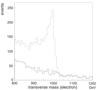
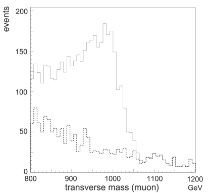
Figure 2: Transverse mass distribution of $pp\to L^{\pm},W^{\pm}\to e\nu_{e}$ events (left) and $pp\to L^{\pm},W^{\pm}\to\mu\nu_{\mu}$ (right) at the LHC with $L=100\leavevmode\nobreak\ fb^{-1}$, for $M=1000\leavevmode\nobreak\ GeV$ and $g/g^{\prime\prime}=0.1$. The dashed line represents the SM while the continuous one is D-BESS model (signal+background). The number of signal and background events and the applied cuts are given in Table 1.

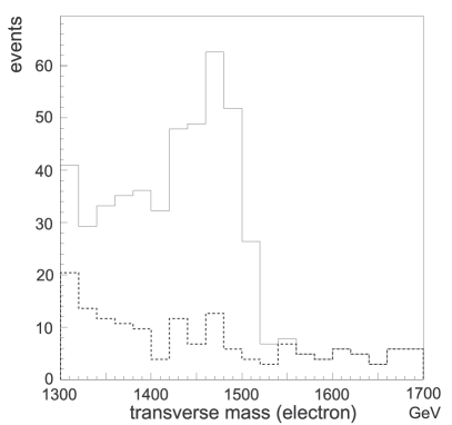
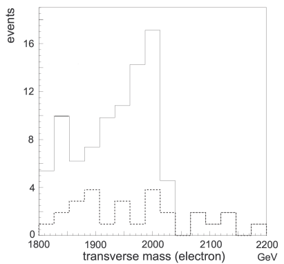
Figure 3: Transverse mass distribution of $pp\to L^{\pm},W^{\pm}\to e\nu_{e}$ events at the LHC with $L=100\leavevmode\nobreak\ fb^{-1}$, for $M=1500\leavevmode\nobreak\ GeV$ (left) and $M=2000\leavevmode\nobreak\ GeV$ (right) and $g/g^{\prime\prime}=0.1$. The number of signal and background events and the applied cuts are given in Table 1.

The distributions of the transverse mass clearly show the typical jacobian peak around the mass of the new resonances. In Figure 2 we compare the transverse mass distributions in the electron and muon channels both referring to the same choice of the D-BESS parameters and to the same applied cuts. We can notice that in the muon channel the distributions are smoother than in the electron one, due to the different energy resolution of the CMS detector.
We have analyzed the signature of the D-BESS at the LHC for several choices of the parameters (see Tables 1 and 2) chosen inside the physical region and such that they will not be ruled out by the Tevatron upgrade if no deviations from the SM are seen, as shown in Figure 1. A low mass resonance, for example $M=500\leavevmode\nobreak\ GeV$ with $g/g^{\prime\prime}=0.1$ (still within present bounds) would give a spectacular signal at the LHC, with a huge number of events and a very high statistical significance, but we don’t present this case here since it would eventually be discovered at the Tevatron. In Figure 3 we show the distributions in the electron channel corresponding to $M=1500,\leavevmode\nobreak\ 2000\leavevmode\nobreak\ GeV$ with $g/g^{\prime\prime}=0.1$: the number of events decreases for increasing mass, but the signal is quite clear because in this region the SM background is very small.
In the neutral channel we have considered the distribution of the invariant mass of a pair of leptons. We have applied cuts on the invariant mass and on the transverse momentum and we have required that both leptons were isolated in the calorimeters. These cuts kill all the non Drell-Yan backgrounds like $ZZ$, $ZW$ or $Z+jets$ or $t\bar{t}$ which in principle can give rise to decay topologies experimentally indistinguishable from di-lepton production. Although the number of events is smaller than in the charged channel, the statistical significance $S/\sqrt{S+B}$ is very high for low masses of the resonances and we derive a discovery limit at $2\leavevmode\nobreak\ TeV$ with $g/g^{\prime\prime}=0.1$. In the neutral channel we have the chance to detect the nearly degenerate resonances $L_{3},\leavevmode\nobreak\ R_{3}$ which both participate to the process: this would be the most characteristic signature of the whole model so we especially concentrate on it. In order to disentangle the double peak coming from $L_{3},\leavevmode\nobreak\ R_{3}$, a very good energy resolution is essential, so the electron channel looks the most suitable at CMS. In Figure 4 we compare the case $M=1000\leavevmode\nobreak\ GeV$ and $g/g^{\prime\prime}=0.2$ in the electron and in the muon channel. In the latest, the much wider experimental width makes it difficult to distinguish the double peak which is instead visible in the electron channel.

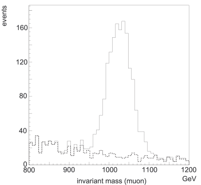
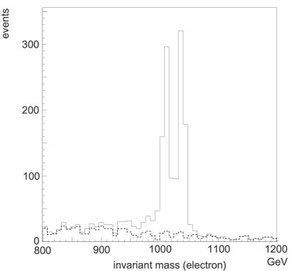
Figure 4: Invariant mass distribution of the events in $pp\to L_{3},R_{3},Z,\gamma\to\mu^{+}\mu^{-}$ (left) and in $pp\to L_{3},R_{3},Z,\gamma\to e^{+}e^{-}$ (right) at the LHC, for $M=1000\leavevmode\nobreak\ GeV$ and $g/g^{\prime\prime}=0.2$. The splitting between the resonances is $29\leavevmode\nobreak\ GeV$. The dashed line is the SM background while the continuous line represents the D-BESS model prediction (signal+background). The number of signal and background events and the applied cuts are given in Table 2.

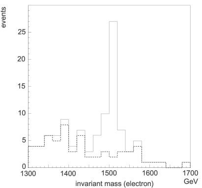
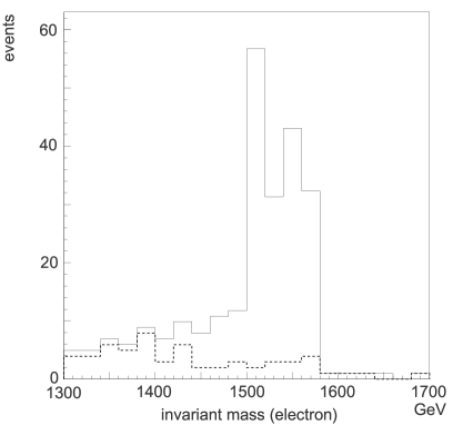
Figure 5: Invariant mass distribution of the events in $pp\to L_{3},R_{3},Z,\gamma\to e^{+}e^{-}$ at the LHC, for $M=1500\leavevmode\nobreak\ GeV$ and $g/g^{\prime\prime}=0.1\leavevmode\nobreak\ {\rm(left)};\leavevmode\nobreak\ 0.2\leavevmode\nobreak\ {\rm(right)}$. The splitting between the resonances is $10.8\leavevmode\nobreak\ GeV$ (left) and $43\leavevmode\nobreak\ GeV$ (right). The number of signal and background events and the applied cuts are given in Table 2.

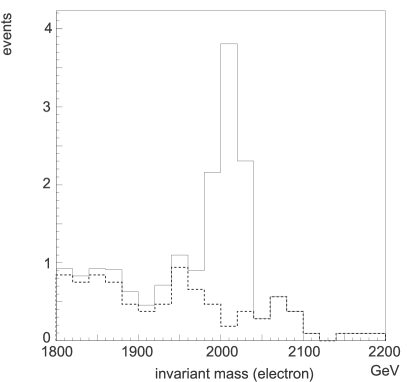
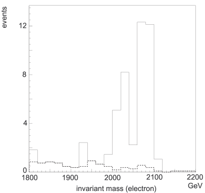
Figure 6: Same as Figure 5 for $M=2000\leavevmode\nobreak\ GeV$ and $g/g^{\prime\prime}=0.1\leavevmode\nobreak\ {\rm(left)};\leavevmode\nobreak\ 0.2\leavevmode\nobreak\ {\rm(right)}$. The splitting between the resonances is $14.3\leavevmode\nobreak\ GeV$ (left) and $57\leavevmode\nobreak\ GeV$ (right).

As in the charged channel we have considered three values of the mass of the new resonances, $1000\leavevmode\nobreak\ GeV,\leavevmode\nobreak\ 1500\leavevmode\nobreak\ GeV$ and $2000\leavevmode\nobreak\ GeV$, varying $g/g^{\prime\prime}$. The number of signal events at fixed mass shows the dependence on the parameter $g^{\prime\prime}$ of the model. In the strong coupling limit the number of events roughly scales like $1/g^{\prime\prime 2}$: this is once more a consequence of the decoupling property since, even in the limit $g^{\prime\prime}\to\infty$, we get back the SM. On the left-hand side of Figures 5 and 6, corresponding to $M=1.5,\leavevmode\nobreak\ 2\leavevmode\nobreak\ TeV$ with $g/g^{\prime\prime}=0.1$ the resonances look degenerate in the invariant mass distribution. With the choices, $M=1,1.5,2\leavevmode\nobreak\ TeV$, and $g/g^{\prime\prime}=0.2$ (right-hand side of Figures 4, 5, 6), it is instead possible to disentangle the resonances in the electron channel. The possibility to distinguish the double peak depends strongly on $g/g^{\prime\prime}$ and only smoothly on the mass. In fact, leaving aside the statistical fluctuations, this is easy to understand: what matters to disentangle the resonances is the comparison between the energy resolution and the ratio $\Delta M/M$ which is proportional to $(g/g^{\prime\prime})^{2}$ (see eq. (3)) and does not depend on $M$. In the high energy regime the energy resolution in the di-electron channel can be as lower as 1%, leading to a threshold value for $g/g^{\prime\prime}$ around 0.15. Additionally a higher value of $g/g^{\prime\prime}$ improves the statistical significance of the signal.
The results of the whole simulation are summarized in Tables 1 and 2 where we also report the cuts used in the simulation and the widths of the resonances. The number of events in the muon channel is slightly bigger than in the electron one and this is mostly due to the isolation cut on the leptons we have imposed.

$g/g^{\prime\prime}$	$M$	$\Gamma_{L^{\pm}}$	$|p_{Tl}^{c}|$	$M_{T}^{c}$	$\#B_{e}$	$\#S_{e}$	$S_{e}/\sqrt{S_{e}+B_{e}}$	$\#B_{\mu}$	$\#S_{\mu}$
	(GeV)	(GeV)	(GeV)	(GeV)
0.1	1000	0.7	300	800	1468	2679	41.6	1529	2876
0.1	1500	1.0	500	1300	154	339	15.3	166	422
0.1	2000	1.4	700	1800	26	67	6.9	31	92

Table 1: D-BESS model at the LHC for the process $pp\to e\nu_{e}(\mu\nu_{\mu})+X$. #B(#S) corresponds to the number of background (signal) events. Also shown are the width of $L^{\pm}$ and the applied cuts on the $p_{T}$ of the lepton and on the transverse mass.

$g/g^{\prime\prime}$	$M$	$\Gamma_{L_{3}}$	$\Gamma_{R_{3}}$	$|p_{Tl}^{c}|$	$m^{c}_{e^{+}e^{-}(\mu^{+}\mu^{-})}$	$\#B_{e}$	$\#S_{e}$	$S_{e}/\sqrt{S_{e}+B_{e}}$	$\#B_{\mu}$	$\#S_{\mu}$
	(GeV)	(GeV)	(GeV)	(GeV)	(GeV)
0.1	1000	0.7	0.1	300	800	590	375	12	680	411
0.2	1000	2.8	0.4	300	800	590	1342	31	680	1520
0.1	1500	1.0	0.15	500	1300	58	46	4.5	71	69
0.2	1500	4.0	0.6	500	1300	58	189	12	71	247
0.1	2000	1.4	0.2	700	1800	9	9	2.1	12	16
0.2	2000	5.6	0.8	700	1800	9	43	6.0	12	52

Table 2: D-BESS model at the LHC for the process $pp\to e^{+}e^{-}(\mu^{+}\mu^{-})+X$. #B(#S) corresponds to the number of background (signal) events. Also shown are the widths of $L_{3}$ and $R_{3}$ and the applied cuts on the $p_{T}$ of the leptons and on the invariant mass.

4 Conclusions

We have shown the possible signals at the LHC of a dynamical symmetry breaking model called degenerate BESS, which predicts two triplets of new vector resonances, almost degenerate in mass. The model has the appealing property of decoupling which makes it automatically pass all the low energy tests, leaving the possibility of a strong sector of interactions even at rather low energies.
The neutral channel represents the clearest signature of the model if it is possible to disentangle the two resonances. However, the production rate is less favorable than in the charged one, exactly as it happens in the SM, since we have considered a minimal coupling to fermions. The neutral gauge bosons can be detected over the background up to $M=2000\leavevmode\nobreak\ GeV$, provided $g/g^{\prime\prime}$ is not smaller than $0.1$. In the charged channel, where only the $L^{\pm}$ bosons contribute to the signal, the limit of detection at $2\leavevmode\nobreak\ TeV$ is reached for $g/g^{\prime\prime}=0.03$, but the experimental proof of the model requires that both neutral and charged resonances are discovered. We have compared the electron and muon channels coming to the conclusion that the first is experimentally more convenient since the CMS detector has a better energy resolution for the electrons than the muons in the high energy range.
If the new particles will not be discovered at the LHC, very restrictive limits on the parameter space could be derived, which, in the light of the unitarity limit of the model, will essentially close the physical region of the D-BESS model.

Figure 7: 95%CL limits on the parameter space ($M$, $g/g^{\prime\prime}$) of the D-BESS model at the LHC with $L=100\leavevmode\nobreak\ fb^{-1}$ (dotted-dashed line) and $L=10\leavevmode\nobreak\ fb^{-1}$ (dotted line) assuming no deviations are seen from the SM in the cross section $pp\to\mu\nu_{\mu}$. Both the statistical error and a systematic error of 5% have been taken into account. The continuous line corresponds to the present LEP1/SLC bound.

In fact, if no deviations from the SM are seen at the LHC, the bounds shown in Figure 7 can be drawn.

Acknowledgement:
We thank S. Abdulline for allowing us to use the CMSJET package and for his helpful advice.

References

- [1] B.W. Lee, C. Quigg and H.B. Thacker, Phys. Rev. D16 (1977) 1519; Phys. Rev. Lett. 16 (1977) 883.
- [2] R. Casalbuoni, S. De Curtis, D. Dominici and R.Gatto, Phys. Lett. B155 (1985) 95; Nucl. Phys. B282 (1987) 235.
- [3] R. Casalbuoni, A. Deandrea, S. De Curtis, D. Dominici, F. Feruglio, R. Gatto and M. Grazzini, Phys. Lett. B349 (1995) 533; R. Casalbuoni, A. Deandrea, S. De Curtis, D. Dominici, R. Gatto and M. Grazzini, Phys. Rev. D53 (1996) 5201.
- [4] S. Weinberg, Phys. Rev. D19,(1979) 1277; L. Susskind, Phys. Rev. D20, (1979) 2619.
- [5] C.G. Callan, S. Coleman, J. Wess and B. Zumino, Phys. Rev. 177 (1969) 2239; S. Coleman, J. Wess and B. Zumino, Phys. Rev. 177 (1969) 2247.
- [6] A.P. Balachandran, A. Stern and G. Trahern, Phys Rev. D19 (1979) 2416; M. Bando, T. Kugo, S. Uehara and K. Ynagida, Phys. Rev. Lett. 54 (1985) 1215; M. Bando, T. Kugo and K. Yamawaki, Prog. Theor. Phys. 73 (1985) 1541.
- [7] M. Bando, T. Kugo and K. Yamawaki, Phys. Rep. 164 (1988) 217.
- [8] G. Altarelli and R. Barbieri, Phys. Lett. B253 (1991) 161; G. Altarelli, R. Barbieri and S. Jadach, Nucl. Phys. B369 (1992) 3; G. Altarelli, R. Barbieri and F. Caravaglios, Nucl. Phys. B405 (1993) 3.
- [9] R. Casalbuoni, S. De Curtis, D. Dominici, M. Grazzini, Phys. Rev. D56 (1997) 5731.
- [10] R. Casalbuoni, P. Chiappetta, A. Deandrea, S. De Curtis, D. Dominici and R. Gatto, Phys. Rev. D56, (1997) 2812.
- [11] J.M. Cornwall, D.N. Levin and G. Tiktopoulous, Phys. Rev. D10 (1974) 1145; C.G. Vayonakis, Lett. Nuovo Cimento 17 1976 17; M.S. Chanowitz and M.K. Gaillard, Nucl. Phys. B261 (1985) 379; G.J. Gounaris, R. Kogerler and H. Neufeld, Phys. Rev. D34 (1986) 3257; Y. Yao, C.P. Yuan, Phys. Rev. D38 (1988) 2237; J. Bagger and C.R. Schmidt, Phys. Rev. D41 (1990) 264; H. Veltman, Phys. Rev. D41 (1990) 2294; H.J. He, Y.P. Kuang and X. Li, Phys. Rev. Lett. 69 (1992) 2619; Phys. Lett. B329 (1994) 278.
- [12] S. Haywood et al., ”Electroweak physics”, CERN-YR-2000/01, edited by G. Altarelli and M.L. Mangano.
- [13] T. Sjostrand, Comp. Phys. Comm. 82 (1994) 74.
-
[14]
S. Abdullin, A. Khanov, N. Stefanov, CMS TN/94-180
http://cmsdoc.cern.ch/abdullin/cmsjet.html - [15] D. Denegri, private communication.