Abstract

We use the recent estimates of NNLO splitting functions, made by van Neerven and Vogt, to perform exploratory fits to deep inelastic and related hard scattering data. We investigate the hierarchy of parton distributions obtained at LO, NLO and NNLO, and, more important, the stability of the resulting predictions for physical observables. We use the longitudinal structure function $F_{L}$ and the cross sections $\sigma_{W},\sigma_{Z}$ for $W$ and $Z$ hadroproduction as examples. For $F_{L}$ we find relatively poor convergence, with increasing order, at small $x$; whereas $\sigma_{W,Z}$ are much more reliably predicted.

1 Introduction

With the increased precision of deep inelastic scattering data [1], and the need for accurate predictions at the Tevatron and the LHC, it is clearly essential to extend global parton analyses to next-to-next-leading-order (NNLO) in $\alpha_{S}$. Although the relevant deep inelastic coefficient functions have been known for some time [2], there is only partial information on the corresponding splitting functions. The $N=2,4,6,8$ (and 10 for non-singlet) moments have been calculated [3], which effectively provide information on the high $x$ behaviour of the splitting functions. Also known is the most singular $\log 1/x$ behaviour at small $x$, both for the singlet [4], and the phenomenologically less important nonsinglet [5] splitting functions, and the leading $n_{f}$ contributions [6] of the nonsinglet splitting functions, and of the $C_{A}$ dependent part of $P_{gg}$ [7]. Recently van Neerven and Vogt [8] have constructed compact analytic expressions for the splitting functions which represent the fastest and the slowest evolution that is consistent with the above information. We believe that these two extreme behaviours are indeed realistic. Although there are indications that the true behaviour of the splitting functions is likely to be slightly nearer to that corresponding to the slow evolution possibility, for simplicity we shall use the average of the two extremes for our ‘central’ NNLO analysis.

It is important to stress an important difference between our analysis and the procedure used by van Neerven and Vogt [8]. The latter authors start from a fixed set of partons and a fixed scale ($\sim 30$ GeV² i.e $\alpha_{S}=0.2$) and present the differences between LO, NLO and NNLO evolution. Here we compare the partons, and the consequent predictions for physical observables, obtained by performing global analyses at LO, NLO and NNLO. Both works present NNLO results obtained using the extreme estimates of the ${\cal O}(\alpha_{S}^{3})$ splitting functions.

In Section 2 we discuss the changes to the global analysis that are necessary in going from a NLO to NNLO formulation. Then, in Section 3, we present seven new fits to the deep inelastic and related data; that is LO, NLO and five NNLO analyses. To gain insight into the impact of the NNLO contributions, we discuss essential features of the fits in terms of the behaviour of the splitting (and coefficient) functions. In Section 4 we compare the partons obtained in the LO, NLO and NNLO analyses, paying particular attention to the gluon distribution in the small $x$ region. The parton distributions are scheme dependent and are not themselves observable. The comparison of LO, NLO and NNLO predictions for physical observables is much more meaningful. In Section 5 we study the predictions for the longitudinal structure function, $F_{L}$. This is a particularly relevant observable as it directly reflects the behaviour of the gluon distribution at small $x$, and hence most directly probes the stability, or convergence, of parton analyses as we go from the LO, to the NLO, and then to the NNLO framework. In Section 6 we compare the LO, NLO, NNLO predictions for the cross sections of $W$ and $Z$ boson production at the Tevatron $p\bar{p}$ collider and at the LHC. These observables mainly depend on the quark distributions in the region $Q^{2}\sim 10^{4}$ GeV², and $x\sim 0.05$ and 0.006 respectively. The stability of the predictions offers the possibility of using the $W$ and $Z$ events as a luminosity monitor of the collider. Finally in Section 7 we give our conclusions.

2 Global analyses at NNLO

The procedure is based on the NLO analyses described in Refs. [9, 10]. However at NNLO it is important to allow the gluon distribution to become negative in the low $x$, low $Q^{2}$ domain. We therefore adopt the parameterization

$$xg(x,Q_{0}^{2})\;=\;A_{g}\>x^{-\lambda_{g}}\>(1-x)^{\eta_{g}}\>(1+\varepsilon_{g}\sqrt{x}+\gamma_{g}x)\>-\>A_{g}^{\prime}\>x^{-\lambda_{g}^{\prime}}\>(1-x)^{\eta_{g}^{\prime}}$$ (1)

at the starting scale $Q^{2}=Q_{0}^{2}=1~{}{\rm GeV}^{2}$ of the evolution. The parameter $\eta_{g}^{\prime}$ turns out to be large in the additional negative term and so this contribution is only important at small $x$.

It is necessary to implement other extensions of the formalism when going to NNLO. First, we use the three-loop expression for $\alpha_{S}$, in the $\overline{\rm MS}$ scheme. Second, we require more detailed matching conditions when evolving through the heavy flavour thresholds. The NNLO treatment of heavy flavours is discussed in the Appendix.

Our main interest is in the quality of the fit to deep inelastic data at small $x$. At high $x$ we have a slight inconsistency in our NNLO analyses in that we use NLO expressions to fit to Drell-Yan, jet production and $W^{\pm}$ boson rapidity asymmetry. The NNLO corrections to all these quantities have not yet been calculated. However note that the physical observables that we study (namely $F_{L}$ and $\sigma_{W,Z}$) sample low $x$ partons, which are determined mainly by deep inelastic data for which the NNLO formalism is consistent.

3 The new global fits

We perform LO, NLO and NNLO global fits to the set of deep inelastic and related data that was used in Refs. [9, 10], except that now we use the jet $E_{T}$ distribution measured at the Tevatron to pin down the gluon distribution at large $x$, instead of prompt photon hadroproduction. The QCD description of the latter process has outstanding theoretical problems [11]. A second change is that we include all the available preliminary HERA data [1], which have higher precision than hitherto.

The consequence of replacing prompt photon data by the jet data is that the NLO fit is now similar to that achieved by the previous MRST($g\!\!\uparrow$) set of partons [9, 10]. A satisfactory description of the Tevatron jet data is obtained, including particularly the normalization.

Five NNLO fits were performed. The ‘central’ fit and the four extremes ($A_{q}A_{g},A_{q}B_{g},B_{q}A_{g},\linebreak B_{q}B_{g}$), where $A_{i}(B_{i})$ corresponds to the slow (fast) evolution of parton $i=q,g$. It turns out that the NNLO fits with slow and fast gluon evolution are very similar, and so it is sufficient to present results for just two of the extreme choices of the splitting functions, namely

$$A \equiv A_{q}A_{g}~{}~{}~{}({\rm slow~{}evolution}),$$

$$B \equiv B_{q}B_{g}~{}~{}~{}({\rm fast~{}evolution}).$$ (2)

In Figs. 1 and 2 we show the LO, NLO and NNLO descriptions of the $F_{2}$ data [12] in a few representative $x$ bins. We display only the ‘central’ NNLO fit. However the quality of all the NNLO fits is similar. It is encouraging to note that, as we proceed from the LO $\rightarrow$ NLO $\rightarrow$ NNLO analysis, there is sequential improvement in the overall quality of the description of the data. In particular, in going from the NLO $\rightarrow$ NNLO fit, there is an improvement in the simultaneous description of the NMC and HERA $F_{2}$ data. Indeed the quality of the NNLO fit is improved for almost all subsets of the data.

From Figs. 1 and 2 we can see that at NNLO the scaling violations increase both at small $x$ and at large $x$. At small $x$ this is due mainly to the NNLO contribution to $P_{qg}$, whereas at large $x$ the NNLO term in the coefficient function plays the dominant role. The relevant $x\rightarrow 0$ behaviour of the splitting functions are

$$P_{qg}(x) = 2n_{f}\frac{\alpha_{S}}{2\pi}\frac{1}{3}\biggl{(}1+\frac{5}{3}\frac{\bar{\alpha}_{S}}{x}+\frac{14}{9}\frac{\bar{\alpha}_{S}^{2}\ln(1/x)}{x}+\cdots\biggr{)}$$ (3)

$$P_{gg}(x) = \frac{\bar{\alpha}_{S}}{x}\left[1-\frac{61n_{f}}{36}\frac{\bar{\alpha}_{S}}{x}-\biggl{(}\frac{395}{104}-\frac{1}{2}\zeta(3)-\frac{11\pi^{2}}{72}+n_{f}\biggl{(}\frac{295}{2808}-\frac{\pi^{2}}{972}\biggr{)}\biggr{)}\frac{\bar{\alpha}_{S}^{2}\ln(1/x)}{x}\right],$$ (4)

where $\bar{\alpha}_{S}=(3/\pi)\alpha_{S}$, and the $x\rightarrow 1$ behaviour of the quark contribution to the $F_{2}$ coefficient function is

$$C_{2,q}(x)\;=\;\delta(1-x)+\frac{\alpha_{S}}{4\pi}C_{F}\biggl{(}\frac{4\ln(1-x)-3}{1-x}\biggr{)}_{+}$$

$$\quad+\;\left(\frac{\alpha_{S}}{4\pi}\right)^{2}\left[8C_{F}^{2}\left(\frac{\ln^{3}(1-x)}{1-x}\right)_{+}+\left(-\frac{22}{3}C_{A}C_{F}+\frac{4}{3}C_{F}n_{f}-18C_{F}^{2}\right)\left(\frac{\ln^{2}(1-x)}{1-x}\right)_{+}\right].$$ (5)

As well as the improvement in the quality of the fit, we can investigate the importance of the increased scaling violations by looking at the higher-twist component of $F_{2}$ extracted using a phenomenological analysis in which a term $(D(x)/Q^{2})F_{2}(x,Q^{2})$ is included in the fit, as in Ref. [13]. The values of the higher-twist coefficient $D(x)$ can be seen in Table 1. At very high $x$ a large positive higher-twist contribution is clearly needed. This decreases slightly as we move from LO to NLO to NNLO, but there is no indication that its presence will be eliminated by even higher orders. We note that the conclusion that NNLO contributions largely remove the need for higher twist at high $x$ in previous NNLO analyses [14] has been based on analysis of CCFR data only, which exists at far higher $W^{2}$ than the SLAC data included in our higher-twist fit, though it has also been suggested that when NNLO coefficient functions are used the higher twist may be almost entirely due to target mass effects [15]. At $x=0.4\to 0.5$ the higher-twist contribution changes sign, becoming generally negative. At LO its magnitude is then quite large, demonstrating that the evolution is too slow at low $Q^{2}$, both for NMC and HERA data, as is obvious from Fig. 1. The magnitude of the higher-twist contribution for $x<0.3$ decreases significantly going to NLO, and decreases again, to very small values, at NNLO. Indeed, the sign of the small-$x$ higher-twist contributions at NNLO is not even well-determined, with many $x$-bins preferring a slightly positive value. The implication seems to be that higher-twist contributions at small $x$ are small, and their apparent size is decreased by the inclusion of more perturbative corrections.

Table 1: Values of the higher-twist coefficient $D(x)$ extracted from the LO, NLO and NNLO fits

$x$	LO	NLO	NNLO
0 – 0.0005	$-$0.4754	0.0116	$-$0.0061
0.0005 – 0.005	$-$0.2512	$-$0.0475	0.0437
0.005 – 0.01	$-$0.2481	$-$0.1376	$-$0.0048
0.01 – 0.06	$-$0.2306	$-$0.1271	$-$0.0359
0.06 – 0.1	$-$0.1373	$-$0.0321	0.0167
0.1 – 0.2	$-$0.1263	$-$0.0361	0.0075
0.2 – 0.3	$-$0.1210	$-$0.0893	$-$0.0201
0.3 – 0.4	$-$0.0909	$-$0.1710	$-$0.1170
0.4 – 0.5	0.1788	$-$0.0804	$-$0.0782
0.5 – 0.6	0.8329	0.3056	0.1936
0.6 – 0.7	2.544	1.621	1.263
0.7 – 0.8	6.914	5.468	4.557
0.8 – 0.9	19.92	18.03	15.38

For each fit – LO, NLO, NNLO – we use the one-, two-, three-loop expression for the $\beta$ function, e.g. in the NNLO fits the connection between $\alpha_{S}$ and $\Lambda_{\overline{\rm MS}}$ involves $\beta_{2}$ evaluated in the $\overline{\rm MS}$ scheme. For completeness we show in Table 2 the values of the QCD coupling, together with $\Lambda_{\rm QCD}$, found in the different global fits. For the NNLO fits the value of $\Lambda_{\rm QCD}$ is kept the same for the extremes as for the central fit, but would change by only a tiny amount if left free. In the fits where a higher-twist component is allowed, at each order the extracted value of $\Lambda_{\rm QCD}$ increases, reflecting the effect of the increased scaling violation by the new data at low $Q^{2}$ included in these fits. This increase in $\Lambda_{\rm QCD}$ is only $10-15\%$ (decreasing with increasing order), leading to a corresponding increase in $\alpha_{S}(M_{Z}^{2})$ of $0.002-0.003$.

Table 2: The QCD coupling and $\Lambda$ parameter

	$\alpha_{S}(M_{Z}^{2})$	$\Lambda_{\rm{LO\;\;or\;\;}\overline{\rm MS}}^{(n_{f}=4)}~{}({\rm GeV})$
LO	0.1253	0.174
NLO	0.1175	0.300
(NNLO)central	0.1161	0.242
(NNLO)A	0.1161	0.242
(NNLO)B	0.1161	0.242

4 Implications for parton distributions

In Fig. 3 we compare the parton distributions found in the NNLO fit to those in the NLO analysis. We plot the NNLO/NLO ratios for the gluon, and the up and down quark distributions, at two values of $Q^{2}$.

As we go from the NLO to the NNLO analysis, several changes in the distributions are worth noting. First, the decrease of the quark distribution at high $x$ and the slight increase at low $x$ reflect the behaviour of the coefficient functions $C_{2,q}$ and $C_{2,g}$ respectively. Second, recall that in the NLO analysis the input gluon distribution decreased at small $x$. At NNLO we see the gluon decreases even more. This decrease at low $x$ occurs because of the increase of $P_{qg}$, see (3). The consequent rise at $x\sim 0.1$ is to ensure that the momentum sum rule is satisfied. The gluon distribution drives the evolution at small $x$. As we evolve to higher $Q^{2}$, the effect of the NNLO term in the splitting function decreases, and a smaller gluon leads to slower evolution than in the NLO analysis. Hence, for example, by $Q^{2}\sim 10^{4}$ GeV and $x\sim 10^{-4}$, all NNLO partons are about 10–15% smaller than those at NLO.

Since the biggest NNLO effect is in the small $x$ behaviour of the gluon, we study this distribution in more detail. Fig. 4 shows the gluon obtained in the LO, NLO and NNLO global fits at various values of $Q^{2}$. A clear LO $\rightarrow$ NLO $\rightarrow$ NNLO hierarchy of the small $x$ behaviour of the gluon is evident, which reflects the direct link with the HERA deep inelastic data via $P_{qg}$ of (3). Note also that the evolution of the NNLO gluon is made even slower because of the (small) negative NNLO contribution in $P_{gg}$, see (4).

The ‘starting’ parametric forms of the gluon found in the LO, NLO and NNLO global analyses are

$$xg(x,Q_{0}^{2})\;=$$

$$=\;\left\{\begin{array}[]{l}31.2x^{0.390}(1-x)^{6.18}\>(1-5.23\sqrt{x}+7.33x)\quad\quad\quad\quad\quad\quad\quad\quad\quad\quad\quad\quad\quad\>({\rm LO})\\ 51.8x^{0.535}(1-x)^{6.55}\>(1-3.92\sqrt{x}+4.68x)-1.67x^{-0.032}(1-x)^{8.21}\quad\quad\>({\rm NLO})\\ 14.4x^{0.397}(1-x)^{5.56}\>(1-3.22\sqrt{x}+4.36x)-0.705x^{-0.151}(1-x)^{8.69}.~{}~{}({\rm NNLO})\end{array}\right.$$ (9)

The ‘extreme’ curves $A$ and $B$, plotted in Fig. 4, demonstrate that the greatest uncertainty, coming from the lack of complete knowledge of the NNLO splitting functions, is in the small $x$ behaviour of the gluon. Nevertheless even allowing for the ‘extreme’ spread in the NNLO fits we see that the hierarchy in the small $x$ behaviour of the gluon persists.

Fig. 4 also shows that the gluon obtained from the NNLO analysis becomes negative at small $x$ and small $Q^{2}$, as anticipated in (1). However the gluon distribution itself is not a physically observable quantity. It is scheme dependent. For example, Fig. 4 shows the gluons obtained from analyses at different orders in the $\overline{\rm MS}$ factorization scheme. If on the other hand we were to adopt the DIS scheme, then we find that the NNLO gluon is only marginally negative at low $x$ at $Q^{2}=2$ GeV². In order to investigate the true implications of the convergence of the perturbative series we must examine the predictions for physically observable quantities. The behaviour of the longitudinal structure function, $F_{L}$, is particularly appropriate as it is sensitive to the small $x$ behaviour of the gluon. The production cross sections of $W$ and $Z$ bosons at the hadron colliders are representative of other relevant observables. We therefore study the predictions for these quantities below.

5 Predictions for $F_{L}$

The LO contribution to $F_{L}$ is ${\cal O}(\alpha_{S})$, and so a consistent (factorization scheme independent) NNLO prediction of $F_{L}$ requires the ${\cal O}(\alpha_{S}^{3})$ coefficient functions. These are not known at present, but we do know much of the same information as for the ${\cal O}(\alpha_{S}^{3})$ splitting functions, that is the $N=2,4,6,8$ moments and the $x\to 0$ behaviour. Hence we estimate the coefficient functions in the same spirit as used by van Neerven and Vogt for the ${\cal O}(\alpha_{S}^{3})$ splitting functions. The ‘central’ estimates for the NNLO contributions to $C_{L}$ are (where the common factor of $(\alpha_{S}/(4\pi))^{3}$ is taken out)

$$C_{L,g}^{(3)}(x) = \Biggl{[}n_{f}\biggl{(}381\frac{\ln(1/x)}{x}-\frac{1200}{x}+1095\ln^{2}(1/x)-5960+21512x^{2}+1928\ln(1-x)\biggl{)}$$ (10)

$$+n_{f}^{2}\biggl{(}\frac{20}{x}+148.8\ln^{2}(1/x)-5-741x^{2}-147\ln(1-x)\biggr{)}\Biggr{]}$$

$$C_{L,{\rm NS}}^{(3)}(x) = \Biggl{[}\biggl{(}-323\ln^{2}(1/x)-3916-47526x^{2}-21954\ln(1-x)\biggr{)}$$ (11)

$$+n_{f}\biggl{(}-89\ln^{2}(1/x)+863+2796x^{2}+2038\ln(1-x)\biggr{)}$$

$$+n_{f}^{2}\biggl{(}15\ln^{2}(1/x)-54.3+72.4x^{2}-23\ln(1-x)\biggl{)}\Biggr{]}$$

$$C_{L,{\rm PS}}^{(3)}(x) = \Biggl{[}n_{f}\biggl{(}\frac{169\ln(1/x)}{x}-\frac{700}{x}+186\ln^{2}(1/x)+578x^{2}+42.6\ln(1-x)+316\biggr{)}$$ (12)

$$+n_{f}^{2}\biggl{(}\frac{10}{x}+61\ln^{2}(1/x)-25+42.7x^{2}+7.2\ln(1-x)\biggr{)}\Biggr{]}$$

where NS and PS refer to quark non-singlet and pure-singlet respectively. In fact the $n_{f}^{2}$ dependent part of the non-singlet coefficient function is in principle known exactly from the calculations in [16], but are small and well modelled by our simple analytic expression.

The behaviour of the $F_{L}$ gluon coefficient function is shown in Fig. 5. The two dominant features are (i) a sizeable contribution just below $x=1$, and (ii) a large growth with decreasing $x$ arising from the most singular terms found in Ref. [4]. In fact at small $x$ we have

$$C_{L,g}(x)\;\simeq\;\frac{\alpha_{S}}{2\pi}n_{f}\frac{2}{3}\left[1-\frac{1}{3}\frac{\bar{\alpha}_{S}}{x}+\left(\frac{43}{9}-\zeta(2)\right)\frac{\bar{\alpha}_{S}^{2}\ln(1/x)}{x}\right]$$ (13)

and the same expression, modulo the colour factor $C_{F}/C_{A}=4/9$, for $C_{L,{\rm PS}}$ (except at leading order).

The non-singlet coefficient functions beyond LO are very strongly peaked as $x\to 1$. At NLO the coefficient function [17] (with $(\alpha_{S}/(4\pi))^{2}$ factored out) in this limit behaves like

$$C^{(2)}_{L,{\rm NS}}(x) \simeq 4C_{F}\biggl{[}2C_{F}\ln^{2}(1-x)+(9-8\zeta(2))C_{F}\ln(1-x)$$ (14)

$$+\biggl{(}4(\zeta(2)-1)C_{A}-\bigl{(}11-\frac{2}{3}n_{f}\bigr{)}\biggr{)}\ln(1-x)\Biggr{]},$$

and there is an enhancement compared to the LO result, $(\alpha_{S}/(4\pi))4C_{F}x$, due to the $\ln(1-x)$ terms. The machinery for computing the dominant $\ln(1-x)$ terms for $C_{L,{\rm NS}}$ for all orders in $\alpha_{S}$ has recently been devised [18], and in principle we could use this to evaluate the parts $\propto\ln^{m}(1-x)$ at ${\cal O}(\alpha_{S}^{3})$ for $m=2,3,4$. However, the resulting expressions are very far from compact and at this order we simply choose to use the the information on the moments which is available to give us a good estimate of the coefficient function at high $x$. This confirms that again the coefficient function is very peaked for $x\to 1$ – its size largely compensating for the extra power of $\alpha_{S}/(4\pi)$. A more sophisticated parameterization than that used in (12) should really include higher powers in $\ln(1-x)$, but since the expression matches a range of moments very well it will give an accurate representation of the coefficient function convoluted with the smooth parton density.

The predictions for $F_{L}$ obtained from the parton distributions of the different global fits are shown in Fig. 6. The progressive increase at high $x$ is attributable to the large NS coefficient functions for $x\to 1$. At small $x$ the LO and NLO predictions mirror the gluon distribution (sampled in the region of $2x$ due to the convolution). The NNLO prediction of $F_{L}$ also mirrors the shape of the gluon at low $Q^{2}$ and moderate $x$, turning over at $x\sim 0.05$. Then, at even smaller $x$, the very large ${\cal O}(\alpha_{S}^{3})$ contribution of $C_{L,g}$ takes over, which after convolution with the gluon, prevents $F_{L}$ becoming negative and, in fact, results in a steep rise with decreasing $x$. As we evolve up in $Q^{2}$ the effect of the ${\cal O}(\alpha_{S}^{3})$ term in $C_{L,g}$ diminishes and eventually the NNLO prediction for $F_{L}$ mirrors the shape and size of the gluon via the ${\cal O}(\alpha_{S})$ term in $C_{L,g}$. Hence there is a transition at $Q^{2}\sim 5~{}{\rm GeV}^{2}$ where the NLO overtakes the NNLO prediction of $F_{L}$. At the lowest values of $Q^{2}$ the NNLO prediction of $F_{L}$ should be regarded with caution. If we go below $Q^{2}=2$ GeV² the dip in $F_{L}$ in Fig. 6 becomes negative, indicating the unreliability of the NNLO analysis in this domain.

In the region $Q\lower 3.01385pt\hbox{$\;\stackrel{{\scriptstyle\textstyle>}}{{\sim}}\;$}20$ GeV², Fig. 6 shows a LO $\rightarrow$ NLO $\rightarrow$ NNLO hierarchy in the small $x$ behaviour of $F_{L}$, which reflects that observed for the gluon in Fig. 4. As compared to the gluon, we see that the NNLO effects in the $F_{L}$ coefficient function have improved the stability of the predictions somewhat. The degree of stability is displayed in Fig. 7, which shows the NLO/LO and NNLO/NLO ratios of the $F_{L}$ predictions for two values of $Q^{2}$. The convergence is slower for small $x$, which most likely is due to the influence of missing $\log(1/x)$ terms at higher orders. The convergence improves rather slowly with increasing $Q^{2}$.

6 Predictions for $W$ and $Z$ hadroproduction

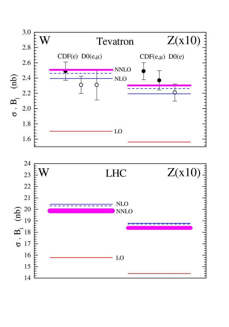
Figure 8: The predictions of the cross sections for $W$ and $Z$ production and leptonic decay at the Tevatron and the LHC obtained from parton sets of the LO, NLO and NNLO global analyses. The cross sections labelled LO, NLO, NLO^′ (dashed line) and NNLO are defined in Eqs. (15,16). The band of NNLO predictions corresponds to the $A,B$ variation of the small–$x$ approximate splitting functions, as discussed in the text. Also shown are measurements obtained at the Tevatron [19, 20]. We take the leptonic branching ratios $B(W\to l\nu)=0.1084$ and $B(Z\to l^{+}l^{-})=0.03364$.

The cross section predictions for $W$ and $Z$ production at the Tevatron and the LHC are shown in Fig. 8, together with data from the CDF [19] and D0 [20] collaborations. The predictions labelled LO, NLO and NNLO are defined (schematically) as follows

$$\sigma_{\scriptstyle\rm LO} = f_{\scriptstyle\rm LO}\otimes f_{\scriptstyle\rm LO}$$

$$\sigma_{\scriptstyle\rm NLO} = f_{\scriptstyle\rm NLO}\otimes f_{\scriptstyle\rm NLO}\otimes\left[\;1\;+\;\alpha_{S,{\scriptstyle\rm NLO}}\;K^{(1)}\;\right]$$

$$\sigma_{\scriptstyle\rm NNLO} = f_{\scriptstyle\rm NNLO}\otimes f_{\scriptstyle\rm NNLO}\otimes\left[\;1\;+\;\alpha_{S,{\scriptstyle\rm NNLO}}\;K^{(1)}\;+\;\left(\alpha_{S,{\scriptstyle\rm NNLO}}\right)^{2}\;K^{(2)}\;\right]$$ (15)

where the label on $\alpha_{S}$ indicates the order to which the $\beta-$function is evaluated. The NLO and NNLO contributions $K^{(1,2)}$ are taken from [21]. The range of NNLO predictions, corresponding to the $A$ or $B$ choice for the approximate NNLO splitting functions, is indicated by the width of the band. As for $F_{L}$, the extrema are given by the $AA$ and $BB$ predictions (see Eq. (2)) with the ‘average’ NNLO partons giving cross sections very close to the centre of the band. Also shown in Fig. 8 (as dashed lines) is the ‘quasi-NLO’ prediction

$$\sigma_{\scriptstyle\rm NLO^{\prime}} = f_{\scriptstyle\rm NLO}\otimes f_{\scriptstyle\rm NLO}\otimes\left[\;1\;+\;\alpha_{S,{\scriptstyle\rm NLO}}\;K^{(1)}\;+\;\left(\alpha_{S,{\scriptstyle\rm NLO}}\right)^{2}\;K^{(2)}\;\right]$$ (16)

which is the expression used in previous MRST estimates of the $W$ and $Z$ cross sections [9, 10]. The NLO^′ predictions enable us to identify the separate NNLO contributions to the cross sections from changing from NLO to NNLO partons and from including the explicit ${\cal O}(\alpha_{S}^{2})$ NNLO coefficient functions ($K^{(2)}$) in the $W,Z$ cross section perturbation series.

The LO $\rightarrow$ NLO $\rightarrow$ NNLO convergence of the predictions is much better than for $F_{L}$, because the boson cross sections depend mainly on the quark distributions at $x\sim 0.05$ (Tevatron) and $x\sim 0.006$ (LHC). Since the global fits include high precision $F_{2}$ data, there is considerable stability in the quark distributions in the sampled $x$ regions, see Fig. 3.

The jump from $\sigma_{\scriptstyle\rm LO}$ to $\sigma_{\scriptstyle\rm NLO}$ is mainly due to the well-known large ${\cal O}(\alpha_{S})$ double logarithmic Drell-Yan K–factor correction arising from soft-gluon emission. The NLO and NNLO cross sections are much closer. By comparing with the NLO^′ predictions, we see that at the Tevatron energy the increase of about $+4\%$ from NLO to NNLO is due in roughly equal parts to the slight increase in the $u$ and $d$ partons in this $x$ range (see Fig. 3), and the net effect of the various $K^{(2)}$ contributions.

At the LHC energy the NLO and NNLO predictions are even closer, because (a) the $K^{(2)}$ contribution is smaller due to an almost complete cancellation between the positive $q\bar{q}$ and negative $qg$ contributions [21], and (b) the quark ratios average to unity at $x\sim 0.006$ for $Q^{2}\sim 10^{4}~{}{\rm GeV}^{2}$, see Fig. 3. The NNLO band is larger than at the Tevatron because the partons are probed at smaller $x$, where there is more uncertainty in the NNLO evolution.

We may conclude from Fig. 8 that perturbative convergence is not a dominant uncertainty in predicting the $W$ and $Z$ cross sections. This stability indicates the potential value of these processes acting as a luminosity monitor for the Tevatron and the LHC.

7 Conclusions

In this paper we have taken a first look at a NNLO global parton analysis of deep inelastic and related hard scattering data. Although the NNLO splitting functions are not fully known, enough information is available to bound their possible behaviour. Even allowing for the full spread of the uncertainties of the functions, we are able to draw interesting conclusions. The inclusion of NNLO effects gives an overall improvement in the description of the data, which is due to the increased scaling violations at both large and small $x$. In a similar manner, if higher-twist contributions are allowed, they decrease in magnitude for both large and small $x$ as we increase the order, approaching very small values for $x\lower 3.01385pt\hbox{$\;\stackrel{{\scriptstyle\textstyle<}}{{\sim}}\;$}0.3$, but remaining large and positive at large $x$. The latter behaviour largely reflects the expectations arising from the presence of heavy target corrections.

Fitting to the data using LO, NLO and NNLO frameworks leads to a hierarchy of gluon distributions at small $x$, such that the NNLO ($\overline{\rm MS}$) input gluon is found to go negative for $x\lower 3.01385pt\hbox{$\;\stackrel{{\scriptstyle\textstyle<}}{{\sim}}\;$}10^{-3}$. However, we stressed that perturbative convergence should be tested for physical observables, rather than for the parton distributions themselves. To this end, the LO, NLO and NNLO predictions were made for the longitudinal structure function $F_{L}$, and for $W$ and $Z$ hadroproduction cross-sections. Although the input gluon goes negative for $x\lower 3.01385pt\hbox{$\;\stackrel{{\scriptstyle\textstyle<}}{{\sim}}\;$}10^{-3}$, we found that $F_{L}$ is positive for $Q^{2}\lower 3.01385pt\hbox{$\;\stackrel{{\scriptstyle\textstyle>}}{{\sim}}\;$}1~{}{\rm GeV}^{2}$. Despite this the form of the predictions for $F_{L}$ show that the DGLAP approach is not convergent until $Q^{2}\sim 5$ GeV². The convergence then improves slowly with increasing $Q^{2}$ and reveals a LO $\rightarrow$ NLO $\rightarrow$ NNLO hierarchy in the predictions for $F_{L}$, which mirrors that of the gluon but with increased stability. A measure of the uncertainty is the $\sim 15\%$ change in $F_{L}$ in going from the NLO to NNLO prediction at $x\sim 10^{-3}$ and $Q^{2}\sim 100~{}{\rm GeV}^{2}$. The convergence deteriorates with decreasing $x$ and most likely is due to the neglect of $\log(1/x)$ contributions beyond the NNLO DGLAP framework. At low $Q^{2}$ ($Q^{2}\lower 3.01385pt\hbox{$\;\stackrel{{\scriptstyle\textstyle<}}{{\sim}}\;$}5~{}{\rm GeV}^{2}$) the $\log(1/x)$ terms are even more important. There is also the possibility of higher-twist contributions, which for $F_{L}$ may be different at small $x$ from those for $F_{2}$ [27]. On the other hand the predictions of the $W$ and $Z$ hadroproduction cross sections are rather stable, due to the more direct relation between the fitted data and the predictions.

Here we have addressed, in an exploratory fashion, theoretical issues arising from including NNLO corrections in global parton analyses of deep inelastic and related data. However new HERA data with increased precision will soon be available. These will be included in a new global analysis to yield both an updated set of NLO partons and a first set of NNLO distributions.

Appendix : NNLO treatment of heavy flavour partons

For the treatment of heavy flavours we use an approximate NNLO generalization of the Thorne-Roberts variable flavour number scheme (VFNS). This scheme was presented in detail in [22], and the general framework outlined for all orders in perturbation theory. Essentially one obtains the VFNS coefficient functions in terms of the fixed flavour number scheme (FFNS) coefficient functions and partonic matrix elements $A_{ab}$. The former are the coefficient functions calculated assuming that the heavy quark (denoted by $H$) has no parton distribution, but may only be created via a hard scattering process. The matrix elements define the $(n_{f}+1)$–flavour parton distributions in terms of the $n_{f}$–flavour parton distributions, i.e. the $A_{Ha}$ tell one how the heavy quark distribution is constructed from the light partons and the $A_{ab,H}$ tell one how the light parton distributions are altered by internal heavy quarks (in particular $A_{ab,H}^{(0)}=\delta_{ab}$). The VFNS coefficient functions are determined by solving Eqs. (3.5)-(3.9) in the latter of [22]. For example,

$$C^{{\rm FF}(n)}_{Hg}=\sum_{m=0}^{n}C^{{\rm VF}(n-m)}_{Hg}\otimes A^{(m)}_{gg,H}+n_{f}C^{{\rm VF,PS}(n-m)}_{Hq}\otimes A^{(m)}_{qg,H}+[C^{{\rm VF,NS}(n-m)}_{HH}+C^{{\rm VF,PS}(n-m)}_{HH}]\otimes A^{(m)}_{Hg}.$$ (17)

The matrix elements and FFNS coefficient functions are unambiguously calculable, but there is some element of choice in the VFNS coefficient functions since there are more degrees of freedom than there are constraining equations. One may eliminate this ambiguity by simply calculating diagrams assuming one has initial state heavy partons and keeping mass dependent terms. However, this leads to unphysical threshold behaviour for the coefficient functions, and we choose instead to impose as physical a constraint as possible. Hence, we make the derivative of $F_{2}^{H}(x,Q^{2})$ continuous in the gluon sector (which overwhelmingly dominates) as one switches from FFNS to VFNS coefficient functions and turns on the heavy quark parton distribution at $Q^{2}=m_{H}^{2}$. This choice of VFNS coefficient functions is essentially a freedom in factorization schemes, with all schemes becoming identical when summed to all orders, but differing by terms $\sim m_{H}^{2}/Q^{2}$ at finite order.

At NNLO, all VFNSs experience two related technical complications due to internal quark loops which may or may not be cut. First, it has long been known that the parton distributions become discontinuous at $\mu^{2}=m_{H}^{2}$ at ${\cal O}(\alpha_{S}^{2})$ [23]. For example, the heavy quark distribution at $\mu^{2}=m_{H}^{2}$ becomes

$$(H+\bar{H})^{(2)}\>(x,m_{H}^{2})=\biggl{(}\frac{\alpha_{S}(m_{H}^{2})}{2\pi}\biggr{)}^{2}[A^{(2)}_{Hg}\otimes g(m_{H}^{2})+A^{(2)}_{Hq}\otimes q(m_{H}^{2})].$$ (18)

The gluon and light quarks also acquire discontinuities as the heavy parton distribution is turned on, such that momentum is conserved, see [23]. These lead to a corresponding discontinuity in the coefficient functions, maintaining the continuity of the structure functions, e.g. solving (17) at NNLO at $\mu^{2}=m_{H}^{2}$ one obtains

$$C^{{\rm FF}(2)}_{Hg}=C^{{\rm VF}(2)}_{Hg}+C^{{\rm VF,NS}(0)}_{HH}\otimes A^{(2)}_{Hg}.$$ (19)

The second complication at NNLO arises because the heavy quarks in the final states are no longer just those coupling directly to the external vector boson probe, but can be generated even when it is a light quark coupling to this probe. In principle it is a technical shortcoming of our scheme that the implicit definition of the heavy quark structure function involves the heavy quark coupling to the external vector boson. This simplifies the factorization, but is not strictly physically correct. A more general prescription is discussed in [24], where a cut in invariant mass has to be implemented above which heavy quark-antiquark pairs generated away from the external vertex may be defined as observable.

In this paper we simply ignore both these complications. This is due to the fact that the whole analysis is approximate and also because both lead to effects which in practice are extremely small – especially when compared to other uncertainties. Both complications should be dealt with in a truly precise NNLO analysis once the exact NNLO splitting functions are known, though we are confident that they (especially the latter) will lead to tiny effects. However, at present we do not even know the NNLO, i.e. ${\cal O}(\alpha_{S}^{3})$, FFNS coefficient functions, so a precise VFNS is impossible to define.

Nevertheless, this is where our heavy flavour prescription comes into its own. Other prescriptions [26, 24] which use the coefficient functions from diagrams involving single initial state heavy partons rely on precise cancellations between the heavy quark distributions and terms involving the VFNS coefficient functions in order to maintain smooth behaviour. For example, at NNLO a large contribution to the heavy quark evolution from $\alpha_{S}^{3}P^{(2)}_{qg}$ needs to be cancelled by a term $\alpha_{S}^{3}P^{(2)}_{qg}\ln(\mu^{2}/m_{H}^{2})C^{{\rm VF}(0)}_{2,HH}\otimes g(\mu^{2})$ to avoid too quick a growth of $F_{2}^{H}(x,Q^{2})$ for $\mu^{2}$ just above $m_{c}^{2}$. In our prescription the correct threshold behaviour is built into $C^{{\rm VF}(0)}_{2,HH}$ automatically, i.e. $C^{{\rm VF}(0)}_{2,HH}=0$ if $W^{2}<4m_{H}^{2}$, and such precise cancellations are not necessary – simply including NNLO evolution of the heavy quarks without NNLO heavy quark coefficient functions at all maintains smooth behaviour. However, we want to obtain the correct NNLO high $Q^{2}$ limit. Hence, we include the massless ${\cal O}(\alpha_{S}^{2})$ coefficient functions for the heavy quarks, but weighted by a factor of $\beta=(1-4m_{H}^{2}z/(Q^{2}(1-z))^{0.5}$, i.e. the velocity of the heavy quark in the centre of mass system, to impose the correct threshold behaviour at low $Q^{2}$. This procedure is very simplistic, but it contains all the relevant physics. Significant improvements to this approximate procedure would require the NNLO FFNS coefficient functions.

Finally, we note that the heavy flavour longitudinal coefficient functions behave like $\beta^{3}$, and thus are heavily suppressed until very high $Q^{2}$. At such high $Q^{2}$, the ${\cal O}(\alpha_{S}^{3})$ coefficient functions have become relatively unimportant, and hence we simply omit the ${\cal O}(\alpha_{S}^{3})$ longitudinal coefficient functions until a more precise analysis is possible.

Figure 1: The description of data [12] for the $F_{2}$ structure function at a few representative $x$ values obtained in the LO, NLO and NNLO global parton analyses.

Figure 2: The description of data [12] for the $F_{2}$ structure function at large $x$ obtained in the LO, NLO and NNLO global parton analyses.

Figure 3: A comparison of partons obtained in the ‘central’ NNLO analysis with those obtained in the NLO fit, first at $Q^{2}=10$ GeV² and then at $Q^{2}=10^{4}$ GeV². We show the NNLO/NLO ratios for the gluon and the up and down quark distributions.

Figure 4: The evolution of the gluon obtained in the LO, NLO and NNLO global analyses. The gluons obtained using the extreme forms, $A$ and $B$, of the NNLO splitting functions are shown (dot-dashed curves), together with that from the average (continuous curves).

Figure 5: The behaviour of the NNLO contributions to the coefficient function $xC^{(3)}_{L,g}(x)$ for $F_{L}$ taking $n_{f}=3$. The average of the two extreme behaviours is shown.

Figure 6: The predictions for the longitudinal structure function $F_{L}$ obtained from the LO, NLO and NNLO sets of partons. The NNLO extremes (using parton uncertainty alone) are plotted only for $Q^{2}=2$ GeV².

Figure 7: The NLO/LO and NNLO/NLO ratios of the predictions of $F_{L}$, at two different values of $Q^{2}$, shown to indicate the degree of perturbative stability of the analysis.

References

-
[1]
H1 Collaboration: C. Adloff et al., Eur. Phys. J.
C13 (2000) 609;
M Klein, Rapporteur’s talk, Lepton Photon Symposium 1999, SLAC hep-ex/0001059 includes a review of preliminary HERA data;
N. Tuning, talk at 8th International Workshop on Deep-Inelastic Scattering and QCD, Liverpool, (April 2000). -
[2]
E.B. Zijlstra and W.L. van Neerven, Phys. Lett. B272 (1991)
127; ibid B273 (1991) 476; ibid B297 (1992) 377;
E.B. Zijlstra and W.L. van Neerven, Nucl. Phys. B383 (1992) 525. - [3] S.A. Larin, P. Nogueira, T. van Ritbergen and J.A.M. Vermaseren, Nucl. Phys. B492 (1997) 338.
-
[4]
S. Catani and F. Hautmann, Nucl. Phys. B427 (1994) 475;
V.S. Fadin and L.N. Lipatov, Phys. Lett. B429 (1998) 127;
G. Camici and M. Ciafaloni, Phys. Lett. B430 (1998) 349. - [5] J. Blümlein and A. Vogt, Phys. Lett. B370 (1996) 149.
- [6] J.A. Gracey, Phys. Lett. B322 (1994) 141.
- [7] J.F. Bennett and J.A. Gracey, Nucl. Phys. B517 (1998) 241.
-
[8]
W.L. van Neerven and A. Vogt, Nucl. Phys. B568
(2000) 263;
W.L. van Neerven and A. Vogt, in the QCD section of the Proc. of the LHC CERN Workshop, hep-ph/0005025;
W.L. van Neerven and A. Vogt, hep-ph/0006154. - [9] A.D. Martin, R.G. Roberts, W.J. Stirling and R.S. Thorne, Eur. Phys. J. C4 (1998) 463.
- [10] A.D. Martin, R.G. Roberts, W.J. Stirling and R.S. Thorne, Eur. Phys. J. C14 (2000) 133.
-
[11]
J. Huston et al., Phys. Rev. D51 (1995) 6139;
P. Aurenche, M. Fontannaz, J.Ph. Guillet, B. Kniehl, E. Pilon, M. Werlen, Eur. Phys. J. C9 (1999) 107;
L. Apanasevich et al., Phys. Rev. D59 (1999) 074007;
S. Catani, M. Mangano, P. Nason, C. Oleari and W. Vogelsang, JHEP 9903:025 (1999);
H-L. Lai and H-N. Li, Phys. Rev. D58 (1998) 114020;
M.A. Kimber, A.D. Martin and M.G. Ryskin, Eur. Phys. J. C12 (2000) 665;
E. Laenen, G. Sterman and W. Vogelsang, Phys. Rev. Lett. 84 (2000) 4296. -
[12]
ZEUS collaboration: M. Derrick et al., Zeit. Phys. C69
(1996) 607 ; M. Derrick et al., Zeit. Phys. C72 (1996) 399;
H1 collaboration: S. Aid et al., Nucl. Phys. B470 (1996) 3; C. Adloff et al., Nucl. Phys. B497 (1997) 3; C. Adloff et al. Eur. Phys. J. C13 (2000) 609;
NMCollaboration: M. Arneodo et al., Nucl. Phys. B483 (1997) 3;
E665 collaboration: M.R. Adams et al., Phys. Rev. D54 (1996) 3006;
BCDMS collaboration: A.C. Benvenuti et al., Phys. Lett. B223 (1989) 485;
L.W. Whitlow et al., Phys. Lett. B282 (1992) 475. - [13] A.D. Martin, R.G. Roberts, W.J. Stirling and R.S. Thorne, Phys. Lett. B443 (1998) 301.
-
[14]
A.L. Kataev, A.V. Kotikov, G. Parente and A.V. Sidorov, Phys.
Lett. B417 (1998) 374;
A.L. Kataev, G. Parente, A.V. Sidorov, Nucl. Phys. B563 (2000) 405. - [15] U.K. Yang and A. Bodek, Eur. Phys. J. C13 (2000) 241.
- [16] E. Stein, M. Meyer-Hermann, L. Mankiewicz and A. Schäfer, Phys. Lett. B376 (1996) 177.
- [17] J. Sánchez Guillén et al., Nucl. Phys. B353 (1990) 337.
- [18] R. Akhoury, M.G. Sotiropoulos and G. Sterman, Phys. Rev. Lett. 81 (1998) 3819.
- [19] CDF collaboration: T. Affolder et al., Phys. Rev. Lett. 84 (2000) 845; F. Abe et al., Phys. Rev. D59 (1999) 052002; F. Abe et al., Phys. Rev. Lett. 76 (1996) 3070.
- [20] D0 collaboration: B. Abbott et al., Phys. Rev. D60 (1999) 052003; J. Ellison, presentation at the EPS-HEP99 Conference, Tampere, Finland, July 1999.
-
[21]
R. Hamburg, T. Matsuura and W.L. van Neerven, Nucl. Phys.
B345 (1990) 331; Nucl. Phys. B359 (1991) 343;
W.L. van Neerven and E.B. Zijlstra, Nucl. Phys. B382 (1992) 11. - [22] R.S. Thorne and R.G. Roberts, Phys. Lett. B421 (1998) 303; Phys. Rev. D57 (1998) 6871.
-
[23]
M. Buza et al., Nucl. Phys. B472 (1996) 611;
M. Buza et al., Eur. Phys. J. C1 (1998) 301. - [24] A. Chuvakin, J. Smith and W.L. van Neerven, Phys. Rev. D61 (2000) 096004.
- [25] M. Glück, E. Reya and A. Vogt, Eur. Phys. J. C5 (1998) 461.
- [26] M. Aivazis, J.C. Collins, F. Olness and W.K. Tung, Phys. Rev. D50 (1994) 3102.
- [27] J. Bartels and C. Bontus, Phys. Rev. D61 (2000) 034009.